Realistic Noise Synthesis with Diffusion Models

Abstract

Deep image denoising models often rely on large amount of training data for the high quality performance. However, it is challenging to obtain sufficient amount of data under real-world scenarios for the supervised training. As such, synthesizing realistic noise becomes an important solution. However, existing techniques have limitations in modeling complex noise distributions, resulting in residual noise and edge artifacts in denoising methods relying on synthetic data. To overcome these challenges, we propose a novel method that synthesizes realistic noise using diffusion models, namely Realistic Noise Synthesize Diffusor (RNSD). In particular, the proposed time-aware controlling module can simulate various environmental conditions under given camera settings. RNSD can incorporate guided multiscale content, such that more realistic noise with spatial correlations can be generated at multiple frequencies. In addition, we construct an inversion mechanism to predict the unknown camera setting, which enables the extension of RNSD to datasets without setting information. Extensive experiments demonstrate that our RNSD method significantly outperforms the existing methods not only in the synthesized noise under multiple realism metrics, but also in the single image denoising performances.

Introduction

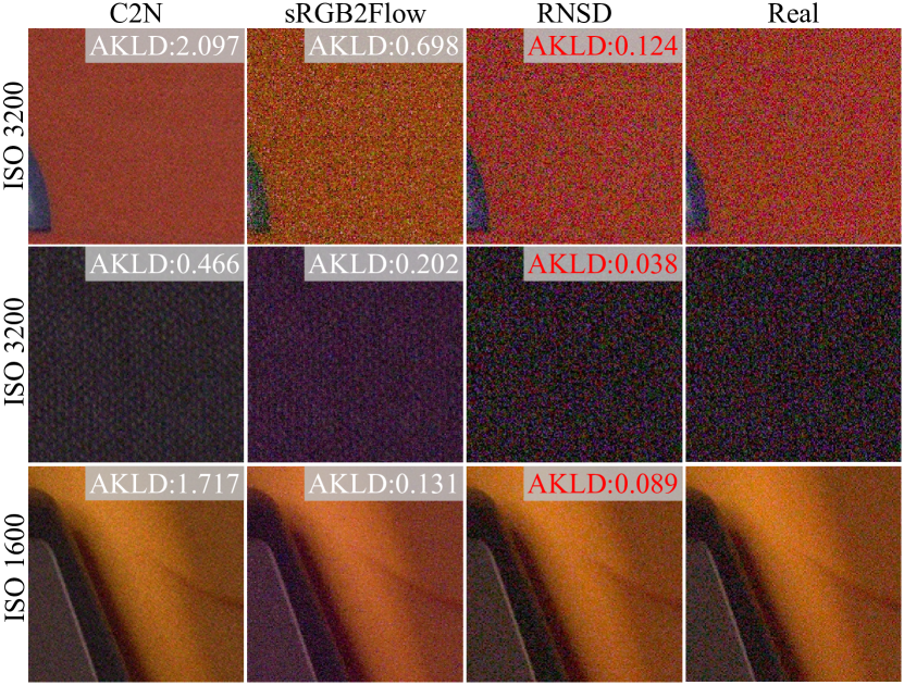
Figure 1: Visual results and similarity metric AKLD (Yue et al. 2020) of noise synthesis using different methods, including C2N (Jang et al. 2021), sRGB2Flow (Kousha et al. 2022), and our RNSD results. Images are from the SIDD dataset (Abdelhamed, Lin, and Brown 2018) and our method achieves the best results, compared to other state-of-the-art methods, at different ISOs.

Due to factors such as sensors, image signal processor (ISP), image compression, and environment, image noise often exhibits complex spatial correlation. Therefore, in deep learning, as an ill-posed problem, image denoising (Wang et al. 2022; Zamir et al. 2021, 2022; Guo et al. 2019; Zhang, Zuo, and Zhang 2018; Kim et al. 2020) often requires supervised training with a large amount of data pairs. For a clean image $\mathbf{s}$, its noisy version can be simply represented as $\mathbf{y}$, where $\mathbf{n}$ represents the noise.

$$\mathbf{y}=\mathbf{s}+\mathbf{n}.$$ (1)

Under the assumption of independent $\mathbf{s}$ and $\mathbf{n}$, the collection method of most datasets (Abdelhamed, Lin, and Brown 2018; Plotz and Roth 2017; Xu et al. 2018; Nam et al. 2016) is based on the assumption that $E(\mathbf{n})=0$ (i.e., noise expectation is zero), resulting in obtaining a reference image (ground truth) by averaging multiple frames of the same static scene. However, subsequent complex ISP nonlinear operations like demosaicing, local tone mapping, and sharpening can induce complex spatial correlations in noise. This causes real noise to deviate from the assumption of spatial independence, making it difficult to obtain a true noise-free reference image through multi-frame averaging. Furthermore, the requirement for multiple static frames over a short time period restricts the variety of scenes that can be captured. As a result, collecting real noise data with diverse content is an extremely difficult and labor-intensive task.

Some methods (Foi et al. 2008; Foi 2009; Brooks et al. 2019) attempt to model $\mathbf{n}$ using Gaussian white noise ignoring the spatial correlation of realistic noise. Furthermore, motivated by the generative power of GANs, a large number of GAN-based generation methods attempt to model real noise in the latent space. Nevertheless, GANs are highly unstable during training due to the lack of a strict likelihood function, and are prone to mode collapse when dealing with complex and varied noise distributions. As a result, there is often a large gap between the distribution of generated noise and the real noise distribution. In contrast, the diffusion model (Ho, Jain, and Abbeel 2020; Song, Meng, and Ermon 2020; San-Roman, Nachmani, and Wolf 2021; Bansal et al. 2022; Chen et al. 2022b) with a rigorous likelihood derivation can sample the target image from a pure Gaussian distribution and has more varied and stable image generation capabilities. However, there is currently no successful solution applying diffusion to the field of synthetic noise due to the confusion between the tasks of diffusion-based denoising and synthetic noise generation, as well as the lack of condition design for multi-modal noise.

In this paper, we introduce RNSD, a novel method for synthesizing realistic noise data based on the diffusion model. RNSD has the capability to generate a large amount of noise images that closely resemble the distribution of real-world noise by leveraging high-quality, low-noise samples. The augmented data significantly enhances the performance of denoising models, both in terms of noise reduction and resolution.

Specifically, RNSD use real noisy images $\mathbf{y}$ as initial state $\mathbf{x_{0}}$ to build Generated Noise Diffusion. Time-aware camera setting (cs) condition module CamSampler is designed to accommodate multi-modal noise distributions, which utilizes camera setting information to control the diffusion-generated results. Additionally, we employ multi-scale content conditioning MCG-UNet to guide the generation of signal-correlated noise by identifying shared characteristics across different noise levels and distributions. Finally, we propose a CamPredictor module to predict camera setting information from clean images and this mechanism leverages a trained diffusion network as a penalty term to minimize the discrepancies in generated noise distributions across various datasets.

To summarize, our main contributions are as follows:

• We first propose a real noise data synthesis approach RNSD based on the diffusion model.

• We design a camera setting embedding module CamSamper that can better control the distribution and level of generated noise. Specially, a inversion mechanism CamPredictor is designed to predict the camera settings, enabling diffusion to generate noise distributions that better match the real noise distribution on a wide range of datasets without camera settings.

• By constructing a network with multi-scale content guidance MCG-UNet, we can enable the diffusion process to progressively learn noise distribution from spatially independent to spatially dependent, reducing the gap between noise distributions.

• Our approach achieves state-of-the-art results on multiple benchmarks and metrics, significantly enhancing the performance of denoising models with improvements of up to 0.6dB in PSNR on NAFNet (Chen et al. 2022a).

Related Work

Noise Model.

From the perspective of digital imaging, the main sources of noise are read noise, shot noise, and fixed-pattern noise. Some methods (Foi et al. 2008; Foi 2009) model it as a classical Gaussian-Poisson model, read noise is signal-independent and can be modeled as Gaussian noise, while shot noise is signal-dependent and can be modeled as Poisson noise. Among them, shot noise is approximated as Gaussian noise and has been widely used (Brooks et al. 2019; Guo et al. 2019). Despite that, subsequent complex ISP nonlinear operations such as demosaicing, local tone mapping(LTM), high dynamic range(HDR), sharpening, denoising, etc., can cause the noise distribution to lose its regularity and the noise shape to exhibit more complex spatial correlations, making it difficult for traditional methods to model real noise.

Simulation-based ISP methods.

To address the impact of ISP on the distribution and shape of real noise, some methods have begun to synthesize more realistic noise by studying ISP simulations. Guo $et.al$ (Guo et al. 2019) employed traditional methods to simulate the ISP operations of RGB to Bayer and Bayer to RGB. Zamir $et.al$ (Zamir et al. 2020) builds a complete network for RGB2RAW and RAW2RGB using deep learning to simulate the ISP operations of different sensors and obtain a model for synthesizing real noise data through learning. Considering the loss caused by the differences between forward and inverse ISP processing, Xing $et.al$ (Xing, Qian, and Chen 2021) builds a reversible ISP network to simulate this process. Abdelhamed $et.al$ (Abdelhamed, Brubaker, and Brown 2019) simulated this process from the perspective of learning normalizing flow by sampling noise from the Gaussian distribution through inverse mapping, and Kousha $et.al$ (Kousha et al. 2022) further improved the results and applied it to the sRGB domain. However, existing methods have not fully addressed the limitations of simulating ISP. Simulating ISP remains challenging due to its intricate and sensor-specific nature. Moreover, ISP simulation requires substantial data which is difficult to generate.

GAN-based methods.

In recent years, the powerful data distribution fitting ability of GANs  (Karras et al. 2017; Karras, Laine, and Aila 2019; Brock, Donahue, and Simonyan 2018; Shaham, Dekel, and Michaeli 2019) in image generation has attracted extensive research. Real noise itself can also be seen as a type of data distribution, so there are many works on synthesizing real noise based on GANs. By using Gaussian noise as input to control randomness and separating independent and correlated noise, Jiang $et.al$ (Jang et al. 2021)showed that GANs can be used to synthesize real noise under unsupervised conditions with unpaired data. Cai $et.al$ (Cai et al. 2021) introduced a pre-training network to separately align the generated content domain and noise domain. Although GANs have made considerable progress in synthesizing noise, the lack of a tractable likelihood makes it difficult to assess the quality of the synthesized images.

Diffusion methods.

Real noise has a complex and diverse distribution that is influenced by many factors such as sensor, iso, and isp. As a result, GANs may suffer from mode collapse when synthesizing real noise. In contrast, diffusion-based methods(Ho, Jain, and Abbeel 2020; Song, Meng, and Ermon 2020; San-Roman, Nachmani, and Wolf 2021; Bansal et al. 2022; Chen et al. 2022b) do not have this problem and can generate more diverse results, providing a more complete modeling of the data distribution. Additionally, by adjusting the diffusion steps and noise levels, diffusion-based methods can generate samples with specific properties and characteristics, enabling more precise and controllable synthesis of real noise data. Nevertheless, diffusion model has not been successfully applied to synthetic noise generation, partly due to the confusion with diffusion-based denoising and the lack of conditional models for complex noise distributions. With our proposed RNSD method, we address these limitations.

Methodology

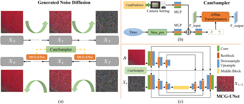
Figure 2: (a) Generated noise diffusion’s pipeline of RNSD. (b) The pipeline of our CamSampler and CamPredictor (c) The architecture of the MCG-UNet model we designed.

Generated Noise Diffusion

Traditional diffusion models are usually trained on noise-free style data, which can sample target domain images from any Gaussian noise distribution. In contrast, we treat images with real noise distributions as target domain images in order to sample real noise distributions from any Gaussian noise distribution. By replacing $\mathbf{x}_{0}$ with real noise distribution data $\mathbf{y}$ and through simple settings, the diffusion model can generate data that satisfies the real noise distribution.

Specifically, we adopt the probability model of DDPM (Ho, Jain, and Abbeel 2020). During the forward process, a Markov chain structure to maximize the posterior $q(\mathbf{x}_{T}|\mathbf{x}_{0})$ and sample $\mathbf{x}_{0}$ to a pure Gaussian distribution $\mathbf{x}_{T}$ with a variance noise intensity $\beta_{t}$:

$$q(\mathbf{x}_{T}|\mathbf{x}_{0})=\prod\limits_{t=1}^{T}q(\mathbf{x}_{t}|\mathbf{x}_{t-1}),$$ (2)

$$q(\mathbf{x}_{t}|\mathbf{x}_{t-1})=\mathcal{N}(\mathbf{x}_{t};\sqrt{1-\beta_{t}}\mathbf{x}_{t-1},\beta_{t}\mathbf{I}),$$

where $\mathbf{I}$ is a unit covariance matrix and $T$ is the total number of sampling steps. The general sampling process is obtained by inversely solving a Gaussian Markov chain process, which can be understood as gradual denoising from the above Gaussian distribution $\mathbf{x}_{T}$ to obtain the sampled result $\mathbf{x}_{0}$:

$$p_{\theta}(\mathbf{x}_{0:T})=p(\mathbf{x}_{T})\prod\limits_{t=1}^{T}p_{\theta}(\mathbf{x}_{t-1}|\mathbf{x}_{t}),$$ (3)

$$p_{\theta}(\mathbf{x}_{t-1}|\mathbf{x}_{t})=\mathcal{N}(\mathbf{x}_{t-1};\mu_{\theta}(\mathbf{x}_{t},t),\mathbf{\sum}_{\theta}(\mathbf{x}_{t},t)),$$

where $\mu_{\theta}$ and $\sum_{\theta}$ are the parameters of the conditional noise distribution estimated by the network for the current sample. To address the characteristics of real noise distribution and morphological heterogeneity, we introduce a more targeted conditioning mechanism using MCG-UNet and the CamSampler module, making the posterior probability controllable, mathematically, the process is:

$$p_{\theta}(\mathbf{x}_{t-1}|\mathbf{x}_{t})=\mathcal{N}(\mathbf{x}_{t-1};\mathbf{\mu},\mathbf{\sigma}),$$ (4)

$$\mathbf{\mu}=\mathbf{\mu}_{\theta}(\mathbf{x}_{t},\mathbf{s},cs,t),$$

$$\mathbf{\sigma}=\mathbf{\sum}_{\theta}(\mathbf{x}_{t},\mathbf{s},cs,t),$$

based on this, with the idea of deterministic sampling using DDIM (Song, Meng, and Ermon 2020), our overall algorithmic flow is illustrated in Algorithm. 1, $\mathbf{s}$ and $cs$ are additional information we introduce, representing clean images and camera settings, respectively. Both $\mathbf{s}$ and $cs$ are used as conditioning information to control the content of the generated image, mainly regulating its spatial variation and related noise distributions.

Algorithm 1 Control Sampling

1:  $\mathbf{x}_{T}\sim{\mathcal{N}(0,1)}$

2:  for $t=T,...,1$ do

3:     $\alpha_{t}=1-\beta_{t}$, $\overline{\alpha}_{t}=\prod_{s=1}^{t}\alpha_{s}$

4:     $\beta,\gamma=$CamSampler$(t,cs)$

5:     $\mathbf{\epsilon}_{\theta}=$MCG-UNet$(\mathbf{x}_{t},\mathbf{s},\beta,\gamma)$

6:     $\mathbf{x}_{t-1}=\sqrt{\overline{\alpha}_{t-1}}(\frac{\mathbf{x}_{t}-\sqrt{1-\overline{\alpha}_{t}}\mathbf{\epsilon}_{\theta}}{\sqrt{\overline{\alpha}_{t}}})+\sqrt{1-\overline{\alpha}_{t-1}}\mathbf{\epsilon}_{\theta}$

7:  end for

8:  $\mathbf{y}=\mathbf{x}_{0}$

9:  return  $\mathbf{y}$

CamSampler: Time-aware Dynamic Setting Mechanism

Real noise distributions are usually determined by multiple factors, including ISO gain, exposure time, color temperature, brightness, and other factors. As shown in Eq. 5:

$$\mathbf{\triangledown}_{\theta}||\mathbf{\epsilon}_{t}-\mathbf{\epsilon}_{\theta}(\mathbf{x}_{t},t)||,$$ (5)

where normal diffusion only learns the noise distribution across different samplings through $t$. Without distinguishing noise distribution under different conditions, it is difficult for traditional methods to learn a generalized distribution from complex noise based on spatial photometric variations, iso changes, and sensor variations.

The most fundamental reason is that the noise distribution under different conditions varies significantly, for example, the noise across different sensors can exhibit completely different distributions. During the learning process, the network tends to converge the target to the overall expectation of the data set, leading to fixed-mode noise patterns and distributions that cause differences between the generated and target noise. In contrast, just as the Eq. 6:

$$\mathbf{\triangledown}_{\theta}||\epsilon_{t}-\epsilon_{\theta}(\mathbf{x}_{t},t,cs)||,$$ (6)

$$cs=\mathbf{\phi}(iso,et,st,ct,bm),$$

we introduce five factors, including ISO ($iso$), exposure time ($et$), sensor type ($st$), color temperature ($ct$), and brightness mode ($bm$), as conditions to control the generation of noise. By introducing such explicit priors, we can narrow down the learning domain of the network and enable it to approximate more complex and variable noise distributions.

In particular, a simple concatenation of camera settings cannot fully achieve the intended effect. Generally speaking, we believe that the influence of camera settings should vary with sampling steps. For example, sensor information strongly correlated with ISP determines the basic form of noise, and its impact on noise is usually coupled with high-frequency information in image content. That is, when $t$ tends to $T$, the weight of camera settings’ influence is greater than when $t$ tends to 0. To address this issue, we propose a CamSampler with a dynamic setting mechanism, that the weights influences of different factors will vary with sampling steps. Specifically, as shown in Fig. 2 (b), the process is:

$$\mathbf{embeds}=MLP_{1}(pos\_emb(t))+MLP_{2}(cs),$$ (7)

$$\beta,\gamma=MLP_{3}(\mathbf{embeds}).$$

we use a Multilayer Perceptron (MLP) to encode the camera settings together with the sampling steps to parameters ${\beta}$ and ${\gamma}$ at each layer of UNet, which is capable of dynamic setting influence mechanism through applying affine transformations to each layer of features in UNet.

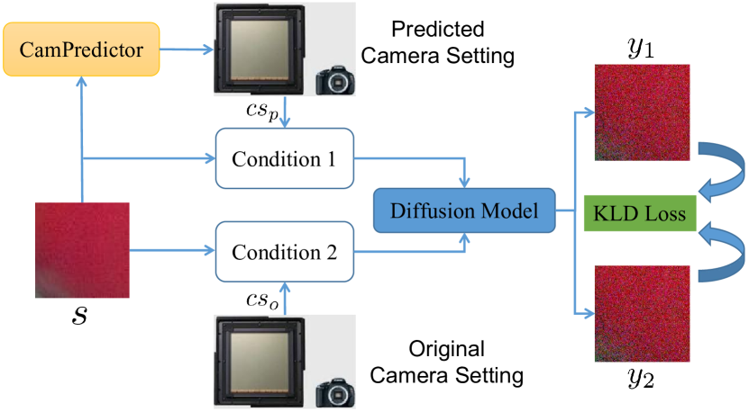
Figure 3: Training pipeline of CamPredictor.

Multi-scale Content Guided Dual UNet (MCG-UNet)

The distribution of real noise is usually strongly correlated with brightness. This is generally due to the different photon information received in different brightness regions, as well as the heterogeneity caused by ISP post-processing. Clean images can to some extent reflect the total amount of photons received in different regions, so they can be used as the main guidance information for generating noise in diffusion.

Zhou $et.al$ (Zhou et al. 2020) proposed that after downsampling, spatially varying and spatially correlated noise will become spatially varying but spatially uncorrelated noise. In other words, for real noise, which spans multiple frequency ranges, noise at different frequencies is coupled with image information at different frequencies.

In particular, we introduce a Multi-scale Content Guided Dual UNet (MCG-UNet), as shown in Fig. 2 (c), which can simulate the coupling relationship between noise and image information at different frequencies. Mathematically, the process is:

$$\mathbf{F}_{\mathbf{x}_{t_{i}}}=encoder_{i}(\mathbf{x}_{t}),$$ (8)

$$\mathbf{F}_{\mathbf{s}_{i}}=encoder_{i}(\mathbf{s}),i=1,2,3,$$

$$\mathbf{F}_{\mathbf{o}_{i}}=decoder_{i}(Concat(\mathbf{F}_{i},\mathbf{F}_{\mathbf{s}_{i}},\mathbf{F}_{\mathbf{x}_{t_{i}}})),$$

we use symmetric but non-shared weight networks to extract features of both $\mathbf{x}_{t}$ and clean image $\mathbf{s}$ at the three downsampling stages of the encoder. In addition to the normal skip connections in the decoder stage of UNet, we also add multi-scale feature of clean image $\mathbf{F}_{\mathbf{s}_{i}}$ in the three upsampling stages.

CamPredictor: Setting Inversion Mechanism

When we only have arbitrary clean images without camera setting information, in order to utilize our noise synthesis method, we design a CNN-based CamPredictor model as an assistance. This module takes clean images as input and predicts their corresponding camera settings because we believe there exists a significant correlation between camera settings and the final captured image information. Specifically, we use ResNet50 (He et al. 2016) as the backbone architecture for the CamPredictor model.

Figure 4: Noisy synthesis samples from different methods, including C2N, sRGB2Flow, and RNSD. Codes on the left indicate [camera]-[ISO]-[brightness].

As shown in Fig. 3, during training, we first input a clean image $\mathbf{s}$ into CamPredictor to obtain its corresponding camera setting vector $cs_{p}$. We then use this clean image $\mathbf{s}$ and predicted vector $cs_{p}$ as the condition inputs for the diffusion model to get the noisy image $\mathbf{y}_{1}$, with the parameters of the MCG-UNet module frozen, and the sampling step $t$ is randomly generated. We also input the same clean image $\mathbf{s}$ and its corresponding original camera setting vector $cs_{o}$ to the diffusion model to obtain a noisy image $\mathbf{y}_{2}$ as the ground truth (with consistent $t$). We calculate the KLD metric between the two output noisy images as the loss to train the CamPredictor network. Mathematically, the process is

$$cs_{p}=CamPredictor(\mathbf{s}),$$ (9)

$$\mathbf{y}_{1}=\epsilon_{\theta}(\mathbf{x}_{t},t,cs_{p},\mathbf{s}),$$

$$\mathbf{y}_{2}=\epsilon_{\theta}(\mathbf{x}_{t},t,cs_{o},\mathbf{s}),$$

$$\mathcal{L}=KLD(\mathbf{y}_{1},\mathbf{y}_{2}).$$

During the noise synthesis stage, we leverage the trained CamPredictor model to predict the camera settings for any given image, enabling us to generate noise that better matches the scene-specific characteristics of the input image.

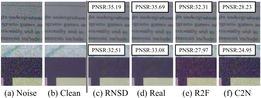
Figure 5: Denoising results on SIDD Validation from DnCNN trained on noisy images from (d) real noisy images of SIDD Meduim, (c) RNSD, and (e, f) two of other baselines

Experiments

Experimental Settings

Datasets.

In the experimental setup, we use the SIDD small dataset (Abdelhamed, Lin, and Brown 2018) for both the diffusion model training of noise generation and as part of the denoising experiments. This dataset contains 160 image pairs of noisy and clean smartphone photos captured by 5 different cameras. For validating both the noise generation and image denoising tasks, we use the SIDD Validation dataset, which contains 40 pairs of noisy and clean images from the same 5 smartphone cameras. We also utilize the SIDD Medium dataset, containing 320 image pairs, to evaluate the effectiveness of our synthesized noise for the denoising task. In addition, we select part of images from the LSDIR dataset (Li et al. 2023) containing 84,991 high-quality training samples to augment the data for training various denoising models.

Evaluation and Metrics.

To evaluate noise generation, we use two metrics from  (Yue et al. 2020): PSNR Gap (PGap) and Average KL Divergence (AKLD). PGap indirectly compares synthesized and real noisy images via the performance of a trained denoising model, with a smaller PGap indicating better noise generation. AKLD measures the similarity between the distributions of real and synthetic noisy images, with lower values indicating better performance. We also use Peak Signal-to-Noise Ratio (PSNR) and Structural Similarity Index (SSIM) to evaluate the performance of different denoising models.

	SIDD Validation
Method	DnCNN-B		RIDNet		NAFNet
Metric	PSNR$\uparrow$	SSIM$\uparrow$	PSNR$\uparrow$	SSIM$\uparrow$	PSNR$\uparrow$	SSIM$\uparrow$
SIDD small	37.70	0.941	38.30	0.947	38.95	0.954
SIDD small+sRGB2flow	37.53	0.936	38.28	0.946	39.00	0.954
SIDD small+RNSD	38.27	0.946	38.84	0.952	39.56	0.958
SIDD medium	38.34	0.947	38.77	0.952	40.30	0.962
SIDD medium+RNSD*	38.64	0.950	39.08	0.954	40.36	0.962

Table 1: The synthetic data model trained on the small dataset exhibits improvement in denoising performance for several baseline models such as DnCNN-B, RIDNet, and NAFNet under different dataset settings. * refers to fine-tuning on pretrained models.

Implementation Details.

We train diffusion model of our noise generation system with 200 steps and a gradient accumulation step size of 2. The CamPredictor is then trained with the parameters of MCG-UNet frozen. Both models utilize the Adam optimizer with a learning rate of $8\times 10^{-}5$. Training samples are random 128$\times$128 crops from original images, with a batch size of 16. Models are trained on a NVIDIA GeForce RTX 2080 Ti GPU, with the diffusion model undergoing $2\times 10^{5}$ iterations and the prediction model $1\times 10^{5}$ iterations. For testing, we use DDIM to reduce diffusion steps to 50 and implement an Exponential Moving Average Decay (EMA) sampling technique with a 0.995 decay value for smoother samples. The denoising model is fine-tuned with a learning rate of $1\times 10^{-6}$. All other settings remain unchanged.

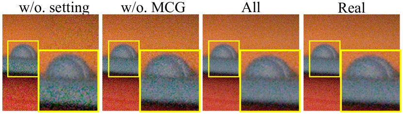
Figure 6: Results under ablation experiment settings.

Qualitative Comparison

Visual Analysis of Noisy Images.

We assess the subjective quality of synthetic noise by comparing RNSD with baselines such as C2N  (Jang et al. 2021) and sRGB2Flow (Kousha et al. 2022), as illustrated in Fig. 4. Across various camera sensors and ISO parameters, RNSD generates outputs that accurately resemble real-world noise patterns. This performance surpasses baseline methods which frequently struggle to capture high variance in noise distributions at larger noise levels.

Further, Fig. 7 shows our method’s controllability and necessity in incorporating camera settings like ISO. As we gradually adjust the ISO level, the noise in the synthesized images increases correspondingly. This confirms that RNSD can guide the model to synthesize more realistic noise and control the noise form by adjusting camera parameters.

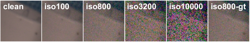
Figure 7: Illustration of noise synthesis results with varying ISO levels.

Metrics	CBDNet	ULRD	GRDN	C2N	sRGB2Flow	DANet	PNGAN	RNSD
AKLD$\downarrow$	0.728	0.545	0.443	0.314	0.237	0.212	0.153	0.126
PGap$\downarrow$	8.30	4.90	2.28	6.85	6.3	2.06	0.84	0.54

Table 2: The AKLD and PGap performances of different compared methods on the SIDD validation data set.

Quantitative Comparison

Method	C2N	N2F	R2F	GMDCN	RNSD	Real
PSNR$\uparrow$	33.98	33.81	34.74	36.07	37.95	38.34

Table 3: Denoising performance comparison between DnCNN trained on purely synthetic noise data and baseline.

Noise Generation.

We quantitatively evaluate our approach RNSD using the PGAP and AKLD metrics. We compare RNSD with several baseline techniques including CBDNet (Guo et al. 2019) , ULRD (Brooks et al. 2019) , GRDN (Kim, Chung, and Jung 2019) , C2N (Jang et al. 2021), sRGB2Flow (Kousha et al. 2022), DANet (Yue et al. 2020) , and PNGAN (Cai et al. 2021) on the SIDD dataset  (Abdelhamed, Lin, and Brown 2018), as show in Tab. 2. Our method outperforms the state-of-the-art (SOTA) in both metrics, with a PGAP lower by 0.20 and an improved AKLD by 0.027, indicating more stable results and a closer similarity to real-world noise.

Train from Scratch with Purely Synthetic Noise.

We train the DnCNN network (Zhang et al. 2017) from scratch using synthetic noise data generated by RNSD and compare its performance with baseline methods, including C2N (Jang et al. 2021), N2F(Noise Flow) (Abdelhamed, Brubaker, and Brown 2019), R2F(sRGB2Flow) (Kousha et al. 2022), GMDCN (Song et al. 2023). Our synthetic samples significantly improve denoising performance of DnCNN, with a PSNR improvement of 1.42dB over the current SOTA synthetic noise generation method, as depicted in Tab. 3. The PSNR performance of our DnCNN model, trained with synthetic noise, is 37.95dB, closely matching that of a model trained with real-world noise data (38.34dB).

Enhance Denoising Performance with Data Augmentation.

To evaluate the enhancement of synthetic data methods on actual denoising models, we select several commonly used denoising baselines, including DnCNN-B  (Zhang et al. 2017), RIDNet (Anwar and Barnes 2019), and NAFNet (Chen et al. 2022a). We assess the effects during the data augmentation process under different training dataset settings, except for the last experimental setting, where models are trained from scratch. The selected training dataset settings are as follows: only SIDD small dataset, SIDD small dataset and synthesized dataset with sRGB2Flow method, SIDD small dataset and synthesized dataset using RNSD, SIDD medium dataset, finetuning the baseline pretrained models using the SIDD medium dataset and our synthesized dataset. It is worth mentioning that our synthetic data model is only trained on the SIDD small dataset.

All our synthetic noise data samples are sourced from the clean images in the SIDD small dataset and the high-quality samples in the LSDIR dataset. As shown in Tab. 1, compared to using only the SIDD small dataset, our synthesized noise can further improve the PSNR and SSIM of all models. Our two-stage training also achieves better results than directly using the SIDD medium dataset. This is mainly due to two aspects: first, our synthesis method increases the diversity of noise distributions; second, the additional samples from the LSDIR dataset increase the content diversity. These two aspects enhance the generalization capability of the denoising models. And this fully validates that training image denoising networks with the high-quality noise data synthesized by RNSD can significantly improve the denoising performance of various networks.

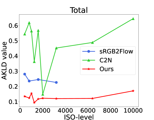
Figure 8: AKLD curves across various ISO levels for all images.

Performance Evaluation Across Different Camera Settings.

In order to evaluate the performance of RNSD across different camera settings, we consider ISO settings as an example. Fig. 8 shows that our noise synthesis method outperforms sRGB2Flow and C2N in terms of lower AKLD values across all ISO levels. This indicates our method’s capability to effectively capture significant noise distribution variations and learn a more realistic noise model. For comparisons under other camera settings, please refer to the supplementary material.

Method	AKLD$\downarrow$
Baseline	0.169
+ concat camera settings	0.137
+ CamSampler	0.130
+ MCG w/o. CamSampler	0.134
+ MCG w/ CamSampler	0.126

Table 4: Ablation study of the CamSampler mechanism and Multi-scale content guided structure.

Ablation Studies

Camera Settings.

We validate the effectiveness of integrating camera settings into our noise synthesis process. As demonstrated in Tab. 4, by concatenating camera settings to the input, the AKLD reduces from 0.169 (baseline UNet without camera conditions) to 0.137. Our proposed CamSampler technique, which uses an MLP to encode the camera settings together with the sampling steps instead of a simple concatenation with the condition tensor, reduces the AKLD to 0.130 further. This points to the effectiveness of CamSampler in generating adaptive noise patterns that conform better to given configurations, leading to higher fidelity synthetic noise.

We validate the effect of CamPredictor by training RIDNet from scratch using the SIDD small training set and augmented data synthesized from the LSDIR dataset. The noise data is synthesized using either randomly generated or CamPredictor predicted camera settings. As shown in Tab. 5, RIDNet trained with data from CamPredictor predicted settings achieves 0.21dB higher PSNR compared to using random settings. This demonstrates ability of CamPredictor to predict settings conforming better to scene characteristics and synthesize higher quality, more realistic noise.

Method	Baseline	CamPredictor
PSNR/SSIM	38.26/0.946	38.47/0.949

Table 5: Ablation study of the CamPredictor

Multi-scale content guided.

We examine the impact of our proposed MCG module. While the MCG module without CamSampler gives an AKLD of 0.134, using both MCG and CamSampler further reduces the AKLD to 0.126. This superior performance confirms the effectiveness of MCG in decoupling content and camera representations for guided noise synthesis.

Conclusion

In this paper, we introduce a novel method RNSD for synthesizing real noise based on diffusion for the first time. Camera setting information is encoded into the sampling step dimension to ensure the stability of our method during training and the controllability of its results. Dual multiscale encoders guide the generation of multi-frequency spatially correlated noise that matches real noise. Additionally, our designed inversion mechanism for the setting allows our method to have better scalability. We achieve state-of-the-art performance on multiple benchmarks and metrics, demonstrating the efficacy of our method. Moreover, in experiments with denoising models, we show that our synthesized data can significantly improve their denoising performance and generalization ability.

References

- Abdelhamed, Brubaker, and Brown (2019) Abdelhamed, A.; Brubaker, M. A.; and Brown, M. S. 2019. Noise flow: Noise modeling with conditional normalizing flows. In Proc. ICCV, 3165–3173.
- Abdelhamed, Lin, and Brown (2018) Abdelhamed, A.; Lin, S.; and Brown, M. S. 2018. A high-quality denoising dataset for smartphone cameras. In Proc. CVPR, 1692–1700.
- Anwar and Barnes (2019) Anwar, S.; and Barnes, N. 2019. Real image denoising with feature attention. In Proc. ICCV, 3155–3164.
- Bansal et al. (2022) Bansal, A.; Borgnia, E.; Chu, H.-M.; Li, J. S.; Kazemi, H.; Huang, F.; Goldblum, M.; Geiping, J.; and Goldstein, T. 2022. Cold diffusion: Inverting arbitrary image transforms without noise. arXiv preprint arXiv:2208.09392.
- Brock, Donahue, and Simonyan (2018) Brock, A.; Donahue, J.; and Simonyan, K. 2018. Large scale GAN training for high fidelity natural image synthesis. arXiv preprint arXiv:1809.11096.
- Brooks et al. (2019) Brooks, T.; Mildenhall, B.; Xue, T.; Chen, J.; Sharlet, D.; and Barron, J. T. 2019. Unprocessing images for learned raw denoising. In Proc. CVPR, 11036–11045.
- Cai et al. (2021) Cai, Y.; Hu, X.; Wang, H.; Zhang, Y.; Pfister, H.; and Wei, D. 2021. Learning to generate realistic noisy images via pixel-level noise-aware adversarial training. Proc. NeurIPS, 34: 3259–3270.
- Chen et al. (2022a) Chen, L.; Chu, X.; Zhang, X.; and Sun, J. 2022a. Simple Baselines for Image Restoration. In Proc. ECCV, 17–33.
- Chen et al. (2022b) Chen, S.; Sun, P.; Song, Y.; and Luo, P. 2022b. Diffusiondet: Diffusion model for object detection. arXiv preprint arXiv:2211.09788.
- Foi (2009) Foi, A. 2009. Clipped noisy images: Heteroskedastic modeling and practical denoising. Signal Processing, 89(12): 2609–2629.
- Foi et al. (2008) Foi, A.; Trimeche, M.; Katkovnik, V.; and Egiazarian, K. 2008. Practical Poissonian-Gaussian noise modeling and fitting for single-image raw-data. IEEE Trans. on Image Processing, 17(10): 1737–1754.
- Guo et al. (2019) Guo, S.; Yan, Z.; Zhang, K.; Zuo, W.; and Zhang, L. 2019. Toward convolutional blind denoising of real photographs. In Proc. CVPR, 1712–1722.
- He et al. (2016) He, K.; Zhang, X.; Ren, S.; and Sun, J. 2016. Deep Residual Learning for Image Recognition. In Proc. CVPR, 770–778.
- Ho, Jain, and Abbeel (2020) Ho, J.; Jain, A.; and Abbeel, P. 2020. Denoising diffusion probabilistic models. Proc. NeurIPS, 33: 6840–6851.
- Jang et al. (2021) Jang, G.; Lee, W.; Son, S.; and Lee, K. M. 2021. C2n: Practical generative noise modeling for real-world denoising. In Proc. CVPR, 2350–2359.
- Karras et al. (2017) Karras, T.; Aila, T.; Laine, S.; and Lehtinen, J. 2017. Progressive growing of gans for improved quality, stability, and variation. arXiv preprint arXiv:1710.10196.
- Karras, Laine, and Aila (2019) Karras, T.; Laine, S.; and Aila, T. 2019. A style-based generator architecture for generative adversarial networks. In Proc. CVPR, 4401–4410.
- Kim, Chung, and Jung (2019) Kim, D.-W.; Chung, J. R.; and Jung, S.-W. 2019. GRDN:Grouped Residual Dense Network for Real Image Denoising and GAN-based Real-world Noise Modeling. In Proc. CVPRW, 0–0.
- Kim et al. (2020) Kim, Y.; Soh, J. W.; Park, G. Y.; and Cho, N. I. 2020. Transfer learning from synthetic to real-noise denoising with adaptive instance normalization. In Proc. CVPR, 3482–3492.
- Kousha et al. (2022) Kousha, S.; Maleky, A.; Brown, M. S.; and Brubaker, M. A. 2022. Modeling srgb camera noise with normalizing flows. In Proc. CVPR, 17463–17471.
- Li et al. (2023) Li, Y.; Zhang, K.; Liang, J.; Cao, J.; Liu, C.; Gong, R.; Zhang, Y.; Tang, H.; Liu, Y.; Demandolx, D.; Ranjan, R.; Timofte, R.; and Van Gool, L. 2023. LSDIR Dataset: A Large Scale Dataset for Image Restoration.
- Nam et al. (2016) Nam, S.; Hwang, Y.; Matsushita, Y.; and Kim, S. J. 2016. A holistic approach to cross-channel image noise modeling and its application to image denoising. In Proc. CVPR, 1683–1691.
- Plotz and Roth (2017) Plotz, T.; and Roth, S. 2017. Benchmarking denoising algorithms with real photographs. In Proc. CVPR, 1586–1595.
- San-Roman, Nachmani, and Wolf (2021) San-Roman, R.; Nachmani, E.; and Wolf, L. 2021. Noise estimation for generative diffusion models. arXiv preprint arXiv:2104.02600.
- Shaham, Dekel, and Michaeli (2019) Shaham, T. R.; Dekel, T.; and Michaeli, T. 2019. Singan: Learning a generative model from a single natural image. In Proc. CVPR, 4570–4580.
- Song, Meng, and Ermon (2020) Song, J.; Meng, C.; and Ermon, S. 2020. Denoising diffusion implicit models. arXiv preprint arXiv:2010.02502.
- Song et al. (2023) Song, M.; Zhang, Y.; Aydın, T. O.; Mansour, E. A.; and Schroers, C. 2023. A Generative Model for Digital Camera Noise Synthesis.
- Wang et al. (2022) Wang, Z.; Cun, X.; Bao, J.; Zhou, W.; Liu, J.; and Li, H. 2022. Uformer: A General U-Shaped Transformer for Image Restoration. In Proc. CVPR, 17683–17693.
- Xing, Qian, and Chen (2021) Xing, Y.; Qian, Z.; and Chen, Q. 2021. Invertible Image Signal Processing. In Proc. CVPR.
- Xu et al. (2018) Xu, J.; Li, H.; Liang, Z.; Zhang, D.; and Zhang, L. 2018. Real-world noisy image denoising: A new benchmark. arXiv preprint arXiv:1804.02603.
- Yue et al. (2020) Yue, Z.; Zhao, Q.; Zhang, L.; and Meng, D. 2020. Dual Adversarial Network: Toward Real-world Noise Removal and Noise Generation. In Proc. ECCV, 41–58.
- Zamir et al. (2022) Zamir, S. W.; Arora, A.; Khan, S.; Hayat, M.; Khan, F. S.; and Yang, M.-H. 2022. Restormer: Efficient Transformer for High-Resolution Image Restoration. In Proc. CVPR, 5728–5739.
- Zamir et al. (2020) Zamir, S. W.; Arora, A.; Khan, S.; Hayat, M.; Khan, F. S.; Yang, M.-H.; and Shao, L. 2020. Cycleisp: Real image restoration via improved data synthesis. In Proc. CVPR, 2696–2705.
- Zamir et al. (2021) Zamir, S. W.; Arora, A.; Khan, S.; Hayat, M.; Khan, F. S.; Yang, M.-H.; and Shao, L. 2021. Multi-stage progressive image restoration. In Proc. CVPR, 14821–14831.
- Zhang et al. (2017) Zhang, K.; Zuo, W.; Chen, Y.; Meng, D.; and Zhang, L. 2017. Beyond a Gaussian Denoiser: Residual Learning of Deep CNN for Image Denoising. In IEEE Trans. on Image Processing, 3142–3155.
- Zhang, Zuo, and Zhang (2018) Zhang, K.; Zuo, W.; and Zhang, L. 2018. FFDNet: Toward a fast and flexible solution for CNN-based image denoising. IEEE Trans. on Image Processing, 27(9): 4608–4622.
- Zhou et al. (2020) Zhou, Y.; Jiao, J.; Huang, H.; Wang, Y.; Wang, J.; Shi, H.; and Huang, T. 2020. When awgn-based denoiser meets real noises. In Proc. AAAI, volume 34, 13074–13081.