Expressive Losses for Verified Robustness
via Convex Combinations

Abstract

In order to train networks for verified adversarial robustness, previous work typically over-approximates the worst-case loss over (subsets of) perturbation regions or induces verifiability on top of adversarial training. The key to state-of-the-art performance lies in the expressivity of the employed loss function, which should be able to match the tightness of the verifiers to be employed post-training. We formalize a definition of expressivity, and show that it can be satisfied via simple convex combinations between adversarial attacks and IBP bounds. We then show that the resulting algorithms, named CC-IBP and MTL-IBP, yield state-of-the-art results across a variety of settings in spite of their conceptual simplicity. In particular, for $\ell_{\infty}$ perturbations of radius $\nicefrac{{1}}{{255}}$ on TinyImageNet and downscaled ImageNet, MTL-IBP improves on the best standard and verified accuracies from the literature by from $1.98\%$ to $3.92\%$ points while only relying on single-step adversarial attacks.

1 Introduction

In spite of recent and highly-publicized successes [34, 24, 50], serious concerns over the trustworthiness of deep learning systems remain. In particular, the vulnerability of neural networks to adversarial examples [64, 26] questions their applicability to safety-critical domains. As a result, many authors devised techniques to formally prove the adversarial robustness of trained neural networks [43, 22, 35]. Either implicitly or explicitly, these algorithms solve a non-convex optimization problem by coupling network over-approximations with search techniques [8]. While the use of network verifiers was initially limited to models with hundreds of neurons, the scalability of these tools has steadily increased over the recent years [9, 6, 28, 75, 18, 68, 29, 25], reaching networks of the size of VGG16 [55, 47]. Nevertheless, significant gaps between state-of-the-art verified and empirical robustness persist, the latter referring to specific adversarial attacks. For instance, on ImageNet [20], Singh et al. [59] attain an empirical robustness of $57.70\%$ to $\ell_{\infty}$ perturbations of radius $\epsilon=\nicefrac{{4}}{{255}}$, whereas the state-of-the-art verified robust accuracy (on a downscaled version of the dataset [12]) is $9.54\%$ against $\epsilon=\nicefrac{{1}}{{255}}$ [79]. In fact, while empirical robustness can be achieved by training the networks against relatively inexpensive attacks (adversarial training) [44, 71], the resulting networks remain hard to verify as their over-approximations are typically loose.

In order to train networks amenable to formal robustness verification (verified training), a number of works [46, 27, 69, 70, 81, 74, 54] directly compute the loss over the network over-approximations that are later used for formal verification (verified loss). The employed approximations are typically loose, as the difficulty of the optimization problem associated with training increases with approximation tightness, resulting in losses that are hard to train against [41, 33]. As a result, while the resulting models are easy to verify, these networks display sub-par standard accuracy. Another line of work enhances adversarial training with verifiability-inducing techniques [72, 5, 19]: by exploiting stronger verifiers, these algorithms yield better results against small perturbations, but under-perform in other settings. A recent work, SABR [49], combined the advantages of both strategies by computing the loss on over-approximations of small “boxes" around adversarial attacks. Larger boxes correspond to increased IBP-verified robust accuracy and decreased standard performance: by tuning the size of these boxes on each setting, Müller et al. [49] demonstrate that SABR attains state-of-the-art performance.

The ability of a loss function to mirror the degree of over-approximation employed at verification time is the key to effective verified training schemes [49, 45]. While simple convex combinations between adversarial attacks and IBP bounds are expressive enough to capture a wide range of approximations, their use has been under-explored in previous work. Aiming to fill this gap, we present the following contributions:

• Inspired by SABR, we define a general class of loss functions (definition 3.1), which we call expressive, that go from the adversarial to the verified loss when increasing a single parameter $\alpha$ from $0$ to $1$.

• We show how expressive losses can be easily designed via convex combinations, and present two examples: (i) CC-IBP, which takes combinations between adversarial and over-approximated network outputs within the loss, (ii) MTL-IBP, which relies on combinations between the adversarial and verified losses, lending itself to a multi-task [11] interpretation.

• We present a comprehensive experimental evaluation of CC-IBP and MTL-IBP on benchmarks from the robust vision literature. In spite of their conceptual simplicity, both methods attain state-of-the-art performance, either matching or improving upon the reported results of SABR and its very recent follow-up [45] on all the considered settings. Improvements upon literature results are relatively large on TinyImageNet [39] and downscaled ($64\times 64$) ImageNet [12], where MTL-IBP improves on both standard and verified robust accuracy by at least $1.98\%$ points. Furthermore, both algorithms perform well under a single-step adversarial attack [71], thus only adding minimal overhead compared to standard IBP training.

2 Background

We employ the following notation: uppercase letters for matrices (for example, $A$), boldface letters for vectors (for example, $\bf{a}$), brackets for intervals and vector indices ($[\bf{a},\bf{b}]$ and $\mathbf{a}[i]$, respectively), $\odot$ for the Hadamard product, $\llbracket\cdot\rrbracket$ for integer ranges, $[\mathbf{a}]_{+}:=\max(\mathbf{a},\mathbf{0})$ and $[\mathbf{a}]_{-}:=\min(\mathbf{a},\mathbf{0})$.

Let $f:\mathbb{R}^{S}\times\mathbb{R}^{d}\rightarrow\mathbb{R}^{o}$ be a neural network with parameters $\bm{\theta}\in\mathbb{R}^{S}$ and accepting $d$-dimensional inputs. Given a dataset $(\mathbf{x},\mathbf{y})\sim\mathcal{D}$ with points $\mathbf{x}\in\mathbb{R}^{d}$ and labels $\mathbf{y}\in\mathbb{R}^{l}$, the goal of robust training is to obtain a network that satisfies a given property $P:\mathbb{R}^{o}\times\mathbb{R}^{l}\rightarrow\{0,1\}$ on $\mathcal{D}$:

$$(\mathbf{x},\mathbf{y})\sim\mathcal{D}\ \implies P(f(\bm{\theta},\mathbf{x}),\mathbf{y}).$$

We will focus on classification problems, with scalar labels $y\in\mathbb{R}$, and on verifying robustness to adversarial perturbations around the inputs. Defining $\mathbf{z}(\bm{\theta},\mathbf{x},y):=\left(\mathbf{1}\odot f(\bm{\theta},\mathbf{x})[y]-f(\bm{\theta},\mathbf{x})\right)$ and given a perturbation domain $\mathcal{C}(\mathbf{x},\epsilon):=\{\mathbf{x}_{0}:\left\lVert\mathbf{x}_{0}-\mathbf{x}\right\rVert_{p}\leq\epsilon\}$, we can write:

$$P(f(\bm{\theta},\mathbf{x}),y)=\left[\left(\operatorname*{\arg\!\min}_{i\neq y}\mathbf{z}(\bm{\theta},\mathbf{x},y)[i]>0\right)\forall\ \mathbf{x}_{0}\in\mathcal{C}(\mathbf{x},\epsilon)\right].$$ (1)

2.1 Adversarial Training

Given a loss function $\mathcal{L}:\mathbb{R}^{o}\times\mathbb{R}^{l}\rightarrow\mathbb{R}$, a network is typically trained by optimizing $\min_{\bm{\theta}}\ \operatorname*{\mathbb{E}}_{(\mathbf{x},\mathbf{y})\in\mathcal{D}}\left[\mathcal{L}(f(\bm{\theta},\mathbf{x}),\mathbf{y})\right]$ through variants of Stochastic Gradient Descent (SGD). Hence, training for adversarial robustness requires a surrogate loss adequately representing equation (1). Borrowing from the robust optimization literature, Madry et al. [44] introduce the so-called robust loss:

$$\mathcal{L}^{*}(f(\bm{\theta},\mathbf{x}),y):=\max_{\mathbf{x}^{\prime}\in\mathcal{C}(\mathbf{x},\epsilon)}\mathcal{L}(f(\bm{\theta},\mathbf{x}^{\prime}),y).$$ (2)

However, given the non-convexity of the maximization problem, Madry et al. [44] propose to approximate its computation by a lower bound, which is obtained via a local optimizer (adversarial attack). Denoting by $\mathbf{x}_{\text{adv}}\in\mathcal{C}(\mathbf{x},\epsilon)$ the point returned by the attack, the adversarial loss is defined as follows:

$$\mathcal{L}_{\text{adv}}(f(\bm{\theta},\mathbf{x}),y):=\mathcal{L}(f(\bm{\theta},\mathbf{x}_{\text{adv}}),y)\leq\mathcal{L}^{*}(f(\bm{\theta},\mathbf{x}),y).$$ (3)

Adversarially trained models typically display strong empirical robustness to adversarial attacks and a reduced standard accuracy compared to models not trained for robustness. However, formal verification methods fail to formally prove their robustness in a feasible time [72]. Furthermore, as repeatedly shown in the past [67, 3], these defenses may break under stronger or conceptually different attacks [14]. As a result, a number of algorithms have been designed to make networks more amenable to formal verification.

2.2 Training for Verified Robustness

As seen from equation (1), a network is provably robust if one can show that all logit differences $\mathbf{z}(\bm{\theta},\mathbf{x},y)$, except the one corresponding to the ground truth, are positive over $\mathcal{C}(\mathbf{x},\epsilon)$.

2.2.1 Neural Network Verification

Formal verification amounts to computing the sign of the following optimization problem:

$$\smash{\min_{\mathbf{x}_{0}}}\quad\operatorname*{\arg\!\min}_{i\neq y}\mathbf{z}(\bm{\theta},\mathbf{x}_{0},y)[i]\qquad\text{s.t. }\qquad\mathbf{x}_{0}\in\mathcal{C}(\mathbf{x},\epsilon)$$ (4)

Problem (4) is known to be NP-hard [35]. Indeed, solving it is as hard as exactly computing the robust loss from equation (2). Therefore, it is typically replaced by more tractable lower bounds (incomplete verification): if the bound is positive, then the network is proved to be robust. Incomplete verifiers will only prove a subset of the properties, with tighter approximations leaving fewer properties undecided.

Figure 1: IBP ReLU over-approximation, with $\hat{x}\in[\hat{l},\hat{u}]$ for the considered input domain.

Let us denote lower bounds to the logit differences by:

$$\underaccent{\bar}{\zb}(\bm{\theta},\mathbf{x},y)\leq\mathbf{z}(\bm{\theta},\mathbf{x}_{0},y)\ \forall\ \mathbf{x}_{0}\in\mathcal{C}(\mathbf{x},\epsilon).$$

Furthermore, let $W_{k}$ be the weight matrix of the $k$-th layer of the network, and $\mathbf{b}_{k}$ its bias. An immediate application of interval arithmetic [63, 30] to neural networks, Interval Bound Propagation (IBP) [27, 46], provides a popular and inexpensive incomplete verifier. For a $n$-layer ReLU network, it computes $\underaccent{\bar}{\zb}(\bm{\theta},\mathbf{x},y)$ as $\hat{\mathbf{l}}_{n}$ from the following iterative procedure:

$$\begin{array}[]{r}\hat{\mathbf{l}}_{1}=\max_{\mathbf{x}_{0}\in\mathcal{C}(\mathbf{x},\epsilon)}W_{1}\mathbf{x}_{0}+\mathbf{b}_{1}\\ \hat{\mathbf{u}}_{1}=\min_{\mathbf{x}_{0}\in\mathcal{C}(\mathbf{x},\epsilon)}W_{1}\mathbf{x}_{0}+\mathbf{b}_{1}\end{array}\enskip\left\{\begin{array}[]{r}\hat{\mathbf{u}}_{k}=\left[W_{k}\right]_{+}[\hat{\mathbf{u}}_{k-1}]_{+}+[W_{k}]_{-}[\hat{\mathbf{l}}_{k-1}]_{+}+\mathbf{b}_{k}\\ \hat{\mathbf{l}}_{k}=\left[W_{k}\right]_{+}[\hat{\mathbf{l}}_{k-1}]_{+}+[W_{k}]_{-}[\hat{\mathbf{u}}_{k-1}]_{+}+\mathbf{b}_{k}\end{array}\right\}\ k\in\left\llbracket 1,n\right\rrbracket.$$

IBP corresponds to solving an approximation of problem (4) where all the network layers are replaced by their bounding boxes. For instance, given some $\hat{l}$ and $\hat{u}$ from the above procedure, the ReLUs are replaced by the over-approximation depicted in figure 1. The cost of computing $\underaccent{\bar}{\zb}(\bm{\theta},\mathbf{x},y)$ via IBP roughly corresponds to four network evaluations.

If an exact solution to (the sign of) problem (4) is required, incomplete verifiers can be plugged in into a branch-and-bound framework [8, 10]. These algorithms provide an answer on any given property (complete verification) by recursively splitting the optimization domain (branching), and computing bounds to the solutions of the sub-problems. Lower bounds are obtained via incomplete verifiers, whereas adversarial attacks ($\S$2.1) provide upper bounds. For ReLU activations and high-dimensional input spaces, branching is typically performed implicitly by splitting a ReLU into its two linear pieces [18, 25].

2.2.2 Training Methods

The verified training literature commonly employs the following assumption [69, 81]:

Assumption 2.1.

The loss function $\mathcal{L}$ is translation-invariant: $\mathcal{L}(-\mathbf{z}(\bm{\theta},\mathbf{x},y),y)=\mathcal{L}(f(\bm{\theta},\mathbf{x}),y)$). Furthermore, $\mathcal{L}(-\mathbf{z}(\bm{\theta},\mathbf{x},y),y)$ is monotonic increasing with respect to $-\mathbf{z}(\bm{\theta},\mathbf{x}_{0},y)[i]$ if $i\neq y$.

Assumption 2.1 holds for popular loss functions such as cross-entropy. In this case, one can provide an upper bound to the robust loss $\mathcal{L}^{*}$ via the so-called verified loss $\mathcal{L}_{\text{ver}}(f(\bm{\theta},\mathbf{x}),y)$, computed on a lower bound to the logit differences $\underaccent{\bar}{\zb}(\bm{\theta},\mathbf{x},y)$ obtained from an incomplete verifier [69]:

$$\mathcal{L}^{*}(f(\bm{\theta},\mathbf{x}),y)\leq\mathcal{L}_{\text{ver}}(f(\bm{\theta},\mathbf{x}),y):=\mathcal{L}(-\underaccent{\bar}{\zb}(\bm{\theta},\mathbf{x},y),y).$$ (5)

A number of verified training algorithms employ a loss of the form $\mathcal{L}_{\text{ver}}(f(\bm{\theta},\mathbf{x}),y)$ above as fundamental component, where bounds $-\underaccent{\bar}{\zb}(\bm{\theta},\mathbf{x},y)$ are obtained via IBP [27, 54], inexpensive linear relaxations [69], or a mixture of the two [81]. In order to stabilize training, the radius of the perturbation over which the bounds are computed is gradually increased from $0$ to the target $\epsilon$ value (ramp-up). Furthermore, earlier approaches [27, 81] may linearly transition from the natural to the robust loss: $(1-\kappa)\ \mathcal{L}(f(\bm{\theta},\mathbf{x}),y)+\kappa\ \mathcal{L}_{\text{ver}}(f(\bm{\theta},\mathbf{x}),y)$, with $\kappa$ linearly increasing from $0$ to $0.5$ or $1$ during ramp-up. Zhang et al. [81] may further transition from lower bounds $\underaccent{\bar}{\zb}(\bm{\theta},\mathbf{x},y)$ partly obtained via linear relaxations (CROWN-IBP) to IBP bounds within $\mathcal{L}_{\text{ver}}(f(\bm{\theta},\mathbf{x}),y)$: $(1-\kappa)\ \mathcal{L}(f(\bm{\theta},\mathbf{x}),y)+\kappa\ \mathcal{L}(-\left((1-\beta)\ \underaccent{\bar}{\zb}_{\text{IBP}}(\bm{\theta},\mathbf{x},y)+\beta\ \underaccent{\bar}{\zb}_{\text{CROWN-IBP}}(\bm{\theta},\mathbf{x},y)\right),y)$, with $\beta$ linearly increased from $0$ to $1$. A more recent method [54] removes both transitions and significantly reduces training times by employing BatchNorm [32] along with specialized initialization and regularization. These algorithms attain strong verified adversarial robustness, verifiable via inexpensive incomplete verifiers, while paying a relatively large price in standard accuracy.

Another line of research tries to reduce the impact on standard accuracy by relying on stronger verifiers and coupling adversarial training ($\S$2.1) with verifiability-inducing techniques. Examples include maximizing network local linearity [72], performing the attacks in the latent space over network over-approximations (COLT) [5], and minimizing the area of over-approximations used at verification time while attacking over larger input regions (IBP-R) [19]. In most cases $\ell_{1}$ regularization was found to be beneficial. A more recent work, named SABR [49], proposes to compute bounds via IBP over a parametrized subset of the input domain that includes an adversarial attack. Let us denote by $\text{Proj}(\mathbf{a},\mathcal{A})$ the Euclidean projection of $\mathbf{a}$ on set $\mathcal{A}$. Given $\mathbf{x}_{\lambda}:=\text{Proj}(\mathbf{x}_{\text{adv}},\mathcal{C}(\mathbf{x},\epsilon-\lambda\epsilon))$, SABR relies on the following loss:

$$\mathcal{L}(-\underaccent{\bar}{\zb}_{\lambda}(\bm{\theta},\mathbf{x},y),y)\text{, where}\enskip\underaccent{\bar}{\zb}_{\lambda}(\bm{\theta},\mathbf{x},y)\leq\mathbf{z}(\bm{\theta},\mathbf{x}_{0},y)\enskip\forall\ \mathbf{x}_{0}\in\mathcal{C}(\mathbf{x}_{\lambda},\lambda\epsilon)\subseteq\mathcal{C}(\mathbf{x},\epsilon).$$ (6)

The SABR loss is not necessarily an upper bound for $\mathcal{L}^{*}(f(\bm{\theta},\mathbf{x}),y)$. However, it continuously interpolates between $\mathcal{L}(f(\bm{\theta},\mathbf{x}_{\text{adv}}),y)$, which it matches when $\lambda=0$, and $\mathcal{L}_{\text{ver}}(f(\bm{\theta},\mathbf{x}),y)$, matched when $\lambda=1$. By tuning $\lambda\in[0,1]$, SABR attains state-of-the-art performance under complete verifiers [49]. A very recent follow-up work, named STAPS [45], combines SABR with improvements on COLT, further improving its performance on some benchmarks at the cost of added complexity.

3 Convex Combinations for Verified Training

We define a class of loss functions, which we call expressive, that, through the value of a single parameter $\alpha$, range between the adversarial loss in equation (3) to the verified loss in equation (5):

Definition 3.1.

A parametrized family of losses $\mathcal{L}_{\alpha}(\bm{\theta},\mathbf{x},y)$ is expressive if:

• $\mathcal{L}(f(\bm{\theta},\mathbf{x}_{\text{adv}}),y)\leq\mathcal{L}_{\alpha}(\bm{\theta},\mathbf{x},y)\leq\mathcal{L}_{\text{ver}}(f(\bm{\theta},\mathbf{x}),y)\ \forall\ \alpha\in[0,1]$;

• $\mathcal{L}_{\alpha}(\bm{\theta},\mathbf{x},y)$ is monotonically increasing with $\alpha$;

• $\mathcal{L}_{0}(\bm{\theta},\mathbf{x},y)=\mathcal{L}(f(\bm{\theta},\mathbf{x}_{\text{adv}}),y)$;

• $\mathcal{L}_{1}(\bm{\theta},\mathbf{x},y)=\mathcal{L}_{\text{ver}}(f(\bm{\theta},\mathbf{x}),y)$.

Intuitively, if a network is trained on $\mathcal{L}_{\alpha}(\bm{\theta},\mathbf{x},y)<<\mathcal{L}^{*}(f(\bm{\theta},\mathbf{x}),y)$, verified robustness will be hard to achieve via any complete verifier. However, if $\mathcal{L}_{\alpha}(\bm{\theta},\mathbf{x},y)\approxeq\mathcal{L}_{\text{ver}}(f(\bm{\theta},\mathbf{x}),y)$, with $\underaccent{\bar}{\zb}(\bm{\theta},\mathbf{x},y)$ obtained via a loose incomplete verifier, robustness will be easier to verify, but it will come at a high cost in standard accuracy. Finally, if $\mathcal{L}_{\alpha}(\bm{\theta},\mathbf{x},y)\approxeq\mathcal{L}^{*}(f(\bm{\theta},\mathbf{x}),y)$, verification will be guaranteed only if computing the true $\mathcal{L}^{*}(f(\bm{\theta},\mathbf{x}),y)$, which is intractable (see $\S$2.2.1). In general, the most effective $\alpha$ will depend on the problem at hand. Motivated by the performance of SABR [49], whose loss from equation (6) satisfies definition 3.1 when setting $\lambda=\alpha$ (see appendix B), we believe expressivity to be crucial in order to attain state-of-the-art verified adversarial robustness.

Using definition 3.1 as design principle, we now present two simple ways to obtain expressive loss families through convex combinations between adversarial attacks and bounds from incomplete verifiers.

3.1 CC-IBP

A family of expressive losses can be easily obtained by taking Convex Combinations (CC) of adversarial and lower bounds to logit differences within the loss function:

$$\mathcal{L}_{\alpha,\text{CC}}(\bm{\theta},\mathbf{x},y):=\mathcal{L}(-\left[(1-\alpha)\ \mathbf{z}(\bm{\theta},\mathbf{x}_{\text{adv}},y)+\alpha\ \underaccent{\bar}{\zb}(\bm{\theta},\mathbf{x},y)\right],y).$$ (7)

Proposition 3.2.

The parametrized loss $\mathcal{L}_{\alpha,\text{CC}}(\bm{\theta},\mathbf{x},y)$ is expressive according to definition 3.1.

Proof.

Trivially, $\mathcal{L}_{0,\text{CC}}(\bm{\theta},\mathbf{x},y)=\mathcal{L}(f(\bm{\theta},\mathbf{x}_{\text{adv}}),y)$, and $\mathcal{L}_{1,\text{CC}}(\bm{\theta},\mathbf{x},y)=\mathcal{L}_{\text{ver}}(f(\bm{\theta},\mathbf{x}),y)$. By definition $\underaccent{\bar}{\zb}(\bm{\theta},\mathbf{x},y)\leq\mathbf{z}(\bm{\theta},\mathbf{x}_{\text{adv}},y)$, as $\mathbf{x}_{\text{adv}}\in\mathcal{C}(\mathbf{x},\epsilon)$. Then, owing to assumption 2.1 and to $\mathbf{z}(\bm{\theta},\mathbf{x}_{\text{adv}},y)[y]=\underaccent{\bar}{\zb}(\bm{\theta},\mathbf{x},y)[y]=0$, as $\underaccent{\bar}{\zb}(\bm{\theta},\mathbf{x},y)\leq(1-\alpha)\ \mathbf{z}(\bm{\theta},\mathbf{x}_{\text{adv}},y)+\alpha\ \underaccent{\bar}{\zb}(\bm{\theta},\mathbf{x},y)\leq\mathbf{z}(\bm{\theta},\mathbf{x}_{\text{adv}},y)$ for $\alpha\in[0,1]$, $\mathcal{L}(f(\bm{\theta},\mathbf{x}_{\text{adv}}),y)\leq\mathcal{L}_{\alpha}(\bm{\theta},\mathbf{x},y)\leq\mathcal{L}_{\text{ver}}(f(\bm{\theta},\mathbf{x}),y)$, which concludes the proof. ∎

The analytical form of equation (7) when $\mathcal{L}$ is the cross-entropy loss, including a comparison to the loss from SABR, is presented in appendix C. In order to minimize computational costs and to yield favorable optimization problems [33], we employ IBP to compute $\underaccent{\bar}{\zb}(\bm{\theta},\mathbf{x},y)$, and refer to the resulting algorithm as CC-IBP. We remark that a similar convex combination was employed in the CROWN-IBP [81] loss (see $\S$2.2.2). However, while CROWN-IBP takes a combination between IBP and CROWN-IBP lower bounds to the logit differences, we replace the latter by logit differences associated to an adversarial attack. Furthermore, rather than increasing the combination coefficient from $0$ to $1$ during ramp-up, we propose to employ a constant and tunable $\alpha$ throughout training.

3.2 MTL-IBP

Convex combination can be also performed between loss functions $\mathcal{L}$, resulting in:

$$\mathcal{L}_{\alpha,\text{MTL}}(\bm{\theta},\mathbf{x},y):=(1-\alpha)\mathcal{L}(f(\bm{\theta},\mathbf{x}_{\text{adv}}),y)+\alpha\ \mathcal{L}_{\text{ver}}(f(\bm{\theta},\mathbf{x}),y).$$ (8)

The above loss lends itself to a Multi-Task Learning (MTL) interpretation [11], with empirical and verified adversarial robustness as the tasks. Under this view, borrowing terminology from multi-objective optimization, $\mathcal{L}_{\alpha,\text{MTL}}(\bm{\theta},\mathbf{x},y)$ amounts to a scalarization of the multi-task problem.

Proposition 3.3.

The parametrized loss $\mathcal{L}_{\alpha,\text{MTL}}(\bm{\theta},\mathbf{x},y)$ is expressive. Furthermore, if $\mathcal{L}(\cdot,y)$ is convex with respect to its first argument, $\mathcal{L}_{\alpha,\text{CC}}(\bm{\theta},\mathbf{x},y)\leq\mathcal{L}_{\alpha,\text{MTL}}(\bm{\theta},\mathbf{x},y)\ \forall\ \alpha\in[0,1]$.

Proof.

The proof for the first part of the statement closely follows the proof for proposition 3.2, while not requiring assumption 2.1. $\mathcal{L}_{\alpha,\text{CC}}(\bm{\theta},\mathbf{x},y)\leq\mathcal{L}_{\alpha,\text{MTL}}(\bm{\theta},\mathbf{x},y)\ \forall\ \alpha\in[0,1]$ trivially follows from the definition of a convex function [7, section 3.1.1] and equation (5). ∎

The second part of proposition 3.3, which applies to cross-entropy, relates the $\mathcal{L}_{\alpha,\text{MTL}}(\bm{\theta},\mathbf{x},y)$ and $\mathcal{L}_{\alpha,\text{CC}}(\bm{\theta},\mathbf{x},y)$ losses: the former can be seen as an upper bound to the latter for $\alpha\in[0,1]$. Owing to definition 3.1, the bound will be tight when $\alpha\in\{0,1\}$. Appendix C shows an analytical form for equation (8) when $\mathcal{L}$ is the cross-entropy loss. As in section 3.1, we use IBP to compute $\mathcal{L}_{\text{ver}}(f(\bm{\theta},\mathbf{x}),y)$; we refer to the resulting algorithm as MTL-IBP. Given its simplicity, ideas related to equation (8) have previously been adopted in the literature. For instance, Gowal et al. [27] take a convex combination between the natural loss (rather than adversarial) and the IBP loss; however, instead of tuning a constant $\alpha$, they linearly transition it from $0$ to $0.5$ during ramp-up (see $\S$2.2.2). Mirman et al. [46] employ $\mathcal{L}(f(\bm{\theta},\mathbf{x}_{\text{adv}}),y)+0.1\ \left(-\text{softplus}(\min_{i\neq y}\underaccent{\bar}{\zb}(\bm{\theta},\mathbf{x},y)[i])\right)$. The closely-related AdvIBP [23] also casts training as a multi-task problem between lower and upper bounds to the robust loss. However, it relies on a layer-wise scheme similar to COLT [5], and it explicitly argues against scalarizations, relying instead on a complex specialized multi-task optimizer. We instead opt for scalarizations, which, when appropriately tuned and regularized, have recently been shown to yield state-of-the-art results on multi-task benchmarks [37, 73].

4 Related Work

As outlined in $\S$2.2.2, many verified training algorithms work by either directly upper bounding the robust loss [27, 46, 69, 81, 74, 54], or by inducing verifiability on top of adversarial training [72, 5, 19, 49, 45]: this work falls in the latter category. Algorithms belonging to these classes are typically employed against $\ell_{\infty}$ perturbations. Other families of methods include Lipschitz-based regularization for $\ell_{2}$ perturbations [42, 31], and architectures that are designed to be inherently robust for either $\ell_{2}$ [66, 60, 62, 61, 76] or $\ell_{\infty}$ [77, 78] perturbations, for which SortNet [79] is the most recent and effective algorithm. A prominent line of work has focused on achieving robustness with high probability through randomization [13, 53]: we here focus on deterministic methods.

IBP, presented in $\S$2.2.1, is arguably the simplest incomplete verifier. A popular class of algorithms replaces the activation by over-approximations corresponding to pairs of linear bound, each respectively providing a lower or upper bound to the activation function [69, 56, 80, 58]. Tighter over-approximations can be obtained by representing the convex hull of the activation function [22, 9, 75], the convex hull of the composition of the activation with the preceding linear layer [2, 65, 16, 17], interactions within the same layer [57, 48], or by relying on semi-definite relaxations [52, 15, 38]. In general, the tighter the bounds, the more expensive their computation. As seen in the recent neural network verification competitions [4, 47], state-of-the-art complete verifiers based on branch-and-bound typically rely on specialized and massively-parallel incomplete verifiers [68, 25, 82], paired with custom branching heuristics [10, 18, 25].

5 Experimental Evaluation

We now present an experimental evaluation of CC-IBP and MTL-IBP ($\S$3) on commonly employed vision benchmarks. We first compare their performance with the existing literature ($\S$5.1), then show ablation studies on the employed attack ($\S$5.2) and on the post-training verification algorithm ($\S$5.3).

We implemented CC-IBP and MTL-IBP in PyTorch [51], starting from the publicly available training pipeline by Shi et al. [54], based on automatic LiRPA [74], and exploiting their specialized initialization and regularization techniques. All our experiments use the same 7-layer architecture as previous work [54, 49], which employs BatchNorm [32] after every layer. In order to minimize training overhead and unless otherwise stated, we rely on randomly-initialized FGSM [26, 71] to compute the attack point $\mathbf{x}_{\text{adv}}$ in equations (7) and (8), and force the points to be on the perturbation boundary via a large step size (see appendix F.2 for an ablation). Unless specified otherwise, the reported verified robust accuracies for CC-IBP and MTL-IBP are computed using branch-and-bound, with a setup similar to IBP-R [19]. Specifically, we use the OVAL framework [10, 18], with a variant of the UPB branching strategy [19] and $\alpha$-$\beta$-CROWN as the bounding algorithm [68] (see appendix D). Details pertaining to the employed datasets, hyper-parameters, network architectures, and computational setup are reported in appendix E.

5.1 Comparison with Previous Work

Table 1: Performance of different verified training algorithms under $\ell_{\infty}$ norm perturbations on MNIST, CIFAR-10, TinyImageNet and downscaled ($64\times 64$) ImageNet datasets. The entries corresponding to the best standard or verified robust accuracy for each perturbation radius are highlighted in bold. For the remaining entries, improvements on the literature performance of the best-performing ReLU-based architectures are underlined.

Dataset $\epsilon$ Method Source Standard acc. [%] Verified rob. acc. [%] Training time [s] MNIST $0.1$ CC-IBP this work $99.30$ $98.43$ $2.71\times 10^{3}$ MTL-IBP this work 99.25 $98.38$ $2.69\times 10^{3}$ TAPS Mao et al. [45] $99.19$ $98.39$ $4.26\times 10^{4}$ SABR Müller et al. [49] $99.23$ $98.22$ $1.22\times 10^{4}$ SortNet Zhang et al. [79] $99.01$ $98.14$ $1.59\times 10^{4}$ IBP Shi et al. [54] $98.84$ $97.95$ $2.14\times 10^{3}$ AdvIBP Fan and Li [23] $98.97$ $97.72$ $1.29\times 10^{5}$ CROWN-IBP Zhang et al. [81] $98.83$ $97.76$ / COLT Balunovic and Vechev [5] $99.2$ $97.1$ / $0.3$ CC-IBP this work $98.81$ 93.58 $2.71\times 10^{3}$ MTL-IBP this work 98.80 $93.62$ $2.72\times 10^{3}$ STAPS Mao et al. [45] $98.53$ $93.51$ $1.24\times 10^{4}$ SABR Müller et al. [49] $98.75$ $93.40$ $1.20\times 10^{4}$ SortNet Zhang et al. [79] $98.46$ $93.40$ $1.59\times 10^{4}$ IBP Shi et al. [54] $97.67$ $93.10$ $2.14\times 10^{3}$ AdvIBP Fan and Li [23] $98.42$ $91.77$ $1.29\times 10^{5}$ CROWN-IBP Zhang et al. [81] $98.18$ $92.98$ $5.58\times 10^{3}$ COLT Balunovic and Vechev [5] $97.3$ $85.7$ / CIFAR-10 $\frac{2}{255}$ CC-IBP^∗ this work 80.09 $63.78$ $1.77\times 10^{4}$ MTL-IBP^∗ this work $80.11$ 63.24 $1.76\times 10^{4}$ STAPS Mao et al. [45] $79.76$ $62.98$ $1.41\times 10^{5}$ SABR Müller et al. [49] $79.24$ $62.84$ $2.56\times 10^{4}$ SortNet Zhang et al. [79] $67.72$ $56.94$ $4.04\times 10^{4}$ IBP-R De Palma et al. [19] $78.19$ $61.97$ $9.34\times 10^{3}$ IBP Shi et al. [54] $66.84$ $52.85$ $9.51\times 10^{3}$ AdvIBP Fan and Li [23] $59.39$ $48.34$ $5.28\times 10^{5}$ CROWN-IBP Zhang et al. [81] $71.52$ $53.97$ $9.13\times 10^{4}$ COLT Balunovic and Vechev [5] $78.4$ $60.5$ $1.39\times 10^{5}$ $\frac{8}{255}$ CC-IBP this work 53.71 35.27 $1.72\times 10^{4}$ MTL-IBP this work 53.35 35.44 $1.70\times 10^{4}$ STAPS Mao et al. [45] $52.82$ $34.65$ $2.70\times 10^{4}$ SABR Müller et al. [49] $52.38$ $35.13$ $2.64\times 10^{4}$ SortNet Zhang et al. [79] $54.84$ $40.39$ $4.04\times 10^{4}$ IBP-R De Palma et al. [19] $52.74$ $27.55$ $5.89\times 10^{3}$ IBP Shi et al. [54] $48.94$ $34.97$ $9.51\times 10^{3}$ AdvIBP Fan and Li [23] $47.14$ $33.43$ $5.28\times 10^{5}$ CROWN-IBP Xu et al. [74] $46.29$ $33.38$ $5.23\times 10^{4}$ COLT Balunovic and Vechev [5] $51.70$ $27.50$ $3.48\times 10^{4}$ TinyImageNet $\frac{1}{255}$ CC-IBP this work 32.71 23.10 $6.58\times 10^{4}$ MTL-IBP this work $32.76$ $24.14$ $6.56\times 10^{4}$ STAPS Mao et al. [45] $28.98$ $22.16$ $3.06\times 10^{5}$ SABR Müller et al. [49] $28.85$ $20.46$ $2.07\times 10^{5}$ SortNet Zhang et al. [79] $25.69$ $18.18$ $1.56\times 10^{5}$ IBP Shi et al. [54] $25.92$ $17.87$ $3.53\times 10^{4}$ CROWN-IBP Shi et al. [54] $25.62$ $17.93$ $3.67\times 10^{4}$ ImageNet64 $\frac{1}{255}$ CC-IBP this work 19.62 11.87 $3.26\times 10^{5}$ MTL-IBP this work $20.15$ $12.13$ $3.52\times 10^{5}$ SortNet Zhang et al. [79] $14.79$ $9.54$ $6.58\times 10^{5}$ CROWN-IBP Xu et al. [74] $16.23$ $8.73$ / IBP Gowal et al. [27] $15.96$ $6.13$ / ^∗$\mathbf{x}_{\text{adv}}$ computed using a multi-step PGD attack (see table 2).

Table 1 compares the results of both CC-IBP and MTL-IBP with relevant previous work in terms of standard and verified robust accuracy against $\ell_{\infty}$ norm perturbations. We benchmark on the MNIST [40], CIFAR-10 [36], TinyImageNet [39], and downscaled ImageNet ($64\times 64$) [12] datasets. The results from the literature report the best performance attained by each algorithm on any architecture, thus providing a summary of the state-of-the-art. In order to be as comprehensive as possible, we also include results from Mao et al. [45], sumitted to arXiv on May, 08, 2023: in the interest of space, we report the algorithm across TAPS and STAPS with the best per-setting performance, measured as the mean between standard and verified robust accuracies. Training times, obtained on different hardware depending on the literature source, are included to provide an indication of the computational overhead associated with each algorithm.

The results show that, in terms of robustness-accuracy trade-offs, both CC-IBP and MTL-IBP either match or outperform the reported SABR and TAPS/STAPS results on all considered benchmarks. In particular, they attain state-of-the-art performance on all settings except for $\epsilon=\nicefrac{{8}}{{255}}$ on CIFAR-10, where specialized architectures such as SortNet attain better robustness-accuracy trade-offs. While STAPS performs competitively with CC-IBP and MTL-IBP on some of the settings, its complexity results in significantly larger training overhead. Observe that the improvements of MTL-IBP and CC-IBP upon literature results become more significant on larger datasets. On TinyImageNet, MTL-IBP attains $32.76\%$ standard accuracy and $24.41\%$ verified robust accuracy (respectively $+3.78\%$ and $+1.98\%$ compared to STAPS). On downscaled ImageNet, MTL-IBP reaches $20.15\%$ ($+3.92\%$ compared to CROWN-IBP) standard accuracy and $12.13\%$ ($+2.59\%$ compared to SortNet) verified robust accuracy. Furthermore, owing to the use of FGSM for the attack on all benchmarks except one, MTL-IBP and CC-IBP tend to incur less training overhead than the current state-of-the-art, making them more scalable and easier to tune. In addition, MTL-IBP performs significantly better than the closely-related AdvIBP (see $\S\ref{sec:mtlibp}$) on all benchmarks, confirming the effectivness of an appropriately tuned scalarization [73]. Fan and Li [23] provide results for $\mathcal{L}_{0.5,\text{MTL}}(\bm{\theta},\mathbf{x},y)$, treated as a baseline, on CIFAR-10 with $\epsilon=\nicefrac{{8}}{{255}}$, displaying $26.22\%$ IBP verified robust accuracy. These results are markedly worse than those we report for MTL-IBP, which attains $34.61\%$ IBP verified robust accuracy with $\alpha=0.5$ in table 3 (see appendix E). In line with similar results in the multi-task literature [37], we believe this discrepancy to be linked to our use of specialized initialization and regularization from Shi et al. [54]. Appendix F.1 provides an indication of experimental variability for MTL-IBP and CC-IBP by repeating the experiments for a single setup a further $3$ times.

5.2 Ablation: Attack Types

Table 2: Effect of the type of adversarial attack on the performance of CC-IBP and MTL-IBP under $\ell_{\infty}$ perturbations on the CIFAR-10 test set.

$\epsilon$ Method Attack Accuracy [%] Train. time [s] Std. Ver. rob. $\frac{2}{255}$ CC-IBP FGSM $80.22$ $62.94$ $1.08\times 10^{4}$ CC-IBP None $82.12$ $38.80$ $9.40\times 10^{3}$ CC-IBP PGD $80.09$ $63.78$ $1.77\times 10^{4}$ MTL-IBP FGSM $79.70$ $62.67$ $1.08\times 10^{4}$ MTL-IBP None $81.22$ $36.09$ $9.33\times 10^{3}$ MTL-IBP PGD $80.11$ $63.24$ $1.76\times 10^{4}$ $\frac{8}{255}$ CC-IBP FGSM $53.71$ $35.27$ $1.72\times 10^{4}$ CC-IBP None $57.95$ $33.21$ $1.48\times 10^{4}$ CC-IBP PGD $53.12$ $35.17$ $2.82\times 10^{4}$ MTL-IBP FGSM $53.35$ $35.44$ $1.70\times 10^{4}$ MTL-IBP None $55.62$ $33.62$ $1.44\times 10^{4}$ MTL-IBP PGD $53.30$ $35.19$ $2.83\times 10^{4}$

We now examine the effect of the employed attack type (how to compute $\mathbf{x}_{\text{adv}}$ in equations (7) and (8)) on the performance of CC-IBP and MTL-IBP, focusing on CIFAR-10. PGD denotes an $8$-step PGD [44] attack with constant step size $\eta=0.25\epsilon$, FGSM a single-step attack with $\eta\geq 2.0\epsilon$, whereas None indicates that no attack was employed (in other words, $\mathbf{x}_{\text{adv}}=\mathbf{x}$). While FGSM and PGD use the same hyper-parameter configuration for CC-IBP and MTL-IBP from table 1, $\alpha$ is raised when $\mathbf{x}_{\text{adv}}=\mathbf{x}$ in order to increase verifiability (see appendix E). Table 2 shows that attacks, especially for $\epsilon=\nicefrac{{2}}{{255}}$, are crucial to attain state-of-the-art verified robust accuracy. Furthermore, the use of inexpensive attacks only adds a minimal overhead (roughly $15\%$ on $\epsilon=\nicefrac{{2}}{{255}}$). If an attack is indeed employed, neither CC-IBP nor MTL-IBP appear to be particularly sensitive to the strength of the adversary for $\epsilon=\nicefrac{{8}}{{255}}$, where FGSM slightly outperforms PGD. On the other hand, PGD improves the overall performance on $\epsilon=\nicefrac{{2}}{{255}}$, leading both CC-IBP and MTL-IBP to better robustness-accuracy trade-offs than those reported by previous work on this benchmark. In general, given the overhead and the relatively small performance difference, FGSM appears to be preferable to PGD on most benchmarks.

5.3 Ablation: Post-training Verification

Table 3: Verified robust accuracy under different post-training verification schemes for networks trained via CC-IBP and MTL-IBP from table 1.

Dataset $\epsilon$ Method Verified robust accuracy [%] BaB CROWN/IBP IBP MNIST $0.1$ CC-IBP $98.43$ $96.37$ $94.30$ MTL-IBP $98.38$ $97.17$ $96.67$ $0.3$ CC-IBP $93.46$ $92.22$ $92.22$ MTL-IBP $93.62$ $92.45$ $92.45$ CIFAR-10 $\frac{2}{255}$ CC-IBP $63.78$ $52.37$ $00.00$ MTL-IBP $63.24$ $51.35$ $00.00$ $\frac{8}{255}$ CC-IBP $35.27$ $34.02$ $34.02$ MTL-IBP $35.44$ $34.64$ $34.64$ TinyImageNet $\frac{1}{255}$ CC-IBP $23.10$ $21.55$ $12.97$ MTL-IBP $24.14$ $22.71$ $14.26$ ImageNet64 $\frac{1}{255}$ CC-IBP $11.87$ $10.64$ $0.92$ MTL-IBP $12.13$ $10.87$ $1.41$

We now report the verified robust accuracy of the models trained with CC-IBP and MTL-IBP from table 1 under different verification schemes. In particular, we compare the results from table 1 (BaB) with IBP, and with the best bounds between full backward CROWN [80] and IBP [27] (CROWN/IBP). Table 3 shows that, as expected, the verified robust accuracy decreases when using inexpensive incomplete verifiers. The difference between BaB and CROWN/IBP accuracies varies with the setting, with larger perturbations displaying smaller gaps. Furthermore, CROWN bounds do not improve over those obtained via IBP on larger perturbations, mirroring previous observations on IBP-trained networks [81]. We note that MTL-IBP already attains state-of-the-art verified robustness under CROWN/IBP bounds on TinyImageNet and downscaled ImageNet (see table 1).

5.4 Ablation: Sensitivity to $\alpha$

In order to show the expressivity (definition 3.1) of their losses, we present an analysis of the sensitivity of CC-IBP and MTL-IBP to the convex combination coefficient $\alpha$. Figure 2 reports standard, adversarial, and verified robust accuracies under the same verifiers employed in the ablation of $\S$5.3. Adversarial robustness is computed against the attacks performed within the employed BaB framework (see appendix D). As expected, the standard accuracy steadily decreases with increasing $\alpha$ for both algorithms and, generally speaking (except for MTL-IBP when $\epsilon=\nicefrac{{8}}{{255}}$), the IBP verified accuracy will increase with $\alpha$. However, as seen on SABR [49], the behavior of the adversarial and verified robust accuracies under tighter verifiers is less consistent. In fact, depending on the setting and the algorithm, a given accuracy may first increase and then decrease with $\alpha$. This sensitivity highlights the need for careful tuning according to the desired robustness-accuracy trade-off and verification budget. For instance, figure 2 suggests that, for $\epsilon=\nicefrac{{8}}{{255}}$, the best trade-offs between BaB verified accuracy and standard accuracy lie around $\alpha=0.5$ for both CC-IBP and MTL-IBP. When $\epsilon=\nicefrac{{2}}{{255}}$, this will be around $\alpha=10^{-2}$ for CC-IBP, and with $\alpha\in(10^{-3},10^{-2})$ for MTL-IBP, whose natural accuracy decreases more sharply with $\alpha$ (see appendix E). Larger $\alpha$ values appear to be beneficial against larger perturbations, where branch-and-bound is less effective.

Figure 3 compares the standard, adversarial and verified losses (under IBP and CROWN/IBP bounds) of the networks from figure 2 with the CC-IBP and MTL-IBP losses (see $\S$3) computed with the $\alpha$ employed at training time. In all cases, their behavior closely follows the adversarial loss, which they upper bound. In addition, the MTL-IBP loss tends to be larger than the CC-IBP loss on the same $\alpha$ value, as expected from proposition 3.3. Finally, note that the more closely the employed CC-IBP or MTL-IBP losses mirror the loss from a given verifier, the higher the corresponding verified accuracy.

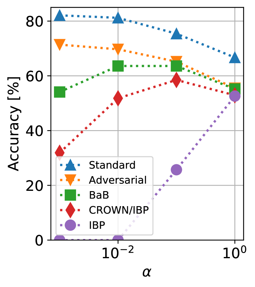
(a) CC-IBP, $\epsilon=\nicefrac{{2}}{{255}}$.

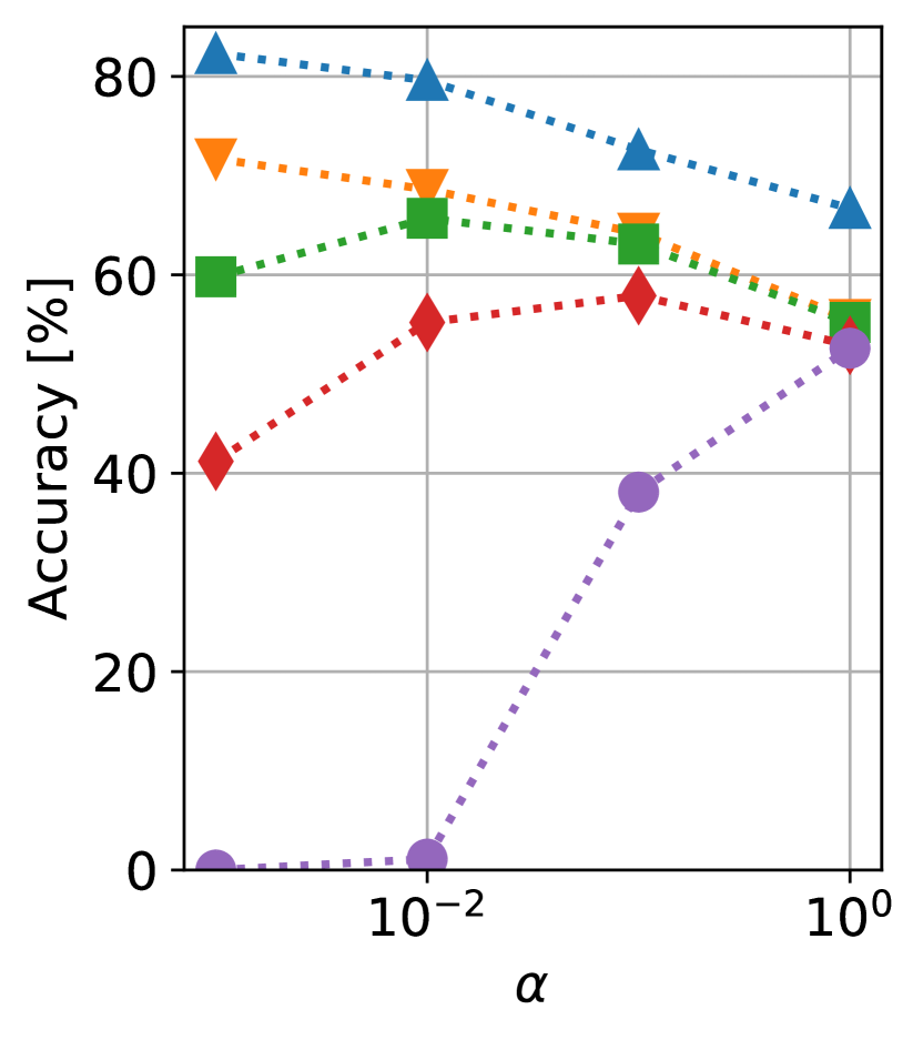
(b) MTL-IBP, $\epsilon=\nicefrac{{2}}{{255}}$.

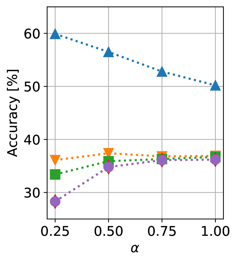
(c) CC-IBP, $\epsilon=\nicefrac{{8}}{{255}}$.

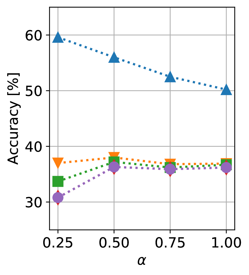
(d) MTL-IBP, $\epsilon=\nicefrac{{8}}{{255}}$.

Figure 2: Sensitivity of CC-IBP and MTL-IBP to the convex combination coefficient $\alpha$ (see $\S$3). We report standard, adversarial and verified robust accuracies (with different verifiers) under $\ell_{\infty}$ perturbations on the first $1000$ images of the CIFAR-10 test set. The legend in plot 3(a) applies to all sub-figures.

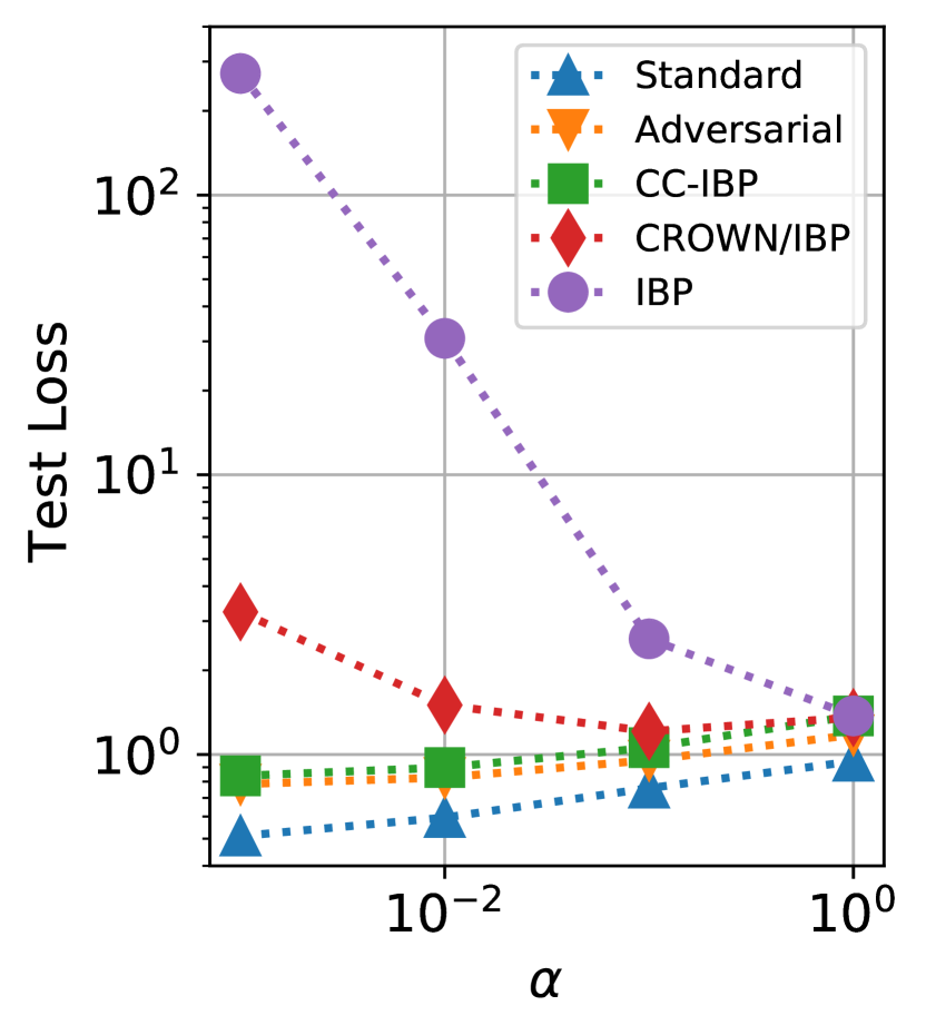
(a) CC-IBP, $\epsilon=\nicefrac{{2}}{{255}}$.

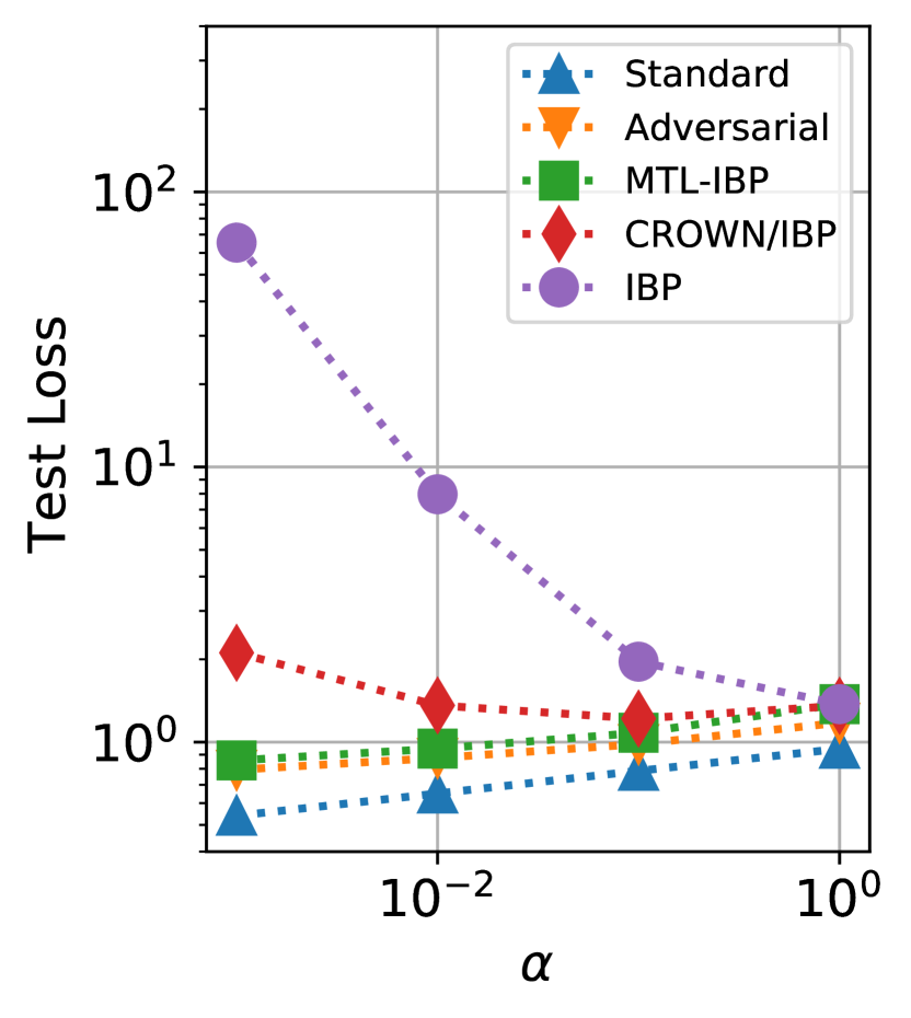
(b) MTL-IBP, $\epsilon=\nicefrac{{2}}{{255}}$.

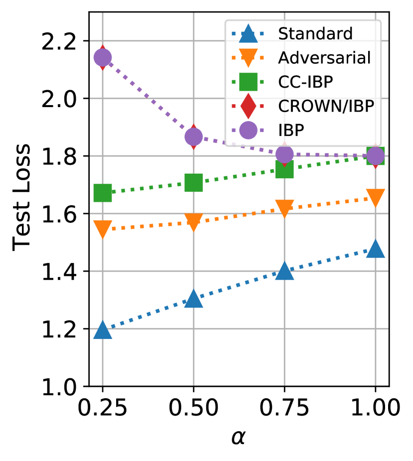
(c) CC-IBP, $\epsilon=\nicefrac{{8}}{{255}}$.

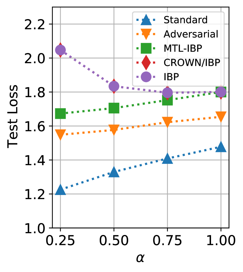
(d) MTL-IBP, $\epsilon=\nicefrac{{8}}{{255}}$.

Figure 3: Loss values (computed on the full CIFAR-10 test set) for the models from Figure 2. The CC-IBP and MTL-IBP losses (see $\S$3) are computed using the $\alpha$ value employed for training, denoted on the $x$ axis.

6 Conclusions

We showed that simple convex combinations of adversarial attacks and IBP bounds are expressive enough to cover a wide range of trade-offs between verified robustness and standard accuracy. More formally, they can be used to obtain two parametrized loss functions, named CC-IBP and MTL-IBP, that can range from the adversarial loss to the IBP loss by means of a single parameter $\alpha\in[0,1]$. We presented a comprehensive experimental evaluation of CC-IBP and MTL-IBP, showing that, in spite of their simplicity, both losses can be used to train state-of-the-art models on relevant benchmarks from the literature. On large-scale datasets (TinyImageNet and downscaled ImageNet), both CC-IBP and MTL-IBP improve upon the best literature results by a relatively large margin, incurring minimal overhead compared to standard IBP training, and often without requiring expensive verifiers based on branch-and-bound.

Appendix A Limitations and Broader Impact

Verified training algorithms attain high verified adversarial robustness at a significant cost in terms of standard model performance. For instance, state-of-the-art accuracy on CIFAR-10 has long been well above $90\%$, as opposed to roughly $80\%$ as reported in table 1. In addition, the gap between state-of-the-art empirical and verified adversarial robustness remains wide (see $\S$1), indicating either hidden vulnerabilities of adversarially-trained networks or limitations of network verifiers. Furthermore, while we demonstrated state-of-the-art performance on a suite of commonly-employed vision datasets, this does not guarantee the effectiveness of our methods beyond the tested benchmarks and, in particular, on different data domains such as natural language.

We do not foresee any immediate negative application of networks that are provably robust to adversarial perturbations. Nevertheless, the development of systems that are more robust will likely hinder any positive use of adversarial examples [1], potentially amplifying the harm caused by unethical machine learning systems.

Appendix B Expressivity of SABR

Proposition B.1.

The SABR [49] loss function $\mathcal{L}(-\underaccent{\bar}{\zb}_{\lambda}(\bm{\theta},\mathbf{x},y),y)$, defined in equation (6), is expressive according to definition 3.1.

Proof.

Recalling equation (6), $\underaccent{\bar}{\zb}_{\lambda}(\bm{\theta},\mathbf{x},y)\leq\mathbf{z}(\bm{\theta},\mathbf{x}^{\prime},y)\enskip\forall\ \mathbf{x}^{\prime}\in\mathcal{C}(\mathbf{x}_{\lambda},\lambda\epsilon)\subseteq\mathcal{C}(\mathbf{x},\epsilon)$, with $\mathbf{x}_{\lambda}:=\text{Proj}(\mathbf{x}_{\text{adv}},\mathcal{C}(\mathbf{x},\epsilon-\lambda\epsilon))$. We can hence define $\delta_{\lambda}(\bm{\theta},\mathbf{x}^{\prime},y):=\underaccent{\bar}{\zb}_{\lambda}(\bm{\theta},\mathbf{x},y)-\mathbf{z}(\bm{\theta},\mathbf{x}^{\prime},y)\leq 0$ for any $\mathbf{x}^{\prime}\in\mathcal{C}(\mathbf{x}_{\lambda},\lambda\epsilon)$. As $\mathcal{C}(\mathbf{x}_{\lambda^{\prime}},\lambda^{\prime}\epsilon)\subseteq\mathcal{C}(\mathbf{x}_{\lambda},\lambda\epsilon)$ for any $\lambda^{\prime}\leq\lambda$, $\underaccent{\bar}{\zb}_{\lambda}(\bm{\theta},\mathbf{x},y)$ will monotonically decrease with $\lambda$, and so will $\delta_{\lambda}(\bm{\theta},\mathbf{x}^{\prime},y)$. We can hence re-write the SABR loss as:

$$\mathcal{L}(-\underaccent{\bar}{\zb}_{\lambda}(\bm{\theta},\mathbf{x},y),y) =\mathcal{L}(-\left[\mathbf{z}(\bm{\theta},\mathbf{x}_{\text{adv}},y)+\left(\underaccent{\bar}{\zb}_{\lambda}(\bm{\theta},\mathbf{x},y)-\mathbf{z}(\bm{\theta},\mathbf{x}_{\text{adv}},y)\right)\right],y)$$

$$=\mathcal{L}(-\left[\mathbf{z}(\bm{\theta},\mathbf{x}_{\text{adv}},y)+\delta_{\lambda}(\bm{\theta},\mathbf{x}_{\text{adv}},y)\right],y).$$

Then, $\delta_{0}(\bm{\theta},\mathbf{x}_{\text{adv}},y)=0$, as $\mathbf{x}_{0}=\mathbf{x}_{\text{adv}}$ and hence $\underaccent{\bar}{\zb}_{0}(\bm{\theta},\mathbf{x},y)=\mathbf{z}(\bm{\theta},\mathbf{x}_{\text{adv}},y)$. Furthermore, $\underaccent{\bar}{\zb}_{1}(\bm{\theta},\mathbf{x},y)=\underaccent{\bar}{\zb}(\bm{\theta},\mathbf{x},y)$, proving the last two points of definition 3.1. The remaining requirements follow from using assumption 2.1 and the non-positivity and monotonicity of $\delta_{\lambda}(\bm{\theta},\mathbf{x}_{\text{adv}},y)$. ∎

Appendix C Loss Details for Cross-Entropy

Assuming the underlying loss function $\mathcal{L}$ to be cross-entropy, we now present an analytical form of the expressive losses presented in $\S$3.1 and $\S$3.2, along with a comparison with the loss from SABR [49].

When applied on the logit differences $\mathbf{z}(\bm{\theta},\mathbf{x},y)$ (see $\S$2.2.2), the cross-entropy can be written as $\mathcal{L}(-\mathbf{z}(\bm{\theta},\mathbf{x},y),y)=\log(1+\sum_{i\neq y}e^{-\mathbf{z}(\bm{\theta},\mathbf{x},y)[i]})$ by exploiting the properties of logarithms and $\mathbf{z}(\bm{\theta},\mathbf{x},y)[y]=0$ (see $\S$2). In fact:

$$\mathcal{L}(-\mathbf{z}(\bm{\theta},\mathbf{x},y),y) =-\log\left(\frac{e^{-\mathbf{z}(\bm{\theta},\mathbf{x},y)[y]}}{\sum_{i}e^{-\mathbf{z}(\bm{\theta},\mathbf{x},y)[i]}}\right)$$

$$=-\log\left(\frac{1}{1+\sum_{i\neq y}e^{-\mathbf{z}(\bm{\theta},\mathbf{x},y)[i]}}\right)=\log\left(1+\sum_{i\neq y}e^{-\mathbf{z}(\bm{\theta},\mathbf{x},y)[i]}\right).$$

C.1 CC-IBP

Proposition C.1.

When $\mathcal{L}(-\mathbf{z}(\bm{\theta},\mathbf{x},y),y)=\log(1+\sum_{i\neq y}e^{-\mathbf{z}(\bm{\theta},\mathbf{x},y)[i]})$, the loss $\mathcal{L}_{\alpha,\text{CC}}(\bm{\theta},\mathbf{x},y)$ from equation (7) takes the following form:

$$\mathcal{L}_{\alpha,\text{CC}}(\bm{\theta},\mathbf{x},y)=\log\left(1+\sum_{i\neq y}{\left(e^{-\mathbf{z}(\bm{\theta},\mathbf{x}_{\text{adv}},y)[i]}\right)}^{(1-\alpha)}{\left(e^{-\underaccent{\bar}{\zb}(\bm{\theta},\mathbf{x},y)[i]}\right)}^{\alpha}\right).$$

Proof.

Using the properties of exponentials:

$$\mathcal{L}_{\alpha,\text{CC}}(\bm{\theta},\mathbf{x},y) =\mathcal{L}(-\left[(1-\alpha)\ \mathbf{z}(\bm{\theta},\mathbf{x}_{\text{adv}},y)+\alpha\ \underaccent{\bar}{\zb}(\bm{\theta},\mathbf{x},y)\right],y)$$

$$=\log\left(1+\sum_{i\neq y}e^{-\left[(1-\alpha)\ \mathbf{z}(\bm{\theta},\mathbf{x}_{\text{adv}},y)+\alpha\ \underaccent{\bar}{\zb}(\bm{\theta},\mathbf{x},y)\right][i]}\right)$$

$$=\log\left(1+\sum_{i\neq y}\left(e^{-(1-\alpha)\ \mathbf{z}(\bm{\theta},\mathbf{x}_{\text{adv}},y)[i]}\right)\left(e^{-\alpha\ \underaccent{\bar}{\zb}(\bm{\theta},\mathbf{x},y)[i]}\right)\right)$$

$$=\log\left(1+\sum_{i\neq y}{\left(e^{-\mathbf{z}(\bm{\theta},\mathbf{x}_{\text{adv}},y)[i]}\right)}^{(1-\alpha)}{\left(e^{-\underaccent{\bar}{\zb}(\bm{\theta},\mathbf{x},y)[i]}\right)}^{\alpha}\right).$$

∎

C.2 MTL-IBP

Proposition C.2.

When $\mathcal{L}(-\mathbf{z}(\bm{\theta},\mathbf{x},y),y)=\log(1+\sum_{i\neq y}e^{-\mathbf{z}(\bm{\theta},\mathbf{x},y)[i]})$, the loss $\mathcal{L}_{\alpha,\text{MTL}}(\bm{\theta},\mathbf{x},y)$ from equation (8) takes the following form:

$$\mathcal{L}_{\alpha,\text{MTL}}(\bm{\theta},\mathbf{x},y)=\log\left({\left(1+\sum_{i\neq y}e^{-\mathbf{z}(\bm{\theta},\mathbf{x}_{\text{adv}},y)[i]}\right)}^{(1-\alpha)}{\left(1+\sum_{i\neq y}e^{-\underaccent{\bar}{\zb}(\bm{\theta},\mathbf{x},y)[i]}\right)}^{\alpha}\right).$$

Proof.

Using the properties of logarithms and exponentials:

$$\mathcal{L}_{\alpha,\text{MTL}}(\bm{\theta},\mathbf{x},y) =(1-\alpha)\mathcal{L}(f(\bm{\theta},\mathbf{x}_{\text{adv}}),y)+\alpha\ \mathcal{L}_{\text{ver}}(f(\bm{\theta},\mathbf{x}),y)$$

$$=(1-\alpha)\log\left(1+\sum_{i\neq y}e^{-\mathbf{z}(\bm{\theta},\mathbf{x}_{\text{adv}},y)[i]}\right)+\alpha\log\left(1+\sum_{i\neq y}e^{-\underaccent{\bar}{\zb}(\bm{\theta},\mathbf{x},y)[i]}\right)$$

$$=\log\left({\left(1+\sum_{i\neq y}e^{-\mathbf{z}(\bm{\theta},\mathbf{x}_{\text{adv}},y)[i]}\right)}^{(1-\alpha)}\right)+\log\left({\left(1+\sum_{i\neq y}e^{-\underaccent{\bar}{\zb}(\bm{\theta},\mathbf{x},y)[i]}\right)}^{\alpha}\right)$$

$$=\log\left({\left(1+\sum_{i\neq y}e^{-\mathbf{z}(\bm{\theta},\mathbf{x}_{\text{adv}},y)[i]}\right)}^{(1-\alpha)}{\left(1+\sum_{i\neq y}e^{-\underaccent{\bar}{\zb}(\bm{\theta},\mathbf{x},y)[i]}\right)}^{\alpha}\right).$$

∎

By comparing propositions C.1 and C.2, we can see that verifiability tends to play a relatively larger role on $\mathcal{L}_{\alpha,\text{MTL}}(\bm{\theta},\mathbf{x},y)$. In particular, given that $\mathbf{z}(\bm{\theta},\mathbf{x}_{\text{adv}},y)>\underaccent{\bar}{\zb}(\bm{\theta},\mathbf{x},y)$, if the network displays a large margin of empirical robustness to a given incorrect class ($\mathbf{z}(\bm{\theta},\mathbf{x}_{\text{adv}},y)[i]>>0$, with $i\neq y$), the weight of the verifiability of that class on $\mathcal{L}_{\alpha,\text{CC}}(\bm{\theta},\mathbf{x},y)$ will be greatly reduced. On the other hand, if the network has a large margin of empirical robustness to all incorrect classes ($\mathbf{z}(\bm{\theta},\mathbf{x}_{\text{adv}},y)>>\mathbf{0}$), verifiability will still have a relatively large weight on $\mathcal{L}_{\alpha,\text{MTL}}(\bm{\theta},\mathbf{x},y)$. These observations comply with proposition 3.3, which shows that $\mathcal{L}_{\alpha,\text{CC}}(\bm{\theta},\mathbf{x},y)\leq\mathcal{L}_{\alpha,\text{MTL}}(\bm{\theta},\mathbf{x},y)$, indicating that $\mathcal{L}_{\alpha,\text{MTL}}(\bm{\theta},\mathbf{x},y)$ is generally more skewed towards verifiability.

C.3 Comparison of CC-IBP with SABR

Proposition C.3.

When $\mathcal{L}(-\mathbf{z}(\bm{\theta},\mathbf{x},y),y)=\log(1+\sum_{i\neq y}e^{-\mathbf{z}(\bm{\theta},\mathbf{x},y)[i]})$, the loss $\mathcal{L}(-\underaccent{\bar}{\zb}_{\lambda}(\bm{\theta},\mathbf{x},y),y)$ from equation (6) takes the following form:

$$\mathcal{L}(-\underaccent{\bar}{\zb}_{\lambda}(\bm{\theta},\mathbf{x},y),y)=\log\left(1+\sum_{i\neq y}{\left(e^{-\mathbf{z}(\bm{\theta},\mathbf{x}_{\text{adv}},y)[i]}\right)}{\left(e^{-\delta_{\lambda}(\bm{\theta},\mathbf{x}_{\text{adv}},y)[i]}\right)}\right),$$

where $\delta_{\lambda}(\bm{\theta},\mathbf{x}_{\text{adv}},y)\leq 0$ is monotonically decreasing with $\lambda$.

Proof.

We can use $\delta_{\lambda}(\bm{\theta},\mathbf{x}^{\prime},y):=\underaccent{\bar}{\zb}_{\lambda}(\bm{\theta},\mathbf{x},y)-\mathbf{z}(\bm{\theta},\mathbf{x}^{\prime},y)\leq 0$, which is monotonically decreasing with $\lambda$ as seen in the proof of proposition B.1. Then, exploiting the properties of the exponential, we can trivially re-write the SABR loss $\mathcal{L}(-\underaccent{\bar}{\zb}_{\lambda}(\bm{\theta},\mathbf{x},y),y)$ as:

$$\mathcal{L}(-\underaccent{\bar}{\zb}_{\lambda}(\bm{\theta},\mathbf{x},y),y) =\mathcal{L}(-\left[\mathbf{z}(\bm{\theta},\mathbf{x}_{\text{adv}},y)+\delta_{\lambda}(\bm{\theta},\mathbf{x},y)\right],y)$$

$$=\log\left(1+\sum_{i\neq y}e^{-\left[\mathbf{z}(\bm{\theta},\mathbf{x}_{\text{adv}},y)+\delta_{\lambda}(\bm{\theta},\mathbf{x},y)\right][i]}\right)$$

$$=\log\left(1+\sum_{i\neq y}{\left(e^{-\mathbf{z}(\bm{\theta},\mathbf{x}_{\text{adv}},y)[i]}\right)}{\left(e^{-\delta_{\lambda}(\bm{\theta},\mathbf{x},y)[i]}\right)}\right).$$

∎

By comparing propositions C.1 and C.3, we can see that the SABR and CC-IBP losses share a similar form, and they both upper-bound the adversarial loss. The main differences are the following: (i) the adversarial term is scaled down in CC-IBP, (ii) CC-IBP computes lower bounds over the entire input region, (iii) the over-approximation term of CC-IBP uses a scaled lower bound of the logit differences, rather than its difference with the adversarial $\mathbf{z}$.

Appendix D Branch-and-Bound Framework

We now outline the details of the Branch-and-Bound (BaB) framework employed to verify the networks trained via CC-IBP and MTL-IBP (see $\S$5).

Before resorting to more expensive verifiers, we first run IBP [27] and CROWN [80] from the automatic LiRPA library [74] as an attempt to quickly verify the property. If the attempt fails, we run BaB with a timeout of $1800$ seconds per data point, possibly terminating well before the timeout (except on the MNIST experiments) when the property is deemed likely to time out. Similarly to a recent verified training work [19], we base our verifier on the publicly available OVAL framework [9, 10, 18] from VNN-COMP-2021 [4].

Lower bounds to logit differences

A crucial component of a BaB framework is the strategy employed to compute $\underaccent{\bar}{\zb}(\bm{\theta},\mathbf{x},y)$. As explained in $\S$2.2.1, the computation of the bound relies on a network over-approximation, which will generally depend on “intermediate bounds": bounds to intermediate network pre-activations. For ReLU network, the over-approximation quality will depend on the tightness of the bounds for “ambiguous" ReLUs, which cannot be replaced by a linear function ($0$ is contained in their pre-activation bounds). We first use IBP to inexpensively compute intermediate bounds for the whole network. Then, we refine the bounds associated to ambiguous ReLUs by using $5$ iterations of $\alpha$-CROWN [75] with a step size of $1$ decayed by $0.98$ at every iteration, without jointly optimizing over them so as to reduce the memory footprint. Intermediate bounds are computed only once at the root node, that is, before any branching is performed. If the property is not verified at the root, we use $\beta$-CROWN [68] as bounding algorithm for the output bounds, with a dynamic number of iterations (see [18, section 5.1.2]), and initialized from the parent BaB sub-problem. We employ a step size of $0.1$, decayed by $0.98$ at each iteration.

Adversarial attacks

Counter-examples to the properties are searched for by evaluating the network on the input points that concretize the lower bound $\underaccent{\bar}{\zb}(\bm{\theta},\mathbf{x},y)$ according to the employed network over-approximation. This is repeated on each BaB sub-problem, and also used to mark sub-problem infeasibility when $\underaccent{\bar}{\zb}(\bm{\theta},\mathbf{x},y)$ overcomes the corresponding input point evaluation. In addition, some of these points are used as initialization (along with random points in the perturbation region) for a $500$-step MI-FGSM [21] adversarial attack, which is run repeatedly for each property using a variety of randomly sampled hyper-parameter (step size value and decay, momentum) settings, and early stopped if success is deemed unlikely. In $\S$5.4 we report a network to be empirically robust if both the above procedure and a $40$-step PGD attack [44] (run before BaB) fail to find an adversarial example.

Branching

Branching is performed through activation spitting: we create branch-and-bound subproblems by splitting a ReLU into its two linear functions. In other words, given intermediate bounds on pre-activations $\mathbf{\hat{x}}_{k}\in[\hat{\mathbf{l}}_{k},\hat{\mathbf{u}}_{k}]$ for $k\in\left\llbracket 2,n-1\right\rrbracket$, if the split is performed at the $i$-th neuron of the $k$-th layer, $\hat{\mathbf{l}}_{k}[i]\geq 0$ is enforced on a sub-problem, $\hat{\mathbf{u}}_{k}[i]\leq 0$ on the other. We employ a slightly modified version of the UPB branching strategy [19, equation (7)], where the bias of the upper constraint from the Planet relaxation (ReLU convex hull, also known as triangle relaxation), $\frac{[-\hat{\mathbf{l}}_{k}]_{+}\odot[\hat{\mathbf{u}}_{k}]_{+}}{\hat{\mathbf{u}}_{k}-\hat{\mathbf{l}}_{k}}$, is replaced by the area of the entire relaxation, $[-\hat{\mathbf{l}}_{k}]_{+}\odot[\hat{\mathbf{u}}_{k}]_{+}$. Intuitively, the area of the over-approximation should better represent the weight of an ambiguous neuron in the overall neural network relaxation than the distance of the upper constraint from the origin. In practice, we found the impact on BaB performance to be negligible. In particular, we tested our variant against the original UPB, leaving the remaining BaB setup unchanged, on the CC-IBP trained network for MNIST with $\epsilon=0.1$ from table 1: they both resulted in $98.43\%$ verified robust accuracy.

Appendix E Experimental Details

We present additional details pertaining to the experiments from $\S$5 and appendix F. In particular, we outline dataset and training details, hyper-parameters, computational setup and the employed network architecture.

E.1 Datasets

MNIST [40] is a $10$-class (each class being a handwritten digit) classification dataset consisting of $28\times 28$ greyscale images, with 60,000 training and 10,000 test points. CIFAR-10 [36] consists of $32\times 32$ RGB images in 10 different classes (associated to subjects such as airplanes, cars, etc.), with 50,000 training and 10,000 test points. TinyImageNet [39] is a miniature version of the ImageNet dataset, restricted to 200 classes of $64\times 64$ RGB images, with 100,000 training and 10,000 validation images. The employed downscaled ImageNet [12] is a 1000-class dataset of $64\times 64$ RGB images, with 1,281,167 training and 50,000 validation images. Similarly to previous work [74, 54, 49], we normalize all datasets and use random horizontal flips and random cropping as data augmentation on CIFAR-10, TinyImageNet and downscaled ImageNet. Complying with common experimental practice [27, 74, 54, 49], we train on the entire training sets, and evaluate MNIST and CIFAR-10 on their test sets, ImageNet and TinyImageNet on their validation sets.

E.2 Network Architecture, Training Schedule and Hyper-parameters

We outline the practical details of our training procedure.

Table 4: Details of the CNN7 architecture.

CNN7 Convolutional: $64$ filters of size $3\times 3$, stride $1$, padding $1$ BatchNorm layer ReLU layer Convolutional layer: $64$ filters of size $3\times 3$, stride $1$, padding $1$ BatchNorm layer ReLU layer Convolutional layer: $128$ filters of size $3\times 3$, stride $2$, padding $1$ BatchNorm layer ReLU layer Convolutional layer: $128$ filters of size $3\times 3$, stride $1$, padding $1$ BatchNorm layer ReLU layer Convolutional layer: $128$ filters of size $3\times 3$, stride $1$, padding $1$ BatchNorm layer ReLU layer Linear layer: $512$ hidden units BatchNorm layer ReLU layer Linear layer: as many hidden units as the number of classes

Network Architecture

Independently of the dataset, all our experiments employ a 7-layer architecture that enjoys widespread usage in the verified training literature [27, 81, 54, 49, 45]. In particular, mirroring recent work [49, 45], we employ a version modified by Shi et al. [54] to employ BatchNorm [32] after every layer. Complying with Shi et al. [54], at training time we compute IBP bounds to BatchNorm layers using the batch statistics from unperturbed data. The statistics used at evaluation time are instead computed including both the original data and the attacks used during training. The details of the architecture, often named CNN7 in the literature, are presented in table 4.

Table 5: Hyper-parameter configurations for the networks trained via CC-IBP and MTL-IBP from table 1.

Dataset $\epsilon$ Method $\alpha$ $\ell_{1}$ Attack $\eta$ Attack steps Total epochs Warm-up + Ramp-up LR decay epochs MNIST $0.1$ CC-IBP $1\times 10^{-1}$ $2\times 10^{-6}$ $10.0\epsilon$ 1 70 0+20 50,60 MTL-IBP $1\times 10^{-2}$ $1\times 10^{-5}$ $10.0\epsilon$ 1 70 0+20 50,60 $0.3$ CC-IBP $3\times 10^{-1}$ $3\times 10^{-6}$ $10.0\epsilon$ 1 70 0+20 50,60 MTL-IBP $8\times 10^{-2}$ $1\times 10^{-6}$ $10.0\epsilon$ 1 70 0+20 50,60 CIFAR-10 $\frac{2}{255}$ CC-IBP $1\times 10^{-2}$ $3\times 10^{-6}$ $0.25\epsilon$ 8 160 1+80 120,140 MTL-IBP $4\times 10^{-3}$ $3\times 10^{-6}$ $0.25\epsilon$ 8 160 1+80 120,140 $\frac{8}{255}$ CC-IBP $5\times 10^{-1}$ 0 $10.0\epsilon$ 1 260 1+80 180,220 MTL-IBP $5\times 10^{-1}$ $1\times 10^{-7}$ $10.0\epsilon$ 1 260 1+80 180,220 TinyImageNet $\frac{1}{255}$ CC-IBP $2\times 10^{-1}$ $2\times 10^{-5}$ $10.0\epsilon$ 1 160 1+80 120,140 MTL-IBP $2\times 10^{-1}$ $2\times 10^{-5}$ $10.0\epsilon$ 1 160 1+80 120,140 ImageNet64 $\frac{1}{255}$ CC-IBP $5\times 10^{-2}$ $1\times 10^{-5}$ $10.0\epsilon$ 1 80 1+20 60,70 MTL-IBP $5\times 10^{-2}$ $1\times 10^{-5}$ $10.0\epsilon$ 1 80 1+20 60,70

Train-Time Perturbation Radius

We train using the target perturbation radius (denoted by $\epsilon$ as elsewhere in this work) for all benchmarks except on MNIST and CIFAR-10 when $\epsilon=\nicefrac{{2}}{{255}}$. On MNIST, complying with Shi et al. [54], we use $\epsilon_{\text{train}}=0.2$ for $\epsilon=0.1$ and $\epsilon_{\text{train}}=0.4$ for $\epsilon=0.3$. On CIFAR-10 with $\epsilon=\nicefrac{{2}}{{255}}$, in order to improve performance, SABR [49] “shrinks" the magnitude of the computed IBP bounds by multiplying intermediate bounds by a constant $c=0.8$ before each ReLU (for instance, following our notation in $\S$2.2.1 $[\hat{\mathbf{u}}_{k-1}]_{+}$ would be replaced by $0.8[\hat{\mathbf{u}}_{k-1}]_{+}$). As a result, the prominence of the attack in the employed loss function is increased. In other to achieve a similar effect, we employ the original perturbation radius to compute the lower bounds $\underaccent{\bar}{\zb}(\bm{\theta},\mathbf{x},y)$ and use a larger perturbation radius to compute $\mathbf{x}_{\text{adv}}$ for both CC-IBP and MTL-IBP. Specifically, we use $\epsilon_{\text{train}}=4.2$, the radius employed by IBP-R [19] to perform the attack and to compute the algorithm’s regularization terms.

Training Schedule

Following Shi et al. [54], training proceeds as follows: the network is initialized according to the method presented by Shi et al. [54]. Training starts with the standard cross-entropy loss during warm-up. Then, the perturbation radius is gradually increased to the target value $\epsilon_{\text{train}}$ (using the same schedule as Shi et al. [54]) for a fixed number of epochs during the ramp-up phase. During warmp-up and ramp-up, the regularization introduced by Shi et al. [54] is added to the objective. Finally, towards the end of training, and after ramp-up has ended, the learning rate is decayed twice. In line with previous work [72, 19, 49, 45], we employ $\ell_{1}$ regularization throughout training.

Hyper-parameters

The hyper-parameter configurations used in table 1 are presented in table 5. The training schedules for MNIST and CIFAR-10 with $\epsilon=\nicefrac{{2}}{{255}}$ follow the hyper-parameters from Shi et al. [54]. Similarly to Müller et al. [49], we increase the number of epochs after ramp-up for CIFAR-10 with $\epsilon=\nicefrac{{8}}{{255}}$: we use $260$ epochs in total. On TinyImageNet, we employ the same configuration as CIFAR-10 with $\epsilon=\nicefrac{{2}}{{255}}$, and ImageNet64 relies on the TinyImageNet schedule from Shi et al. [54], who did not benchmark on it. Following previous work [54, 49], we use a batch size of $256$ for MNIST, and of $128$ everywhere else. As Shi et al. [54], Müller et al. [49], we use a learning rate of $5\times 10^{-5}$ for all experiments, decayed twice by a factor of $0.2$, and use gradient clipping with threshold equal to $10$. Coefficients for the regularization introduced by Shi et al. [54] are set to the values suggested in the author’s official codebase: $\lambda=0.5$ on MNIST and CIFAR-10, $\lambda=0.2$ for TinyImageNet. On ImageNet64, which was not included in their experiments, we use $\lambda=0.2$ as for TinyImageNet given the dataset similarities. Single-step attacks were forced to lay on the boundary of the perturbation region (see appendix F.2), while we complied with previous work for the $8$-step PGD attack [5, 19]. As Shi et al. [54], we clip target epsilon values to the fifth decimal digit. The main object of our tuning were the $\alpha$ coefficients from the CC-IBP and MTL-IBP losses (see $\S$3) and the $\ell_{1}$ regularization coefficient: for both, we first selected an order of magnitude, then the significand via manual search. In order to reduce training and verification overheads across benchmarks, we comply with the seemingly standard practice in the area [27, 81, 54, 49] and directly tune on the evaluation sets. We do not perform early stopping. Unless otherwise stated, all the ablation studies re-use the hyper-parameter configurations from table 5. In particular, the ablation from $\S$5.4 use the single-step attack for CIFAR-10 with $\epsilon=\nicefrac{{2}}{{255}}$. Furthermore, the ablation from $\S$5.2 uses $\alpha=5\times 10^{-2}$ for CC-IBP and $\alpha=1\times 10^{-2}$ for MTL-IBP in order to ease verification.

E.3 Computational Setup

All the experiments were run on $3$ different machines running Ubuntu: two with a $12$-core Intel i7-6850K CPU, and one with a $20$-core Intel i9-7900X CPU. While each experiment (both for training and post-training verification) was run on a single GPU at a time, we used a total of $8$ GPUs of the following models: Nvidia Titan V, Nvidia Titan XP, and Nvidia Titan XP. The reported timings for the training experiments (table 1) were run on a Nvidia Titan V GPU and using the $20$-core Intel i9-7900X CPU.

E.4 Software Acknowledgments

Our training code is mostly built on the publicly available training pipeline by Shi et al. [54], which was released under a 3-Clause BSD license. We further rely on the automatic LiRPA library [74], also released under a 3-Clause BSD license, and on the OVAL complete verification framework [9, 18], released under a MIT license. MNIST and CIFAR-10 are taken from torchvision.datasets [51]; we downloaded TinyImageNet from the Stanford CS231n course website (http://cs231n.stanford.edu/TinyImageNet-200.zip), and downscaled ImageNet from the ImageNet website (https://www.image-net.org/download.php).

Appendix F Additional Experimental Results

We now present experimental results omitted from $\S$5.

F.1 Experimental Variability

In order to provide an indication of experimental variability for the results from $\S$ 5, we repeat a small subset of our experiments from table 1, those on CIFAR-10 with $\epsilon=\nicefrac{{8}}{{255}}$, a further three times. Table 6 reports the mean, maximal and minimal values in addition to the sample standard deviation for both the standard and verified robust accuracies. In all cases, the experimental variability is relatively small.

Table 6: Experimental variability for the performance of CC-IBP and MTL-IBP for $\ell_{\infty}$ norm perturbations of radius $\epsilon=\nicefrac{{8}}{{255}}$ on the CIFAR-10 test set.

Method Standard accuracy [%] Verified robust accuracy [%] Mean Std. Max Min Mean Std. Max Min CC-IBP $54.04$ $00.23$ $54.23$ $53.71$ $35.06$ $00.29$ $35.34$ $34.73$ MTL-IBP $53.77$ $0.40$ $54.18$ $53.35$ $35.25$ $0.18$ $35.44$ $35.05$

F.2 Ablation: Adversarial Attack Step Size

Table 7: Effect of the attack step size $\eta$ on the performance of CC-IBP and MTL-IBP under $\ell_{\infty}$ norm perturbations on the CIFAR-10 test set.

$\epsilon$ Method Attack $\eta$ Accuracy [%] Std. Ver. rob. $\frac{2}{255}$ CC-IBP $10.0\ \epsilon$ $80.22$ $62.94$ CC-IBP $1.25\ \epsilon$ $80.94$ $62.50$ MTL-IBP $10.0\ \epsilon$ $79.70$ $62.67$ MTL-IBP $1.25\ \epsilon$ $80.43$ $62.29$ $\frac{8}{255}$ CC-IBP $10.0\ \epsilon$ $53.71$ $35.27$ CC-IBP $1.25\ \epsilon$ $54.75$ $34.77$ MTL-IBP $10.0\ \epsilon$ $53.35$ $35.44$ MTL-IBP $1.25\ \epsilon$ $54.30$ $35.38$

Section 5.2 investigates the influence of the type of attack used to compute $\mathbf{z}(\bm{\theta},\mathbf{x}_{\text{adv}},y)$ at training time on the performance of CC-IBP and MTL-IBP. We now perform a complementary ablation by keeping the attack fixed to randomly-initialized FGSM [26, 71] and changing the attack step size $\eta$. The results from $\S$5 (except for the PGD entry in table 2) employ a step size $\eta=10.0\ \epsilon$ (any value larger than $2.0\ \epsilon$ yields the same effect) in order to force the attack on the boundary of the perturbation region. Specifically, we report the performance for $\eta=1.25\ \epsilon$, which was shown by Wong et al. [71] to prevent catastrophic overfitting. Table 7 does not display significant performance differences depending on the step size, highlighting the lack of catastrophic overfitting. We speculate that this is linked to the regularizing effect of the IBP bounds employed within CC-IBP and MTL-IBP. On all considered settings, the use of larger $\eta$ results in larger standard accuracy, and a decreased verified robust accuracy.

References

- Albert et al. [2021] K. Albert, M. Delano, B. Kulynych, and R. S. S. Kumar. Adversarial for good? how the adversarial ml community’s values impede socially beneficial uses of attacks. In ICML 2021 workshop on A Blessing in Disguise: The Prospects and Perils of Adversarial Machine Learning, 2021.
- Anderson et al. [2020] R. Anderson, J. Huchette, W. Ma, C. Tjandraatmadja, and J. P. Vielma. Strong mixed-integer programming formulations for trained neural networks. Mathematical Programming, 2020.
- Athalye et al. [2018] A. Athalye, N. Carlini, and D. A. Wagner. Obfuscated gradients give a false sense of security: circumventing defenses to adversarial examples. In International Conference on Machine Learning, 2018.
- Bak et al. [2021] S. Bak, C. Liu, and T. Johnson. The second international verification of neural networks competition (VNN-COMP 2021): Summary and results. arXiv preprint arXiv:2109.00498, 2021.
- Balunovic and Vechev [2020] M. Balunovic and M. Vechev. Adversarial training and provable defenses: Bridging the gap. International Conference on Learning Representations, 2020.
- Botoeva et al. [2020] E. Botoeva, P. Kouvaros, J. Kronqvist, A. Lomuscio, and R. Misener. Efficient verification of neural networks via dependency analysis. In AAAI Conference on Artificial Intelligence, 2020.
- Boyd and Vandenberghe [2004] S. Boyd and L. Vandenberghe. Convex optimization. Cambridge university press, 2004.
- Bunel et al. [2018] R. Bunel, I. Turkaslan, P. H. Torr, P. Kohli, and M. P. Kumar. A unified view of piecewise linear neural network verification. Neural Information Processing Systems, 2018.
- Bunel et al. [2020a] R. Bunel, A. De Palma, A. Desmaison, K. Dvijotham, P. Kohli, P. H. Torr, and M. P. Kumar. Lagrangian decomposition for neural network verification. Conference on Uncertainty in Artificial Intelligence, 2020a.
- Bunel et al. [2020b] R. Bunel, J. Lu, I. Turkaslan, P. Kohli, P. Torr, and M. P. Kumar. Branch and bound for piecewise linear neural network verification. Journal of Machine Learning Research, 21(2020), 2020b.
- Caruana [1997] R. Caruana. Multitask learning. Machine Learning, 28(1):41–75, 1997.
- Chrabaszcz et al. [2017] P. Chrabaszcz, I. Loshchilov, and F. Hutter. A downsampled variant of ImageNet as an alternative to the CIFAR datasets. arXiv:1707.08819, 2017.
- Cohen et al. [2019] J. Cohen, E. Rosenfeld, and Z. Kolter. Certified adversarial robustness via randomized smoothing. In International Conference on Machine Learning, 2019.
- Croce and Hein [2020] F. Croce and M. Hein. Reliable evaluation of adversarial robustness with an ensemble of diverse parameter-free attacks. In International Conference on Machine Learning, 2020.
- Dathathri et al. [2020] S. Dathathri, K. D. Dvijotham, A. Kurakin, A. Raghunathan, J. Uesato, R. Bunel, S. Shankar, J. Steinhardt, I. Goodfellow, P. Liang, and P. Kohli. Enabling certification of verification-agnostic networks via memory-efficient semidefinite programming. In Neural Information Processing Systems, 2020.
- De Palma et al. [2021a] A. De Palma, H. S. Behl, R. Bunel, P. H. S. Torr, and M. P. Kumar. Scaling the convex barrier with active sets. International Conference on Learning Representations, 2021a.
- De Palma et al. [2021b] A. De Palma, H. S. Behl, R. Bunel, P. H. S. Torr, and M. P. Kumar. Scaling the convex barrier with sparse dual algorithms. arXiv preprint arXiv:2101.05844, 2021b.
- De Palma et al. [2021c] A. De Palma, R. Bunel, A. Desmaison, K. Dvijotham, P. Kohli, P. H. Torr, and M. P. Kumar. Improved branch and bound for neural network verification via Lagrangian decomposition. arXiv preprint arXiv:2104.06718, 2021c.
- De Palma et al. [2022] A. De Palma, R. Bunel, K. Dvijotham, M. P. Kumar, and R. Stanforth. IBP regularization for verified adversarial robustness via branch-and-bound. In ICML 2022 Workshop on Formal Verification of Machine Learning, 2022.
- Deng et al. [2009] J. Deng, W. Dong, R. Socher, L.-J. Li, K. Li, and L. Fei-Fei. Imagenet: A large-scale hierarchical image database. In Proceedings of the IEEE conference on computer vision and pattern recognition, 2009.
- Dong et al. [2018] Y. Dong, F. Liao, T. Pang, H. Su, J. Zhu, X. Hu, and J. Li. Boosting adversarial attacks with momentum. In Proceedings of the IEEE conference on computer vision and pattern recognition, pages 9185–9193, 2018.
- Ehlers [2017] R. Ehlers. Formal verification of piece-wise linear feed-forward neural networks. Automated Technology for Verification and Analysis, 2017.
- Fan and Li [2021] J. Fan and W. Li. Adversarial training and provable robustness: A tale of two objectives. In AAAI Conference on Artificial Intelligence, 2021.
- Fawzi et al. [2022] A. Fawzi, M. Balog, A. Huang, T. Hubert, B. Romera-Paredes, M. Barekatain, A. Novikov, F. J. R Ruiz, J. Schrittwieser, G. Swirszcz, et al. Discovering faster matrix multiplication algorithms with reinforcement learning. Nature, 2022.
- Ferrari et al. [2022] C. Ferrari, M. N. Mueller, N. Jovanović, and M. Vechev. Complete verification via multi-neuron relaxation guided branch-and-bound. International Conference on Learning Representations, 2022.
- Goodfellow et al. [2015] I. J. Goodfellow, J. Shlens, and C. Szegedy. Explaining and harnessing adversarial examples. International Conference on Learning Representations, 2015.
- Gowal et al. [2018] S. Gowal, K. Dvijotham, R. Stanforth, R. Bunel, C. Qin, J. Uesato, T. Mann, and P. Kohli. On the effectiveness of interval bound propagation for training verifiably robust models. Workshop on Security in Machine Learning, NeurIPS, 2018.
- Henriksen and Lomuscio [2020] P. Henriksen and A. Lomuscio. Efficient neural network verification via adaptive refinement and adversarial search. In European Conference on Artificial Intelligence, 2020.
- Henriksen and Lomuscio [2021] P. Henriksen and A. Lomuscio. Deepsplit: An efficient splitting method for neural network verification via indirect effect analysis. In Proceedings of the 30th International Joint Conference on Artificial Intelligence (IJCAI21), 2021.
- Hickey et al. [2001] T. Hickey, Q. Ju, and M. H. Van Emden. Interval arithmetic: From principles to implementation. Journal of the ACM (JACM), 2001.
- Huang et al. [2021] Y. Huang, H. Zhang, Y. Shi, J. Z. Kolter, and A. Anandkumar. Training certifiably robust neural networks with efficient local lipschitz bounds. In Neural Information Processing Systems, 2021.
- Ioffe and Szegedy [2015] S. Ioffe and C. Szegedy. Batch normalization: Accelerating deep network training by reducing internal covariate shift. In International Conference on Machine Learning, 2015.
- Jovanović et al. [2022] N. Jovanović, M. Balunović, M. Baader, and M. T. Vechev. On the paradox of certified training. In Transactions on Machine Learning Research, 2022.
- Jumper et al. [2021] J. Jumper, R. Evans, A. Pritzel, T. Green, M. Figurnov, O. Ronneberger, K. Tunyasuvunakool, R. Bates, A. Žídek, A. Potapenko, et al. Highly accurate protein structure prediction with alphafold. Nature, 2021.
- Katz et al. [2017] G. Katz, C. Barrett, D. Dill, K. Julian, and M. Kochenderfer. Reluplex: An efficient SMT solver for verifying deep neural networks. Computer Aided Verification, 2017.
- Krizhevsky and Hinton [2009] A. Krizhevsky and G. Hinton. Learning multiple layers of features from tiny images. Master’s thesis, Department of Computer Science, University of Toronto, 2009.
- Kurin et al. [2022] V. Kurin, A. De Palma, I. Kostrikov, S. Whiteson, and M. P. Kumar. In defense of the unitary scalarization for deep multi-task learning. In Neural Information Processing Systems, 2022.
- Lan et al. [2022] J. Lan, Y. Zheng, and A. Lomuscio. Tight neural network verification via semidefinite relaxations and linear reformulations. In AAAI Conference on Artificial Intelligence, 2022.
- Le and Yang [2015] Y. Le and X. S. Yang. Tiny imagenet visual recognition challenge. 2015.
- LeCun et al. [2010] Y. LeCun, C. Cortes, and C. Burges. Mnist handwritten digit database. ATT Labs [Online]. Available: http://yann.lecun.com/exdb/mnist, 2, 2010.
- Lee et al. [2021] S. Lee, W. Lee, J. Park, and J. Lee. Towards better understanding of training certifiably robust models against adversarial examples. In Neural Information Processing Systems, 2021.
- Leino et al. [2021] K. Leino, Z. Wang, and M. Fredrikson. Globally-robust neural networks. In International Conference on Machine Learning, 2021.
- Lomuscio and Maganti [2017] A. Lomuscio and L. Maganti. An approach to reachability analysis for feed-forward ReLU neural networks. arXiv:1706.07351, 2017.
- Madry et al. [2018] A. Madry, A. Makelov, L. Schmidt, D. Tsipras, and A. Vladu. Towards deep learning models resistant to adversarial attacks. International Conference on Learning Representations, 2018.
- Mao et al. [2023] Y. Mao, M. N. Müller, M. Fischer, and M. Vechev. TAPS: Connecting certified and adversarial training. arXiv:2305.04574, 2023.
- Mirman et al. [2018] M. Mirman, T. Gehr, and M. Vechev. Differentiable abstract interpretation for provably robust neural networks. International Conference on Machine Learning, 2018.
- Müller et al. [2022] M. N. Müller, C. Brix, S. Bak, C. Liu, and T. Johnson. The second international verification of neural networks competition (VNN-COMP 2021): Summary and results. arXiv preprint arXiv:2212.10376, 2022.
- Müller et al. [2022] M. N. Müller, G. Makarchuk, G. Singh, M. Püschel, and M. Vechev. PRIMA: General and precise neural network certification via scalable convex hull approximations. Proceedings of the ACM on Programming Languages, 2022.
- Müller et al. [2023] M. N. Müller, F. Eckert, M. Fischer, and M. Vechev. Certified training: Small boxes are all you need. In International Conference on Learning Representations, 2023.
- OpenAI [2023] OpenAI. GPT-4 technical report. arXiv preprint arXiv:2303.08774, 2023.
- Paszke et al. [2019] A. Paszke, S. Gross, F. Massa, A. Lerer, J. Bradbury, G. Chanan, T. Killeen, Z. Lin, N. Gimelshein, L. Antiga, A. Desmaison, A. Kopf, E. Yang, Z. DeVito, M. Raison, A. Tejani, S. Chilamkurthy, B. Steiner, L. Fang, J. Bai, and S. Chintala. Pytorch: An imperative style, high-performance deep learning library. Neural Information Processing Systems, 2019.
- Raghunathan et al. [2018] A. Raghunathan, J. Steinhardt, and P. S. Liang. Semidefinite relaxations for certifying robustness to adversarial examples. Neural Information Processing Systems, 2018.
- Salman et al. [2019] H. Salman, G. Yang, J. Li, P. Zhang, H. Zhang, I. Razenshteyn, and S. Bubeck. Provably robust deep learning via adversarially trained smoothed classifiers. In Neural Information Processing Systems, 2019.
- Shi et al. [2021] Z. Shi, Y. Wang, H. Zhang, J. Yi, and C.-J. Hsieh. Fast certified robust training with short warmup. In Neural Information Processing Systems, 2021.
- Simonyan and Zisserman [2015] K. Simonyan and A. Zisserman. Very deep convolutional networks for large-scale image recognition. In International Conference on Learning Representations, 2015.
- Singh et al. [2018] G. Singh, T. Gehr, M. Mirman, M. Püschel, and M. Vechev. Fast and effective robustness certification. Neural Information Processing Systems, 2018.
- Singh et al. [2019a] G. Singh, R. Ganvir, M. Püschel, and M. Vechev. Beyond the single neuron convex barrier for neural network certification. Neural Information Processing Systems, 2019a.
- Singh et al. [2019b] G. Singh, T. Gehr, M. Püschel, and M. Vechev. An abstract domain for certifying neural networks. Proceedings of the ACM on Programming Languages, 2019b.
- Singh et al. [2023] N. D. Singh, F. Croce, and M. Hein. Revisiting adversarial training for ImageNet: Architectures, training and generalization across threat models. arXiv:2303.01870, 2023.
- Singla and Feizi [2021] S. Singla and S. Feizi. Skew orthogonal convolutions. In International Conference on Machine Learning, 2021.
- Singla and Feizi [2022] S. Singla and S. Feizi. Improved techniques for deterministic l2 robustness. In Neural Information Processing Systems, 2022.
- Singla et al. [2022] S. Singla, S. Singla, and S. Feizi. Improved deterministic l2 robustness on CIFAR-10 and CIFAR-100. In International Conference on Learning Representations, 2022.
- Sunaga [1958] T. Sunaga. Theory of an interval algebra and its application to numerical analysis. RAAG Memoirs, 1958.
- Szegedy et al. [2014] C. Szegedy, W. Zaremba, I. Sutskever, J. Bruna, D. Erhan, I. Goodfellow, and R. Fergus. Intriguing properties of neural networks. International Conference on Learning Representations, 2014.
- Tjandraatmadja et al. [2020] C. Tjandraatmadja, R. Anderson, J. Huchette, W. Ma, K. Patel, and J. P. Vielma. The convex relaxation barrier, revisited: Tightened single-neuron relaxations for neural network verification. Neural Information Processing Systems, 2020.
- Trockman and Kolter [2021] A. Trockman and J. Z. Kolter. Orthogonalizing convolutional layers with the cayley transform. In International Conference on Learning Representations, 2021.
- Uesato et al. [2018] J. Uesato, B. O’Donoghue, A. v. d. Oord, and P. Kohli. Adversarial risk and the dangers of evaluating against weak attacks. In International Conference on Machine Learning, 2018.
- Wang et al. [2021] S. Wang, H. Zhang, K. Xu, X. Lin, S. Jana, C.-J. Hsieh, and J. Z. Kolter. Beta-CROWN: Efficient bound propagation with per-neuron split constraints for complete and incomplete neural network verification. Neural Information Processing Systems, 2021.
- Wong and Kolter [2018] E. Wong and Z. Kolter. Provable defenses against adversarial examples via the convex outer adversarial polytope. International Conference on Machine Learning, 2018.
- Wong et al. [2018] E. Wong, F. Schmidt, J. H. Metzen, and J. Z. Kolter. Scaling provable adversarial defenses. Neural Information Processing Systems, 2018.
- Wong et al. [2020] E. Wong, L. Rice, and J. Z. Kolter. Fast is better than free: Revisiting adversarial training. In International Conference on Learning Representations, 2020.
- Xiao et al. [2019] K. Xiao, V. Tjeng, N. M. Shafiullah, and A. Madry. Training for faster adversarial robustness verification via inducing relu stability. International Conference on Learning Representations, 2019.
- Xin et al. [2022] D. Xin, B. Ghorbani, A. Garg, O. Firat, and J. Gilmer. Do current multi-task optimization methods in deep learning even help? In Neural Information Processing Systems, 2022.
- Xu et al. [2020] K. Xu, Z. Shi, H. Zhang, Y. Wang, K.-W. Chang, M. Huang, B. Kailkhura, X. Lin, and C.-J. Hsieh. Automatic perturbation analysis for scalable certified robustness and beyond. In Neural Information Processing Systems, 2020.
- Xu et al. [2021] K. Xu, H. Zhang, S. Wang, Y. Wang, S. Jana, X. Lin, and C.-J. Hsieh. Fast and complete: Enabling complete neural network verification with rapid and massively parallel incomplete verifiers. In International Conference on Learning Representations, 2021.
- Xu et al. [2022] X. Xu, L. Li, and B. Li. Lot: Layer-wise orthogonal training on improving l2 certified robustness. In Neural Information Processing Systems, 2022.
- Zhang et al. [2021] B. Zhang, T. Cai, Z. Lu, D. He, and L. Wang. Towards certifying l-infinity robustness using neural networks with l-inf-dist neurons. In International Conference on Machine Learning, 2021.
- Zhang et al. [2022a] B. Zhang, D. Jiang, D. He, and L. Wang. Boosting the certified robustness of l-infinity distance nets. In International Conference on Learning Representations, 2022a.
- Zhang et al. [2022b] B. Zhang, D. Jiang, D. He, and L. Wang. Rethinking lipschitz neural networks and certified robustness: A boolean function perspective. In Neural Information Processing Systems, 2022b.
- Zhang et al. [2018] H. Zhang, T.-W. Weng, P.-Y. Chen, C.-J. Hsieh, and L. Daniel. Efficient neural network robustness certification with general activation functions. Neural Information Processing Systems, 2018.
- Zhang et al. [2020] H. Zhang, H. Chen, C. Xiao, S. Gowal, R. Stanforth, B. Li, D. Boning, and C.-J. Hsieh. Towards stable and efficient training of verifiably robust neural networks. International Conference on Learning Representations, 2020.
- Zhang et al. [2022c] H. Zhang, S. Wang, K. Xu, L. Li, B. Li, S. Jana, C.-J. Hsieh, and J. Z. Kolter. General cutting planes for bound-propagation-based neural network verification. Neural Information Processing Systems, 2022c.