On Structural Expressive Power of Graph Transformers

Abstract.

Graph Transformer has recently received wide attention in the research community with its outstanding performance, yet its structural expressive power has not been well analyzed. Inspired by the connections between Weisfeiler-Lehman (WL) graph isomorphism test and graph neural network (GNN), we introduce SEG-WL test (Structural Encoding enhanced Global Weisfeiler-Lehman test), a generalized graph isomorphism test algorithm as a powerful theoretical tool for exploring the structural discriminative power of graph Transformers. We theoretically prove that the SEG-WL test is an expressivity upper bound on a wide range of graph Transformers, and the representational power of SEG-WL test can be approximated by a simple Transformer network arbitrarily under certain conditions. With the SEG-WL test, we show how graph Transformers’ expressive power is determined by the design of structural encodings, and present conditions that make the expressivity of graph Transformers beyond WL test and GNNs. Moreover, motivated by the popular shortest path distance encoding, we follow the theory-oriented principles and develop a provably stronger structural encoding method, Shortest Path Induced Subgraph (SPIS) encoding. Our theoretical findings provide a novel and practical paradigm for investigating the expressive power of graph Transformers, and extensive synthetic and real-world experiments empirically verify the strengths of our proposed methods.

1. Introduction

In the last decade, graph neural network (GNN) (Kipf and Welling, 2016; Veličković et al., 2017) has become the prevalent neural architecture for deep learning on graph data. Following the message-passing scheme, GNNs learn the vector representation of node $v$ by iteratively aggregating and transforming features of its neighborhood nodes. Recent studies (Xu et al., 2018) have proved that Weisfeiler-Lehman (WL) graph isomorphism test can measure the theoretical expressive power of message-passing GNNs in distinguishing graph structures (Weisfeiler and Leman, 1968).

While in the last few years, the Transformer architecture (Vaswani et al., 2017) has achieved broad success in various machine learning tasks. On graph representation learning, though with higher complexity than GNNs, recent works (Ying et al., 2021; Kreuzer et al., 2021) have proved that graph Transformers can successfully model large-scale graph data and deliver state-of-the-art performance on real-world benchmarks. However, despite advances in empirical benchmark results, the theoretical expressive power of graph Transformers has not been deeply explored. Compared with GNN’s message-passing strategy, which only includes neighborhood aggregation, most graph Transformers represent nodes by considering all pair-wise interactions in the input graph, meaning that every node has a global receptive field at each layer. Besides, since vanilla self-attention is ignorant of node ordering, like positional encodings in language models, graph Transformers must design various structural encodings as a soft inductive bias to leverage graph structural information. Therefore, previous methods like WL test can no longer be used to analyze the expressivity of graph Transformers, considering the substantial differences between two model architectures. The natural questions arise: How to characterize the structural expressive power of graph Transformers? How to build expressive graph Transformers that can outperform the WL test and GNNs?

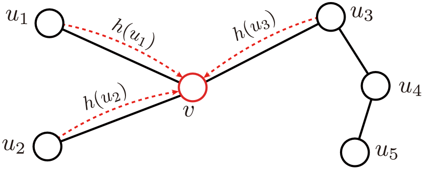
(a) WL Test

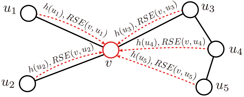
(b) SEG-WL Test

Figure 1. An illustration of the node label update strategies of WL test and SEG-WL test.

Our key to answering the questions above is SEG-WL test (Structural Encoding enhanced Global Weisfeiler-Lehman test), a generalized graph isomorphism test algorithm designed to characterize the expressivity of graph Transformer, as illustrated in Figure 1. Specifically, SEG-WL test represents a family of graph isomorphism test algorithms whose label update strategy is shaped by predefined structural encodings. For every input graph, SEG-WL test first inserts absolute structural encodings to the initial node labels. Then during each iteration, unlike WL test which updates the node label of $v$ by hashing the multiset of its neighborhood node labels $\{\mskip-5.0mu\{h(u):u\in{\mathcal{N}}(v)\}\mskip-5.0mu\}$, SEG-WL test globally hashes $\{\mskip-5.0mu\{(h(u),\text{RSE}(u,v)):u\in V\}\mskip-5.0mu\}$, the collection of all node labels together with relative structural encodings to the central node. We theoretically prove that SEG-WL test is an expressivity upper bound on any graph neural model that learns structural information via structural encodings, including most graph Transformers (Theorem 2). Moreover, with the universal approximation theorem of Transformers (Yun et al., 2019), we show under certain assumptions, the expressivity of SEG-WL test can be approximated at any precision by a simple Transformer network which incorporates relative structural encodings as attention biases (Theorem 3). These conclusions guarantee that SEG-WL test can be a solid theoretical tool for our deeper investigation into the expressivity of graph Transformers.

Since the label update strategy of SEG-WL test is driven by structural encoding, we next develop general theories to understand the characteristics of structural encodings better. Our central result shows that one can compare the expressivity and convergence rate of SEG-WL tests by looking into the relationship between their structural encodings (Theorem 2), which provides us with a simple and powerful solution to analyze the representational capacity of SEG-WL test and graph Transformers. We show WL test can be viewed as a nested case of SEG-WL test (Theorem 3), and theoretically characterize how to design structural encodings that make graph Transformers more expressive than WL test and GNNs. We demonstrate that graph Transformers with the shortest path distance (SPD) structural encodings (like Graphormer (Ying et al., 2021)) are strictly more powerful than the WL test (Theorem 1), and they have distinctive expressive power that differs from encodings that focus on local information (Proposition 2). Based on SPD encodings, we follow the theoretical guidelines and design SPIS, a provably more powerful structural encoding (Theorem 4) with profound representational capabilities (Proposition 5-6). Our synthetic experiments verify that SPIS has remarkable expressive power in distinguishing graph structures, and the performances of existing graph Transformers can be consistently improved when equipped with the proposed SPIS.

Contributions.

We summarize the main contributions of this work as follows:

• We introduce the SEG-WL test algorithm and prove it well characterizes the expressive power of various graph Transformers (Section 4, Theorem 2-3).

• Using the SEG-WL test, we develop a generalized theoretical framework on structural encodings that determines the expressivity of graph Transformers, and show how to make graph Transformers more expressive than WL test and GNNs (Section 5, Theorem 2-3).

• We conduct in-depth investigation into the expressivity of the existing SPD structural encoding, and propose a provably more powerful encoding method SPIS (Section 6, Theorem 1-4).

• Synthetic and real-world experiments demonstrate that SPIS has strong expressive power in distinguishing graph structures, and performances of benchmark graph Transformers are dominated by the theoretically more powerful SPIS encoding (Section 7).

Overall, we build a general theoretical framework for analyzing the expressive power of graph Transformers, and propose the SPIS structural encoding to push the boundaries of both expressivity and performance of graph Transformers.

2. Related Work

2.1. WL Test and GNNs

Weisfeiler-Lehman Graph Isomorphism Test.

The Weisfeiler-Lehman test is a hierarchy of graph isomorphism tests (Weisfeiler and Leman, 1968; Grohe, 2017), and the 1-WL test is know to be an upper bound on the expressivity of message-passing GNNs (Xu et al., 2018). Note that in this paper, without further notations, we will use the term WL to refer to 1-WL test. Formally, the definition of WL test is presented as

Definition 2.0 (WL test).

Let the input be a labeled graph $G=(V,E)$ with label map $h_{0}:V\to{\mathcal{X}}$. WL test iteratively updates node labels of $G$, where at the $t$-th iteration, the updated node label map $w_{t}:V\to{\mathcal{X}}$ is computed as

(1) $$w_{t}(v)=\Phi\left(w_{t-1}(v),\{\mskip-5.0mu\{w_{t-1}(u):u\in{\mathcal{N}}(v)\}\mskip-5.0mu\}\right),$$

where $w_{0}=h_{0}$ and $\Phi$ is a function that injectively maps the collection of all possible tuples in the r.h.s. of Equation 1 to ${\mathcal{X}}$. We say two graphs $G_{1},G_{2}$ are distinguished as non-isomorphic by WL test if after $t$ iterations, the WL test generates $\{\mskip-5.0mu\{w_{t}(v)|v\in V_{1}\}\mskip-5.0mu\}\neq\{\mskip-5.0mu\{w_{t}(v)|v\in V_{2}\}\mskip-5.0mu\}$ for some $t$.

GNNs beyond the Expressivity of 1-WL.

Since standard GNNs (like GCN (Kipf and Welling, 2016), GAT (Veličković et al., 2017) and GIN (Xu et al., 2018)) have expressive power bounded by the 1-WL, many works have proposed to improve the expressivity of GNNs beyond the 1-WL. High-order GNNs including (Morris et al., 2019; Maron et al., 2019; Azizian and Lelarge, 2020; Morris et al., 2020b) build graph neural networks inspired from k-WL with $k>3$ to acquire the stronger expressive power, yet they mostly have high computational costs and complex network designs. Some works have proposed to use pre-computed topological node features to enhance the expressive power of GNNs, including (Monti et al., 2018; Liu et al., 2020; Bouritsas et al., 2022). These additional features may contain the number of the appearance of certain substructures like triangles, rings and circles. And recent works like (You et al., 2021; Vignac et al., 2020; Sato et al., 2021; Wijesinghe and Wang, 2021) show that the expressivity of GNNs can also be enhanced using random node identifiers or improved message-passing schemes.

2.2. Graph Transformer

The Transformer Architecture.

Transformer is first proposed in (Vaswani et al., 2017) to model sequence-to-sequence functions on text data, and now has become the prevalent neural architecture for natural language processing (Devlin et al., 2018). A Transformer layer mainly consists of a multi-head self-attention (MHA) module and a position-wise feed-forward network (FFN) with residual connections. For queries ${\bm{Q}}\in\mathbb{R}^{n_{q}\times d}$, keys ${\bm{K}}\in\mathbb{R}^{n_{k}\times d}$ and values ${\bm{V}}\in\mathbb{R}^{n_{k}\times d}$, the scaled dot-product attention module can be defined as

(2) $$\text{Attention}({\bm{Q}},{\bm{K}},{\bm{V}})=\text{softmax}({\bm{A}}){\bm{V}},{\bm{A}}=\frac{{\bm{Q}}{\bm{K}}^{\top}}{\sqrt{d}},$$

where $n_{q},n_{k}$ are number of elements in queries and keys, and $d$ is the hidden dimension. Then, the multi-head attention is calculated as

(3) $$\text{MHA}({\bm{Q}},{\bm{K}},{\bm{V}})=\text{Concat}(\text{head}_{1},\ldots,\text{head}_{h}){\bm{W}}^{O},$$

(4) $$\text{head}_{i}=\text{Attention}({\bm{Q}}{\bm{W}}_{i}^{Q},{\bm{K}}{\bm{W}}_{i}^{K},{\bm{V}}{\bm{W}}_{i}^{V}),\text{for }i=1,\ldots,h,$$

where $h$ is number of attention heads, ${\bm{W}}_{i}^{Q}\in\mathbb{R}^{d\times d_{k}},{\bm{W}}_{i}^{K}\in\mathbb{R}^{d\times d_{k}},$ ${\bm{W}}_{i}^{V}\in\mathbb{R}^{d\times d_{v}}$ and ${\bm{W}}^{O}\in\mathbb{R}^{hd_{v}\times d}$ are projection parameter matrices, $d,d_{k},d_{v}$ are the dimension of hidden layers, keys and values. In encoder side of the original Transformer architecture, all queries, keys and values come from the input sequence embeddings.

After multi-head attention, the position-wise feed-forward network is applied to every element in the sequence individually and identically. This network is composed of two linear transformations, an activation function and residual connections in between. Layer normalization (Ba et al., 2016) is also performed before the multi-head self-attention and feed-forward network (Xiong et al., 2020). A Transformer layer can be defined as below:

(5) $$\text{Transformer}({\bm{Q}},{\bm{K}},{\bm{V}})=\text{FFN}(\text{LN}({\bm{H}}))+{\bm{H}},$$

(6) $${\bm{H}}=\text{MHA}(\text{LN}({\bm{Q}},{\bm{K}},{\bm{V}}))+{\bm{Q}}.$$

Graph Transformers.

Along with the recent surge of Transformer, many prior works have attempted to bring Transformer architecture to the graph domain, including GT (Dwivedi and Bresson, 2020), GROVER (Rong et al., 2020), Graphormer (Ying et al., 2021), SAN (Kreuzer et al., 2021), SAT (Chen et al., 2022), ANS-GT (Zhang et al., 2022), GraphGPS (Rampášek et al., 2022), GRPE (Park et al., 2022), EGT (Hussain et al., 2022) and NodeFormer (Wu et al., [n. d.]). These methods generally treat input graph as a sequence of node features, and apply various methods to inject structural information into the network. GT (Dwivedi and Bresson, 2020) provides a generalization of Transformer architecture for graphs with modifications like using Laplacian eigenvectors as positional encodings and adding edge feature representation to the model. GROVER (Rong et al., 2020) is a molecular large-scale pretrain model that applies Transformer to node embeddings calculated by GNN layers. Graphormer (Ying et al., 2021) proposes an enhanced Transformer with centrality, spatial and edge encodings, and achieves state-of-the-art performance on many molecular graph representation learning benchmarks. SAN (Kreuzer et al., 2021) presents a learned positional encoding that cooperates with full Laplacian spectrum to learn the position of each node in the graph. Gophormer (Zhao et al., 2021) applies structural-enhanced Transformer to sampled ego-graphs to improve node classification performance and scalability. GraphGPS (Rampášek et al., 2022) proposes a recipe on how to build a general, powerful, scalable (GPS) graph Transformer with linear complexity and state-of-the-art results on real benchmark tests. SAT (Chen et al., 2022) proposes the Structure-Aware Transformer with its new self-attention mechanism which incorporates structural information into the original self-attention by extracting a subgraph representation rooted at each node using GNNs before computing the attention.

3. Preliminaries

Basic Notations.

Let $G=(V,E)$ be a undirected graph where $V=\{v_{1},v_{2},\ldots,v_{n}\}$ is the node set that consists of $n$ nodes, and $E\subset V\times V$ is edge set. Let $h_{0}:V\to{\mathcal{X}}$ defines the input feature vector (or label) attached to nodes, where ${\mathcal{X}}\subset\mathbb{R}^{d}$ is the feature space. In this paper, we only consider simple undirected graphs with node features, and we use ${\mathcal{G}}$ to denote the set of all possible labeled simple undirected graphs.

Structural Encodings.

Generally, structural encoding is a function that encodes structural information in $G$ to numerical vectors associated with nodes or node tuples of $V$. In the scope of this paper, we mainly use two types of structural encodings: absolute structural encoding (ASE), which represents absolute structural knowledge of individual nodes, and relative structural encoding (RSE), which represents the relative structural relationship between two nodes in the entire graph context. For a certain graph Transformer model, its structural encoding scheme consists of both absolute and relative encodings, and we present the formal definition below:

Definition 3.0 (Structural Encoding).

A structural encoding scheme $S=(f_{A},f_{R})$ is a pair of functions, where for any graph $G=(V,E)$, $f_{A}(v,G)\in{\mathcal{C}}$ is the absolute structural encoding of any node $v\in V$, $f_{R}(v,u,G)\in{\mathcal{C}}$ is the relative structural encoding of any node pair $(v,u)\in V\times V$, and ${\mathcal{C}}$ is the target space. A structural encoding scheme is called regular if the relative structural encoding function satisfies $f_{R}(v,v,G)\neq f_{R}(v,u,G)$ for $u,v\in V$ and $u\neq v$.

For example, we can use degree as an absolute structural encoding of a node, and use the shortest path distance between two nodes as the relative structural encoding of a node pair. We will discuss structural encodings more in the following sections.

4. SEG-WL Test and Graph Transformers

In this section, we mathematically formalize the SEG-WL test algorithm and theoretically prove that SEG-WL test well characterizes the expressive power of graph Transformers. Note that Appendix A provides detailed proofs for all theorems and propositions in the following sections.

4.1. From WL Test to SEG-WL Test

Generally, previous GNN-based methods represent a node by summarizing and transforming its neighborhood information. This strategy leverages graph structure in a hard-coded way, where the structural knowledge is reflected by removing the information exchange between non-adjacent nodes. WL test is a high-level abstraction of this learning paradigm. However, graph Transformers take a fundamentally different way of learning graph representations. Without any hard inductive bias, self-attention represents a node by aggregating its semantic relation between every node in the graph, and structural encodings guide this aggregation as a soft inductive bias to reflect the graph structure. The proposed SEG-WL test then becomes a generalized algorithm for this powerful and flexible learning scheme by updating node labels based on the entire label set of nodes and their relative structural encoding to the central node, defined as follows:

Definition 4.0 (SEG-WL Test).

Let the input be a labeled graph $G=(V,E)$ with label map $h_{0}:V\to{\mathcal{X}}$. For structural encoding scheme $S=(f_{A},f_{R})$, its corresponding SEG-WL test algorithm first computes the initial label mapping $g_{0}:V\to{\mathcal{X}}$ by adding the absolute structural encodings:

(7) $$g_{0}(v)=\Phi_{0}(h_{0}(v),f_{A}(v,G)),$$

where $\Phi_{0}$ is a injective function that maps the tulple to ${\mathcal{X}}$. Then SEG-WL test iteratively updates node labels of $G$, where at the $t$-th iteration, the updated node label mapping $g_{t}:V\to{\mathcal{X}}$ is computed as

(8) $$g_{t}(v)=\Phi\left(\{\mskip-5.0mu\{(g_{t-1}(u),f_{R}(v,u,G)):u\in V\}\mskip-5.0mu\}\right),$$

where $\Phi$ is a function that injectively maps the collection of all possible multisets of tuples in the r.h.s. of Equation 8 to ${\mathcal{X}}$. We say two graphs $G_{1},G_{2}$ are distinguished as non-isomorphic by $S$-SEG-WL test if after $t$ iterations, $S$-SEG-WL generates $\{\mskip-5.0mu\{g_{t}(v):v\in V_{1}\}\mskip-5.0mu\}\neq\{\mskip-5.0mu\{g_{t}(v):v\in V_{2}\}\mskip-5.0mu\}$ for some $t$.

Note that for structural encoding scheme $S$ we use $S$-SEG-WL to denote its corresponding SEG-WL test algorithm. Following its definition, we will show that SEG-WL test characterizes a wide range of graph neural models that leverage graph structure as a soft inductive bias:

Theorem 2.

For any structural encoding scheme $S=(f_{A},f_{R})$ and labeled graph $G=(V,E)$ with label map $h_{0}:V\to{\mathcal{X}}$, if a graph neural model ${\mathcal{A}}:{\mathcal{G}}\to\mathbb{R}^{d}$ satisfies the following conditions:

1. ${\mathcal{A}}$ computes the initial node embeddings with

   (9) $$l_{0}(v)=\phi(h_{0}(v),f_{A}(v,G)),$$

2. ${\mathcal{A}}$ aggregates and updates node embeddings iteratively with

   (10) $$l_{t}(v)=\sigma(\{\mskip-5.0mu\{(l_{t-1}(u),f_{R}(v,u,G)):u\in V\}\mskip-5.0mu\}),$$

   where $\phi$ and $\sigma$ above are model-specific functions,

3. The final graph embedding is computed by a global readout on the multiset of node features $\{\mskip-5.0mu\{l_{t}(v):v\in V\}\mskip-5.0mu\}$.

then for any labeled graphs $G_{1}$ and $G_{2}$, if ${\mathcal{A}}$ maps them to different embeddings, $S$-SEG-WL also decides $G_{1}$ and $G_{2}$ are not isomorphic.

In the SEG-WL test framework outlined by Theorem 2, Appendix C presents examples of characterizing the expressivity of existing graph Transformer models using certain structural encoding , including (Dwivedi and Bresson, 2020; Ying et al., 2021; Kreuzer et al., 2021; Zhao et al., 2021; Chen et al., 2022) . Notably, in Appendix A.1 we provide a more generalized version of Theorem 2 which proves that the widely adopted virtual node trick (Ying et al., 2021) has no influence on the maximum model expressive power.

4.2. Theoretically Powerful Graph Transformers

Though the maximum representational power of most graph Transformer models has been well characterized by SEG-WL test, it is still unknown if there exists a graph Transformer model that can reach its expressivity upper bound. Transformer layers are composed of self-attention module and feed-forward network, which drive them much more complex than standard GNN layers, making it challenging to analyze the expressive properties of graph Transformers. Thanks to the universal approximation theorem of Transformers (Yun et al., 2019), our next theoretical result demonstrates that under certain conditions, a simple graph Transformer model which leverages relative structural encodings as attention biases via learnable embedding layers (named as bias-GT) can arbitrarily approximate the SEG-WL test iterations for any structural encoding design:

Theorem 3.

For any regular structural encoding scheme $S$, graph order $n$, $1<p<\infty$ and $\epsilon>0$, let $f_{t}$ represent the function of $S$-SEG-WL with $t$ iterations. Then $f_{t}$ can be approximated by a bias-GT network $g$ with $S$ such that $\mathsf{d}_{p}(f_{t},g)<\epsilon$ if (i) the feature space ${\mathcal{X}}$ is compact, (ii) $\Phi$ can be extended to a continuous function with respect to node labels.

In Theorem 3 we define $f_{t}$ by stacking all labels generated by SEG-WL test with $t$ iterations, and $\mathsf{d}_{p}(f_{t},g)$ is the maximum $\ell^{p}$ distance between $f_{t}$ and $g$ when changing the input graph structure. Proof for Theorem 3 and the detailed descriptions for $f_{t},g,\mathsf{d}_{p},\Phi$ and the bias-GT network are provided in Appendix A.2.

Under certain conditions, Theorem 3 guarantees that the simple Transformer network bias-GT is theoretically capable of capturing structural knowledge introduced as attention biases and arbitrarily approximating its expressivity upper bound, though a good approximation may require many Transformer layers. Overall, considering that the simple bias-GT network (which can be viewed as a simplification of existing graph Transformers like Graphormer (Ying et al., 2021)) is one instance among the most theoretically powerful graph Transformers, one can translate the central problem of characterizing the expressive capacity of graph Transformers into understanding the expressivity of SEG-WL test, which is determined by the design of structural encodings.

5. General Discussions on SEG-WL Test and Structural Encodings

In this section, we develop a unified theoretical framework for analyzing structural encodings and the expressivity of SEG-WL test. One can tell that each SEG-WL test iteration has quadratic complexity with respect to the graph size and is more computationally expensive than WL, yet we will prove in the following text that SEG-WL test could exhibit extraordinary expressive power and lower necessary iterations when combined with a variety of structural encodings. We first present concrete examples and show how the expressivity of structural encodings can be compared. Based on these findings, we prove that WL test is a nested case of SEG-WL test and theoretically characterize how to design structural encodings exceeding the expressivity of WL test. More discussions are provided in Appendix B.

5.1. Examples of Structural Encodings

Identical Encoding.

The simplest encoding scheme assigns identical information to every node and non-duplicated node pair. Formally, let $\textit{id}=(\textit{id}_{A},\textit{id}_{R})$ be the identical encoding scheme, then for $G=(V,E)$ and $v,u\in V$, $\textit{id}_{A}(v,G)=0,\textit{id}_{R}(v,u)=1,\textit{id}_{R}(v,v)=0$.

Node Degree Absolute Encoding.

A common strategy for injecting absolute structural knowledge to node embeddings in the entire graph context is using the node degree as an additional signal. For graph $G=(V,E)$ and $v\in V$, let $\textit{Deg}_{A}(v,G)$ be the degree of node $v$, then $\textit{Deg}_{A}$ is the node degree absolute encoding function.

Neighborhood Relative Encoding.

Neighborhood relative encoding $\textit{Neighbor}_{R}$ is a basic example that encodes edge connections. For $G=(V,E)$ and $v,u\in V$, it is defined as

(11) $$\textit{Neighbor}_{R}(v,u,G)=\begin{cases}1,\text{ if }(v,u)\in E,\\ 2,\text{ if }(v,u)\notin E,\end{cases}$$

and $\textit{Neighbor}_{R}(v,v,G)=0.$ We also use $\textit{Neighbor}=(\textit{id}_{A},\textit{Neighbor}_{R})$ to denote the encoding scheme that combines $\textit{Neighbor}_{R}$ with identical absolute encoding. Intuitively, we will show that Neighbor precisely shapes the expressivity of WL test.

Shortest Path Distance Relative Encoding.

First introduced by (Ying et al., 2021), shortest path distance (SPD) is a popular choice for representing relative structural information between two nodes in the graph. We formulate it as

(12) $$\textit{SPD}_{R}(v,u,G)=\begin{cases}&\text{the SPD between $v$ and $u$ in $G$,}\\ &\text{\quad\quad if $v$ and $u$ are connected,}\\ &\infty,\text{\quad if $v$ and $u$ are not connected,}\end{cases}$$

where $\infty$ can be viewed as an element in ${\mathcal{C}}$ and $\textit{SPD}_{R}(v,v,G)=0$. We also define the SPD structural encoding scheme as $\textit{SPD}=(\textit{id}_{A},\textit{SPD}_{R})$.

5.2. Structural Encoding Determines the Expressiveness and Convergence Rate of SEG-WL test

Our next theoretical result is based on the intuitive idea that if one can infer the structural information in scheme $S$ from another encoding scheme $S^{\prime}$, then $S^{\prime}$ should be generally more powerful and converge faster on graphs as it contains more information. To formulate this theoretical insight, we start by defining a partial ordering to characterize the relative discriminative power of structural encodings:

Definition 5.0 (Partial Order Relation on Structural Encodings).

For two structural encoding schemes $S=(f_{A},f_{R})$ and $S^{\prime}=(f_{A}^{\prime},f_{R}^{\prime})$, we call $S^{\prime}\succeq S$ if there exist mappings $p_{A},p_{R}$ such that for any $G=(V,E)$ and $v,u\in V$ we have

(13) $$f_{A}(v,G)=p_{A}(f_{A}^{\prime}(v,G)),$$

(14) $$f_{R}(v,u,G)=p_{R}(f_{R}^{\prime}(v,u,G)).$$

With the definition above, we next present the central theorem that shows structural encoding determines the expressiveness and convergence rate of SEG-WL test:

Theorem 2.

For two structural encoding schemes $S$ and $S^{\prime}$, if $S^{\prime}\succeq S$, then

1. $S^{\prime}$-SEG-WL is more expressive than $S$-SEG-WL in testing non-isomorphic graphs.

2. for a pair of graphs $G_{1}$ and $G_{2}$ that $S$-SEG-WL distinguishes as non-isomorphic after $t$ iterations, $S^{\prime}$-SEG-WL can distinguish $G_{1}$ and $G_{2}$ as non-isomorphic within $t$ iterations.

Theorem 2 lays out a critical fact on the relations between SEG-WL test and structural encodings: if $S^{\prime}\succeq S$, then compared with $S$-SEG-WL, $S^{\prime}$-SEG-WL is more powerful in graph isomorphism testing and will always converge faster when testing graphs. Through Theorem 2 , we can distinguish the expressive power of various structural encodings by comparing them with baseline encodings defined in Section 5.1. Given existing structural encodings, Theorem 2 shows that more powerful encodings can be developed by adding extra non-trivial structural information. We will elaborate on the ideas above in the following text.

5.3. WL as SEG-WL Test

The first application of our theoretical results is to answer the question: How to design graph Transformers that are more powerful than the WL test? Since the expressivity of graph Transformers depends on the corresponding SEG-WL test, we first characterize WL test as a special case of SEG-WL test:

Theorem 3.

Two non-isomorphic graphs can be distinguished by WL if and only if they are distinguishable by Neighbor-SEG-WL.

Theorem 3 proves that though Neighbor-SEG-WL hashes the whole set of node labels, its expressivity is still exactly the same as WL test. Therefore, from a theoretical perspective, graph Transformer models with Neighbor encoding have the same expressive power as WL-GNNs, though they feature the multi-head attention mechanism and global receptive field for every node. Combined with Theorem 2, the answer to the question above becomes simple: To design a graph Transformer that is more powerful than the WL test, we only need to equip it with structural encoding more expressive than Neighbor.

Furthermore, considering many GNNs utilize absolute structural encodings to enhance their expressive power (e.g., (Bouritsas et al., 2022)), we wonder how to compare their expressiveness against Transformers. For any absolute structural encoding $f_{A}$, we can easily infer from Theorem 3 that $f_{A}$-WL (WL with additional node features generated by $f_{A}$) is equivalent to $(f_{A},\textit{Neighbor}_{R})$-SEG-WL on expressive power. Therefore, to develop graph Transformers with expressivity beyond WL-GNNs, it is necessary to design relative structural encodings that are more powerful than $\textit{Neighbor}_{R}$.

6. Shortest-Path-Based Relative Structural Encodings

This section presents an example of utilizing our theory and designing powerful relative structural encodings for graph Transformers. We start from encodings based on the shortest path between two nodes, like SPD used in Graphormer (Ying et al., 2021).

6.1. Expressivity of SPD Encoding

Considering that two nodes are adjacent when SPD between them is 1, we can easily conclude that $\textit{SPD}_{R}\succeq\textit{Neighbor}_{R}$. Therefore, it can be inferred from Theorem 2 that SPD-SEG-WL is more powerful than WL. Besides, we can find many pairs of non-isomorphic graphs indistinguishable by WL but not for SPD-SEG-WL. We have

Theorem 1.

(1) SPD-SEG-WL is strictly more expressive than WL in testing non-isomorphic graphs;

(2) For $G_{1}$ and $G_{2}$ that WL distinguishes as non-isomorphic after $t$ iterations, SPD-SEG-WL can distinguish $G_{1}$ and $G_{2}$ as non-isomorphic within $t$ iterations.

Proof.

We can easily show that SPD-SEG-WL is more powerful than Neighbor-SEG-WL using Theorem 2 since two nodes are linked if there shortest path distance is 1. And according to Theorem 3, Neighbor-SEG-WL is as powerful as WL, then SPD-SEG-WL is more powerful than WL.

Figure 5 below shows a pair of graphs that can be distinguished by SPD-SEG-WL but not WL, which completes the proof. ∎

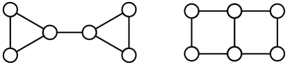
Figure 2. Two graphs that can be distinguished by SPD-SEG-WL but not WL.

Theorem 1 formally proves that SPD-SEG-WL is strictly more powerful and converges faster than WL in graph isomorphism testing. In addition to Theorem 1, we want to find out how the global structural information leveraged by shortest path encodings affects the discriminative power of SEG-WL test. We introduce the concept of receptive field of structural encodings, that when $S$ has $k$-hop receptive field, any structural information encoded by $S$ only depends on the $k$-hop neighborhood of the central node. For example, Neighbor has $1$-hop receptive field because only neighborhood connections are considered by Neighbor encoding. However, the receptive field of SPD is not restricted to $k$-hop for any $k$, since we can construct graphs with SPD between two nodes arbitrarily large. We show this global-aware receptive field brings distinctive power to SPD that differs from any encodings with local receptive field, in following Proposition 2:

Proposition 0.

For any $k$ and any structural encoding scheme $S$ with $k$-hop receptive field, there exists a pair of graphs that SPD-SEG-WL can distinguish, but $S$-SEG-WL can not.

Proof.

Let $C_{l}$ denote the cycle graph of length $l$. Then consider two graphs $G_{1}$ and $G_{2}$, where $G_{1}$ consists of $2k+4$ identical $C_{2k+3}$ graphs, and $G_{2}$ consists of $2k+3$ identical $C_{2k+4}$ graphs. $G_{1}$ and $G_{2}$ have the same number of nodes, and the induced $k$-hop neighborhood of any node in either of the two graphs is simply a path of length $2k+1$. As a result, for structural encoding scheme $S$ with $k$-hop receptive field, $S$-SEG-WL generates identical labels for every node in the two graphs, making $G_{1}$ and $G_{2}$ indistinguishable for $S$-SEG-WL. However, in $G_{2}$ there exists shortest paths of length $k+2$ while $G_{1}$ not, so SPD-SEG-WL can distinguish the two graphs. ∎

Though SPD has its unique expressive power and is more powerful than WL, many low-order non-isomorphic graphs remain to be indistinguishable by SPD-SEG-WL (see Proof for Theorem 4), which leads us to find encodings that are more powerful than SPD. Following Theorem 2, building structural encoding $S$ that satisfies $S\succeq\textit{SPD}$ can be done by adding meaningful information to SPD, which illustrates the motivation for SPIS we will next introduce.

6.2. SPIS Relative Structural Encoding

From the perspective of graph theory, for two connected nodes $v,u$ in the graph, there can be multiple shortest paths connecting $v$ and $u$, and these shortest paths may be linked or have overlapping nodes. Since SPD only encodes the length of shortest paths, one intuitive idea is to enhance it with features characterizing the rich structural interactions between different shortest paths. Inspired by concepts like betweenness centrality in network analysis (Freeman, 1977), we propose the concept of shortest path induced subgraph (SPIS) to characterize the structural relations between nodes on shortest paths:

Definition 6.0 (Shortest Path Induced Subgraph).

For $G=(V,E)$ and $v,u\in V$, $\text{SPIS}(v,u)=(V_{\text{SPIS}(v,u)},E_{\text{SPIS}(v,u)})$, the shortest path induced subgraph between $v$ and $u$ is an induced subgraph of $G$, where

(15) $$V_{\text{SPIS}(v,u)}=\{s:s\in V\text{ and }\text{SPD}_{R}(v,s)+\text{SPD}_{R}(s,u)=\text{SPD}_{R}(v,u)\}.$$

$\text{SPIS}(v,u)$ is an induced subgraph of $G$ that contains all nodes on shortest paths between $v$ and $u$. To encode knowledge in SPIS as numerical vectors, we propose the relative encoding method $\textit{SPIS}_{R}$ by enhancing $\textit{SPD}_{R}$ with the total numbers of nodes and edges of SPIS between nodes, as

(16) $$\textit{SPIS}_{R}(v,u,G)=(\textit{SPD}_{R}(v,u,G),|V_{\textit{SPIS}(v,u)}|,|E_{\textit{SPIS}(v,u)}|),$$

and we define the structural encoding scheme $\textit{SPIS}=(\textit{id}_{A},\textit{SPIS}_{R})$.

6.3. Analysis on SPIS Encoding

In the following, we will analyze the proposed SPIS encoding and characterize its mathematical properties, comparing it with SPD and WL. To start with, as SPIS is constructed by adding information to SPD, we have $\textit{SPIS}\succeq\textit{SPD}$ and it is be more powerful than SPD-SEG-WL according to Theorem 2.

Theorem 4.

(1) SPIS-SEG-WL is strictly more expressive than SPD-SEG-WL in testing non-isomorphic graphs.

(2) For $G_{1}$ and $G_{2}$ that SPD-SEG-WL distinguishes as non-isomorphic after $t$ iterations, SPIS-SEG-WL can distinguish $G_{1}$ and $G_{2}$ as non-isomorphic within $t$ iterations.

Proof.

Considering $\textit{SPD}_{R}$ is the first dimension of $\textit{SPIS}_{R}$, we have $\textit{SPIS}\succeq\textit{SPD}$ and we can prove SPIS-SEG-WL is more powerful than SPD-SEG-WL according to Theorem 2.

Figure 6 below shows a pair of graphs that can be distinguished by SPIS-SEG-WL but not SPD-SEG-WL. It is trivial to verify that SPD-SEG-WL can not distinguish them. For SPIS-SEG-WL, to understand this, Figure 6 colors examples of SPIS between non-adjacent nodes in the two graphs, where the nodes at two endpoints are colored as red. In the first graph, every SPIS between non-adjacent nodes has 3 nodes, but in the second graph there exists SPIS between non-adjacent nodes that has 4 nodes, so SPIS-SEG-WL can distinguish them. ∎

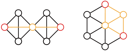
Figure 3. Two graphs that can be distinguished by SPIS-SEG-WL but not SPD-SEG-WL.

Next, we show that SPIS-SEG-WL exhibits far superior performance to WL and SPD-SEG-WL on important graph structures. The computational complexity of SPIS is discussed in Appendix B.

SPIS-SEG-WL Distinguishes All Low-order Graphs ($n\leq 8$).

On low-order graphs, our synthetic experiments in Table 1 confirm that SPIS-SEG-WL distinguishes all non-isomorphic graphs with order equal to or less than 8, which is much more powerful than WL with 332 indistinguishable pairs and SPD-SEG-WL with 200 indistinguishable pairs. This strong discriminative power on low-order graphs shows that SPIS can accurately distinguish local structures in real-world graphs.

SPIS-SEG-WL Well Distinguishes Strongly Regular Graphs.

A regular graph is a graph parameterized by two parameters $n,k$ which has $n$ nodes and each node has the $k$ neighbors, denoted as $\text{RG}(n,k)$. And a strongly regular graph parameterized by four parameters $(n,k,\lambda,\mu)$ is a regular graph $\text{RG}(n,k)$ where every adjacent pair of nodes has the same number $\lambda$ of neighbors in common, and every non-adjacent pair of nodes has the same number $\mu$ of neighbors in common, denoted as $\text{SRG}(n,k,\lambda,\mu)$.

Due to their highly symmetric structure, regular graphs are known to be failure cases for graph isomorphism test algorithms. For example, WL can not discriminate any regular graphs of the same parameters, making any pair of strongly regular graphs with the same $n$ and $k$ indistinguishable to it, even $\lambda$ and $\mu$ could be different. Yet Proposition 5 guarantees that SPIS-SEG-WL can distinguish any pair of strongly regular graphs of different parameters:

Proposition 0.

SPIS-SEG-WL can distinguish any pair of strongly regular graphs of different parameters.

Proof.

It is trivial to verify that regular graphs with different parameters can be distinguished by WL, so we focus on strongly regular graphs with the same $n$ and $k$ but different $\lambda$ and $\mu$. For $\text{SRG}(n,k,\lambda,\mu)$, since every non-adjacent pair of nodes has $\mu$ neighbors in common, the SPIS between evry non-adjacent pair of nodes will have $\mu+2$ nodes, which implies that SPIS-SEG-WL can distinguish strongly regular graphs with different $n,k,\mu$. Besides, the four parameters of strongly regular graphs are not independent, they satisfy

(17) $$\lambda=k-1-\frac{\mu}{k}(n-k-1),$$

so SPIS-SEG-WL can distinguish strongly regular graphs with different parameters. ∎

It is worth mentioning that, for strongly regular graphs with the same parameters, SPIS also exhibits outstanding discriminative power, with the number of total failures being far less than WL and SPD-SEG-WL (See Section 7.1 and Table 1).

SPIS-SEG-WL Distinguishes 3-WL Failure Cases.

When compared with $k$-order WL tests ($k\geq 3$, SEG-WL test costs only $O(n^{2})$ time complexity at each iteration, and the flexible choice of structural encoding method allows it to show a wide range of expressive capabilities. Here, we show that SPIS-SEG-WL is able to distinguish a pair of graphs that 3-WL can not distinguish:

Proposition 0.

There exists a pair of graphs that SPIS-SEG-WL can distinguish, but 3-WL can not.

Proof.

Figure 7 below shows a pair of graphs that can be distinguished by SPIS-SEG-WL but not 3-WL. The two graphs, named as the Shrikhande graph and the Rook’s $4\times 4$ graph, are both $\text{SRG}(16,6,2,2)$ and the most popular example for indistinguishability with 3-WL (Arvind et al., 2020). To show they can be distinguished by SPIS-SEG-WL, Figure 7 also colors examples of SPIS between non-adjacent nodes, where the nodes at two endpoints are colored as red. In the second graph (the Shrikhande graph), one can verify that every SPIS between non-adjacent nodes has 4 nodes and 4 edges, but in the first graph (the Rook’s $4\times 4$ graph) there exists SPIS between non-adjacent nodes that has 5 edges, making SPIS-SEG-WL capable of distinguishing them. ∎

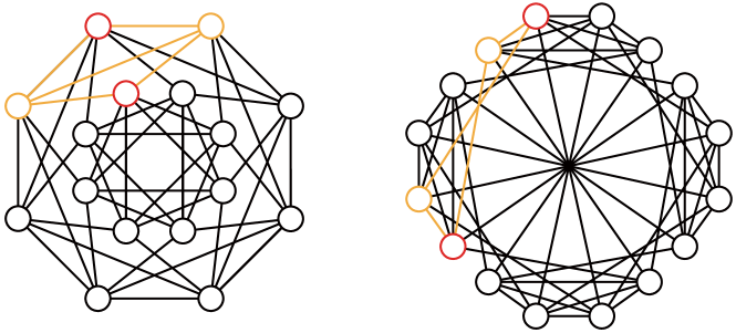
Figure 4. Two graphs (the Shrikhande graph and the Rook’s $4\times 4$ graph) that can be distinguished by SPIS-SEG-WL but not 3-WL.

Computing SPIS.

To compute SPIS encoding on a input graph $G=(V,E)$, we first use the Floyd-Warshall algorithm (Floyd, 1962) to compute the lengths of shortest paths between all pairs of vertices in $G$, which takes $O(n^{3})$ time complexity where $n=|V|$. Next for every pair of nodes $(v,u)$, for every node $s$ we test if $s$ is in $\text{SPIS}(v,u)$ by checking if $\text{SPD}_{R}(v,s)+\text{SPD}_{R}(s,u)=\text{SPD}_{R}(v,u)$ holds to construct $V_{\text{SPIS}(v,u)}$, and this step also has $O(n^{3})$ time complexity. Finally, for every pair of nodes $(v,u)$ we construct $E_{\text{SPIS}(v,u)}$ by computing the intersection between $V_{\text{SPIS}(v,u)}\times V_{\text{SPIS}(v,u)}$ and $E$. If we denote the average number of nodes of SPISs in the graph as $t$, then $V_{\text{SPIS}(v,u)}\times V_{\text{SPIS}(v,u)}$ can have $t^{2}$ edges in average and thus the final step costs $O(n^{2}t^{2})$ complexity. The overall time complexity for computing SPIS is then $O(n^{3}+n^{2}t^{2})$. As we can reasonably expect $t^{2}\sim n$ on most real-world sparse graphs because SPISs should be small with respect to the entire graph, the complexity of SPIS can be viewed as $O(n^{3})$. This is quite acceptable because the time complexity for computing SPD via Floyd-Warshall algorithm is already $O(n^{3})$, and SPIS offers a much stronger expressive power.

Low-Order Graphs (Parameter: $n$) Strongly Regular Graphs (Parameter: $(n,k,\lambda,\mu)$) Parameter $5$ $6$ $7$ $8$ $(25,12,5,6)$ $(26,10,3,4)$ $(29,14,6,7)$ $(36,14,4,6)$ $(40,12,2,4)$ $(45,12,3,3)$ # Graphs 21 112 853 11117 15 10 41 180 28 78 # Graph Pairs 210 6216 363378 61788286 105 45 820 16110 378 3003 Method # Indistinguishable Graph Pairs WL 0 3 17 312 105 45 820 16110 378 3003 SPD-SEG-WL 0 2 12 186 105 45 820 16110 378 3003 SPIS-SEG-WL 0 0 0 0 0 0 0 15 3 0

Table 1. Results of synthetic graph isomorphism tests.

Task Regression Classification Dataset ZINC QM9 QM8 ESOL PTC-MR MUTAG COX2 PROTEINS Metric MAE$\downarrow$ Multi-MAE$\downarrow$ RMSE$\downarrow$ Accuracy$\uparrow$ Method Results GCN 0.469$\pm$0.002 1.006$\pm$0.020 0.0279$\pm$0.0001 0.564$\pm$0.015 67.97$\pm$6.49 85.76$\pm$8.75 80.42$\pm$5.23 76.00$\pm$3.20 GAT 0.463$\pm$0.002 1.112$\pm$0.018 0.0317$\pm$0.0001 0.552$\pm$0.007 67.21$\pm$2.50 84.59$\pm$6.30 79.36$\pm$7.23 71.15$\pm$7.12 GIN 0.408$\pm$0.008 1.225$\pm$0.055 0.0276$\pm$0.0001 0.626$\pm$0.017 68.27$\pm$5.11 89.40$\pm$5.40 82.57$\pm$4.55 75.90$\pm$2.80 GraphSAGE 0.410$\pm$0.005 0.855$\pm$0.002 0.0275$\pm$0.0001 0.601$\pm$0.008 60.53$\pm$5.24 85.10$\pm$7.60 78.07$\pm$7.07 75.90$\pm$3.20 GSN 0.140$\pm$0.006 - - - 67.40$\pm$5.70 92.20$\pm$7.50 - 74.60$\pm$5.00 PNA 0.320$\pm$0.032 - - - - - - - 1-2-3-GNN - - - - 60.90 86.10 - 75.50 MoleculeNet - 2.350 0.0150 0.580 - - - - WL - - - - 59.90$\pm$4.30 90.40$\pm$5.70 - 75.00$\pm$3.10 RetGK - - - - 62.50$\pm$1.60 90.30$\pm$1.10 80.10$\pm$0.90 76.20$\pm$0.50 P-WL - - - - 64.02$\pm$0.82 90.51$\pm$1.34 - 75.31$\pm$0.73 FGW - - - - 65.31$\pm$7.90 88.42$\pm$5.67 77.23$\pm$4.86 74.55$\pm$2.74 GT 0.226$\pm 0.01$ - - - - - - - SAN 0.139$\pm 0.01$ - - - - - - - SAT 0.135 - - - - - - - Graphormer-id 0.668$\pm$0.003 3.176$\pm$0.005 0.0144$\pm$0.0003 0.612$\pm$0.002 66.39$\pm$5.18 85.49$\pm$8.51 77.60$\pm$7.69 77.19$\pm$4.07 Graphormer-Neighbor 0.531$\pm$0.004 1.799$\pm$0.002 0.0141$\pm$0.0002 0.639$\pm$0.034 68.13$\pm$6.82 90.35$\pm$7.01 78.06$\pm$7.43 78.12$\pm$3.62 Graphormer-SPD 0.122$\pm$0.001 0.607$\pm$0.002 0.0079$\pm$0.0001 0.492$\pm$0.004 68.43$\pm$5.82 91.39$\pm$7.35 82.12$\pm$3.40 78.59$\pm$4.35 Graphormer-SPIS 0.115$\pm$0.001 0.595$\pm$0.001 0.0073$\pm$0.0001 0.484$\pm$0.005 69.28$\pm$5.34 92.48$\pm$5.87 83.22$\pm$2.25 79.41$\pm$1.46

Table 2. Results of graph representation learning benchmarks. All results except for GCN, GAT, GIN, GraphSAGE, SAT and Graphormer variants are cited from their original papers. $\downarrow$ for lower is better, and $\uparrow$ for higher is better. Appendix D.3 reports performances on QM9 by seperate tasks.

7. Experiments

In this section, we first perform synthetic isomorphism tests on low order graphs and strongly regular graphs to evaluate the expressive power of proposed SPIS encoding against several previous benchmark methods. Then we show that by replacing SPD encoding with the provably stronger SPIS, the performance of the well-tested Graphormer model on a wide range of real-world datasets can be significantly improved.

7.1. Synthetic Isomorphism Tests

Settings.

To evaluate the structural expressive power of WL test and SEG-WL test with structural encodings described above, we first perform synthetic isomorphism tests on a collection of connected low-order graphs up to 8 nodes and strongly regular graphs up to 45 nodes. We run the algorithms above and check how they can disambiguate non-isomorphic low order graphs with the same number of nodes and strongly regular graphs with the same parameters. The results are shown in Table 1.

Results.

For low order graphs, results in Table 1 show that SPD-SEG-WL can distinguish more non-isomorphic graphs than WL, but neither can match the effectiveness of SPIS-SEG-WL which disambiguates any low-order graphs up to 8 nodes. As for the highly symmetric strongly regular graphs, both WL and SPD-SEG-WL cannot discriminate any strongly regular graphs with the same parameters, yet SPIS-SEG-WL only has few indistinguishable pairs. Compared with WL and SPD-SEG-WL, SPIS-SEG-WL has outstanding structural expressive power. Since many real-world graphs (like molecular graphs) consist of small motifs with highly symmetrical structures, it is reasonable to expect that graph Transformers with SPIS can accurately capture significant graph structures and exhibit strong discriminative power.

7.2. Graph Representation Learning

Datasets.

To test the real-world performance of graph Transformers with proposed structural encodings, we select 8 popular graph representation learning benchmarks: 5 property regression datasets (ogb-PCQM4Mv2 (Hu et al., 2021; Hu et al., 2020), ZINC(subset) (Irwin and Shoichet, 2005; Dwivedi et al., 2020), QM9, QM8, ESOL (Wu et al., 2018)) and 4 classification datasets (PTC-MR, MUTAG, COX2, PROTEINS (Morris et al., 2020a)). Statistics of the datasets are summarized the appendix. ogb-PCQM4Mv2 is a large-scale graph regression dataset with over 3 million graphs. The ZINC dataset from benchmarking-gnn (Dwivedi et al., 2020) is a subset of the ZINC chemical database (Irwin and Shoichet, 2005) with 12000 molecules, and the task is to predict the solubility of molecules. We follow the guidelines and use the predefined split for training, validation and testing. QM9 and QM8 (Ruddigkeit et al., 2012; Ramakrishnan et al., 2014, 2015) are two molecular datasets containing small organic molecules up to 9 and 8 heavy atoms, and the task is to predict molecular properties calculated with ab initio Density Functional Theory (DFT). We follow the guidelines in MoleculeNet (Wu et al., 2018) for choosing regression tasks and metrics. We perform joint training on 12 tasks for QM9 and 16 tasks for QM8. ESOL is also a molecular regression dataset in MoleculeNet containing water solubility data for compounds. PTC-MR, MUTAG, COX2 and PROTEINS are four graph classification datasets collected from TUDataset (Morris et al., 2020a). On graph regression datasets, We use random 8:1:1 split for training, validation, and testing except for ZINC, and report the performance averaged over 3 runs. On graph classification datasets, we use 10-fold cross validation with 90% training and 10% testing, and report the mean best accuracy.

Settings and Baselines.

To investigate how the expressive power of structural encodings affects the benchmark performance of real graph Transformers, we first choose the Graphormer (Ying et al., 2021) as the backbone model for testing structural encoding since Graphormer proposes SPD, which we have characterized and has expressivity stronger than WL, and the way Graphormer introduces relative structural encodings can correspond to our Theorem 3 which analyzes a simple Transformer network incorporating relative encodings via attention biases. The original Graphormer utilizes a $\textit{SPD}_{R}$ relative structural encoding (discussed in Appendix C), so we name it as Graphormer-SPD. We build a new Graphormer-SPIS model by replacing the $\textit{SPD}_{R}$ encoding with $\textit{SPIS}_{R}$ encoding as an improved version of Graphormer while keeping other network components unchanged. Similarly, we use Graphormer-id and Graphormer-Neighbor as less expressive Graphormer variants. We also include the GraphGPS (Rampášek et al., 2022) model and its variants GraphGPS-SPD and GraphGPS-SPIS into comparison on the large-scale ogbn-PCQM4Mv2 dataset with over 3 million graphs. The Transformer module in the basic GraphGPS model does not incorporate structural encoding, thus it can be considered as including id structural encoding. We construct versions of the GraphGPS model incorporating Neighbor, SPD, and SPIS structural encodings via attention biases to validate the impact of structural encoding expressivity on performance for large-scale graph tasks.

In addition, we compare the above Graphormer variants against (i) GNNs including GCN (Kipf and Welling, 2016), GIN (Xu et al., 2018), GAT (Veličković et al., 2017), GraphSAGE (Hamilton et al., 2018), GSN (Bouritsas et al., 2022), PNA (Corso et al., 2020) and 1-2-3-GNN (Morris et al., 2019); (ii) best performances collected by MoleculeNet paper (Wu et al., 2018); (iii) graph kernel based methods including WL subtree kernel (Shervashidze et al., 2011), RetGK (Zhang et al., 2018), P-WL (Rieck et al., 2019) and FGW (Titouan et al., 2019); (iv) graph Transformers including GT (Dwivedi and Bresson, 2020), SAN (Kreuzer et al., 2021), SAT (Chen et al., 2022), GRPE (Park et al., 2022) and EGT (Hussain et al., 2022). One can find the detailed descriptions of Graphormer variants, baselines, and training settings in Appendix D.2.

Model	Training MAE	Validation MAE
GCN	n/a	0.1379
GCN-virtual	n/a	0.1153
GIN	n/a	0.1195
GIN-virtual	n/a	0.1083
GRPE	n/a	0.0890
EGT	n/a	0.0869
Graphormer (-SPD)	0.0348	0.0864
Graphormer-SPIS	0.0350	0.0861
GraphGPS (medium) (-id)	0.0726	0.0858
GraphGPS-Neighbor	0.0730	0.0856
GraphGPS-SPD	0.0719	0.0853
GraphGPS-SPIS	0.0710	0.0850

Table 3. Results on ogb-PCQM4Mv2 dataset.

Results.

Table 2 and 3 presents the results of graph representation learning benchmarks. It can be observed that the performances of Graphormer variants mostly align with their relative ranking of expressive power (SPIS $\succeq$ SPD $\succeq$ Neighbor $\succeq$ id), and replacing the SPD encoding in Graphormer with the proposed stronger SPIS encoding results in a consistent performance improvement, demonstrating that real-world performance of graph Transformers can benefit from theoretically expressive structural encoding designs. Equipped with the provably powerful SPIS encoding, Graphormer-SPIS achieves state-of-the-art performance and outperforms existing graph Transformers and GNNs, which echoes our theoretical results on the strong expressive power of SPIS. Meanwhile, when employing the less expressive Neighbor and id encoding, the Transformer network loses the ability to accurately distinguish graph structures, leading to a significant performance drop. In the case of the GraphGPS model, the experimental results follow the same pattern. The original model achieved a certain level of performance improvement after incorporating the structural encoding in the Transformer layer. The stronger the expression ability of the structural encoding, the more significant the performance improvement. Overall, the experimental results demonstrate that our theoretical analysis has a practical impact on enhancing the performance of graph Transformers in various graph tasks.

8. Conclusion

In this paper, we introduce SEG-WL test as a novel unified framework for analyzing the expressive power of graph Transformers. In this framework, we theoretically characterize how to improve the expressivity of graph Transformers with respect to WL test and GNNs, and propose a provably powerful structural encoding method SPIS. Experiments have verified that the performances of benchmark graph Transformers can benefit from this theory-oriented extension. We also discuss our work’s limitations and potential social impact in Appendix E.

Appendix A Proofs

A.1. Theorem 2

We first restate Theorem 2 in a more generalized version which can be applied to both cases when the graph embedding is computed by a global readout function or virtual node trick:

Theorem 1.

For any structural encoding scheme $S=(f_{A},f_{R})$ and labeled graph $G=(V,E)$ with label map $h_{0}:V\to{\mathcal{X}}$, if a graph neural model ${\mathcal{A}}:{\mathcal{G}}\to\mathbb{R}^{d}$ satisfies the following conditions:

1. ${\mathcal{A}}$ computes the initial node embeddings with

   (18) $$l_{0}(v)=\phi(h_{0}(v),f_{A}(v,G)),$$

2. ${\mathcal{A}}$ aggregates and updates node embeddings iteratively with

   (19) $$l_{t}(v)=\sigma(\{\mskip-5.0mu\{(l_{t-1}(u),f_{R}(v,u,G)):u\in V\}\mskip-5.0mu\}),$$

   where $\phi$ and $\sigma$ above are model-specific functions,

3. The final graph embedding is computed by a global readout on the multiset of node features $\{\mskip-5.0mu\{l_{t}(v):v\in V\}\mskip-5.0mu\}$, or represented by the embedding of node $s$ such that for any $u,v\in V$, $f_{R}(s,v,G)=f_{R}(s,u,G)=f_{R}(v,s,G)=f_{R}(u,s,G)$.

then for any labeled graphs $G_{1}$ and $G_{2}$, if ${\mathcal{A}}$ maps them to different embeddings, $S$-SEG-WL also decides $G_{1}$ and $G_{2}$ are not isomorphic.

Proof.

We first show that for any node $v,u$ at iteration $t$, if $S$-SEG-WL generates $g_{t}(v)=g_{t}(u)$, then ${\mathcal{A}}$ also generates the same embeddings for $v$ and $u$ as $l_{t}(v)=l_{t}(u)$. For $t=0$ this proposition holds because if $g_{0}(v)=g_{0}(u)$ then $v$ and $u$ must have the same input label and absolute structural encoding, which leads to $l_{0}(v)=l_{0}(u)$. Suppose this proposition holds for iteration $0,1,\ldots,t$ and $g_{t+1}(v)=g_{t+1}(u)$. From the injectiveness of function $\Phi$, we have

(20) $$\{\mskip-5.0mu\{(g_{t}(r),f_{R}(v,r,G)):r\in V_{v}\}\mskip-5.0mu\}=\{\mskip-5.0mu\{(g_{t}(r),f_{R}(u,r,G)):r\in V_{u}\}\mskip-5.0mu\},$$

where $V_{v}$ is the node set of graph that $v$ belongs to, which is the same for $V_{u}$. If two finite multisets are identical, then the elements in the two multisets can be matched in pairs. Therefore, according to our assumption at iteration $t$ such that $g_{t}(v)=g_{t}(u)\implies l_{t}(v)=l_{t}(u)$, we have

(21) $$\{\mskip-5.0mu\{(l_{t}(r),f_{R}(v,r,G)):r\in V\}\mskip-5.0mu\}=\{\mskip-5.0mu\{(l_{t}(r),f_{R}(u,r,G)):r\in V\}\mskip-5.0mu\}.$$

Considering ${\mathcal{A}}$ updates node labels by $l_{t+1}(v)=\sigma(\{\mskip-5.0mu\{(l_{t}(r),f_{R}(v,r,G)):r\in V\}\mskip-5.0mu\})$, $l_{t+1}(v)=l_{t+1}(u)$ holds. This proves the proposition above by induction. Now that for any iteration $t$ we have $g_{t}(v)=g_{t}(u)\implies l_{t}(v)=l_{t}(u)$, indicating that a mapping $\psi_{t}$ exists such that for any node $v$, $l_{t}(v)=\psi_{t}(g_{t}(v))$.

Now consider two graphs $G_{1}$ and $G_{2}$ where ${\mathcal{A}}$ maps them to different embeddings after $t$ iterations. If ${\mathcal{A}}$ computes the graph embedding by a readout function on the multiset of node features, then $\{\mskip-5.0mu\{l_{t}(r):r\in V\}\mskip-5.0mu\}$ must be different for two graphs. Since $\{\mskip-5.0mu\{l_{t}(r):r\in V\}\mskip-5.0mu\}=\{\mskip-5.0mu\{\psi_{i}(g_{t}(r)):r\in V\}\mskip-5.0mu\}$, $\{\mskip-5.0mu\{g_{t}(r):r\in V\}\mskip-5.0mu\}$ must also be different for two graphs, which shows that $S$-SEG-WL decides $G_{1}$ and $G_{2}$ are not isomorphic. Meanwhile, if the graph embedding is represented by embedding of node $s$ such that for any $u,v\in V$, $f_{R}(s,v,G)=f_{R}(s,u,G)=f_{R}(v,s,G)=f_{R}(u,s,G)$, then $l_{t}(s)$ is different for two graphs. Since $l_{t}(s)$ is generated by $l_{t}(s)=\sigma(\{\mskip-5.0mu\{(l_{t-1}(r),f_{R}(s,r,G)):r\in V\}\mskip-5.0mu\})$ and $f_{R}(s,r,G)$ is the same for every $r\in V$, $\{\mskip-5.0mu\{l_{t-1}(r):r\in V\}\mskip-5.0mu\}$ must be different for two graphs, which goes back to the situation we have discussed above. Therefore, the proof is completed. ∎

A.2. Theorem 3

Our proof for Theorem 3 is largely based on the proof for the universal approximation theorem of the Transformer architecture, so it is strongly recommended to go through the proof in (Yun et al., 2019) before reading our proof in the next section.

A.2.1. bias-GT Model

To present a simple and flexible example on building theoretically powerful graph Transformers, we propose bias-GT, a graph Transformer model that works under any structural encoding schemes with minimal modifications to the original Transformer architecture. More concretely, for $S=(f_{A},f_{R})$ and input graph $G$, the input embedding of node $v$ is computed by

(22) $$l_{0}(v)=\text{Linear}(\text{Concat}(h_{0}(v),f_{A}(v,G)),$$

where Linear$(\cdot)$ is a linear layer, Concat$(\cdot)$ refers to the concatenation operation. At every Transformer layer, the relative structural encodings are introduced as transformed attention biases. For every node pair $(u,v)$, the final attention weight $a_{uv}$ from node $u$ to $v$ is computed by

(23) $$a_{uv}=\bar{a}_{uv}+\text{Embedding}(f_{R}(u,v,G)),$$

where $\bar{a}_{uv}$ is the original attention weight computed by scaled-dot self-attention, and $\text{Embedding}(\cdot)$ transforms relative embeddings in ${\mathcal{C}}$ to $\mathbb{R}$ using via embedding lookup or linear layers. All remaining network components stay the same with the original Transformer architecture. This bias-GT model offers a straightforward strategy for injecting strutural information to the Transformer and can be viewed as a simplified version of some exisiting models (Ying et al., 2021; Zhao et al., 2021). We will use $S$-bias-GT to denote bias-GT network with structural encoding scheme $S$. The proposition below shows that $S$-SEG-WL test limits the expressive power of $S$-bias-GT:

Proposition 0.

For any regular structural encoding scheme $S=(f_{A},f_{R})$ and two graphs $G_{1},G_{2}$, if $S$-bias-GT maps them to different embeddings, $S$-SEG-WL also decides $G_{1}$ and $G_{2}$ are not isomorphic.

Proof.

We only need to check the conditions in Theorem 2. For the first condition, $S$-bias-GT computes the initial node embeddings with

(24) $$l_{0}(v)=\phi(h_{0}(v),f_{A}(v,G))=\text{Linear}(\text{Concat}(\bar{h}_{0}(v),f_{A}(v,G)),$$

and for the second condition, since $S$ is regular, the relative structural encoding functions satisfy $f_{R}(v,v,G)\neq f_{R}(v,u,G)$ for $v,u\in V$, then a function operated on $\{\mskip-5.0mu\{(l_{t-1}(u),f_{R}(v,u,G)):u\in V\}\mskip-5.0mu\}$ can be viewed as a function operated on $(h_{v},\{\mskip-5.0mu\{(l_{t-1}(u),f_{R}(v,u,G)):u\in V\}\mskip-5.0mu\})$ because $f_{R}(v,v,G)$ is different from all other relative encodings. $S$-bias-GT updatesthe node embeddings with

(25) $$l_{t}(v)= \sigma(h_{v},\{\mskip-5.0mu\{(l_{t-1}(u),f_{R}(v,u,G)):u\in V\}\mskip-5.0mu\})$$

(26) $$= \text{FFN}({\text{Concat}}_{i=1,\ldots,h}({\sum_{u\in V}}w_{vu}^{i}l_{t-1}(v)W^{i}_{Q})W_{O}),$$

(27) $$\text{where }w_{vu}^{i}=\frac{\text{exp}(\bar{\alpha}_{vu}^{i})}{\sum_{r\in V}\text{exp}(\bar{\alpha}_{vr}^{i})}$$

(28) $$\text{and }\bar{\alpha}_{vu}^{i}=\frac{(l_{t-1}(v)W_{Q}^{i})(l_{t-1}(u)W_{K}^{i})^{\top}}{\sqrt{d}}$$

(29) $$\quad+\text{Embedding}_{i}(f_{R}(v,u,G)).$$

$W_{Q}^{i},W_{K}^{i},W_{V}^{i},W_{O}$ above are projection matrices, FFN is the feed-forward layer, and layer normalization and residual connections are omitted for clarity. The function $\sigma$ is basically the computation steps of the Transformer with $f_{R}(v,u,G)$ injected as attention bias. Since the graph embedding can be computed by a global readout function, according to Theorem 2, the proof is completed. ∎

A.2.2. Explainations on Theorem 3

When the input graph order $n$ is fixed, let the input be $G=(V,E)$ with label map $h_{0}$ and $V=\{v_{1},\ldots,v_{n}\}$. To properly define this approximation process, for some structural encoding scheme $S$, the input for both SEG-WL test and bias-GT network $g$ is viewed as the feature matrix ${\bm{X}}_{0}=[h_{0}(v_{1}),\ldots,h_{0}(v_{n})]\in\mathbb{R}^{d\times n}$ and the adjacency matrix ${\bm{A}}$ with permutation invariance. We define the SEG-WL test function $f_{t}$ by stacking all labels generated by $t$-iteration SEG-WL test in $f_{t}({\bm{X}}_{0},{\bm{A}})=[g_{t}(v_{1}),\ldots,g_{t}(v_{n})]$, and the output of $g$ is similarly defined by stacking all feature vectors generated by the network. We define the $\mathsf{d}_{p}$ distance between $f_{t}$ and $g$ as $\mathsf{d}_{p}(f_{t},g)=\max_{{\bm{A}}}\mathsf{d}_{p}(f_{t}(\cdot,{\bm{A}}),g(\cdot,{\bm{A}}))$, where $\mathsf{d}_{p}(f_{t}(\cdot,{\bm{A}}),g(\cdot,{\bm{A}}))$ is the $\ell^{p}$ distance on $\mathbb{R}^{d\times n}$ between $f_{t}$ and $g$ when ${\bm{A}}$ is fixed. Following (Yun et al., 2019), $\mathsf{d}_{p}$ also stands for $\ell^{p}$ distance between functions in the remaining context.

$\Phi(\{\mskip-5.0mu\{(g_{t-1}(v_{i}),f_{R}(v_{j},v_{i},G)):v_{i}\in V)\}\mskip-5.0mu\})$ can be viewed as a permutation (of node order) invariant function $\Phi({\bm{X}}_{t-1},{\bm{W}}_{j})$, where ${\bm{X}}_{t-1}=[g_{t-1}(v_{1}),\ldots,g_{t-1}(v_{n})]\in\mathbb{R}^{d\times n}$ is the matrix of node labels and ${\bm{W}}_{j}=[f_{R}(v_{j},v_{1},G)),\ldots,f_{R}(v_{j},v_{n},G))]\in{\mathcal{C}}^{n}$. The assumption that $\Phi$ can be extended to a continuous function with respect to node labels means that, for any fixed ${\bm{W}}_{j}$, $\Phi({\bm{X}}_{t-1},{\bm{W}}_{j})$ is a continuous function with respect to any entry-wise $\ell^{p}$ norm of ${\bm{X}}_{t-1}$ with compact support in $\mathbb{R}^{d\times n}$ (since ${\mathcal{X}}$ is compact).

A.2.3. Proof for Theorem 3

Proof.

Since the first iteration of SEG-WL test can be arbitrarily approximated by performing a linear layer on embeddings generated by concatnating the initial embeddings and absolute positional encodings, according to the universal approximation theorem (Hornik et al., 1989) and Lipschitz continuity of feed-forward layers, the key technical challenge in proving Theorem 3 is showing that each iteration $i$ in $1,\ldots,t$ of SEG-WL test can be approximated arbitrarily well using the bias-GT network. Let $f$ stands for one iteration of $S$-SEG-WL test, with input and output defined according to $f_{t}$. We denote $\bm{\alpha}_{i,j}=f_{R}(v_{i},v_{j},G)$ for simplicity, and let ${\bm{x}}_{i}$ be the input labels of $v_{i}$ for $f$. Then $f$ can be viewed as:

(30) $$f({\bm{X}},{\bm{A}})=[\Phi(\{\mskip-5.0mu\{({\bm{x}}_{i},\bm{\alpha}_{1,i})\}\mskip-5.0mu\}_{i=1,\ldots,n}),\ldots,\Phi(\{\mskip-5.0mu\{({\bm{x}}_{i},\bm{\alpha}_{n,i})\}\mskip-5.0mu\}_{i=1,\ldots,n})].$$

That is, if our Transformer network is capable of approximating the multiset function $\Phi$ that takes the feature matrix and structural encodings as input, then it can approximate $f$ at any precision because the output of $f$ contains $n$ entries computed individually by $\Phi$. As we have mentioned, $\Phi$ can be rewritten to the following equivalent form:

(31) $$\Phi(\{\mskip-5.0mu\{({\bm{x}}_{i},\bm{\alpha}_{j,i})\}\mskip-5.0mu\}_{i=1,\ldots,n})=\Phi({\bm{X}},{\bm{W}}_{j}),\text{ where }{\bm{X}}=[{\bm{x}}_{1},\ldots,{\bm{x}}_{n}]$$

(32) $$\text{ and }{\bm{W}}_{j}=[\bm{\alpha}_{j,1},\ldots,\bm{\alpha}_{j,n}].$$

In this form, $\Phi$ is permutation equivariant such that for any permutation matrix ${\bm{P}}$, $\Phi({\bm{X}}{\bm{P}},{\bm{W}}_{j}{\bm{P}})=\Phi({\bm{X}},{\bm{W}}_{j})$.

The major problem is that the bias-GT network $g$ only take ${\bm{X}}$ as feature input while incorporating structural encodings ${\bm{W}}_{j}$ in attention layers as biases. According to our assumptions, we can assume without generality that ${\mathcal{X}}\subset(0,1)^{d}$ and the compact support of extented function $\Phi$ with respect to ${\bm{X}}$ is contained within $[0,1]^{d\times n}$. We follow the proof structure outlined in (Yun et al., 2019).

Step 1: Approximate $f$ by $\bar{f}$, a piece-wise constant function with respect to ${\bm{X}}$.

According to previous assumptions and statements in (Yun et al., 2019), for any fixed ${\bm{W}}_{j}$, $\Phi$ is a uniform continuous function (because $\Phi$ has compact support) with respect to the argument ${\bm{X}}$. Suppose for ${\bm{W}}_{j}$, there exists $\delta_{{\bm{W}}_{j}}$ such that for any ${\bm{X}},{\bm{Y}}$,$\|{\bm{X}}-{\bm{Y}}\|_{\infty}<\delta_{{\bm{W}}_{j}}$ we have $\|\Phi({\bm{X}},{\bm{W}}_{j})-\Phi({\bm{Y}},{\bm{W}}_{j})\|_{p}<\frac{\epsilon}{3}$. Since the possible graph structures of order $n$ is finite, ${\mathcal{C}}$ is a finite set and the possible choices of ${\bm{W}}_{j}$ is also finite. Therefore, we can pick $\delta=\min_{{\bm{W}}_{j}}\{\delta_{{\bm{W}}_{j}}\}$, then for any ${\bm{X}},{\bm{Y}},{\bm{W}}_{j}$, if $\|{\bm{X}}-{\bm{Y}}\|_{\infty}<\delta$ we have $\|\Phi({\bm{X}},{\bm{W}}_{j})-\Phi({\bm{Y}},{\bm{W}}_{j})\|_{p}<\frac{\epsilon}{3}$. Accordingly, we can define a piece-wise constant function $\bar{\Phi}$ to approximate $\Phi$ as

(33) $$\bar{\Phi}({\bm{X}},{\bm{W}}_{j})=\sum_{{\bm{L}}\in{\mathbb{G}}_{\delta}}\Phi({\bm{C}}_{{\bm{L}}},{\bm{W}}_{j})\mathbbm{1}\{{\bm{X}}\in{\mathbb{S}}_{{\bm{L}}}\},$$

where ${\mathbb{S}}_{{\bm{L}}}$ is a cube of width $\delta$ with ${\bm{L}}$ being one of its vertices, ${\bm{C}}_{{\bm{L}}}\in{\mathbb{S}}_{{\bm{L}}}$ is the center point of ${\mathbb{S}}_{{\bm{L}}}$ (Please refer to Appendix B.1 of (Yun et al., 2019) for a detailed explanation). By the uniform continuity of $\Phi$, we can prove $\|\Phi({\bm{X}},{\bm{W}}_{j})-\bar{\Phi}({\bm{X}},{\bm{W}}_{j})\|_{p}<\frac{\epsilon}{3}$ for any ${\bm{X}},{\bm{W}}_{j}$. Also, it is trivial to verify that $\bar{\Phi}$ is permutation equivariant. By defining $\bar{f}$ by replacing function $\Phi$ with $\bar{\Phi}$ in Equation 30, we have $\mathsf{d}_{p}(f,\bar{f})\leq\frac{\epsilon}{3}.$

Step 2: Approximate $\bar{f}$ with modified bias-GT network.

In this step we aim to approximate $\bar{f}$ using a modified bias-GT network, where the softmax operator $\sigma[\cdot]$ and $\text{ReLU}(\cdot)$ are replaced by the $\gamma$-hardmax operator $\sigma_{\text{H},\gamma}[\cdot]$ and an activation finction $\phi$ that is a piece-wise linear function with at most three pieces in which at least one piece is constant. Note that the $\gamma$-hardmax operator is defined by adding $\gamma>0$ to non-zero elements of $\sigma_{\text{H}}$.

Proposition 0.

$\bar{\Phi}$ can be approximated by a modified bias-GT network $\bar{g}$ such that $\mathsf{d}_{p}(\bar{f},\bar{g})\leq\frac{\epsilon}{3}.$

Step 3: Approximate modified bias-GT network with (original) bias-GT network.

Finally, we will show that the modified bias-GT $\bar{g}$ can be approximated by the original bias-GT architecture.

Proposition 0.

$\bar{g}$ can be approximated by a bias-GT network $g$ such that $\mathsf{d}_{p}(g,\bar{g})\leq\frac{\epsilon}{3}.$

Following (Yun et al., 2019), along with three steps above, we prove that a single $S$-SEG-WL iteration $f$ can be arbitrarily approximated with a bias-GT network $g$. By stacking such bias-GT networks, we show that $S$-SEG-WL with any number of iterations can be approximated by $S$-bias-GT at any precision. We next provide proofs for the two propositions. ∎

A.2.4. Proof for Proposition 3

Proof.

We only need to notice that for any ${\bm{A}}$, $\sigma_{\text{H},\gamma}({\bm{A}})\to\sigma_{\text{H}}({\bm{A}})$ as $\gamma\to 0$. Then together with Appendix B.2 of (Yun et al., 2019), we can finish the proof. ∎

A.2.5. Proof for Proposition 4

Proof.

We will prove this statement in five major steps:

1. Given input ${\bm{X}}$, a group of feed-forward layers in the modified Transformer network can quantize ${\bm{X}}$ to an element ${\bm{L}}$ on the grid ${\mathbb{G}}_{\delta}:=\{0,\delta,\ldots,1-\delta\}^{d\times n}.$

2. A group of additional feed-forward layers then scales ${\bm{L}}$ to a different level, where for every $l_{j}:={\bm{u}}^{\top}{\bm{L}}_{:,j},$ $l_{j}\in\{1,\delta^{-1},\delta^{-2},\ldots,\delta^{-\delta^{-d}+1}\}$ holds. (${\bm{u}}=(1,\delta^{-1},\delta^{-2},\ldots,\delta^{-d+1})$.)

3. A group of biased self-attention layers perform global shift on ${\bm{L}}$, such that for any $i$ and $j$, the shifted $l_{i}$ and $l_{j}$ are different if and only if their corresponding multisets of label-RSE tuples ($\{\mskip-5.0mu\{({\bm{x}}_{k},\bm{\alpha}_{i,k}):k=1,\ldots,n\}\mskip-5.0mu\}$ for $l_{i}$) are different.

4. Next, a group of self-attention layers map the shifted ${\bm{L}}$ to the desirable contextual mappings $q({\bm{L}})$. (defined in (Yun et al., 2019))

5. Finally, a group of feed-forward layers can map elements of the contextual embeddings $q({\bm{L}})$ to the desirable values in the piece-wise constant function.

Smiliar to Section 4 of (Yun et al., 2019), Proposition 4 can be proved with five steps above, where the major difference here is in Step 1-3 we create contextual mappings for both node features and relative structural encodings. Next we explain the five steps in detail.

Step 1.

Since ${\mathcal{X}}$ is bounded, we can assume without generality that ${\mathcal{X}}\subset(0,1)^{d}$. Thus, according to Lemma 5 in (Yun et al., 2019), the input ${\bm{X}}$ can be quantized to grid ${\mathbb{G}}_{\delta}:=\{0,\delta,\ldots,1-\delta\}^{d\times n}.$ We still use ${\bm{x}}_{i}$ to denote the quantized feature vector.

Step 2.

Before this step, we have $l_{j}\in[0:\delta:\delta^{-d+1}-\delta]$. Our goal in this step is to scale each $l_{j}$ to $\delta^{-\delta^{-1}l_{j}}$. For every entry ${\bm{L}}_{:,j}$ in ${\bm{L}}$, the scaling function is defined as

(34) $${\bm{L}}_{:,j}\mapsto{\bm{L}}_{:,j}+(\delta^{-\delta^{-1}{\bm{u}}^{\top}{\bm{L}}_{:,j}}-{\bm{u}}^{\top}{\bm{L}}_{:,j}){\bm{e}}^{(1)},$$

We use a group of feed-forward layers to approximate this function, which is possible because Transformer has residual connections. Note that after this process, $\{1,\delta^{-1},\delta^{-2},\ldots,\delta^{-\delta^{-d}+1}\}$ contains all possible values for $l_{j}$. As our proof can have $\delta$ arbitrarily small, we assume $\delta^{-1}>n$.

Step 3.

Since ${\mathcal{C}}$ is finite we may assume ${\mathcal{C}}=\{1,2,\ldots,c\}$, and let ${\bm{W}}=\{\bm{\alpha}_{r,s}\}_{r,s=1,\ldots,n}$. We use one self-attention layer consists of $c$ attention heads to perform the desired global shift. We first define

(35) $$\phi_{i}({\bm{W}})=\{\phi_{i}(\bm{\alpha}_{r,s})\}_{r,s=1,\ldots,n},$$

(36) $$\text{where }\phi_{i}(x)=\begin{cases}1,\text{ if }x=i,\\ 0,\text{ else.}\end{cases}$$

Then, for $i=1,2,\ldots,c$, the $i$-th attention head is defined as

(37) $$\psi_{i}({\bm{Z}})={\bm{e}}^{(1)}{\bm{u}}^{\top}{\bm{Z}}\sigma_{\text{H},\delta^{-p+1}/n!}(\phi_{i}({\bm{W}}))$$

where $p=-\delta^{-d}$. Noticing $\lim_{\delta\to 0}\delta^{-p+1}/n!=0$ and the fact in A.2.4, the selected $\sigma_{\text{H},\delta^{-p+1}/n!}$ is acceptable. This $\phi_{i}(x)$ function can be learned by embedding layers operated on the relative structural encodings. And the final attention layer is computed as

(38) $$\Psi({\bm{Z}})={\bm{Z}}+\sum_{i=1}^{c}n!\delta^{(3p+q)i}\psi_{i}({\bm{Z}}),$$

where $q$ satisfies $\delta^{q+1}\leq n!\leq\delta^{q}$. Note that $p$ and $q$ are both negative. For the convenience of further description, we define ${\bm{u}}^{\top}\Psi({\bm{L}})=[\bar{l}_{1},\ldots,\bar{l}_{n}].$

Explanation on Step 2 and 3.

We aim to generate the bijective column id mapping for each $\{\mskip-5.0mu\{({\bm{x}}_{j},\bm{\alpha}_{i,j}):j=1,\ldots,n\}\mskip-5.0mu\}$, while using only ${\bm{X}}$ as feature input and the structural encodings are leveraged by shift operations in Step 2 and 3. We further prove this in Proposition 4 below:

Proposition 0.

For any $u,v\in\{1,\ldots,n\}$, $\bar{l}_{u}=\bar{l}_{v}$ if and only if $\{\mskip-5.0mu\{({\bm{x}}_{j},\bm{\alpha}_{u,j}):j=1,\ldots,n\}\mskip-5.0mu\}=\{\mskip-5.0mu\{({\bm{x}}_{j},\bm{\alpha}_{v,j}):j=1,\ldots,n\}\mskip-5.0mu\}$, and every $\bar{l}_{u}$ is bounded.

Proof.

For each node $u$, we define $Y(u,i)=\{\mskip-5.0mu\{{\bm{x}}_{v}:\bm{\alpha}_{u,v}=i\}\mskip-5.0mu\}$ and $S(u,i)=\sum_{\bm{\alpha}_{u,v}=i}l_{v}$, where $l_{v}$ is the scaled ${\bm{u}}^{\top}{\bm{L}}_{:,v}$ after Step 2.

Let the first row of $\psi_{i}({\bm{Z}})$ be $[r_{i}(1),r_{i}(2),\ldots,r_{i}(n)].$ We first show that $r_{i}(u)=r_{i}(v)$ if and only if $Y(u,i)=Y(v,i)$. Due to the ingenious construction of ${\bm{u}}$ in (Yun et al., 2019), $l_{j}$ has been an injective descriptor of ${\bm{x}}_{j}$ before the scaling in Step 2. Since the scaling in Step 2 is injective, the scaled $l_{j}$ also becomes an injective descriptor of ${\bm{x}}_{j}$. According to our scaling strategy, the scaled $l_{j}$ can be viewed as a $p$-digit one-hot representation of ${\bm{x}}_{j}$. Noticing $\delta^{-1}>n$, $S(u,j)$, as the summation of these scaled $l_{j}$, also becomes a unique descriptor of $Y(u,i)$ and $1\leq S(u,j)\leq\delta^{p}$.

Definition A.0.

Suppose the set of possible values of $a$ is $P$. Then for any $u,v\in P$, if $|u-v|$ is always an integer multiple of $s$, then we call $s$ the minimal distance between any unique choices of $a$.

Accordingly, the minimal distance between any unique choices of $S(u,j)$ is $1$ because the the minimal distance between any scaled $l_{j}$ is $1$.

Next, before discussing $\psi_{i}$ in Equation (37), (38) and $r_{i}$, we first present a lamma:

Lemma 0.

For real numbers $a,b$, the minimal distance between any unique choices of $b$ is $s$, and $a\leq m$ holds. $a+b$ becomes a unique descriptor of $a$ if $2m<s$.

Proof.

Suppose we have $a_{1}+b_{1}=a_{2}+b_{2}$ and $a_{1}\neq a_{2}$. Then we have

(39) $$|a_{1}-a_{2}|=|b_{1}-b_{2}|,$$

and $|b_{1}-b_{2}|\geq s$, $|a_{1}-a_{2}|\leq 2m$. Then the proof is completed by contradiction. ∎

Given the definition of $\psi_{i}$ (please refer to Appendix B.5 in (Yun et al., 2019) for more details on the selective shift operation, which is the basis for the construction of $\psi_{i}$), we have

(40) $$r_{i}(u)=(\frac{1}{k}+\frac{\delta^{-p+1}}{n!})S(u,i),$$

where $k=|Y(u,i)|$. According to the range of scaled $l_{j}$, we have

(41) $$1\leq\frac{1}{k}S(u,i)\leq\delta^{p+1},$$

(42) $$\frac{\delta^{-p+1}}{n!}\leq\frac{\delta^{-p+1}}{n!}S(u,i)\leq\frac{\delta}{n!}.$$

It is easy to infer that the minimal distance between any unique choices of $\frac{1}{k}S(u,i)$ is an integer multiple of $\frac{1}{n!}$, and we have

(43) $$2\cdot\frac{\delta}{n!}<2\cdot\frac{1}{2n!}=\frac{1}{n!}.$$

According to Lemma 6, $r_{i}(u)$ is a unique descriptor of $\frac{\delta^{-p+1}}{n!}S(u,i)$, then it is also a unique descriptor of $Y(u,j)$. Now we have $1\leq r_{i}(u)\leq\delta^{p}$ and the minimal distance between any unique choices of $r_{i}(u)$ is $\frac{\delta^{-p+1}}{n!}$. The following Lemma is applied to the construction of $\Psi$:

Lemma 0.

For $k$ positive real numbers $a_{1},a_{2},...,a_{k}$, $\sum_{i=1}^{k}a_{i}$ is a unique descriptor of $(a_{1},a_{2},\ldots,a_{k})$ if:

1. For any $a_{i}$, there exists $r_{i}$ such that $a_{i}\leq r_{i}$,

2. Let $s(i)$ be the minimal distance between any unique choices of $a_{i}$, then $s(i)>\sum_{j=1}^{i-1}r_{j}$ holds for any $i$.

Proof.

Assuming that there exists two groups of positive real numbers $\{a_{i}^{(1)}\}_{i=1}^{k}$ and $\{a_{i}^{(2)}\}_{i=1}^{k}$ which both satisfy conditions above and $\sum_{i=1}^{k}a_{i}^{(1)}=\sum_{i=1}^{k}a_{i}^{(2)}$. Besides, the two group of numbers are not totally equal correspondingly, which means there must exist one $l\in\{1,2,...,c\}$ such that $a_{l}^{(1)}\neq a_{l}^{(2)}$ and for any $j>l$, $a_{j}^{(1)}=a_{j}^{(2)}$ holds.

According to the second condition, $|a_{l}^{(1)}-a_{l}^{(2)}|>\sum_{j=1}^{l-1}r_{j}$ holds. Since $\sum_{i=1}^{k}a_{i}^{(1)}=\sum_{i=1}^{k}a_{i}^{(2)}$, then

(44) $$|a_{l}^{(1)}-a_{l}^{(2)}| =|\sum_{j=1}^{l-1}a_{j}^{(1)}-\sum_{j=1}^{l-1}a_{j}^{(2)}|$$

(45) $$=|\sum_{j=1}^{l-1}(a_{j}^{(1)}-a_{j}^{(2)})|$$

(46) $$\leq\sum_{j=1}^{l-1}|a_{j}^{(1)}-a_{j}^{(2)}|$$

(47) $$\leq\sum_{j=1}^{l-1}r_{j},$$

where the proof is completed by contradiction. ∎

Finally we consider the definition of $\Psi$. We have

(48) $$\bar{l}_{u}=l_{u}+\sum_{i=1}^{c}n!\delta^{(3p+q)i}r_{i}(u),$$

and it can be concluded that

(49) $$1\leq l_{u}\leq\delta^{p+1},$$

(50) $$\delta^{3ip+(i+1)q+1}\leq n!\delta^{(3p+q)i}r_{i}(u)\leq\delta^{(3i+1)p+(i+1)q},\text{ for }i=1,\ldots,c.$$

And the minimal distance between any unique choices of $n!\delta^{(3p+q)i}r_{i}(u)$ is

(51) $$s(i)=\delta^{(3i-1)p+iq+1}.$$

If $i=1$, then $s(1)=\delta^{2p+q+1}>\delta^{p+1}$; if $i=j+1$, then trivially we have

(52) $$s(j+1)=\delta^{(3j+2)p+(j+1)q+1}>\sum_{s=1}^{j}\delta^{(3s+1)p+(s+1)q}.$$

Thus, according to the lemma above, $\bar{l}_{u}$ also becomes a unique descriptor of $\{\mskip-5.0mu\{Y(u,i):i=1,\ldots,n\}\mskip-5.0mu\}$, then it must be a unique descriptor of $\{\mskip-5.0mu\{({\bm{x}}_{u},\bm{\alpha}_{u,j}):j=1,\ldots,n\}\mskip-5.0mu\}$. We also have $\bar{l}_{u}$ bounded as $\bar{l}_{u}<\delta^{(3c+1)p+(c+1)q-1}$, which completes the proof. ∎

Step 4.

After the previous steps, $\bar{l}_{u}$ is the unique id for $\{\mskip-5.0mu\{({\bm{x}}_{j},\bm{\alpha}_{u,j}):j=1,\ldots,n\}\mskip-5.0mu\}$, and we have $\bar{l}_{u}\in[0:\delta:\delta^{(3c+1)p+(c+1)q-1}-\delta].$ It can be observed that if we define $d^{\prime}=(3c+1)p+(c+1)q-1$ and treat $d^{\prime}$ as the "new" $d$, we can apply exactly the same methods in Appendix B.5 of (Yun et al., 2019) to employ multiple selective shift operations and generate contextual embeddings for ${\mathcal{H}}=[\{\mskip-5.0mu\{({\bm{x}}_{j},\bm{\alpha}_{i,j}):j=1,\ldots,n\}\mskip-5.0mu\}]_{i=1,\ldots,n}$. Note that since we assume ${\mathcal{X}}\subset(0,1)^{d\times n}$, only Category 1 and 2 (Appendix B.5 of (Yun et al., 2019)) need to be considered.

Step 5.

Now with contextual embeddings $q({\mathcal{H}})$, we can use methods in Appendix B.6 of (Yun et al., 2019) to map every mapping values to the desired output computed by $\bar{f}$, which completes the proof. ∎

A.3. Proof for Theorem 2

Proof.

Let the label mappings generated by $S^{\prime}$-SEG-WL and $S$-SEG-WL at iteration $t$ be $g^{\prime}_{t}$ and $g_{t}$ respectively. We denote the conditions in Equation 13 and 14 as $f_{A}=p_{A}(f_{A}^{\prime})$ and $f_{R}=p_{R}(f_{R}^{\prime})$. For graphs $G_{v}=(V_{v},E_{v})$ and $G_{u}=(V_{u},E_{u})$ ($G_{v}$ and $G_{u}$ may be the same graph), we first show that for any node $v\in V_{v}$ and $u\in V_{u}$ at iteration $t$, if $S^{\prime}$-SEG-WL generates $g_{t}^{\prime}(v)=g_{t}^{\prime}(u)$, then $S$-SEG-WL also gets $g_{t}(v)=g_{t}(u)$. For $t=0$ this holds because if $g_{0}^{\prime}(v)=g_{0}^{\prime}(u)$ then $v$ and $u$ must have $h_{0}(v)=h_{0}(u)$ and $f_{A}^{\prime}(v,G_{v})=f_{A}^{\prime}(u,G_{u})$. Since $f_{A}=p_{A}(f_{A}^{\prime})$, it means that $f_{A}(v,G_{v})=f_{A}(u,G_{u})$, which leads to $g_{0}(v)=g_{0}(u)$. Suppose this condition holds for iteration $0,1,\ldots,t$ and $g_{t+1}^{\prime}(v)=g_{t+1}^{\prime}(u)$. From the injectiveness of function $\Phi$, we have

(53) $$\{\mskip-5.0mu\{(g_{t}^{\prime}(r),f_{R}^{\prime}(v,r,G_{v})):r\in V_{v}\}\mskip-5.0mu\}=\{\mskip-5.0mu\{(g_{t}^{\prime}(r),f_{R}^{\prime}(u,r,G_{u})):r\in V_{u}\}\mskip-5.0mu\}.$$

If two finite multisets are identical, then the elements in the two multisets can be matched in pairs. The condition $f_{R}=p_{R}(f_{R}^{\prime})$ implies that for any $r,s$, $f_{R}^{\prime}(v,r,G_{v})=f_{R}^{\prime}(u,s,G_{u})\implies f_{R}(v,r,G_{v})=f_{R}(u,s,G_{u})$. Together with the assumption that $g_{t}^{\prime}(v)=g_{t}^{\prime}(u)$ implies $g_{t}(v)=g_{t}(u)$, we can conclude that

(54) $$(g_{t}^{\prime}(r),f_{R}^{\prime}(v,r,G_{v}))=(g_{t}^{\prime}(s),f_{R}^{\prime}(u,s,G_{u}))\implies$$

(55) $$(g_{t}(r),f_{R}(v,r,G_{v}))=(g_{t}(s),f_{R}(u,s,G_{u})).$$

Therefore, we have

(56) $$\{\mskip-5.0mu\{(g_{t}(r),f_{R}(v,r,G_{v})):r\in V_{v}\}\mskip-5.0mu\}=\{\mskip-5.0mu\{(g_{t}(r),f_{R}(u,r,G_{u})):r\in V_{u}\}\mskip-5.0mu\},$$

which directly leads to $g_{t+1}(v)=g_{t+1}(u)$. Then the proposition above is proved by induction. Now that for any iteration $t$ we have $g_{t}^{\prime}(v)=g_{t}^{\prime}(u)\implies g_{t}(v)=g_{t}(u)$, indicating that a mapping $\psi_{t}$ exists such that for any node $v$, $g_{t}(v)=\psi_{t}(g_{t}^{\prime}(v))$.

Now consider two graphs $G_{1}$ and $G_{2}$ where $S$-SEG-WL decides them as non-isomorphic after $t$ iterations, then the multiset of all updated node labels $\{\mskip-5.0mu\{g_{t}(v):v\in V\}\mskip-5.0mu\}$ must be different for two graphs. Since $\{\mskip-5.0mu\{g_{t}(v):v\in V\}\mskip-5.0mu\}=\{\mskip-5.0mu\{\psi_{t}(g_{t}^{\prime}(v)):v\in V\}\mskip-5.0mu\}$, $\{\mskip-5.0mu\{g_{t}^{\prime}(v):v\in V\}\mskip-5.0mu\}$ must also be different for two graphs or we will reach a contradiction, which suggests that $S^{\prime}$-SEG-WL distinguishes $G_{1}$ and $G_{2}$ after $t$ iterations. ∎

A.4. Proof for Theorem 3

Proof.

The formal definition for WL test is presented in Appendix 2. Here we denote $N^{+}(v)=N(v)\cup\{v\}$ as the ego subgraph of node $v$. For label update of node $v$, the values of $\textit{Neighbor}_{R}$ divides the node set $V$ into three parts: the central node $v$, the neighborhood nodes $N(v)$ and nodes out of $v$’s ego subgraph $V\setminus N^{+}(v)$. Thus, the node label update function controlled by $\textit{Neighbor}_{R}$ can be viewed as

(57) $$g_{t}(v)=\Phi(g_{t}(v),\{\mskip-5.0mu\{g_{t}(r):r\in N(v)\}\mskip-5.0mu\},\{\mskip-5.0mu\{g_{t}(s):s\in V\setminus N^{+}(v)\}\mskip-5.0mu\}).$$

For the first part of the proof, we prove that Neighbor-SEG-WL can distinguish any non-isomorphic graphs distinguishable by WL test. We first show that for any node $v,u$ at iteration $t$, if Neighbor-SEG-WL generates $g_{t}(v)=g_{t}(u)$, then WL will obtain $w_{t}(v)=w_{t}(u)$. For $t=0$ this obviously holds. Suppose this condition holds for iteration $0,1,\ldots,t$ and $g_{t+1}(v)=g_{t+1}(u)$. From the injectiveness of function $\Phi$, we have

(58) $$(g_{t}(v),\{\mskip-5.0mu\{g_{t}(r):r\in N(v)\}\mskip-5.0mu\},\{\mskip-5.0mu\{g_{t}(s):s\in V_{v}\setminus N^{+}(v)\}\mskip-5.0mu\})$$

(59) $$= (g_{t}(u),\{\mskip-5.0mu\{g_{t}(r):r\in N(u)\}\mskip-5.0mu\},\{\mskip-5.0mu\{g_{t}(s):s\in V_{u}\setminus N^{+}(u)\}\mskip-5.0mu\}),$$

where $V_{v}$ is the node set of graph that $v$ belongs to, which is the same for $V_{u}$. Slicing the two equivalent tuples above will also get equivalent results, as

(60) $$(g_{t}(v),\{\mskip-5.0mu\{g_{t}(r):r\in N(v)\}\mskip-5.0mu\})=(g_{t}(u),\{\mskip-5.0mu\{g_{t}(r):r\in N(u)\}\mskip-5.0mu\}).$$

Therefore we have $w_{t+1}(v)=w_{t+1}(u)$, and the proposition above is proved by induction. Now that for any iteration $t$ we have $g_{t}(v)=g_{t}(u)\implies w_{t}(v)=w_{t}(u)$, indicating that a mapping $\psi_{t}$ exists such that for any node $v$, $w_{t}(v)=\psi_{t}(g_{t}(v))$.

Consider two graphs $G_{1}$ and $G_{2}$ where WL decides them as non-isomorphic after $t$ iterations, then the multiset of all updated node labels $\{\mskip-5.0mu\{w_{t}(v):v\in V\}\mskip-5.0mu\}$ must be different for two graphs. Since $\{\mskip-5.0mu\{w_{t}(v):v\in V\}\mskip-5.0mu\}=\{\mskip-5.0mu\{\psi_{t}(g_{t}(v)):v\in V\}\mskip-5.0mu\}$, $\{\mskip-5.0mu\{g_{t}(v):v\in V\}\mskip-5.0mu\}$ must also be different for two graphs, which suggests that Neighbor-SEG-WL can distinguish $G_{1}$ and $G_{2}$ after $t$ iterations.

In the second part of the proof we only need to show that any non-isomorphic graphs indistinguishable by WL test can not be distinguished by Neighbor-SEG-WL. Suppose there are two graphs $G_{1}=(V_{1},E_{1})$ and $G_{2}=(V_{2},E_{2})$ that WL test cannot distinguish and the iteration converges at iteration $t$. Then for any $v,u\in V_{1}$, $w_{t}(v)=w_{t}(u)$ implies $w_{t+1}(v)=w_{t+1}(u)$ (the same for $V_{2}$), and there exists a bijective mapping $\theta:V_{1}\to V_{2}$ such that for any $v\in V_{1}$, $w_{t}(v)=w_{t}(\theta(v))$ and $w_{t+1}(v)=w_{t+1}(\theta(v))$. Since $w_{t}$ can be viewed as an absolute structural encoding function, we denote $\textit{Neighbor}^{+}=(w_{t},\textit{Neighbor}_{R})$ and $\textit{Neighbor}^{+}$ must be more powerful than Neighbor according to Theorem 2 because $\textit{Neighbor}^{+}\succeq\textit{Neighbor}$. Let $g^{+}$ be the label mapping generated by $\textit{Neighbor}^{+}$-SEG-WL on $G_{1}$ and $G_{2}$, and we may assume without generality that $g^{+}_{0}=w_{t}$. For node $v\in V_{1}$, its first updated label is computed by

(61) $$g_{1}^{+}(v)=\Phi(w_{t}(v),\{\mskip-5.0mu\{w_{t}(r):r\in N(v)\}\mskip-5.0mu\},\{\mskip-5.0mu\{w_{t}(s):s\in V_{1}\setminus N^{+}(v)\}\mskip-5.0mu\}).$$

Consider $v,u\in V_{1}$ where $w_{t}(v)=w_{t}(u)$. According to the definition of WL test, $w_{t+1}(v)=w_{t+1}(u)$ implies $\{\mskip-5.0mu\{w_{t}(r):r\in N(v)\}\mskip-5.0mu\}=\{\mskip-5.0mu\{w_{t}(r):r\in N(u)\}\mskip-5.0mu\}$. And because $v$ and $u$ belongs to the same graph, we also have $\{\mskip-5.0mu\{w_{t}(s):s\in V_{1}\setminus N^{+}(v)\}\mskip-5.0mu\}=\{\mskip-5.0mu\{w_{t}(s):s\in V_{1}\setminus N^{+}(u)\}\mskip-5.0mu\}$. This results in $g_{1}^{+}(v)=g_{1}^{+}(u)$.

Next we consider $v\in V_{1}$ and $\theta(v)\in V_{2}$ where $w_{t}(v)=w_{t}(\theta(v))$ and $w_{t+1}(v)=w_{t+1}(\theta(v))$. According to the definition of WL test, $w_{t+1}(v)=w_{t+1}(\theta(v))$ implies $\{\mskip-5.0mu\{w_{t}(r):r\in N(v)\}\mskip-5.0mu\}=\{\mskip-5.0mu\{w_{t}(r):r\in N(\theta(v))\}\mskip-5.0mu\}$. Since WL test can not distinguish $G_{1}$ and $G_{2}$, we have $\{\mskip-5.0mu\{w_{t}(s):s\in V_{1}\}\mskip-5.0mu\}=\{\mskip-5.0mu\{w_{t}(s):s\in V_{2}\}\mskip-5.0mu\}$, indicating that $\{\mskip-5.0mu\{w_{t}(s):s\in V_{1}\setminus N^{+}(v)\}\mskip-5.0mu\}=\{\mskip-5.0mu\{w_{t}(s):s\in V_{2}\setminus N^{+}(\theta(v))\}\mskip-5.0mu\}$, which shows $g_{1}^{+}(v)=g_{1}^{+}(\theta(v))$.

Together with statements above, for any $v,u\in V_{1}$ with $g_{0}^{+}(v)=g_{0}^{+}(u)$, we have $g_{1}^{+}(v)=g_{1}^{+}(u)$ and $g_{1}^{+}(v)=g_{1}^{+}(\theta(v))$. As $\theta$ is a bijective mapping, we can conclude that a mapping $\mu$ exists such that for any $v\in V_{1}\cup V_{2}$, $g_{1}^{+}(v)=\mu(g_{0}^{+}(v))$, which tells us that $\{\mskip-5.0mu\{g_{1}^{+}(s):s\in V_{1}\}\mskip-5.0mu\}=\{\mskip-5.0mu\{g_{1}^{+}(s):s\in V_{2}\}\mskip-5.0mu\}$ and $\textit{Neighbor}^{+}$-SEG-WL has not update any useful information in its first iteration. Therefore, we can see that $\{\mskip-5.0mu\{g_{t}^{+}(s):s\in V_{1}\}\mskip-5.0mu\}=\{\mskip-5.0mu\{g_{t}^{+}(s):s\in V_{2}\}\mskip-5.0mu\}$ for any $t$ by induction, then $\textit{Neighbor}^{+}$-SEG-WL can not distinguish $G_{1}$ and $G_{2}$. Because $\textit{Neighbor}^{+}$-SEG-WL is more powerful than Neighbor-SEG-WL, Neighbor-SEG-WL also can not distinguish the two graphs, meaning that any non-isomorphic graphs indistinguishable by WL test can not be distinguished by Neighbor-SEG-WL, which completes the proof. ∎

A.5. Proof for Theorem 1

Proof.

We can easily show that SPD-SEG-WL is more powerful than Neighbor-SEG-WL using Theorem 2 since two nodes are linked if there shortest path distance is 1. And according to Theorem 3, Neighbor-SEG-WL is as powerful as WL, then SPD-SEG-WL is more powerful than WL.

Figure 5 below shows a pair of graphs that can be distinguished by SPD-SEG-WL but not WL, which completes the proof. ∎

Figure 5. Two graphs that can be distinguished by SPD-SEG-WL but not WL.

A.6. Proof for Proposition 2

Proof.

Let $C_{l}$ denote the cycle graph of length $l$. Then consider two graphs $G_{1}$ and $G_{2}$, where $G_{1}$ consists of $2k+4$ identical $C_{2k+3}$ graphs, and $G_{2}$ consists of $2k+3$ identical $C_{2k+4}$ graphs. $G_{1}$ and $G_{2}$ have the same number of nodes, and the induced $k$-hop neighborhood of any node in either of the two graphs is simply a path of length $2k+1$. As a result, for structural encoding scheme $S$ with $k$-hop receptive field, $S$-SEG-WL generates identical labels for every node in the two graphs, making $G_{1}$ and $G_{2}$ indistinguishable for $S$-SEG-WL. However, in $G_{2}$ there exists shortest paths of length $k+2$ while $G_{1}$ not, so SPD-SEG-WL can distinguish the two graphs. ∎

A.7. Proof for Theorem 4

Proof.

Considering $\textit{SPD}_{R}$ is the first dimension of $\textit{SPIS}_{R}$, we have $\textit{SPIS}\succeq\textit{SPD}$ and we can prove SPIS-SEG-WL is more powerful than SPD-SEG-WL according to Theorem 2.

Figure 6 below shows a pair of graphs that can be distinguished by SPIS-SEG-WL but not SPD-SEG-WL. It is trivial to verify that SPD-SEG-WL can not distinguish them. For SPIS-SEG-WL, to understand this, Figure 6 colors examples of SPIS between non-adjacent nodes in the two graphs, where the nodes at two endpoints are colored as red. In the first graph, every SPIS between non-adjacent nodes has 3 nodes, but in the second graph there exists SPIS between non-adjacent nodes that has 4 nodes, so SPIS-SEG-WL can distinguish them. ∎

Figure 6. Two graphs that can be distinguished by SPIS-SEG-WL but not SPD-SEG-WL.

A.8. Proof for Proposition 5

Proof.

It is trivial to verify that regular graphs with different parameters can be distinguished by WL, so we focus on strongly regular graphs with the same $n$ and $k$ but different $\lambda$ and $\mu$. For $\text{SRG}(n,k,\lambda,\mu)$, since every non-adjacent pair of nodes has $\mu$ neighbors in common, the SPIS between evry non-adjacent pair of nodes will have $\mu+2$ nodes, which implies that SPIS-SEG-WL can distinguish strongly regular graphs with different $n,k,\mu$. Besides, the four parameters of strongly regular graphs are not independent, they satisfy

(62) $$\lambda=k-1-\frac{\mu}{k}(n-k-1),$$

so SPIS-SEG-WL can distinguish strongly regular graphs with different parameters. ∎

A.9. Proof for Proposition 6

Proof.

Figure 7 below shows a pair of graphs that can be distinguished by SPIS-SEG-WL but not 3-WL. The two graphs, named as the Shrikhande graph and the Rook’s $4\times 4$ graph, are both $\text{SRG}(16,6,2,2)$ and the most popular example for indistinguishability with 3-WL (Arvind et al., 2020). To show they can be distinguished by SPIS-SEG-WL, Figure 7 also colors examples of SPIS between non-adjacent nodes, where the nodes at two endpoints are colored as red. In the second graph (the Shrikhande graph), one can verify that every SPIS between non-adjacent nodes has 4 nodes and 4 edges, but in the first graph (the Rook’s $4\times 4$ graph) there exists SPIS between non-adjacent nodes that has 5 edges, making SPIS-SEG-WL capable of distinguishing them. ∎

Figure 7. Two graphs (the Shrikhande graph and the Rook’s $4\times 4$ graph) that can be distinguished by SPIS-SEG-WL but not 3-WL.

Appendix B More Discussions

Isomorphic Structural Encodings.

For any structural encoding function, we say $f_{A}$ is isomorphic to $f_{A}^{\prime}$ if there exists a bijective mapping $p$ such that $f_{A}=p(f_{A}^{\prime})$, which is the same for $f_{R}$. It is trivial to conclude that isomorphic structural encodings have the same expressive power.

Reduction of Absolute Structural Encodings.

It can be observed that for structural encoding scheme $S=(f_{A},f_{R})$, $f_{A}$ and $f_{R}$ may express overlapping information and can be reduced to form a more concise representation. Since the principal phase of SEG-WL test is the label update controlled by relative structural encodings, we focus on the case where $f_{A}$ can be deduced from $f_{R}$, and we can reduce $f_{A}$ to eliminate redundant information, which is defined as

Definition B.0 (Reduction of Absolute Structural Encodings).

A structural encoding scheme $S=(f_{A},f_{R})$ can be reduced to $S^{\prime}=(\textit{id}_{A},\textit{f}_{R})$ if there exists mapping $p$ such that for any $G=(V,E)$ and $v\in V$ we have

(63) $$f_{A}(v,G)=p(\{\mskip-5.0mu\{f_{R}(v,u,G):u\in V\}\mskip-5.0mu\})$$

Proposition 0.

If structural encoding scheme $S$ can be reduced to $S^{\prime}$, then two graphs can be distinguished by $S$-SEG-WL if and only if they are distinguishable by $S^{\prime}$-SEG-WL.

Proof.

According to Theorem 2, $S$-SEG-WL is more powerful than $S^{\prime}$-SEG-WL, thus we only need to prove that any graphs distinguishable by $S$-SEG-WL can be distinguished by $S^{\prime}$-SEG-WL. Let the label mappings generated by $S^{\prime}$-SEG-WL and $S$-SEG-WL at iteration $t$ be $g^{\prime}_{t}$ and $g_{t}$ respectively. For graphs $G_{v}=(V_{v},E_{v})$ and $G_{u}=(V_{u},E_{u})$ ($G_{v}$ and $G_{u}$ may be the same graph), we first show that for any node $v\in V_{v}$ and $u\in V_{u}$ at iteration $t$, if $S^{\prime}$-SEG-WL generates $g_{t+1}(v)=g_{t+1}(u)$, then $S$-SEG-WL also gets $g_{t}(v)=g_{t}(u)$. For $t=0$, from the injectiveness of $\Phi$ we have

(64) $$\{\mskip-5.0mu\{(g_{0}^{\prime}(r),f_{R}^{\prime}(v,r,G_{v})):r\in V_{v}\}\mskip-5.0mu\}=\{\mskip-5.0mu\{(g_{0}^{\prime}(r),f_{R}^{\prime}(u,r,G_{u})):r\in V_{u}\}\mskip-5.0mu\}.$$

Accordingly, we have

(65) $$\{\mskip-5.0mu\{f_{R}^{\prime}(v,r,G_{v}):r\in V_{v}\}\mskip-5.0mu\}=\{\mskip-5.0mu\{f_{R}^{\prime}(u,r,G_{u}):r\in V_{u}\}\mskip-5.0mu\},$$

which directly leads to $f_{A}(v,G_{v})=f_{A}(u,G_{u})$. According to the definition of $S^{\prime}$, we have $g_{0}(v)=g_{0}(u)$. Suppose this condition holds for iteration $0,\ldots,t$ and $g_{t+1}^{\prime}(v)=g_{t+1}^{\prime}(u)$. From the injectiveness of function $\Phi$, we have

(66) $$\{\mskip-5.0mu\{(g_{t}^{\prime}(r),f_{R}(v,r,G_{v})):r\in V_{v}\}\mskip-5.0mu\}=\{\mskip-5.0mu\{(g_{t}^{\prime}(r),f_{R}(u,r,G_{u})):r\in V_{u}\}\mskip-5.0mu\}.$$

According to the assumption that $g_{t}^{\prime}(v)=g_{t}^{\prime}(u)$ implies $g_{t-1}(v)=g_{t-1}(u)$, we can infer that

(67) $$\{\mskip-5.0mu\{(g_{t-1}(r),f_{R}(v,r,G_{v})):r\in V_{v}\}\mskip-5.0mu\}=\{\mskip-5.0mu\{(g_{t-1}(r),f_{R}(u,r,G_{u})):r\in V_{u}\}\mskip-5.0mu\},$$

which directly leads to $g_{t}(v)=g_{t}(u)$. Then the proposition above is proved by induction. Now that for any iteration $t$ we have $g_{t+1}^{\prime}(v)=g_{t+1}^{\prime}(u)\implies g_{t}(v)=g_{t}(u)$, indicating that a mapping $\psi_{t}$ exists such that for any node $v$, $g_{t}(v)=\psi_{t}(g_{t+1}^{\prime}(v))$.

Now consider two graphs $G_{1}$ and $G_{2}$ where $S$-SEG-WL decides them as non-isomorphic after $t$ iterations, then the multiset of all updated node labels $\{\mskip-5.0mu\{g_{t}(v):v\in V\}\mskip-5.0mu\}$ must be different for two graphs. Since $\{\mskip-5.0mu\{g_{t}(v):v\in V\}\mskip-5.0mu\}=\{\mskip-5.0mu\{\psi_{t}(g_{t+1}^{\prime}(v)):v\in V\}\mskip-5.0mu\}$, $\{\mskip-5.0mu\{g_{t+1}^{\prime}(v):v\in V\}\mskip-5.0mu\}$ must also be different for two graphs or we will reach a contradiction, which suggests that $S^{\prime}$-SEG-WL distinguishes $G_{1}$ and $G_{2}$ after $t+1$ iterations. ∎

The proposition above guarantees that the reduction of redundant encodings will not influence the expressive power of corresponding SEG-WL test. For example, since the degree of nodes can be obtained by counting its neighbors, then $(\textit{Deg}_{A},\textit{Neighbor}_{R})$ can be reduced to $(\textit{id}_{A},\textit{Neighbor}_{R})$.

Appendix C Connections between SEG-WL Test and Previous Graph Transformers

As we have discussed above, SEG-WL test is capable of characterizing the expressive power of most graph Transformers, and here we will present some examples. Note that in the scope of this paper, we only consider simple undirected graphs with node features.

Graphormer (Ying et al., 2021).

The Graphormer model utilizes three types of structural encodings: Centrality Encoding that encodes node degrees, Spatial Encoding that encodes the structural relation between nodes via shortest path distance, and Edge Encoding that captures information of edges that connect two nodes (which we do not consider since it relates to edge feature). The Centrality Encoding corresponds to the $\textit{Deg}_{A}$ absolute structural encoding we discuss in Section 5.1, and the Spatial Encoding is equivalent to the shortest path distance encoding $\textit{SPD}_{R}$ in Section 5.1. Therefore, similar to the proof for Proposition 1, we can prove that the expressivity of Graphormer with two types of structural encoding above can be characterized with Graphormer-SEG-WL, where

(68) $$\textit{Graphormer}=(\textit{Deg}_{A},\textit{SPD}_{R}).$$

According to Proposition 2, the Graphormer encoding above can be reduced to $\textit{SPD}=(\textit{id}_{A},\textit{SPD}_{R})$ since the degree of node $v$ can be inferred from the number of node $v$ such that $\textit{SPD}(v,u)=1$. Thus, the expressivity of Graphormer can be characterized with SPD-SEG-WL. According to our analysis in Section 6.1, SPD-SEG-WL is strictly more powerful than WL and has unique expressive power elaborated by Proposition 2.

SEG-WL (Dwivedi and Bresson, 2020) and SAN (Kreuzer et al., 2021).

SEG-WL and SAN both employ Laplacian eigenvalues and eigenvectors as absolute structural encodings, and during Transformer layers the embedding update strategy is determined by link connections. For both models, it can be easily verified that $\textit{Laplacian}_{A}^{k}$ below characterizes their absolute structural encodings:

(69) $$\textit{Laplacian}_{A}^{k}(v,G)=(\Lambda_{G}^{k},\lambda_{v}^{k}),$$

where $\Lambda_{G}^{k}$ is the $k$ smallest Laplacian eigenvalues of graph $G$, $\lambda_{v}^{k}$ is the Laplacian eigenvector of $v$ in $G$ corresponding to $\Lambda_{G}^{k}$, and every $\textit{Laplacian}_{A}^{k}(v,G)$ comes from a deterministic factorization policy for graph Laplacian matrix. As for relative structural encoding, since during Transformer layers both models only consider if two nodes are linked, we can conclude that $\textit{Neighbor}_{R}$ summarizes the expressivity of embedding update process. Therefore, $\textit{Laplacian}^{k}$-SEG-WL is an upper bound on the expressivity of SAN and SEG-WL model, where

(70) $$\textit{Laplacian}^{k}=(\textit{Laplacian}_{A}^{k},\textit{Neighbor}_{R}).$$

It is quite difficult to accurately analyze the expressive power of $\textit{Laplacian}^{k}$ since it relates to the sign invariance of Laplacian eigenvectors and contents of spectral graph theory. However, since $\textit{Laplacian}^{k}$ only involves the $\textit{Neighbor}_{R}$ relative encoding, our Theorem 3 shows that for SAN and SEG-WL, the exploitation of Transformer network results in no improvement on the structural expressive power when comparing with GNNs using $\textit{Laplacian}_{A}^{k}$ as additional node features.

Gophormer (Zhao et al., 2021).

Gophormer is a scalable graph Transformer model for node classification with proximity-enhanced multi-head attention (PE-MHA) as the core module for learning graph structure. When analyzing the structural expressive power of Gophormer, the global nodes added to represent global information are ignored. It can be concluded that the following $\textit{Proximity}^{k}_{R}$ relative structural encoding characterizes the expressivity of PE-MHA in Gophormer:

(71) $$\textit{Proximity}^{k}_{R}(v_{i},u_{j},G)=({\bm{I}}(i,j),\tilde{\bm{A}}(i,j),\ldots,\tilde{\bm{A}}^{k}(i,j)),$$

where ${\bm{I}}$ is the identity matrix, and $\tilde{\bm{A}}=\text{Norm}({\bm{A}}+{\bm{I}})$ is the normalized adjacency matrix with self-loop. Since Gophormer employs no absolute structural encoding, $\textit{Proximity}^{k}$-SEG-WL describes the expressivity of Gophormer, where $\textit{Proximity}^{k}=(\textit{id}_{A},\textit{Proximity}^{k}_{R})$.

As for any $v_{i},v_{j}$, ${\bm{A}}(i,j)$ can be inferred from $({\bm{I}}(i,j),\tilde{\bm{A}}(i,j))$, the $\textit{Proximity}^{k}$ structural encoding is more expressive than Neighbor when $k\leq 1$. As a result, according to Theorem 3, $\textit{Proximity}^{k}$-SEG-WL is more powerful than WL, and one can easily verify that two graphs in Figure 5 can be distinguished by $\textit{Proximity}^{k}$-SEG-WL. Therefore, we can conclude that Gophormer with $\textit{Proximity}^{k}$ encoding is strictly more powerful than WL.

SAT (Chen et al., 2022)

SAT propose the Structure-Aware Transformer with its new self-attention mechanism which incorporates structural information into the original self-attention by extracting a subgraph representation rooted at each node using GNNs before computing the attention. Theoretical results in the SAT paper guarantees that SAT is at least as expressive as the GNN subgraph extractor, and using SEG-WL test we will arrive at the similar result. In the framework of SEG-WL test, regardless of absolute structural encoding, SAT model incorporates the node features generated by GNNs as relative structural encoding at each structure-aware attention:

(72) $$\textit{SAT}_{R}^{\text{ subtree}}(v,u,G)=(\text{GNN}_{G}^{(k)}(v),\text{GNN}_{G}^{(k)}(u))$$

(73) $$\text{ ($k$-subtree GNN extractor)},$$

(74) $$\textit{SAT}_{R}^{\text{ subgraph}}(v,u,G)=(\sum_{u\in N_{k}(v)}\text{GNN}_{G}^{(k)}(u),\sum_{r\in N_{k}(u)}\text{GNN}_{G}^{(k)}(r)),$$

(75) $$\text{ ($k$-subgraph GNN extractor)}.$$

For $k$-subtree GNN extractor, considering that $\text{GNN}_{G}^{(k)}(v)$ can be inferred from $\{\mskip-5.0mu\{\textit{SAT}_{R}^{\text{ subtree}}(v,u,G):u\in V\}\mskip-5.0mu\}$ by choosing the first element of each tuple, with proposition 2 we can conclude that $\text{SAT}^{\text{ subtree}}$ can be viewed as having absolute structural encoding generated by $\text{GNN}_{G}^{k}$, which is the same for $k$-subgraph GNN extractor. Therefore, $\textit{SAT}^{\text{ subtree}}$-SEG-WL is more powerful than $\phi(v,G)=\text{GNN}^{(k)}_{G}(v)$, and $\textit{SAT}^{\text{ subgraph}}$-SEG-WL is more powerful than $\phi(v,G)=\sum_{u\in N_{k}(v)}\text{GNN}_{G}^{(k)}(u)$, which shows that the expressivity upper bound of SAT is more powerful than its GNN feature extractor.

Appendix D Graph Representation Learning Experiments

D.1. Datasets

Datasets	#Graphs	#Nodes	#Node Attributes	#Edges	#Edge Attributes	#Tasks
ZINC(subset)	12,000	277920	1	597960	1	1
QM9	130831	2359210	11	4883516	4	12
QM8	21786	169339	79	352356	10	16
ESOL	1128	14991	9	15428	3	1

Table 4. Statics for graph regression datasets.

Datasets	#Graphs	#Nodes	#Node Attributes	#Edges	#Edge Attributes	#Classes
PTC-MR	344	4015	18	10108	4	2
MUTAG	188	3371	7	7442	4	2
COX2	467	19252	35	40578	-	2
PROTEINS	1113	43471	3	162088	-	2

Table 5. Statics for graph classification datasets.

Statistics of the datasets used in this work are summarized in Table 4 and 5.

D.2. Settings

D.2.1. Graphormer and GraphGPS Variants

Model Description.

In graph representation learning experiments, We use four Graphormer variants based on four structural encoding schemes discussed in the main paper: SPIS, SPD, Neighbor and id. For Graphormer-SPIS, to incorporate the extra structural information encoded by SPIS encoding while not making significant changes to the model architecture, we replace the spatial encoding $b_{\textit{SPD}_{R}(v,u,G)}$ in Graphormer with $b_{\textit{SPD}_{R}(v,u,G)}+\text{Linear}(|V_{\textit{SPIS}(v,u)}|,|E_{\textit{SPIS}(v,u)}|)$, and keep the remaining network components unchanged. Graphormer-SPD is basically the original Graphormer architecture. In Graphormer-Neighbor, we remove the edge encoding since it contains information beyond the neighborhood connections, and replace the spatial encoding $b_{\textit{SPD}_{R}(v,u,G)}$ in Graphormer with $b_{\textit{Neighbor}_{R}(v,u,G)}$. Similarly, for Graphormer-id, we remove the centrality encoding and edge encoding, and substitute the spatial encoding $b_{\textit{SPD}_{R}(v,u,G)}$ in Graphormer with $b_{\textit{id}_{R}(v,u,G)}$. For GraphGPS, we use the optimal settings reported by the original paper on ogb-PCQM4M dataset.

	ZINC	QM9	QM8	ESOL	PTC-MR	MUTAG	COX2	PROTEINS
peak_learning_rate	2e-4	3e-4	3e-4	5e-4	0.01	0.01	0.01	0.01
end_learning_rate	1e-9	1e-9	1e-9	1e-9	1e-9	1e-9	1e-9	1e-9
hidden_dim	80	512	256	256	256	256	256	256
ffn_dim	80	512	256	256	256	256	256	256
weight_decay	0.01	0.0	0.0	0.0	0.0	0.0	0.0	0.0
input_dropout_rate	0.1	0.0	0.0	0.0	0.0	0.0	0.0	0.0
attention_dropout_rate	0.1	0.0	0.1	0.1	0.1	0.1	0.1	0.1
dropout_rate	0.1	0.0	0.1	0.1	0.1	0.1	0.1	0.1
num_layers	12	20	6	16	16	16	16	16
num_heads	8	32	16	16	16	16	16	16

Table 6. Model configurations and hyper-parameters of Graphormer with different types of structural encoding.

Model Configurations.

We report the detailed hyper-parameter settings used for training the Graphormer variants in Table 6. We use the source code provided by (Ying et al., 2021) (MIT 2.0 license) and use AdamW (Loshchilov and Hutter, 2018) as optimizer and linear decay as learning rate scheduler. All models are trained on 2 NVIDIA RTX 3090 GPUs for up to 12 hours.

D.2.2. Baselines

	ZINC	QM9	QM8	ESOL	PTC-MR	MUTAG	COX2	PROTEINS
peak_learning_rate	3e-4	3e-4	3e-4	1e-3	3e-4	3e-4	3e-4	3e-4
end_learning_rate	1e-9	1e-9	1e-5	1e-9	1e-9	1e-9	1e-9	1e-9
hidden_dim	256	256	256	512	256	256	256	256
weight_decay	0.01	0.01	0.0	0.01	0.01	0.01	0.01	0.01
input_dropout_rate	0.0	0.0	0.1	0.1	0.0	0.0	0.0	0.0
dropout_rate	0.1	0.1	0.1	0.1	0.1	0.1	0.1	0.1
num_layers	16	16	16	5	5	5	5	5
num_heads(only for GAT)	4	4	4	4	4	4	4	4

Table 7. Model configurations and hyper-parameters of GNN baselines.

Model Configurations.

We report the detailed hyper-parameter settings used for training GNN baselines including GCN (Kipf and Welling, 2016), GAT (Veličković et al., 2017), GIN (Xu et al., 2018) and GraphSAGE (Hamilton et al., 2018) in Table 7. During training stage, we use AdamW (Loshchilov and Hutter, 2018) as optimizer and decay the learning rate with a cosine annealing utilized in (Loshchilov and Hutter, 2016). All models are trained on 2 NVIDIA RTX 3090 GPUs until convergence for up to 12 hours.

For SAT (Chen et al., 2022) model, it has substantially higher complexity than all proposed methods and baselines with its GNN-based feature extractor. We follow the instructions and run the code in https://github.com/BorgwardtLab/SAT on ZINC dataset. Due to limitations on computational resources, to give a fair comparison, we run the model for 3.5 days with almost 1000 epochs, and report the best performance.

D.3. Performances on QM9

Task	Unit	MAE
		Graphormer-id	Graphormer-Neighbor	Graphormer-SPD	Graphormer-SPIS
$\mu$	D	8.1654$\pm$0.1095	0.6926$\pm$1.646e-4	0.3688$\pm$3.010e-4	0.3536$\pm$3.727e-4
$\alpha$	$a_{0}^{3}$	24.562$\pm$0.1815	0.8597$\pm$6.886e-4	0.2417$\pm$8.542e-7	0.2365$\pm$1.105e-3
$\epsilon_{\text{HOMO}}$	eV	1.5222$\pm$0.0283	0.1962$\pm$3.667e-4	0.0683$\pm$2.186e-5	0.0664$\pm$5.848e-5
$\epsilon_{\text{LUMO}}$	eV	4.3868$\pm$0.2717	0.2644$\pm$5.850e-5	0.0699$\pm$1.036e-5	0.0686$\pm$9.445e-5
$\Delta\epsilon$	eV	0.6235$\pm$0.0126	0.3407$\pm$4.459e-4	0.0933$\pm$1.420e-4	0.0904$\pm$2.811e-4
$\langle R^{2}\rangle$	$a_{0}^{2}$	166.64$\pm$12.339	76.885$\pm$2.309e-2	18.774$\pm$7.047e-2	18.174$\pm$3.046e-2
ZPVE	eV	1.3654$\pm$0.0391	0.0165$\pm$3.954e-6	0.0061$\pm$2.012e-4	0.0055$\pm$5.311e-7
$U_{0}$	eV	3457.2$\pm$274.96	1.0558$\pm$8.925e-4	3.8210$\pm$7.458e-2	2.1069$\pm$3.581e-4
$U$	eV	2041.3$\pm$47.641	1.0552$\pm$2.932e-4	3.8882$\pm$2.049e-1	2.1069$\pm$3.694e-4
$H$	eV	3593.4$\pm$31.424	1.0540$\pm$6.737e-4	3.7888$\pm$1.232e-1	2.1007$\pm$4.798e-4
$G$	eV	1468.9$\pm$97.816	1.0505$\pm$6.409e-4	3.8175$\pm$1.508e-1	2.0994$\pm$3.115e-4
$c_{\text{v}}$	$\frac{\text{cal}}{\text{mol K}}$	5.4585$\pm$0.1456	0.4510$\pm$1.725e-4	0.1034$\pm$5.555e-5	0.1027$\pm$6.856e-7

Table 8. Performance on QM9, reported by separate tasks.

Here we additionally report the performance of Graphormer variants over 12 tasks individually on QM9 dataset in Table 8.

D.4. Code

The experiment code is available in https://drive.google.com/file/d/1umXMdH1wz3wk3dxZ6XOoe0eys7x9AoW8/view?usp=share_link.

Appendix E Limitations and Possible Negative Societal Impacts

Limitations.

It is well-known that self-attention in Transformer network has quadratic complexity with respect to the input size, and since SEG-WL test is proposed to characterize the expressivity of graph Transformers, it inherits this complexity issue and each label update iteration of SEG-WL test costs $O(n^{2})$ complexity (equivalent to 2-WL), where $n$ is the input graph size. Besides, the structural encodings may be computed by algorithms with relative high complexity, like SPD which is obtained by the $O(n^{3})$ Floyd-Warshall algorithm, and in Appendix B we formulate the complexity of proposed SPIS as $O(n^{3}+n^{2}t^{2})$. Still, we believe it is worth studying the expressive power of graph Transformers despite these limitations on complexity. It is shown that the global receptive field brought by self-attention can lead to higher performance than traditional GNNs on real-world benchmarks (Ying et al., 2021). Additionally, as Transformer gain popularity in multiple areas of machine learning, the complexity issue of Transformers can be mostly resolved by low-complexity self-attention techniques and modern computational devices specially optimized for Transformers. Therefore, together with our theoretical results which show graph Transformers can exhibit outstanding expressive power, we believe Transformers will be widely used in graph machine learning due to their performance and expressivity, despite their higher complexity than GNNs.

Ethic Statement and Possible Negative Societal Impacts.

This work is a foundational research on the expressivity of graph Transformers and is not tied to any particular applications. Therefore, our work may have potential negative societal impacts with malicious use of graph neural models (like generating fake profiles) or environmental impact (like training huge graph Transformers).

References

- (1)
- Arvind et al. (2020) Vikraman Arvind, Frank Fuhlbrück, Johannes Köbler, and Oleg Verbitsky. 2020. On Weisfeiler-Leman invariance: Subgraph counts and related graph properties. J. Comput. System Sci. 113 (2020), 42–59.
- Azizian and Lelarge (2020) Waiss Azizian and Marc Lelarge. 2020. Expressive power of invariant and equivariant graph neural networks. arXiv preprint arXiv:2006.15646 (2020).
- Ba et al. (2016) Jimmy Lei Ba, Jamie Ryan Kiros, and Geoffrey E Hinton. 2016. Layer normalization. arXiv preprint arXiv:1607.06450 (2016).
- Bouritsas et al. (2022) Giorgos Bouritsas, Fabrizio Frasca, Stefanos P Zafeiriou, and Michael Bronstein. 2022. Improving graph neural network expressivity via subgraph isomorphism counting. IEEE Transactions on Pattern Analysis and Machine Intelligence (2022).
- Chen et al. (2022) Dexiong Chen, Leslie O’Bray, and Karsten Borgwardt. 2022. Structure-aware transformer for graph representation learning. In International Conference on Machine Learning. PMLR, 3469–3489.
- Corso et al. (2020) Gabriele Corso, Luca Cavalleri, Dominique Beaini, Pietro Liò, and Petar Veličković. 2020. Principal neighbourhood aggregation for graph nets. Advances in Neural Information Processing Systems 33 (2020), 13260–13271.
- Devlin et al. (2018) Jacob Devlin, Ming-Wei Chang, Kenton Lee, and Kristina Toutanova. 2018. Bert: Pre-training of deep bidirectional transformers for language understanding. arXiv preprint arXiv:1810.04805 (2018).
- Dwivedi and Bresson (2020) Vijay Prakash Dwivedi and Xavier Bresson. 2020. A generalization of transformer networks to graphs. arXiv preprint arXiv:2012.09699 (2020).
- Dwivedi et al. (2020) Vijay Prakash Dwivedi, Chaitanya K Joshi, Thomas Laurent, Yoshua Bengio, and Xavier Bresson. 2020. Benchmarking graph neural networks. arXiv preprint arXiv:2003.00982 (2020).
- Floyd (1962) Robert W Floyd. 1962. On ambiguity in phrase structure languages. Commun. ACM 5, 10 (1962), 526.
- Freeman (1977) Linton C Freeman. 1977. A set of measures of centrality based on betweenness. Sociometry (1977), 35–41.
- Grohe (2017) Martin Grohe. 2017. Descriptive complexity, canonisation, and definable graph structure theory. Vol. 47. Cambridge University Press.
- Hamilton et al. (2018) William L. Hamilton, Rex Ying, and Jure Leskovec. 2018. Inductive Representation Learning on Large Graphs. arXiv:1706.02216 [cs.SI]
- Hornik et al. (1989) Kurt Hornik, Maxwell Stinchcombe, and Halbert White. 1989. Multilayer feedforward networks are universal approximators. Neural networks 2, 5 (1989), 359–366.
- Hu et al. (2021) Weihua Hu, Matthias Fey, Hongyu Ren, Maho Nakata, Yuxiao Dong, and Jure Leskovec. 2021. Ogb-lsc: A large-scale challenge for machine learning on graphs. arXiv preprint arXiv:2103.09430 (2021).
- Hu et al. (2020) Weihua Hu, Matthias Fey, Marinka Zitnik, Yuxiao Dong, Hongyu Ren, Bowen Liu, Michele Catasta, and Jure Leskovec. 2020. Open graph benchmark: Datasets for machine learning on graphs. arXiv preprint arXiv:2005.00687 (2020).
- Hussain et al. (2022) Md Shamim Hussain, Mohammed J Zaki, and Dharmashankar Subramanian. 2022. Global self-attention as a replacement for graph convolution. In Proceedings of the 28th ACM SIGKDD Conference on Knowledge Discovery and Data Mining. 655–665.
- Irwin and Shoichet (2005) John J Irwin and Brian K Shoichet. 2005. ZINC- a free database of commercially available compounds for virtual screening. Journal of chemical information and modeling 45, 1 (2005), 177–182.
- Kipf and Welling (2016) Thomas N Kipf and Max Welling. 2016. Semi-supervised classification with graph convolutional networks. arXiv preprint arXiv:1609.02907 (2016).
- Kreuzer et al. (2021) Devin Kreuzer, Dominique Beaini, William L Hamilton, Vincent Létourneau, and Prudencio Tossou. 2021. Rethinking Graph Transformers with Spectral Attention. arXiv preprint arXiv:2106.03893 (2021).
- Liu et al. (2020) Xin Liu, Haojie Pan, Mutian He, Yangqiu Song, Xin Jiang, and Lifeng Shang. 2020. Neural subgraph isomorphism counting. In Proceedings of the 26th ACM SIGKDD International Conference on Knowledge Discovery & Data Mining. 1959–1969.
- Loshchilov and Hutter (2016) Ilya Loshchilov and Frank Hutter. 2016. Sgdr: Stochastic gradient descent with warm restarts. arXiv preprint arXiv:1608.03983 (2016).
- Loshchilov and Hutter (2018) Ilya Loshchilov and Frank Hutter. 2018. Decoupled Weight Decay Regularization. In International Conference on Learning Representations.
- Maron et al. (2019) Haggai Maron, Heli Ben-Hamu, Hadar Serviansky, and Yaron Lipman. 2019. Provably powerful graph networks. Advances in neural information processing systems 32 (2019).
- Monti et al. (2018) Federico Monti, Karl Otness, and Michael M Bronstein. 2018. Motifnet: a motif-based graph convolutional network for directed graphs. In 2018 IEEE Data Science Workshop (DSW). IEEE, 225–228.
- Morris et al. (2020a) Christopher Morris, Nils M Kriege, Franka Bause, Kristian Kersting, Petra Mutzel, and Marion Neumann. 2020a. Tudataset: A collection of benchmark datasets for learning with graphs. arXiv preprint arXiv:2007.08663 (2020).
- Morris et al. (2020b) Christopher Morris, Gaurav Rattan, and Petra Mutzel. 2020b. Weisfeiler and Leman go sparse: Towards scalable higher-order graph embeddings. Advances in Neural Information Processing Systems 33 (2020), 21824–21840.
- Morris et al. (2019) Christopher Morris, Martin Ritzert, Matthias Fey, William L Hamilton, Jan Eric Lenssen, Gaurav Rattan, and Martin Grohe. 2019. Weisfeiler and leman go neural: Higher-order graph neural networks. In Proceedings of the AAAI conference on artificial intelligence, Vol. 33. 4602–4609.
- Park et al. (2022) Wonpyo Park, Woong-Gi Chang, Donggeon Lee, Juntae Kim, et al. 2022. Grpe: Relative positional encoding for graph transformer. In ICLR2022 Machine Learning for Drug Discovery.
- Ramakrishnan et al. (2014) Raghunathan Ramakrishnan, Pavlo O Dral, Matthias Rupp, and O Anatole Von Lilienfeld. 2014. Quantum chemistry structures and properties of 134 kilo molecules. Scientific data 1, 1 (2014), 1–7.
- Ramakrishnan et al. (2015) Raghunathan Ramakrishnan, Mia Hartmann, Enrico Tapavicza, and O Anatole Von Lilienfeld. 2015. Electronic spectra from TDDFT and machine learning in chemical space. The Journal of chemical physics 143, 8 (2015), 084111.
- Rampášek et al. (2022) Ladislav Rampášek, Mikhail Galkin, Vijay Prakash Dwivedi, Anh Tuan Luu, Guy Wolf, and Dominique Beaini. 2022. Recipe for a General, Powerful, Scalable Graph Transformer. arXiv:2205.12454 (2022).
- Rieck et al. (2019) Bastian Rieck, Christian Bock, and Karsten Borgwardt. 2019. A persistent weisfeiler-lehman procedure for graph classification. In International Conference on Machine Learning. PMLR, 5448–5458.
- Rong et al. (2020) Yu Rong, Yatao Bian, Tingyang Xu, Weiyang Xie, Ying Wei, Wenbing Huang, and Junzhou Huang. 2020. Self-supervised graph transformer on large-scale molecular data. arXiv preprint arXiv:2007.02835 (2020).
- Ruddigkeit et al. (2012) Lars Ruddigkeit, Ruud Van Deursen, Lorenz C Blum, and Jean-Louis Reymond. 2012. Enumeration of 166 billion organic small molecules in the chemical universe database GDB-17. Journal of chemical information and modeling 52, 11 (2012), 2864–2875.
- Sato et al. (2021) Ryoma Sato, Makoto Yamada, and Hisashi Kashima. 2021. Random features strengthen graph neural networks. In Proceedings of the 2021 SIAM International Conference on Data Mining (SDM). SIAM, 333–341.
- Shervashidze et al. (2011) Nino Shervashidze, Pascal Schweitzer, Erik Jan Van Leeuwen, Kurt Mehlhorn, and Karsten M Borgwardt. 2011. Weisfeiler-lehman graph kernels. Journal of Machine Learning Research 12, 9 (2011).
- Titouan et al. (2019) Vayer Titouan, Nicolas Courty, Romain Tavenard, and Rémi Flamary. 2019. Optimal transport for structured data with application on graphs. In International Conference on Machine Learning. PMLR, 6275–6284.
- Vaswani et al. (2017) Ashish Vaswani, Noam Shazeer, Niki Parmar, Jakob Uszkoreit, Llion Jones, Aidan N Gomez, Łukasz Kaiser, and Illia Polosukhin. 2017. Attention is all you need. In Advances in neural information processing systems. 5998–6008.
- Veličković et al. (2017) Petar Veličković, Guillem Cucurull, Arantxa Casanova, Adriana Romero, Pietro Lio, and Yoshua Bengio. 2017. Graph attention networks. arXiv preprint arXiv:1710.10903 (2017).
- Vignac et al. (2020) Clement Vignac, Andreas Loukas, and Pascal Frossard. 2020. Building powerful and equivariant graph neural networks with structural message-passing. Advances in Neural Information Processing Systems 33 (2020), 14143–14155.
- Weisfeiler and Leman (1968) Boris Weisfeiler and Andrei Leman. 1968. The reduction of a graph to canonical form and the algebra which appears therein. NTI, Series 2, 9 (1968), 12–16.
- Wijesinghe and Wang (2021) Asiri Wijesinghe and Qing Wang. 2021. A New Perspective on" How Graph Neural Networks Go Beyond Weisfeiler-Lehman?". In International Conference on Learning Representations.
- Wu et al. ([n. d.]) Qitian Wu, Wentao Zhao, Zenan Li, David Wipf, and Junchi Yan. [n. d.]. NodeFormer: A Scalable Graph Structure Learning Transformer for Node Classification. In Advances in Neural Information Processing Systems.
- Wu et al. (2018) Zhenqin Wu, Bharath Ramsundar, Evan N Feinberg, Joseph Gomes, Caleb Geniesse, Aneesh S Pappu, Karl Leswing, and Vijay Pande. 2018. MoleculeNet: a benchmark for molecular machine learning. Chemical science 9, 2 (2018), 513–530.
- Xiong et al. (2020) Ruibin Xiong, Yunchang Yang, Di He, Kai Zheng, Shuxin Zheng, Chen Xing, Huishuai Zhang, Yanyan Lan, Liwei Wang, and Tieyan Liu. 2020. On layer normalization in the transformer architecture. In International Conference on Machine Learning. PMLR, 10524–10533.
- Xu et al. (2018) Keyulu Xu, Weihua Hu, Jure Leskovec, and Stefanie Jegelka. 2018. How powerful are graph neural networks? arXiv preprint arXiv:1810.00826 (2018).
- Ying et al. (2021) Chengxuan Ying, Tianle Cai, Shengjie Luo, Shuxin Zheng, Guolin Ke, Di He, Yanming Shen, and Tie-Yan Liu. 2021. Do Transformers Really Perform Bad for Graph Representation? arXiv preprint arXiv:2106.05234 (2021).
- You et al. (2021) Jiaxuan You, Jonathan Gomes-Selman, Rex Ying, and Jure Leskovec. 2021. Identity-aware graph neural networks. arXiv preprint arXiv:2101.10320 (2021).
- Yun et al. (2019) Chulhee Yun, Srinadh Bhojanapalli, Ankit Singh Rawat, Sashank J Reddi, and Sanjiv Kumar. 2019. Are transformers universal approximators of sequence-to-sequence functions? arXiv preprint arXiv:1912.10077 (2019).
- Zhang et al. (2022) Zaixi Zhang, Qi Liu, Qingyong Hu, and Chee-Kong Lee. 2022. Hierarchical Graph Transformer with Adaptive Node Sampling. arXiv preprint arXiv:2210.03930 (2022).
- Zhang et al. (2018) Zhen Zhang, Mianzhi Wang, Yijian Xiang, Yan Huang, and Arye Nehorai. 2018. Retgk: Graph kernels based on return probabilities of random walks. Advances in Neural Information Processing Systems 31 (2018).
- Zhao et al. (2021) Jianan Zhao, Chaozhuo Li, Qianlong Wen, Yiqi Wang, Yuming Liu, Hao Sun, Xing Xie, and Yanfang Ye. 2021. Gophormer: Ego-Graph Transformer for Node Classification. arXiv preprint arXiv:2110.13094 (2021).