CIAMS: Clustering Indices based Automatic classification Model Selection

Abstract

Classification model selection is a process of identifying a suitable model class for a given classification task on a dataset. Traditionally, model selection is based on cross-validation, meta-learning, and user preferences, which are often time-consuming and resource-intensive. The performance of any machine learning classification task depends on the choice of the model class, the learning algorithm, and the dataset’s characteristics. Our work proposes a novel method for automatic classification model selection from a set of candidate model classes by determining the empirical model-fitness for a dataset based only on its clustering indices. Clustering Indices measure the ability of a clustering algorithm to induce good quality neighborhoods with similar data characteristics. We propose a regression task for a given model class, where the clustering indices of a given dataset form the features and the dependent variable represents the expected classification performance. We compute the dataset clustering indices and directly predict the expected classification performance using the learned regressor for each candidate model class to recommend a suitable model class for dataset classification. We evaluate our model selection method through cross-validation with 60 publicly available binary class datasets and show that our top3 model recommendation is accurate for over 45 of 60 datasets. We also propose an end-to-end Automated ML system for data classification based on our model selection method. We evaluate our end-to-end system against popular commercial and noncommercial Automated ML systems using a different collection of 25 public domain binary class datasets. We show that the proposed system outperforms other methods with an excellent average rank of 1.68.

1 Introduction

Selecting a suitable machine learning model that maximizes the performance measured for a given task is an essential step in data science. The traditional approach is to train different models, evaluate their performance on a validation set, and choose the best model. However, this method is time-consuming and resource-intensive. Automated machine learning is an active area of research to automatically select a suitable machine learning model for a given task. Researchers have tried to address the model selection problem through various approaches such as meta-learning [1, 2, 3], deep reinforcement learning [4], Bayesian optimization [5, 6], evolutionary algorithms [7, 8, 9], and budget-based evaluation [10].

Analyzing the data characteristics is essential for selecting an appropriate classification model and feature engineering. However, supposing we can estimate the empirical classification model performance with explainability for the dataset apriori, it becomes straightforward to pick a suitable classifier model class to solve the problem. This setup is advantageous while working with large datasets, as it is laborious and time-consuming to evaluate different classifier model classes for model selection.

Clustering methods group the data points having similar characteristics into neighborhoods or disjuncts of different sizes. Clustering indices [11] are cluster evaluation metrics used to assess the quality of the clusters induced by a clustering algorithm. Clustering indices measure the ability of a clustering algorithm to induce good quality neighborhoods with similar data characteristics. We hypothesize that the clustering indices provide a low-dimensional vector representation of the dataset characteristics with respect to a clustering method. When we use different clustering methods to compute the clustering indices, we can generate different views of the dataset characteristics. Combining multiple views of the data characteristics in terms of clustering indices gives us a rich feature space representation of the dataset characteristics.

We use the term model-fitness to denote the ability of a model class to learn a classification task on a given dataset. The empirical model-fitness of a dataset can be measured based on the expected classification performance of a model class on a dataset. We use the $F_{1}$ score as the classification performance metric in our experiments, but the idea is agnostic to any metric. The empirical performance of a classifier depends on the ability of the classifier hypothesis to model the data characteristics [12]. We hypothesize that the dataset characteristics represented by the clustering indices correlate strongly with the empirical model fitness.

In this paper, we propose CIAMS, a novel Clustering Indices based Automatic Model Selection method from a set of model classes by estimating the empirical model fitness for a given binary class dataset from only its clustering indices representation of the data characteristics. We model the relationship between the clustering indices of a dataset and the empirical model fitness of a model class as a regression problem. We learn a regressor for each model class from a set of model classes on several datasets by randomly drawing subsamples with replacement. Constructing multiple subsamples allows us to increase the number of data points to train our regression model. Another advantage of using subsamples is to provide broader coverage of the dataset variance characteristic for regression modeling.

We train independent regressors for each model class with the best achievable classification performance for each dataset as the output and its respective estimated clustering indices as the input predictors. We tune every candidate classifier model for maximum classification performance concerning the dataset subsample. This way, when the regressors learn the mapping between clustering indices and the maximum achievable classification performance for every model class. The automation model selection process, implemented as a prediction task, can estimate the model fitness directly in terms of the expected classification performance. Using the estimated model fitness, we rank the candidate model classes to suggest the top model classes for a given dataset as the recommendation. We limit ourselves from suggesting the model class hyper-parameters. We believe mapping the hyper-parameters to the dataset characteristics is a separate problem, which we mark as one of the future extensions of CIAMS. We validate our model selection regressor through cross-validation using 60 (sixty) public domain binary class datasets and observe that our model recommendation is accurate for over three-fourths of the datasets.

We extend our automatic model classification method to an end-to-end Automated Machine Learning platform to offer classification modeling as a service. We use the top3 model classes predicted by our model selection method to build tuned classifiers using the labeled portion of the given production dataset. We define production dataset as the input provided by an end-user containing labeled and unlabeled portions, from which we learn these classifiers, followed by predicting the labels for the unlabeled data points. The best-performing model, chosen through cross-validation, among the top3 tuned classifier models is offered as a service to predict labels for the unlabeled portion of the production dataset. We validate our platform against other commercial and noncommercial automated machine learning systems using a different set of 25 (twenty-five) public domain binary class datasets of varied sizes. The comparison experiment shows that our platform outperforms other systems with an excellent average rank of 1.68, proving its viability in building practical applications.

The main contributions of this paper are:

• A novel hypothesis is that the classification performance of a model class for a dataset is a function of the dataset’s clustering indices.

• A novel method to predict the expected classification performance of a model class for a dataset without building the classification model.

• A novel application of clustering indices for automatic model selection from a list of model classes for a given dataset.

• A novel automated machine learning platform (Automated ML) for learning and deploying a classifier model as a service.

We organize the remainder of the paper as follows. Section 2 lists the related techniques and approaches for model selection and model fitness assessment. Section 3 summarizes our approach to automatic model selection. Section 3.2 gives a detailed explanation of our proposed model selection system. Section 4 describes the entire experimental setup and parameter configuration. Section 5 validates our system and narrates the results obtained from the experimental study. Section 6 provides the concluding remarks and next steps.

2 Related work

In this section, we summarize various approaches from the literature for automatic model selection organized into different categories.

• Random Search: Early research works hypothesized automated model selection as a Combined Algorithm Selection and Hyperparameter optimization (CASH) problem. Amazon’s Sagemaker [13, 14] is an example of a commercial Automated ML platform that follows the CASH paradigm. H₂O AutoML [15, 16], an open-source Automated ML platform, uses fast random search and ensemble methods like stacking to achieve competitive results.

• Bayesian Optimization: Auto-weka [5] and Auto-sklearn [6] are Automated ML frameworks extensions of the popular Weka and Scikit-learn libraries, respectively. Auto-Weka [5] uses a state-of-the-art Bayesian optimization method, random-forest-based Sequential Model-based Algorithm Configuration (SMAC), for automated model selection. Auto-sklearn [6] builds on top of the Bayesian optimization solution in Auto-weka by including meta-learning for initialization of the Bayesian optimizer and ensembling to provide high predictive performance. Microsoft Azure Automated ML [17, 18] uses Bayesian optimization and collaborative filtering for automatic model selection and tuning.

• Evolutionary Algorithms: TPOT [7] is a Python-based framework that uses the Genetic Programming algorithm to evolve and optimize tree-based machine learning pipelines. Autostacker [8] is similar to TPOT, but stacked layers represent the machine learning pipeline. AutoML-Zero [9] uses basic mathematical operations as building blocks to discover complete machine learning algorithms through evolutionary algorithms. FLAML [19] uses an Estimated Cost for Improvement (ECI)-based prioritization to find the optimal learning algorithm in low-cost environments.

• Deep Reinforcement Learning: AlphaD3M [4] uses deep reinforcement learning to synthesize various components in the machine learning pipeline to obtain maximum performance measures.

• Meta-Learning: Brazdil et al. [1, 20] uses a k-nearest neighbor approach based on the dataset characteristics to provide a ranked list of classifiers using different ranking methods based on accuracy and time information. AutoDi [2] uses word-embedding features and dataset meta-features for automatic model selection. AutoGRD [3] represents the datasets as graphs to extract features for training the meta-learner. AutoClust [21] uses clustering indices as meta-features to select suitable clustering algorithms and hyper-parameters automatically. Sahni et al. [22] developed an approach using meta-features to select a sampling method for imbalanced data classification automatically. Santhiappan et al. [23] propose a method using clustering indices as meta-features to estimate the empirical binary classification complexity of the dataset.

Our method follows the meta-learning paradigm, wherein we learn the relationship between the extracted meta-features of the dataset in terms of clustering indices and the expected classification performance of a model class. The trained meta-learner predicts the classification performance of a model class for an unseen dataset without building a classifier model. The differentiation among various meta-learning methods pivots on the choice of the meta-features extracted from the dataset. The following list presents the meta-features from the literature, organized into different categories.

• Statistical & Information-Theoretic [24, 25]: These measures include the number of data points in the dataset, number of classes, number of variables with a numeric and symbolic data type, average and variance of every feature, the entropy of individual features, and more. These metrics capture important meta-information about the dataset.

  • Class Boundary: The nature of the class margin of a dataset is an essential characteristic reflecting its classifiability. Measures such as inter-class & intra-class nearest-neighbor distance, error rate, and non-linearity of the nearest-neighbor classifier try to capture the underlying class margin properties such as shape and narrowness between classes.

  • Class Imbalance: Machine learning methods in their default settings are biased toward learning the majority class due to a lack of data points representing the minority class. Features such as entropy of class proportions and class-imbalance ratio strongly reflect dataset characteristics such as the classification complexity of a dataset.

  • Data Sparsity [26]: Sparse regions in the dataset affect the classifier’s learning ability leading to poor performance. The average number of features per dimension, the average number of PCA dimensions per point, and the ratio of PCA dimension to the original dimension capture sparsity in the dataset.

• Feature-based [27, 28]: The learning ability of methods is highly correlated with the features’ discriminatory power. Fisher’s discriminant ratio, Overlap region volume, and feature efficiency are among many measures from the literature that tries to capture the ability to learn.

• Model based [29, 30, 31]: The hyper-parameters of a model directly affect the model performance. For instance, in a tree-based model, hyper-parameters such as the number of leaf nodes, maximum depth, and average gain-ratio difference serve as meta-features. Likewise, the number of support vectors required in SVM modeling is a meta-feature.

  • Linearity [27, 32]: Most classifiers have high performance when the dataset is linear. To capture the inherent linearity present in data, we use model-based measures, such as the error rate of a linear SVM, and non-linearity of the linear classifier, as meta-features.

  • Landmarking: Bensusan et al. [33, 34] notes that providing the performance measures obtained using simple learning algorithms (baselines) as a meta-feature has a strong co-relation with the classification performance of the considered algorithm. Fürnkranz et al. [35] explores different landmarking variants like relative landmarking, sub-sample landmarking techniques, and their effectiveness in several learning tasks, such as decision tree pruning.

    • Landmarking is one of the most effective methods for meta-learning based automatic model selection [35]. Landmarking uses simple classifiers’ performance on a dataset to capture the underlying characteristics. Landmarking requires building several simple classifier models on the dataset to extract features. In comparison, our proposed model selection approach requires building dataset clusters to extract clustering indices features. We compare the performance of landmarking and clustering indices features through an extrinsic regression task in Section 5.2.

    • The computational cost of extracting the clustering indices as the meta-features for big datasets is mitigated through subsampling similar to Landmarkers [35]. Petrak et al. [36] establish the “Similarity of regions of Expertise” property, which says that the meta-features from several subsamples of the dataset collectively represent the characteristics of the full dataset. We also empirically validate the clustering indices upholding the said property in Section 3.1.

• Graph-based [37, 38]: Graph representation of a dataset can help extract useful meta-features such as mean network density, coefficient of clustering, and hub score for several meta-learning tasks.

Data characterization is a crucial setup in understanding the nuances in a dataset. When specific dataset properties are known, it helps choose the suitable method or algorithm to solve the task. Several meta-features discussed in the literature are targeted at specific dataset characteristics. Enlisting the meta-features of a dataset is a laborious process that is costly in terms of time and computing power. We choose clustering indices to be the meta-features to represent dataset characteristics. Clustering indices are evaluation metrics to estimate how well a clustering algorithm grouped the data with similar characteristics. Clustering indices are scalar values that indicate the nuances in a dataset under different clustering assumptions. Computing the clustering indices is a parallelizable process whose time complexity is proportional to the size of a dataset subsample. When we generate clustering indices under different clustering assumptions, we get more comprehensive coverage of the data characteristics.

The clustering indices approach to represent the data characteristics is similar to the landmarking approach, in principle. Despite requiring more computing power for dataset clustering, our experiments in Section 5 empirically show that the clustering indices capture a richer dataset characteristic representation for providing better generalization.

3 Our approach to Automatic Model Selection

Data characterization techniques extract meaningful dataset properties that the downstream machine learning tasks and applications could use to improve performance. We hypothesize that the clustering indices computed from dataset clustering represent dataset characteristics concerning a specific clustering method. Clustering algorithms make different clustering assumptions for grouping the data points into neighborhoods. Clustering indices are quality measures for validating the clusters induced by a clustering algorithm. When we use clustering indices to measure the performance of such clustering algorithms, they inherently capture different properties of the datasets. When a clustering index is independent of any external information, such as data labels, the index becomes an internal index, or quality index [11]. On the contrary, when the clustering index uses data point labels, it becomes an external index.

Symbol		Definition
$D_{i}$		Binary classification dataset
$n,p$		Number of data points and the data dimensionality of a dataset
$\langle X_{i},y_{i}\rangle$		A tuple of data instance vector and the respective binary label
$\langle\mathbf{X},\mathbf{y}\rangle$		A tuple of data instance and the respective labels in matrix form
$\mathcal{D},N$		Set of binary class datasets and its cardinality
$C_{i},\mathcal{C}$		Model class and the set of model classes
$I_{i},\mathcal{I}$		Clustering index and the set of clustering indices
$\mathbf{I},\hat{\mathbf{I}}$		Instance vector and matrix forms of the clustering indices
$\mathcal{Q}(D;C)$		Function to estimate the max $F_{1}$ for a given model class $C$
$O$		Individual $F_{1}\in[0,1]$ for model class $C$ computed by $\mathcal{Q}(D;C)$
$\mathbf{O},\hat{\mathbf{O}}$		Vector and matrix forms of $F_{1}$ scores for all the model classes
$A,\mathcal{A}$		Clustering method and the set of clustering methods
$\mathcal{F}_{i}(D;A)$		Function to map a dataset D to an index $I_{i}$ using the method $A$
$\mathbb{F}$		Set of mapping functions
$t,m$		Number of clustering indices and model classes
$B_{ij},\mathcal{B}_{i}$		Subsample and the set of subsamples drawn from a dataset $D_{i}$
$h,b$		Size and Count of subsamples
$R_{i},\mathcal{R}$		Regressor to estimate the expected $F_{1}$ of a model class $C_{i}$ and its set

Table 1: Notations

Table 1 lists the notations used for representing different entities. Given a binary labeled dataset $D=\{\langle X_{i},y_{i}\rangle\}_{i=1}^{n}$, where the data instance vector $X_{i}~{}\in~{}\mathbb{R}^{p}$ and the binary class label $y_{i}\in\{{-1},1\}$, the objective of our automatic model selection system is to determine the best model class $C_{best}$ from a set of model classes $\mathcal{C}=\{C_{1},C_{2},\cdots,C_{m}\}$ that provides the best classification performance. We hypothesize that the clustering indices representing the characteristics of a dataset $D$ shall strongly correlate with the expected classification performance of a model class $C_{i}\in\mathcal{C}$ for the dataset $D$.

Let $\mathcal{I}=\{I_{1},I_{2},\cdots,I_{t}\}$ be the selected clustering indices containing internal and external measures. Let $\mathbb{F}=\{\mathcal{F}_{1},\mathcal{F}_{2},\cdots,\mathcal{F}_{t}\}$ be the set of functions that map a given dataset $D$ to a clustering index $I$ defined as $\mathcal{F}_{j}(D;A):D\rightarrow I_{j}$, where the data instance matrix $\mathbf{X}$ of $D=\langle\mathbf{X},\mathbf{y}\rangle$ transforms to a scalar cluster index value $I_{j}$. Each function $\mathcal{F}(D;A)$ represents running a clustering algorithm $A$ on the dataset $D$, followed by extracting several clustering indices $I\in\mathcal{I}$. The function $\mathbb{F}(D;A)$ represents processing the dataset $D$ independently by all the functions $\mathcal{F}_{j}\in\mathbb{F}$ as a Multiple-Instruction Single Data (MISD) operation.

$$\mathbb{F}(D;A)\equiv\left[\mathcal{F}_{1}(D;A),\mathcal{F}_{2}(D;A),\ldots,\mathcal{F}_{t}(D;A)\right]^{T}$$ (1)

Let the dataset transformation to the cluster indices feature space be defined as $\mathbb{F}(D;A):D\rightarrow\mathbf{I}$, where $\mathbf{I}=\left[I_{1},I_{2},\ldots,I_{t}\right]^{T}$. Let the average $F_{1}$ score be the performance metric for evaluating the model-fitness of a model class $C_{i}$. Let $R$ be a regression task that learns the mapping between the clustering indices and the expected classification performance of the model class ${C}_{i}$ defined as $R(\mathbf{I};{C}_{i}):\mathbf{I}\rightarrow[0,1]$. We define individual regressors $R_{i}$ for each model class $C_{i}$ as a set $\mathcal{R}=\{R_{1},R_{2},\ldots,R_{m}\}$. Now, the objective of the automatic model selection method is to find the best performing model class $C_{best}\in\mathcal{C}$ for a dataset $D$ based on the maximum output from each of the regressors in $\mathcal{R}$.

$$i^{*}=\arg\max_{1\leq i\leq m}R_{i}(\mathbb{F}(D;A))$$ (2)

$$C_{best}=C_{i^{*}}$$ (3)

Training a regressor $R_{i}$ for a model class $C_{i}$ requires several samples of the form $\langle\mathbf{I},O\rangle$, where $\mathbf{I}=\mathbb{F}(D;A)$, and $O$ being the maximum classification performance score achievable (for instance, $F_{1}$ metric) for the tuned model class $C_{i}$ computed by the function $\mathcal{Q}(D;C_{i})$.

We understand that the cluster indices feature vector $\mathbf{I}$ is computed for each dataset $D$. Assuming we have a collection of datasets $\mathcal{D}=\{D_{1},D_{2},\ldots,D_{N}\}$ for training the regressor $R_{i}$, if we consider each dataset as a single instance vector of clustering indices, the number of training samples gets limited by the size of the dataset collection $\mathcal{D}$. It becomes hard to train the regressor model due to the shortage of training samples. To overcome the data shortage problem, we train the regression functions $R_{i}\in\mathcal{R}$ using the dataset subsamples instead of the full dataset. In this process, every dataset $D_{i}$ undergoes random subsampling with replacement to generate several subsamples, say $b$ subsamples of constant size $h$ as $\mathcal{B}_{i}=\{B_{i1},B_{i2},\cdots B_{ib}\}$, where $B_{ij}=\{d\ |\ d\sim D_{i}\}_{k=1}^{h}\text{,}\ ||B_{ij}||=h$.

An advantage of using subsamples instead of the full dataset is generating more variability in the datasets used for training the regressors, making it robust to the dataset variance. Another advantage is the ease of generating clustering indices from subsamples compared to working with large datasets in a single shot. In the single shot mode, we run the clustering algorithms on the full dataset population to estimate the clustering indices. Usually, running the clustering algorithms on the dataset samples (subsamples mode) is significantly faster than running on the full population (single-shot mode).

3.1 Clustering Indices of Subsamples Vs. Population

We use the stratified random sampling method to create subsamples of a dataset. In this section, we analyze how the subsamples represent the characteristics of the data population. We attempt to establish that the cluster indices estimated for a whole population are similar to that of the subsamples by visualizing the cluster indices in a lower-dimensional space through t-SNE [39] based visualization.

Figure 1 represents the lower-dimensional representation of the dataset’s cluster indices for the data population and subsamples. We observe from the figure that the subsample cluster indices are found near and around the whole population cluster indices in most cases. The closeness of the cluster indices implies that the subsamples are indeed representative of the dataset population collectively.

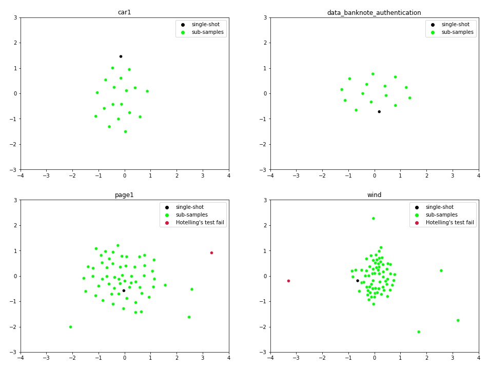
Figure 1: Low dimensional t-SNE visualization of the clustering indices estimated for the whole dataset population and dataset subsamples. The BLACK points represent the cluster indices of the whole dataset population, whereas the GREEN points represent cluster indices of the dataset subsamples. The RED points represent the subsamples that have failed Hotelling’s $T^{2}$ test.

We use Hotelling’s two-sample $T^{2}$ test [40], a multivariate extension of two-sample t-test for checking if a subsample is representative of the whole dataset population in terms of the respective dataset predictor variables. Figure 1 shows the subsamples that fail the Hotelling’s $T^{2}$ test (shown as RED dots) along with the passing subsamples (shown as GREEN dots). The subsamples that pass Hotelling’s test appear closer to the whole dataset population shown in BLACK color. A few subsamples appear relatively far from the entire population, but they seem to fail in Hotelling’s test appropriately. This observation confirms the agreement of Hotelling’s test response to the t-SNE visualization of the clustering indices.

One possible reason for some subsamples to go away from the whole population cluster indices is the randomness in sampling. The deviant subsamples are beneficial in the training phase as our dataset construction pipeline described in Section 3.3 considers each subsample as an independent dataset. Therefore, the far-away subsamples offer new dataset variance to our regressor $\mathcal{R}$ training that, in turn, should help the regressors to achieve better generalization over unseen datasets.

On the other hand, the deviant subsamples are problematic in the recommendation pipeline, as they might skew the estimated classification performance of the model classes in $\mathcal{C}$. Removing such deviant subsamples from the experiment requires the whole population cluster indices that might not be available at the testing time. To overcome this limitation, we propose to remove subsamples that fail the Hotelling’s $T^{2}$ test from the recommendation pipeline described in Section 3.4 to limit the skew due to random subsampling.

3.2 Automatic Model Selection System Architecture

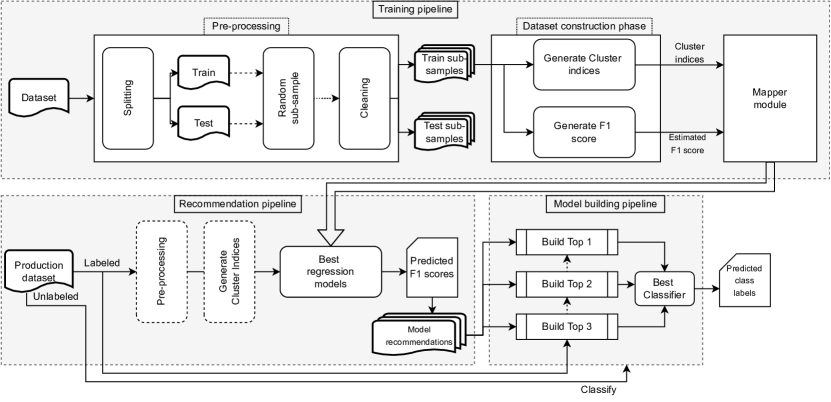
Figure 2: Architecture of the Automatic Model Selection System

The Automatic Model Selection system consists of two independent pipelines, one for training the underlying regression models and another pipeline for recommending the top-performing model classes for a given dataset. Figure 2 illustrates the overall architecture of the proposed automatic model selection system. The upper section is the Training pipeline, and the bottom is the model Recommendation pipeline. The Mapper module of the training pipeline contains the regressors for each model class that learn the mapping between clustering indices and model fitness. The model recommendation pipeline uses the learned regressors (Mapper modules) to predict the expected model fitness in terms of $F_{1}$ score (but not limited to) for each model class. The model classes that score the top3 $F_{1}$ scores become the best-fit classifier candidates for the given production dataset. We pick the best-performing classifier among the recommended top models through cross-validation to predict the labels of the unlabeled data.

3.3 Training Pipeline

The training phase has three subparts, namely:- A. Preprocessing, B) Data Construction, and C) Mappers as Regression models shown as the Training pipeline enclosed in the top dotted rectangle region in Figure 2.

Preprocessing:

Data preprocessing involves multiple sub-tasks to transform a single dataset $D_{i}$ into a set $\mathcal{B}_{i}$ of several subsamples generated by stratified random sampling with replacement. The dataset $D_{i}$ divides into 70:30 training-validation partitions for cross-validating the regressor model training. The training and validation partitions undergo random sampling independently to generate the respective subsamples. The constructed subsamples {$B_{ij}\}_{j=1}^{b}$ from a dataset $D_{i}$, undergo a cleansing process involving scaling and standardization. At the end of the preprocessing stage, we have a set $\mathcal{B}_{i}=\{B_{i1},B_{i2},\ldots,B_{ib}\}$ of several randomly sampled subsamples from both the training and validation partitions of the dataset $D_{i}$. The training process uses the training subsamples for learning and tuning the regressor functions $\mathcal{R}$ through cross-validation. We use the validation partitions for reporting the performance through $R^{2}$ score.

Model Class	Hyper-parameters
Logistic Regression	• Penalty: Elasticnet
Decision Tree	• Maxdepth: Tree grows until the leaves are pure, followed by backward-pruning for optimal depth • Criterion: Gini index
Regression Forest	• #Trees: 100 • Criterion: Gini index • Maxdepth: Tree grows until the leaves are pure, followed by backward-pruning for optimal depth
SVM	• Kernel: RBF • C (Penalty): Grid search over {0.01, 0.1, 1, 10, 100} • $\gamma$ (bandwidth) is set to $\frac{1}{p\times\sigma}$ – $\sigma$ is the variance of the flattened feature matrix $\mathbf{X}$ – $p$ is the data dimensionality
K-NN	• #Neighbors: Based on the Imbalance ratio (ex: K=R, if the ratio is 1:R)
XGBoost	• Maxdepth: Grid search over {1, 2, 4, 8, 16, 32, 64}

Table 2: Hyper-parameters for tuning the classifiers while estimating the model-fitness

Estimating model-fitness:

When applied to a dataset, the model-fitness score indicates what to expect as the classification performance from a model class. We set up the function $\mathcal{Q}(B;C)$ to measure the model-fitness of a classifier model class $C$ for the dataset $B$. We measure the model-fitness by estimating the maximum achievable classification performance measured using $F_{1}$ metric (but not limited to) by building tuned classifiers for the given dataset. Table 2 lists the tuning parameters we use for each model class to achieve optimal performance. We tune the classifiers for each of the given datasets to find the respective maximum achievable $F_{1}$ score and use the estimate as a surrogate measure for model-fitness. Our hyper-parameters list is not exhaustive but only indicative of the need for optimizing the model performance. We do this exercise through cross-validation to avoid an overfitting scenario that potentially skews the model-fitness score.

Data construction:

Given a set of subsamples $\mathcal{B}_{i}=\{B_{i1},B_{i2},\ldots,B_{ib}\}$ for training and validation drawn from each dataset $D_{i}\in\mathcal{D}$, the objective of the data construction phase is to generate a set of tuples $\{\langle\mathbf{I_{ij},O_{ij}}\rangle\}_{j=1}^{b}$ from all the subsamples in $\mathcal{B}_{i}$, where $\mathbf{I_{ij}}=\mathbb{F}(B_{ij})$ as per Eq. 1 and $\mathbf{O_{ij}}$ is the model-fitness score for a dataset $B_{ij}$ for every model class in $\mathcal{C}$ given by:

$$\mathbf{O_{ij}}\leftarrow\left[\mathcal{Q}(B_{ij};C_{1}),\mathcal{Q}(B_{ij};C_{2}),\ldots,\mathcal{Q}(B_{ij};C_{m})\right]^{T}$$ (4)

At the end of the data construction phase, we get a matrix of clustering indices feature vectors $\hat{\mathbf{I}}_{i}=[\mathbf{I}_{i1},\mathbf{I}_{i2},\ldots,\mathbf{I}_{ib}]^{T}$ generated for every subsample from the set $\mathcal{B}_{i}$ from dataset $D_{i}$ with the corresponding matrix of model-fitness scores $\hat{\mathbf{O}}_{i}=[\mathbf{O}_{i1},\mathbf{O}_{i2},\ldots,\mathbf{O}_{ib}]^{T}$ estimated for each model class in $\mathcal{C}$. Then, we combine the data generated for individual training datasets $D_{i}\in\mathcal{D}$ into a jumbo dataset $\langle\hat{\mathbf{I}},\hat{\mathbf{O}}\rangle$, such that:

$$\hat{\mathbf{I}}\leftarrow\left[\hat{\mathbf{I}}_{1},\hat{\mathbf{I}}_{2},\ldots,\hat{\mathbf{I}}_{N}\right]^{T}$$ (5)

$$\hat{\mathbf{O}}\leftarrow\left[\hat{\mathbf{O}}_{1},\hat{\mathbf{O}}_{2},\ldots,\hat{\mathbf{O}}_{N}\right]^{T}$$ (6)

Mapper for model selection:

In the Mapper phase, we learn a multiple regression function $\mathcal{R}:\hat{\mathbf{I}}\rightarrow\hat{\mathbf{O}}$ using the dataset $\langle\hat{\mathbf{I}},\hat{\mathbf{O}}\rangle$ generated from the Data Construction stage. We tune the hyper-parameter of the multiple regressors using the evaluation set through cross-validation. Alternately, instead of multiple regressors $\mathcal{R}$, we can also build individual regressors $R\in\mathcal{R}$ per model class $C\in\mathcal{C}$ as $R_{k}:\hat{\mathbf{I}}\rightarrow\hat{\mathbf{O}}^{(k)}$, where $\hat{\mathbf{O}}^{(k)}$ is the $k^{th}$ column-vector of the matrix $\hat{\mathbf{O}}$. The mapper module constitutes the resulting set of regressors $\mathcal{R}=\{R_{1},R_{2},\ldots,R_{m}\}$, which we use to predict the expected classification performance of different model classes $C_{k}\in\mathcal{C}$ for a given test dataset $D^{\prime}$.

During prediction, the mapper estimates the expected classification performance of a dataset from its clustering indices features. The expected classification performance is what an optimized/tuned classifier may achieve for a given dataset. We assume that the representation of the dataset samples in the clustering indices space follows the i.i.d assumption. This means that the parameter setting required for achieving higher performance for the training sample shall be similar to that of the validation sample. As the mapper learns to map the clustering indices to the tuned classifier performance during training, we expect the mapper to predict the closest estimate of optimized performance during validation.

3.4 Recommendation Pipeline

The automatic model selection system’s recommendation pipeline is a simple process of invoking the tuned regressor models $\mathcal{R}$ for predicting the expected model-fitness measured in terms of expected classification performance for a given test dataset $D^{\prime}$. The test dataset undergoes the same data transformation and cleansing stages as the training pipeline for consistency.

$$\mathbf{I}^{\prime}\leftarrow\mathbb{F}(D^{\prime})$$ (7)

The transformed data is input to each regressor function $R\in\mathcal{R}$ to predict the expected classification performance (model-fitness) score for all the model classes $C\in\mathcal{C}$.

$$\mathbf{O}^{\prime}\leftarrow\mathcal{R}(\mathbf{I}^{\prime})$$ (8)

We recommend the best model class $C_{best}$ that scores the highest model-fitness score for the given test dataset $D^{\prime}$.

$$i^{*}\leftarrow\arg\max_{\forall R_{i}\in\mathcal{R}}R_{i}(\mathbf{I}^{\prime})\equiv\arg\max_{1\leq i\leq m}\mathbf{O}^{\prime}_{i}$$ (9)

$$C_{best}\leftarrow C_{i^{*}}$$ (10)

Alternately, the prediction for the test dataset is also runnable using the data set subsamples, where we generate several subsamples $\mathcal{B}^{\prime}$ by random sampling with replacement from the input test dataset $D^{\prime}$ as $\mathcal{B}^{\prime}=\{B^{\prime}_{1},B^{\prime}_{2},\ldots,B^{\prime}_{b}\}$, where $B^{\prime}_{i}=\{d\ |\ d\sim D^{\prime}\}_{k=1}^{h},\forall B^{\prime}_{i}\in\mathcal{B}^{\prime}$. We then transform the subsamples to the clustering index feature space.

$$\mathbf{I}^{\prime}_{j}\leftarrow\left[\mathcal{F}_{1}(B^{\prime}_{j}),\mathcal{F}_{2}(B^{\prime}_{j}),\ldots,\mathcal{F}_{t}(B^{\prime}_{j})\right]^{T},\forall B^{\prime}_{j}\in\mathcal{B}^{\prime}$$ (11)

We input these vectors of cluster indices to the regressors $\mathcal{R}$ to make predictions of expected model-fitness scores for each of the model classes $C\in\mathcal{C}$.

$$\mathbf{O}^{\prime}_{j}\leftarrow\mathcal{R}(\mathbf{I}^{\prime}_{j}),1\leq j\leq b$$ (12)

We compute the expected model-fitness scores for all the model classes for the dataset $D^{\prime}$ by averaging the estimated fitness scores for each subsample $B^{\prime}\in\mathcal{B}^{\prime}$.

$$\mathbf{O}^{\prime}\leftarrow\frac{1}{b}\sum_{j=1}^{b}\mathbf{O}^{\prime}_{j}$$ (13)

With the availability of the estimated $F_{1}$ scores, the expected classification performance per model class from Equation 13, we use Equations 9 and 10 to recommend the best model class $C_{best}$ for the test dataset $D^{\prime}$.

Internal Indices	External Indices
Between-cluster scatter	Entropy
Banfeld-Raftery	Purity
Ball-Hall	Recall
PBM	Folkes-Mallows
Det-Ratio	Rogers-Tanimoto
Log-Det-Ratio	$F_{1}$
Ksq-DetW	Kulczynski
Score	Norm-Mutual-Info
Silhouette	Sokal-Sneath-1
Log-SS-Ratio	Rand
C-index	Hubert $\Gamma$
Dunn	Homogeneity
Ray-Turi	Completeness
Calinski-Harabasz	V-Measure
Trace-WiB	Jaccard
Davies-Bouldin	Adj-Rand
Within-cluster scatter	Phi
	McNemar
	Russel-Rao
	Precision
	Weighted-$F_{1}$
	Sokal-Sneath-2
	Adj-Mutual-Info

Table 3: Set of internal and external clustering indices $\mathcal{I}$

Model Class $\mathcal{C}$	Family	Clustering	Family
Decision Tree	Divisive	K-Means++	Convex
Logistic Regression	Linear	Agglomerative	Hierarchical
SVM	Large Margin	Spectral	Kernel, Non-convex
KNN	Lazy Learner	HDBSCAN	Density, Non-convex
Random Forest	Bagging Ensemble
XGBoost	Boosting Ensemble

Table 4: List of classifiers $C_{i}\in\mathcal{C}$ representing different model classes and the set of clustering methods $\mathcal{A}$ to generate clustering indices $\mathcal{I}$.

3.5 Configuration

The Automatic Model Section system requires configuration of the clustering indices set $\mathcal{I}$ and the list of representative model classes $\mathcal{C}$. Table 3 lists the set of clustering indices [41] that we configure the system to use for representing the dataset characteristics. The dataset clustering assumptions greatly influence the clustering indices. To make the clustering assumptions comprehensive, we configure multiple clustering algorithms representing different clustering assumptions on the dataset. Table 4 lists different clustering algorithms $A\in\mathcal{A}$ that we use to generate the respective clustering indices. We concatenate the clustering indices generated by these 4 (four) clustering methods to form a broader clustering index feature space of $4t$ dimensions.

$$\mathcal{I}=\left[\mathcal{I}_{A_{1}:kmeans},\mathcal{I}_{A_{2}:agglomerative},\mathcal{I}_{A_{3}:spectral},\mathcal{I}_{A_{4}:hdbscan}\right]$$ (14)

$$\mathcal{I}=\left[\underbrace{I_{1},I_{2},\ldots,I_{t}}_{A_{1}:kmeans},\underbrace{I_{t+1},I_{t+2},\ldots,I_{2t}}_{A_{2}:agglomerative},\underbrace{I_{2t+1},I_{2t+2},\ldots,I_{3t}}_{A_{3}:spectral},\underbrace{I_{3t+1},I_{3t+2},\ldots,I_{4t}}_{A_{4}:hdbscan}\right]$$ (15)

The transformation function set becomes $\mathbb{F}=\{\mathcal{F}_{1},\mathcal{F}_{2},\ldots,F_{4t}\}$ to cover the clustering indices from four different families of dataset clustering assumptions. We aim to use as many clustering indices as possible to build the dataset’s feature space representation. By scaling up the 40 (forty) dimensional clustering indices features from Table 3 with four different clustering algorithms from Table 4, we get a total of $4\times 40=160$ clustering indices features to represent the dataset characteristics. The mapper modules use an appropriate subset of the features while learning the association between clustering indices and the expected classification performance of a model class.

Dataset	Dims	Count	Dataset	Dims	Count
analcatdata_halloffame	17	1340	2d planes	10	40767
abalone	8	4176	contraceptive1_2	9	1473
balloon	2	2000	banana	2	5299
bank32nh	32	8192	car1	6	1728
chess	36	3196	churn	20	4999
cmc21	10	1473	coil2000	85	9822
connect4	43	67557	contraceptive1_1	9	1473
adult	14	48842	contraceptive1_3	9	1473
data_banknote_auth	5	1372	cpu_small	12	8192
flare	11	1066	default_of_credit	16	20000
credit_card_clients	20	1000	elevators	18	16599
fried	11	40768	hill valley	100	1211
HTRU_2	9	17898	image desert	136	2000
kdd_japaneseVowels	15	9961	kc1	21	2108
kin8nm	9	8190	kr-vs-kp	36	3196
magic04	10	19020	mushroom	22	5644
musk2	170	6598	mv	10	40768
optdigits	64	5620	page1	10	5472
pc1	21	1107	pendgits	16	10991
phoneme	6	5404	pizzacutter3	38	1043
pollen	6	3848	pol	48	15000
puma32H	33	8192	qsar_biodeg	42	1055
quake	4	2178	ring	20	7400
satimage1	36	6435	spambase	57	4597
splice1	60	3190	splice2	60	3190
splice3	60	3190	steel_plates	33	1940
tic-tac-toe	10	957	titanic	4	2200
tokyo	45	959	twonorm	20	7399
vehicle31	18	845	visualizing_soil	5	8641
wind	15	6574	waveform_5000	40	5000

Table 5: List of binary class datasets used for training and validating the proposed model selection

3.6 Classification Modeling As A Service

In an Automated ML setting, a user uploads a production dataset containing labeled and unlabeled parts to the service endpoint. The user then expects label predictions for the unlabeled part of the dataset without thinking about the underlying machine learning pipeline. As an enterprise extension to the Automatic Model Selection system, we expose the underlying data classification modeling as a service (an Automated ML SaaS offering) by abstracting the model selection, tuning, and training processes on a production dataset. Here, we rank the model classes by their estimated model fitness score and pick the best performing model among top3 models ($C_{A},C_{B},C_{C}\in\mathcal{C}$). We use the given labeled portion of the production dataset $\langle\mathbf{X},\mathbf{y}\rangle$ to cross-validate the top3 models with the best parameter settings. Using the best-performing model amongst the top3, we expose an API for predicting the class labels for the unlabeled portion of the production dataset. When the user invokes the API with the unlabeled data instance, the best-performing model among top3 classifiers outputs the class label $\hat{y}$ for the data instance $X$ from the test dataset $D^{\prime}$.

We describe the detailed validation of the end-to-end Automated ML system in Section 5.5 by comparing it against a few of the popular commercial and noncommercial Automated ML solutions.

4 Experimental setup

In this section, we test our Clustering Indices based Automatic classification Model Selection (CIAMS) hypothesis by cross-validating with several classification datasets collected from multiple public domain sources. We set up the experiment by choosing 6 (six) different classification model families listed in Table 4 representing various model classes.

4.1 Training Phase

We use sixty (60) binary class datasets in Table 5 to build our Automatic Model Selection system. We divide the datasets into train and test partitions. We use the train partition to build and tune our model selection system and the test partition to report the performance results. We divide train partition further into trainset and evalset partitions in a $k$-fold cross-validation setting to tune our model selection system. Each dataset from trainset and evalset partitions undergo sub-sampling independently. This ensures that we do not reuse any training data points during validation. Dataset subsampling increases the number of data points for training the mapper module (regressors) and exposes the underlying regressor models to more data variances. In total, we create 11,190 subsamples from all the $60$ datasets.

4.2 Evaluation Phase

We evaluate the performance of our Automatic Model Selection system using two modes, such as A) subsamples mode and B) single-shot mode. The subsamples mode mimics the dataset preparation strategy of the Training Phase, where we use only the subsamples of the datasets in the test partition for running the performance evaluation. Each dataset from the test partition gives out several test data points constructed from several subsamples drawn from it.

We set up cross-validation on 60 datasets using their respective subsamples. Traditionally, the sizes of the training and evaluation splits remain constant across all the cross-validation folds. In our setting, the split sizes vary proportionally to the population sizes of the datasets picked under the training and evaluation splits. We explain the proportionality in Section 4.3. We aim to construct the folds without any dataset spilling across folds. A fold may contain one or more datasets, but a dataset restricts to only one fold.

An ideal configuration to run the evaluation is Leave-One-(dataset)-Out. In our setting, the equivalent is running a $60$-fold cross-validation. We observe that 60-fold cross-validation on the subsamples of 60 datasets is time-consuming. To speed up, we repeat the 6-fold cross-validation exercise several times to approximate the results of 60-fold. Also, repeating the cross-validation several times allows us to test our method with different combinations of datasets in the training and testing folds.

On the contrary, we evaluate the single-shot mode through Leave-One-Out $60$-fold cross-validation. The single-shot mode uses the entire dataset from the test partition as one test record. The single-shot mode evaluation helps assess the system’s usefulness in enterprise deployment settings. An advantage of the subsamples mode is the ability to work with large datasets, as the full dataset single-shot approach might become resource-intensive for generating the clustering indices.

4.3 Hyper Parameters

A few hyperparameters control the system’s behavior, which we tune by trial and error.

Number of Clusters:

The number of clusters is a critical parameter for most clustering algorithms. We set the number-of-clusters parameter to $2$ for the clustering algorithms listed in Table 4. Initially, we allow a linear search for the number-of-cluster hyper-parameter. Our linear search experiment achieves the best results when the count is $2$.

Subsamples:

We set the subsample size as $h=500$ after doing a linear search with different subsample sizes when the size of the dataset $n$ is beyond 2000 points. We choose the following $h$-value for smaller datasets depending on the dataset size range.

$$h\leftarrow\left\{\begin{array}[]{lcl}100&\text{ }&n\leq 500\\ 300&\text{ }&500<n\leq 2000\\ 500&\text{ }&n>2000\\ \end{array}\right.$$

The number of subsamples $b$ is set proportional to the size of the dataset $n$. The average bootstrap subsample contains 63.2% of the original observations and omits 36.8% [42]. When the subsample size is $h$, we get $0.63h$ data points from the original dataset. The following equation helps us get the number of subsamples to draw from the dataset to ensure maximum coverage of dataset variances and more datasets for training our internal models. The hyper-parameter $\alpha$ is the oversampling constant, which we set to $5$ based on trial and error.

$$b\leftarrow\alpha\times\left\lceil\frac{n}{0.63h}\right\rceil$$

4.4 Scaling Up

Our present design of the CIAMS system uses four (4) clustering models on the datasets, six (6) classification model classes, and sixty (60) binary class datasets. We can train the underlying mapper module with more datasets $\mathcal{D}$ seamlessly to make the regressors robust for handling dataset variances. We can also add more model classes to $\mathcal{C}$ to increase the choices of classification methods for a given dataset. For comparison, the Azure AutoML platform uses about 12 classifiers from 8 model classes. Neural Networks and Bayesian methods are the two extra model classes other than the model classes listed in $\mathcal{C}$. Likewise, we can further expand the clustering indices feature space by adding other clustering methods to the set $\mathcal{A}$. The CIAMS system is scalable and extensible by design.

5 Evaluation

In this section, we evaluate the CIAMS system at different granularity levels in a bottom-up style to answer the following questions that may challenge our proposed scheme’s usefulness.

1. Is the dataset model-fitness a function of the dataset clustering indices for a model class?

2. Does the Mapper module implemented using Regression models efficiently learn the relationship between the dataset clustering indices and the expected classification performance of a selected model class?

3. What is the correctness of the recommendation given by the CIAMS system?

4. What is the performance of the end-to-end Classification Modeling as a Service platform for enterprise deployments?

5.1 Mapper Module Evaluation

Firstly, we evaluate the performance of the mapper module constructed using Regression models. Evaluating the regressors helps us understand the validity of our model selection hypothesis, which assumes that the clustering indices of a dataset strongly correlate with the expected classification performance of a chosen model class. We evaluate our idea using the estimated $R^{2}$ metric for every regressor built for every classifier model class. We also study the usefulness of the regressors through $L_{1}$-norm, or Mean Absolute Error (MAE) analysis between the predicted and actual dataset model-fitness measured using $F_{1}$ score. We run a small-sample statistical significance test on the $L_{1}$-norm estimates to check if the system contains the error margin within $\pm 10\%$.

Model Class	Single-shot	Subsamples
$C_{i}\in\mathcal{C}$	60-fold	6-fold
Decision Tree	0.83	0.81
Random Forest	0.89	0.86
Logistic Regression	0.87	0.84
K-Nearest Neighbor	0.80	0.80
XGBoost	0.85	0.83
SVM	0.81	0.81
Average	0.84	0.83

Table 6: Performance of the tuned Regressor functions $R_{i}\in\mathcal{R}$ for each model class $C_{i}\in\mathcal{C}$ measured using $R^{2}$ score in Single-Shot and Subsamples modes.

5.1.1 Regressor Performance

We designate a regressor $R_{i}$ for every classifier $C_{i}$ from the set of model classes $\mathcal{C}$. Each regressor function $R_{i}:\hat{\mathbf{I}}\rightarrow\hat{\mathbf{O}}^{(i)}$ learns a mapping between the cluster indices $\hat{\mathbf{I}}$ and the tuned classifier $C_{i}$ performance $\hat{\mathbf{O}}^{(i)}$ measured in $F_{1}$ metric for all the training datasets $\mathcal{D}$. We experiment with several regression models such as SVR, Random Forest, XGBoost, k-NN, and Decision Tree and select XGBoost to be the best regression model to learn the mapper through $R^{2}$ analysis. We train the regressor models using two configurations, namely:- A) single-shot, and B) subsamples mode as explained in Section 4.2. In the single-shot mode, we run Leave-One-(dataset)-Out cross-validation, and in the subsamples mode, we run $6$-fold cross-validation with six repeats to report the performance of the regressor models measured using $R^{2}$ score. We tune the XGBoost regressor models for best parameters by cross-validating on the train partition that gets split further into trainset and evalset partitions per fold. We repeat this exercise for all the classifiers in $\mathcal{C}$ to find the best XGBoost regression model parameters that maximize the $R^{2}$ score. Table 6 narrates the $R^{2}$ scores of the tuned regressors $R_{i}\in\mathcal{R}$; we build for every classifier $C_{i}\in\mathcal{C}$ in Single-Shot and Subsamples modes. We observe an average of 84% $R^{2}$ score for both modes, which confirms the feasibility of learning a mapping between clustering indices and model-fitness.

5.1.2 Prediction Correctness

We validate the regressors by checking if the predicted classification performance is similar to a model class’s expected classification performance on a dataset. We measure the similarity between the predicted and the expected classification performance measured as the model-fitness score ($F_{1}$) using Mean Absolute Error (MAE) or $L_{1}$-norm.

$$MAE\leftarrow\left\|F_{1}^{\;expected}-F_{1}^{\;predicted}\right\|$$ (16)

For every model class $C_{i}$, we consider the prediction of the mapper module (regressor $R_{i}$) to be a PASS if the absolute difference between the predicted and the actual classification performance is within 10% margin.

$$\texttt{Correctness}\leftarrow\left\{\begin{array}[]{lcl}\texttt{{PASS}}&\text{ }&\emph{MAE}\leq 10\%\\ \texttt{{FAIL}}&\text{ }&\emph{MAE}>10\%\end{array}\right.$$

Configuration	Single-shot (60-fold)		Subsamples (6-fold)
Model Class	#PASS	MAE	#PASS	MAE
Decision Tree	32	$0.14\pm 0.11$	38	$0.09\pm 0.05$
Random Forest	22	$0.13\pm 0.09$	46	$0.08\pm 0.04$
Logistic Regression	23	$0.17\pm 0.13$	37	$0.10\pm 0.07$
K-Nearest Neighbour	22	$0.13\pm 0.09$	31	$0.12\pm 0.08$
XGBoost	29	$0.11\pm 0.08$	46	$0.08\pm 0.05$
Support Vector Machine	23	$0.15\pm 0.11$	25	$0.13\pm 0.08$
Average	25		37

Table 7: Mapper module performance in terms of Prediction Correctness using MAE.

Table 7 summarizes the MAE and PASS performance of the mapper module. It is apparent from the table that the MAE is contained within $10\%$ for the majority of the datasets. In the Subsamples mode, the average MAE is slightly off for KNN, and SVM because of higher variance in the predicted $F_{1}$ scores. It is interesting to observe that the Mapping module achieves 10% compliance for over $75\%$ of the datasets for the ensembling methods with lower variance. The large-margin model class seems to have trouble with the stability in performance across different subsamples. An average of $37$ datasets have responded well to satisfy the $10\%$ error margin constraint. When the average MAE for a model class is within the $10\%$ margin, we are accurate in our prediction for over $61\%$ datasets. Ignoring the low-performing SVM classifier, the truncated average PASS performance stands at $40$, which is two-thirds of the datasets. The result of the subsampling mode is positively motivating to further this research avenue into achieving higher performance with better subsampling and model class tuning. On the other hand, in the Single-shot mode, the average MAE estimates are generally above the $10\%$ margin. Although the error margin is higher than $10\%$, the Mapper module makes accurate predictions for around $41\%$ of $60$ datasets. It is obvious from Table 7 that the Subsamples mode is more appropriate than the Single-shot mode for making predictions because the Mapper module inherently uses only the subsamples for training.

We perform the statistical significance test on the MAE estimate to check if the mapper module is indeed restricting the MAE within the 10% margin. We use the following version of the $t$ and $Z$-statistic [43] to perform the significance test. Suffixes $e$ and $p$ denotes the expected and predicted model-fitness ($F_{1}$) scores, $\Delta$ is the hypothesized difference between the population means $\bar{x}_{e},\bar{x}_{p}$ (we set $\Delta=0.1$).

$$Z\text{ or }t\text{-statistic}\rightarrow\frac{\left\|\bar{x}_{e}-\bar{x}_{p}\right\|-\Delta}{\sqrt{\frac{\sigma^{2}_{e}}{n_{e}}+\frac{\sigma^{2}_{p}}{n_{p}}}}$$ (17)

We run $t$-test when the number of samples is $\leq 30$, and $Z$-test when the sample count is $>30$ at $p=0.05$ significance. Table 8 summarizes the performance of the Mapper module tested against 60 datasets, where the second column lists the number of datasets where the MAE between expected and predicted model-fitness ($F_{1}$) score is within the $10\%$ margin at the statistical significance level of $p=0.05$. The $t/Z$-test confirms our regressors’ ability to accurately predict the expected classification performance for at least $60\%$ of the datasets.

Model Class	#PASS
Decision Tree	37
Random Forest	33
Logistic Regression	41
K-Nearest Neighbour	34
XGBoost	41
SVM	32
Average	36

Table 8: Performance evaluation of the Mapper module using two-sample $Z$-test & $t$-test in the Subsamples mode at $p=0.05$ significance

An average of above 60% PASS datasets in Tables 7 and 8 is interesting because, in the subsamples mode, we test the ability of the mappers to generalize on 10 unseen datasets per cross-validation fold. Out of 10 test-fold datasets, the mappers correctly predict the model-fitness for at least six datasets on average. A recall of 61% demonstrates excellent promise in the technique and increases the motivation to improve this idea further to achieve even higher recall. It is evident from the results in Tables 6, 7, and 8 that the Mapper module is efficient in learning the relationship between the clustering indices of a dataset and the expected classification performance of a model class. The results also empirically prove the validity of our hypothesis that the dataset model fitness is indeed a function of the dataset clustering indices for a model class.

5.2 Comparing Against Equivalent Methods

We argue that the clustering indices features represent the data characteristics. It is necessary to compare our approach against similar methods from the literature, such as Landmarking [34]. Landmarking determines the location of a specific learning problem in the space of all learning problems by measuring the performance of some simple and efficient learning algorithms. Landmarking attempts to characterize the data properties by building simple classifier models. Similarly, classic statistical and information-theoretic features directly represent the data characteristics. We compare the ability of the Landmarking and classic statistical, and information-theoretic features against clustering indices features to represent the data characteristics concerning a classification task.

Classic Statistical Features
Basic Statistics	Number of points Number of attributes Number of classes
Feature-based	F1- Maximum Fisher’s discriminant ratio F1v - Directional vector maximum Fisher’s discriminant ratio F2 - Volume of the overlapping region F3 - Maximum individual feature efficiency F4 - Collective feature efficiency
Neighborhood	N1 - Fraction of borderline points T1 - Fraction of hyper-spheres covering cardinality LSC - Local set average cardinality
Network	Density Hubs
Dimensionality	T2 - Average number of features per dimension T3 - Average number of PCA dimensions T4 - Ratio of PCA dimension to original dimension
Class Imbalance	C1 - Entropy of classes proportions C2 - Imbalance ratio
Landmarking Features
Linear	linear_discr - Score of Linear Discriminant classifier
Naive bayes	naive_bayes - Score of Naive Bayes classifier
Nearest Neighbour	elite_nn - Score of Elite Nearest Neighbor one_nn - Score of the 1-Nearest Neighbor classifier
Decision Tree	best_node - Score of the best single decision tree node random_node - Score of a single node model induced by a random attribute. worst_node - Score of a single node model induced by the worst attribute

Table 9: Statistical & Information-theoretic and Landmarking meta-features

There is no straightforward method to compare two data characteristics unless we use a downstream task to evaluate extrinsically. We describe our experiment below in steps, which compares the effectiveness of clustering indices against landmarking, statistical and information-theoretic features through the performance evaluation of an extrinsic regression task.

• Pick a subset of datasets from our experiment and frame a 5-fold cross-validation on the datasets

• Every dataset in the fold shall undergo subsampling individually

• Prepare the model-fitness scores (dependent variable) for each subsample

• Clustering Indices

  • Prepare the clustering indices (features) from Table 3 for each subsample

  • Learn regressors for each model class from clustering indices to model-fitness

• Classic Statistical Features

  • Collect a list of statistical & information-theoretic features [44, 45] as listed in Table 9

  • Generate the statistical features for each subsample

  • Learn regressors for each model class from statistical features to model-fitness

• Landmarking Features

  • Collect a list of landmarking features [46, 47] as listed in Table 9

  • Generate the landmarking features for each subsample

  • Learn regressors for each model class from landmarking features to model-fitness

• Measure the average cross-validation performance using $R^{2}$ score for the testing and training folds across model classes

	Clustering Indices		Statistical Features		Landmarking
Methods	Training	Testing	Training	Testing	Training	Testing
DT	0.90	0.89	0.75	0.57	0.61	0.48
RF	0.91	0.91	0.76	0.58	0.62	0.48
LR	0.89	0.89	0.77	0.61	0.62	0.59
KNN	0.90	0.89	0.75	0.59	0.61	0.44
XG	0.89	0.89	0.72	0.53	0.59	0.49
SVC	0.88	0.88	0.74	0.58	0.60	0.33
Mean	0.90	0.89	0.75	0.58	0.63	0.47

Table 10: Regressor $R^{2}$ performance comparison. The columns list the cross-validated training and testing performance of regressors when we use cluster indices, statistical & information-theoretic, and landmarking meta-features from the literature, respectively.

Table 10 summarizes the performance of the extrinsic regression task through i) clustering indices features, ii) classic statistical features, and iii) landmarking. It is apparent from the table that the clustering indices features are better than the other two strategies for capturing the dataset characteristics, at least with respect to an extrinsic regression task. The performance numbers show that the generalization error is higher for classic statistical features, although the training performance is reasonable. Landmarking, on the other hand, is unable to capture the dataset characteristics during training. As a result, the landmarking features generalize poorly during validation.

Choice of Clustering Indices				DT	RF	LR	KNN	SVC	XG
Internal Indices		External Indices		0.58	0.47	0.35	0.38	0.51	0.76
Internal Indices		External Indices		0.77	0.82	0.81	0.73	0.74	0.77
K-means	Hierarchical	Spectral	HDBSCAN	0.72	0.84	0.70	0.72	0.67	0.78
K-means	Hierarchical	Spectral	HDBSCAN	0.81	0.85	0.75	0.75	0.76	0.79
K-means	Hierarchical	Spectral	HDBSCAN	0.81	0.86	0.74	0.76	0.76	0.81
Kmeans	Hierarchical	Spectral	HDBSCAN	0.79	0.83	0.74	0.73	0.73	0.79
K-means	Hierarchical	Spectral	HDBSCAN	0.79	0.81	0.66	0.74	0.69	0.74
K-means	Hierarchical	Spectral	HDBSCAN	0.8	0.86	0.76	0.74	0.73	0.80
K-means	Hierarchical	Spectral	HDBSCAN	0.78	0.80	0.73	0.73	0.75	0.77
K-means	Hierarchical	Spectral	HDBSCAN	0.76	0.79	0.62	0.74	0.64	0.76
K-means	Hierarchical	Spectral	HDBSCAN	0.76	0.80	0.62	0.73	0.65	0.62
K-means	Hierarchical	Spectral	HDBSCAN	0.69	0.68	0.72	0.67	0.61	0.67
K-means	Hierarchical	Spectral	HDBSCAN	0.77	0.80	0.74	0.71	0.72	0.66
K-means	Hierarchical	Spectral	HDBSCAN	0.82	0.87	0.85	0.80	0.81	0.83

Table 11: Performance of the Mapper module for different configurations of clustering indices. Method indicates the ablation of the clustering indices from that specific clustering method while building the Mapper module. The Mapper model performs best when we use all clustering indices (internal & external) from all four families of clustering methods.

5.3 Ablation Study

Clustering indices reflect the ability of a clustering algorithm to form meaningful clusters over a dataset. A clustering algorithm may inherently suffer shortcomings due to its hypothesis and algorithmic limitations. For example, K-means cannot form nonconvex clusters, but methods such as Spectral clustering overcome this shortcoming. Likewise, Hierarchical clustering is very sensitive to outliers, but density-based methods such as HDBSCAN are resilient against outliers. This mentioned observation sets the premise for extracting clustering indices of a dataset using different clustering methods and concatenating them to create extended feature representation.

We perform our ablation study by dropping clustering indices from one or more specific clustering methods. We ablate the clustering indices to assess their relative contribution to an optimal build of the Mapper module. We also extend our ablation study to measure the contribution of internal vs. external cluster indices listed in Table 3. The performance of the Mapper module for different configurations of cluster indices is summarized in Table 11, where we observe that the Mapper model performs best when we use all the internal & external clustering indices from all four families of clustering methods.

Clustering index	Spearman Coefficient
C-index - Kmeans [48]	-0.40
Russel Rao - Spectral [49]	-0.51
Purity - Spectral [50]	-0.49
Entropy - Kmeans	0.35
Dunn - Hierarchical [51]	0.31
Silhouette - Spectral [52]	-0.46
Davies Bouldin - Spectral [53]	0.47
Precision - HDBSCAN	-0.43
Completeness - HDBSCAN [54]	0.51
PHI - Spectral [11]	0.28

Table 12: Top 10 critical features estimated using Spearman correlation score estimation between the clustering indices and the estimated classification performance on a dataset. The top features clearly indicate that they are spread across all the variations of clustering indices as analyzed by the Ablation study.

We further verify the result of the ablation study by observing the correlation between the feature importance and model-fitness. We extract the feature importance in terms of gain score [55] from the tree-based regressor (XGBoost) that learns the mapping between the clustering indices feature and the model-fitness. We analyze the correlation between the extracted high-gain cluster indices and the expected classification performance to estimate the magnitude and direction of the influence. Table 12 narrates the list of critical clustering indices (features) that influence the dataset model-fitness estimated using Spearman correlation measure. It is reassuring from the table that the critical features are distributed across all the variations of clustering indices, as suggested by the ablation study.

5.4 Evaluating End-to-End CIAMS System

We successfully validate our hypothesis that classification performance is a function of the dataset clustering indices for every model class by evaluating the performance of the Mapper module of CIAMS. We now study the end-to-end CIAMS system for the correctness of model-class recommendations given a test dataset. We use a $20-80$ train-test split to mimic the real-world production scenario where we get a limited labeled dataset to build models. This splitting also gives us an insight into the ability of the model to generalize with the availability of limited labeled data. As explained in Section 4.2, we validate the CIAMS system in both Single-shot and Subsamples mode. Given a test dataset $D^{\prime}$, we generate the feature vector $\mathbf{I}^{\prime}$ in the clustering indices feature space $\mathcal{I}$ using the procedure in Section 3.3 as $\mathbb{F}(D^{\prime};\mathcal{A}):D^{\prime}\rightarrow\mathbf{I}^{\prime}$. We supply the clustering indices feature vector $\mathbf{I}^{\prime}$ as input to regressors $R_{j}\in\mathcal{R}$ to predict the classification performance ${F_{1}}_{j}^{pred}$ as $\mathbf{O}^{\prime(j)}\leftarrow R_{j}(\mathbf{I}^{\prime};C_{j})$ for every model class $C_{j}$. In the subsampling mode, the resulting $F_{1}^{pred}$ scores are of dimension $b\times c$, where $b$ is the number of subsamples drawn from the dataset $D^{\prime}$ and $c$ is the number of model classes. In the Single-shot mode, the dimension is $1\times c$. The Subsamples model output is collapsed using Equation 13 into a $1\times c$ vector.

We now have the predicted model-fitness $F_{1}$ scores for the test dataset $D^{\prime}$ for each model class $C_{j}\in\mathcal{C}$. Sorting the model fitness $F_{1}$ scores in descending order gets us the ranked recommendation of suitable model classes for the given test dataset $D^{\prime}$. We call the top3 model classes as $C_{A}^{pred},C_{B}^{pred},C_{C}^{pred}$ in the higher to lower classification performance order ($C_{A}\geq C_{B}\geq C_{C}$). We compare the predicted rank order $C_{A}^{pred},C_{B}^{pred},C_{C}^{pred}$ with the true rank order $C_{A}^{true},C_{B}^{true},C_{C}^{true}$. To get the “true” rank order of the model classes, we build tuned classifier models for all the model classes using the same dataset $D^{\prime}$ that we feed to the Recommendation pipeline. We tune all the classification models through cross-validation. We use the evaluation score for the model classes to rank-order the classifiers, which in turn yields us $C_{A}^{true},C_{B}^{true},C_{C}^{true}$.

5.4.1 Validation

We validate the performance of CIAMS using the corpus of 60 datasets. Table 13 presents the confusion matrix of the predicted and actual top3 model class recommendation by the CIAMS system in both the Single-shot and Subsampling modes. Although the ranks are not exact matches, we observe a strong overlap between the true and the predicted top3 model classes. From the table, we observe that CIAMS can recall (highlighted in YELLOW) the true top1 model class among the predicted top3 model class with recall scores of 78% and 74% in the Single-shot and Sub-sampling modes respectively. Likewise, the top1 prediction from CIAMS can recall the true top3 model classes with recall scores of 74% and 70% in the Single-shot and Sub-sampling modes, respectively. The ability to recall the top1 model class in three-fourths of the test datasets is remarkable.

	Single-shot (60-fold)					Subsamples (6-fold $\times$6)
	$\ C_{A}^{pred}$	$\ C_{B}^{pred}$	$\ C_{C}^{pred}\$	Total	Hit	$\ C_{A}^{pred}$	$\ C_{B}^{pred}$	$C_{C}^{pred}\$	Total	Hit
$C_{A}^{true}$	19	16	12	47	78%	157	68	41	266	74%
$C_{B}^{true}$	12	10	12	34	55%	66	73	82	221	61%
$C_{C}^{true}$	13	9	8	30	50%	28	66	58	152	42%
Total	44	35	32	60		251	207	181	362
Hit	74%	58%	53%			70%	58%	50%

Table 13: Confusion matrix of the true and predicted top3 model classes in Single-shot and Subsampling modes.

Dataset	Dims	Count	$C_{A}^{pred}$	$C_{B}^{pred}$	$C_{C}^{pred}$	$C_{voting}^{pred}$
australian	15	689	0.61	0.84	0.83	0.83
bankruptcy	7	250	0.51	0.97	0.96	0.92
christine	1637	5417	0.65	0.71	0.70	0.70
cleve	14	302	0.68	0.66	0.78	0.77
haberman	4	305	0.32	0.35	0.43	0.52
jm1	22	10879	0.42	0.51	0.50	0.46
mfeat-morphological	7	1999	0.70	0.82	0.99	0.98
monk-2	7	431	0.80	0.98	0.98	0.98
nba_logreg	20	1328	0.66	0.65	0.60	0.63
no2	8	499	0.54	0.55	0.56	0.56
ozone	73	2533	0.37	0.42	0.31	0.43
philippine	309	5831	0.72	0.68	0.66	0.73
phisingwbsite	31	11054	0.92	0.92	0.95	0.95
piechart3	38	1076	0.34	0.46	0.20	0.37
saheart	10	461	0.58	0.58	0.60	0.60
scene_urban	300	2406	0.95	0.90	0.97	0.95
segment	20	2309	0.97	0.98	0.97	0.98
speech	401	3685	0.34	0.46	0.20	0.37
UniversalBank	13	4999	0.41	0.51	0.48	0.48
wine4	12	1598	0.12	0.03	0.13	0.12
amazon_emp_access*	9	32769	0.05	0.18	0.26	0.11
clickpred_small*	12	39948	0.15	0.43	0.41	0.42
namoa*	120	34465	0.94	0.91	0.92	0.93
FOREX_eurgbp*	11	43825	0.49	0.37	0.50	0.50
run_or_walk_info*	8	88588	0.98	0.98	0.99	0.98

Table 14: Performance comparison of the top3 classifiers recommended by CIAMS. The best overall score is bold-faced and underlined. The second-best score is in italics. The performance of the Weighted Voting Classifier is higher than the top3 classifiers in three highlighted datasets.

5.4.2 Testing

We test CIAMS’s top3 recommend model classes using a separate hold-out set of public domain binary class datasets listed in the first column of Table 14. We compare the actual classification performance of the top3 model classes and tabulate the results in Table 14. We report the 5-fold cross-validation performance of the top3 classifiers on the test datasets. The top3 recommended classifiers win in 22 of 25 datasets. By running cross-validation, we use the best of top3 recommended classifiers for a given test dataset. Essentially, we bring the complexity down from running an exhaustive model search to choosing the best from only three choices. We use the best classifier from the recommended list as the underlying model of the end-to-end Automated ML system to expose a SaaS API for automatic dataset classification.

As an exercise, we also ensemble the top3 classifiers into a Weighted Voting Classifier ${C}_{voting}$. We list the ensemble’s performance in the last column of Table 14. The voting classifier works best for 9 of 25 datasets. When we consider the top2 scores from the column, we find that the voting classifier performs well for 21 of 25 datasets. The voting classifier abstracts the top3 models, simplifying the Automated ML pipeline with one final prediction model. Of the 9 (nine) best scores, we also observe that the voting classifier ensemble is marginally better than the constituent classifiers in 3 (three) datasets highlighted in YELLOW in Table 14. As the performance improvement is not significant, we choose to skip ensembling the top3 model classes.

5.5 Validating CIAMS based end-to-end Automated ML System

Automated Machine Learning platforms provide significant cost savings to businesses, focusing on complex processes such as product innovation, market penetration, and enhanced client satisfaction. Automated ML platforms decrease the energy spent on time and resource-consuming processes such as model selection, feature engineering, and hyper-parameter tuning. The major cloud players such as Microsoft and Amazon have their version of the Automated ML platforms. In responding to the demand for accessible and affordable automatic machine learning platforms, open-source frameworks are also available to put the data to use as quickly and with as little effort as possible. Table 15 lists a limited set of commercial and open-source Automated ML platforms, with which we make a performance comparison against CIAMS based Automated ML system.

Automated ML Platform	Name
Auto-sklearn	A-SKL
Auto-WEKA	A-Weka
TPOT	TPOT
Microsoft Azure Automated ML	Azure
Amazon SageMaker	SageMaker
H2O AutoML	H2O
FLAML	FLAML

Table 15: A limited list of commercial and open-source Automated ML platforms.

Automated machine learning frameworks generally apply standardized techniques for feature selection, feature transformation, and data imputation on datasets developed over the years. However, the underlying methods used to automate machine learning tasks are different. We experimentally assess these methods in an end-to-end style across various datasets. We perform a quantitative comparison of the performance of CIAMS measured using $F_{1}$ score with the other Automated ML candidate methods listed in Table 15.

Commercial and noncommercial Automated ML platforms apply different model ensembling techniques to boost performance. In our design, we use the top3 CIAMS recommended model classes and build the classifiers using the labeled part of the Production dataset and tune the constituent classifiers using $5$-fold cross-validation. We compare the evaluation (or test) set performance of the best-performing model among the top3 CIAMS against the performance of the other Automated ML methods in Table 16.

Dataset	CIAMS	FLAML	H2O	TPOT	A-WEKA	AzureML	SageMaker	A-SKL
australian	0.84	0.84	0.85	0.84	0.82	0.87	-	0.85
bankruptcy	0.97	0.98	0.97	0.94	0.91	-	-	0.75
christine	0.71	0.68	0.71	0.70	0.65	0.70	0.68	0.70
cleve	0.78	0.70	0.77	0.78	0.68	0.27	-	0.75
haberman	0.43	0.38	0.40	0.55	0.47	0.26	-	0.32
jm1	0.51	0.36	0.50	0.45	0.43	0.37	0.55	0.22
mfeat-morphological	0.99	0.99	0.99	0.99	0.99	0.99	-	0.99
monk-2	0.98	0.99	0.98	0.98	1.00	0.99	-	1.00
nba_logreg	0.66	0.57	0.62	0.65	0.67	0.67	-	0.65
no2	0.56	0.58	0.50	0.56	0.55	0.58	-	0.58
ozone	0.42	0.29	0.42	0.37	0.37	0.20	0.43	0.40
philippine	0.72	0.73	0.68	0.73	0.58	0.73	0.71	0.72
phisingwbsite	0.95	0.95	0.96	0.94	0.94	0.96	0.93	0.95
piechart3	0.46	0.31	0.27	0.39	0.30	0.23	-	0.36
saheart	0.60	0.60	0.60	0.57	0.56	0.59	-	0.62
scene_urban	0.97	0.92	0.56	0.97	0.33	0.91	-	0.97
segment	0.98	0.98	0.98	0.98	0.96	0.99	-	0.99
speech	0.46	0.02	0.27	0.39	0.04	0.02	0.15	0.36
UniversalBank	0.51	0.47	0.49	0.49	0.43	0.45	0.36	0.45
wine4	0.13	0.06	0.03	0.03	0.06	0.03	-	0.13
amazon_emp_access*	0.26	0.05	0.23	0.22	0.15	0.15	0.37	0.26
clickpred_small*	0.43	0.15	0.44	0.37	0.21	0.16	-	0.22
namao*	0.94	0.21	0.94	0.93	0.92	0.94	0.91	0.93
FOREX_eurgbp*	0.50	0.34	0.45	0.50	0.50	0.50	-	0.51
run_or_walk_info*	0.99	0.34	0.98	0.98	0.95	0.98	-	0.98
#Top1 Performance	10	4	5	5	3	8	3	8
#Top2 Performance	22	10	12	14	5	5	3	15
#Top3 Performance	25	12	17	21	11	15	4	20
Average Rank	1.68	3.36	2.64	2.4	3.64	3.3	3.11	2.56

Table 16: Weighted $F_{1}$ score achieved by different Automated ML methods for various public domain binary class datasets (as production datasets) in the Single-shot setting. The best score is presented as underlined & bold-faced, the second best is bold-faced and the next best is italicized. The average rank is the average of the rank order position scored by each Automated ML method, where a low number means higher-performance. Datasets with a * marker are larger in size.

While comparing the performance of CIAMS against other Automated ML methods, we provide the test dataset in full as input to all the systems evaluated in this experiment. We observe from Table 16 that CIAMS is winning against the other methods with an average rank of 1.68, followed by Auto-weka scoring an average of 2.4. It is interesting to observe the CIAMS method scoring a definite top3 position in all 25 test datasets. The clear win also reflects in the number of top2 positions at 22 of 25. This observation gives us a strong validation that CIAMS based end-to-end Automated ML system is at par if not better than other commercial and open-source automated machine learning methods even without any explicit feature engineering incorporated by the other methods.

Dataset	FLAML	H2O	TPOT	A-WEKA	A-SKL
australian	WIN	WIN	LOSE	WIN	WIN
bankruptcy	WIN	WIN	WIN	WIN	WIN
christine	WIN	WIN	WIN	WIN	LOSE
cleve	LOSE	LOSE	LOSE	WIN	LOSE
haberman	WIN	WIN	LOSE	WIN	WIN
jm1	WIN	LOSE	WIN	WIN	WIN
mfeat-morphological	WIN	LOSE	LOSE	WIN	WIN
monk-2	WIN	WIN	WIN	WIN	LOSE
nba_logreg	WIN	WIN	WIN	WIN	WIN
no2	WIN	WIN	WIN	WIN	WIN
ozone	WIN	LOSE	LOSE	WIN	WIN
philippine	WIN	WIN	WIN	WIN	WIN
phisingwbsite	WIN	WIN	WIN	WIN	LOSE
piechart3	WIN	WIN	WIN	WIN	WIN
saheart	WIN	LOSE	LOSE	WIN	LOSE
scene_urban	WIN	WIN	WIN	WIN	WIN
segment	WIN	WIN	WIN	WIN	WIN
speech	WIN	LOSE	WIN	WIN	WIN
UniversalBank	WIN	WIN	WIN	-	WIN
wine4	WIN	LOSE	LOSE	WIN	WIN
amazon_emp_access*	WIN	WIN	WIN	WIN	WIN
clickpred_small*	WIN	LOSE	LOSE	WIN	WIN
namao*	LOSE	LOSE	WIN	WIN	LOSE
FOREX_eurgbp*	WIN	WIN	LOSE	WIN	LOSE
run_or_walk_info*	WIN	WIN	WIN	-	WIN
						AVG
WIN %	92%	64%	64%	100%	72%	78.4%
LOSE %	8%	36%	36%	0%	28%	21.6%

Table 17: Student’s $t$-test results with a significance level of $0.02$ for the comparison of CIAMS against other Automated ML methods.

.

We further study the statistical significance of the performance of CIAMS against other Automated ML methods using two samples $t$-test in Table 17. It is evident from the table that CIAMS wins over the other methods in an average of three-fourths (78%) of the test datasets. The next best methods in the comparison are TPOT and H2O, where CIAMS wins in two-thirds (64%) of the test datasets population. It is remarkable to observe CIAMS ruling over FLAML, and Auto-WEKA with 92% and 100% wins. From Tables 16 and 17, we conclude that CIAMS is a great contender for becoming an Automated ML system for dataset classification in production settings.

Dataset	CIAMS	FLAML	H20	TPOT	A-WEKA	AzureML	SageMaker	A-SKL
australian	10.9	11.1	13.8	30.5	184.0	1064.6	-	3745.3
bankruptcy	9.2	9.4	34.3	30.0	197.0	-	-	4699.3
christine	586.8	606.9	1181.7	209.6	290.0	1273.4	2832.7	3705.9
cleve	9.7	9.9	101.9	65.8	196.0	1111.5	-	4699.3
haberman	16.3	16.6	18.2	28.8	206.0	1089.3	-	3668.3
jm1	388.8	3120.5	35.2	157.2	178.0	1110.2	1835.7	3605.0
mfeat-morphological	20.9	21.1	34.5	33.2	171.0	1102.0	-	3644.9
monk-2	9.3	9.4	24.6	24.0	169.0	1128.1	-	3811.9
nba_logreg	19.1	19.2	14.2	29.1	165.0	1156.2	-	3664.9
no2	9.8	10.0	19.0	35.0	173.0	1117.0	-	3641.8
ozone	71.5	71.9	51.5	70.3	212.0	1152.9	1805.6	3620.4
philippine	534.4	536.1	156.4	358.9	202.0	1179.3	1986.9	3604.5
phisingwbsite	367.0	3224.0	45.3	67.9	417.0	1131.8	1745.4	3621.4
piechart3	24.4	24.7	20.1	25.3	180.0	1141.4	-	3706.5
saheart	15.6	15.7	16.8	30.7	184.0	1133.5	-	3716.7
scene_urban	93.4	94.0	111.4	210.2	180.0	1165.7	-	3618.7
segment	32.0	32.3	68.4	29.5	158.0	1092.4	-	3741.8
speech	24.4	25.3	20.1	25.3	197.0	1170.7	2168.1	3706.5
UniversalBank	268.6	268.7	19.2	64.9	170.0	1154.1	1835.7	3611.9
wine4	18.0	18.2	19.3	26.3	188.0	1161.3	-	7188.5
amazon_emp_access*	340.7	341.1	53.0	86.7	171.9	1150.9	2046.8	3624.7
clickpred_small*	278.3	279.2	53.7	63.7	5139.0	1131.4	-	3614.6
namao*	649.7	651.4	528.7	124.9	325.0	1137.7	2077.5	3737.3
FOREX_eurgbp*	403.7	515.7	50.8	117.7	205.0	1112.8	-	3754.0
run_or_walk_info*	615.2	403.9	188.0	83.4	13920.0	1145.4	-	3648.7
#Fastest Performance	12	0	9	4	0	0	0	0
#Faster Performance	14	12	11	10	3	0	0	0

Table 18: Comparison of time taken (in seconds) by CIAMS and other Automated ML methods for different binary class datasets. The shortest time is presented as underlined & bold-faced and the second shortest is bold-faced. Datasets with a * marker are larger in size.

Table 18 shows the time taken by each of the automated machine learning methods for building models and making predictions, end-to-end. Amazon SageMaker and Auto-sklearn are the slowest methods consuming over an hour for each dataset. Azure Automated ML is the next slowest method, consuming over 15 mins for each dataset on average. TPOT is reasonably faster, with an average time of less than a minute. FLAML and H2O AutoML are the second fastest methods to make CIAMS the fastest method for automated machine learning in a limited dataset experiment. CIAMS scores the top1 fastest position on 12 and top2 faster position on 14 datasets out of 25.

6 Conclusion

CIAMS is a scalable and extensible method for automatic model selection using the clustering indices estimated for a given dataset. We build an end-to-end pipeline for recommending the best classification model class for a given production dataset based on the dataset’s characteristics as represented in the clustering index feature space. Our experimental setup with 60 different binary class datasets confirms the validity of our hypothesis that the classification performance of a dataset is a function of the dataset clustering indices with $R^{2}>80\%$ score for all the model classes included in the setup. We also observe that our mapper module predicts the expected classification performance within 10% error margin for an average of two-thirds of 60 datasets in the subsampling mode. While evaluating the rank-order prediction, we observe that our automatic model selection method scores precise top3 predictions for three-fourths of 60 datasets. We also develop an end-to-end automatic machine learning system for data classification. A user can send a test dataset and acquire the classification labels without worrying about the classification model selection and building processes. When we compare against popular commercial and open-source automatic machine learning platforms with another set of 25 binary class datasets, we outperform others with an average rank of 1.68 in classification performance, even in the absence of the explicit feature engineering performed by other platforms. Regarding running time, we show that CIAMS is significantly faster than the other methods. The next step for CIAMS is to extend the platform for multi-class classification and regression tasks to make it a complete Automated ML suite. The codebase for this work is available in Github.

7 Data Availability

The datasets generated during and/or analyzed during the current study are available from the corresponding author upon reasonable request.

8 Acknowledgment

This work was supported by Claritrics Inc. d.b.a BUDDI AI under Grant number RB1920CS200BUDD008156. On behalf of all authors, the corresponding author states that there is no conflict of interest.

References

- [1] Pavel B. Brazdil, Carlos Soares, and Joaquim Pinto da Costa. Ranking learning algorithms: Using IBL and meta-learning on accuracy and time results. Machine Learning, 50(3):251–277, 2003.
- [2] Roman Vainshtein, Asnat Greenstein-Messica, Gilad Katz, Bracha Shapira, and Lior Rokach. A hybrid approach for automatic model recommendation. In CIKM ’18, 2018.
- [3] Noy Cohen-Shapira, Lior Rokach, Bracha Shapira, Gilad Katz, and Roman Vainshtein. Autogrd: Model recommendation through graphical dataset representation. In Proceedings of the 28th ACM International Conference on Information and Knowledge Management, CIKM ’19, page 821–830, New York, NY, USA, 2019. Association for Computing Machinery.
- [4] Iddo Drori, Yamuna Krishnamurthy, Raoni Lourenço, Rémi Rampin, Kyunghyun Cho, Cláudio T. Silva, and Juliana Freire. Automatic machine learning by pipeline synthesis using model-based reinforcement learning and a grammar. CoRR, abs/1905.10345, 2019.
- [5] Chris Thornton, Frank Hutter, Holger H Hoos, and Kevin Leyton-Brown. Auto-weka: Combined selection and hyperparameter optimization of classification algorithms. In Proceedings of the 19th ACM SIGKDD international conference on Knowledge discovery and data mining, pages 847–855. ACM, 2013.
- [6] Matthias Feurer, Aaron Klein, Katharina Eggensperger, Jost Springenberg, Manuel Blum, and Frank Hutter. Efficient and robust automated machine learning. In C. Cortes, N. D. Lawrence, D. D. Lee, M. Sugiyama, and R. Garnett, editors, Advances in Neural Information Processing Systems 28, pages 2962–2970. Curran Associates, Inc., 2015.
- [7] Randal Olson and Jason Moore. TPOT: A Tree-Based Pipeline Optimization Tool for Automating Machine Learning, pages 151–160. JMLR, 05 2019.
- [8] Boyuan Chen, Harvey Wu, Warren Mo, Ishanu Chattopadhyay, and Hod Lipson. Autostacker: A compositional evolutionary learning system. CoRR, abs/1803.00684, 2018.
- [9] Esteban Real, Chen Liang, David R. So, and Quoc V. Le. Automl-zero: Evolving machine learning algorithms from scratch. ArXiv, abs/2003.03384, 2020.
- [10] Lisha Li, Kevin G. Jamieson, Giulia DeSalvo, Afshin Rostamizadeh, and Ameet Talwalkar. Efficient hyperparameter optimization and infinitely many armed bandits. ArXiv, abs/1603.06560, 2017.
- [11] Martin Maechler, Peter Rousseeuw, Anja Struyf, Mia Hubert, and Kurt Hornik. cluster: Cluster analysis basics and extensions. The Comprehensive R Archive Network, 2019. R package version 2.0.8.
- [12] Tin Kam Ho. A data complexity analysis of comparative advantages of decision forest constructors. Pattern Analysis & Applications, 5(2):102–112, Jun 2002.
- [13] Piali Das, Valerio Perrone, Nikita Ivkin, Tanya Bansal, Zohar Karnin, Huibin Shen, Iaroslav Shcherbatyi, Yotam Elor, Wilton Wu, Aida Zolic, Thibaut Lienart, Alex Tang, Amr Ahmed, Jean Baptiste Faddoul, Rodolphe Jenatton, Fela Winkelmolen, Philip Gautier, Leo Dirac, Andre Perunicic, Miroslav Miladinovic, Giovanni Zappella, Cédric Archambeau, Matthias Seeger, Bhaskar Dutt, and Laurence Rouesnel. Amazon sagemaker autopilot: a white box automl solution at scale, 2020.
- [14] Abishek Mishra. Amazon SageMaker, chapter 16, pages 353–385. John Wiley & Sons, Ltd, 2019.
- [15] Erin LeDell and Sebastien Poirier. H2O AutoML: Scalable automatic machine learning. 7th ICML Workshop on Automated Machine Learning (AutoML), July 2020.
- [16] H2O.ai. H2O AutoML, June 2017. H2O version 3.30.0.1.
- [17] D. Mukunthu, P. Shah, and W.H. Tok. Practical Automated Machine Learning on Azure: Using Azure Machine Learning to Quickly Build AI Solutions. O’Reilly Media, Incorporated, 2019.
- [18] Nicolo Fusi, Rishit Sheth, and Melih Huseyn Elibol. Probabilistic matrix factorization for automated machine learning. In NIPS 2018. arXiv:1705.-5355v2, December 2018. Preprint posted to Cornell University Library.
- [19] Chi Wang, Qingyun Wu, Markus Weimer, and Erkang Zhu. Flaml: A fast and lightweight automl library. In MLSys, 2021.
- [20] Pavel B. Brazdil and Carlos Soares. Ranking classification algorithms based on relevant performance information. In MetaLearning: Building Automatic Advice Strategies for Model Selection and Method Combination, 2000, 2000.
- [21] Yannis Poulakis, Christos Doulkeridis, and Dimosthenis Kyriazis. A framework for automated clustering based on cluster validity indices. Proceedings of the 20th IEEE International Conference on Data Mining, 2020.
- [22] Deep Sahni, Satya Jayadev Pappu, and Nirav Bhatt. Aided selection of sampling methods for imbalanced data classification. In 8th ACM IKDD CODS and 26th COMAD, CODS COMAD 2021, page 198–202, New York, NY, USA, 2021. Association for Computing Machinery.
- [23] Sudarsun Santhiappan, Nitin Shravan, and Balaraman Ravindran. Is it hard to learn a classifier on this dataset? In 8th ACM IKDD CODS and 26th COMAD, CODS COMAD 2021, page 299–306, New York, NY, USA, 2021. Association for Computing Machinery.
- [24] Gilad Katz, Eui Chul Richard Shin, and Dawn Xiaodong Song. Explorekit: Automatic feature generation and selection. 2016 IEEE 16th International Conference on Data Mining (ICDM), pages 979–984, 2016.
- [25] Robert Engels and Christiane Theusinger. Using a data metric for preprocessing advice for data mining applications. In In Proceedings of the European Conference on Artificial Intelligence (ECAI-98, pages 430–434. John Wiley & Sons, 1998.
- [26] Ling Li and Yaser Abu-mostafa. Data complexity in machine learning. Caltech Computer Science Technical Report, 2006.
- [27] A Orriols-Puig, Núria Macià, and Tin Ho. Dcol: Data complexity library in c++ (documentation), 01 2010.
- [28] Ramón A. Mollineda, J. Salvador Sánchez, and José M. Sotoca. Data characterization for effective prototype selection. In Jorge S. Marques, Nicolás Pérez de la Blanca, and Pedro Pina, editors, Pattern Recognition and Image Analysis, pages 27–34, Berlin, Heidelberg, 2005. Springer Berlin Heidelberg.
- [29] Yonghong Peng, Peter A. Flach, Carlos Soares, and Pavel Brazdil. Improved dataset characterisation for meta-learning. In Proceedings of the 5th International Conference on Discovery Science, DS ’02, page 141–152, Berlin, Heidelberg, 2002. Springer-Verlag.
- [30] Hilan Bensusan. Odd bites into bananas don”t make you blind: Learning about simplicity and attribute addition. Technical report, University of Bristol, GBR, 1998.
- [31] Hilan Bensusan, Christophe Giraud-Carrier, and Claire Kennedy. A higher-order approach to meta-learning. Technical report, University of Bristol, GBR, 2000.
- [32] Aarnoud Hoekstra and Robert P. W. Duin. On the nonlinearity of pattern classifiers. Proceedings of 13th International Conference on Pattern Recognition, 4:271–275 vol.4, 1996.
- [33] Hilan Bensusan and Christophe Giraud-Carrier. Discovering task neighbourhoods through landmark learning performances. Proceedings of the Fourth European Conference on Principles and Practice of Knowledge Discovery in Databases, pages 325–330, 01 2000.
- [34] Bernhard Pfahringer. Meta-learning by landmarking various learning algorithms. Proceedings of the Seventeenth International Conference on Machine Learning, 05 2001.
- [35] Johannes Fürnkranz and Johann Petrak. An evaluation of landmarking variants. In C. Giraud-Carrier, Nada Lavrac, Steve Moyle, and B. Kavsek, editors, Proceedings of the ECML/PKDD Workshop on Integrating Aspects of Data Mining, Decision Support and Meta-Learning (IDDM-2001), pages 57–68, 2001.
- [36] Johann Petrak. Fast subsampling performance estimates for classification algorithm selection. In Proceedings of the ECML-00 Workshop on Meta-Learning: Building Automatic Advice Strategies for Model Selection and Method Combination, pages 3–14, 2000.
- [37] Luís Paulo Garcia, Andre de Carvalho, and Ana Lorena. Effect of label noise in the complexity of classification problems. Neurocomputing, 160, 02 2015.
- [38] Gleison Morais and Ronaldo Prati. Complex network measures for data set characterization. In Complex Network Measures for Data Set Characterization, pages 12–18, 10 2013.
- [39] Laurens van der Maaten and Geoffrey Hinton. Viualizing data using t-sne. Journal of Machine Learning Research, 9:2579–2605, 11 2008.
- [40] Harold Hotelling. The Generalization of Student’s Ratio. The Annals of Mathematical Statistics, 2(3):360 – 378, 1931.
- [41] Bernard Desgraupes. Clustering indices. Technical report, The Comprehensive R Archive Network, 2013.
- [42] Michael R. Chernick and Robert A. LaBudde. An Introduction to Bootstrap Methods with Applications to R. Wiley Publishing, 1st edition, 2011.
- [43] Allan G. Bluman. Elementary statistics: a step by step approach. McGraw-Hill, 2012.
- [44] Ana Lorena, Luís Paulo Garcia, Jens Lehmann, Marcilio de Souto, and Tin Ho. How complex is your classification problem?: A survey on measuring classification complexity. ACM Computing Surveys, 52:1–34, 09 2019.
- [45] Joanna Komorniczak and Pawel Ksieniewicz. problexity – an open-source python library for binary classification problem complexity assessment, 2022.
- [46] Edesio Alcobaça, Felipe Siqueira, Adriano Rivolli, Luís P. F. Garcia, Jefferson T. Oliva, and André C. P. L. F. de Carvalho. Mfe: Towards reproducible meta-feature extraction. Journal of Machine Learning Research, 21(111):1–5, 2020.
- [47] Edesio Alcobaça, Felipe Siqueira, Adriano Rivolli, Luís P. F. Garcia, Jefferson T. Oliva, and André C. P. L. F. de Carvalho. pymfe: Python meta-feature extractor.
- [48] Lawrence Hubert and James Schultz. Quadratic assignment as a general data analysis strategy. British Journal of Mathematical and Statistical Psychology, 29(2):190–241, 1976.
- [49] C. Radhakrishna Rao. The utilization of multiple measurements in problems of biological classification. Journal of the Royal Statistical Society: Series B (Methodological), 10(2):159–193, 1948.
- [50] Christopher D. Manning, Prabhakar Raghavan, and Hinrich Schütze. Introduction to Information Retrieval. Cambridge University Press, Cambridge, UK, 2008.
- [51] J. C. Dunn†. Well-separated clusters and optimal fuzzy partitions. Journal of Cybernetics, 4(1):95–104, 1974.
- [52] Peter Rousseeuw. Rousseeuw, p.j.: Silhouettes: A graphical aid to the interpretation and validation of cluster analysis. comput. appl. math. 20, 53-65. Journal of Computational and Applied Mathematics, 20:53–65, 11 1987.
- [53] D. L. Davies and D. W. Bouldin. A cluster separation measure. IEEE Transactions on Pattern Analysis and Machine Intelligence, PAMI-1(2):224–227, April 1979.
- [54] Andrew Rosenberg and Julia Hirschberg. V-measure: A conditional entropy-based external cluster evaluation measure. In Proceedings of the 2007 Joint Conference on Empirical Methods in Natural Language Processing and Computational Natural Language Learning (EMNLP-CoNLL), pages 410–420, Prague, Czech Republic, June 2007. Association for Computational Linguistics.
- [55] Jane Elith, J Leathwick, and Trevor Hastie. A working guide to boosted regression trees. The Journal of animal ecology, 77:802–13, 08 2008.