Derivation and well-posedness for asymptotic models of cold plasmas

Abstract.

In this paper we derive three new asymptotic models for an hyperbolic-hyperbolic-elliptic system of PDEs describing the motion of a collision-free plasma in a magnetic field. The first of these models takes the form of a non-linear and non-local Boussinesq system (for the ionic density and velocity) while the second is a non-local wave equation (for the ionic density). Moreover, we derive a unidirectional asymptotic model of the later which is closely related to the well-known Fornberg-Whitham equation. We also provide the well-posedness of these asymptotic models in Sobolev spaces. To conclude, we demonstrate the existence of a class of initial data which exhibit wave breaking for the unidirectional model.

1. Introduction

The motion of a cold plasma in a magnetic field consisting of singly-charged particles can be described by the following system of PDEs [2, 12]

$$n_{t}+(un)_{x} =0,$$ (1a)

$$u_{t}+uu_{x}+\frac{bb_{x}}{n} =0,$$ (1b)

$$b-n-\left(\frac{b_{x}}{n}\right)_{x} =0$$ (1c)

where $n,u$ and $b$ are the ionic density, the ionic velocity and the magnetic field, respectively. Moreover, it has also been used as a simplified model to describe the motion of collission-free two fluid model where the electron inertial, charge separation and displacement current are neglected and the Poisson equation (1c) is initially satisfied, [2, 20]. In (1) the spatial domain $\Omega$ is either $\Omega=\mathbb{R}$ or $\Omega=\mathbb{S}^{1}$ (i.e. $x\in\mathbb{R}$ or $x\in[-\pi,\pi]$ with periodic boundary conditions) and the time variable satisfies $t\in[0,T]$ for certain $0<T\leq\infty$. The corresponding initial-value problem (ivp) consists of the system (1) along with initial conditions

$$n(x,0)=n_{0}(x),\;u(x,0)=u_{0}(x),$$ (2)

which are assumed to be smooth enough for the purposes of the work.

System (1) was introduced by Gardner & Morikawa [12]. Furthermore, Gardner & Morikawa formally showed that the solutions of (1) converge to solutions of the Korteveg-de Vries equation (see also the paper by Su & Gardner [25]). Berezin & Karpman extended this formal limit to the case where the wave propagates at certain angles with respect to the magnetic field [2], i.e. for angles satisfying certain size conditions. Later on, Kakutani, Ono, Taniuti & Wei [20] removed the hypothesis on the angle. This formal KdV limit was recently justified by Pu & Li [24].

1.1. Contributions and main results

The purpose of this paper is two-fold. First, we derive three asymptotic models for the hyperbolic-hyperbolic-elliptic system of PDEs describing the motion of a collision-free plasma in a magnetic field given in (1). The method to obtain the new asymptotic models relies on a multi-scale expansion (cf. e. g. [1, 3, 4, 9, 5, 13, 14]) which reduces the full system (1) to a cascade of linear equations which can be closed up to some order of precision.

More specifically, writing

$$n=1+N,\;U=u,\;b=1+B,$$ (3)

and, for $\varepsilon>0$, introducing the formal expansions

$$N=\sum_{\ell=0}^{\infty}\varepsilon^{\ell+1}N^{(\ell)},\;B=\sum_{\ell=0}^{\infty}\varepsilon^{\ell+1}B^{(\ell)},\;U=\sum_{\ell=0}^{\infty}\varepsilon^{\ell+1}U^{(\ell)},$$ (4)

then the first model is an $O(\epsilon^{2})$ approximation of (1) and takes the form of the following Boussinesq type system

$$h_{t}+(hv)_{x}+v_{x} =0,$$ (5a)

$$v_{t}+vv_{x}+\left[\mathscr{L},\mathscr{N}h\right]h+\mathscr{N}h =0,$$ (5b)

for $h=\varepsilon N^{(0)}+\varepsilon^{2}N^{(1)},\;v=\varepsilon U^{(0)}+\varepsilon^{2}U^{(1)}$. The nonlocal terms in (5) are given by

$$\mathscr{L}=-\partial_{x}^{2}(1-\partial_{x}^{2})^{-1},\;\mathscr{N}=\partial_{x}(1-\partial_{x}^{2})^{-1}\;(\text{so }\partial_{x}\mathscr{N}=-\mathscr{L}),$$ (6)

which are Fourier multiplier operators with symbols

$$\widehat{\mathscr{L}h}(\xi)=\frac{\xi^{2}}{1+\xi^{2}}\hat{h}(\xi),\;\widehat{\mathscr{N}h}(\xi)=\frac{i\xi}{1+\xi^{2}}\hat{h}(\xi).$$ (7)

(where $\widehat{h}(\xi)$ denotes the Fourier transform of $h$ at $\xi$) and $\left[\mathscr{L},\cdot\right]\cdot$ denotes the commutator

$$\left[\mathscr{L},f\right]g=\mathscr{L}(fg)-f\mathscr{L}g.$$ (8)

The extra assumption $U^{(0)}=N^{(0)}$ in (4) leads to the formal derivation of the second asymptotic model, as a bidirectional single non-local wave equation

$$h_{tt}+\mathscr{L}h =\left(hh_{x}+\left[\mathscr{L},\mathscr{N}h\right]h\right)_{x}-2\left(hh_{t}\right)_{x}.$$ (9)

The formal reduction of (9) to the corresponding unidirectional version, cf. [29], yields

$$h_{t}=-\frac{1}{2}\left(3hh_{x}-[\mathscr{L},\mathscr{N}h]h-\mathscr{N}h-h_{x}\right),$$ (10)

being the third asymptotic model introduced in the present paper. We note that the unidirectional equation (10) has strong similarities with the well-known equation

$$u_{t}+\frac{3}{2}uu_{x}=\mathscr{N}u,$$ (11)

proposed by Fornberg & Whitham as a model for breaking waves [11]. The latter equation has been intensively studied during the last decades and several results regarding the well-posedness of the ivp in different functional spaces as well as various wave-breaking criteria have appeared in the literature [19, 30, 15, 18, 17, 16]. A significant difference between the structure of system (11) and the unidirectional equation (10) derived in the present paper is the emergence of the nonlocal commutator-type term.

The second purpose of this work is the study of several analytical properties of the models (5), (9), and (10). They are mainly concerned with the existence of conserved quantities, well-posedness (in the sense of existence and uniqueness of solutions of the corresponding ivp), and the formation of special solutions. This paper will be focused on the first two points, while the existence and dynamics of solitary-wave solutions will be the object of a separate forthcoming study.

Specifically, the results shown in this paper can be summarized as follows:

• The system (5) and the unidirectional model (10) admit several quantities preserved by the solutions in suitable spaces, including a Hamiltonian structure. On the other hand, (9) can be written in a conservation form, leading in a natural way to the existence of a conserved quantity.

• The system (5) is locally well posed on a modified Sobolev space involving the operator $\mathscr{L}$.

• The bidirectional non-local wave equation (9) has a unique local solution close to the equilibrium and for initial data with sufficiently small $L^{\infty}$ norm.

• The ivp for the equation (10) is locally well-posed in Sobolev spaces $H^{s}(\mathbb{R})$ for $s>\frac{3}{2}$. Furthermore, a blow-up criteria for the solution by means of a logarithmic Sobolev inequality is provided. In addition, smooth solutions of (10) are shown to exhibit wave breaking under suitable hypothesis on the initial condition.

1.2. Structure of the paper

In Section 2 we present the asymptotic derivation of the three models studied in this paper from the motion of a cold plasma by means of a multi-scale expansion. Section 3 is devoted to the study of conservation properties of the models derived in Section 2. Focused on well-posedness, the nonlocal Boussinesq system (5) is analyzed in Section 4, while local existence for the bidirectional non-local wave equation (9) close to the equilibrium state is studied in Section 5. Concerning the unidirectional model (10), well-posedness and blow-up criteria for the solutions are derived in Section 6. These results are finished off in Section 7, where wave breaking of some smooth solutions for the unidirectional model is shown.

1.3. Preliminaries and notation

Let us next introduce some notation that will be used throughout the rest of the paper.

The functional spaces

For $1\leq p\leq\infty$, let $L^{p}=L^{p}(\mathbb{R})$ be the usual normed space of $L^{p}$-functions on $\mathbb{R}$ with $||\cdot||_{p}$ as the associated norm. For $s\in\mathbb{R}$, the inhomogeneous Sobolev space $H^{s}=H^{s}(\mathbb{R})$ is defined as

$$H^{s}(\mathbb{R})\triangleq\left\{f\in L^{2}(\mathbb{R}):\|f\|_{H^{s}(\mathbb{R})}^{2}=\int_{\mathbb{R}}(1+\xi^{2})^{s}|\widehat{f}(\xi)|^{2}<+\infty\right\},$$

with norm

$$\left\|f\right\|_{H^{s}}=\left\|f\right\|_{L^{2}}^{2}+\left\|f\right\|_{\dot{H}^{s}},$$

where $\left\|f\right\|_{\dot{H}^{s}}^{2}=\left\|\Lambda^{s}f\right\|_{L^{2}}$ and $\Lambda^{s}$ is defined by $\widehat{\Lambda^{s}f}(\xi)=|\xi|^{s}\widehat{f}(\xi)$, where $\widehat{f}$ is the Fourier transform of $f$.

The space of functions with bounded mean oscillation $\text{BMO}(\mathbb{R})$ (cf. [26, 27]) is defined by

$$\text{BMO}(\mathbb{R})\triangleq\left\{f\in L^{1}_{\text{loc}}(\mathbb{R}):\|f\|_{\text{BMO}(\mathbb{R})}=\displaystyle\sup_{r>0,x_{0}\in\mathbb{R}}\int_{x_{0}-r}^{x_{0}+r}\left|f(x)-\bar{f}(x)\right|\ dx<+\infty\right\},$$

where $\bar{f}(x)=\frac{1}{2r}\int_{x_{0}-r}^{x_{0}+r}f(y)\ dy$.

Next, let us introduce two lemmas estimates regarding Sobolev spaces. The first one deals with the so called Kato-Ponce commutator estimate.

Lemma 1.1 ([21, 22]).

If $f,g\in H^{s}\bigcap W^{1,\infty}$ with $s>0$, then for $p,p_{i}\in(1,\infty)$ with $i=1,\ldots,4$ and $\frac{1}{p}=\frac{1}{p_{1}}+\frac{1}{p_{2}}=\frac{1}{p_{3}}+\frac{1}{p_{4}}$, we have

$$\|\left[\Lambda^{s},f\right]g\|_{L^{p}}\leq C_{s,p}(\|\partial_{x}f\|_{L^{p_{1}}}\|\Lambda^{s-1}g\|_{L^{p_{2}}}+\|\Lambda^{s}f\|_{L^{p_{3}}}\|g\|_{L^{p_{4}}}),$$

and

$$\|\Lambda^{s}(fg)\|_{L^{p}}\leq C_{s,p}(\|f\|_{L^{p_{1}}}\|\Lambda^{s}g\|_{L^{p_{2}}}+\|\Lambda^{s}f\|_{L^{p_{3}}}\|g\|_{L^{p_{4}}}).$$

The second gives a logarithmic Sobolev inequality.

Lemma 1.2 ([10]).

Let $s>\frac{1}{2}$. There exists a constant $C=C(s)>0$ such that

$$\left\|f\right\|_{L^{\infty}}\leq C\left(1+\left\|f\right\|_{\text{BMO}}\big{[}1+\displaystyle\log(1+\left\|f\right\|_{H^{s}(\mathbb{R})})\big{]}\right),$$

holds for all $f\in H^{s}.$

The Helmholtz operator

We denote by $\mathscr{Q}$ the operator $(1-\partial_{x}^{2})^{-1}$ which acting on functions $f\in L^{2}(\mathbb{R})$ has the representation

$$\mathscr{Q}f(x)=[G\star f](x)=\int_{\mathbb{R}}G(x-\eta)f(\eta)\ d\eta,G(x)=\frac{1}{2}e^{-|x|},\quad x\in\mathbb{R}.$$ (12)

Furthermore, the Fourier symbol of $\mathscr{Q}$ is

$$\widehat{\mathscr{Q}f}(\xi)=\frac{1}{1+|\xi|^{2}}\widehat{f}(\xi),$$

and by a simple computation we have that $\mathscr{Q}f\in H^{2}$ if $f\in L^{2}$ and

$$\partial_{x}^{2}\mathscr{Q}f(x)=\left(\mathscr{Q}-\text{I}\right)f(x),\;x\in\mathbb{R},$$ (13)

where I denotes the identity operator.

Constants

Throughout the paper $C=C(\cdot)$ will denote a positive constant that may depend on fixed parameters and $x\lesssim y$ ($x\gtrsim y$) means that $x\leq Cy$ ($x\geq Cy$) holds for some $C$.

2. Derivation of the asymptotic models

In this section, we derive the three asymptotic models (5), (9), and (10) of system (1) by means of a multi-scale expansion (cf. [3, 4, 9, 5, 13, 14]).

2.1. The non-local Boussinesq model

Using (3), the system (1) can be equivalently written as

$$N_{t}+(UN)_{x}+U_{x} =0,$$ (14a)

$$U_{t}+UU_{x}+\frac{(1+B)B_{x}}{1+N} =0,$$ (14b)

$$B-N-\left(\frac{B_{x}}{1+N}\right)_{x} =0.$$ (14c)

In this new variables, the initial data (2) takes the form

$$N(x,0)=n_{0}(x)-1,\;U(x,0)=u_{0}(x).$$ (15)

Furthermore, we can rewrite (14b) as

$$U_{t}+UU_{x}+B_{x}+BB_{x}+U_{t}N+NUU_{x}=0.$$

Similarly, (14c) can be expanded

$$B-N-\frac{B_{xx}}{1+N}+\frac{B_{x}}{(1+N)^{2}}N_{x}=0,$$

and then it takes the similar form

$$B-N+BN^{2}-N^{3}+2NB-2N^{2}-B_{xx}-NB_{xx}+B_{x}N_{x}=0.$$

Then, (14) becomes

$$N_{t}+U_{x} =-(NU)_{x},$$ (16a)

$$U_{t}+B_{x} =-UU_{x}-BB_{x}-U_{t}N-NUU_{x},$$ (16b)

$$B-N-B_{xx} =-BN^{2}+N^{3}-2NB+2N^{2}+NB_{xx}-B_{x}N_{x}.$$ (16c)

Now, from the ansatz (4) and equating in powers of $\epsilon$, the system (16) leads to a cascade of linear equations for the coefficients $N^{(\ell)},B^{(\ell)}$, and $U^{(\ell)}$. The first terms satisfy

$$N^{(0)}_{t}+U^{(0)}_{x} =0,$$ (17a)

$$U^{(0)}_{t}+B^{(0)}_{x} =0,$$ (17b)

$$B^{(0)}-N^{(0)}-B^{(0)}_{xx} =0,$$ (17c)

with initial data from (15). System (17) can be explicitly decoupled and we find

$$N^{(0)}_{t}+U^{(0)}_{x} =0,$$ (18a)

$$U^{(0)}_{t}+\partial_{x}(1-\partial_{x}^{2})^{-1}N^{(0)} =0,$$ (18b)

$$B^{(0)} =(1-\partial_{x}^{2})^{-1}N^{(0)}.$$ (18c)

Then, (17a), (17b) lead to

$$N^{(0)}_{tt}+\mathscr{L}N^{(0)}=0,\;U^{(0)}_{tt}+\mathscr{L}U^{(0)}=0.$$ (19)

The second term in the expansion solves

$$N^{(1)}_{t}+U^{(1)}_{x} =-(N^{(0)}U^{(0)})_{x},$$ (20a)

$$U^{(1)}_{t}+B^{(1)}_{x} =-U^{(0)}U^{(0)}_{x}-B^{(0)}B^{(0)}_{x}-U^{(0)}_{t}N^{(0)},$$ (20b)

$$B^{(1)}-N^{(1)}-B^{(1)}_{xx} =-2N^{(0)}B^{(0)}+2(N^{(0)})^{2}+N^{(0)}B_{xx}^{(0)}-B_{x}^{(0)}N_{x}^{(0)}.$$ (20c)

Note that, using (17c), the equation (20c) can be written as

$$B^{(1)}-N^{(1)}-B^{(1)}_{xx} =-2N^{(0)}(B^{(0)}-N^{(0)}-B_{xx}^{(0)})-N^{(0)}B_{xx}^{(0)}-B_{x}^{(0)}N_{x}^{(0)}$$

$$=-(N^{(0)}B_{x}^{(0)})_{x}.$$

Then, from (18c), we have

$$B^{(1)}=(1-\partial_{x}^{2})^{-1}N^{(1)}-\mathscr{N}(N^{(0)}B_{x}^{(0)})=(1-\partial_{x}^{2})^{-1}N^{(1)}-\mathscr{N}(N^{(0)}\mathscr{N}N^{(0)}).$$ (21)

Now, using (18b-c), equation (20b) can be written as

$$U^{(1)}_{t}+B^{(1)}_{x}=-U^{(0)}U^{(0)}_{x}-B^{(0)}(\mathscr{N}N^{(0)})+(\mathscr{N}N^{(0)})N^{(0)}.$$

Furthermore, from (18b), note that the last two terms can be written as

$$-B^{(0)}(\mathscr{N}N^{(0)})+(\mathscr{N}N^{(0)})N^{(0)}=-\mathscr{N}N^{(0)}B^{(0)}_{xx},$$

and using (18c) again we obtain

$$U^{(1)}_{t}+B^{(1)}_{x}=-U^{(0)}U^{(0)}_{x}+\mathscr{N}N^{(0)}\mathscr{L}N^{(0)}.$$ (22)

Substitution of $B^{(1)}$ from (21) into (22) leads to

$$U^{(1)}_{t}+\mathscr{N}N^{(1)} =-\mathscr{L}(N^{(0)}\mathscr{N}N^{(0)})-U^{(0)}U^{(0)}_{x}+\mathscr{N}N^{(0)}\mathscr{L}N^{(0)}$$

$$=-U^{(0)}U^{(0)}_{x}-\left[\mathscr{L},\mathscr{N}N^{(0)}\right]N^{(0)},$$ (23)

where the commutator is given by (8). The approximate model (5) for the truncations $h=\varepsilon N^{(0)}+\varepsilon^{2}N^{(1)},\;v=\varepsilon U^{(0)}+\varepsilon^{2}U^{(1)},$ is derived from (23) after neglecting $\mathcal{O}(\varepsilon^{3})$ terms.

2.2. The non-local single wave equation model

From (19) we observe that $N^{(0)}$ and $U^{(0)}$ satisfy the same linear nonlocal wave equation. Thus, under the extra assumption of having the same initial data, we can conclude that

$$U^{(0)}=N^{(0)}.$$ (24)

This will allow to further simplify the system (5). Taking the time derivative of (20a) and using (23) we find that

$$N^{(1)}_{tt}-\mathscr{N}N^{(1)}_{x} =(U^{(0)}U^{(0)}_{x})_{x}-\left[\mathscr{L},\mathscr{N}N^{(0)}\right]N^{(0)}_{x}-(N^{(0)}U^{(0)})_{xt}.$$

Furthermore, from (24) and (6), we conclude that

$$N^{(1)}_{tt}+\mathscr{L}N^{(1)} =\left(N^{(0)}N^{(0)}_{x}+\left[\mathscr{L},\mathscr{N}N^{(0)}\right]N^{(0)}\right)_{x}-2\left(N^{(0)}N^{(0)}_{t}\right)_{x}.$$

Considering now the truncation $h=\varepsilon N^{(0)}+\varepsilon^{2}N^{(1)},$ and neglecting contributions of order $\mathcal{O}(\varepsilon^{3})$ in the last expression, the single wave equation (9) emerges.

2.3. The unidirectional non local wave model

In this section, we derive the unidirectional asymptotic model (10). We introduce the following far field variables

$$\chi=x-t,\quad\tau=\varepsilon t.$$ (25)

Using the chain rule we have that

$$\frac{\partial^{2}}{\partial t^{2}}h(\chi(x,t),\tau(t))=h_{\chi\chi}-\varepsilon h_{\chi\tau}-\varepsilon h_{\tau\chi}+\varepsilon^{2}h_{\tau\tau}.$$

On the other hand, using the representation (12) of the Helmholtz operator $\mathscr{Q}$, it is not hard to see that $\mathscr{Q}=(1-\partial_{\chi\chi})^{-1}.$ Therefore, from the change of variables (25) and neglecting terms of order $\mathcal{O}(\varepsilon^{3})$ (notice that by construction $h\sim\mathcal{O}(\varepsilon)$), we find that equation (9) becomes

$$\left(h_{\chi}-2\varepsilon h_{\tau}\right)_{\chi}+(\mathscr{N}h)_{\chi}=\left(3hh_{\chi}-[\mathscr{L},\mathscr{N}h]h\right)_{\chi}$$

which after integrating in $\chi$, reordering terms and going back by abuse of notation to variables $x$ and $t$ we obtain (10).

3. Conserved quantities

In this section we derive some conserved quantities of the models above. We start with the system (5). Note first that we can write

$$\left[\mathscr{L},\mathscr{N}h\right]h=\mathscr{L}\left(h\mathscr{N}h\right)+\frac{1}{2}\partial_{x}\left(\mathscr{N}h\right)^{2}.$$ (26)

Property (26) leads to the formulation of (5) in conservation form

$$\partial_{t}\begin{pmatrix}h\\ v\end{pmatrix}+\partial_{x}f(h,v)=0,$$

where

$$f(h,v)=\begin{pmatrix}v(1+h)\\ \frac{v^{2}}{2}-\mathscr{N}\left(h\mathscr{N}h\right)+\frac{1}{2}\left(\mathscr{N}h\right)^{2}+\mathscr{Q}h\end{pmatrix}.$$

Then, if $u=\mathscr{Q}h$ and we assume that $h,v,u,u_{x}\rightarrow 0$ as $|x|\rightarrow\infty$, we obtain the preservation of

$$I_{1}(h,v)=\int_{\mathbb{R}}hdx,\quad I_{2}(h,v)=\int_{\mathbb{R}}vdx.$$

On the other hand, the following lemma is used below to derive a third conserved quantity.

Lemma 3.1.

If $h\rightarrow 0$ as $|x|\rightarrow\infty$, then:

$$\int_{\mathbb{R}}h\mathscr{L}\left(h\mathscr{N}h\right)dx=-\frac{1}{2}\int_{\mathbb{R}}h\partial_{x}\left(\mathscr{N}h\right)^{2}dx,$$

$$\int_{\mathbb{R}}h\mathscr{N}hdx=0.$$ (27a)

Proof.

We use the Fourier symbols of the operators $\mathscr{L},\mathscr{N}$, the relation $\partial_{x}\mathscr{N}=-\mathscr{L}$, and Plancherel identity to have the following identities:

$$\int_{\mathbb{R}}h\mathscr{L}\left(h\mathscr{N}h\right)dx = \int_{\mathbb{R}}h\mathscr{N}h\mathscr{L}hdx=-\int_{\mathbb{R}}h\mathscr{N}h\partial_{x}\mathscr{N}hdx=-\frac{1}{2}\int_{\mathbb{R}}h\partial_{x}\left(\mathscr{N}h\right)^{2}dx,$$

$$\int_{\mathbb{R}}h\mathscr{N}hdx = -\int_{\mathbb{R}}\left(\mathscr{N}h\right)hdx.$$

∎

Proposition 3.2.

Let $h,v$ be solutions of (5) with $h,v\rightarrow 0$ as $|x|\rightarrow\infty$ and let

$$I(h,v)=\int_{\mathbb{R}}hvdx=\int_{\mathbb{R}}(uv+u_{x}v_{x})dx,$$ (28)

where $u=\mathscr{Q}h$. Then

$$\frac{d}{dt}I(h,v)=0.$$

Proof.

Using (26), we write (5) in the form

$$h_{t}+(hv)_{x}+v_{x} =0,$$ (29a)

$$v_{t}+vv_{x}+\mathscr{L}\left(h\mathscr{N}h\right)+\frac{1}{2}\partial_{x}\left(\mathscr{N}h\right)^{2}+\mathscr{N}h =0.$$ (29b)

Multiplying (29a) by $v$, (29b) by $h$, adding these two amounts, using Lemma 3.1, and the hypotheses on $h$ and $v$, we have

$$\int_{\mathbb{R}}\left(h_{t}v+v_{t}h+v((1+h)v)_{x}+vv_{x}h\right)dx=0.$$

Finally, using that $h,v\rightarrow 0$ as $|x|\rightarrow\infty$ again, note that

$$\int_{\mathbb{R}}\left(v((1+h)v)_{x}+vv_{x}h\right)dx =\int_{\mathbb{R}}\left(vv_{x}+v(hv)_{x}+vv_{x}h\right)dx,$$

$$=\int_{\mathbb{R}}\left(\frac{\partial}{\partial_{x}}\left(\frac{v^{2}}{2}\right)-v_{x}hv+v_{x}hv\right)dx=0.$$

∎

A final result on (5) is the Hamiltonian formulation. The proof is direct.

Theorem 1.

The system (5) admits a Hamiltonian structure

$$\partial_{t}\begin{pmatrix}h\\ v\end{pmatrix}=\mathscr{J}\delta E(h,v),$$

where the solution pair $(h,v)$ is smooth enough and vanishes at infinity,

$$\delta E=\left(\frac{\delta E}{\delta h},\frac{\delta E}{\delta v}\right)^{T},$$

denotes the variational derivative,

$$\mathscr{J}=-\partial_{x}\begin{pmatrix}0&1\\ 1&0\end{pmatrix},$$

and

$$E(h,v)=\frac{1}{2}\int_{\mathbb{R}}\left(v^{2}(1+h)+(\mathscr{B}h)^{2}+h(\mathscr{N}h)^{2}\right)dx,\quad\mathscr{Q}=\mathscr{B}^{2}.$$

On the other hand, using (26), the bidirectional model (9) can be written in a conservation form

$$\partial_{t}(h_{t}+\partial_{x}h^{2})-\partial_{x}\left(\mathscr{N}h+\partial_{x}\left(\frac{h^{2}}{2}\right)-\partial_{x}\mathscr{N}(h\mathscr{N}h)+\partial_{x}\left(\frac{(\mathscr{N}h)^{2}}{2}\right)\right)=0,$$

which, assuming that $h$ is sufficiently smooth and that $h_{x}$ vanishes at infinity, implies that

$$\frac{d}{dt}\int_{\mathbb{R}}(h_{t}+\partial_{x}h^{2})dx=0.$$

As far as the unidirectional model (10) is concerned, using again (26), the model is written in conservation form

$$h_{t}+\partial_{x}\left(\frac{3}{4}h^{2}+\frac{1}{2}\mathscr{N}(h\mathscr{N}h)-\frac{1}{4}(\mathscr{N}h)^{2}-\frac{1}{2}\mathscr{Q}h-\frac{h}{2}\right)=0,$$ (31)

which implies, when $h\rightarrow 0$ as $x\rightarrow\pm\infty$, the preservation in time of

$$\int_{\mathbb{R}}hdx.$$

If, in addition, we multiply (31) by h, integrate on $\mathbb{R}$ and use Lemma 3.1, then the $L^{2}$ norm

$$\int_{\mathbb{R}}h^{2}dx,$$

is the second conserved quantity. Finally, the unidirectional model (10) also admits a Hamiltonian structure

$$h_{t}=\frac{1}{2\epsilon}\partial_{x}\delta E(h),$$

where now $\delta E=\frac{\delta E}{\delta h}$ and

$$E(h)=\frac{1}{2}\int_{\mathbb{R}}\left(h^{2}-h^{3}+(\mathscr{B}h)^{2}+h(\mathscr{N}h)^{2}\right)dx,$$ (32)

and where the phase space for (32) involves smooth enough functions $h$ vanishing at infinity.

4. Well-posedness for the non-local Boussinesq system

In this section we will show the well-posedness of system (5). Due to the coupled nature of the equations when performing the a priori energy estimates we need to symmetrize the system. To this end, let us introduce the following functional space

$$\mathcal{X}=\{(h,v):\left\|(h,v)\right\|_{\mathcal{X}}=\left\|(h,v)\right\|_{L^{2}(\mathbb{R})\times L^{2}(\mathbb{R})}^{2}+\left\|\sqrt{\mathscr{L}}\partial_{x}^{2}h\right\|_{L^{2}(\mathbb{R})}^{2}+\left\|\partial_{x}^{3}v\right\|_{L^{2}(\mathbb{R})}^{2}<\infty\}.$$ (33)

If $m(\xi)=\frac{\xi^{2}}{1+\xi^{2}}$ denotes the Fourier multiplier of the operator $\mathscr{L}$ (cf. (7)) then in (33) $\mathscr{T}=\sqrt{\mathscr{L}}$ denotes the operator with Fourier symbol $\sqrt{m(\xi)}$, and therefore it formally satisfies $\mathscr{T}^{2}={\mathscr{L}}$. Then the norm introduced in the definition of $\mathcal{X}$ in (33) is related to a classical seminorm in ${H}^{k}(\mathbb{R})$ as follows.

Lemma 4.1.

Let $k\in\mathbb{N}$ and $f\in L^{2}(\mathbb{R})$ be smooth enough. Then, there exists a constant $C>0$ such that

$$\left\|\partial_{x}^{k}f\right\|_{L^{2}}\leq C\left(\left\|f\right\|_{L^{2}}+\left\|\sqrt{\mathscr{L}}\partial_{x}^{k}f\right\|_{L^{2}}\right).$$ (34)

Proof.

Let $R>0$ and ${B(0,R)}=\{x\in\mathbb{R}:|x|\leq R\}$. Using Parseval identity we have that

$$\left\|\partial_{x}^{k}f\right\|_{L^{2}}^{2}=\left\|\widehat{\partial_{x}^{k}f}\right\|_{L^{2}}^{2}=\int_{\mathbb{R}}\xi^{2k}|\hat{f}(\xi)|^{2}=\int_{B(0,R)}\xi^{2k}|\hat{f}(\xi)|^{2}\ d\xi+\int_{\mathbb{R}\setminus B(0,R)}\xi^{2k}|\hat{f}(\xi)|^{2}\ d\xi.$$

The first integral can be bounded by

$$\int_{B(0,R)}\xi^{2k}|\hat{f}(\xi)|^{2}\ d\xi\leq R^{2k}\int_{\mathbb{R}}|\hat{f}(\xi)|^{2}\ d\xi=R^{2k}\left\|f\right\|_{L^{2}}^{2}.$$ (35)

On the other hand, note that for $\xi\in\mathbb{R}\setminus B(0,R)$ we have the pointwise bound

$$\frac{\xi^{2}}{1+\xi^{2}}\geq\frac{R^{2}}{1+R^{2}}.$$

Then it holds that

$$\int_{\mathbb{R}\setminus B(0,R)}\xi^{2k}|\hat{f}(\xi)|^{2}\ d\xi\leq\frac{1+R^{2}}{R^{2}}\int_{\mathbb{R}\setminus B(0,R)}\frac{\xi^{2+k}}{1+\xi^{2}}\xi^{k}|\hat{f}(\xi)|^{2}\ d\xi\leq\frac{1+R^{2}}{R^{2}}\left\|\sqrt{\mathscr{L}}\partial_{x}^{k}f\right\|_{L^{2}}^{2}.$$ (36)

Therefore, choosing for instance $R=1$, (35), (36) yield (34). ∎

Then we see that $\mathcal{X}$ is a modified version of $H^{2}\times H^{3}$.

Theorem 2.

For $(h_{0},v_{0})\in H^{2}\times H^{3}$ there exist a time $0<T_{max}$ and a unique solution

$$(h,v)\in C((0,T_{max}),H^{2}\times H^{3})$$

of the ivp of (5) with $h(x,0)=h_{0}(x),v(x,0)=v_{0}(x),x\in\mathbb{R}$.

Proof.

We first focus on obtaining some a priori estimates. We define the energy

$$\mathcal{E}(t)=\left\|(h,v)\right\|_{L^{2}\times L^{2}}^{2}+\left\|\sqrt{\mathscr{L}}\partial_{x}^{2}h\right\|_{L^{2}}^{2}+\left\|\partial_{x}^{3}v\right\|_{L^{2}}^{2},$$ (37)

where the norm considered in the space $L^{2}(\mathbb{R})\times L^{2}(\mathbb{R})$ is given by

$$\left\|(f,g)\right\|_{L^{2}\times L^{2}}=\left(||f||_{L^{2}}^{2}+||g||_{L^{2}}^{2}\right)^{1/2},f,g\in L^{2}(\mathbb{R}).$$

Multiplying the first equation of (5) by $h$, the second by $v$, adding the resulting equalities and integrating on $\mathbb{R}$ we have

$$\frac{1}{2}\frac{d}{dt}\left\|(h,v)\right\|_{L^{2}\times L^{2}}^{2}=-\int_{\mathbb{R}}\left((hv)_{x}+v_{x}\right)h\ dx-\int_{\mathbb{R}}\left(vv_{x}+[\mathscr{L},\mathscr{N}h]h+\mathscr{N}h\right)v\ dx.$$

Now integration by parts, the application of Hölder and Young inequalities, and the Sobolev embedding $H^{\frac{1}{2}+\epsilon}(\mathbb{R})\hookrightarrow L^{\infty}(\mathbb{R})$ for $\epsilon>0$ lead to

$$\frac{1}{2}\frac{d}{dt}\left\|(h,v)\right\|_{L^{2}\times L^{2}}^{2}\leq C\left\|v_{x}\right\|_{L^{\infty}}\left\|h\right\|^{2}_{L^{2}}\leq\left\|\partial_{x}^{3}v\right\|^{3}_{L^{2}}+\left\|h\right\|_{L^{2}}^{3}.$$ (38)

Next, we deal with the other terms in (37). Multiplying the first equation in (5) by $\mathscr{L}\partial_{x}^{4}h$ and integrating we have

$$\int_{\mathbb{R}}\mathscr{L}\partial_{x}^{4}hh_{t}\ dx=-\int_{\mathbb{R}}(hv)_{x}\mathscr{L}\partial_{x}^{4}h\ dx-\int_{\mathbb{R}}v_{x}\mathscr{L}\partial_{x}^{4}h\ dx.$$ (39)

On the other hand, multiplying the second equation in (5) by $\partial_{x}^{6}v$ and integrating we obtain

$$\int_{\mathbb{R}}v_{t}\partial_{x}^{6}v\ dx =-\int_{\mathbb{R}}vv_{x}\partial_{x}^{6}v\ dx-\int_{\mathbb{R}}[\mathscr{L},\mathscr{N}h]h\partial_{x}^{6}v\ dx-\int_{\mathbb{R}}\mathscr{N}h\partial_{x}^{6}v\ dx.$$ (40)

Since $-\mathscr{L}=\partial_{x}\mathscr{N}$, integrating by parts we find that the last term in (39) is given by

$$-\int_{\mathbb{R}}v_{x}\mathscr{L}\partial_{x}^{4}h\ dx=\int_{\mathbb{R}}v_{x}\mathscr{N}\partial_{x}^{5}h\ dx=-\int_{\mathbb{R}}\partial_{x}^{6}v\mathscr{N}h\ dx.$$ (41)

Moreover, we have that

$$\int_{\mathbb{R}}h_{t}\mathscr{L}\partial_{x}^{4}h\ dx=\frac{1}{2}\frac{d}{dt}\left\|\sqrt{\mathscr{L}}\partial_{x}^{2}h\right\|^{2}_{L^{2}},\quad-\int_{\mathbb{R}}v_{t}\partial_{x}^{6}v\ dx=\frac{1}{2}\frac{d}{dt}\left\|\partial_{x}^{3}v\right\|^{2}_{L^{2}}.$$ (42)

Then, adding (39) and (40), and using (41),(42) lead to

$$\frac{1}{2}\frac{d}{dt}\left(\left\|\sqrt{\mathscr{L}}\partial_{x}^{2}h\right\|_{L^{2}}^{2}+\left\|\partial_{x}^{3}v\right\|_{L^{2}}^{2}\right)=\underbrace{-\int_{\mathbb{R}}(hv)_{x}\mathscr{L}\partial_{x}^{4}h\ dx}_{I_{1}}+\underbrace{\int_{\mathbb{R}}vv_{x}\partial_{x}^{6}v\ dx}_{I_{2}}+\underbrace{\int_{\mathbb{R}}[\mathscr{L},\mathscr{N}h]h\partial_{x}^{6}v\ dx}_{I_{3}}.$$ (43)

We now estimate each of the integrals $I_{i}$ in (43). First, notice that integration by parts yields

$$I_{2}=-\int_{\mathbb{R}}\partial_{x}^{2}(vv_{x})\partial_{x}^{3}v\ dx=-\frac{3}{2}\int_{\mathbb{R}}(\partial_{x}^{3}v)^{2}v_{x}\ dx,$$

and thus

$$|I_{2}|\leq C\left\|\partial_{x}v\right\|_{L^{\infty}}\left\|\partial_{x}^{3}v\right\|^{2}_{L^{2}}\leq C\left\|\partial_{x}^{3}v\right\|^{3}_{L^{2}},$$ (44)

where in the second inequality we used the Sobolev embedding $H^{\frac{1}{2}+\epsilon}(\mathbb{R})\hookrightarrow L^{\infty}(\mathbb{R})$ for $\epsilon>0.$

Integrating by parts the first term $I_{1}$ we find that

$$I_{1}=-\int_{\mathbb{R}}\partial_{x}^{3}(hv)\partial_{x}^{2}\mathscr{L}h\ dx=\underbrace{-\int_{\mathbb{R}}\left(\partial_{x}^{3}vh+\partial_{x}^{2}vh_{x}+v_{x}\partial_{x}^{2}h\right)\partial_{x}^{2}\mathscr{L}h\ dx}_{J_{1}}\underbrace{-\int_{\mathbb{R}}v\partial_{x}^{3}h\partial_{x}^{2}\mathscr{L}h\ dx}_{J_{2}}.$$

We use Hölder inequality to estimate $J_{1}$ as

$$|J_{1}| \leq C\left(\left\|h\right\|_{L^{\infty}}\left\|\partial_{x}^{3}v\right\|_{L^{2}}+\left\|\partial_{x}^{2}v\right\|_{L^{\infty}}\left\|\partial_{x}h\right\|_{L^{2}}+\left\|v_{x}\right\|_{L^{\infty}}\left\|h_{xx}\right\|_{L^{2}}\right)\left\|\partial_{x}^{2}\mathscr{L}h\right\|_{L^{2}}$$

$$\leq C\left\|h_{xx}\right\|_{L^{2}}\left\|\partial_{x}^{3}v\right\|_{L^{2}}\left\|\partial_{x}^{2}\mathscr{L}h\right\|_{L^{2}}.$$ (45)

As for $J_{2}$, using the identity (cf. (13))

$$\mathscr{L}=-\partial_{x}^{2}(1-\partial_{x}^{2})^{-1}=\mathrm{Id}-\mathscr{D},$$ (46)

we obtain that

$$J_{2}=-\int_{\mathbb{R}}v\partial_{x}^{3}h\left(\partial_{x}^{2}h-\mathscr{Q}\partial_{x}^{2}h\right)\ dx=-\frac{1}{2}\int_{\mathbb{R}}v\partial_{x}(\partial_{x}^{2}h)^{2}\ dx+\int_{\mathbb{R}}v\partial_{x}^{3}h\mathscr{Q}\partial_{x}^{2}h\ dx.$$

Using integration by parts in both terms we infer that

$$|J_{2}|\leq C\left\|v_{x}\right\|_{L^{\infty}}\left\|h_{xx}\right\|^{2}_{L^{2}}\leq\left\|\partial_{x}^{3}v\right\|_{L^{2}}\left\|h_{xx}\right\|^{2}_{L^{2}}.$$ (47)

In a similar way, expanding the commutator and using (46) again lead to

$$I_{3}=\int_{\mathbb{R}}\left(\mathscr{L}(\mathscr{N}hh)-\mathscr{N}h\mathscr{L}h\right)\partial_{x}^{6}v\ dx=\underbrace{-\int_{\mathbb{R}}\mathscr{Q}(\mathscr{N}hh)\partial_{x}^{6}v\ dx}_{K_{1}}+\underbrace{\int_{\mathbb{R}}\mathscr{N}h\mathscr{Q}h\partial_{x}^{6}v\ dx}_{K_{2}}.$$

We rewrite both terms $K_{1}$ and $K_{2}$ as

$$K_{1}=-\int_{\mathbb{R}}(\mathscr{N}hh)_{x}\mathscr{L}\partial_{x}^{3}v\ dx,$$

and

$$K_{2}=-\int_{\mathbb{R}}(\mathscr{N}h\mathscr{Q}h)_{xxx}\partial_{x}^{3}v\ dx =-\frac{1}{2}\int_{\mathbb{R}}\partial_{x}^{4}\left((\mathscr{Q}h)^{2}\right)\partial_{x}^{3}v\ dx=-\int_{\mathbb{R}}\partial_{x}^{2}\left((\mathscr{Q}h_{x})^{2}-\mathscr{Q}h\mathscr{L}h\right)\partial_{x}^{3}v\ dx.$$

Using the fact that, cf. (7),

$$\left\|\sqrt{\mathscr{L}}f\right\|_{L^{2}}\leq C\left\|f\right\|_{L^{2}},\;f\in L^{2},$$ (48)

then the term $K_{1}$ can be bounded by

$$|K_{1}|\leq C\left\|h_{xx}\right\|_{L^{2}}^{2}\left\|\mathscr{L}\partial_{x}^{3}v\right\|_{L^{2}}\leq\left\|h_{xx}\right\|_{L^{2}}^{2}\left\|\partial_{x}^{3}v\right\|_{L^{2}},$$ (49)

for some constant $C$. As far as $K_{2}$ is concerned, by expanding the derivatives, tedious but a straightforward computation and using (48) again shows that

$$|K_{2}|\leq C\left\|\mathscr{Q}h\right\|_{L^{\infty}}\left\|\partial_{x}^{3}v\right\|_{L^{2}}\left\|\sqrt{\mathscr{L}}\partial_{x}^{2}h\right\|_{L^{2}}\leq C\left\|\partial_{x}^{3}v\right\|_{L^{2}}\left\|h_{xx}\right\|_{L^{2}}\left\|\sqrt{\mathscr{L}}\partial_{x}^{2}h\right\|_{L^{2}},$$ (50)

for some constant $C$. From (44), (4), (47), (49), and (50) we conclude that

$$\frac{1}{2}\frac{d}{dt}\left(\left\|\sqrt{\mathscr{L}}\partial_{x}^{2}h\right\|_{L^{2}}^{2}+\left\|\partial_{x}^{3}v\right\|_{L^{2}}^{2}\right) \leq C\bigg{(}\left\|\partial_{x}^{3}v\right\|^{3}_{L^{2}}+\left\|\partial_{x}^{3}v\right\|_{L^{2}}\left\|h_{xx}\right\|^{2}_{L^{2}}$$

$$\hskip 85.35826pt+\left\|\partial_{x}^{3}v\right\|_{L^{2}}\left\|h_{xx}\right\|_{L^{2}}\left\|\sqrt{\mathscr{L}}\partial_{x}^{2}h\right\|_{L^{2}}\bigg{)}.$$ (51)

Applying Lemma 4.1 and Young’s inequality to (51) leads to

$$\frac{1}{2}\frac{d}{dt}\left(\left\|\sqrt{\mathscr{L}}\partial_{x}^{2}h\right\|_{L^{2}}^{2}+\left\|\partial_{x}^{3}v\right\|_{L^{2}}^{2}\right)\leq C\left(\left\|\sqrt{\mathscr{L}}\partial_{x}^{2}h\right\|^{3}_{L^{2}}+\left\|h\right\|^{3}_{L^{2}}+\left\|\partial_{x}^{3}v\right\|^{3}_{L^{2}}\right),$$ (52)

for some constant $C$. Combining estimates (38) and (52) yields

$$\mathcal{E}^{\prime}(t)\leq C\mathcal{E}^{\frac{3}{2}}(t),$$ (53)

which ensures a local time of existence $t^{*}>0$ such that $\mathcal{E}(t)\leq 4\mathcal{E}(0),0<t<t^{*}.$ In order to construct the solutions, we first define the approximate problems using mollifiers (cf. proof of Theorem 4). More precisely, the regularized system is given by

$$h^{\epsilon}_{t}+\mathcal{J}_{\epsilon}(\mathcal{J}_{\epsilon}h^{\epsilon}\mathcal{J}_{\epsilon}v^{\epsilon})_{x}+\mathcal{J}_{\epsilon}\mathcal{J}_{\epsilon}v^{\epsilon}_{x} =0,$$ (54a)

$$v^{\epsilon}_{t}+\mathcal{J}_{\epsilon}(\mathcal{J}_{\epsilon}v^{\epsilon}\partial_{x}\mathcal{J}_{\epsilon}v^{\epsilon})+\left[\mathscr{L},\mathscr{N}h^{\epsilon}\right]h^{\epsilon}+\mathscr{N}h^{\epsilon} =0.$$ (54b)

By the properties of the mollifiers we can repeat the previous energy estimates and provide the same a priori bounds for the regularized system of (54a)-(54b). Hence, we will find a uniform time of existence $T_{max}>0$ for the sequence of regularized problems. To conclude the argument, we pass to the limit. Furthermore, the continuity in time for the solution (instead of merely weak continuity) is obtained as follows: first, the energy estimate (53) yields the strong right continuity at $t=0$. Moreover, it is easy to check that changing variables $\tilde{t}=-t$ provides the strong left continuity at $t=0$ and hence the continuity in time for the solutions. To conclude let us remark that the uniqueness follows by a classical contradiction argument as in Theorem 4. ∎

5. Well-posedness in Sobolev spaces for the bidirectional non-local wave equation

In this section, we provide the local-well posedness on the bidirectional non-local wave equation (9).

Theorem 3.

Let $(h_{0},h_{1})$ be such that $(h_{0}-1,h_{1})\in H^{4}\times H^{3}$ and

$$\|h_{0}-1\|_{L^{\infty}}<1/2.$$

Then, there exist $0<T$ and a unique solution to (9)

$$(h-1,h_{t})\in C([0,T],H^{4}\times H^{3}),$$

with initial condition $(h_{0},h_{1})$.

Proof.

As before, existence and uniqueness of solutions of (9) are based on deriving useful a priori energy estimates. To this end, we write $h=1+w$ and then equation (9) becomes

$$w_{tt}+\mathscr{L}w=\left((1+w)w_{x}+\left[\mathscr{L},\mathscr{N}w\right]w\right)_{x}-2\left((1+w)w_{t}\right)_{x}.$$ (55)

We define the energy

$$\mathcal{E}(t)=\left\|w_{t}\right\|^{2}_{H^{3}}+\left\|\sqrt{\mathscr{L}}\partial_{x}^{3}w\right\|^{2}_{L^{2}}+\left\|w\right\|^{2}_{H^{4}}.$$ (56)

Testing equation (55) against $w_{t}$ and integrating by parts we have

$$\frac{1}{2}\frac{d}{dt}\left(\left\|w_{t}\right\|_{L^{2}}^{2}+\left\|\sqrt{\mathscr{L}}w\right\|_{L^{2}}^{2}\right) =\int_{\mathbb{R}}(w_{x}^{2}+(1+w)w_{xx})w_{t}\ dx+\int_{\mathbb{R}}\left(\left[\mathscr{L},\mathscr{N}w\right]w\right)_{x}w_{t}\ dx$$

$$\quad-2\int_{\mathbb{R}}\left((1+w)w_{tx}w_{t}+w_{x}w_{t}^{2}\right)\ dx\leq C\mathcal{E}(t)^{3/2}.$$

In particular,

$$\frac{d}{dt}\left\|w_{t}\right\|_{L^{2}}^{2}\leq C\mathcal{E}(t)^{3/2}.$$

Furthermore, from Cauchy-Schwarz inequality and (56)

$$\frac{d}{dt}\left\|w\right\|_{L^{2}(\mathbb{R})}^{2}=2\int_{\mathbb{R}}w_{t}w\ dx\leq 2\left\|w\right\|_{L^{2}}\left\|w_{t}\right\|_{L^{2}}\leq\mathcal{E}(t).$$

On the other hand, it holds that

$$\frac{1}{2}\frac{d}{dt}\left(\left\|\partial_{x}^{3}w_{t}\right\|_{L^{2}}^{2}+\left\|\sqrt{\mathscr{L}}\partial_{x}^{3}w\right\|_{L^{2}}^{2}\right) =\underbrace{-\int_{\mathbb{R}}(w_{x}^{2}+(1+w)w_{xx})\partial_{x}^{6}w_{t}\ dx}_{M_{1}}\underbrace{-\int_{\mathbb{R}}\left[\mathscr{L},\mathscr{N}w\right]w\partial_{x}^{7}w_{t}\ dx}_{M_{2}}$$

$$\quad+\underbrace{2\int_{\mathbb{R}}\left((1+w)w_{tx}\partial_{x}^{6}w_{t}+w_{x}w_{t}\partial_{x}^{6}w_{t}\right)\ dx}_{M_{3}}.$$

In order to estimate each of the integrals $M_{i}$, we first notice a hiding energy extra term in $M_{1}$. Integrating by parts we obtain

$$M_{1}=-\frac{1}{2}\frac{d}{dt}\left\|\partial_{x}^{4}w\right\|_{L^{2}}^{2}\underbrace{-\int_{\mathbb{R}}w_{x}^{2}\partial_{x}^{6}w_{t}\ dx}_{M_{12}}\underbrace{-\int_{\mathbb{R}}ww_{xx}\partial_{x}^{6}w_{t}\ dx}_{M_{13}}.$$

It is easy to check that after integration by parts

$$\left|M_{12}\right|\leq\int_{\mathbb{R}}\left|\partial_{x}^{3}(\partial_{x}w)^{2}\partial_{x}^{3}w_{t}\ dx\right|\leq C\left(\left\|\partial_{x}^{4}w\right\|_{L^{2}}\left\|w_{x}\right\|_{L^{\infty}}+\left\|\partial_{x}^{3}w\right\|_{L^{2}}\left\|w_{xx}\right\|_{L^{\infty}}\right)\left\|\partial_{x}^{3}w_{t}\right\|_{L^{2}}.$$ (57)

Similarly, integrating by parts we have that

$$M_{13}=-\int_{\mathbb{R}}\partial_{x}^{3}(ww_{xx})\partial_{x}^{3}w_{t}\ dx=-\int_{\mathbb{R}}w\partial_{x}^{5}w\partial_{x}^{3}w_{t}\ dx+\texttt{l.o.t},$$ (58)

where

$$|\texttt{l.o.t}|\leq C\left(\left\|\partial_{x}^{3}w\right\|_{L^{2}}\left\|w_{xx}\right\|_{L^{\infty}}+\left\|w_{xx}\right\|_{L^{\infty}}\left\|w_{xx}\right\|_{L^{2}}+\left\|w_{x}\right\|_{L^{\infty}}\left\|\partial_{x}^{4}w\right\|_{L^{2}}\right)\left\|\partial_{x}^{3}w_{t}\right\|_{L^{2}},$$ (59)

and, after integration by parts again

$$-\int_{\mathbb{R}}w\partial_{x}^{5}w\partial_{x}^{3}w_{t}\ dx=\frac{1}{2}\int_{\mathbb{R}}w\partial_{t}(\partial_{x}^{4}w)^{2}\ dx+\int_{\mathbb{R}}w_{x}\partial_{x}^{4}w\partial_{x}^{3}w_{t}\ dx.$$ (60)

The last term in (60) can be bounded as

$$\left|\int_{\mathbb{R}}w_{x}\partial_{x}^{4}w\partial_{x}^{3}w_{t}\ dx\right|\leq C\left\|w_{x}\right\|_{L^{\infty}}\left\|\partial_{x}^{4}w\right\|_{L^{2}}\left\|\partial_{x}^{3}w_{t}\right\|_{L^{2}}.$$ (61)

Thus, from (58), estimates (59),(61) imply that

$$M_{13}=\frac{1}{2}\int_{\mathbb{R}}w\partial_{t}\left(\partial_{x}^{4}w^{2}\right)\ dx+\mbox{l.o.t}$$ (62)

where by means of Young’s inequality we find that

$$|\text{l.o.t}|\leq C\left(\left\|\partial_{x}^{3}w\right\|_{L^{2}}\left\|w_{xx}\right\|_{L^{\infty}}+\left\|w_{xx}\right\|_{L^{\infty}}\left\|w_{xx}\right\|_{L^{2}}+\left\|w_{x}\right\|_{L^{\infty}}\left\|\partial_{x}^{4}w\right\|_{L^{2}}\right)\left\|\partial_{x}^{3}w_{t}\right\|_{L^{2}}\leq C\mathcal{E}(t)^{3/2}.$$

In order to estimate the commutator term $M_{2}$, let us recall that from (13) we have

$$M_{2}=-\int_{\mathbb{R}}\left[\mathscr{Q},\mathscr{Q}w_{x}\right]w\partial_{x}^{7}w_{t}\ dx=-\int_{\mathbb{R}}\mathscr{Q}\left(\mathscr{Q}w_{x}w\right)\partial_{x}^{7}w_{t}\ dx+\frac{1}{2}\int_{\mathbb{R}}\partial_{x}\left(\mathscr{Q}w\right)^{2}\partial_{x}^{7}w_{t}\ dx.$$

Using a duality $\dot{H}^{-4}-\dot{H}^{4}$ argument and the fact that $\mathscr{Q}$ is continuous between $H^{s}(\mathbb{R})$ and $H^{s+2}(\mathbb{R})$ for any $s\in\mathbb{R}$ we readily check that

$$\left|M_{2}\right| \leq C\left(\left\|\mathscr{Q}(\mathscr{Q}w_{x}w)\right\|_{\dot{H}^{4}}+\left\|\partial_{x}(\mathscr{Q}w)^{2}\right\|_{\dot{H}^{4}}\right)\left\|\partial_{x}^{7}w_{t}\right\|_{\dot{H}^{-4}}$$

$$\leq C\left(\left\|\mathscr{Q}w_{x}w\right\|_{\dot{H}^{2}}+\left\|(\mathscr{Q}w)^{2}\right\|_{\dot{H}^{5}}\right)\left\|\partial_{x}^{3}w_{t}\right\|_{L^{2}}$$

$$\leq C\left(\left\|w_{x}\right\|_{L^{2}}\left\|w_{xx}\right\|_{L^{2}}+\left\|\partial_{x}^{3}w\right\|^{2}_{L^{2}}\right)\left\|\partial_{x}^{3}w_{t}\right\|_{L^{2}}\leq C\mathcal{E}(t)^{3/2},$$ (63)

from some constant $C$, where in the last inequality we used that $H^{s}$ is a Banach algebra for $s>\frac{1}{2}$ and Young’s inequality. Similarly, splitting $M_{3}$ and integrating by parts we infer that

$$|M_{3}| =\left|2\int_{\mathbb{R}}w_{tx}\partial_{x}^{6}w_{t}+ww_{tx}\partial_{x}^{6}w_{t}+w_{x}w_{t}\partial_{x}^{6}w_{t}\ dx\right|$$

$$\leq C\bigg{(}\left\|\partial_{x}^{3}w\right\|_{L^{2}}\left\|w_{tx}\right\|_{L^{\infty}}+\left\|w_{xx}\right\|_{L^{\infty}}\left\|w_{txx}\right\|_{L^{2}}+\left\|w_{x}\right\|_{L^{\infty}}\left\|\partial_{x}^{3}w_{t}\right\|_{L^{2}}+\left\|\partial_{x}^{4}w\right\|_{L^{2}}\left\|w_{t}\right\|_{L^{\infty}}$$

$$\hskip 28.45274pt+\left\|\partial_{x}^{3}w\right\|_{L^{2}}\left\|w_{xt}\right\|_{L^{\infty}}\bigg{)}\times\left\|\partial_{x}^{3}w_{t}\right\|_{L^{2}}\leq C\mathcal{E}(t)^{3/2}$$ (64)

Hence, combining estimates (57)-(5) and from (56) we conclude that

$$\frac{d}{dt}\mathcal{E}(t)\leq C\left(\mathcal{E}(t)^{3/2}+\mathcal{E}(t)\right)+\frac{1}{2}\int_{\mathbb{R}}w\partial_{t}\left(\partial_{x}^{4}w\right)\ dx.$$

Integrating in time leads to

$$\mathcal{E}(t)\leq\mathcal{E}(0)+C\int_{0}^{t}\left(\mathcal{E}^{3/2}(s)+\mathcal{E}(s)\right)\ ds+\frac{1}{2}\int_{0}^{t}\int_{\mathbb{R}}w(x,s)\partial_{s}\left(\partial_{x}^{4}w(x,s)\right)^{2}\ dxds.$$

To deal with the latter integral we use Fubini and integrate by parts in time which yields

$$\mathcal{E}(t) \leq\mathcal{E}(0)+C\int_{0}^{t}\left(\mathcal{E}^{3/2}(s)+\mathcal{E}(s)\right)\ ds-\frac{1}{2}\int_{0}^{t}\int_{\mathbb{R}}w_{s}(x,s)(\partial_{x}^{4}w(x,s))^{2}\ dxds$$

$$\hskip 56.9055pt-\frac{1}{2}\left(\int_{\mathbb{R}}w_{0}(x)(\partial_{x}^{4}w_{0}(x))^{2}\ dx-\int_{\mathbb{R}}w(x,t)(\partial_{x}^{4}w(x,t))^{2}\ dx\right).$$ (65)

Defining, for $T>0$

$$\mathsf{E}_{T}=\displaystyle\sup_{0\leq t\leq T}\mathcal{E}(t)=\displaystyle\sup_{0\leq t\leq T}\left(\left\|w_{t}\right\|^{2}_{H^{3}}+\left\|\sqrt{\mathscr{L}}\partial_{x}^{3}w\right\|^{2}_{L^{2}}+\left\|w\right\|^{2}_{H^{4}}\right),$$

taking supremum in time in (5) and Hölder’s inequality lead to

$$\mathsf{E}_{T} \leq\mathsf{E}_{0}+Ct\left(\mathsf{E}_{T}^{3/2}+\mathsf{E}_{T}\right)+\frac{1}{2}\left\|w_{0}\right\|_{L^{\infty}}\left\|\partial_{x}^{4}w_{0}\right\|_{L^{2}}^{2}+\frac{1}{2}\displaystyle\sup_{0\leq t\leq T}\left(\left\|w\right\|_{L^{\infty}}\left\|\partial_{x}^{4}w\right\|_{L^{2}}^{2}\right)$$

$$\hskip 113.81102pt+\frac{1}{2}\displaystyle\sup_{0\leq t\leq T}\int_{0}^{t}\left\|w_{s}\right\|_{L^{\infty}}\left\|\partial_{x}^{4}w\right\|_{L^{2}}^{2}ds.$$ (66)

Furthermore, writing

$$w(x,t)=w_{0}(x)+w(x,t)-w_{0}(x)=w_{0}(x)+\int_{0}^{t}\partial_{s}w(x,s)\ ds,$$

then Sobolev embedding yields

$$\sup_{0\leq t\leq T}\left\|w\right\|_{L^{\infty}}\leq\left\|w_{0}\right\|_{L^{\infty}}+t\displaystyle\sup_{0\leq t\leq T}\left\|\partial_{x}^{3}w_{t}\right\|_{L^{2}}.$$ (67)

Therefore combining (5), (67), and Young’s inequality we find that

$$\mathsf{E}_{T} \leq\mathsf{E}_{0}+\mathsf{E}^{3/2}_{0}+Ct\left(\mathsf{E}_{T}^{3/2}+\mathsf{E}_{T}\right)+\left\|w_{0}\right\|_{L^{\infty}}\displaystyle\sup_{0\leq t\leq T}\left\|\partial_{x}^{4}w\right\|_{L^{2}}^{2},$$ (68)

for some constant $C$. Now taking $w_{0}$ with $\left\|w_{0}\right\|_{L^{\infty}}=\frac{1}{2}$, from the definition of $E_{T}$ and (68) it holds that

$$\mathsf{E}_{T} \leq 2\left(\mathsf{E}_{0}+\mathsf{E}^{3/2}_{0}\right)+2Ct\left(\mathsf{E}_{T}^{3/2}+\mathsf{E}_{T}\right),$$

which is valid for $t\in(0,t_{1}),t_{1}=\displaystyle\min\{1,T\}$. (Sharper inequalities can be obtained, if necessary, from smaller choices of $\left\|w_{0}\right\|_{L^{\infty}})$.

Noticing that $\mathsf{E}^{q}_{T}\leq\mathsf{E}^{2}_{T}+1$ for $q=1$ and $q=\frac{3}{2}$ and the fact that $t\in(0,t_{1}),t_{1}=\displaystyle\min\{1,T\}$ (in particular $0<t<1$), we find that the polynomial estimate

$$\mathsf{E}_{T} \leq\mathsf{N}_{0}+4Ct\mathsf{E}_{T}^{2},$$ (69)

holds. Here we have used the notation $\mathsf{N}_{0}=2\left(\mathsf{E}_{0}+\mathsf{E}^{3/2}_{0}+2C\right)$. Similar polynomial estimates as (69) have been derived in [8]. Let us define the polynomial $\mathcal{P}_{t}(y)=4Cty^{2}-y+\mathsf{N_{0}}$, so that $\mathcal{P}_{t}(\mathsf{E_{T}})\geq 0$. The roots of $\mathcal{P}_{t}$ are computed as

$$y_{\pm}=\frac{1\pm\sqrt{1-16Ct\mathsf{N}_{0}}}{8Ct}.$$

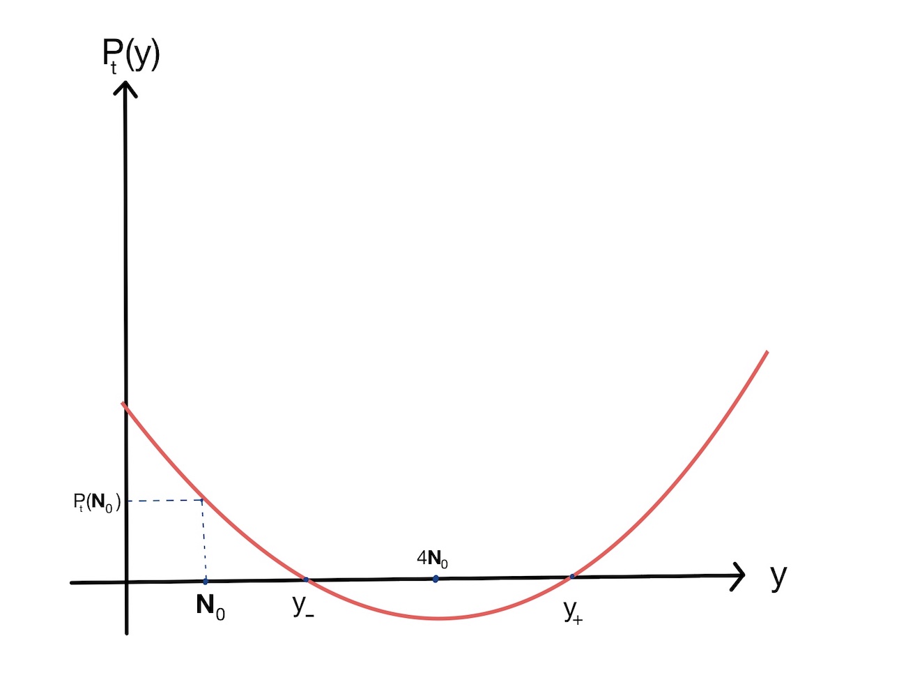
Figure 1. Positive real roots of the polynomial $P_{t}(y)$ for $t\ll 1$.

Taking $0<t\ll 1$ (for instance $0<t=\frac{1}{32C\mathsf{N}_{0}}$) we have (cf. Figure 1)

$$0<y_{-}=4\mathsf{N_{0}}\left(1-\sqrt{1/2}\right)<y_{+}=4\mathsf{N_{0}}\left(1+\sqrt{1/2}\right)$$

and

$$0<y_{-}<4\mathsf{N}_{0}<y_{+}.$$

Furthermore, the application $t\to\mathsf{E}_{t}$ is continuous for $t\in[0,T)$. This, together with the fact that $\mathsf{E}_{0}<\mathsf{N}_{0}$ and $\mathcal{P}_{t}(\mathsf{N}_{0})>0$, implies that

$$\forall t\in(0,t^{\star}),\quad\mathsf{E}_{T}<4\mathsf{N}_{0},$$ (70)

where $t^{\star}=\displaystyle\min\{\frac{1}{32C\mathsf{N}_{0}},1,T\}$.

Similarly as before, in order to perform the a priori estimates rigorously and construct the local existence of solutions we follow a regularization procedure. More precisely, the regularized version of (55) takes the form

$$w^{\epsilon}_{tt}+\mathscr{L}w^{\epsilon}=\left(\mathcal{J}^{\epsilon}\left((1+\mathcal{J}^{\epsilon}w^{\epsilon})\mathcal{J}^{\epsilon}w^{\epsilon}_{x}\right)+\left[\mathscr{L},\mathscr{N}w^{\epsilon}\right]w^{\epsilon}\right)_{x}-2\mathcal{J}^{\epsilon}\left((1+\mathcal{J}^{\epsilon}w^{\epsilon})\mathcal{J}^{\epsilon}w^{\epsilon}_{t}\right)_{x}.$$ (71)

Repeating the same a priori estimates for the regularized equation (71) we can deduce the analogue of (70) namely

$$\forall t\in(0,t^{\star}),\quad\mathsf{E}_{T}<4\mathsf{N}_{0},$$ (72)

where $t^{\star}=\displaystyle\min\{\frac{1}{32C\mathsf{N}_{0}},1,T^{\epsilon}\}$. Notice that the time of existence of the solution depends a priori on the regularization parameter $\epsilon$. Nevertheless, the following argument shows that (72) holds independently of the parameter $\epsilon$. Indeed, take $T^{\epsilon}$ the first time such that

$$\mathsf{E}_{T^{\epsilon}}=8\mathsf{N}_{0}.$$

We observe that the precise choice of the quantity $8\mathsf{N}_{0}$ is not special. One could choose also any other quantity bigger than $4\mathsf{N}_{0}$ to make the argument work. If the previous equality does not hold, that is, $\mathsf{E}_{T^{\epsilon}}<8\mathsf{N}_{0}$, this implies that $T^{\epsilon}=\infty,$ and hence we conclude (since $t^{\star}$ is the minimum) that $t^{\star}$ is independent of $\epsilon$. On the other hand if $T^{\epsilon}$ is finite then $t^{\star}=\displaystyle\min\{\frac{1}{32C\mathsf{N}_{0}},1,T^{\epsilon}\}=\displaystyle\min\{\frac{1}{32C\mathsf{N}_{0}},1\}$. Indeed, this assertion follows from invoking the continuity of $\mathsf{E}_{T}$ of the regularized problem, and using that by construction $\mathsf{E}_{T^{\epsilon}}=8\mathsf{N}_{0}$ and $\mathsf{E}_{t^{\star}}<4\mathsf{N}_{0}$. This concludes the proof. ∎

6. Well-posedness in Sobolev spaces for unidirectional non-local wave model

The main goal of this section is to prove the local well-posedness of equation (10) in $L^{2}$ based Sobolev spaces. Note first that, using (13), we have $-\mathscr{L}=\mathscr{Q}-1,$ and (10) can be rewritten as (we set $\varepsilon=1$ for simplicity)

$$h_{t}=-\frac{1}{2}\left(3hh_{x}+[\mathscr{Q},\mathscr{Q}h_{x}]h-\mathscr{Q}h_{x}-h_{x}\right).$$ (73)

For this equation, we show the following local well-posedness result.

Theorem 4.

Let $s>\frac{3}{2}$ and $h_{0}\in H^{s}(\mathbb{R})$ with mean zero. Then there exist $T_{\max}>0$ and a unique local solution $h\in C([0,T_{\max}),H^{s}(\mathbb{R}))$ of (73).

Proof.

The proof follows from the combination of appropriate a priori energy estimates and the use of a suitable approximation procedure using mollifiers, cf. [23]. Thus, we first focus in deriving a priori energy estimates and later comment briefly on the approximation procedure to construct the solution. We begin by reminding (cf. Section 3) that the mean property is conserved in time by the solutions

$$\int_{\mathbb{R}}h(x,t)\ dx=\int_{\mathbb{R}}h_{0}(x)\ dx,$$

as well as the $L^{2}$ norm

$$\int_{\mathbb{R}}h^{2}(x,t)\ dx=\int_{\mathbb{R}}h^{2}_{0}(x)\ dx.$$

Furthermore, applying $\Lambda^{s}$ to (73), multiplying by $\Lambda^{s}h$ and integrating we obtain

$$\frac{1}{2}\frac{d}{dt}\left\|h\right\|_{\dot{H}^{s}}^{2} =-\frac{3}{2}\int_{\mathbb{R}}\Lambda^{s}(hh_{x})\Lambda^{s}h\ dx-\frac{1}{2}\int_{\mathbb{R}}\Lambda^{s}\left([\mathscr{Q},\mathscr{Q}_{x}h]h\right)\Lambda^{s}h\ dx$$ (74)

$$\hskip 28.45274pt+\frac{1}{2}\int_{\mathbb{R}}\Lambda^{s}\mathscr{Q}h_{x}\Lambda^{s}h\ dx+\frac{1}{2}\int_{\mathbb{R}}\Lambda^{s}h_{x}\Lambda^{s}h\ dx.$$

Using the self-adjointness of the operator $\mathscr{Q}$, a straightforward computation shows that the last two terms on the right hand-side of (74) are zero. The first term can be estimated by means of the classical Kato-Ponce commutator as follows. Using integration by parts, we rewrite

$$\int_{\mathbb{R}}\Lambda^{s}(hh_{x})\Lambda^{s}h\ dx =\int_{\mathbb{R}}[\Lambda^{s},h]h_{x}\Lambda^{s}h\ dx+\int_{\mathbb{R}}h\Lambda^{s}h_{x}\Lambda^{s}h\ dx$$

$$=\int_{\mathbb{R}}[\Lambda^{s},h]h_{x}\Lambda^{s}h\ dx-\frac{1}{2}\int_{\mathbb{R}}h_{x}|\Lambda^{s}h|^{2}\ dx.$$

Now, invoking the first equation in Lemma 1.1 with $p=2,p_{1}=\infty,p_{2}=2$, we have that

$$\left|\int_{\mathbb{R}}\Lambda^{s}(hh_{x})\Lambda^{s}h\ dx\right| \lesssim\left\|[\Lambda^{s},h]h_{x}\right\|_{L^{2}}\left\|\Lambda^{s}h\right\|_{L^{2}}+\left\|h_{x}\right\|_{L^{\infty}}\left\|\Lambda^{s}h\right\|^{2}_{L^{2}}$$

$$\lesssim\left\|h_{x}\right\|_{L^{\infty}}\left\|\Lambda^{s}h\right\|^{2}_{L^{2}}.$$ (75)

The second term on the right hand side in (74) can be bounded as follows. Expanding the commutator and using the self-adjointness of $\mathscr{Q}$ yield

$$\int_{\mathbb{R}}\Lambda^{s}\left([\mathscr{Q},\mathscr{Q}_{x}h]h\right)\Lambda^{s}h\ dx =\int_{\mathbb{R}}\Lambda^{s}(\mathscr{Q}h_{x}h)\Lambda^{s}\mathscr{Q}h\ dx-\int_{\mathbb{R}}\Lambda^{s}(\mathscr{Q}h_{x}\mathscr{Q}h)\Lambda^{s}h\ dx.$$ (76)

Then applying the second estimate in Lemma 1.1 with $p=2,p_{1},p_{3}=\infty,p_{2},p_{4}=2$, the Sobolev embedding $H^{\frac{1}{2}+\epsilon}(\mathbb{R})\hookrightarrow L^{\infty}(\mathbb{R})$ for $\epsilon>0$, and the fact that $\mathscr{Q}$ is continuous between $H^{s}(\mathbb{R})$ and $H^{s+2}(\mathbb{R})$ for any $s\in\mathbb{R}$ we find that

$$\left|\int_{\mathbb{R}}\Lambda^{s}(\mathscr{Q}h_{x}h)\Lambda^{s}\mathscr{Q}h\ dx\right| \lesssim\left\|\Lambda^{s}(\mathscr{Q}h_{x}h)\right\|_{L^{2}}\left\|\Lambda^{s}\mathscr{Q}h\right\|_{L^{2}}$$

$$\lesssim\left(\left\|\Lambda^{s}\mathscr{Q}h_{x}\right\|_{L^{\infty}}\left\|h\right\|_{L^{2}}+\left\|\mathscr{Q}h_{x}\right\|_{L^{\infty}}\left\|\Lambda^{s}h\right\|_{L^{2}}\right)\left\|\Lambda^{s}\mathscr{Q}h\right\|_{L^{2}}$$

$$\lesssim\left(\left\|h\right\|_{H^{s-\frac{1}{2}+\epsilon}}\left\|h\right\|_{L^{2}}+\left\|h\right\|_{H^{-\frac{1}{2}+\epsilon}}\left\|h\right\|_{H^{s}}\right)\left\|h\right\|_{H^{s-2}}.$$

Similarly, one can show that

$$\left|\int_{\mathbb{R}}\Lambda^{s}(\mathscr{Q}h_{x}\mathscr{Q}h)\Lambda^{s}h\ dx\right|\lesssim\left(\left\|h\right\|_{H^{s-\frac{1}{2}+\epsilon}}\left\|h\right\|_{H^{-2}}+\left\|h\right\|_{H^{-\frac{1}{2}+\epsilon}}\left\|h\right\|_{H^{s-2}}\right)\left\|h\right\|_{H^{s}}.$$

Thus,

$$\left|\int_{\mathbb{R}}\Lambda^{s}\left([\mathscr{Q},\mathscr{Q}_{x}h]h\right)\Lambda^{s}h\ dx\right|\leq C\left\|h_{0}\right\|_{L^{2}}\left(\left\|h\right\|_{H^{s-\frac{1}{2}+\epsilon}}+\left\|h\right\|_{H^{s-2}}\right)\left\|h\right\|_{H^{s}}$$ (77)

where we have used that $\left\|h\right\|_{H^{-\frac{1}{2}+\epsilon}}+\left\|h\right\|_{H^{-2}}\leq C\left\|h\right\|_{L^{2}}=C\left\|h_{0}\right\|_{L^{2}}$, for some constant $C$.

Therefore, combining estimates (75), (77) leads to

$$\frac{d}{dt}\left\|h\right\|_{H^{s}}^{2}\leq C\left\|h_{x}\right\|_{L^{\infty}}\left\|h\right\|_{H^{s}}^{2}+C\left\|h_{0}\right\|_{L^{2}}\left(\left\|h\right\|_{H^{s-\frac{1}{2}+\epsilon}}+\left\|h\right\|_{H^{s-2}}\right)\left\|h\right\|_{H^{s}}$$ (78)

which in particular gives the following inequality

$$\frac{d}{dt}\left\|h\right\|_{H^{s}}^{2}\leq C\left(\left\|h_{x}\right\|_{L^{\infty}}+1\right)\left\|h\right\|_{H^{s}}^{2}.$$ (79)

Using the Sobolev embedding $H^{\frac{1}{2}+\epsilon}(\mathbb{R})\hookrightarrow L^{\infty}(\mathbb{R})$, $\epsilon>0$, we observe that

$$\frac{d}{dt}\left\|h\right\|_{H^{s}}^{2}\leq C\left\|h\right\|_{H^{s}}^{3},$$ (80)

for some constant $C$ independent of $t$. Defining $\mathcal{E}(t)=\left\|h\right\|_{H^{s}}^{2}$, estimate (80) leads to the following differential equation

$$\mathcal{E}^{\prime}(t)\leq C\mathcal{E}^{3/2}(t),$$ (81)

with $C=C_{s}>0$ which ensures a uniform time of existence $T_{\max}>0$ such that

$$\mathcal{E}(t)\leq 4\mathcal{E}(0),0<t<T_{\max}.$$

Once this uniform time of existence has been obtained, the local existence result follows classical regularization procedure (cf. [23]) as follows. First, we consider a symmetric and positive mollifier $\mathcal{J}\in C^{\infty}_{c}$, $\mathcal{J}(x)=J(|x|)$ such that $\int_{\mathbb{R}}\mathcal{J}=1$. For $\epsilon>0$ we define $\mathcal{J}^{\epsilon}=\frac{1}{\epsilon}\mathcal{J}(\frac{x}{\epsilon})$ and consider the regularized problem

$$\partial_{t}h^{\epsilon}=-\frac{1}{2}\big{(}\mathcal{J}^{\epsilon}(\mathcal{J}^{\epsilon}h\partial_{x}\mathcal{J}^{\epsilon}h)+[\mathscr{Q},\mathscr{Q}h^{\epsilon}_{x}]h^{\epsilon}-\mathscr{Q}h^{\epsilon}_{x}-\mathcal{J}^{\epsilon}\mathcal{J}^{\epsilon}h^{\epsilon}_{x}\big{)}.$$ (82)

In (82), the conserved quantities are also preserved by the flow and the previous bounds (75)-(77) and thus (78) hold. Therefore, we may find a time of existence $T^{\star}>0$ for the sequence of regularized problems. Using compactness arguments and passing to the limit conclude the proof of existence. The continuity in time for the solution (instead of merely weak continuity) is obtained by classical arguments (cf. [23]): On the one hand, the differential equation (81) yields the strong right continuity at $t=0$. On the other hand, it is easy to check that changing variables $\tilde{t}=-t$, we can repeat once again the same bounds and provide the strong left continuity at $t=0$. Combining both arguments shows the continuity in time of the solution.

As for uniqueness, let $h^{1},h^{2}\in C([0,T_{\max}),H^{s}(\mathbb{R}))$ be two solutions corresponding to the same initial condition and denote $\widehat{h}=h^{2}-h^{1}$. Then $\widehat{h}$ satisfies

$$\partial_{t}\widehat{h}=-\frac{1}{2}\left(3h^{2}h^{2}_{x}-3h^{1}h^{1}_{x}+[\mathscr{Q},\mathscr{Q}h^{2}_{x}]h^{2}-[\mathscr{Q},\mathscr{Q}h^{1}_{x}]h^{1}-\mathscr{Q}\widehat{h}_{x}-\widehat{h}_{x}\right).$$ (83)

Then, multiplying (83) by $\widehat{h}$ and integrating, we have

$$\frac{1}{2}\frac{d}{dt}\left\|\widehat{h}\right\|_{L^{2}}^{2}=-\frac{3}{2}\int_{\mathbb{R}}\left(\widehat{h}h^{2}_{x}+h^{1}\widehat{h}_{x}\right)\widehat{h}\ dx+\int_{\mathbb{R}}\bigg{[}[\mathscr{Q},\mathscr{Q}h^{2}_{x}]h^{2}-[\mathscr{Q},\mathscr{Q}h^{1}_{x}]h^{1}\bigg{]}\widehat{h}\ dx.$$

Using (27b), it is not hard to check that each commutator can be rewritten as a Burgers-type nonlinear-term and therefore

$$\left|\int_{\mathbb{R}}\bigg{[}[\mathscr{Q},\mathscr{Q}h^{2}_{x}]h^{2}-[\mathscr{Q},\mathscr{Q}h^{1}_{x}]h^{1}\bigg{]}\widehat{h}\ dx\right| \leq C\left(\left\|h^{1}\right\|_{L^{\infty}}+\left\|h^{2}\right\|_{L^{\infty}}\right)\left\|\widehat{h}\right\|_{L^{2}}^{2}\leq C,$$

for some constant $C$. Similarly, integrating by parts,

$$\left|\int_{\mathbb{R}}\left(\widehat{h}h^{2}_{x}+h^{1}\widehat{h}_{x}\right)\widehat{h}\ dx\right|\leq C\left(\left\|\partial_{x}h^{1}\right\|_{L^{\infty}}+\left\|\partial_{x}h^{2}\right\|_{L^{\infty}}\right)\left\|\widehat{h}\right\|_{L^{2}}^{2}.$$

Defining $\beta(t)=\left\|h^{1}\right\|_{L^{\infty}}+\left\|h^{2}\right\|_{L^{\infty}}+\left\|\partial_{x}h^{1}\right\|_{L^{\infty}}+\left\|\partial_{x}h^{2}\right\|_{L^{\infty}}$, then

$$\frac{1}{2}\frac{d}{dt}\left\|\widehat{h}\right\|_{L^{2}}^{2}\leq C\beta(t)\left\|\widehat{h}\right\|_{L^{2}}^{2}.$$

Uniqueness holds applying Grönwall inequality. ∎

Remark 1.

One can readily check that a direct consequence of the derived estimates in the proof of Theorem 4 provides the following blow-up criterion when combined with the logarithmic Sobolev inequality (cf. Lemma 1.2) which we state as a theorem for the sake of clarity.

Theorem 5 (Blow-up criteria).

Let $s>\frac{3}{2}$, $h_{0}\in H^{s}(\mathbb{R})$ with zero mean and let $T_{\max}>0$ be the lifespan associated to the solution $h$ to (73) with $h(x,0)=h_{0}(x)$. Then $h$ blows-up in finite time $T_{\max}$ if and only if

$$\int_{0}^{T_{\max}}\left\|h_{x}(\tau)\right\|_{\text{BMO}}\ d\tau=\infty.$$ (84)

Proof.

The result follows as a direct consequence of estimate (79). Using the logarithmic inequality in Lemma 1.2 we find that

$$\frac{d}{dt}\left\|h\right\|_{H^{s}}\leq C\left(1+\left\|h_{x}\right\|_{\text{BMO}}\big{[}1+\displaystyle\log(1+\left\|h\right\|_{H^{s}})\big{]}\right)\left\|h\right\|_{H^{s}},$$ (85)

for some constant $C$. From (85), it holds that

$$1+\left\|h\right\|_{H^{s}}\leq\bigg{[}(1+\left\|h_{0}\right\|_{H^{s}})\mbox{exp}\left(1+CT_{\max}\right)\bigg{]}^{\mbox{exp}\left(C\int_{0}^{T_{\max}}(\left\|h_{x}(\tau)\right\|_{\text{BMO}}\ d\tau\right)}.$$

Therefore, if there exists $L>0$ such that

$$\int_{0}^{T_{\max}}\left\|h_{x}(\tau)\right\|_{\text{BMO}}\ d\tau<L,$$

then

$$1+\left\|h\right\|_{H^{s}}\leq\bigg{[}(1+\left\|h_{0}\right\|_{H^{s}})\mbox{exp}\left(1+CT_{\max}\right)\bigg{]}^{\mbox{exp}\left(CL\right)}.$$

On the contrary, if $\int_{0}^{T_{\max}}\left\|h_{x}(t)\right\|_{\text{BMO}}\ dt=\infty$, by means of the embedding $H^{\frac{1}{2}}(\mathbb{R})\subset\text{BMO}(\mathbb{R})$, we deduce that the solution $h(x,t)$ will blow up in finite time and (84) follows. ∎

7. A wave breaking result for the unidirectional non-local wave model

In this section, we investigate the possible wave breaking phenomena for equation (10), that is, the formation of an infinite slope in the solution in the $x$-direction. As we did for the well-posedness result in Section 6, it is more convenient to work with the alternative formulation (73). The following lemma shows that for the maximal time of existence $T_{\max}>0$, we have that the solutions remains bounded. More precisely,

Lemma 7.1.

Let $s>{7/2}$, $h_{0}\in H^{s}(\mathbb{R})$, and let $T_{max}>0$ be the maximal time of existence of the unique solution $h$ of (73) given by Theorem 4. Then

$$\sup_{t\in[0,T_{\max})}\left\|h(t)\right\|_{L^{\infty}(\mathbb{R})}<\infty.$$ (86)

Proof.

To establish the $L^{\infty}$ bound, we follow a pointwise method (cf. [6, 7]). Due to Theorem 4, we have that $h\in C([0,T_{\max}),H^{s})\cap C^{1}([0,T_{\max}),H^{s-1})$, hence by the Sobolev embedding theorem, if $s>7/2$ we have that $h\in C^{1}([0,T_{\max})\times\mathbb{R})$. In particular,

$$m(t)=\displaystyle\inf_{x\in\mathbb{R}}h(x,t)=h(\underline{x}_{t},t),\quad M(t)=\displaystyle\sup_{x\in\mathbb{R}}h(x,t)=h(\overline{x}_{t},t),\mbox{ for }t>0,$$

(for some $\underline{x}_{t},\overline{x}_{t}$) are Lipschitz functions. Following [7], one can readily check that $M(t)$ satisfies

$$\left|M(t)-M(s)\right| =\left\{\begin{array}[]{cc}h(\overline{x}_{t},t)-h(\overline{x}_{s},s)\text{ if }M(t)>M(s)\\ h(\overline{x}_{s},s)-h(\overline{x}_{t},t)\text{ if }M(s)>M(t)\end{array}\right.$$

$$\leq\left\{\begin{array}[]{cc}h(\overline{x}_{t},t)-h(\overline{x}_{t},s)\text{ if }M(t)>M(s)\\ h(\overline{x}_{s},s)-h(\overline{x}_{s},t)\text{ if }M(s)>M(t)\end{array}\right.$$

$$\leq\left\{\begin{array}[]{cc}|\partial_{t}h(\overline{x}_{t},z)||t-s|\text{ if }M(t)>M(s)\\ |\partial_{t}h(\overline{x}_{s},z)||t-s|\text{ if }M(s)>M(t)\end{array}\right.$$

$$\leq\max_{y,z}|\partial_{t}h(y,z)||t-s|.$$

Similarly

$$\left|m(t)-m(s)\right|\leq\max_{y,z}|\partial_{t}h(y,z)||t-s|.$$

From Rademacher’s theorem it holds that $M(t)$ and $m(t)$ are differentiable in $t$ almost everywhere. Furthermore

$$M^{\prime}(t) =\lim_{\delta\rightarrow 0}\frac{h(\overline{x}_{t+\delta},t+\delta)-h(\overline{x}_{t},t)}{\delta}=\lim_{\delta\rightarrow 0}\frac{h(\overline{x}_{t+\delta},t+\delta)-h(\overline{x}_{t},t)\pm h(\overline{x}_{t+\delta},t)}{\delta}$$

$$\leq\lim_{\delta\rightarrow 0}\frac{h(\overline{x}_{t+\delta},t+\delta)-h(\overline{x}_{t+\delta},t)}{\delta}\leq\partial_{t}h(\overline{x}_{t},t).$$

In a similar fashion, we obtain that

$$M^{\prime}(t) =\lim_{\delta\rightarrow 0}\frac{h(\overline{x}_{t+\delta},t+\delta)-h(\overline{x}_{t},t)}{\delta}=\lim_{\delta\rightarrow 0}\frac{h(\overline{x}_{t+\delta},t+\delta)-h(\overline{x}_{t},t)\pm h(\overline{x}_{t},t+\delta)}{\delta}$$

$$\geq\lim_{\delta\rightarrow 0}\frac{h(\overline{x}_{t},t+\delta)-h(\overline{x}_{t},t)}{\delta}\geq\partial_{t}h(\overline{x}_{t},t).$$

As a consequence

$$M^{\prime}(t)=\partial_{t}h(\overline{x}_{t},t)\text{ a.e.}$$ (87)

Similarly

$$m^{\prime}(t)=\partial_{t}h(\underline{x}_{t},t)\text{ a.e.}$$

Therefore, from (87), evaluating (73) at $x=\overline{x}_{t}$ and noticing that $h_{x}(\overline{x}_{t},t)=0$, we have

$$M^{\prime}(t)=-\frac{1}{2}\left([\mathscr{Q},\mathscr{Q}h_{x}(\overline{x}_{t})]h(\overline{x}_{t})-\mathscr{Q}h_{x}(\overline{x}_{t})\right).$$ (88)

Moreover, from (12), the estimates

$$\left\|G\right\|_{L^{\infty}}=\frac{1}{2},\quad\left\|\partial_{x}G\right\|_{L^{\infty}}=\frac{1}{2},$$

and Young’s inequality, it holds that

$$\mathscr{Q}h(x_{t}) \leq\left\|G\right\|_{L^{\infty}(\mathbb{R})}\left\|h\right\|_{L^{2}(\mathbb{R})}=\frac{1}{2}\left\|h\right\|_{L^{2}(\mathbb{R})},$$ (89)

$$[\mathscr{Q},\mathscr{Q}h_{x}(x_{t})]h(x_{t}) \leq\left\|G\right\|_{L^{\infty}(\mathbb{R})}\left\|\mathscr{Q}h_{x}h\right\|_{L^{2}(\mathbb{R})}+\left\|\mathscr{Q}h_{x}\right\|_{L^{\infty}(\mathbb{R})}\left\|\mathscr{Q}h\right\|_{L^{\infty}(\mathbb{R})}\leq\frac{1}{2}\left\|h\right\|_{L^{2}}^{2}.$$ (90)

From (88), the estimates (89), (90) and the preservation of the $L^{2}$ norm by the solutions of (73) imply that

$$M^{\prime}(t)\leq\frac{1}{4}\left(1+\left\|h_{0}\right\|_{L^{2}}^{2}\right),$$

and therefore

$$M(t)\leq M(0)+\frac{1}{4}\left(1+\left\|h_{0}\right\|_{L^{2}}^{2}\right)t.$$ (91)

for $t\in[0,T_{\max})$. In a similar way, we have

$$m(t)\geq m(0)-\frac{1}{4}\left(1+\left\|h_{0}\right\|_{L^{2}}^{2}\right)t.$$ (92)

for $t\in[0,T_{\max})$. Thus combining (91) and (92) we conclude that

$$\sup_{t\in[0,T_{\max})}\left\|h(t)\right\|_{L^{\infty}(\mathbb{R})}\leq\left\|h_{0}\right\|_{L^{\infty}(\mathbb{R})}+\frac{1}{4}\left(1+\left\|h_{0}\right\|_{L^{2}}^{2}\right)T_{\max}<\infty,$$ (93)

and (86) holds. ∎

Next, let us state the wave breaking result.

Theorem 6.

Let $s>{\frac{9}{2}},h_{0}\in H^{s}(\mathbb{R})$, and let $h$ be the solution of the ivp of (73) with initial condition $h_{0}$. Assume that

$$\inf_{x\in\mathbb{R}}h_{0,x}(x)\leq-H_{0},$$ (94)

for some positive constant $H_{0}$, which depends on $\left\|h_{0}\right\|_{L^{2}(\mathbb{R})},\|h_{0}\|_{L^{\infty}}$ and specified below. Then there exists $T_{b}<\infty$ such that

$$\lim\inf_{t\to T_{b}}\left(\inf_{x\in\mathbb{R}}h_{x}(x,t)\right)=-\infty.$$ (95)

Proof.

Similarly as in the proof of Lemma 7.1, we follow a pointwise method to derive an ODE which breaks down in finite time. Again, due to Theorem 4, we have that $h\in C([0,T_{\max}),H^{s})\cap C^{1}([0,T_{\max}),H^{s-1})$, hence by the Sobolev embedding theorem, if $s>9/2$ then $h_{x}\in C^{1}([0,T_{\max})\times\mathbb{R})$. We begin by setting

$$m(t)=\displaystyle\inf_{x\in\mathbb{R}}h_{x}(x,t)=h_{x}(\underline{x}_{t},t),\quad\mbox{for }t\in[0,T_{\max}),$$

for some $\underline{x}_{t}$. Arguing as in Lemma 7.1, one can check that $m(t)$ is Lipschitz and hence via Radamacher’s Theorem it is inferred that

$$m^{\prime}(t)=\partial_{t}h_{x}(\underline{x}_{t},t),\ \mbox{a.e}.$$

Differentiating (73) with respect to $x$ and using (46) yield

$$h_{xt}=-\frac{1}{2}\left(3h_{x}^{2}+3hh_{xx}+\partial_{x}[\mathscr{Q},\mathscr{Q}h_{x}]h-\mathscr{Q}h+h-h_{xx}\right).$$ (96)

Evaluating (96) at $x=\underline{x}_{t}$ and noticing that $h_{xx}(\underline{x}_{t},t)=0$ we have

$$m^{\prime}(t)=-\frac{3}{2}m(t)^{2}+\mathcal{K}(t),$$ (97)

with

$$\mathcal{K}(t)=\frac{1}{2}\big{(}\partial_{x}[\mathscr{Q},\mathscr{Q}h_{x}]h(\underline{x}_{t},t)-\mathscr{Q}h(\underline{x}_{t},t)+h(\underline{x}_{t},t)\big{)}.$$

We now estimate the quantity $\mathcal{K}(t)$. First notice, from (12), that

$$\left\|\mathscr{Q}h+h\right\|_{L^{\infty}}\leq\left\|G\star h\right\|_{L^{\infty}}+\left\|h\right\|_{L^{\infty}}\leq\left\|G\right\|_{L^{\infty}}\left\|h\right\|_{L^{2}}=\frac{1}{2}\left\|h\right\|_{L^{2}}+\left\|h\right\|_{L^{\infty}}.$$ (98)

On the other hand, from the Sobolev embedding $H^{\frac{1}{2}+\epsilon}(\mathbb{R})\hookrightarrow L^{\infty}(\mathbb{R})$ for $\epsilon>0$ and the fact that $\mathscr{Q}$ is continuous between $H^{s}(\mathbb{R})$ and $H^{s+2}(\mathbb{R})$ for any $s\in\mathbb{R}$, then the commutator term is bounded by

$$\partial_{x}[\mathscr{Q},\mathscr{Q}h_{x}]h(\underline{x}_{t},t)\leq\left\|[\mathscr{Q},\mathscr{Q}h_{x}]h\right\|_{H^{\frac{1}{2}+\epsilon}(\mathbb{R})}\leq\left\|\mathscr{Q}h_{x}h\right\|_{H^{-\frac{3}{2}+\epsilon}(\mathbb{R})}+\left\|(\mathscr{Q}h)^{2}\right\|_{H^{\frac{3}{2}+\epsilon}}.$$ (99)

The first term on the right hand-side of (99) is bounded by

$$\left\|\mathscr{Q}h_{x}h\right\|_{H^{-\frac{3}{2}+\epsilon}}\leq C\left\|h\right\|_{L^{2}(\mathbb{R})}^{2},$$ (100)

and the second term can be estimated from the Sobolev algebra property as

$$\left\|(\mathscr{Q}h)^{2}\right\|_{H^{\frac{3}{2}+\epsilon}}\leq C\left\|\mathscr{Q}h\right\|^{2}_{H^{\frac{3}{2}+\epsilon}}\leq C\left\|h\right\|^{2}_{L^{2}(\mathbb{R})},$$ (101)

for some constant $C$. The bounds (98)-(101), the $L^{\infty}$ estimate (93), and the time preservation of the $L^{2}$ norm by $h$ lead to

$$\mathcal{K}(t) \leq C\left(\left\|h\right\|^{2}_{L^{2}(\mathbb{R})}+\left\|h\right\|_{L^{2}(\mathbb{R})}+\left\|h\right\|_{L^{\infty}(\mathbb{R})}\right)$$

$$\leq C\big{(}\left\|h_{0}\right\|_{L^{\infty}(\mathbb{R})}+\left(1+\left\|h_{0}\right\|_{L^{2}}^{2}\right)(t+1)\big{)}.$$ (102)

Using (102), then (97) implies

$$m^{\prime}(t)\leq-\frac{3}{2}m(t)^{2}+A+Bt,$$ (103)

where $A$ and $B$ are the positive constants, depending on $\left\|h_{0}\right\|_{L^{\infty}},\left\|h_{0}\right\|_{L^{2}}$, determined in (102).

In order to show the wave breaking result, let us assume that the initial data is such that (cf. [28])

$$m(0)\leq-C,$$ (104)

for some positive constant $C$ such that $C^{2}>4A$. Then $2A-m(0)^{2}/2<0$ and

$$m^{\prime}(t)\bigg{|}_{t=0}\leq-m(0)^{2}-\frac{1}{2}m(0)^{2}+2A\leq-m(0)^{2}<0.$$

Therefore there exists a sufficiently small $0<\delta$ such that $m^{\prime}(t)<0$, for $0\leq t<\delta$. This implies $m(t)<m(0)\leq-C$ and similarly $2A-m(t)^{2}/2<0$ for $0\leq t<\delta$. Thus, if $0<t\leq\min\{\delta,A/B\}$ from (103) it holds that

$$m^{\prime}(t)\leq-m(t)^{2}-\frac{1}{2}m(t)^{2}+2A\leq-m(t)^{2}.$$

This leads to

$$m(t)\leq\frac{m(0)}{m(0)t+1}.$$ (105)

Taking the initial datum such that

$$\frac{1}{-m(0)}\leq\frac{A}{B},$$ (106)

note that (104), (106) define a constant $H_{0}$ for which $m(0)$ satisfies (94), and (105) implies the existence of a time $T_{b}$ where (95) holds. ∎

References

- [1] D. Alonso-Orán. Asymptotic shallow models arising in magnetohydrodynamics, Water Waves, 3, 371–398 (2021).
- [2] Y. A. Berezin, V. Karpman. Theory of nonstationary finite-amplitude waves in a low-density plasma, Sov. Phys. JETP 19 1265–1271 (1964).
- [3] A. Castro, D. Lannes. Fully nonlinear long-wave models in the presence of vorticity, J. Fluid Mech. 759 (2014) 642–675 (2014).
- [4] A. Castro, D. Lannes. Well-posedness and shallow-water stability for a new Hamiltonian formulation of the water waves equations with vorticity, Indiana Univ. Math. J., 64 (4), 1169–1270 (2015).
- [5] A. Cheng, R. Granero-Belinchón, S. Shkoller, J. Wilkening. Rigorous Asymptotic Models of Water Waves, Water Waves, 1, 71–130, (2019).
- [6] A. Constantin, J. Escher. Wave breaking for nonlinear nonlocal shallow water equations, Acta Math., 181, 229 243, (1998).
- [7] A. Córdoba, D. Córdoba . A maximum principle applied to quasi-geostrophic equations, Communications in Mathematical Physics, 249(3):511–528, (2004).
- [8] D. Coutand, S. Shkoller. The Interaction between Quasilinear Elastodynamics and the Navier-Stokes Equations , Arch. Rational Mech. Anal., 179, 303–352 (2006).
- [9] W. Craig, D. Lannes, C. Sulem. Water waves over a rough bottom in the shallow water regime, Ann. Inst. H. Poincaré Anal. Non Linéaire, 29 (2) 233–259 (2012).
- [10] H. Dong. Well-posedness for a transport equation with nonlocal velocity. Journal of Functional Analysis, 255(11):3070–3097, (2008).
- [11] G. Fornberg, G.B. Whitham. A numerical and theoretical study of certain nonlinear wave phenomena, Philos. Trans. Roy. Soc. London Ser. A, 289 no. 1361, 373–404, (1978).
- [12] C. Gardner, G. Morikawa. Similarity in the asymptotic behavior of collision-free hydromagnetic waves and water waves, Tech. rep., New York Univ., New York. Inst. of Mathematical Sciences (1960).
- [13] R. Granero-Belinchón, S. Scrobogna. Asymptotic models for free boundary flow in porous media, Physica D: Nonlinear Phenomena, 392, 1-16,(2019).
- [14] R. Granero-Belinchón, S. Shkoller. A model for Rayleigh-Taylor mixing and interface turn-over, Multiscale Modeling and Simulation, 15 (1), 274–308 (2017).
- [15] S. V. Haziot. Wave breaking for the Fornberg–Whitham equation, J. Differential Equations, 263 no.12, (2017).
- [16] J. Holmes. Well-Posedness of the Fornberg-Whitham equation on the circle, J. Differential Equations,260 no.12, 8530–8549, (2016).
- [17] J. Holmes and R. C. Thompson Well-posedness and continuity properties of the Fornberg–Whitham equation in Besov spaces. J. Differential Equations, 263 no.7, (2017).
- [18] G. Hörmann. Solution concepts, well-posedness, and wave breaking for the Fornberg–Whitham equation, Monatsh Math , 195, 421–449, (2021).
- [19] K. Itasaka. Wave-breaking phenomena and global existence for the generalized Fornberg–Whitham equation, Journal of Mathematical Analysis and Applications, 502, Issue 1, (2021).
- [20] T. Kakutani, H. Ono, T. Taniuti, C.-C. Wei. Reductive perturbation method in nonlinear wave propagation ii. application to hydromagnetic waves in cold plasma, Journal of the Physical Society of Japan, 24 (5) 1159–1166 (1968).
- [21] T. Kato and G. Ponce. Commutator estimates and the Euler and Navier-Stokes equations. Communications on Pure and Applied Mathematics, 41(7):891–907, (1988).
- [22] C. E. Kenig, G. Ponce, and L. Vega. Well-posedness of the initial value problem for the Korteweg-de Vries equation, Journal of the American Mathematical Society, 4(2):323–347, (1991).
- [23] A. J. Majda, L. Bertozzi. Vorticity and Incompressible Flow, Cambridge Texts in Applied Mathematics , Cambridge University Press, Cambridge, (2001).
- [24] X. Pu, M. Li. Kdv limit of the hydromagnetic waves in cold plasma, Zeitschrift für angewandte Mathematik und Physik, 70 (1), 32, (2019).
- [25] C. H. Su, C. S. Gardner. Korteweg-de vries equation and generalizations. iii. derivation of the korteweg-de vries equation and burgers equation, Journal of Mathematical Physics, 10 (3), 536–539 (1969).
- [26] E. M. Stein. Singular Integrals and Differentiability Properties of Functions, Princeton University Press, (1970).
- [27] E. M. Stein. Harmonic Analysis: Real Variable Methods, Orthogonality and Oscillatory Integrals, Princeton Math. Series 43, Princeton Univ. Press, Princeton, NJ, (1993).
- [28] L. Wei. New wave-breaking criteria for the Fornberg-Whitham equation, J.of Differential Equations, 280, 571–589, (2021).
- [29] G. B. Whitham. Linear and Nonlinear Waves, John Wiley & Sons, New York, (1974).
- [30] S. Yang. Wave Breaking Phenomena for the Fornberg–Whitham Equation, J. Dyn. Diff. Equat., 33, 1753–1758, (2021).