Do Physics-informed Neural Networks Satisfy Local and Global Mass Balance?

Abstract: Physics-informed neural networks (PINN) have recently become attractive to solve partial differential equations (PDEs) that describe physics laws. By including PDE-based loss functions, physics laws such as mass balance are enforced softly. In this paper, we examine how well mass balance constraints are satisfied when PINNs are used to solve the resulting PDEs. We investigate PINN’s ability to solve the 1D saturated groundwater flow equations for homogeneous and heterogeneous media and evaluate the local and global mass balance errors. We compare the obtained PINN’s numerical solution and associated mass balance errors against a two-point finite volume numerical method and the corresponding analytical solution. We also evaluate the accuracy of PINN to solve the 1D saturated groundwater flow equation with and without incorporating hydraulic head as training data. Our results showed that one needs to provide hydraulic head data to obtain an accurate solution for the head for the heterogeneous case. That is, only after adding data at some collocation points the PINN methodology was able to give a solution close to the finite volume and analytical solutions. In addition, we demonstrate that even after adding hydraulic head data at some collocation points, the resulting local mass balance errors are still significant at the other collocation points compared to the finite volume approach. Tuning the PINN’s hyperparameters such as the number of collocation points, epochs, and learning rate did not improve the solution accuracy or the mass balance errors compared to the finite volume solution. Mass balance errors may pose a significant challenge to PINN’s utility for applications where satisfying physical and mathematical properties is crucial.

Keywords: PINN, physics-informed neural networks, mass balance errors, porous media flow, analytical and numerical modeling.

1   Introduction

Partial differential equations (PDEs) represent physical laws describing natural and engineered systems, e.g., heat transfer, fluid flow, wave propagation, etc., and are widely used to predict physical variables of interest in natural and engineered phenomena in both spatial and temporal domains. Often, the PDE solutions are combined with laboratory and field experiments to help stakeholders make informed decisions. Therefore, accurate estimation of variables of interest is critical. Numerous methods are used to solve PDEs, including analytical [1, 2, 3], finite difference [4, 5], finite volume [6, 7, 5], finite element [5, 8].

Recently, due to the advances in machine learning (ML) and physics-informed machine learning methods (PIML), physics-informed neural networks (PINN) [9, 10, 11, 12, 13] are gaining popularity as a tool to solve PDEs. In this approach, one treats the primary variable in the PDE to be solved as a neural network. Then, using auto-differentiation, the underlying PDE of interest is discretized, and modern optimization frameworks are used to minimize a loss function. It captures losses due to the PDE residual along with the losses due to the initial and boundary conditions. PINN has been used to solve numerous scientific and engineering problems [11, 9, 10, 14, 12, 13, 15, 16, 17, 18, 19, 20, 21, 22, 23]. These examples in literature have demonstrated that PINN can handle complex geometry well. However, it has been shown that PINN’s training is computationally expensive, and the resulting solution is not always accurate compared to its counterpart numerical solutions [21, 24, 25, 26]. For instance, the training process can take 10000s of epochs, and the absolute error of forward solutions is $\approx 10^{-5}$ because of the challenges involved in solving high-dimensional non-convex optimization problems [25, 27].

Several studies have addressed PINN’s drawbacks in the areas of computational time and accuracy. For instance, Jagtap et al., [24] address the accuracy of PINN by imposing continuity/flux across the boundary of subdomains as a constraint through an additional term to the loss function. However, the additional term in the loss function makes the model more complicated to train and requires more data with increased computational cost. Huang et al., [28] looked at improving the training efficiency by incorporating multi-resolution hash encoding into PINN that offers locally-aware coordinate inputs to the neural network. This encoding method requires careful selection of hyperparameters and auto-differentiation, complicating the training and post-training processes.

However, there is no systematic study on how PINN solutions perform with regard to satisfying the balance laws such as mass, momentum, or energy. In this study, we interrogate the performance of PINN solutions in terms of satisfying the balance of mass. We chose the application of groundwater flow where the mass flux is linearly related to the gradients in the head through Darcy’s model. We used PINN to solve simple boundary value PDEs describing 1D steady-state saturated groundwater flow in both homogeneous and heterogeneous confined aquifers. For comparison, we solved the same governing equations analytically and via a traditional numerical method called two-point finite volume (FV) method [7].

The outline of our paper is as follows: Sec. 2 provides the governing equations for groundwater flow and equations for mass balance error calculation. Section 3 presents the analytical, two-point flux finite volume, and PINN solutions for the governing equations described in Sec. 2. Section 4 discusses PINN training; compares the analytical, finite volume, and PINN solutions for the hydraulic head; Darcy’s flux; and mass balance error. Finally, conclusions are drawn in Sec. 5.

2   Governing Equations

The one-dimensional steady-state balance of mass for groundwater flow in the absence of sources and sinks within the flow domain is:

$$\frac{\partial}{\partial{x}}\left[{{q}(x)}\right]=0,$$ (1)

where, $q(x)$, follows the Darcy’s model given by :

$${q}(x)=-K(x)\frac{{\partial{h}}}{{\partial{x}}},$$ (2)

where, $h[L]$ is the piezometric head, $x[L]$ is the coordinate, and $K[L/T]$ is the hydraulic conductivity. Using Eqs. 1 and 2, the balance of mass governing equation reduces to:

$$\frac{\partial}{{\partial{x}}}\left[{K\left(x\right)\frac{\partial}{{\partial x}}h(x)}\right]=0.$$ (3)

Eq. 3 requires two boundary conditions for head. Assuming a unit length domain, if $h_{L},h_{R}$ are the heads at the left and the right faces of the domain, then $h(x=0)=h_{L}$ and $h(x=1)=h_{R}$.

The model domain ($x\in[0,1]$) is discretized into a finite number of cells ($NCells$). Figure 1 shows the discretization for obtaining both the FV and PINN solutions. Assuming a unit area for the one-dimensional domain, the mass flux at face $i-\frac{1}{2}$ ($m_{\mathrm{local}_{i-\frac{1}{2}}}$), the local mass balance error (LMBE) in cell $i$, and the global mass balance error (GMBE) are:

$$m_{\mathrm{local}_{i-\frac{1}{2}}} =\rho_{w}q_{i-\frac{1}{2}},$$ (4a)

$$LMBE_{i} ={m_{\mathrm{local}}}_{i+\frac{1}{2}}-{m_{\mathrm{local}}}_{i-\frac{1}{2}}\quad\forall i=1,2,\cdots,NCells,$$ (4b)

$$GMBE =\sum\limits_{i=1}^{NCells}LMBE_{i},$$ (4c)

where, ${\rho_{w}}$ $[M/L^{3}]$ is the density of water, $q_{i-\frac{1}{2}}$ $[L/T]$ is Darcy’s flux at face $i-\frac{1}{2}$, $x_{i-1/2}$ and $x_{i+1/2}$ are locations of the faces where the Darcy fluxes are computed.

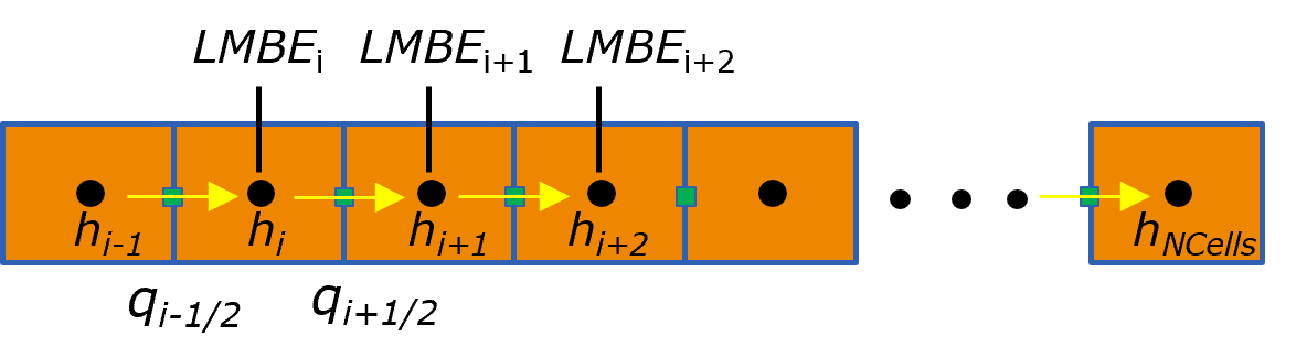
Figure 1. Conceptual 1D model illustrating the locations of the head, Darcy’s flux, and local mass balance error (LMBE) calculations.

3   Methodology

In this section, we briefly describe the analytical, FV, and PINN methods to solve Eq. 3. We consider two scenarios – homogeneous ($K$ is a constant) and heterogeneous ($K$ varies with $x$) porous media.

3.1   Analytical solution:

Considering $K$ as constant and choosing $h(x=0)=0$, and $h(x=1)=0.9$ as the Dirichlet boundary conditions, the analytical solution can be derived as follows:

$$h=-0.1x+1.$$ (5)

With $K$ varies as a function of space as $K(x)=(x+0.5)^{2}/2.25$ (a convex function), the analytical solution for the heterogeneous scenario can be derived as:

$$h=\frac{{0.075}}{{\left({x+0.5}\right)}}+{0.85}.$$ (6)

3.2   Numerical solution using finite volume:

For the homogeneous medium, the discretized forms of Eq. 3 using the two-point flux finite volume with central difference for gradient, $\frac{dh}{dx}$, are as follows

$${h_{i+1}}-2{h_{i}}+{h_{i-1}}=0,$$ (7)

while for the heterogeneous medium:

$$\left({{K_{i+1}}+{K_{i}}}\right){h_{i+1}}-\left({{K_{i+1}}+2{K_{i}}+{K_{i-1}}}\right){h_{i}}+\left({{K_{i}}+{K_{i-1}}}\right){h_{i-1}}=0.$$ (8)

Along with the boundary conditions, $h(x=0)=0$, and $h(x=1)=0.9$, the linear systems of Eqs. 7 and 8 were solved using the LU decomposition method in Scipy python package [29].

3.3   PINN solution:

The deep neural networks (DNN) approximation of groundwater heads as a function of $x$, and weights and biases ($\theta$) of a neural network is:

$$h(x)\approx\hat{h}(x;\theta).$$ (9)

DNN approximation of the governing Eq. 3 for the homogeneous case is given by

$$f(x)=\frac{\partial^{2}{h}}{\partial{x^{2}}}\approx\hat{f}(x;\theta)=\frac{{{\partial^{2}}\hat{h}(x;\theta)}}{{\partial{x^{2}}}},$$ (10)

while for the heterogeneous case is

$$f(x)=\frac{\partial}{{\partial{x}}}\left[{K\left(x\right)\frac{\partial}{{\partial x}}h(x)}\right]\approx\hat{f}(x;\theta)=\frac{\partial}{{\partial{x}}}\left[{K\left(x\right)\frac{\partial}{{\partial x}}\hat{h}(x;\theta)}\right].$$ (11)

The loss function (accounting for the losses in the PDE residual and the residual due to the boundary conditions) without training data for the above scenarios is

$$\mathcal{L}(\theta)=\frac{1}{{{N_{c}}}}{\sum\limits_{i=1}^{{N_{c}}}{\left[{\hat{f}(x_{i}^{c};\theta)}\right]}^{2}}+\frac{1}{{{N_{D}}}}{\sum\limits_{i=1}^{{N_{D}}}{\left[{\hat{h}\left({x_{i}^{D};\theta}\right)-g_{i}^{*}}\right]}^{2}}.$$ (12)

If we include training data for the heads, an additional loss term is added, and the overall loss function for the above scenarios become

$$\mathcal{L}(\theta)=\frac{1}{{{N_{c}}}}{\sum\limits_{i=1}^{{N_{c}}}{\left[{\hat{f}(x_{i}^{c};\theta)}\right]}^{2}}+\frac{1}{{{N_{D}}}}{\sum\limits_{i=1}^{{N_{D}}}{\left[{\hat{h}\left({x_{i}^{D};\theta}\right)-g_{i}^{*}}\right]}^{2}}{\rm{+}}\frac{1}{{{N_{h}}}}{\sum\limits_{i=1}^{{N_{h}}}{\left[{\hat{h}\left({x_{i}^{h};\theta}\right)-h_{i}^{*}}\right]}^{2}},$$ (13)

where, ${N_{c}}$, ${N_{D}}$, and ${N_{h}}$ represent the number of collocation points, the number of Dirichlet boundary conditions, and the number of head measurements/data, respectively. The head training data and Dirichlet boundary conditions are represented by $h^{*}$ and $g^{*}$. The first term on the right-hand side in Eq. 13 is the loss due to the PDE residual at collocation points. The second term in Eq. 13 is loss due to the Dirichlet boundary condition while the third term is the loss to match $h(x)$ to the measurements $h^{*}$. $x_{i}^{C},x_{i}^{D},x_{i}^{h}$ are the locations of the collocation points, Dirichlet, and Neumann boundaries, respectively.

The PINNs solution, $\hat{h}(x;\theta)$, is obtained by

$$\mathop{\mbox{minimize}}_{\hat{h}(x;\theta)\in\mathbb{R}^{+}}\mathcal{L}(\theta),$$ (14)

where the optimal solution is obtained by selecting the PINNs model that has minimal loss through hyperparameter tuning.

Multi-layer feed-forward DNNs [30, 31] with three hidden layers and 50 neurons per layer were used to train PINN. The hyperbolic tangent was used as the activation function because it is infinitely differentiable and facilitated for differentiating Eq. 3 twice. The remaining PINN hyperparameters are collocation points, learning rate, training data, and epoch numbers. Collocation points ($x_{i}^{C}$) in Eq. 13 are the locations in the model domain where PINN is trained for satisfying the PDE. We coincide these points with the FV cell centers for comparison its solution with analytical and numerical solutions. Training data are the observations/measurements or sampled values from an analytical solution used to train PINN. Epoch is one complete pass of the training dataset (PDE, BCs, ICs where needed, and the training data) through the optimization algorithm to train PINN. The learning rate is the step size at each epoch while PINN approaches to its minimum loss. Our codes for PINN used the DeepXDE python package [32].

3.4   Performance Metrics

In addition to the loss function, we used mean squared error ($MSE$) and correlation coefficient ($R^{2}$) for evaluating PINN models. The $MSE$ and $R^{2}$ are given by:

$$MSE=\frac{1}{n}\sum\limits_{i=1}^{n}(h_{\mathrm{a}_{i}}-h_{\mathrm{p}_{i}})^{2},$$ (15)

$$R^{2}=1-\frac{\sum\limits_{i=1}^{n}{{{\left({{h_{\mathrm{a}_{i}}}-h_{\mathrm{p}_{i}}}\right)}^{2}}}}{\sum\limits_{i=1}^{n}{{{\left({{h_{\mathrm{a}_{i}}}-{{\bar{h}}_{\mathrm{a}}}}\right)}^{2}}}},$$ (16)

where, $n$ is the number of hydraulic heads, $h_{\mathrm{a}}$ is the head from the analytical solution, $h_{\mathrm{p}}$ is the predicted head from the PINN model, and ${\bar{h}}_{\mathrm{a}}$ is the mean of heads derived from analytical solution.

4   Results

This section compares the results of the analytical, FV, and PINN methods as well as the mass balance errors associated with the FV and PINN solutions.

4.1   Homogeneous Porous Media

Two boundary conditions and 11 collocation points were used to train PINN for hydraulic head calculation. The loss function in Eq. 12 was used in this case, that is, no head data was added in the training process. PINN was trained for 20,000 epochs and the loss function fluctuated by 10 orders of magnitude even after reaching its minimum value suggesting an unsteady learning process (Figure 2a).

The minimum value for the loss function is $\approx 10^{-18}$ at 4,000 epochs. The PINN model with the minimum loss was used to calculate the hydraulic heads at each collocation point. Hydraulic heads at the same points as in PINN collocation points were also computed using analytical and FV methods. $MSE$ and $R^{2}$ between the analytical and PINN solution are $4.96\times 10^{-8}$ and $9.99\times 10^{-1}$, respectively. Such low MSE and high $R^{2}$ suggest that the PINN solution is fairly close with the analytical (Figure 2b). $MSE$ and $R^{2}$ between the analytical and FV solution are $1.68\times 10^{-32}$ ($\approx$ square of machine precision) and $1.00$, respectively.

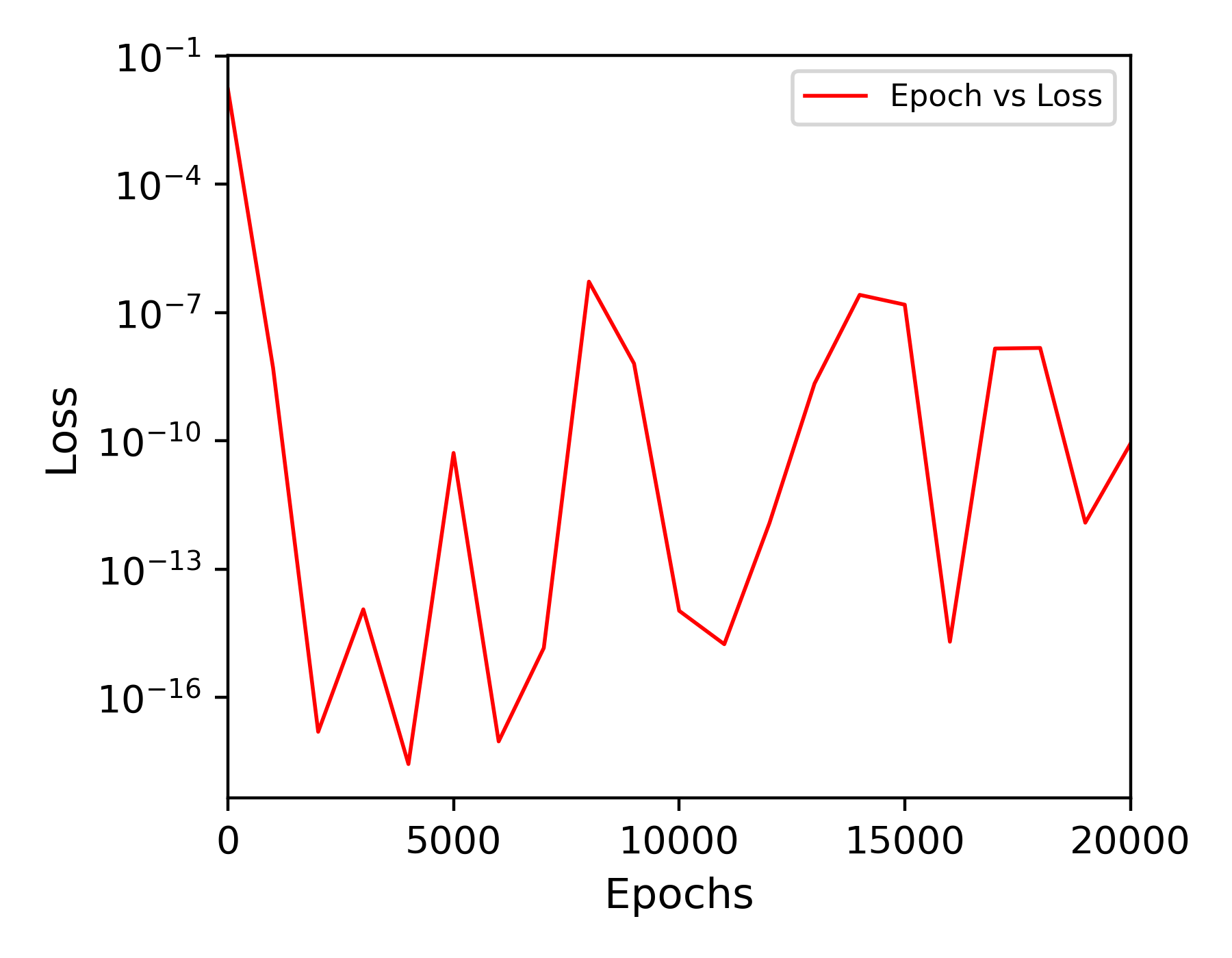
(a) Training PINN

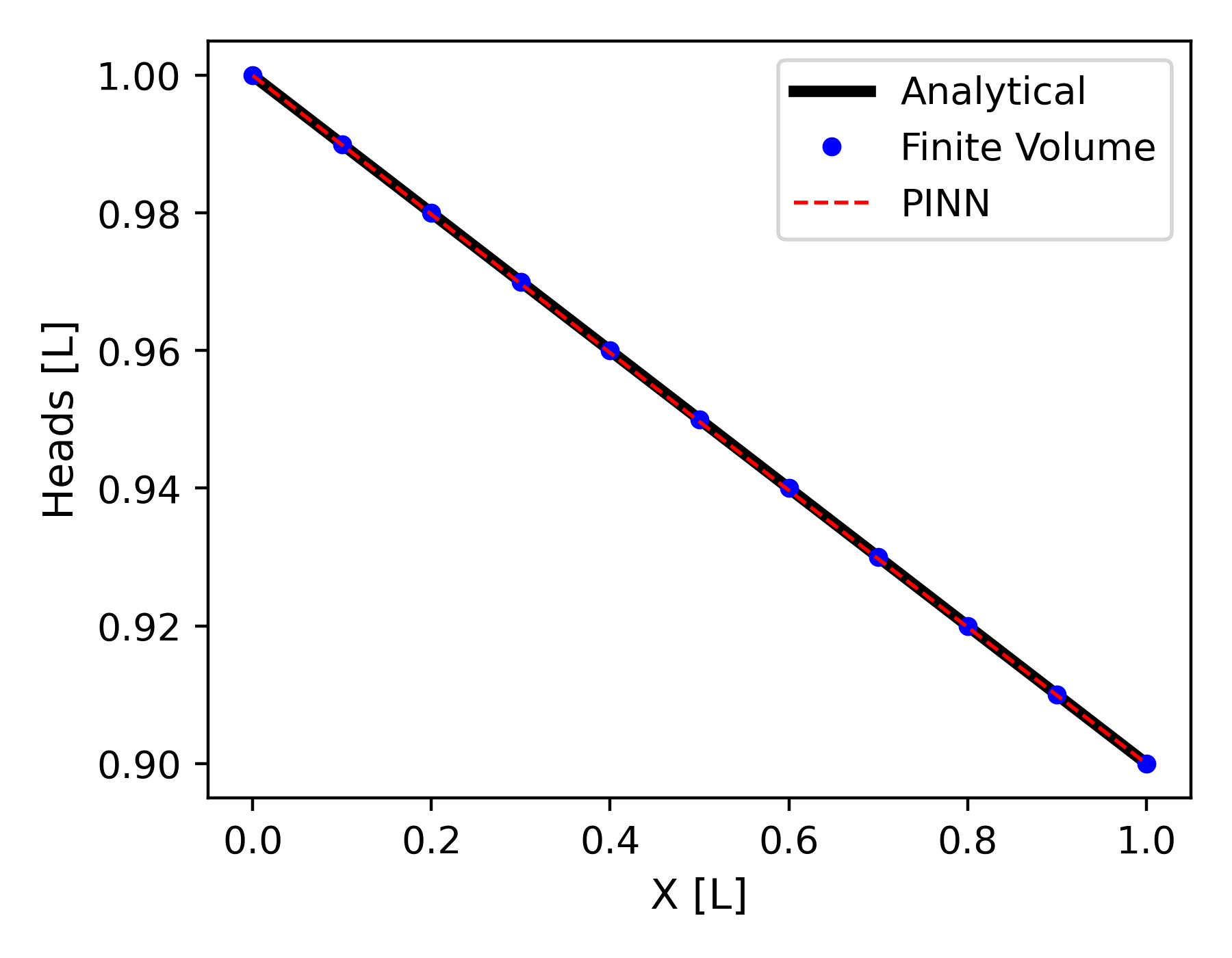
(b) Solutions for head

Figure 2. a) Epoch versus loss values during the PINN training and b) Analytical, FV, and optimal PINN solution (without any training data) for hydraulic heads for the homogeneous porous media.

Darcy’s flux is one of the indicators that represent the integrity of a numerical solution in porous media and should be constant everywhere for the homogeneous case. We computed Darcy’s fluxes on all nodes/collocation points of the model domain using Eq. 2. We found that while Darcy’s fluxes of the analytical and FV solutions are constant, they were not constant for the optimal PINN solution (Fig. 3a), and the magnitude decreases in space. However, the mean of Darcy’s fluxes computed from the optimal PINN solution was found to be the same as that of the analytical and FV solutions.

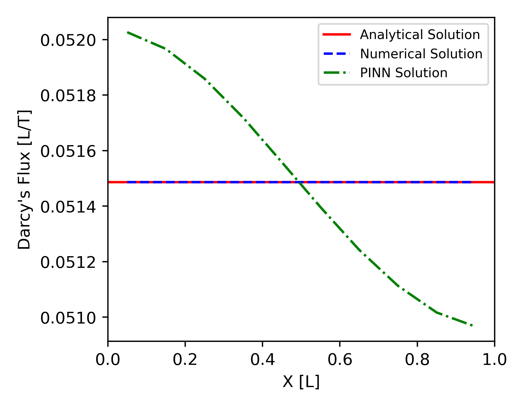
(a) Darcy’s Flux

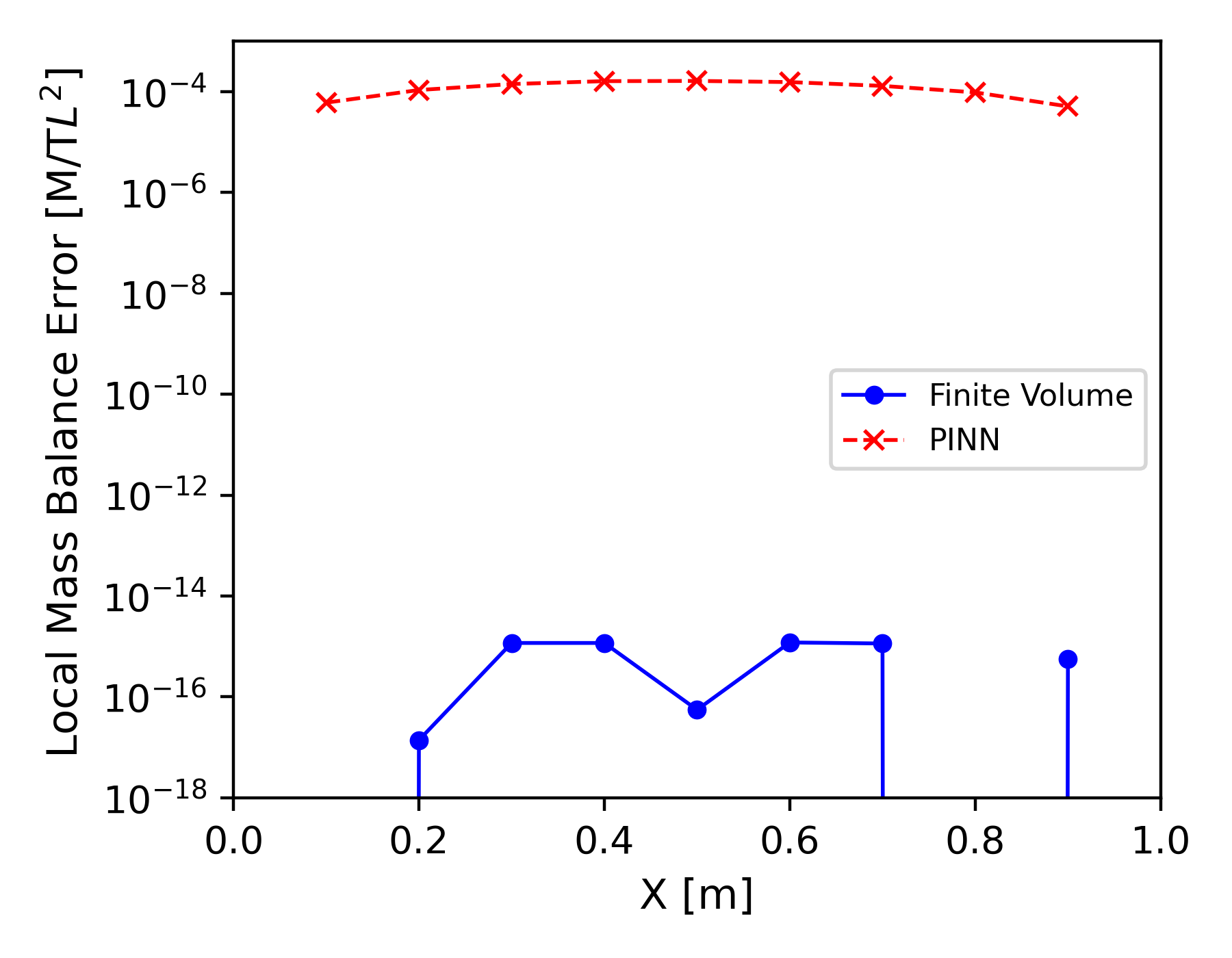
(b) Mass Balance error

Figure 3. a) Darcy’s flux calculated from the analytical, FV, and PINN solutions; and b) Mass Balance error of the FV and PINN solutions.

The mass balance in the model domain was then calculated using LMBE and GMBE equations for both FV and PINN solutions. Analytical solutions are exact solutions that do not incur round-off or numerical truncation errors. LMBE and GMBE of the analytical solutions are zero because of the exactness of the solutions; therefore, they are not discussed here. LMBEs of the FV solution vary from 0 to $\approx 10^{-15}$ or close to machine precision while they are around $\approx 10^{-4}$ for the PINN solution (Fig. 3b). The GMBE of the FV and the PINN solutions are $5.55\times 10^{-16}$ and $1.06\times 10^{-3}$, respectively. The LMBE and GMBE for PINNs are much higher than machine precision, indicating that it does not conserve mass locally and globally. A primary reason for such a large discrepancy in LMBE and GMBE between FV and PINN solutions is that FV puts a hard constraint on the balance of mass when it solves Eq. 3. Although PINN computes accurate heads, it fails to balance the mass because it tries to minimize the residual contribution from the PDE and the BCs instead of exactly setting these residuals to zero. Another potential reason for such a mismatch is the inability of the neural network to optimize its weights and biases as the loss function value gets smaller, due to the non-convex optimization nature of PINN training.

Table 1. Mass balance errors of the FV and PINN solutions for homogeneous media.

Solutions	Maximum LMBE	GMBE
FV	$1.20\times 10^{-15}$	$5.5\times 10^{-16}$
PINN	$1.62\times 10^{-4}$	$1.06\times 10^{-3}$

4.2   Heterogeneous Porous Media

The loss function in Eq. 12 was first used to train for heterogeneous porous media with boundary conditions without providing head training data. The resulting PINN head prediction was highly inaccurate compared to the analytical solution, as shown in Fig. 4 in the main text and Fig. S1 in the supplementary material. The FV solution matched well with the analytical solution. The $MSE$ and $R^{2}$ scores between PINN and analytical solutions are 0.0024 and -2.24. Here, PINN only learns the boundary condition values but fails to learn the accurate head values in the middle of the model domain.

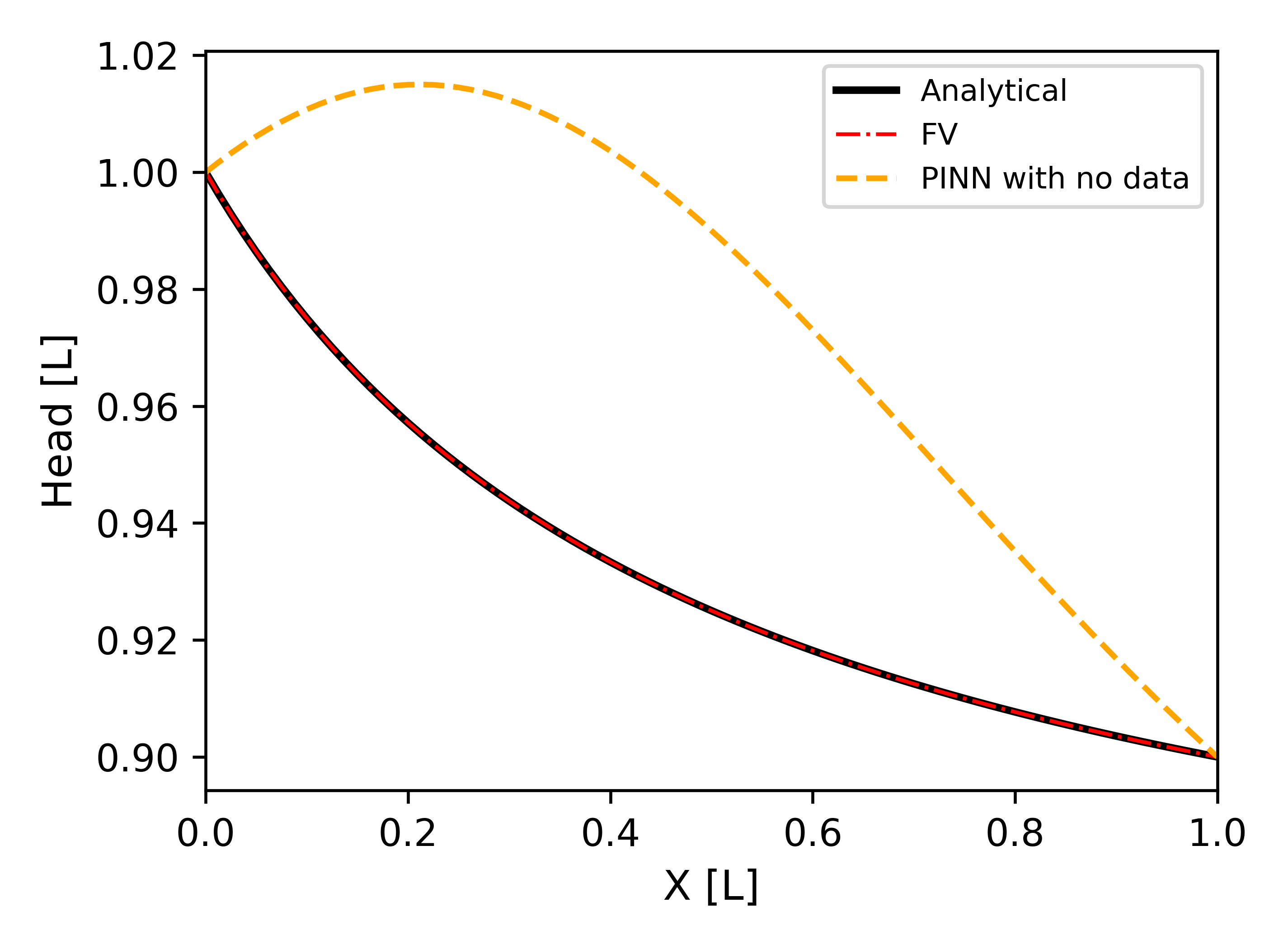
Figure 4. Hydraulic head prediction by analytical, FV, and PINN methods for the heterogeneous porous media. No training data for head was used to train the PINN solution.

4.2.1   Hyperparameter tuning

To interrogate the performance of PINN solutions, we performed hyperparameter tuning by generating an ensemble of hyperparameters. Specifically, we generated 4800 unique scenarios by varying the following hyperparameters to find an optimal PINN model for the heterogeneous case: learning rates, the number of epochs, the number of collocation points, and the number of training data points provided for the head. Table 2 lists the values chosen for these parameters.

Table 2. Hyperparameters for training PINN for the heterogeneous scenario.

Hyperparameter	Values
Learning rate	$10^{-6}$, $10^{-5}$, $10^{-4}$, $10^{-3}$, $10^{-2}$, $10^{-1}$
Number of epochs	$(10,20,30,40,50,60,70,80,90,100)\times 10^{3}$
Number of collocation points	11, 21, 41, 81, 161
Number of training data points	0, 1, 2, 3, 4, 5, 6, 7, 8, 9, 10, 20, 40, 60, 100, 160

We considered two metrics for finding an optimal PINN model: the minimum loss of the PINN training and the minimum MSE of the head between PINN and analytical solutions. The minimum loss provides the best solution for the training process but does not necessarily generate the best model. For instance, a significantly low minimum loss may generate a PINN model, which provides a high MSE. Therefore, we need a model which also provides a low MSE value.

Next, we describe how each PINN hyperparameter affects the PINN solution and how we found an optimal PINN model. Figure 5 shows minimum loss versus MSE values for each of the hyperparameters. Scenarios on the left side of the boxed portion have low minimum loss but high MSE, while scenarios in the right portion have high scores for both metrics. However, scenarios in the boxed portion have low values for both metrics. The red box in Fig. 5 has the following threshold: mininum loss $\in[10^{-7},10^{-16}]$ and MSE $\in[10^{-7},10^{-14}]$.

Figure 5(a) demonstrates that large learning rates (¿$10^{-2}$) prominently provide low minimum loss but high MSE. This is reasonable because a large learning rate quickly finds accurate values for boundary conditions and training data without learning the PDE solution accurately. A low learning rate allows us to search multiple local minima within the non-convex loss function resulting in high values for both metrics. However, many scenarios for the learning rates ranging from $10^{-5}$ to $10^{-2}$ provide low scores for both metrics suggesting learning rates within this range will likely generate accurate PINN models.

The number of training data points provided has relatively a higher control on minimum loss and MSE (Figure 5c). Generally, more training data points generate better models. Note that a large number of training data may also generate wrong PINN models if learning rates and epoch numbers are outside the ranges shown in the red box. Lower training data points may provide an accurate model if learning rates and epoch numbers are within the threshold box. Our detailed analysis indicates that the number of training data >20 will likely generate accurate PINN models.

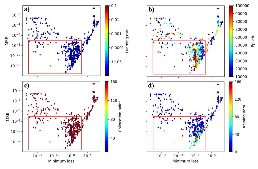
Figure 5. Minimum loss and mean squared error for 4800 hyperparameter scenarios. The hyperparameters considered were: a) the learning rate, b) the number of epochs, c) the number of collocation points, and d) the number of training data points. The scenarios in the red box highlight the cases where minimum loss and MSE are low.

Although hyperparameter tuning is computationally expensive, finding the optimal model for a comparison study with FV’s solution is necessary. The optimal model falls in the boxed portion, where minimum loss and minimum MSE are $1.69\times 10^{-8}$ and $1.00\times 10^{-16}$, respectively. The optimal model’s corresponding learning rate, epoch number, collocation point, and training data are $10^{-4}$, 70000, 81, and 40, respectively. Hydraulic head prediction by analytical, FV, and PINN with 40 training data points are consistent (Figure 6). The $MSE$ and $R^{2}$ between hydraulic head prediction by analytical and optimal PINN with 40 training data points are 0.0 and 1, respectively.

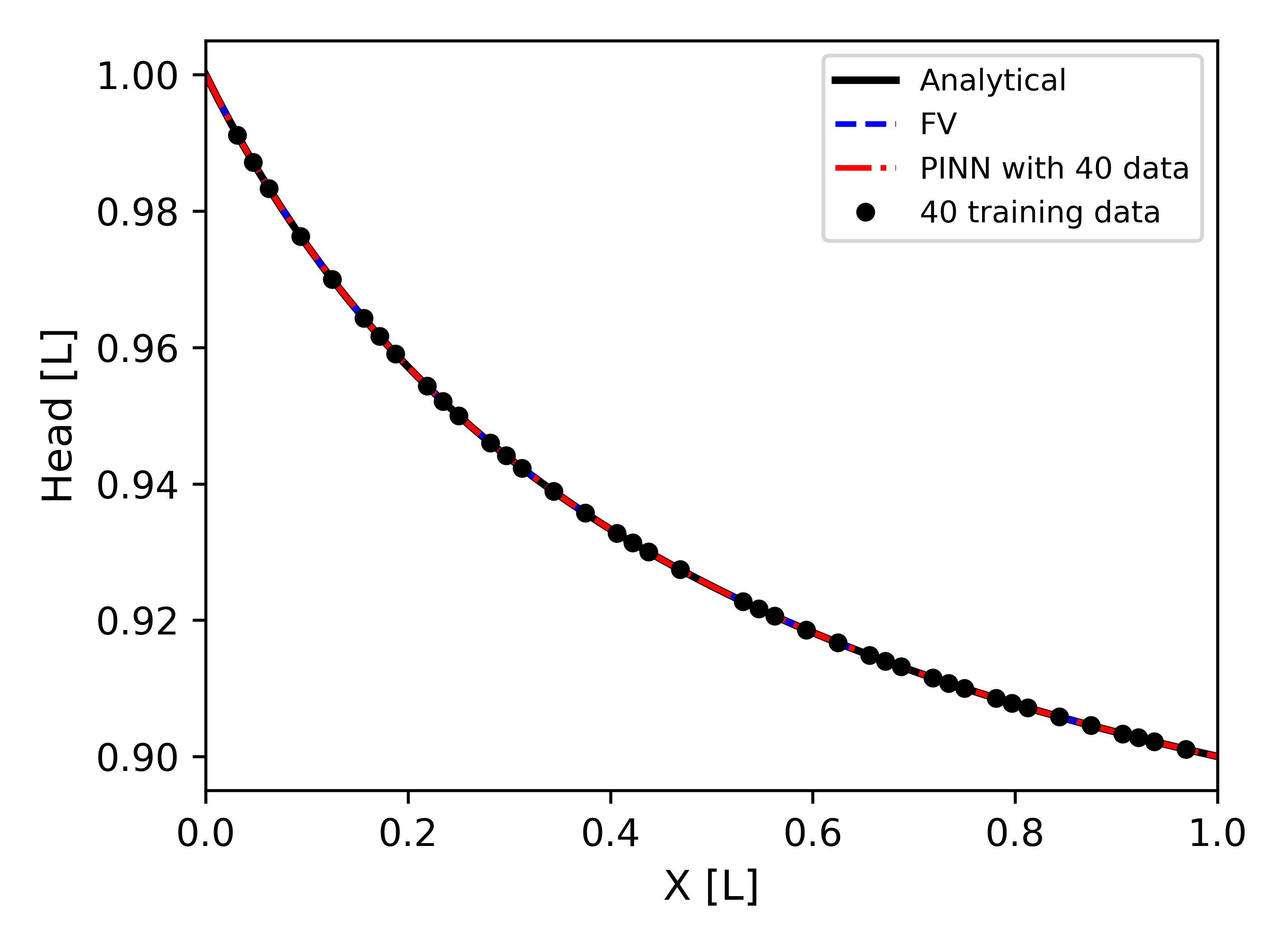
Figure 6. Hydraulic head prediction by analytical, FV, and optimal PINN with 40 training data for the heterogeneous porous media.

We computed Darcy’s fluxes on all nodes/collocation points of the model domain using Eq. 2. We found that while the Darcy’s fluxes of the analytical and FV solutions are constant, they were not constant for the PINN solution (Figure 7a) and the magnitude decreases in space. However, the mean of Darcy’s fluxes from the PINN solution was same as that of the analytical and FV solutions. In both cases, hydraulic head predictions are accurate, but Darcy’s fluxes are not accurate compared to its counterpart FV solution. Figures S2 to S4 in supplementary material show convergence studies for both FV and PINN solutions. This includes progressively adding analytical solution data at collocation points to improve PINN’s training. The figures in S2-S4 show that mass balance errors are still significant, with minimal improvements even when more data is added.

The maximum LMBE of the FV and the optimal PINN solutions are $2.44\times 10^{-7}$ and $3.13\times 10^{-5}$, respectively (Figure 7a and Table 3). The LMBE of the optimal PINN solution is two orders of magnitude higher than that of the FV solution. The GMBE of the FV and the optimal PINN solutions are $4.53\times 10^{-6}$ and $6.92\times 10^{-6}$, respectively. The magnitudes GMBE of PINN and FV are close suggesting the comparable performance of optimal PINN with FV.

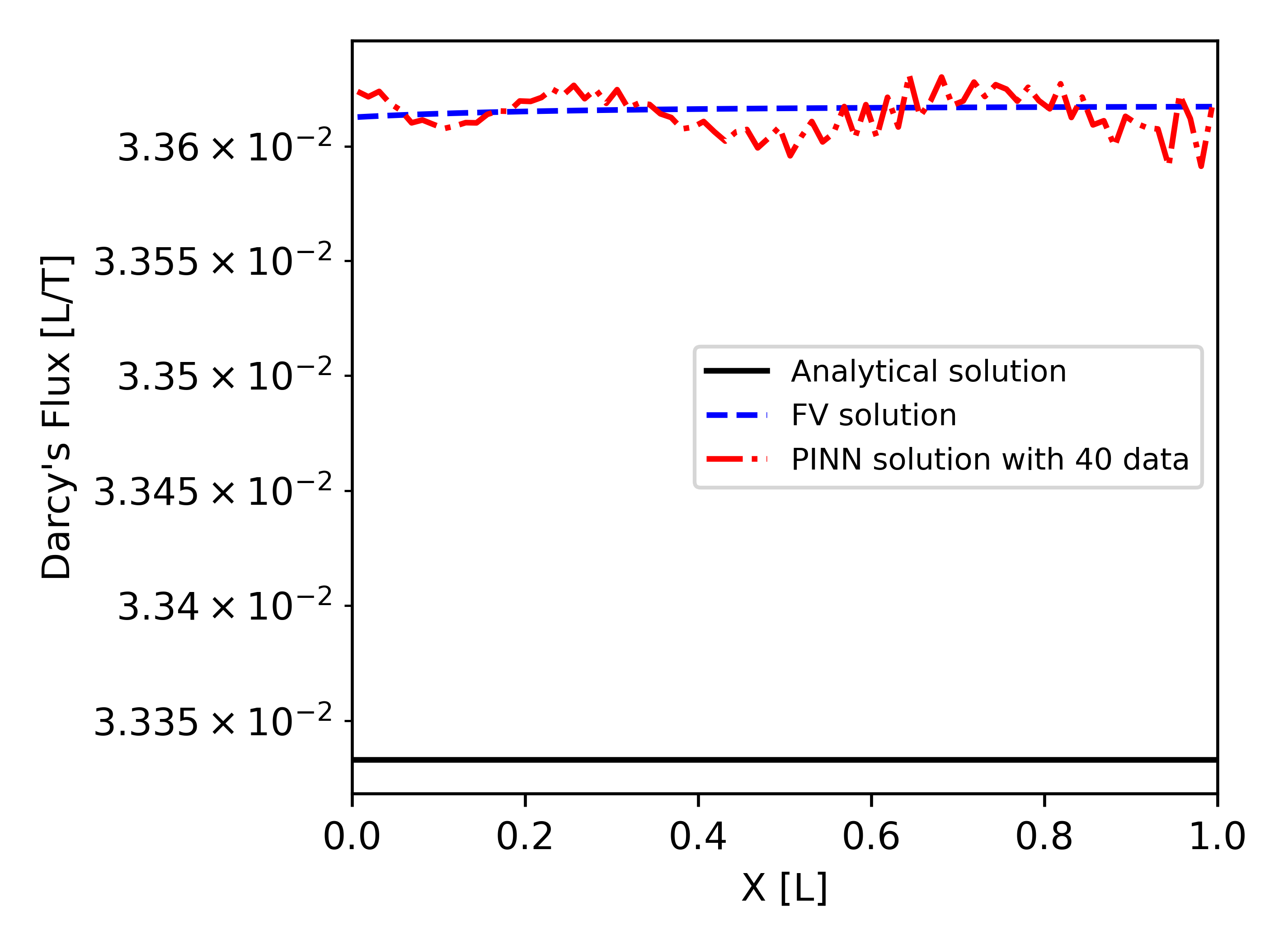
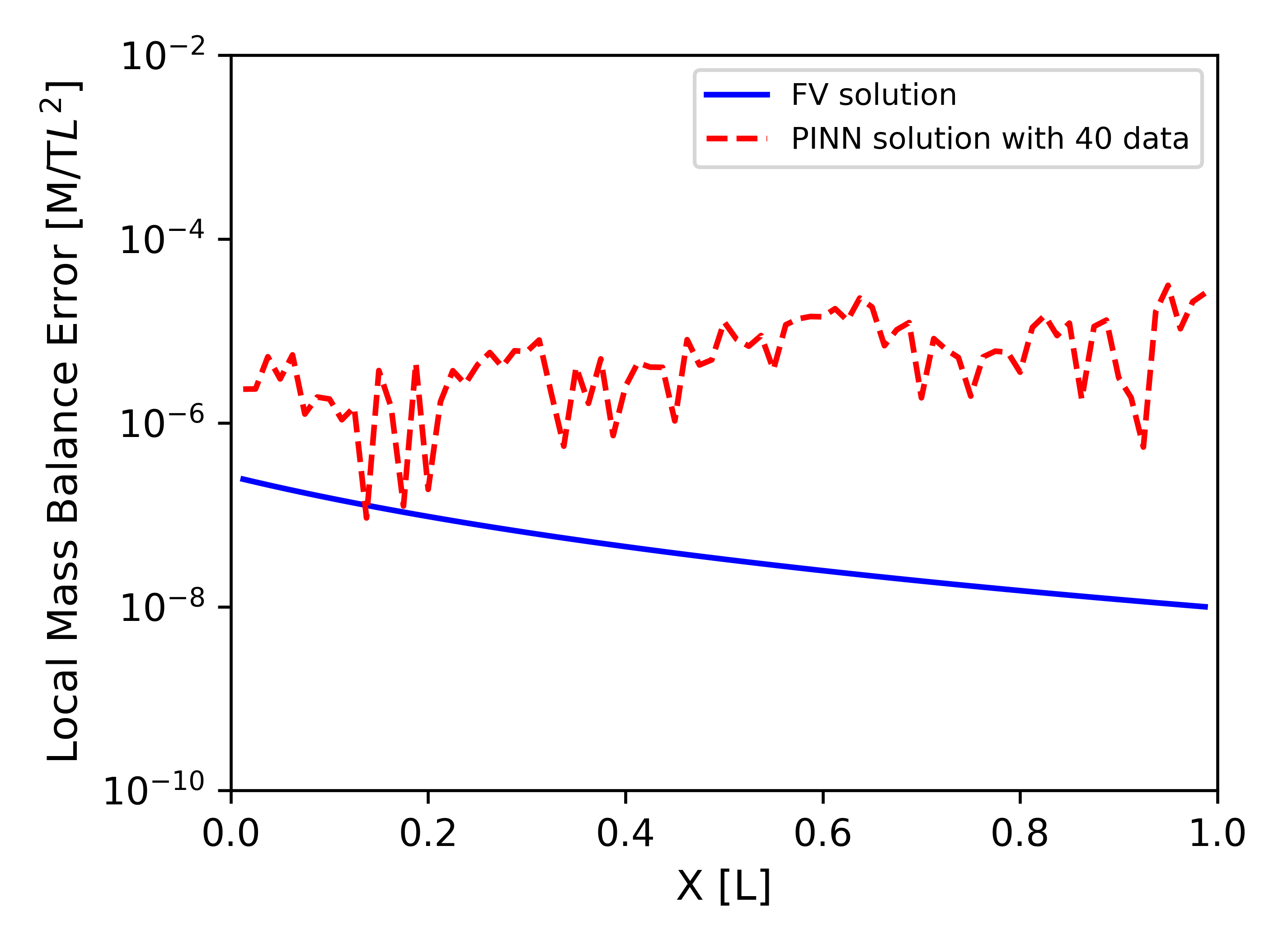
Figure 7. a) Darcy’s flux was calculated from the analytical, FV, and optimal PINN solution for the heterogeneous porous media, and b) Mass Balance error with the FV and optimal PINN solution for 81 collocation points and 40 data.

Table 3. Mass balance errors of the FV and optimal PINN solution for the heterogeneous case.

Method	Maximum LMBE	GMBE
FV	$2.44\times 10^{-7}$	$4.53\times 10^{-6}$
PINN	$3.13\times 10^{-5}$	$6.92\times 10^{-6}$

5   Conclusions

PINN is an alternative approach to numerical solutions solving physical problems, which a partial differential equation can describe. We investigated whether PINN conserved mass and compared its performance with the FV method. For this purpose, we solved a steady-state 1D groundwater flow equation for predicting hydraulic heads using analytical, FV, and PINN methods for both homogeneous and heterogeneous media. The accuracy of the PINN model was computed using $MSE$ and $R^{2}$ scores between hydraulic head prediction by analytical and PINN methods. Next, the integrity of PINN models was investigated using Darcy’s flux, LMBE, and GMBE. Finally, we compared its performance with the FV method.

For the homogeneous media case, $MSE$ and $R^{2}$ scores are 0.0 and 1.0, respectively, suggesting accurate prediction by PINN. Darcy’s flux is not constant as it is for the analytical and FV methods. The LMBE is close to zero for FV solution while it is $10^{-6}$ for PINN. The GMBE of PINN solution is 10 magnitudes higher than FV solution. Such a large discrepancy is due to how PINN finds its solution by softly enforcing the PDE constraints.

For the heterogeneous media case, we performed extensive hyperparameter tuning to find an optimal PINN and compare it with the FV solution. We found that without adding training data points, PINN fails to predict accurate hydraulic heads with only boundary conditions, let alone Darcy’s flux, LMBE, and GMBE. We found that hydraulic head prediction by analytical, FV, and optimal PINN with 40 training data are consistent. One needs to provide extensive training data points for training PINN to have an LMBE closer to FV. These findings shed light on the limitations of PINNs to applications where conserving mass locally is essential.

Abbreviations

• PINN: Physics-Informed Neural Networks

• PDE: Partial Differential Equations

• ODE: Ordinary Differential Equations

• FV: Finite Volume

• DNN: Deep Neural Networks

• MSE: Mean Squared Error

• LMF: Local Mass Flux

• LMBE: Local Mass Balance Error

• GMBE: Global Mass Balance Error

• CP: Collocation Points

• TD: Training Data

Conflict of Interest

The authors declare that they do not have any conflicts of interest.

Data Availability

The codes and the data used in the paper are available at https://gitlab.com/bulbulahmmed/mass_balance_of_pinn.

Appendix

The supplementary material contains figures on the training of PINNs, mass balance errors, and PDE residual with and without data. These figures are provided in a separate file.

References

- [1] W. Guo, “Analytical solution of transient radial air flow to an extraction well,” Journal of Hydrology, vol. 194, no. 1, pp. 1–14, 1997.
- [2] S. V. Meleshko, Methods for constructing exact solutions of partial differential equations: mathematical and analytical techniques with applications to engineering. Springer, 2005.
- [3] E. J. Wexler, Analytical solutions for one-, two-, and three-dimensional solute transport in ground-water systems with uniform flow. US Government Printing Office, 1992.
- [4] L. F. Richardson, “IX. The approximate arithmetical solution by finite differences of physical problems involving differential equations, with an application to the stresses in a masonry dam,” Philosophical Transactions of the Royal Society of London. Series A, Containing Papers of a Mathematical or Physical Character, vol. 210, no. 459-470, pp. 307–357, 1911.
- [5] J. Peiró and S. Sherwin, “Finite difference, finite element and finite volume methods for partial differential equations,” Handbook of Materials Modeling: Methods, pp. 2415–2446, 2005.
- [6] R. J. LeVeque, Finite volume methods for hyperbolic problems, vol. 31. Cambridge university press, 2002.
- [7] F. Moukalled, L. Mangani, M. Darwish, F. Moukalled, L. Mangani, and M. Darwish, The finite volume method. Springer, 2016.
- [8] C. Johnson, Numerical solution of partial differential equations by the finite element method. Courier Corporation, 2012.
- [9] I. E. Lagaris, A. Likasa, and D. I. Fotiadi, “Artifial Neural Networks for Solving Ordinary and,” 1997.
- [10] I. E. Lagaris, A. C. Likas, and D. G. Papageorgiou, “Neural-network methods for boundary value problems with irregular boundaries,” IEEE Transactions on Neural Networks, vol. 11, pp. 1041–1049, 9 2000.
- [11] M. Raissi, P. Perdikaris, and G. E. Karniadakis, “Physics Informed Deep Learning (Part II): Data-driven Discovery of Nonlinear Partial Differential Equations,” 11 2017.
- [12] D. Chen, X. Gao, C. Xu, S. Wang, S. Chen, J. Fang, and Z. Wang, “FlowDNN: a physics-informed deep neural network for fast and accurate flow prediction,” Frontiers of Information Technology and Electronic Engineering, vol. 23, pp. 207–219, 2 2022.
- [13] L. Lu, X. Meng, Z. Mao, and G. E. Karniadakis, “DeepXDE: A deep learning library for solving differential equations,” 7 2019.
- [14] Y. Chen, L. Lu, G. E. Karniadakis, and L. D. Negro, “Physics-informed neural networks for inverse problems in nano-optics and metamaterials,” 12 2019.
- [15] J. Han, A. Jentzen, and W. E, “Solving high-dimensional partial differential equations using deep learning,” 7 2017.
- [16] S. Kakkar, “Physics-informed deep learning for computational fluid flow analysis coupling of physics-informed neural networks and autoencoders for aerodynamic flow predictions on variable geometries,” 2022.
- [17] Z. Liu, Y. Yang, and Q. Cai, “Solving Differential Equation with Constrained Multilayer Feedforward Network,” 4 2019.
- [18] S. Rezaei, A. Harandi, A. Moeineddin, B. Bai-Xiang Xu, and S. Reese, “A mixed formulation for physics-informed neural networks as a potential solver for engineering problems in heterogeneous domains: comparison with finite element method,” 6 2022.
- [19] H. Eivazi, M. Tahani, P. Schlatter, and R. Vinuesa, “Physics-informed neural networks for solving reynolds-averaged navier-stokes equations,” Physics of Fluids, vol. 34, 7 2022.
- [20] A. Kashefi and T. Mukerji, “Physics-informed pointnet: A deep learning solver for steady-state incompressible flows and thermal fields on multiple sets of irregular geometries,” 2 2022.
- [21] M. Raissi, P. Perdikaris, and G. E. Karniadakis, “Physics-informed neural networks: A deep learning framework for solving forward and inverse problems involving nonlinear partial differential equations,” Journal of Computational Physics, vol. 378, pp. 686–707, 2 2019.
- [22] F. Giampaolo, M. D. Rosa, P. Qi, S. Izzo, and S. Cuomo, “Physics-informed neural networks approach for 1d and 2d gray-scott systems,” Advanced Modeling and Simulation in Engineering Sciences, vol. 9, 12 2022.
- [23] R. Rodriguez-Torrado, P. Ruiz, L. Cueto-Felgueroso, M. C. Green, T. Friesen, S. Matringe, and J. Togelius, “Physics-informed attention-based neural network for hyperbolic partial differential equations: application to the buckley–leverett problem,” Scientific Reports, vol. 12, 12 2022.
- [24] A. D. Jagtap, E. Kharazmi, and G. E. Karniadakis, “Conservative physics-informed neural networks on discrete domains for conservation laws: Applications to forward and inverse problems,” Computer Methods in Applied Mechanics and Engineering, vol. 365, p. 113028, 2020.
- [25] P. Chuang and L. A. Barba, “Experience report of physics-informed neural networks in fluid simulations: pitfalls and frustration,” 2022.
- [26] T. Grossmann, U. Komorowska, J. Latz, and C. Schönlieb, “Can physics-informed neural networks beat the finite element method?,” arXiv preprint arXiv:2302.04107, 2023.
- [27] S. Cuomo, V. S. di Cola, F. Giampaolo, G. Rozza, M. Raissi, and F. Piccialli, “Scientific Machine Learning through Physics-Informed Neural Networks: Where we are and What’s next,” 1 2022.
- [28] X. Huang and T. Alkhalifah, “Efficient physics-informed neural networks using hash encoding,” arXiv preprint arXiv:2302.13397, 2023.
- [29] P. Virtanen, R. Gommers, T. E. Oliphant, M. Haberland, T. Reddy, D. Cournapeau, E. Burovski, P. Peterson, W. Weckesser, J. Bright, et al., “Scipy 1.0: fundamental algorithms for scientific computing in python,” Nature methods, vol. 17, no. 3, pp. 261–272, 2020.
- [30] G. Bebis and M. Georgiopoulos, “Feed-forward neural networks,” IEEE Potentials, vol. 13, no. 4, pp. 27–31, 1994.
- [31] D. Svozil, V. Vladimir KvasniEka, and J. JiE Pospichal, “Introduction to multi-layer feed-forward neural networks,” Chemometrics and Intelligent Laboratory Systems, vol. 39, pp. 43–62, 1997. Publisher: Elsevier.
- [32] L. Lu, X. Meng, Z. Mao, and G. E. Karniadakis, “Deepxde: A deep learning library for solving differential equations,” SIAM review, vol. 63, no. 1, pp. 208–228, 2021.