Non-equilibrium dynamics of dipole-charged fields in the Proca theory

Abstract

We discuss the dynamics of field configurations encoded in the certain class of electric (magnetic) dipole-charged states in the Proca theory of the real massive vector field. We construct such states so as to ensure that the long distance structure of the mean electromagnetic field in them is initially set by the formula describing the electromagnetic field of the electric (magnetic) dipole. We analyze then how such a mean electromagnetic field evolves in time. We find that far away from the center of the initial field configuration, the long range component of the mean electromagnetic field harmonically oscillates, which leads to the phenomenon of the periodic oscillations of the electric (magnetic) dipole moment. We also find that near the center of the initial field configuration, the mean electromagnetic field escapes from its initial arrangement and a spherical shock wave propagating with the speed of light appears in the studied system. A curious configuration of the axisymmetric mean electric field is found to accompany the mean magnetic field in magnetic dipole-charged states.

I Introduction

The Proca theory studied in this work is defined by the following Lagrangian density Greiner and Reinhardt (1996); Chen et al. (2018); Weinberg (2010)

$${\cal L}=-\frac{1}{4}(\partial_{\mu}V_{\nu}-\partial_{\nu}V_{\mu})^{2}+\frac{m^{2}}{2}(V_{\mu})^{2},$$ (1)

where $V$ is the vector field operator and $m$ is the mass of the vector boson that it describes (see Appendix A for our conventions and Goldhaber and Nieto (2010); Tu et al. (2005) for the general discussion of the Proca theory in the context of massive photon electrodynamics). Such a theory differs from the Maxwell theory by the mass term, which leads to the non-vanishing energy of small momentum excitations

$$\varepsilon_{k}=\sqrt{m^{2}+|{\bm{k}}|^{2}}=m+O\left(|{\bm{k}}|^{2}\right)\ \text{for}\ {\bm{k}}\to\bm{0}.$$ (2)

This simple observation suggests that the mass $m$ should play a role in the large-distance dynamics of the electromagnetic field of the Proca theory, which is represented by the operators $\bm{E}=-\partial_{0}\bm{V}-{\bm{\nabla}}V^{0}$ and $\bm{B}={\bm{\nabla}}\times\bm{V}$. This expectation was discussed in our recent work BDP , which we briefly summarize below to set the stage for the presentation of our follow up results.

Namely, we studied the dynamics of the mean electric field in the certain class of charged states in the Proca theory BDP . The hallmark feature of such states was the non-zero expectation value of the charge operator

$$Q(t)=\int d^{3}\mkern-1.5muy\,\text{div}\bm{E}(t,{\bm{y}})$$ (3)

in them. This was analyzed in the following setup (Fig. 1). At some time, say $t=0$, we assumed that the system was in the state, where the mean electric field was asymptotically given by the Coulomb formula

$$\left.\langle\bm{E}\rangle\right|_{t=0}\propto\frac{\bm{r}}{4\pi r^{3}}\ \text{for}\ r=|\bm{r}|\to\infty.$$ (4)

For $t>0$, the mean electric field underwent non-equilibrium dynamics because there was no external source generating field (4) in the studied system. This lead to the appearance of the shock wave that was localized on the expanding sphere of radius $t$ (the mean electric field was weakly discontinuous at $r=t$ Rem (a)). Space in the considered problem was split into two regions. The one that had already been swept by the shock wave ($r<t$) and the one where the shock wave had not yet arrived ($r>t$). In the former region, the dynamics of the mean electric field was non-universal because it depended on the short distance properties of such a field at $t=0$, which could be chosen in different ways Rem (b). In the latter region, the universal feature of the mean electric field was identified. Namely, the periodically oscillating Coulomb field,

$$\propto\frac{\bm{r}}{4\pi r^{3}}\cos(mt),$$ (5)

dominated the long distance behavior of the mean electric field in the studied states. This result explained the phenomenon of periodic charge oscillations in the Proca theory BDP ; Rem (c). A similar phenomenon was mentioned in a different physical context in Hertzberg and Jain (2020).

The problem explored in this work is related to the one, which has just been explained. Namely, we will discuss the dynamics of the mean electromagnetic field in dipole-charged states in the Proca theory, where the asymptotic form of such a field is initially given by the formula describing the electromagnetic field of either the electric or magnetic dipole. Such a problem, to the best of our knowledge, has not been studied before.

The outline of this paper is the following. Basic facts concerning the Proca theory as well as the technical details related to the construction of the dipole-charged states are presented in Sec. II and Appendix B. The magnetic and electric dipole-charged states are discussed in Secs. III and IV, respectively. It is shown there how one may construct them, so that they represent finite-energy field configurations, and then the dynamics of the mean electromagnetic field in such states is analyzed. The summary of our work is presented in Sec. V, whereas our conventions are listed in Appendix A.

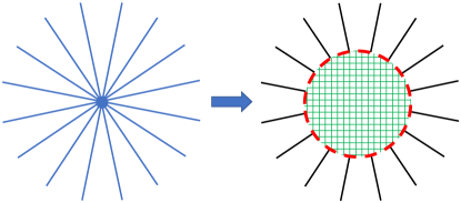
Figure 1: Schematic illustration of the non-equilibrium dynamics of the mean electric field in states discussed in BDP . The plots depict the initial mean electric field, approximately given by the Coulomb formula, and its non-equilibrium configuration after some time evolution. The dashed red line shows the shock wave front that is localized on a sphere, whereas the crossed lines show the region of space that has already been swept by the shock wave. The mean electric field also evolves outside the shock wave sphere, where it is dominated by the periodic oscillations of its Coulomb component. This is illustrated by the different colors of the field lines in the two plots.

II Basic equations

The vector field operator of the Proca theory can be written as Greiner and Reinhardt (1996)

$$V^{\mu}(x)=\int\frac{d^{3}\mkern-1.5muk\,}{(2\pi)^{3/2}}\frac{1}{\sqrt{2\varepsilon_{k}}}\\ \sum_{\sigma=1}^{3}\eta^{\mu}({\bm{k}},\sigma)a_{{\bm{k}}\sigma}\exp(-\mathrm{i}k\cdot x)+\text{h.c.},$$ (6a)

where the commutators of creation and annihilation operators are ($$\sigma,\sigma^{\prime}=1,2,3$$)

$$[a_{{\bm{k}}\sigma},a^{\dagger}_{{\bm{k}}^{\prime}\sigma^{\prime}}]=\delta_{\sigma\sigma^{\prime}}\delta({\bm{k}}-{\bm{k}}^{\prime}),\ [a_{{\bm{k}}\sigma},a_{{\bm{k}}^{\prime}\sigma^{\prime}}]=0,$$ (6b)

the transverse polarization $$4 i,j=1,2$$-vectors satisfy ()

$$\eta({\bm{k}},i)=\left(0,{\bm{\eta}}({\bm{k}},i)\right),\ {\bm{\eta}}({\bm{k}},i)\in\mathbbm{R}^{3},$$ (6c)

$${\bm{\eta}}({\bm{k}},i)\cdot{\bm{k}}=0,\ {\bm{\eta}}({\bm{k}},i)\cdot{\bm{\eta}}({\bm{k}},j)=\delta_{ij},$$ (6d)

the longitudinal polarization $$4$$-vector is given by

$$\eta({\bm{k}},3)=\left(\frac{\omega_{k}}{m},\frac{\varepsilon_{k}}{m}{\hat{\bm{k}}}\right),\ {\hat{\bm{k}}}={\bm{k}}/\omega_{k},$$ (6e)

the operators $a_{{\bm{k}}\sigma}$ annihilate the vacuum state $|0\rangle$, $\omega_{k}=|{\bm{k}}|$, and $k^{0}=\varepsilon_{k}$ is tacitly assumed in all our $d^{3}k$ integrals in which the integrand depends on $k^{0}$.

The electric and magnetic field operators of the Proca theory can be computed out of (6e) and they read

$$\bm{E}(x)=\mathrm{i}\int\frac{d^{3}\mkern-1.5muk\,}{(2\pi)^{3/2}}\sqrt{\frac{\varepsilon_{k}}{2}}\sum_{\sigma=1}^{3}\left(1-\frac{\omega_{k}^{2}}{\varepsilon_{k}^{2}}\delta_{\sigma 3}\right)\\ {\bm{\eta}}({\bm{k}},\sigma)a_{{\bm{k}}\sigma}\exp(-\mathrm{i}k\cdot x)+\text{h.c.},$$ (7)

$$\bm{B}(x)=\mathrm{i}\int\frac{d^{3}\mkern-1.5muk\,}{(2\pi)^{3/2}}\frac{1}{\sqrt{2\varepsilon_{k}}}\sum_{\sigma=1}^{2}{\bm{k}}\times{\bm{\eta}}({\bm{k}},\sigma)\\ a_{{\bm{k}}\sigma}\exp(-\mathrm{i}k\cdot x)+\text{h.c.}$$ (8)

The quantum states of interest will be considered in the following form

$$|\psi(\bm{x})\rangle=\left[\alpha-\frac{\mathrm{i}}{\alpha}\chi(\bm{x})\right]|0\rangle,$$ (9)

where $\chi(\bm{x})=\chi^{\dagger}(\bm{x})$ is linear in creation and annihilation operators while $\alpha\in\mathbbm{R}\setminus\{0\}$ is constrained by the requirement of $\langle\psi(\bm{x})|\psi(\bm{x})\rangle=1$, which leads to

$$1=\alpha^{2}+\frac{1}{\alpha^{2}}\langle 0|\chi(\bm{x})\chi(\bm{x})|0\rangle.$$ (10)

Besides the normalizability of the wave-function, we will also require that

$${\cal H}=\langle\psi(\bm{x})|H|\psi(\bm{x})\rangle=\frac{1}{\alpha^{2}}\langle 0|\chi(\bm{x})[H,\chi(\bm{x})]|0\rangle<\infty,$$ (11)

where $H$ is the Hamiltonian of the Proca theory Greiner and Reinhardt (1996)

$$H=\int d^{3}\mkern-1.5muk\,\varepsilon_{k}\sum_{\sigma=1}^{3}a_{{\bm{k}}\sigma}^{\dagger}a_{{\bm{k}}\sigma}.$$ (12)

The mean values of operators in state (9) will be computed via

$$\langle O(t,\bm{r})\rangle=\langle\psi(\bm{x})|O(t,{\bm{y}})|\psi(\bm{x})\rangle=-\mathrm{i}[O(t,{\bm{y}}),\chi(\bm{x})],$$ (13)

where $\bm{r}={\bm{y}}-\bm{x}$. The time $t>0$ will be assumed in inequalities involving $t$ and the frequently appearing equation $r=t$. The operator $\chi(\bm{x})$ will be chosen such that $\alpha$ and $\cal H$ will be independent of $\bm{x}$ and (13) will be the function of $\bm{r}$, which the above notation suggests.

We introduce

$$\phi_{\gamma}(t,r)=\frac{1}{2\pi^{2}}\int_{0}^{\infty}d\omega_{k}\left(\frac{m}{\varepsilon_{k}}\right)^{\gamma}{\rm j}_{0}(\omega_{k}r)\cos(\varepsilon_{k}t),$$ (14)

where $\gamma$ is a positive even number and ${\rm j}_{n}$ is the spherical Bessel function of the first kind of order $n$. Function (14), originally considered in BDP , will appear in the subsequent sections. For the present work, we need to know the following facts.

First, for $r\geq t$

$$\phi_{\gamma}(t,r)=\frac{\cos(mt)-P_{\gamma}(mr,mt)\exp(-mr)}{4\pi r},$$ (15)

where $P_{2}(a,b)=1$ while $P_{4,6,8,\cdots}(a,b)$ can be obtained via

$$P_{\gamma}(a,b)=-\int_{0}^{b}dy\int_{0}^{y}dxP_{\gamma-2}(a,x)\\ +P_{\gamma-2}(a,0)+\frac{a}{\gamma-2}\left(1-\frac{d}{da}\right)P_{\gamma-2}(a,0).$$ (16)

Such a recursive formula has been derived in Appendix B and it leads to

$$P_{4}(a,b)=1+\frac{a}{2}-\frac{b^{2}}{2},$$ (17)

$$P_{6}(a,b)=1+\frac{5a}{8}+\frac{a^{2}}{8}-\frac{b^{2}}{2}-\frac{ab^{2}}{4}+\frac{b^{4}}{24},$$ (18)

etc.

Second, in the $0<r<t$ region, we are unaware how $\phi_{\gamma}(t,r)$ can be analytically evaluated. However, it was shown in BDP that in such a region of space, (14) for $\gamma=2$ can be rewritten into the form that can be more conveniently analyzed.

Third, it was proved in BDP that $\phi_{\gamma}(t,r)$ and its derivatives up to order $\gamma-2$ are continuous for all $r,t>0$ (circumstantial evidence presented in BDP suggests that the same is true for the derivatives of order $\gamma-1$). It was also proved there that at least some derivatives of $\phi_{\gamma}(t,r)$ of order $\gamma$ are discontinuous at $r=t$, thereby $\phi_{\gamma}(t,r)$ is non-analytic.

III Magnetic dipole-charged states

The states studied here will be constructed such that $\langle\bm{E}(0,\bm{r})\rangle=\bm{0}$ for $r\geq 0$ and

$$\langle\bm{B}(0,\bm{r})\rangle=\frac{3({\bm{\mu}}\cdot{\hat{\bm{r}}}){\hat{\bm{r}}}-{\bm{\mu}}}{4\pi r^{3}}$$ (19)

for $r\to\infty$, where ${\bm{\mu}}$ is the magnetic dipole moment and ${\hat{\bm{r}}}=\bm{r}/r$.

To proceed, we combine the following ansatz

$$\chi(\bm{x})=\int\frac{d^{3}\mkern-1.5muk\,}{(2\pi)^{3/2}}\sum_{\sigma=1}^{2}g_{\sigma}({\bm{k}})a_{{\bm{k}}\sigma}\exp(\mathrm{i}{\bm{k}}\cdot\bm{x})+\text{h.c.},$$ (20)

where $g_{\sigma}({\bm{k}})\in\mathbbm{R}$, with (8) and (13) to find that

$$\langle\bm{B}(0,\bm{r})\rangle=\int\frac{d^{3}\mkern-1.5muk\,}{(2\pi)^{3}}\frac{1}{\sqrt{2\varepsilon_{k}}}\\ \sum_{\sigma=1}^{2}g_{\sigma}({\bm{k}}){\bm{k}}\times{\bm{\eta}}({\bm{k}},\sigma)\exp(\mathrm{i}{\bm{k}}\cdot\bm{r})+\text{c.c.}$$ (21)

If we substitute

$$g_{\sigma}({\bm{k}})=\sqrt{\frac{\varepsilon_{k}}{2\omega_{k}^{2}}}\hat{g}_{\sigma}({\bm{k}}),$$ (22a)

$$\sum_{\sigma=1}^{2}\hat{g}_{\sigma}({\bm{k}}){\bm{\eta}}({\bm{k}},\sigma)=\frac{{\bm{\mu}}\times{\bm{k}}}{\omega_{k}}$$ (22b)

into such an expression Rem (d), we arrive at

$$\langle\bm{B}(0,\bm{r})\rangle=\int\frac{d^{3}\mkern-1.5muk\,}{(2\pi)^{3}}\frac{{\bm{k}}\times({\bm{\mu}}\times{\bm{k}})}{\omega_{k}^{2}}\exp(\mathrm{i}{\bm{k}}\cdot\bm{r}).$$ (23)

Moreover, we find in similar manner that $\langle\bm{E}(0,\bm{r})\rangle=\bm{0}$ when (20) is combined with (22). Some remarks are in order now.

Integral (23) has a proper infrared (IR) structure. This remark can be formally quantified by replacing the cross product in (23) with $-{\bm{\nabla}}\times({\bm{\mu}}\times{\bm{\nabla}})$, where ${\bm{\nabla}}=(\partial/\partial r^{i})$, and then taking such a differential operator outside the integral. The resulting expression exactly matches (19) for all $r>0$. However, such an exchange of the order of differentiation and integration is not permissible due to the poor ultraviolet (UV) convergence properties of integral (23), which brings us to our next remark.

Integral (23) is actually UV nonconvergent. This remark can be quantified with the following interrelated identities

$$\int d\Omega({\hat{\bm{k}}})\exp(\mathrm{i}{\bm{k}}\cdot\bm{r})=4\pi{\rm j}_{0}(\omega_{k}r),$$ (24)

$$\int d\Omega({\hat{\bm{k}}})k^{i}k^{j}\exp(\mathrm{i}{\bm{k}}\cdot\bm{r})\\ =4\pi\delta^{ij}\frac{\omega_{k}}{r}{\rm j}_{1}(\omega_{k}r)-4\pi r^{i}r^{j}\left(\frac{\omega_{k}}{r}\right)^{2}{\rm j}_{2}(\omega_{k}r),$$ (25)

where $\Omega({\hat{\bm{k}}})$ is the solid angle in momentum space. The nonconvergence issue can be fixed by inserting a suitable function $f(\omega_{k})$ under the integral symbol in the expression for $\langle\bm{B}(0,\bm{r})\rangle$. This is done via

$$\chi(\bm{x})\to\chi(\bm{x})=\\ \int\frac{d^{3}\mkern-1.5muk\,}{(2\pi)^{3/2}}\sqrt{\frac{\varepsilon_{k}}{2\omega_{k}^{2}}}f(\omega_{k})\sum_{\sigma=1}^{2}\hat{g}_{\sigma}({\bm{k}})a_{{\bm{k}}\sigma}\exp(\mathrm{i}{\bm{k}}\cdot\bm{x})+\text{h.c.},$$ (26)

where real-valued $f(\omega_{k})$, which we conveniently assume to be bounded on $(0,\infty)$, is supposed to satisfy two requirements. First, it should approach unity for $\omega_{k}\to 0$ to preserve the validity of (19) in the $r\to\infty$ limit. Second, it should vanish fast enough for $\omega_{k}\to\infty$ to ensure the UV convergence of the expression for $\langle\bm{B}(0,\bm{r})\rangle$. The function $f(\omega_{k})$ vanishing faster than $1/\omega_{k}$ for $\omega_{k}\to\infty$ achieves this goal, which can be inferred with the help of (24) and (25).

Such a condition also guarantees the UV convergence of the integral determining the norm of the wave-function. This can be verified by combining (10) with (26), which leads to

$$1=\alpha^{2}+\frac{\mu^{2}}{6\alpha^{2}\pi^{2}}\int_{0}^{\infty}d\omega_{k}\varepsilon_{k}f^{2}(\omega_{k}),\ \mu=|{\bm{\mu}}|.$$ (27)

However, the discussed decay rate of $f$ does not guarantee the UV convergence of the expression for the energy of the studied field configuration because

$${\cal H}=\frac{\mu^{2}}{6\alpha^{2}\pi^{2}}\int_{0}^{\infty}d\omega_{k}\varepsilon_{k}^{2}f^{2}(\omega_{k})$$ (28)

is obtained after putting (12) and (26) into (11). Indeed, the requirement of ${\cal H}<\infty$ implies that $f(\omega_{k})$ should vanish faster than $1/\omega_{k}^{3/2}$ for $\omega_{k}\to\infty$.

We introduce

$$\gamma=2,4,6,\cdots$$ (29)

and settle for

$$f(\omega_{k})=\left(\frac{m}{\varepsilon_{k}}\right)^{\gamma},$$ (30)

which fulfills the above requirement, obeys $f(\omega_{k}\to 0)\to 1$, is bounded, and allows us to re-use some technical results presented in BDP .

The integrals in (27) and (28) can be evaluated via

$$\int_{0}^{\infty}d\omega_{k}\frac{\omega_{k}^{2a-1}}{\varepsilon_{k}^{2b}}=\frac{\Gamma(a)\Gamma(b-a)}{2m^{2(b-a)}\Gamma(b)}\ \text{for}\ b>a>0,$$ (31)

which follows from expression 3.518.3 listed in Gradshteyn et al. (2014). This results in

$$\alpha^{2}=\frac{1}{2}\left(1\pm\sqrt{1-\left(\frac{\mu}{\mu_{\text{max}}}\right)^{2}}\right),$$ (32a)

$$\mu_{\text{max}}=\sqrt{\frac{3\pi^{3/2}\Gamma(\gamma-1/2)}{m^{2}\Gamma(\gamma-1)}},$$ (32b)

$${\cal H}=m\frac{(m\mu)^{2}\Gamma(\gamma-3/2)}{12\alpha^{2}\pi^{3/2}\Gamma(\gamma-1)}.$$ (33)

Note that $\mu_{\text{max}}$ provides the upper bound on the magnitude of the magnetic dipole moment that can be encoded in the states discussed in this section.

Having said all that, we are ready to explore the non-equilibrium dynamics of the mean electromagnetic field. The computation of the expectation values of (7) and (8) leads to

$$\langle\bm{E}(t,\bm{r})\rangle=\Phi(t,r){\bm{\mu}}\times{\hat{\bm{r}}},$$ (34)

$$\langle\bm{B}(t,\bm{r})\rangle=\Phi_{+}(t,r)({\bm{\mu}}\cdot{\hat{\bm{r}}}){\hat{\bm{r}}}-\Phi_{-}(t,r){\bm{\mu}},$$ (35)

where

$$\Phi(t,r)=\frac{1}{2\pi^{2}}\int_{0}^{\infty}d\omega_{k}\omega_{k}\varepsilon_{k}f(\omega_{k}){\rm j}_{1}(\omega_{k}r)\sin(\varepsilon_{k}t),$$ (36)

$$\Phi_{+}(t,r)=\frac{1}{2\pi^{2}}\int_{0}^{\infty}d\omega_{k}\omega_{k}^{2}f(\omega_{k}){\rm j}_{2}(\omega_{k}r)\cos(\varepsilon_{k}t),$$ (37)

$$\Phi_{-}(t,r)=\frac{1}{2\pi^{2}}\int_{0}^{\infty}d\omega_{k}\omega_{k}^{2}f(\omega_{k})\\ \left[\frac{{\rm j}_{1}(\omega_{k}r)}{\omega_{k}r}-{\rm j}_{0}(\omega_{k}r)\right]\cos(\varepsilon_{k}t).$$ (38)

These results have been obtained with the help of (24), (25), and

$$\int d\Omega({\hat{\bm{k}}})k^{i}\exp(\mathrm{i}{\bm{k}}\cdot\bm{r})\\ =4\pi\mathrm{i}\frac{\omega_{k}}{r}{\rm j}_{1}(\omega_{k}r)r^{i}.$$ (39)

Expressions (36)–(38) suggest that the studied mean electromagnetic field is determined by three fairly nontrivial integrals that cannot be found in references such as Gradshteyn et al. (2014). However, we have been able to show via standard manipulations that

$$\Phi(t,r)=\partial_{t}\partial_{r}\phi_{\gamma}(t,r),$$ (40)

$$\Phi_{\pm}(t,r)=\partial_{r}^{2}\phi_{\gamma}(t,r)\mp\frac{\partial_{r}\phi_{\gamma}(t,r)}{r},$$ (41)

which suggests that all we need to know here is the integral from (14). This is only true as long as one can freely exchange the order of differentiation and integration in the studied expressions. Namely, the equivalence of (36)–(38) to (40) and (41) relies upon the possibility of taking the derivatives, which are seen in (40) and (41), under the integral sign in (14). While there are no problems with doing so for $r,t>0$ and $\gamma=4,6,8,\cdots$, such a possibility should not be taken for granted at $r=t$ when $\gamma=2$, which is commented upon in Sec. III.1.

We will discuss now $\langle\bm{E}(t,\bm{r})\rangle$ and $\langle\bm{B}(t,\bm{r})\rangle$, mainly focusing our attention on the mean magnetic field for the reason that will be soon evident.

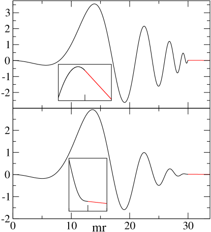
Figure 2: The rescaled coefficient $\Phi_{+}(t,r)$ for $\gamma=4,6$. Namely, $\Phi_{+}(t,r)\times 10^{4}m^{-3}$ at $mt=30$ for $\gamma=4$ (upper plot) and $\gamma=6$ (lower plot). Black (red) lines show data for $r<t$ ($r>t$). Insets magnify the area around $r=t$. Their width in the horizontal direction is $4\times 10^{-4}$ (upper plot) and $1$ (lower plot).

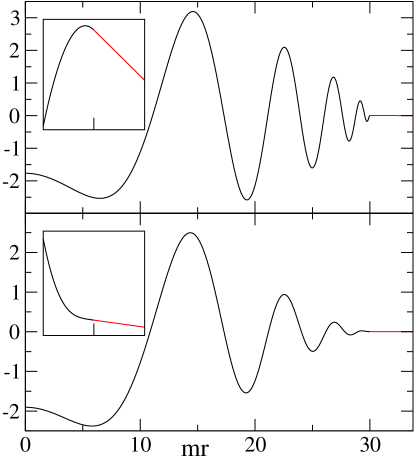
Figure 3: The same as in Fig. 2 except we show here $\Phi_{-}(t,r)$ instead of $\Phi_{+}(t,r)$. The horizontal width of the insets is $2\times 10^{-4}$ (upper plot) and $4\times 10^{-1}$ (lower plot).

First, the mean magnetic field for $\gamma=4,6,8\cdots$ and $r\geq t$, as well as $\gamma=2$ and $r>t$, can be analytically obtained by putting (15) into (41)

$$\langle\bm{B}(t,\bm{r})\rangle=\frac{3({\bm{\mu}}\cdot{\hat{\bm{r}}}){\hat{\bm{r}}}-{\bm{\mu}}}{4\pi r^{3}}\cos(mt)+\exp(-mr)\bm{b}(t,\bm{r}),$$ (42a)

$$\bm{b}(t,\bm{r})=\frac{{\bm{\mu}}}{4\pi r^{3}}\left(1+r\Delta_{r}+r^{2}\Delta_{r}^{2}\right)P_{\gamma}(mr,mt)\\ -\frac{3({\bm{\mu}}\cdot{\hat{\bm{r}}}){\hat{\bm{r}}}}{4\pi r^{3}}\left(1+r\Delta_{r}+\frac{r^{2}}{3}\Delta_{r}^{2}\right)P_{\gamma}(mr,mt),$$ (42b)

where $\Delta_{r}=m-\partial_{r}$. These expressions show that the dynamics of the mean magnetic field, in the $r>t$ region, is universal for $mt\gg 1$. Indeed, in such a case $\langle\bm{B}(t,\bm{r})\rangle$ practically does not depend on the parameter $\gamma$, which is not uniquely specified in our studies (29). The most important thing now is that for $r\to\infty$, we are left with the first term in (42a), which represents the magnetic field of the magnetic dipole having the periodically oscillating magnetic moment ${\bm{\mu}}\cos(mt)$.

Second, the dynamics of mean magnetic field (35) in the $r<t$ region is illustrated in Figs. 2 and 3, where we plot the coefficients $\Phi_{\pm}(t,r)$ for $\gamma=4,6$. In order to prepare these figures, we have numerically evaluated (37) and (38) via Mat , because we could not arrive at useful analytical expressions (in such a region of space) for $\gamma$’s greater than $2$ (the case of $\gamma=2$ is discussed in Secs. III.1–III.3). We see from Figs. 2 and 3 that the mean magnetic field oscillates in the $r<t$ region, where it reverses its direction. As we have numerically verified, the number (amplitude) of such oscillations increases (decreases) as a function of time. Note that such oscillations have a non-universal character because they depend on $\gamma$.

Third, the insets in Figs. 2 and 3 illustrate the continuity of the mean magnetic field across $r=t$ for $\gamma=4,6$ (such an observation also holds for larger $\gamma$’s). However, the mean magnetic field is weakly discontinuous at $r=t$ because there is a shock wave propagating in the studied system Rem (a). Indeed, the shock wave component of $\Phi_{\pm}(t,r)$ becomes evident after the computation of $\partial^{2}_{t}\Phi_{\pm}(t,r)$ for $\gamma=4$ and $\partial^{4}_{t}\Phi_{\pm}(t,r)$ for $\gamma=6$ (it can be shown with the help of BDP that such derivatives are discontinuous at $r=t$). We mention in passing that the numerical differentiation of the data from Figs. 2 and 3 supports the view that $\partial^{2}_{r}\Phi_{\pm}(t,r)$ for $\gamma=4$ and $\partial^{4}_{r}\Phi_{\pm}(t,r)$ for $\gamma=6$ are also discontinuous at $r=t$.

Fourth, under the mapping ${\bm{\mu}}\times{\hat{\bm{r}}}\to q{\hat{\bm{r}}}$, $\langle\bm{E}(t,\bm{r})\rangle$ given by (34) is equal to $\langle-m^{2}\bm{V}(t,\bm{r})\rangle$ computed in the states studied in BDP . Such a feature is rather unexpected given the fact that the states discussed in this work are of no interest in the context of the problem considered in BDP . Due to the above-mentioned mapping, we shall not discuss below the dynamics of the mean electric field in the magnetic dipole-charged states. We only mention that for $r>t$ and $\gamma$’s given by (29)

$$\langle\bm{E}(t,\bm{r})\rangle=m\frac{{\bm{\mu}}\times{\hat{\bm{r}}}}{4\pi r^{2}}\sin(mt)+O\left(\exp(-mr)\right).$$ (43)

Such a formula predicts $|\langle\bm{E}(t,\bm{r})\rangle|\sim\sin(\theta)r^{-2}$ for $r\to\infty$, where $\theta\in[0,\pi]$ is the angle between ${\bm{\mu}}$ and ${\hat{\bm{r}}}$. We find it interesting that despite the $r^{-2}$ asymptotic decay of $|\langle\bm{E}(t,\bm{r})\rangle|$,

$$\langle Q(t)\rangle=\lim_{r\to\infty}\int d\bm{S}(\bm{r})\cdot\langle\bm{E}(t,\bm{r})\rangle=0$$ (44)

in the discussed states ($d\bm{S}(\bm{r})$ is the surface element on the sphere of radius $r$). Physically, (44) follows from the fact that in the Proca theory one cannot construct the state in which $\langle Q(t)\rangle\neq 0$ without the longitudinal excitations (such excitations are absent in the studied magnetic dipole-charged states) Rem (e). Technically, (44) can be explained by the fact that $\langle\bm{E}(t,\bm{r})\rangle$ is perpendicular to $d\bm{S}(\bm{r})$, which is so not only asymptotically (43) but also for any $r>0$ (34). Finally, we note that we find the axisymmetric topology of (34) rather surprising for the following reasons (Fig. 4). On the one hand, it is so much different from the topology of the Coulomb field despite the fact that such a field is also falling off as $r^{-2}$. On the other hand, it is the same as the topology of the velocity field of points on a rotating sphere despite the fact that such a system bears no obvious similarity to the one discussed in this work.

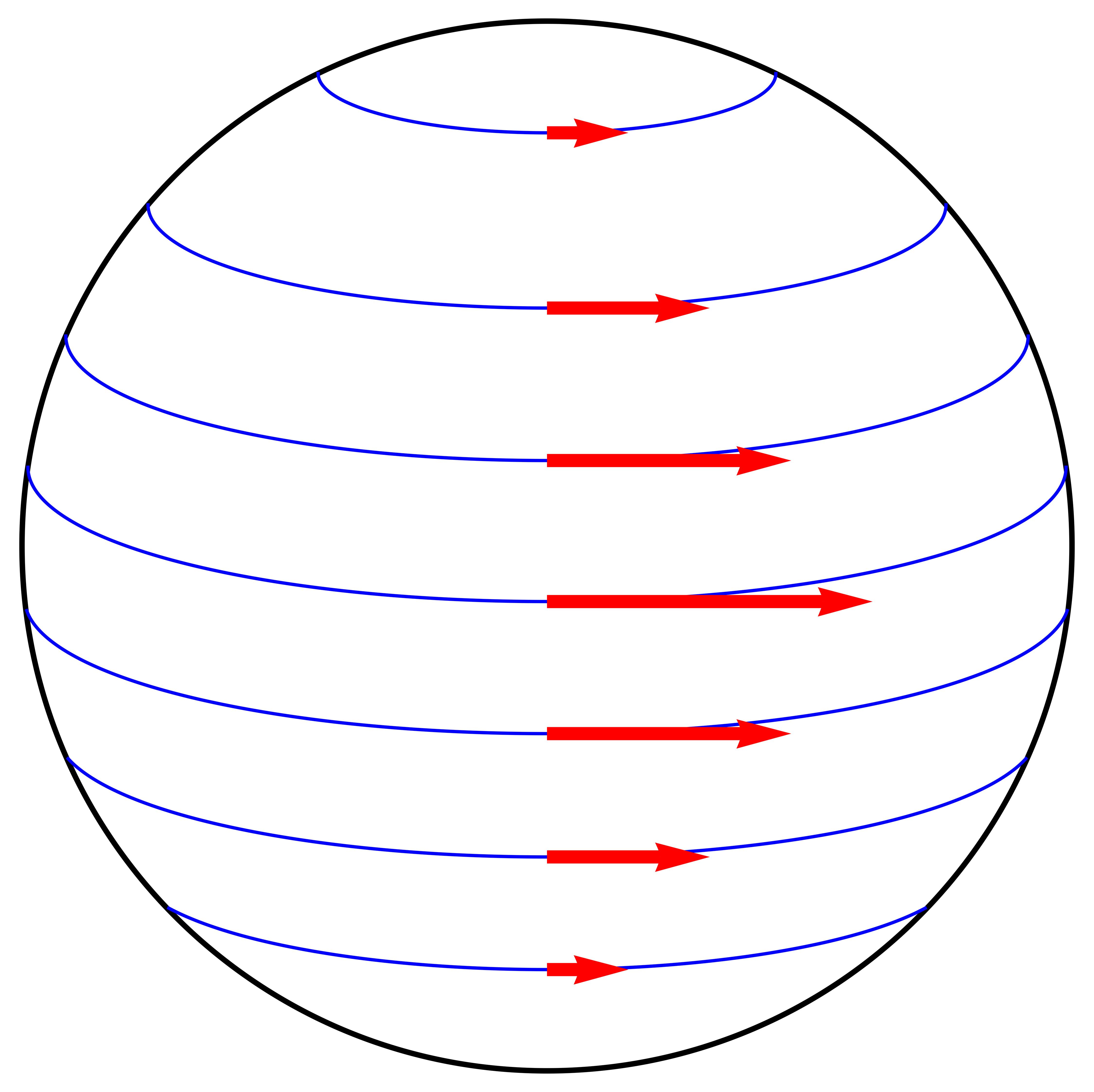
Figure 4: Schematic plot of mean electric field (34) on the sphere of radius $r$. The magnetic moment ${\bm{\mu}}$ is oriented vertically (it points upwards). The mean electric field $\langle\bm{E}(t,\bm{r})\rangle$ is presented with red arrows at a given set of points ($\Phi(t,r)>0$ is assumed). It is symmetric with respect to rotations around the axis that is parallel to ${\bm{\mu}}$ and goes through the center of the sphere. The field lines are depicted in blue, they are tangent to $\langle\bm{E}(t,\bm{r})\rangle$.

Fifth, we note that the mean electric and magnetic fields are perpendicular to each other, which is seen from (34) and (35). Somewhat more interestingly, we observe that the asymptotic algebraic decay of the mean electric field is slower than the one of the mean magnetic field, which is seen from (42b) and (43).

Till the end of this section, we will discuss the $\gamma=2$ case, where one can obtain additional analytical insights into the non-equilibrium dynamics of the mean electromagnetic field in magnetic dipole-charged states.

III.1 $\gamma=2$: shock wave discontinuity

The key difference between the $\gamma=2$ case and $\gamma=4,6,8,\cdots$ cases is that the mean magnetic field is discontinuous (continuous) at $r=t$ in the former (latter) case(s). Such a discontinuity, which is illustrated in the insets of Figs. 5 and 6, can be explained as follows.

We gather from the results presented in BDP that

$$\partial_{r}\phi_{2}(t,r)=\partial_{r}\int_{0}^{\infty}d\omega_{k}\cdots=\int_{0}^{\infty}d\omega_{k}\partial_{r}(\cdots)$$ (45)

for any $r,t>0$, whereas

$$\partial^{2}_{r}\phi_{2}(t,r)=\partial^{2}_{r}\int_{0}^{\infty}d\omega_{k}\cdots=\int_{0}^{\infty}d\omega_{k}\partial^{2}_{r}(\cdots)$$ (46)

for any $r,t>0$ as long as $r\neq t$. These expressions imply that for $r\neq t$, the mean magnetic field can be computed from (35) combined with (41); see the comments below (41). Thereby, to get insights into $\langle\bm{B}(t,\bm{r})\rangle$ near $r=t$, we take a close look at $\partial_{r}\phi_{2}$ and $\partial^{2}_{r}\phi_{2}$. Following BDP , we observe that

$$\lim_{r\to t^{-}}\partial_{r}\phi_{2}(t,r)=\lim_{r\to t^{+}}\partial_{r}\phi_{2}(t,r),$$ (47)

whereas

$$\lim_{r\to t^{-}}\partial^{2}_{r}\phi_{2}(t,r)=\frac{m^{2}}{4\pi t}+\lim_{r\to t^{+}}\partial^{2}_{r}\phi_{2}(t,r).$$ (48)

This implies that $\Phi_{\pm}(t,r)$ for $\gamma=2$ are discontinuous at $r=t$ and so is mean magnetic field (35)

$$\lim_{r\to t^{+}}\langle\bm{B}(t,r{\hat{\bm{r}}})\rangle-\lim_{r\to t^{-}}\langle\bm{B}(t,r{\hat{\bm{r}}})\rangle=-\frac{m^{2}}{4\pi t}({\bm{\mu}}\cdot{\hat{\bm{r}}}){\hat{\bm{r}}}+\frac{m^{2}}{4\pi t}{\bm{\mu}}.$$ (49)

In other words, there is a shock wave discontinuity propagating with the speed of light in the discussed quantity.

The question now is what can be said about the value of the mean magnetic field at the shock wave front. It turns out that there is a curious ambiguity concerning this issue. Namely,

$$\langle\bm{B}(t,t{\hat{\bm{r}}})\rangle =\left.\langle{\bm{\nabla}}\times\bm{V}(t,\bm{r})\rangle\right|_{r=t}$$ (50a)

$$\neq\left.{\bm{\nabla}}\times\langle\bm{V}(t,\bm{r})\rangle\right|_{r=t},$$ (50b)

which triggers the following remarks.

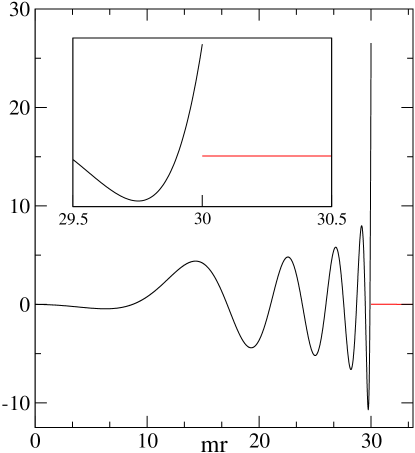
Figure 5: The rescaled coefficient $\Phi_{+}(t,r)$ for $\gamma=2$. Namely, $\Phi_{+}(t,r)\times 10^{4}m^{-3}$ at $mt=30$. The black line comes from (56), whereas the red one from (54). The inset magnifies the area around the shock wave discontinuity.

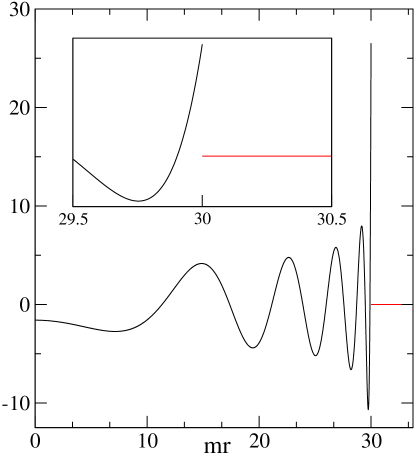
Figure 6: The same as in Fig. 5 except we show here $\Phi_{-}(t,r)$ instead of $\Phi_{+}(t,r)$.

First, (50a) is given by (35) with $\Phi_{\pm}(t,r=t)$ obtained from (37) and (38). For $\gamma=2$, the integrals in (37) and (38) can be calculated with the help of the results presented in BDP . Indeed, by expressing the spherical Bessel functions in terms of trigonometric functions, we have found that (37) and (38) are given by linear combinations of three integrals that were computed in BDP . By following such a procedure, we have found that $\Phi_{\pm}(t,r=t)$ is given by

$$\beta_{\pm}\frac{\cos(mt)-(1+mt)\exp(-mt)}{4\pi t^{3}}+m^{2}\frac{1/2-\exp(-mt)}{4\pi t},$$ (51)

where $\beta_{\pm}=2\pm 1$. This result turns out to be half-way between the discontinuities on both sides of the shock wave front. Namely, (51) is equal to

$$\frac{1}{2}\lim_{r\to t^{-}}\Phi_{\pm}(t,r)+\frac{1}{2}\lim_{r\to t^{+}}\Phi_{\pm}(t,r),$$ (52)

which is seen from (54) and (59).

Second, by computing the curl of

$$\langle\bm{V}(t,\bm{r})\rangle=-\partial_{r}\phi_{2}(t,r){\bm{\mu}}\times{\hat{\bm{r}}},$$ (53)

one may verify that (50b) is given by (35) with $\Phi_{\pm}(t,r=t)$ obtained from (41). Such an expression is undefined because $\partial_{r}^{2}\phi_{2}(t,r=t)$ does not exist BDP . We mention in passing that (53) can be established for all $r,t>0$ with the help of (6e), (13), (26), and (45).

Third, we expect that (50a) answers the question of what is the mean magnetic field at the shock wave front. However, we lack a definite argument explaining why such a quantity should not be approached via (50b). Thereby, we leave open the issue discussed here.

Finally, we mention that similar observations apply to mean electric field (34) for $\gamma=2$. Such a quantity is also discontinuous at $r=t$, which can be linked to the fact that $\partial_{t}\partial_{r}\phi_{2}(t,r)$ is discontinuous there BDP . Moreover, there is an ambiguity in the evaluation of such a mean electric field at the shock wave front. Namely, $\langle\bm{E}(t,t{\hat{\bm{r}}})\rangle=\left.\langle-\partial_{t}\bm{V}(t,\bm{r})\rangle\right|_{r=t}$, which is given by (34) combined with (36), is not equal to $-\left.\partial_{t}\langle\bm{V}(t,\bm{r})\rangle\right|_{r=t}$ that is given by (34) combined with (40). The former quantity is finite and it can be extracted out of BDP via the mapping stated above (44), whereas the latter one is undefined because $\partial_{t}\partial_{r}\phi_{2}(t,r=t)$ does not exist BDP .

III.2 $\gamma=2$: $r>t$ region

In the $r>t$ region, we find for $\gamma=2$ that

$$\Phi_{\pm}(t,r)=\beta_{\pm}\frac{\cos(mt)-(1+mr)\exp(-mr)}{4\pi r^{3}}\\ -\frac{m^{2}}{4\pi r}\exp(-mr).$$ (54)

Such a result is obtained by putting (15) into (41) and noting that $P_{2}(a,b)=1$. It determines the mean magnetic field, in the considered region of space, via (35).

III.3 $\gamma=2$: $r<t$ region

To begin, we note that we know from BDP that for $0<r<t$

$$\phi_{2}(t,r)=\frac{\cos(mr)-\exp(-mr)}{4\pi r}\\ -\frac{1}{4\pi r}\int_{mr}^{mt}dy\int_{0}^{mr}dx{\rm J}_{0}\left(\sqrt{y^{2}-x^{2}}\right),$$ (55)

where ${\rm J}_{n}$ is the Bessel function of the first kind of order $n$. This can be used to show that for such $r,t$ and $\gamma=2$, the coefficients from (35) satisfy

$$4\pi r^{3}\Phi_{\pm}(t,r) =\beta_{\pm}4\pi r\phi_{2}(t,r)-\beta_{\pm}mr\exp(-mr)$$

$$+\beta_{\pm}mr\int_{mr}^{mt}dx{\rm J}_{0}\left(\sqrt{x^{2}-(mr)^{2}}\right)$$

$$+(mr)^{2}[1-\exp(-mr)]$$

$$-(mr)^{3}\int_{mr}^{mt}dx\frac{{\rm J}_{1}\left(\sqrt{x^{2}-(mr)^{2}}\right)}{\sqrt{x^{2}-(mr)^{2}}}.$$ (56)

We have obtained this fairly complicated result via standard formulas associated with Bessel functions: ${\textstyle\int}_{0}^{x}dy{{\rm J}_{0}}\left(\sqrt{x^{2}-y^{2}}\right)=\sin(x)$ coming from formula 6.517 of Gradshteyn et al. (2014), $d{{\rm J}_{0}}(x)/dx=-{{\rm J}_{1}}(x)$, etc. We have simplified it near $r=0$ and $r=t^{-}$.

Near $r=0$, (56) can be reduced to

$$\Phi_{\pm}(t,r)=\frac{m^{3}}{12\pi}(1\mp 1)F(mt)+O(r^{2}),$$ (57a)

$$F(x)=1+{\rm J}_{1}(x)\\ -x{\rm J}_{0}(x)-\frac{\pi x}{2}{\rm J}_{1}(x){\rm H}_{0}(x)+\frac{\pi x}{2}{\rm J}_{0}(x){\rm H}_{1}(x),$$ (57b)

where ${\rm H}_{n}$ represents the Struve function of order $n$ (similar expressions appear in BDP , where the function $F(x)$ is introduced and briefly discussed in a different context). We see from (57b) that $\Phi_{+}(t,r=0)$ vanishes. Somewhat more interestingly, (57b) can be used to show that $\Phi_{-}(t,r=0)$ exhibits damped oscillations, which are accurately described for $mt\gg 1$ by the formula

$$\frac{2}{3}\left(\frac{m}{2\pi t}\right)^{3/2}\sin\left(mt+\frac{\pi}{4}\right).$$ (58)

Near $r=t^{-}$, (56) leads to

$$\lim_{r\to t^{-}}\Phi_{\pm}(t,r)=\beta_{\pm}\frac{\cos(mt)-(1+mt)\exp(-mt)}{4\pi t^{3}}\\ +m^{2}\frac{1-\exp(-mt)}{4\pi t}.$$ (59)

Such a result shows that $\Phi_{\pm}(t,r=t^{-})$ decays as $1/t$ for $mt\gg 1$. This can be compared to the decay of $\Phi_{\pm}(t,r=t^{+})$, which according to (54) proceeds as $1/t^{3}$ for $mt\gg 1$. Thereby, the mean magnetic field near $r=t$ is dominated for $mt\gg 1$ by the contribution from the region of space, which has just been swept by the shock wave front. The insets in Figs. 5 and 6 illustrate this observation.

The dynamics of $\Phi_{\pm}(t,r)$ for $\gamma=2$ and $r<t$ is depicted in Figs. 5 and 6. To prepare them, we have numerically evaluated the integrals from (56) via Mat . Apart from the shock wave discontinuity, these figures are qualitatively similar to Figs. 2 and 3, which we have just discussed. Therefore, we shall not dwell on them.

IV Electric dipole-charged states

The states of interest here will be constructed so as to yield $\langle\bm{B}(0,\bm{r})\rangle=\bm{0}$ for $r\geq 0$ and

$$\langle\bm{E}(0,\bm{r})\rangle=\frac{3(\bm{d}\cdot{\hat{\bm{r}}}){\hat{\bm{r}}}-\bm{d}}{4\pi r^{3}}$$ (60)

for $r\to\infty$, where $\bm{d}$ is the electric dipole moment.

To achieve this goal, we consider the ansatz

$$\chi(\bm{x})=\int\frac{d^{3}\mkern-1.5muk\,}{(2\pi)^{3/2}}g({\bm{k}})a_{{\bm{k}}3}\exp(\mathrm{i}{\bm{k}}\cdot\bm{x})+\text{h.c.},$$ (61)

where $g({\bm{k}})\in\mathbbm{R}$, which via (7), (8), and (13) leads to $\langle\bm{B}(0,\bm{r})\rangle=\bm{0}$ and

$$\langle\bm{E}(0,\bm{r})\rangle=\frac{1}{2}\int\frac{d^{3}\mkern-1.5muk\,}{(2\pi)^{3}}\sqrt{\frac{2}{\varepsilon_{k}}}\frac{m}{\omega_{k}}g({\bm{k}}){\bm{k}}\exp(\mathrm{i}{\bm{k}}\cdot\bm{r})+\text{c.c.}$$ (62)

If we substitute

$$g({\bm{k}})=-\sqrt{\frac{\varepsilon_{k}}{2m^{2}}}\frac{\bm{d}\cdot{\bm{k}}}{\omega_{k}}$$ (63)

into (62), replace $(\bm{d}\cdot{\bm{k}}){\bm{k}}$ by $-(\bm{d}\cdot{\bm{\nabla}}){\bm{\nabla}}$, and uncritically reverse the order of differentiation and integration, we find that the resulting expression is the same as (60) for all $r>0$. Such a procedure of the evaluation of $\langle\bm{E}(0,\bm{r})\rangle$, however, is unjustified. In fact, as can be easily verified with the help of (25), the situation here is analogous to the one discussed in Sec. III. Thereby, it should come as no surprise that we again introduce the bounded function $f(\omega_{k})\in\mathbbm{R}$ and proceed via

$$\chi(\bm{x})\to\chi(\bm{x})=\\ -\int\frac{d^{3}\mkern-1.5muk\,}{(2\pi)^{3/2}}\sqrt{\frac{\varepsilon_{k}}{2m^{2}}}\frac{\bm{d}\cdot{\bm{k}}}{\omega_{k}}f(\omega_{k})a_{{\bm{k}}3}\exp(\mathrm{i}{\bm{k}}\cdot\bm{x})+\text{h.c.},$$ (64)

where $f(\omega_{k})$ vanishing faster than $1/\omega_{k}$ for $\omega_{k}\to\infty$ ensures the UV convergence of the integral determining $\langle\bm{E}(0,\bm{r})\rangle$, whereas $f(\omega_{k}\to 0)\to 1$ protects the proper asymptotic form of such a mean electric field.

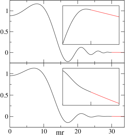
Figure 7: The rescaled coefficient $\frac{1}{2}[\Phi_{+}(t,r)-\Phi_{-}(t,r)]$ for $\gamma=4,6$. Namely, $\frac{1}{2}[\Phi_{+}(t,r)-\Phi_{-}(t,r)]\times 10^{4}m^{-3}$ at $mt=30$ for $\gamma=4$ (upper plot) and $\gamma=6$ (lower plot). Black (red) lines show data for $r<t$ ($r>t$). Insets magnify the area around $r=t$. Their width in the horizontal direction is $4\times 10^{-1}$ (upper plot) and $2$ (lower plot).

Further constraints on $f$ come from (10) and (11) leading to

$$1=\alpha^{2}+\frac{d^{2}}{12\alpha^{2}\pi^{2}m^{2}}\int_{0}^{\infty}d\omega_{k}\omega_{k}^{2}\varepsilon_{k}f^{2}(\omega_{k}),\ d=|\bm{d}|$$ (65)

and

$${\cal H}=\frac{d^{2}}{12\alpha^{2}\pi^{2}m^{2}}\int_{0}^{\infty}d\omega_{k}\omega_{k}^{2}\varepsilon_{k}^{2}f^{2}(\omega_{k}),$$ (66)

which substantially differ from (27) and (28), respectively. In fact, $f(\omega_{k})$ vanishing faster than $1/\omega_{k}^{5/2}$ for $\omega_{k}\to\infty$ has to be assumed now. We again choose $f(\omega_{k})$ given by (30). This time, however, we consider

$$\gamma=4,6,8,\cdots.$$ (67)

The evaluation of (65) and (66) via (31) leads to

$$\alpha^{2}=\frac{1}{2}\left(1\pm\sqrt{1-\left(\frac{d}{d_{\text{max}}}\right)^{2}}\right),$$ (68a)

$$d_{\text{max}}=\sqrt{\frac{12\pi^{3/2}\Gamma(\gamma-1/2)}{m^{2}\Gamma(\gamma-2)}},$$ (68b)

$${\cal H}=m\frac{(md)^{2}\Gamma(\gamma-5/2)}{48\alpha^{2}\pi^{3/2}\Gamma(\gamma-1)},$$ (69)

where $d_{\text{max}}$ provides the upper bound on the magnitude of the electric dipole moment that can be encoded in the states studied in this section.

The field configuration, in the discussed electric-dipole charged states, is characterized by

$$\langle\bm{E}(t,\bm{r})\rangle=\Phi_{+}(t,r)(\bm{d}\cdot{\hat{\bm{r}}}){\hat{\bm{r}}}-\frac{\Phi_{+}(t,r)-\Phi_{-}(t,r)}{2}\bm{d},$$ (70)

$$\langle\bm{B}(t,\bm{r})\rangle=\bm{0},$$ (71)

where $\Phi_{\pm}(t,r)$ are given by (37) and (38). Several remarks are in order now.

First, we note that for $\gamma$’s being of interest here (67), one may equivalently evaluate (70) via (41) for all ${r,t>0}$. We also note that mean electric field (70) is weakly discontinuous at $r=t$ for such $\gamma$’s Rem (a).

Second, by combining (70) with (41) and (15), we have found that for $r\geq t$ and $\gamma$ given by (67)

$$\langle\bm{E}(t,\bm{r})\rangle=\frac{3(\bm{d}\cdot{\hat{\bm{r}}}){\hat{\bm{r}}}-\bm{d}}{4\pi r^{3}}\cos(mt)+\exp(-mr)\bm{e}(t,\bm{r}),$$ (72a)

$$\bm{e}(t,\bm{r})=\frac{\bm{d}}{4\pi r^{3}}(1+r\Delta_{r})P_{\gamma}(mr,mt)\\ -\frac{3(\bm{d}\cdot{\hat{\bm{r}}}){\hat{\bm{r}}}}{4\pi r^{3}}\left(1+r\Delta_{r}+\frac{r^{2}}{3}\Delta_{r}^{2}\right)P_{\gamma}(mr,mt).$$ (72b)

The hallmark feature of such a solution is that in the limit of large $r$, we are left in (72a) with the field of the electric dipole having the periodically oscillating dipole moment $\bm{d}\cos(mt)$.

Third, the dynamics of the coefficient in the first term in (70) is depicted in Fig. 2 for $\gamma$’s that are of interest here. The dynamics of the coefficient in the second term in (70) is illustrated in Fig. 7, which is directly related to Figs. 2 and 3. Thereby, we shall not dwell on it.

Fourth, mean electromagnetic field (70) and (71) is interesting from the Maxwell theory perspective. Namely, due to the identity Rem (f)

$${\bm{\nabla}}\times\langle\bm{E}\rangle=-\partial_{t}\langle\bm{B}\rangle,$$ (73)

which holds not only in the Maxwell theory but also in the Proca theory, one may guess that (70) can be written as the gradient of a scalar because the right-hand side of (73) vanishes due to (71). This is indeed the case as it turns out that (70) can be also expressed as

$$\langle\bm{E}(t,\bm{r})\rangle={\bm{\nabla}}[\bm{d}\cdot{\bm{\nabla}}\phi_{\gamma}(t,r)].$$ (74)

Then, we note that the time-dependence of the mean electric field, in the presence of the vanishing mean magnetic field, suggests the existence of the mean current in our system. Such a suggestion, based on the intuition coming from the Maxwell theory, appears to be confusing at first sight because there is no external current in our calculations. However, it turns out to be correct because in the Proca theory Rem (f)

$${\bm{\nabla}}\times\langle\bm{B}\rangle=\langle\bm{J}\rangle+\partial_{t}\langle\bm{E}\rangle,$$ (75)

where $\bm{J}=-m^{2}\bm{V}$ is the internal $3$-current operator of theory (1) (see BDP for its recent discussion in the context relevant for these studies). We mention in passing that the internal Proca current, in the classical Proca theory, is commented upon in Goldhaber and Nieto (2010).

V Summary

We have discussed the dynamics of field configurations encoded in the particular class of electric and magnetic dipole-charged states in the Proca theory. The key universal features of our results can be transparently presented by taking a look at the asymptotic fields

$$\langle\bm{E}(t,\bm{r})\rangle_{\infty}=\langle\bm{E}(t,\bm{r})\rangle\ \text{for}\ r\to\infty,$$ (76)

$$\langle\bm{B}(t,\bm{r})\rangle_{\infty}=\langle\bm{B}(t,\bm{r})\rangle\ \text{for}\ r\to\infty,$$ (77)

which are obtained by discarding the short-distance terms in (42b), (43), and (72b). In our magnetic dipole-charged states

$$\langle\bm{B}(t,\bm{r})\rangle_{\infty}=\frac{3({\bm{\mu}}\cdot{\hat{\bm{r}}}){\hat{\bm{r}}}-{\bm{\mu}}}{4\pi r^{3}}\cos(mt),$$ (78)

$$\langle\bm{E}(t,\bm{r})\rangle_{\infty}=m\frac{{\bm{\mu}}\times{\hat{\bm{r}}}}{4\pi r^{2}}\sin(mt),$$ (79)

whereas in our electric dipole-charged states

$$\langle\bm{E}(t,\bm{r})\rangle_{\infty}=\frac{3(\bm{d}\cdot{\hat{\bm{r}}}){\hat{\bm{r}}}-\bm{d}}{4\pi r^{3}}\cos(mt),$$ (80)

$$\langle\bm{B}(t,\bm{r})\rangle_{\infty}=\bm{0}.$$ (81)

The first thing we learn from these results is that the asymptotic fields satisfy the harmonic oscillator equation

$$\partial^{2}_{t}\langle O(t,\bm{r})\rangle_{\infty}=-m^{2}\langle O(t,\bm{r})\rangle_{\infty},$$ (82)

where $O=\bm{E},\bm{B}$. The second one is that according to (78) [(80)], the studied magnetic [electric] dipole-charged field configurations are characterized by the periodically oscillating magnetic [electric] dipole moment ${\bm{\mu}}\cos(mt)$ [$\bm{d}\cos(mt)$]. Therefore, our results provide the concrete theoretical illustration of the phenomenon of the periodic oscillations of the dipole moments in the Proca theory, which to the best of our knowledge has not been discussed in the literature before.

We have also discussed the non-equilibrium dynamics of our electric and magnetic dipole-charged field configurations at intermediate distances, where the shock wave phenomenon seems to be most interesting. Namely, our solutions are either discontinuous or weakly discontinuous and these discontinuities are propagating. We find it interesting that such singularities appear despite the fact that the studied quantum states are well-defined. Indeed, they are normalizable and represent finite-energy field configurations.

The non-equilibrium character of our solutions stems from the fact that there is no external current keeping the fields in place. As a result of that, the fields escape from their initial arrangement. Thereby, we say that we deal with escaping (outgoing) solutions in this work. One can also analyze collapsing (incoming) solutions by the continuation of our results from the time domain $[0,\infty)$ to $(-\infty,0)$.

The physical realization of the discussed states is problematic because (i) it is unclear what stable particle could be described by the Proca theory and (ii) causality considerations prohibit the laboratory-based creation of the dipole-charged states. Regarding the (i) issue, we mention that it is still possible that the photon is a massive particle Tu et al. (2005); Goldhaber and Nieto (2010); other options may arise in the future. Regarding the (ii) issue, we mention that the scenario, where the evolution starts at $t=-\infty$ and the fields undergo initially collapsing dynamics, somewhat avoids the problem with the experimental creation of the dipole-charged states.

Finally, we would like to say that our studies give definite insights into the structure and dynamics of the IR sector of the Proca theory. This is a fairly unexplored topic because short range fields are traditionally associated with such a theory. We would like to stress that the characterization of the IR sector of the Proca theory poses a well-defined mathematical problem and it contributes to the in-depth understanding of such a paradigmatic theory of a massive vector field.

APPENDIX A CONVENTIONS

We adopt the Heaviside-Lorentz system of units in its $\hbar=c=1$ version. Greek and Latin indices of tensors take values $0,1,2,3$ and $1,2,3$, respectively. The metric signature is $(+---)$. $3$-vectors are written in bold, e.g. $x=(x^{\mu})=(x^{0},\bm{x})$. We use the Einstein summation convention, $(X_{\mu\cdots})^{2}=X_{\mu\cdots}X^{\mu\cdots}$. $\partial_{X}=\partial/\partial X$ and $X^{+}$ ($X^{-}$) denotes the quantity that is infinitesimally larger (smaller) than $X$. The hermitian (complex) conjugation is denoted as h.c. (c.c.).

APPENDIX B $P_{\gamma}$ polynomials

The following formula for the $P_{\gamma}$ polynomials, which we have introduced in this work in (15), was given in BDP

$$P_{\gamma}(a,b)=-\exp(a)\text{Res}(f(z),\mathrm{i}\pi/2),$$ (83a)

$$f(z)=\frac{\cos[b\operatorname{ch}(z)]\exp[\mathrm{i}a\operatorname{sh}(z)]}{\operatorname{sh}(z)\operatorname{ch}^{\gamma-1}(z)},$$ (83b)

where $\gamma=2,4,6,\cdots$ and ${\rm Res}(f(z),z_{0})$ stands for the residue of the function $f(z)$ at $z_{0}$. Given the fact that $f(z)$ has the pole of order $\gamma-1$ at $z=\mathrm{i}\pi/2$, the above expression is fairly complicated. We will derive another formula below, the one allowing for the recursive evaluation of $P_{\gamma}(a,b)$.

To begin, we introduce dimensionless variables

$$a=mr,\ b=mt$$ (84)

and the following function

$$\widehat{\phi}_{\gamma}(a,b)=4\pi r\phi_{\gamma}(t,r)\\ =\frac{2}{\pi}\int_{0}^{\infty}d\omega\frac{\cos\left(b\sqrt{1+\omega^{2}}\right)}{(1+\omega^{2})^{\gamma/2}}\frac{\sin(a\omega)}{\omega},$$ (85)

which for $a\geq b\geq 0$ reduces to BDP

$$\widehat{\phi}_{\gamma}(a,b)=\cos(b)-P_{\gamma}(a,b)\exp(-a).$$ (86)

Note that unlike $\widehat{\phi}_{\gamma}(a,b)$, the $P_{\gamma}(a,b)$ polynomials are insensitive to the relation between $a$ and $b$, which is seen from (83).

For

$$\gamma=4,6,8,\cdots$$ (87)

being of interest from now on, we find that

$$\partial_{b}^{2}\widehat{\phi}_{\gamma}(a,b)=-\widehat{\phi}_{\gamma-2}(a,b).$$ (88)

Such an equation follows from the fact that according to BDP , $\partial_{b}^{2}$ can be taken under the integral symbol in (85) during the evaluation of the left-hand side of (88).

By combining (86) with (88), we arrive at

$$\partial_{b}^{2}P_{\gamma}(a,b)=-P_{\gamma-2}(a,b),$$ (89)

whose solution can be written as

$$P_{\gamma}(a,b)=P_{\gamma}(a,0)-\int_{0}^{b}dy\int_{0}^{y}dxP_{\gamma-2}(a,x).$$ (90)

Note that the double integration of (89) over $b$ does not lead to the term linear in $b$ because $P_{\gamma}(a,b)$ is even in $b$, which follows from (83).

The expression for $P_{\gamma}(a,0)$ can be directly obtained from the $b=0$ version of (85). Namely, formula 3.737.3 of Gradshteyn et al. (2014) yields

$$P_{\gamma}(a,0)=P_{\gamma-2}(a,0)+\frac{a}{\gamma-2}\left(1-\frac{d}{da}\right)P_{\gamma-2}(a,0).$$ (91)

By combining (90) with (91), (16) is established.