Revisiting the computation of the critical points of the Keplerian distance

Abstract

We consider the Keplerian distance $d$ in the case of two elliptic orbits, i.e. the distance between one point on the first ellipse and one point on the second one, assuming they have a common focus. The absolute minimum $d_{\rm min}$ of this function, called MOID or orbit distance in the literature, is relevant to detect possible impacts between two objects following approximately these elliptic trajectories. We revisit and compare two different approaches to compute the critical points of $d^{2}$, where we squared the distance $d$ to include crossing points among the critical ones. One approach uses trigonometric polynomials, the other uses ordinary polynomials. A new way to test the reliability of the computation of $d_{\rm min}$ is introduced, based on optimal estimates that can be found in the literature. The planar case is also discussed: in this case we present an estimate for the maximal number of critical points of $d^{2}$, together with a conjecture supported by numerical tests.

1 Introduction

The distance $d$ between two points on two Keplerian orbits with a common focus, that we call Keplerian distance, appears in a natural way in Celestial Mechanics. The absolute minimum of $d$ is called MOID (minimum orbital intersection distance), or simply orbit distance in the literature, and we denote it by $d_{\rm min}$. It is important to be able to track $d_{\rm min}$, and actually all the local minimum points of $d$, to detect possible impacts between two celestial bodies following approximately these trajectories, e.g. an asteroid with the Earth [16, 17], or two Earth satellites [19]. Moreover, the information given by $d_{\rm min}$ is useful to understand observational biases in the distribution of the known population of NEAs, see [13]. Because of the growing number of Earth satellites (e.g. the mega constellations of satellites that are going to be launched [2]) and discovered asteroids, fast and reliable methods to compute the minimum values of $d$ are required.

The computation of the minimum points of $d$ can be performed by searching for all the critical points of $d^{2}$, where considering the squared distance allows us to include trajectory-crossing points in the results.

There are several papers in the literature concerning the computation of the critical points of $d^{2}$, e.g. [20, 7, 15, 9, 10, 3].

Some authors also propose methods for a fast computation of $d_{\rm min}$ only, e.g. [21, 14].

We will focus on an algebraic approach for the case of two elliptic trajectories, as in [15], [9]. In [15] the critical points of $d^{2}$ are found by computing the roots of a trigonometric polynomial $g(u)$ of degree 8, where $u$ is the eccentric anomaly parametrizing one of the trajectories. The polynomial $g(u)$ is obtained by the computation of a Groebner basis, implying that generically we can not solve this problem by a polynomial with a smaller degree. In [9], resultant theory is applied to a system of two bivariate ordinary polynomials, together with the discrete Fourier transform, to obtain (generically) a univariate polynomial of degree 20 in a variable $t$, with a factor $(1+t^{2})^{2}$ leading to 4 pure imaginary roots that are discarded, so that we may have at most 16 real roots. Note that the trigonometric polynomial $g(u)$ of degree 8 corresponds to an ordinary polynomial of degree 16 in the variable $t$ through the transformation $t=\tan(u/2)$. These methods were extended to the case of unbounded conics with a common focus in [3], [10].

In this paper we revisit the computation of the critical points of $d^{2}$ for two elliptic trajectories by applying resultant theory to polynomial systems written in terms of the eccentric or the true anomalies. We obtain different methods using either ordinary or trigonometric polynomials. Moreover, we are able to compute via resultant theory the 8-th degree trigonometric polynomial $g(u)$ found by [15], and its analogue using the true anomalies (see Sections 4, 5). Some numerical tests comparing these methods are presented. We also test the reliability of the methods by taking advantage of the estimates for the values of $d_{\rm min}$ introduced in [13] when one trajectory is circular. For the case of two ellipses, since we do not have such estimates for $d_{\rm min}$, we use the optimal bounds for the nodal distance $\delta_{\rm nod}$ derived in [11].

After introducing some notation in Section 2, we deal with the problem using eccentric anomalies and ordinary polynomials in Section 3. In Sections 4 and 5 we describe other procedures employing trigonometric polynomials and, respectively, eccentric or true anomalies. Some numerical tests and the reliability of our computations are discussed in Section 6. Finally, we present results for the maximum number of critical points in the planar problem in Section 7, and draw some conclusions in Section 8. Additional details of the computations can be found in the Appendix.

2 Preliminaries

Let ${\cal E}_{1}$ and ${\cal E}_{2}$ be two confocal elliptic trajectories, with ${\cal E}_{i}$ defined by the five Keplerian orbital elements $a_{i},e_{i},i_{i},\Omega_{i},\omega_{i}$. We introduce the Keplerian distance

$$d(V)=\sqrt{\langle{\cal X}_{1}-{\cal X}_{2},{\cal X}_{1}-{\cal X}_{2}\rangle},$$ (1)

where ${\cal X}_{1},{\cal X}_{2}\in\mathbb{R}^{3}$ are the Cartesian coordinates of a point on ${\cal E}_{1}$ and a point on ${\cal E}_{2}$, corresponding to the vector $V=(v_{1},v_{2})$, where $v_{i}$ is a parameter along the trajectory ${\cal E}_{i}$. In this paper we will parametrize the orbits either with the eccentric anomalies $u_{i}$ or with the true anomalies $f_{i}$.

Let $(x_{1},y_{1})$ and $(x_{2},y_{2})$ be Cartesian coordinates of two points on the two trajectories, each in its respective plane. The origin for both coordinate systems is the common focus of the two ellipses. We can write

$${\mathcal{X}}_{1} =x_{1}\,{\mathcal{P}}+y_{1}\,{\mathcal{Q}},$$

$${\mathcal{X}}_{2} =x_{2}\,{\mathfrak{p}}+y_{2}\,{\mathfrak{q}},$$

with

$${\mathcal{P}} =\left(P_{x}\,,P_{y}\,,P_{z}\right), {\mathcal{Q}} =\left(Q_{x}\,,Q_{y}\,,Q_{z}\right),$$

$${\mathfrak{p}} =\left(p_{x}\,,p_{y}\,,p_{z}\right), {\mathfrak{q}} =\left(q_{x}\,,q_{y}\,,q_{z}\right),$$

where

$$P_{x}=\cos\omega_{1}\cos\Omega_{1}-\cos i_{1}\sin\omega_{1}\sin\Omega_{1},$$

$$P_{y}=\cos\omega_{1}\sin\Omega_{1}+\cos i_{1}\sin\omega_{1}\cos\Omega_{1},$$

$$P_{z}=\sin\omega_{1}\sin i_{1},$$

$$Q_{x}=-\sin\omega_{1}\cos\Omega_{1}-\cos i_{1}\cos\omega_{1}\sin\Omega_{1},$$

$$Q_{y}=-\sin\omega_{1}\sin\Omega_{1}+\cos i_{1}\cos\omega_{1}\cos\Omega_{1},$$

$$Q_{z}=\cos\omega_{1}\sin i_{1},$$

$$p_{x}=\cos\omega_{2}\cos\Omega_{2}-\cos i_{2}\sin\omega_{2}\sin\Omega_{2},$$

$$p_{y}=\cos\omega_{2}\sin\Omega_{2}+\cos i_{2}\sin\omega_{2}\cos\Omega_{2},$$

$$p_{z}=\sin\omega_{2}\sin i_{2},$$

$$q_{x}=-\sin\omega_{2}\cos\Omega_{2}-\cos i_{2}\cos\omega_{2}\sin\Omega_{2},$$

$$q_{y}=-\sin\omega_{2}\sin\Omega_{2}+\cos i_{2}\cos\omega_{2}\cos\Omega_{2},$$

$$q_{z}=\cos\omega_{2}\sin i_{2}.$$

If we use the eccentric anomalies $u_{i}$ we have

$$x_{i}=a_{i}(\cos u_{i}-e_{i}),\qquad y_{i}=a_{i}\sqrt{1-e_{i}^{2}}\sin u_{i},$$

for $i=1,2$, while with the true anomalies $f_{i}$ we have

$$x_{i}=r_{i}\cos f_{i},\qquad y_{i}=r_{i}\sin f_{i},\qquad r_{i}=\frac{a_{i}(1-e_{i}^{2})}{1+e_{i}\cos f_{i}}.$$

Note that

$$|\mathcal{P}|=|\mathcal{Q}|=|\mathfrak{p}|=|\mathfrak{q}|=1,\qquad\langle\mathcal{P},\mathcal{Q}\rangle=\langle\mathfrak{p},\mathfrak{q}\rangle=0,$$

and set

$$K=\langle{\mathcal{P}},{\mathfrak{p}}\rangle,\hskip 14.22636ptL=\langle{\mathcal{Q}},{\mathfrak{p}}\rangle,\hskip 14.22636ptM=\langle{\mathcal{P}},{\mathfrak{q}}\rangle,\hskip 14.22636ptN=\langle{\mathcal{Q}},{\mathfrak{q}}\rangle.$$

3 Eccentric anomalies and ordinary polynomials

We look for the critical points of the squared distance $d^{2}$ as a function of the eccentric anomalies $u_{1},u_{2}$, that is we consider the system

$$\nabla d^{2}(u_{1},u_{2})=\mathbf{0},$$ (2)

where $\nabla d^{2}=\bigl{(}\frac{\partial d^{2}}{\partial u_{1}},\frac{\partial d^{2}}{\partial u_{2}}\bigr{)}$. We can write

$$\left\{\begin{split}&\frac{1}{2}\frac{\partial d^{2}}{\partial u_{1}}=\langle\frac{\partial{\cal X}_{1}}{\partial u_{1}},{\cal X}_{1}-{\cal X}_{2}\rangle=\frac{\partial x_{1}}{\partial u_{1}}(x_{1}-Kx_{2}-My_{2})+\frac{\partial y_{1}}{\partial u_{1}}(y_{1}-Lx_{2}-Ny_{2}),\\ &\frac{1}{2}\frac{\partial d^{2}}{\partial u_{2}}=-\langle\frac{\partial{\cal X}_{2}}{\partial u_{2}},{\cal X}_{1}-{\cal X}_{2}\rangle=\frac{\partial x_{2}}{\partial u_{2}}(x_{2}-Kx_{1}-Ly_{1})+\frac{\partial y_{2}}{\partial u_{2}}(y_{2}-Mx_{1}-Ny_{1}),\end{split}\right.$$ (3)

where

$$\frac{\partial x_{i}}{\partial u_{i}}=-a_{i}\sin u_{i},\qquad\frac{\partial y_{i}}{\partial u_{i}}=a_{i}\sqrt{1-e_{i}^{2}}\cos u_{i},\hskip 28.45274pti=1,2.$$

System (3) can be written as

$$\left\{\begin{split}&2(A_{1}-A_{3})\sin u_{1}\cos u_{1}+A_{7}\cos u_{1}\sin u_{2}+A_{8}\cos u_{1}\cos u_{2}\\ &\quad-A_{9}\sin u_{1}\sin u_{2}-A_{10}\sin u_{1}\cos u_{2}+A_{11}\cos u_{1}-A_{12}\sin u_{1}=0,\\ &2(A_{4}-A_{6})\sin u_{2}\cos u_{2}+A_{7}\sin u_{1}\cos u_{2}-A_{8}\sin u_{1}\sin u_{2}\\ &\quad+A_{9}\cos u_{1}\cos u_{2}-A_{10}\cos u_{1}\sin u_{2}+A_{13}\cos u_{2}-A_{14}\sin u_{2}=0,\end{split}\right.$$ (4)

with

$$A_{1}=a_{1}^{2}(1-e_{1}^{2}), A_{2}=0,$$

$$A_{3}=a_{1}^{2}, A_{4}=a_{2}^{2}(1-e_{2}^{2}),$$

$$A_{5}=0, A_{6}=a_{2}^{2},$$

$$A_{7}=-2a_{1}a_{2}\sqrt{1-e_{1}^{2}}\sqrt{1-e_{2}^{2}}N, A_{8}=-2a_{1}a_{2}\sqrt{1-e_{1}^{2}}L,$$

$$A_{9}=-2a_{1}a_{2}\sqrt{1-e_{2}^{2}}M, A_{10}=-2a_{1}a_{2}K,$$

$$A_{11}=2a_{1}a_{2}e_{2}\sqrt{1-e_{1}^{2}}L, A_{12}=2a_{1}(a_{2}e_{2}K-a_{1}e_{1}),$$

$$A_{13}=2a_{1}a_{2}e_{1}\sqrt{1-e_{2}^{2}}M, A_{14}=2a_{2}(a_{1}e_{1}K-a_{2}e_{2}),$$

$$A_{15}=a_{1}^{2}e_{1}^{2}+a_{2}^{2}e_{2}^{2}-2a_{1}a_{2}e_{1}e_{2}K.$$

Following [9], we can transform (4) into a system of two bivariate ordinary polynomials in the variables $t,s$ through

$$\sin u_{1}=\displaystyle{2t\over 1+t^{2}},\qquad\cos u_{1}=\displaystyle{1-t^{2}\over 1+t^{2}},\qquad\sin u_{2}=\displaystyle{2s\over 1+s^{2}},\qquad\cos u_{2}=\displaystyle{1-s^{2}\over 1+s^{2}}.$$

Then, (4) becomes

$$\left\{\begin{split}&p(t,s)=\alpha(t)s^{2}+\beta(t)s+\gamma(t)=0,\\ &q(t,s)=A(t)s^{4}+B(t)s^{3}+D(t)s-A(t)=0,\end{split}\right.$$ (5)

where

$$\alpha(t) =(A_{11}-A_{8})+(4A_{1}-4A_{3}+2A_{10}-2A_{12})t$$

$$\,\quad+(-4A_{1}+4A_{3}+2A_{10}-2A_{12})t^{3}+(A_{8}-A_{11})t^{4},$$

$$\beta(t) =2A_{7}-4A_{9}t-4A_{9}t^{3}-2A_{7}t^{4},$$

$$\gamma(t) =(A_{11}+A_{8})+(4A_{1}-4A_{3}-2A_{10}-2A_{12})t$$

$$\,\quad+(-4A_{1}+4A_{3}-2A_{10}-2A_{12})t^{3}-(A_{8}+A_{11})t^{4}$$

and

$$A(t) =-(A_{9}+A_{13})-2A_{7}t+(A_{9}-A_{13})t^{2},$$

$$B(t) =(-4A_{4}+4A_{6}-2A_{10}-2A_{14})-4A_{8}t$$

$$\,\quad+(-4A_{4}+4A_{6}+2A_{10}-2A_{14})t^{2},$$

$$D(t) =(4A_{4}-4A_{6}-2A_{10}-2A_{14})-4A_{8}t$$

$$\,\quad+(4A_{4}-4A_{6}+2A_{10}-2A_{14})t^{2}.$$

Let

$$S_{0}=\left(\begin{array}[]{ccccrr}\alpha&0&0&0&A&0\\ \beta&\alpha&0&0&B&A\\ \gamma&\beta&\alpha&0&0&B\\ 0&\gamma&\beta&\alpha&D&0\\ 0&0&\gamma&\beta&-A&D\\ 0&0&0&\gamma&0&-A\end{array}\right)$$ (6)

be the Sylvester matrix related to (5). From resultant theory [6] we know that the complex roots of $\det(S_{0}(t))$ correspond to all the $t$-components of the solutions $(t,s)\in\mathbb{C}^{2}$ of (5). The determinant $\det(S_{0}(t))$ is in general a polynomial of degree 20 in $t$. We notice that it can be factorized as

$$\det\bigl{(}S_{0}(t)\bigr{)}=(1+t^{2})^{2}\det\bigl{(}\hat{S}(t)\bigr{)}$$

with

$$\hat{S}=\left(\begin{array}[]{cccccc}\widetilde{\sigma}_{1}&-\widetilde{\sigma}_{2}&-\widetilde{\sigma}_{1}&\phantom{-}\widetilde{\sigma}_{2}&0&-\widetilde{\sigma}_{3}\\ \widetilde{\sigma}_{2}&\phantom{-}\widetilde{\sigma}_{1}&-\widetilde{\sigma}_{2}&-\widetilde{\sigma}_{1}&\phantom{-}\widetilde{\sigma}_{3}&0\\ \sigma_{4}&\phantom{-}\sigma_{2}&\phantom{-}\sigma_{1}&-\sigma_{2}&\phantom{-}\sigma_{6}&\phantom{-}\sigma_{3}\\ 0&\phantom{-}\sigma_{4}&\phantom{-}\sigma_{2}&\phantom{-}\sigma_{1}&\phantom{-}\sigma_{5}&\phantom{-}\sigma_{6}\\ 0&0&\phantom{-}\sigma_{4}&\phantom{-}\sigma_{2}&-\sigma_{6}&\phantom{-}\sigma_{5}\\ 0&0&0&\phantom{-}\sigma_{4}&0&-\sigma_{6}\end{array}\right),$$ (7)

where

$$\sigma_{1}=\alpha-\gamma,\quad \sigma_{2} =\beta,\quad \sigma_{3} =B-D,$$ (8)

$$\widetilde{\sigma}_{1}=\frac{\alpha-\gamma}{1+t^{2}},\quad \widetilde{\sigma}_{2} =\frac{\beta}{1+t^{2}},\quad \widetilde{\sigma}_{3} =\frac{B-D}{1+t^{2}},$$

$$\sigma_{4}=\gamma,\quad \sigma_{5} =D,\quad \sigma_{6} =A.$$

Therefore, to find the $t$-components corresponding to the critical points, we can look for the solutions of $\det(\hat{S})=0$, which in general is a polynomial equation of degree 16. We can follow the same steps explained in [10, Sect. 4.3] to obtain the coefficients of the polynomial $\det(\hat{S})$ by an evaluation/interpolation procedure based on the discrete Fourier transform. Then, the method described in [4] is applied to compute its roots. We substitute each of the real roots $t$ of $\det(\hat{S})$ in (5) and use the first equation $p(t,s)=0$ to compute the two possible values of the $s$ variable. Finally, we evaluate $q$ at these points $(t,s)$ and choose the value of $s$ that gives the evaluation with the smallest absolute value.

3.1 Angular shifts

Define a shifted angle $v_{1}=u_{1}-s_{1}$ and let

$$\sin v_{1}=\frac{2z}{1+z^{2}},\qquad\cos v_{1}=\frac{1-z^{2}}{1+z^{2}}.$$ (9)

Then, system (4) becomes

$$\left\{\begin{split}&\tilde{p}(z,s)=\tilde{\alpha}(z)s^{2}+\tilde{\beta}(z)s+\tilde{\gamma}(z)=0,\\ &\tilde{q}(z,s)=\tilde{A}(z)s^{4}+\tilde{B}(z)s^{3}+\tilde{D}(z)s-\tilde{A}(z)=0.\end{split}\right.$$ (10)

The coefficients $\tilde{\alpha},\tilde{\beta},\tilde{\gamma},\tilde{A},\tilde{B},\tilde{D}$ are written in Appendix A. If $T_{0}(z)$ is the Sylvester matrix related to (10) we get

$$\det(T_{0}(z))=(1+z^{2})^{2}\det(\hat{T}(z)),$$

with

$$\hat{T}=\left(\begin{array}[]{cccccc}\widetilde{\tau}_{1}&-\widetilde{\tau}_{2}&-\widetilde{\tau}_{1}&\phantom{-}\widetilde{\tau}_{2}&0&-\widetilde{\tau}_{3}\\ \widetilde{\tau}_{2}&\phantom{-}\widetilde{\tau}_{1}&-\widetilde{\tau}_{2}&-\widetilde{\tau}_{1}&\phantom{-}\widetilde{\tau}_{3}&0\\ \tau_{4}&\phantom{-}\tau_{2}&\phantom{-}\tau_{1}&-\tau_{2}&\phantom{-}\tau_{6}&\phantom{-}\tau_{3}\\ 0&\phantom{-}\tau_{4}&\phantom{-}\tau_{2}&\phantom{-}\tau_{1}&\phantom{-}\tau_{5}&\phantom{-}\tau_{6}\\ 0&0&\phantom{-}\tau_{4}&\phantom{-}\tau_{2}&-\tau_{6}&\phantom{-}\tau_{5}\\ 0&0&0&\phantom{-}\tau_{4}&0&-\tau_{6}\end{array}\right),$$

where

$$\tau_{1}=\tilde{\alpha}-\tilde{\gamma},\quad \tau_{2} =\tilde{\beta},\quad \tau_{3} =\tilde{B}-\tilde{D},$$ (11)

$$\widetilde{\tau}_{1}=\frac{\tilde{\alpha}-\tilde{\gamma}}{1+z^{2}},\quad \widetilde{\tau}_{2} =\frac{\tilde{\beta}}{1+z^{2}},\quad \widetilde{\tau}_{3} =\frac{\tilde{B}-\tilde{D}}{1+z^{2}},$$

$$\tau_{4}=\tilde{\gamma},\quad \tau_{5} =\tilde{D},\quad \tau_{6} =\tilde{A}.$$

We find the values of $z$ by solving the polynomial equation $\det(\hat{T})=0$, which again has generically degree 16. We compute the values of $v_{1}$ from (9) and shift back to obtain the $u_{1}$ components of the critical points. Substituting in (4) and applying the angular shift $u_{2}=v_{2}+s_{2}$, we consider the system

$$\left\{\begin{split}&\mathsf{A}\cos v_{2}+\mathsf{B}\sin v_{2}+\mathsf{C}=0,\\ &\cos^{2}v_{2}+\sin^{2}v_{2}-1=0,\end{split}\right.$$

where the first equation corresponds to the first equation in (4), and

$$\mathsf{A}=(A_{8}\cos u_{1}-A_{10}\sin u_{1})\cos s_{2}+(A_{7}\cos u_{1}-A_{9}\sin u_{1})\sin s_{2},$$

$$\mathsf{B}=-(A_{8}\cos u_{1}-A_{10}\sin u_{1})\sin s_{2}+(A_{7}\cos u_{1}-A_{9}\sin u_{1})\cos s_{2},$$

$$\mathsf{C}=2(A_{1}-A_{3})\sin u_{1}\cos u_{1}+A_{11}\cos u_{1}-A_{12}\sin u_{1}.$$

For each value of $u_{1}$ we compute two solutions for $\cos v_{2}$, $\sin v_{2}$ and the corresponding values of $\cos u_{2}$, $\sin u_{2}$. We choose between them by substituting in the second equation in (4).

4 Eccentric anomalies and trigonometric polynomials

To work with trigonometric polynomials, we write system (3) as

$$\left\{\begin{split}&\lambda\sin u_{1}\cos u_{1}+\mu\cos u_{1}+\nu\sin u_{1}=0,\cr&\alpha\cos u_{1}+\beta\sin u_{1}+\gamma=0,\cr\end{split}\right.$$ (12)

where

$$\begin{split}\lambda&=a_{1}e_{1}^{2},\cr\mu&=a_{2}\sqrt{1-e_{1}^{2}}\Bigl{(}\sqrt{1-e_{2}^{2}}N\sin u_{2}+L\cos u_{2}-e_{2}L\Bigr{)},\cr\nu&=a_{2}e_{2}K-a_{1}e_{1}-a_{2}\sqrt{1-e_{2}^{2}}M\sin u_{2}-a_{2}K\cos u_{2},\cr\alpha&=a_{1}\Bigl{(}\sqrt{1-e_{2}^{2}}M\cos u_{2}-K\sin u_{2}\Bigr{)},\cr\beta&=a_{1}\sqrt{1-e_{1}^{2}}\Bigl{(}\sqrt{1-e_{2}^{2}}N\cos u_{2}-L\sin u_{2}\Bigr{)},\cr\gamma&=a_{2}e_{2}^{2}\sin u_{2}\cos u_{2}-a_{1}e_{1}\sqrt{1-e_{2}^{2}}M\cos u_{2}+(a_{1}e_{1}K-a_{2}e_{2})\sin u_{2}.\cr\end{split}$$

Inserting relation

$$\sin u_{1}=-\frac{1}{\beta}(\alpha\cos u_{1}+\gamma)$$ (13)

into $\cos^{2}u_{1}+\sin^{2}u_{1}-1=0$ and into the first equation in (12), we obtain

$$\left\{\begin{split}&(\alpha^{2}+\beta^{2})\cos^{2}u_{1}+2\alpha\gamma\cos u_{1}+\gamma^{2}-\beta^{2}=0,\cr&-\alpha\lambda\cos^{2}u_{1}+(\beta\mu-\lambda\gamma-\alpha\nu)\cos u_{1}-\gamma\nu=0.\cr\end{split}\right.$$ (14)

We call $p_{1}$, $p_{2}$ the two trigonometric polynomials appearing on the left-hand side of (14). The Sylvester matrix of $p_{1}$ and $p_{2}$ is

$$\mathscr{S}=\left[\begin{array}[]{cccc}\alpha^{2}+\beta^{2}&0&-\alpha\lambda&0\cr 2\alpha\gamma&\alpha^{2}+\beta^{2}&\beta\mu-\lambda\gamma-\alpha\nu&-\alpha\lambda\cr\gamma^{2}-\beta^{2}&2\alpha\gamma&-\gamma\nu&\beta\mu-\lambda\gamma-\alpha\nu\cr 0&\gamma^{2}-\beta^{2}&0&-\gamma\nu\cr\end{array}\right].$$

We define

$$\mathscr{G}(u_{2})=\det\mathscr{S}(u_{2}),$$

which corresponds to the resultant of $p_{1}$, $p_{2}$ with respect to $\cos u_{1}$ and is a trigonometric polynomial in $u_{2}$ only. The $u_{2}$ component of each critical point satisfies $\mathscr{G}(u_{2})=0$.

Proposition 1.

We can extract a factor $\beta^{2}$ from $\det\mathscr{S}$.

Proof.

Using simple properties of determinants, we can write $\det\mathscr{S}$ as a sum of different terms. The terms independent from $\beta$ in this sum are given by

$$\small\begin{split}&\left|\begin{array}[]{cccc}\alpha^{2}&0&-\alpha\lambda&0\cr 2\alpha\gamma&\alpha^{2}&-\lambda\gamma-\alpha\nu&-\alpha\lambda\cr\gamma^{2}&2\alpha\gamma&-\gamma\nu&-\lambda\gamma-\alpha\nu\cr 0&\gamma^{2}&0&-\gamma\nu\cr\end{array}\right|\cr&={\left|\begin{array}[]{cccc}\alpha^{2}&0&\alpha\lambda&0\cr\alpha\gamma&0&\lambda\gamma&0\cr\gamma^{2}&2\alpha\gamma&\gamma\nu&\lambda\gamma+\alpha\nu\cr 0&\gamma^{2}&0&\gamma\nu\cr\end{array}\right|}+\left|\begin{array}[]{cccc}\alpha^{2}&0&\alpha\lambda&0\cr\alpha\gamma&\alpha^{2}&\alpha\nu&\alpha\lambda\cr\gamma^{2}&2\alpha\gamma&\gamma\nu&\lambda\gamma+\alpha\nu\cr 0&\gamma^{2}&0&\gamma\nu\cr\end{array}\right|\cr&=\left|\begin{array}[]{cccc}\alpha^{2}&0&\alpha\lambda&0\cr\alpha\gamma&\alpha^{2}&\alpha\nu&\alpha\lambda\cr 0&\alpha\gamma&0&\alpha\nu\cr 0&\gamma^{2}&0&\gamma\nu\cr\end{array}\right|+\left|\begin{array}[]{cccc}\alpha^{2}&0&\alpha\lambda&0\cr\alpha\gamma&\alpha^{2}&\alpha\nu&\alpha\lambda\cr\gamma^{2}&\gamma\alpha&\gamma\nu&\gamma\lambda\cr 0&\gamma^{2}&0&\gamma\nu\cr\end{array}\right|,\cr\end{split}$$

and both determinants are $0$. The linear terms in $\beta$ are given by

$$\small\begin{split}&\left|\begin{array}[]{cccc}\alpha^{2}&0&-\alpha\lambda&0\cr 2\alpha\gamma&\alpha^{2}&-\lambda\gamma-\alpha\nu&0\cr\gamma^{2}&2\alpha\gamma&-\gamma\nu&\beta\mu\cr 0&\gamma^{2}&0&0\cr\end{array}\right|+\left|\begin{array}[]{cccc}\alpha^{2}&0&0&0\cr 2\alpha\gamma&\alpha^{2}&\beta\mu&-\alpha\lambda\cr\gamma^{2}&2\alpha\gamma&0&-\lambda\gamma-\alpha\nu\cr 0&\gamma^{2}&0&-\gamma\nu\cr\end{array}\right|,\end{split}$$

and this sum is $0$, because the two determinants are opposite. Therefore, $\mathscr{G}(u_{2})$ is made by terms of order higher than $1$ in $\beta$. It results

$$\mathscr{G}(u_{2})=\mathfrak{D}_{1}+\mathfrak{D}_{2}+\mathfrak{D}_{3},$$

where

$$\small\begin{split}&\mathfrak{D}_{1}=\left|\begin{array}[]{cccc}\beta^{2}&0&-\alpha\lambda&0\cr 0&\beta^{2}&\beta\mu-\lambda\gamma-\alpha\nu&-\alpha\lambda\cr-\beta^{2}&0&-\gamma\nu&\beta\mu-\lambda\gamma-\alpha\nu\cr 0&-\beta^{2}&0&-\gamma\nu\cr\end{array}\right|,\cr&\mathfrak{D}_{2}=\left|\begin{array}[]{cccc}\beta^{2}&0&-\alpha\lambda&0\cr 0&\alpha^{2}&\beta\mu-\lambda\gamma-\alpha\nu&-\alpha\lambda\cr-\beta^{2}&2\alpha\gamma&-\gamma\nu&\beta\mu-\lambda\gamma-\alpha\nu\cr 0&\gamma^{2}&0&-\gamma\nu\cr\end{array}\right|+\left|\begin{array}[]{cccc}\alpha^{2}&0&-\alpha\lambda&0\cr 2\alpha\gamma&\beta^{2}&\beta\mu-\lambda\gamma-\alpha\nu&-\alpha\lambda\cr\gamma^{2}&0&-\gamma\nu&\beta\mu-\lambda\gamma-\alpha\nu\cr 0&-\beta^{2}&0&-\gamma\nu\cr\end{array}\right|,\cr&\mathfrak{D}_{3}=\left|\begin{array}[]{cccc}\alpha^{2}&0&0&0\cr 2\alpha\gamma&\alpha^{2}&\beta\mu&0\cr\gamma^{2}&2\alpha\gamma&0&\beta\mu\cr 0&\gamma^{2}&0&0\cr\end{array}\right|.\cr\end{split}$$

Their explicit expressions read

$$\small\begin{split}&\mathfrak{D}_{1}=\beta^{4}\bigl{[}(\alpha\lambda+\gamma\nu)^{2}-(\beta\mu-\lambda\gamma-\alpha\nu)^{2}\bigr{]},\cr&\mathfrak{D}_{2}=\beta^{2}\left[2\alpha\beta\gamma\mu(\gamma\nu-\alpha\lambda)+((\beta\mu-\lambda\gamma-\alpha\nu)^{2}-4\alpha\gamma\lambda\nu)(\gamma^{2}-\alpha^{2})\right],\cr&\mathfrak{D}_{3}=\alpha^{2}\beta^{2}\gamma^{2}\mu^{2}.\end{split}$$

∎

The trigonometric polynomial

$$g(u_{2}) =\mathscr{G}(u_{2})/\beta^{2}$$

$$=\gamma^{4}\lambda^{2}-\beta^{4}\mu^{2}-\alpha^{4}\nu^{2}+2\,\mu\,\lambda\,\gamma\,\beta\,\left(\beta^{2}-\gamma^{2}\right)+2\,\mu\,\nu\,\alpha\,\beta\,\left(\alpha^{2}+\beta^{2}\right)$$

$$\,\quad+2\,\lambda\,\nu\,\gamma\,\alpha\,\left(\alpha^{2}-\gamma^{2}\right)+\left(-\lambda^{2}+\mu^{2}+\nu^{2}\right)\left(-\alpha^{2}\beta^{2}+\gamma^{2}\alpha^{2}+\gamma^{2}\beta^{2}\right)$$

has total degree 8 in the variables $\cos u_{2}$, $\sin u_{2}$, and corresponds to the polynomial $g$ introduced in [15] with Groebner bases theory. For this reason, generically, there is no polynomial of smaller degree giving all the $u_{2}$ components of the critical points of $d^{2}$.

We now explain the procedure to reduce the problem to the computation of the roots of a univariate polynomial. We set

$$\mathfrak{g}(x,y)=g(u_{2}),$$

where

$$x=\cos u_{2},\qquad y=\sin u_{2}.$$

We find that

$$\mathfrak{g}(x,y)=\sum_{j=0}^{6}g_{j}(x)y^{j}$$

for some polynomial coefficients $g_{j}$ such that

$$\begin{split}&\deg g_{0}=\deg g_{1}=\deg g_{2}=6,\\ &\deg g_{3}=5,\quad\deg g_{4}=4,\quad\deg g_{5}=3,\quad\deg g_{6}=2.\end{split}$$

Then, we consider the polynomial system

$$\left\{\begin{split}&\mathfrak{g}(x,y)=0,\cr&x^{2}+y^{2}-1=0.\cr\end{split}\right.$$ (15)

Using relations

$$y^{2k}=(1-x^{2})^{k},\qquad y^{2k+1}=y(1-x^{2})^{k},\qquad k\in\mathbb{N},$$

obtained from the second equation in (15), we can substitute $\mathfrak{g}$ in system (15) with

$$\tilde{\mathfrak{g}}(x,y)=a(x)y+b(x),$$

where

$$\begin{split}a(x)&=g_{1}(x)+(1-x^{2})g_{3}(x)+(1-x^{2})^{2}g_{5}(x),\cr b(x)&=g_{0}(x)+(1-x^{2})g_{2}(x)+(1-x^{2})^{2}g_{4}(x)+(1-x^{2})^{3}g_{6}(x).\cr\end{split}$$

We can also write

$$\begin{split}a(x)&=a_{0}(x)+x^{2}a_{2}(x)+x^{4}a_{4}(x),\cr b(x)&=b_{0}(x)+x^{2}b_{2}(x)+x^{4}b_{4}(x)+x^{6}b_{6}(x),\cr\end{split}$$

with

$$a_{0}=g_{1}+g_{3}+g_{5}, a_{2} =-g_{3}-2g_{5}, a_{4} =g_{5},$$

$$b_{0}=g_{0}+g_{2}+g_{4}+g_{6}, b_{2} =-g_{2}-2g_{4}-3g_{6}, b_{4} =g_{4}+3g_{6}, b_{6} =-g_{6}.$$

Note that $a$ and $b$ have degree 7 and 8, respectively. We eliminate $y$ from system

$$\left\{\begin{split}&\tilde{\mathfrak{g}}(x,y)=0,\cr&x^{2}+y^{2}-1=0\cr\end{split}\right.$$

by computing the resultant $\mathfrak{u}(x)$ of the two polynomials with respect to $y$, and obtain

$$\mathfrak{u}(x)=\left|\begin{array}[]{ccc}a(x)&0&1\cr b(x)&a(x)&0\cr 0&b(x)&x^{2}-1\cr\end{array}\right|=a^{2}(x)(x^{2}-1)+b^{2}(x),$$ (16)

which is a univariate polynomial of degree 16.

Each of the real roots $x$ of $\mathfrak{u}$, with $|x|\leq 1$, is substituted into the equation $\tilde{\mathfrak{g}}(x,y)=0$ to get the value of $y$. Finally, we evaluate $\alpha,\beta,\gamma,\mu,\nu$ at the computed pairs $(x,y)$ and solve system (12) by computing the values of $\cos u_{1}$ and $\sin u_{1}$ from (14) and (13), respectively.

4.1 Finding the roots of $\mathfrak{u}$ with Chebychev’s polynomials

To compute the roots of the polynomial $\mathfrak{u}(x)$ in a numerically stable way, we need to express $\mathfrak{u}$ in a basis ensuring that the roots are well-conditioned functions of its coefficients. This can be achieved using Chebyshev’s polynomials [18] in place of the standard monomial basis.

In the monomial basis we have

$$\mathfrak{u}(x)=\sum_{j=0}^{n}p_{j}x^{j},$$ (17)

for some coefficients $p_{j}$. The same polynomial can be written as

$$\mathfrak{u}(x)=\sum_{j=0}^{n}c_{j}T_{j}(x),$$ (18)

where $T_{j}$ are Chebyshev’s polynomials, recursively defined by

$$T_{0}(x)=1,\qquad T_{1}(x)=x,\qquad T_{j+1}=2xT_{j}-T_{j-1},\ j=1,\ldots,n-1,$$ (19)

which are a basis for the vector space of polynomials of degree at most $n$. The coefficients $c_{j}$ are obtained from the $p_{j}$ as follows. Setting

$$X=(1,x,x^{2},\ldots,x^{n})^{t},\qquad Y=(T_{0}(x),T_{1}(x),\ldots,T_{n}(x))^{t}$$

we have

$${A}X=Y,$$ (20)

with

$$A=\left[\begin{array}[]{cccc}a_{00}&0&\ldots&0\cr a_{10}&a_{11}&\ddots&\vdots\cr\vdots&&\ddots&0\cr a_{n0}&a_{n1}&\ldots&a_{nn}\cr\end{array}\right],$$

where the integer coefficients $a_{ij}$ are determined from relations (19). We invert $A$ by the following procedure. Define

$$\tilde{A}=\left[\begin{array}[]{cccc}1&0&\ldots&0\cr\frac{a_{10}}{a_{11}}&1&\ddots&\vdots\cr\vdots&&\ddots&0\cr\frac{a_{n0}}{a_{nn}}&\frac{a_{n1}}{a_{nn}}&\ldots&1\cr\end{array}\right],\qquad\tilde{Y}=\left(\frac{T_{0}}{a_{00}},\frac{T_{1}}{a_{11}},\ldots,\frac{T_{n}}{a_{nn}}\right)^{t}.$$

Equation (20) becomes

$$\tilde{A}X=\tilde{Y},$$

with

$$\tilde{A}=I+N,$$

where $N^{n}=0$, that is $N$ is a nilpotent matrix of order $n$. Relation

$$(I+N)(I-N+N^{2}-N^{3}+\ldots+(-1)^{n-1}N^{n-1})=I,$$

implies that the inverse of $\tilde{A}$ is

$$\tilde{A}^{-1}=I+\sum_{j=1}^{n-1}(-1)^{j}N^{j}.$$ (21)

Let us introduce the vectors

$$P=(p_{0},p_{1},\ldots,p_{n})^{t},\qquad C=(c_{0},c_{1},\ldots,c_{n})^{t}$$

made by the coefficients of the polynomials in (17), (18), and the diagonal matrix

$$D=\mathrm{diag}\{a_{00}^{-1},a_{11}^{-1},\ldots,a_{nn}^{-1}\}.$$

From (20) and (21) we can write

$$X=\tilde{A}^{-1}DY,$$

so that

$$\mathfrak{u}(x)=C^{t}Y=P^{t}X=(P^{t}\tilde{A}^{-1}D)Y.$$

Therefore, the relation between the coefficients $c_{j}$ and $p_{j}$ is given by

$$C=(D\tilde{A}^{-t})P.$$

Searching for the roots of $\mathfrak{u}(x)$ corresponds to computing the eigenvalues of an $n\times n$ matrix $\mathscr{C}$, called colleague matrix [8]. We use the form of the colleague matrix described in [5]:

$$\mathscr{C}=\frac{1}{2}\left[\begin{array}[]{ccccc}0&1&0&\ldots&0\cr 1&0&\ddots&&\vdots\cr 0&\ddots&\ddots&1&0\cr\vdots&\ddots&1&0&\sqrt{2}\cr 0&\ldots&0&\sqrt{2}&0\cr\end{array}\right]-\frac{1}{2c_{n}}\left[\begin{array}[]{c}1\cr 0\cr\vdots\cr 0\cr\end{array}\right]\left[\begin{array}[]{ccccc}c_{n-1}&c_{n-2}&\ldots&c_{1}&\sqrt{2}c_{0}\cr\end{array}\right].$$ (22)

The computation of the roots of a polynomial using the colleague matrix and a backward stable eigenvalue algorithm, such as the QR algorithm, is backward stable, provided that the 2-norm of the polynomial is moderate (see [18]).

5 True anomalies and trigonometric polynomials

The same steps described in Section 4 can be applied to look for the critical points of the squared distance function expressed in terms of the true anomalies $f_{1}$, $f_{2}$. Note that using true anomalies allows to deal with both bounded and unbounded trajectories [20, 10].

We write the system

$$\nabla d^{2}(f_{1},f_{2})=\mathbf{0}$$

as

$$\left\{\begin{split}&\alpha\cos f_{1}+\beta\sin f_{1}+\gamma=0,\cr&\kappa\cos^{2}f_{1}+\lambda\sin f_{1}\cos f_{1}+\mu\cos f_{1}+\nu\sin f_{1}+\kappa=0,\end{split}\right.$$ (23)

where

$$\begin{split}\alpha&=p_{1}(1+e_{2}\cos f_{2})(K\sin f_{2}-M(e_{2}+\cos f_{2}))+p_{2}e_{1}e_{2}\sin f_{2},\cr\beta&=p_{1}(1+e_{2}\cos f_{2})(L\sin f_{2}-N(e_{2}+\cos f_{2})),\cr\gamma&=p_{2}e_{2}\sin f_{2},\cr\kappa&=-p_{2}e_{1}(L\cos f_{2}+N\sin f_{2}),\cr\lambda&=p_{2}e_{1}(K\cos f_{2}+M\sin f_{2}),\cr\mu&=-p_{2}(1+e_{1}^{2})(L\cos f_{2}+N\sin f_{2}),\cr\nu&=p_{1}e_{1}(1+e_{2}\cos f_{2})+p_{2}(K\cos f_{2}+M\sin f_{2}).\cr\end{split}$$

We also set

$$\begin{split}&\tilde{\kappa}=p_{2}(L\cos f_{2}+N\sin f_{2}),\cr&\tilde{\lambda}=p_{2}(K\cos f_{2}+M\sin f_{2}),\end{split}$$

so that

$$\kappa=-e_{1}\tilde{\kappa}=\frac{e_{1}}{1+e_{1}^{2}}\mu,\qquad\lambda=e_{1}\tilde{\lambda},\qquad\nu=p_{1}e_{1}(1+e_{2}\cos f_{2})+\tilde{\lambda}.$$

Inserting relation

$$\sin f_{1}=-\frac{1}{\beta}(\alpha\cos f_{1}+\gamma)$$ (24)

into $\cos^{2}f_{1}+\sin^{2}f_{1}-1=0$ and into the second equation of (23), we obtain

$$\left\{\begin{split}&(\alpha^{2}+\beta^{2})\cos^{2}f_{1}+2\alpha\gamma\cos f_{1}+\gamma^{2}-\beta^{2}=0,\cr&(\beta\kappa-\alpha\lambda)\cos^{2}f_{1}+(\beta\mu-\lambda\gamma-\alpha\nu)\cos f_{1}+\beta\kappa-\gamma\nu=0.\cr\end{split}\right.$$ (25)

As in Section 4, we consider the Sylvester matrix of the two polynomials in (25)

$$\mathscr{T}=\left[\begin{array}[]{cccc}\alpha^{2}+\beta^{2}&0&\beta\kappa-\alpha\lambda&0\cr 2\alpha\gamma&\alpha^{2}+\beta^{2}&\beta\mu-\lambda\gamma-\alpha\nu&\beta\kappa-\alpha\lambda\cr\gamma^{2}-\beta^{2}&2\alpha\gamma&\beta\kappa-\gamma\nu&\beta\mu-\lambda\gamma-\alpha\nu\cr 0&\gamma^{2}-\beta^{2}&0&\beta\kappa-\gamma\nu\cr\end{array}\right]$$

and define

$$\mathscr{H}(f_{2})=\det\mathscr{T},$$

that we are able to factorize. In particular, we can write

$$\mathscr{H}(f_{2})=(1+e_{2}\cos f_{2})^{2}\beta^{2}h(f_{2}),$$

where

$$h(f_{2}) =\tilde{\beta}^{4}\xi^{2}\mu^{2}(4\eta^{2}-1)+2\tilde{\beta}^{3}\xi\mu\left[\lambda\gamma+\alpha\nu-2\eta(\alpha\lambda+\gamma\nu)\right]$$ (26)

$$\,\quad+\tilde{\beta}^{2}(\alpha^{2}-\gamma^{2})\left[\lambda^{2}-\nu^{2}+\mu^{2}(4\eta^{2}-1)\right]$$

$$\,\quad-2\mu\tilde{\beta}\tilde{\alpha}^{2}\xi^{2}\left[\tilde{\alpha}(\lambda\eta-\nu)-3\eta e_{1}^{3}p_{1}\gamma\right]+\mu^{2}\tilde{\alpha}^{2}\left[\gamma(1-2\eta e_{1})-\eta\tilde{\alpha}\xi\right]^{2}$$

$$\,\quad-2\mu\tilde{\beta}p_{1}e_{1}(1-e_{1}^{2})\eta\gamma^{2}\left[3e_{1}\tilde{\alpha}\xi-\gamma(1-e_{1}^{2})\right]-(\alpha^{2}-\gamma^{2})(\nu\tilde{\alpha}+p_{1}e_{1}^{2}\gamma)^{2},$$

with

$$\eta =\frac{e_{1}}{1+e_{1}^{2}}, \xi =1+e_{2}\cos f_{2},$$

$$\tilde{\alpha} =p_{1}[K\sin f_{2}-M(e_{2}+\cos f_{2})], \tilde{\beta} =p_{1}[L\sin f_{2}-N(e_{2}+\cos f_{2})].$$

We can show that $h(f_{2})$ has degree 8 in $(\cos f_{2},\sin f_{2})$. The related computations are displayed in Appendix B.

Let us set

$$\mathfrak{h}(x,y)=h(f_{2}),$$

where

$$x=\cos f_{2},\qquad y=\sin f_{2}.$$

We find that

$$\mathfrak{h}(x,y)=\sum_{j=0}^{6}h_{j}(x)y^{j}$$

for some polynomial coefficients $h_{j}$ such that

$$\begin{split}&\deg h_{0}=8,\quad\deg h_{1}=7,\quad\deg h_{2}=6,\\ &\deg h_{3}=5,\quad\deg h_{4}=4,\quad\deg h_{5}=3,\quad\deg h_{6}=2.\end{split}$$

Then, we consider the system

$$\left\{\begin{split}&\mathfrak{h}(x,y)=0,\cr&x^{2}+y^{2}-1=0.\cr\end{split}\right.$$ (27)

Proceeding as in Section 4 we can substitute $\mathfrak{h}(x,y)$ with

$$\tilde{\mathfrak{h}}(x,y)=\mathfrak{a}(x)y+\mathfrak{b}(x),$$ (28)

with

$$\begin{split}\mathfrak{a}(x)&=a_{0}(x)+x^{2}a_{2}(x)+x^{4}a_{4}(x),\cr\mathfrak{b}(x)&=b_{0}(x)+x^{2}b_{2}(x)+x^{4}b_{4}(x)+x^{6}b_{6}(x),\cr\end{split}$$

where

$$a_{0} =h_{1}+h_{3}+h_{5}, a_{2} =-h_{3}-2h_{5}, a_{4} =h_{5},$$

$$b_{0} =h_{0}+h_{2}+h_{4}+h_{6}, b_{2} =-h_{2}-2h_{4}-3h_{6}, b_{4} =h_{4}+3h_{6}, b_{6} =-h_{6}.$$

We apply resultant theory to eliminate the dependence on $y$ as in Section 4 and obtain a univariate polynomial $\mathfrak{v}$ of degree 16. The real roots of $\mathfrak{v}$ with absolute value $\leq 1$ correspond to the values of $\cos f_{2}$ we are searching for. We compute $\sin f_{2}$ from (28) and substitute $\cos f_{2}$ and $\sin f_{2}$ in (25). Finally, $\cos f_{1}$ and $\sin f_{1}$ are found by solving (25) and using (24).

5.1 Angular shifts

Also for the method presented in this section we consider the application of an angular shift. If we define the new shifted angle $v_{2}$ by

$$v_{2}=f_{2}-s_{2},$$

for some $s_{2}\in[0,2\pi)$, the coefficients of the polynomial (26) written in terms of $v_{2}$ are derived following the computations of Appendix C. Then, following a procedure analogous to Section 5, we find the values of $v_{2}$ and shift back to get $f_{2}$. Finally, we can apply an angular shift also to the angle $f_{1}$ when solving system (25). Defining the shifted angle as

$$v_{1}=f_{1}-s_{1},$$

for $s_{1}\in[0,2\pi)$, system (25) becomes

$$\left\{\begin{split}&A\cos v_{1}+B\sin v_{1}+C=0,\cr&D\cos^{2}v_{1}+E\sin v_{1}\cos v_{1}+F\cos v_{1}+G\sin v_{1}+H=0,\end{split}\right.$$ (29)

where

$$\begin{split}A&=\alpha\cos s_{1}+\beta\sin s_{1},\cr B&=\beta\cos s_{1}-\alpha\sin s_{1},\cr C&=\gamma,\cr D&=\kappa\cos^{2}s_{1}-\kappa\sin^{2}s_{1}+2\lambda\sin s_{1}\cos s_{1},\cr E&=\lambda\cos^{2}s_{1}-\lambda\sin^{2}s_{1}-2\kappa\sin s_{1}\cos s_{1},\cr F&=\mu\cos s_{1}+\nu\sin s_{1},\cr G&=\nu\cos s_{1}-\mu\sin s_{1},\cr H&=\kappa\sin^{2}s_{1}-\lambda\sin s_{1}\cos s_{1}+\kappa,\end{split}$$

with $\alpha,\beta,\gamma,\kappa,\lambda,\mu,\nu$ defined at the beginning of this section.

6 Numerical tests

We have developed Fortran codes for each of the methods presented in this paper. We denote these methods with (OE, OES, TE, TEC, TT, TTS), see Table 1. Moreover, we denote by (OT) the method presented in [10]. Numerical tests have been carried out for pairs of bounded trajectories to compare the different methods.

Taking the NEA catalogue available at https://newton.spacedys.com/neodys/, we applied these methods to compute the critical points of the squared distance between each NEA and the Earth, and between all possible pairs of NEAs. We applied a few simple checks to detect errors in the results:

• Weierstrass check (W): for each pair of trajectories we have to find at least one maximum and one minimum point;

• Morse check (M): for each pair of trajectories, let $N$ be the total number of critical points, and $M$ and $m$ be the number of maximum and minimum points, respectively. Then (assuming $d^{2}$ is a Morse function) we must have $N=2(M+m)$;

• Minimum distance check ($d_{\rm min}$): we sample the two trajectories with $k$ uniformly distributed points each (we used $k=10$), and compute the distance between each pair of points. We check that the minimum value of $d$ computed through this sampling is greater than the value of $d_{\rm min}$ obtained with our methods.

For each method a small percentage of cases fail due to some of the errors above. However, in our tests, for each pair of orbits, at least one method passes all three checks.

The angular shifts (see Sections 3.1,  5.1) allow us to solve the majority of detected errors for the methods of Sections 3 and 5 without shift (OE, TT). Applying a shift could also be a way to solve most of the errors detected by the method of Section 4 (TE, TEC).

Some data on the detected errors for each method is reported in Table 1. Here we show the percentages of cases failing some of the three checks described above. We note that the NEA catalogue contains 31,563 NEAs with bounded orbits (to the date of February 25, 2023). Therefore, for the NEA–Earth test we are considering 31,563 pairs of orbits, while for the NEA–NEA test the number of total pairs is 498,095,703. From Table 1 we see that the method TE is improved with Chebychev’s polynomials (TEC). In the same way, the methods OE, TT are improved by applying angular shifts in case of detected errors (OES, TTS). Indeed, the method TTS turns out to be the most reliable for the computation of $d_{\rm min}$.

algorithm		NEA – Earth			NEA – NEA
		W	M	$d_{\rm min}$	W	M	$d_{\rm min}$
Ord poly, true anom	(OT)	0	0	0	$4\cdot 10^{-6}$	$4\cdot 10^{-6}$	$4\cdot 10^{-6}$
Ord poly, ecc anom	(OE)	0.0095	0.0221	0	0.0008	0.0633	0.0005
Ord poly, ecc anom, shift	(OES)	0	0	0	$1.1\cdot 10^{-5}$	$1.7\cdot 10^{-5}$	$4\cdot 10^{-6}$
Trig poly, ecc anom	(TE)	0	0.5732	0	0.0004	0.5234	0.0013
Trig poly, ecc anom, Cheb	(TEC)	0	0.0095	0	0.0003	0.0216	0.0003
Trig poly, true anom	(TT)	0	0.0253	0	0.0086	0.0408	0.0025
Trig poly, true anom, shift	(TTS)	0	0	0	$1.3\cdot 10^{-5}$	0.0006	0

Table 1: Percentages of detected errors with each method applied to the computation of all critical points between all NEAs and the Earth and between all pairs of NEAs.

Two additional ways to check in particular the computation of $d_{\rm min}$ are discussed below.

6.1 Reliability test for $d_{\rm min}$

Although all the presented methods allow us to find all the critical points of $d^{2}$, we are particularly interested in the correct computation of the minimum distance $d_{\rm min}$. For this reason, we introduce two different tests to check whether the computed values of $d_{\rm min}$ are reliable.

The first test is based on the results of [13], where the authors found optimal upper bounds for $d_{\rm min}$ when one orbit is circular. Let us denote with ${\cal A}_{1}$ and ${\cal A}_{2}$ the two trajectories. Assume that ${\cal A}_{2}$ is circular with orbital radius $r_{2}$, and call $q_{1},e_{1},i_{1},\omega_{1}$ the pericenter distance, eccentricity, inclination and argument of pericenter of ${\cal A}_{1}$. Moreover, set

$${\cal C}=[0,1]\times[0,\pi/2],\qquad{\cal D}=[0,q_{\rm max}]\times[0,\pi/2],$$ (30)

where we used $q_{\rm max}=1.3$, which is the maximum perihelion distance of near-Earth objects. Then, for each choice of $(q_{1},\omega_{1})\in{\cal D}$ we have

$$\max_{(e_{1},i_{1})\in{\cal C}}d_{\rm min}=\max\{r_{2}-q_{1},\delta(q_{1},\omega_{1})\},$$ (31)

where $\delta(q_{1},\omega_{1})$ is the distance between ${\cal A}_{1}$ and ${\cal A}_{2}$ with $e_{1}=1,i_{1}=\pi/2$:

$$\delta(q,\omega)=\sqrt{(\xi-r_{2}\sin\omega)^{2}+\Bigl{(}\frac{\xi^{2}-4q^{2}}{4q}+r_{2}\cos\omega\Bigr{)}^{2}}\,,$$ (32)

with $\xi=\xi(q,\omega)$ the unique real solution of

$$x^{3}+4q(q+\cos\omega)x-8r_{2}q^{2}\sin\omega=0.$$

We compare this optimal bound with the maximum values of $d_{\rm min}$ computed with the method OE, for a grid of values in the $(q_{1},\omega_{1})$ plane. The results are reported in Figure 1. Here we see that the maximum values of $d_{\rm min}$ obtained through our computation appear to lie on the grey surface corresponding to the graph of $\displaystyle{\max_{{\cal C}}d_{\rm min}(q_{1},\omega_{1})}$ defined in (31). This test confirms the reliability of our computations. Similar checks were successful with all the methods of Table 1.

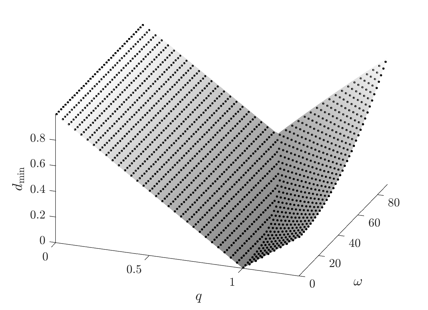
Figure 1: Comparison between the graph of $\max_{(e_{1},i_{1})}d_{\rm min}(q,\omega)$ defined in (31) and the maximum values of $d_{\rm min}$ computed with the algorithm of Section 3 for a grid of values of $(q_{1},\omega_{1})$.

To test our results also in case of two elliptic orbits, we consider the following bound introduced in [11] for the nodal distance $\delta_{\rm nod}$ defined below. Let

$$r =\frac{q_{1}(1+e_{1})}{1+e_{1}\cos\omega_{1}^{\scaleto{M}{3pt}}}, r_{\scaleto{-}{5pt}} =\frac{q_{1}(1+e_{1})}{1-e_{1}\cos\omega_{1}^{\scaleto{M}{3pt}}},$$

$$r_{\scaleto{+}{5pt}}^{\prime} =\frac{q_{2}(1+e_{2})}{1+e_{2}\cos\omega_{2}^{\scaleto{M}{3pt}}}, r_{\scaleto{-}{5pt}}^{\prime} =\frac{q_{2}(1+e_{2})}{1-e_{2}\cos\omega_{2}^{\scaleto{M}{3pt}}},$$

where $q_{2}$, $e_{2}$ are the pericenter distance and eccentricity of ${\cal A}_{2}$, and $\omega_{1}^{\scaleto{M}{3pt}}$, $\omega_{2}^{\scaleto{M}{3pt}}$ are the mutual arguments of pericenter (see [11]).

We introduce the ascending and descending nodal distances

$$d_{\rm nod}^{+}=r_{\scaleto{+}{5pt}}^{\prime}-r_{\scaleto{+}{5pt}},\qquad d_{\rm nod}^{-}=r_{\scaleto{-}{5pt}}^{\prime}-r_{\scaleto{-}{5pt}}.$$

The (minimal) nodal distance $\delta_{\rm nod}$ is defined as

$$\delta_{\rm nod}=\min\bigl{\{}|d_{\rm nod}^{+}|,|d_{\rm nod}^{-}|\bigr{\}}.$$ (33)

Set

$${\cal C}^{\prime}=[0,1]\times[0,\pi].$$

For each choice of $(q_{1},\omega_{1})\in{\cal D}$, defined as in (30), we have

$$\max_{(e_{1},\omega_{2}^{\scaleto{M}{3pt}})\in{\cal C}^{\prime}}\delta_{\rm nod}=\max\bigl{\{}u^{\omega}_{\rm int},u^{\omega}_{\rm ext},u^{\omega}_{\rm link}\bigr{\}},$$ (34)

where, denoting by $Q_{2}$ the apocenter distance of ${\cal A}_{2}$ and by $p_{2}=q_{2}(1+e_{2})$ its conic parameter,

$$u^{\omega}_{\rm int}(q,\omega)=p_{2}-q,$$

$$u^{\omega}_{\rm ext}(q,\omega)=\min\Bigl{\{}\frac{2q}{1-\cos\omega}-\frac{p_{2}}{1-\hat{\xi}^{\prime}_{*}},\ \frac{2q}{1+\cos\omega}-q_{2}\Bigr{\}},$$

$$u^{\omega}_{\rm link}(q,\omega)=\min\left\{Q_{2}-\frac{q(1+\hat{e}_{*})}{1+\hat{e}_{*}\cos\omega},\frac{2q}{1-\cos\omega}-q_{2}\right\},$$

with

$$\hat{\xi}^{\prime}_{*}=\min\{\xi_{*}^{\prime},e_{2}\},\qquad\xi^{\prime}_{*}(q,\omega)=\frac{4q\cos\omega}{p_{2}\sin^{2}\omega+\sqrt{p_{2}^{2}\sin^{4}\omega+16q^{2}\cos^{2}\omega}},$$

and

$$\hat{e}_{*}=\max\bigl{\{}0,\min\{e_{*},1\}\bigr{\}},$$

$$e_{*}(q,\omega)=\frac{2(p_{2}-q(1-e_{2}^{2}))}{q(1-e_{2}^{2})+\sqrt{q^{2}(1-e_{2}^{2})^{2}+4p_{2}\cos^{2}\omega(p_{2}-q(1-e_{2}^{2}))}}.$$

We compare the computed values of $d_{\rm min}$ with the bound (34) on the maximum nodal distance. The results are displayed in Figure 2 where, for four different values of $e_{2}$, the grey surface represents the bound of [11], while the black dots correspond to the maximum value of $d_{\rm min}$ for a grid in the $(q_{1},\omega_{1})$ plane computed with the method OE. Since the value of $\delta_{\rm nod}$ is always greater than or equal to the value of $d_{\rm min}$, for the test to be satisfied, we need all the black dots to fall below or lie on the grey surface. From Figure 2 we see that this is indeed what happens.

Similar checks done with the methods OT, OE, OES, TT, TTS were successful.

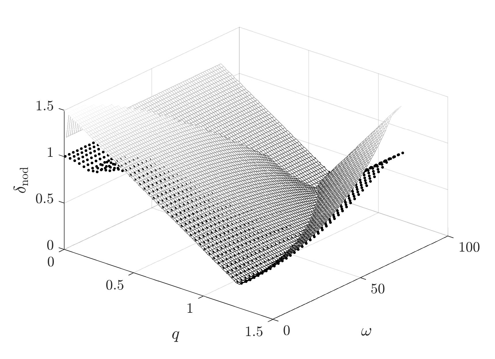
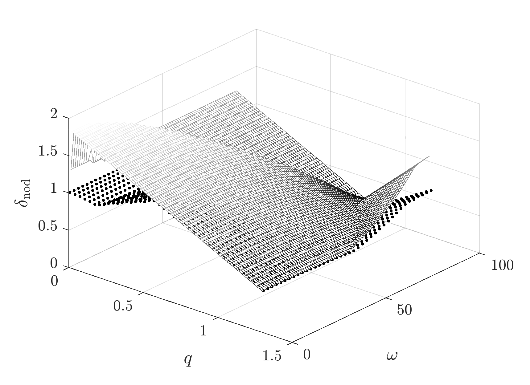
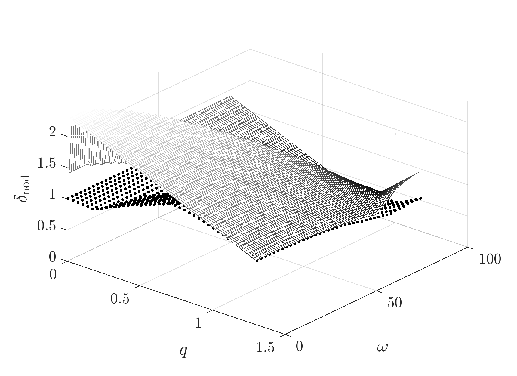
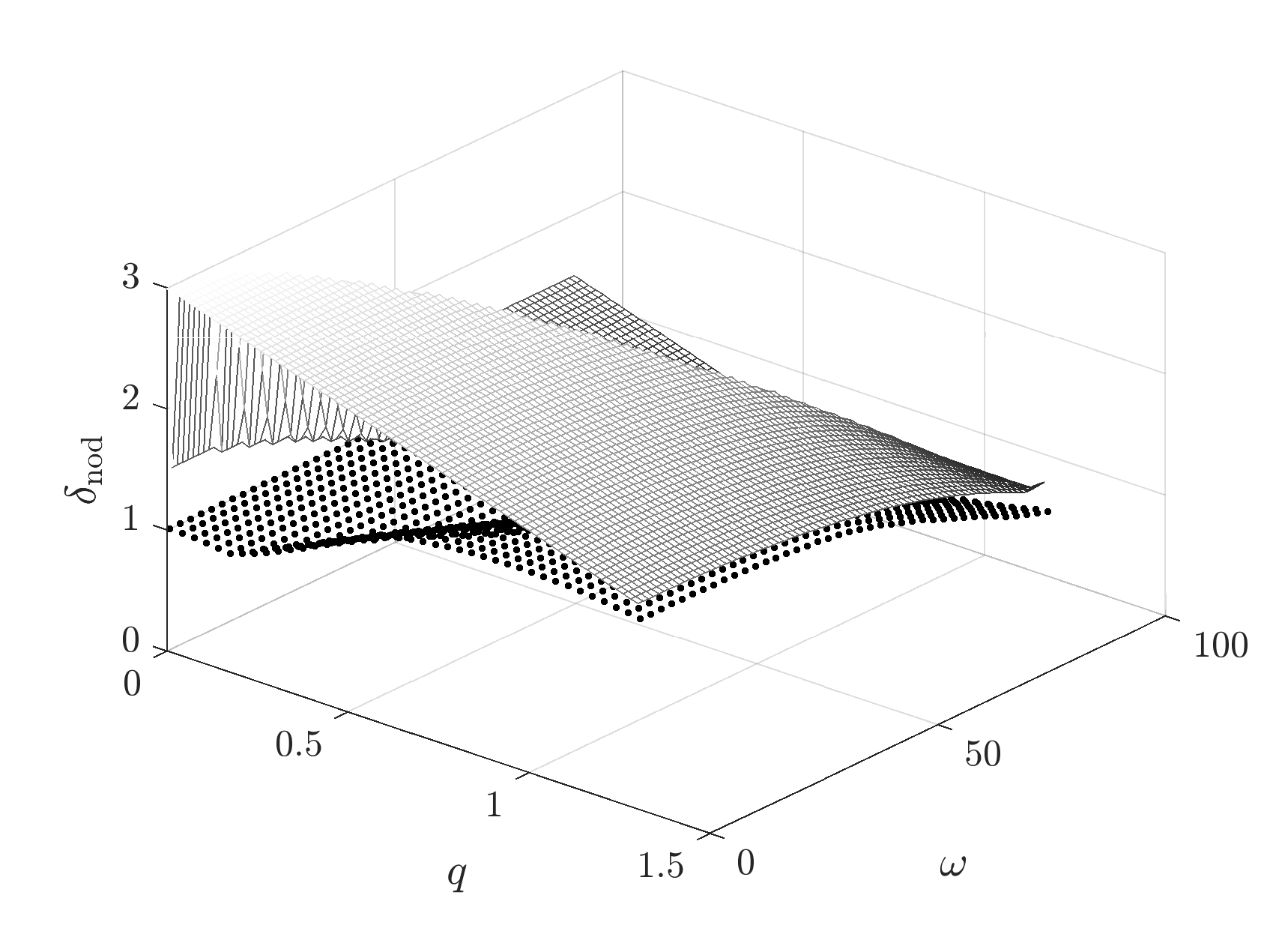
Figure 2: Comparison of the maximum MOID obtained with the method of Section 3 and the bound on the nodal distance found in [11]. These plots were drawn using values of $e_{2}$ equal to 0.2 (top-left), 0.3 (top-right), 0.4 (bottom-left) and 0.5 (bottom-right).

7 The planar case

Let us consider the case of two coplanar conics parametrized by the true anomalies $f_{1}$, $f_{2}$. Then, $(f_{1},f_{2})$ is a critical point of $d^{2}$ iff $d^{2}(f_{1},f_{2})=0$ or the tangent vectors

$$\bm{\tau}_{1}(f_{1})=\frac{\partial{\cal X}_{1}}{\partial f_{1}},\qquad\bm{\tau}_{2}(f_{2})=\frac{\partial{\cal X}_{2}}{\partial f_{2}}$$

to the first and second conic at ${\cal X}_{1}(f_{1})$ and ${\cal X}_{2}(f_{2})$, respectively, are parallel. If one trajectory, say the second one, is circular, then the tangent vector $\bm{\tau}_{2}$ is orthogonal to the position vector ${\cal X}_{2}$ for any value of $f_{2}$. Therefore, to find critical points that do not correspond to trajectory intersections, it is enough to look for values of $f_{1}$ such that $\mathbf{r}_{1}\cdot\bm{\tau}_{1}=0$. By symmetry, we can write

$${\cal X}_{1}=\begin{pmatrix}r_{1}\cos f_{1}\\ r_{1}\sin f_{1}\end{pmatrix},\qquad\text{with}\quad r_{1}=\frac{p_{1}}{1+e_{1}\cos f_{1}},$$

that is we can assume $\omega_{1}=0$. Thus, up to a multiplicative factor, we have

$$\bm{\tau}_{1}=\begin{pmatrix}-\sin f_{1}\\ \cos f_{1}+e_{1}\end{pmatrix},$$

so that

$$\mathbf{r}_{1}\cdot\bm{\tau}_{1}=\frac{p_{1}e_{1}\sin f_{1}}{1+e_{1}\cos f_{1}}=0$$

is satisfied iff $f_{1}=0,\pi$. Therefore, in general, we have the four critical points

$$(\bar{f}_{1},\bar{f}_{2})=(0,0),(0,\pi),(\pi,0),(\pi,\pi).$$

We may have at most two additional critical points that correspond to trajectory intersections, see [12, Sect. 7.1]. In conclusion, the maximum number of critical points with a circular and an elliptic trajectory in the planar case is 6.

We consider now the case of two ellipses. The position vectors can be written as

$${\cal X}_{1}=\begin{pmatrix}r_{1}\cos f_{1}\\ r_{1}\sin f_{1}\end{pmatrix},\qquad\text{with}\quad r_{1}=\frac{p_{1}}{1+e_{1}\cos f_{1}}$$

and

$${\cal X}_{2}=\begin{pmatrix}r_{2}\cos(f_{2}+\omega_{2})\\ r_{2}\sin(f_{2}+\omega_{2})\end{pmatrix},\qquad\text{with}\quad r_{2}=\frac{p_{2}}{1+e_{2}\cos f_{2}}.$$

Up to a multiplicative factor, we have

$$\bm{\tau}_{1}=\begin{pmatrix}-\sin f_{1}\\ \cos f_{1}+e_{1}\end{pmatrix},\hskip 28.45274pt\bm{\tau}_{2}=\begin{pmatrix}-\sin(f_{2}+\omega_{2})-e_{2}\sin\omega_{2}\\ \hphantom{+}\cos(f_{2}+\omega_{2})+e_{2}\cos\omega_{2}\end{pmatrix}.$$

The critical points that do not correspond to trajectory intersections are given by the values of $f_{1},f_{2}$ such that $\bm{\tau}_{1},\bm{\tau}_{2}$ are parallel and both orthogonal to ${\cal X}_{2}-{\cal X}_{1}$. These two conditions lead to the system

$$(\cos f_{1}+e_{1})[\sin(f_{2}+\omega_{2})+e_{2}\sin\omega_{2}]-\sin f_{1}[\cos(f_{2}+\omega_{2})+e_{2}\cos\omega_{2}]=0,$$ (35)

$$(\cos f_{1}+e_{1})[r_{2}\sin(f_{2}+\omega_{2})-r_{1}\sin f_{1}]-\sin f_{1}[r_{2}\cos(f_{2}+\omega_{2})-r_{1}\cos f_{1}]=0.$$ (36)

Multiplying (35) by $r_{2}$ and subtracting (36) we get

$$p_{1}e_{1}(1+e_{2}\cos f_{2})\sin f_{1}+p_{2}e_{2}(1+e_{1}\cos f_{1})(\cos f_{1}\sin\omega_{2}-\sin f_{1}\cos\omega_{2}+e_{1}\sin\omega_{2})=0.$$ (37)

Equations (35) and (37) can be written as

$$\alpha\cos f_{2}+\beta\sin f_{2}+\alpha e_{2}=0,$$ (38)

$$\mu\cos f_{2}+\delta=0,$$ (39)

$q$	$e$	$i$	$\Omega$	$\omega$
0.16582	0.84577	0	0	9.09466
1	0.2	0	0	10

Table 2: Cometary orbital elements of a pair of coplanar elliptic orbits giving 10 critical points. Angles are in degrees.

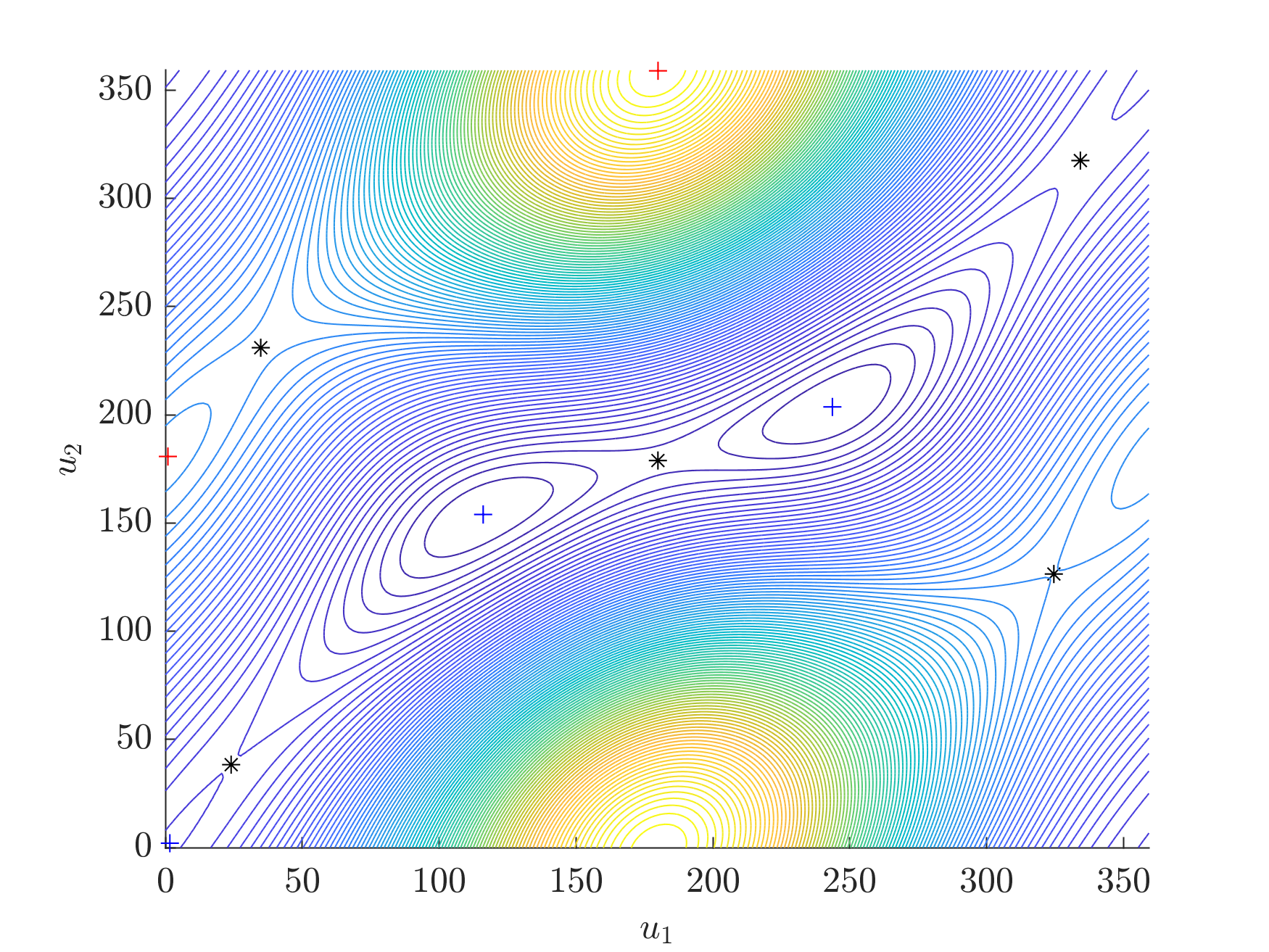
Figure 3: Level curves of the squared distance for the case reported in Table 2. The position of the critical points is highlighted: saddle points are represented by black asterisks, while the red and blue crosses correspond to maximum and minimum points, respectively.

$u_{1}$	$u_{2}$	$d$	Type
$116.0625325$	$153.9899286$	0.0000000	MINIMUM
$243.6382848$	$203.6865581$	0.0000000	MINIMUM
$179.8948964$	$178.9198966$	0.4845432	SADDLE
$1.6247542$	$2.0946456$	0.8341185	MINIMUM
$24.0090191$	$38.3799855$	0.8401907	SADDLE
$334.2162041$	$317.5202237$	0.8445898	SADDLE
$324.5270438$	$126.4762243$	1.6264123	SADDLE
$34.8254033$	$231.0377067$	1.6334795	SADDLE
$0.9077692$	$180.7796090$	1.6658557	MAXIMUM
$179.9346562$	$358.9929507$	2.9845260	MAXIMUM

Table 3: Critical points and critical values for the pair of orbits displayed in Table 2.

where

$$\alpha =\sin(\omega_{2}-f_{1})+e_{1}\sin\omega_{2},$$

$$\beta =\cos(\omega_{2}-f_{1})+e_{1}\cos\omega_{2},$$

$$\mu =p_{1}e_{1}e_{2}\sin f_{1},$$

$$\delta =p_{1}e_{1}\sin f_{1}+p_{2}e_{2}(1+e_{1}\cos f_{1})(\cos f_{1}\sin\omega_{2}-\sin f_{1}\cos\omega_{2}+e_{1}\sin\omega_{2}).$$

From (38) we obtain

$$\sin f_{2}=-\frac{\alpha}{\beta}(\cos f_{2}+e_{2}),$$

which is replaced into relation $\cos^{2}f_{2}+\sin^{2}f_{2}-1=0$ to give

$$(\alpha^{2}+\beta^{2})\cos^{2}f_{2}+2\alpha^{2}e_{2}\cos f_{2}+e_{2}^{2}\alpha^{2}-\beta^{2}=0.$$ (54)

Moreover, after replacing in (54)

$$\cos f_{2}=-\frac{\delta}{\mu},$$

which follows from (39), we obtain

$$(\alpha^{2}+\beta^{2})\delta^{2}-2e_{2}\alpha^{2}\delta\mu+\mu^{2}(e_{2}^{2}\alpha^{2}-\beta^{2})=0.$$ (55)

Since

$$\alpha^{2}+\beta^{2}=1+e_{1}^{2}+2e_{1}\cos f_{1},$$

the trigonometric polynomial in (55) has, in general, degree 5 in $\cos f_{1}$, $\sin f_{1}$. Therefore, we can not have more than 10 critical points which do not correspond to trajectory intersections. Then, the maximum number of critical points of $d^{2}$ (including intersections) for two elliptic orbits in the planar case is at most 12. However, we remark that this bound has never been reached in our numerical tests, where we got at most 10 critical points that we think is the maximum number. This conjecture adds a new question to Problem 8 in [1].

In Table 2 we write a set of orbital elements giving 10 critical points. We draw the level curves of $d^{2}$ in Figure 3, as function of the eccentric anomalies $u_{1},u_{2}$, where the position of each critical point is highlighted: we use an asterisk for saddle points, and crosses for local extrema. Finally, the critical points, the corresponding values of $d$ and their type (minimum, maximum, saddle) are displayed in Table 3.

8 Conclusions

In this work we investigate different approaches for the computation of the critical points of the squared distance function $d^{2}$, with particular care for the minimum values. We focus on the case of bounded trajectories. Two algebraic approaches are used: the first employs ordinary polynomials, the second trigonometric polynomials. In both cases we detail all the steps to reduce the problem to the computation of the roots of a univariate polynomial of minimal degree (that is 16, in the general case). The different methods are compared through numerical tests using the orbits of all the known near-Earth asteroids. We also perform some reliability tests of the results, which make use of known optimal bounds on the orbit distance. Finally, we improve the theoretical bound on the number of critical points in the planar case, and refine the related conjecture.

9 Acknowledgments

We wish to thank Leonardo Robol for his useful comments and suggestions. The authors have been partially supported through the H2020 MSCA ETN Stardust-Reloaded, Grant Agreement n. 813644. The authors also acknowledge the project MIUR-PRIN 20178CJA2B “New frontiers of Celestial Mechanics: theory and applications” and the GNFM-INdAM (Gruppo Nazionale per la Fisica Matematica).

Appendix A Coefficients of shifted polynomials for method with ordinary polynomials and eccentric anomalies

The coefficients of system (10) are

$$\tilde{\alpha} =\bigl{(}2(A_{1}-A_{3})\cos s_{1}\sin s_{1}-A_{10}\sin s_{1}-A_{11}\cos s_{1}+A_{12}\sin s_{1}+A_{8}\cos s_{1}\bigr{)}z^{4}$$

$$\quad\,+\bigl{(}-8(A_{1}-A_{3})\cos^{2}s_{1}+2A_{10}\cos s_{1}-2A_{11}\sin s_{1}\bigr{.}$$

$$\quad\,\bigl{.}{}-2A_{12}\cos s_{1}+2A_{8}\sin s_{1}+4(A_{1}-A_{3})\bigr{)}z^{3}-12(A_{1}-A_{3})\sin s_{1}\cos s_{1}z^{2}$$

$$\quad\,+\bigl{(}8(A_{1}-A_{3})\cos^{2}s_{1}+2A_{10}\cos s_{1}-2A_{11}\sin s_{1}-2A_{12}\cos s_{1}\bigr{.}$$

$$\quad\,\bigl{.}{}+2A_{8}\sin s_{1}-4(A_{1}-A_{3})\bigr{)}z+2(A_{1}-A_{3})\cos s_{1}\sin s_{1}$$

$$\quad\,+A_{10}\sin s_{1}+A_{11}\cos s_{1}-A_{12}\sin s_{1}-A_{8}\cos s_{1},$$

$$\tilde{\beta} =\left(-2A_{7}\cos s_{1}+2A_{9}\sin s_{1}\right)z^{4}+\left(-4A_{7}\sin s_{1}-4A_{9}\cos s_{1}\right)z^{3}$$

$$\quad\,+\left(-4A_{7}\sin s_{1}-4A_{9}\cos s_{1}\right)z+2A_{7}\cos s_{1}-2A_{9}\sin s_{1},$$

$$\tilde{\gamma} =\bigl{(}2(A_{1}-A_{3})\cos s_{1}\sin s_{1}+A_{10}\sin s_{1}-A_{11}\cos s_{1}+A_{12}\sin s_{1}-A_{8}\cos s_{1}\bigr{)}z^{4}$$

$$\quad\,+\bigl{(}-8(A_{1}-A_{3})\cos^{2}s_{1}-2A_{10}\cos s_{1}-2A_{11}\sin s_{1}\bigr{.}$$

$$\quad\,\bigl{.}{}-2A_{12}\cos s_{1}-2A_{8}\sin s_{1}+4(A_{1}-A_{3})\bigr{)}z^{3}-12(A_{1}-A_{3})\sin s_{1}\cos s_{1}z^{2}$$

$$\quad\,+\bigl{(}8(A_{1}-A_{3})\cos^{2}s_{1}-2A_{10}\cos s_{1}-2A_{11}\sin s_{1}-2A_{12}\cos s_{1}\bigr{.}$$

$$\quad\,\bigl{.}{}-2A_{8}\sin s_{1}-4(A_{1}-A_{3})\bigr{)}z+2(A_{1}-A_{3})\cos s_{1}\sin s_{1}$$

$$\quad\,-A_{10}\sin s_{1}+A_{11}\cos s_{1}-A_{12}\sin s_{1}+A_{8}\cos s_{1},$$

$$\tilde{A} =\left(A_{7}\sin s_{1}+A_{9}\cos s_{1}-A_{13}\right)z^{2}+\left(-2A_{7}\cos s_{1}+2A_{9}\sin s_{1}\right)z$$

$$\quad\,-A_{7}\sin s_{1}-A_{9}\cos s_{1}-A_{13},$$

$$\tilde{B} =\bigl{(}2A_{10}\cos s_{1}+2A_{8}\sin s_{1}-2A_{14}-4(A_{4}-A_{6})\bigr{)}z^{2}+\left(4A_{10}\sin s_{1}-4A_{8}\cos s_{1}\right)z$$

$$\quad\,-2A_{10}\cos s_{1}-2A_{8}\sin s_{1}-2A_{14}-4(A_{4}-A_{6}),$$

$$\tilde{D} =\bigl{(}2A_{10}\cos s_{1}+2A_{8}\sin s_{1}-2A_{14}+4(A_{4}-A_{6})\bigr{)}z^{2}+\left(4A_{10}\sin s_{1}-4A_{8}\cos s_{1}\right)z$$

$$\quad\,-2A_{10}\cos s_{1}-2A_{8}\sin s_{1}-2A_{14}+4(A_{4}-A_{6}).$$

Appendix B Factorization of $\mathscr{H}(f_{2})$

Let

$$\mathscr{T}=\left[\begin{array}[]{cccc}\alpha^{2}+\beta^{2}&0&\beta\kappa-\alpha\lambda&0\cr 2\alpha\gamma&\alpha^{2}+\beta^{2}&\beta\mu-\lambda\gamma-\alpha\nu&\beta\kappa-\alpha\lambda\cr\gamma^{2}-\beta^{2}&2\alpha\gamma&\beta\kappa-\gamma\nu&\beta\mu-\lambda\gamma-\alpha\nu\cr 0&\gamma^{2}-\beta^{2}&0&\beta\kappa-\gamma\nu\cr\end{array}\right]$$

and define

$$\mathscr{H}(f_{2})=\det\mathscr{T}.$$

Proposition 2.

We can extract the factor $\beta^{2}(1+e_{2}\cos f_{2})^{2}$ from $\det\mathscr{T}$.

Proof.

We first prove that we can extract the factor $\beta^{2}$.

Noting that

$$\kappa=\mu\eta,\qquad\eta=\frac{e_{1}}{1+e_{1}^{2}},$$ (56)

we consider

$$\mathscr{T}=\left[\begin{array}[]{cccc}\alpha^{2}+\beta^{2}&0&\beta\mu\eta-\alpha\lambda&0\cr 2\alpha\gamma&\alpha^{2}+\beta^{2}&\beta\mu-\lambda\gamma-\alpha\nu&\beta\mu\eta-\alpha\lambda\cr\gamma^{2}-\beta^{2}&2\alpha\gamma&\beta\mu\eta-\gamma\nu&\beta\mu-\lambda\gamma-\alpha\nu\cr 0&\gamma^{2}-\beta^{2}&0&\beta\mu\eta-\gamma\nu\cr\end{array}\right].$$

We can write $\det\mathscr{T}$ as a sum of terms where the only one that is independent on $\beta$ is

$$\left|\begin{array}[]{cccc}\alpha^{2}&0&-\alpha\lambda&0\cr 2\alpha\gamma&\alpha^{2}&-\lambda\gamma-\alpha\nu&-\alpha\lambda\cr\gamma^{2}&2\alpha\gamma&-\gamma\nu&-\lambda\gamma-\alpha\nu\cr 0&\gamma^{2}&0&-\gamma\nu\cr\end{array}\right|,$$

which is equal to $0$, as previously proved at the beginning of Proposition 1. The terms that are linearly dependent on $\beta$ are given by

$$\left|\begin{array}[]{cccc}\alpha^{2}&0&-\alpha\lambda&0\cr 2\alpha\gamma&\alpha^{2}&-\lambda\gamma-\alpha\nu&\beta\mu\eta\cr\gamma^{2}&2\alpha\gamma&-\gamma\nu&\beta\mu\cr 0&\gamma^{2}&0&\beta\mu\eta\cr\end{array}\right|,\hskip 28.45274pt\left|\begin{array}[]{cccc}\alpha^{2}&0&\beta\mu\eta&0\cr 2\alpha\gamma&\alpha^{2}&\beta\mu&-\alpha\lambda\cr\gamma^{2}&2\alpha\gamma&\beta\mu\eta&-\lambda\gamma-\alpha\nu\cr 0&\gamma^{2}&0&-\gamma\nu\cr\end{array}\right|,$$

and their sum is equal to $0$, because the two determinants are opposite. Therefore, $\mathscr{H}(f_{2})$ is made by terms of degree higher than 1 in $\beta$. Thus, we can write

$$\mathscr{H}(f_{2})=\mathfrak{D}_{1}+\mathfrak{D}_{2}+\mathfrak{D}_{3}+\mathfrak{D}_{4}+\mathfrak{D}_{5},$$

where

$$\mathfrak{D}_{1}=\left|\begin{array}[]{cccc}\beta^{2}&0&\beta\mu\eta&0\cr 0&\beta^{2}&\beta\mu&\beta\mu\eta\cr-\beta^{2}&0&\beta\mu\eta&\beta\mu\cr 0&-\beta^{2}&0&\beta\mu\eta\cr\end{array}\right|,$$

$$\mathfrak{D}_{2}=\left|\begin{array}[]{cccc}\beta^{2}&0&\beta\mu\eta&0\cr 0&\beta^{2}&\beta\mu&-\alpha\lambda\cr-\beta^{2}&0&\beta\mu\eta&-\lambda\gamma-\alpha\nu\cr 0&-\beta^{2}&0&-\gamma\nu\cr\end{array}\right|+\left|\begin{array}[]{cccc}\beta^{2}&0&-\alpha\lambda&0\cr 0&\beta^{2}&-\lambda\gamma-\alpha\nu&\beta\mu\eta\cr-\beta^{2}&0&-\gamma\nu&\beta\mu\cr 0&-\beta^{2}&0&\beta\mu\eta\cr\end{array}\right|,$$

$$\mathfrak{D}_{3} =\left|\begin{array}[]{cccc}\beta^{2}&0&-\alpha\lambda&0\cr 0&\beta^{2}&-\lambda\gamma-\alpha\nu&-\alpha\lambda\cr-\beta^{2}&0&-\gamma\nu&-\lambda\gamma-\alpha\nu\cr 0&-\beta^{2}&0&-\gamma\nu\cr\end{array}\right|+\left|\begin{array}[]{cccc}\alpha^{2}&0&\beta\mu\eta&0\cr 2\alpha\gamma&\beta^{2}&\beta\mu&\beta\mu\eta\cr\gamma^{2}&0&\beta\mu\eta&\beta\mu\cr 0&-\beta^{2}&0&\beta\mu\eta\cr\end{array}\right|$$

$$\quad\,+\left|\begin{array}[]{cccc}\beta^{2}&0&\beta\mu\eta&0\cr 0&\alpha^{2}&\beta\mu&\beta\mu\eta\cr-\beta^{2}&2\alpha\gamma&\beta\mu\eta&\beta\mu\cr 0&\gamma^{2}&0&\beta\mu\eta\cr\end{array}\right|,$$

$$\mathfrak{D}_{4} =\left|\begin{array}[]{cccc}\alpha^{2}&0&\beta\mu\eta&0\cr 2\alpha\gamma&\beta^{2}&\beta\mu&-\alpha\lambda\cr\gamma^{2}&0&\beta\mu\eta&-\lambda\gamma-\alpha\nu\cr 0&-\beta^{2}&0&-\gamma\nu\cr\end{array}\right|+\left|\begin{array}[]{cccc}\alpha^{2}&0&-\alpha\lambda&0\cr 2\alpha\gamma&\beta^{2}&-\lambda\gamma-\alpha\nu&\beta\mu\eta\cr\gamma^{2}&0&-\gamma\nu&\beta\mu\cr 0&-\beta^{2}&0&\beta\mu\eta\cr\end{array}\right|$$

$$\quad\,+\left|\begin{array}[]{cccc}\beta^{2}&0&\beta\mu\eta&0\cr 0&\alpha^{2}&\beta\mu&-\alpha\lambda\cr-\beta^{2}&2\alpha\gamma&\beta\mu\eta&-\lambda\gamma-\alpha\nu\cr 0&\gamma^{2}&0&-\gamma\nu\cr\end{array}\right|+\left|\begin{array}[]{cccc}\beta^{2}&0&-\alpha\lambda&0\cr 0&\alpha^{2}&-\lambda\gamma-\alpha\nu&\beta\mu\eta\cr-\beta^{2}&2\alpha\gamma&-\gamma\nu&\beta\mu\cr 0&\gamma^{2}&0&\beta\mu\eta\cr\end{array}\right|,$$

$$\mathfrak{D}_{5} =\left|\begin{array}[]{cccc}\alpha^{2}&0&-\alpha\lambda&0\cr 2\alpha\gamma&\beta^{2}&-\lambda\gamma-\alpha\nu&-\alpha\lambda\cr\gamma^{2}&0&-\gamma\nu&-\lambda\gamma-\alpha\nu\cr 0&-\beta^{2}&0&-\gamma\nu\cr\end{array}\right|+\left|\begin{array}[]{cccc}\beta^{2}&0&-\alpha\lambda&0\cr 0&\alpha^{2}&-\lambda\gamma-\alpha\nu&-\alpha\lambda\cr-\beta^{2}&2\alpha\gamma&-\gamma\nu&-\lambda\gamma-\alpha\nu\cr 0&\gamma^{2}&0&-\gamma\nu\cr\end{array}\right|$$

$$\quad\,+\left|\begin{array}[]{cccc}\alpha^{2}&0&\beta\mu\eta-\alpha\lambda&0\cr 2\alpha\gamma&\alpha^{2}&\beta\mu-\lambda\gamma-\alpha\nu&\beta\mu\eta-\alpha\lambda\cr\gamma^{2}&2\alpha\gamma&\beta\mu\eta-\gamma\nu&\beta\mu-\lambda\gamma-\alpha\nu\cr 0&\gamma^{2}&0&\beta\mu\eta-\gamma\nu\cr\end{array}\right|.$$

We have

$$\mathfrak{D}_{1} =\beta^{6}\mu^{2}(4\eta^{2}-1),$$

$$\mathfrak{D}_{2} =2\beta^{5}\mu\left[\lambda\gamma+\alpha\nu-2\eta(\alpha\lambda+\gamma\nu)\right],$$

$$\mathfrak{D}_{3} =\beta^{4}(\alpha^{2}-\gamma^{2})\left[\lambda^{2}-\nu^{2}+\mu^{2}(4\eta^{2}-1)\right],$$

$$\mathfrak{D}_{4} =-2\beta^{3}\mu\left[\gamma^{3}\lambda-\alpha^{3}\nu+\eta(\alpha^{3}\lambda-3\alpha\gamma^{2}\lambda+3\alpha^{2}\gamma\nu-\gamma^{3}\nu)\right],$$

$$\mathfrak{D}_{5} =\beta^{2}\mu^{2}\left[\alpha\gamma-\eta(\alpha^{2}+\gamma^{2})\right]^{2}-\beta^{2}(\alpha^{2}-\gamma^{2})(\lambda\gamma-\alpha\nu)^{2}.$$

Remark 1.

$\mathscr{H}(f_{2})/\beta^{2}$ is a trigonometric polynomial of degree 10 in $(\cos f_{2}$, $\sin f_{2})$.

Then, we show that $\xi^{2}=(1+e_{2}\cos f_{2})^{2}$ is a factor of $\mathscr{H}(f_{2})/\beta^{2}$. For this purpose, using the definitions of $\alpha$, $\beta$, $\nu$, $\lambda$, $\tilde{\alpha}$, $\tilde{\beta}$, $\tilde{\lambda}$ given in Section 5, we write

$$\alpha =\xi\tilde{\alpha}+e_{1}\gamma,$$ (85)

$$\beta =\xi\tilde{\beta},$$

$$\lambda =e_{1}\tilde{\lambda},$$ (86)

$$\nu =p_{1}e_{1}\xi+\tilde{\lambda}.$$ (87)

The factor $\beta^{2}$ can be extracted from $(\mathfrak{D}_{1}+\mathfrak{D}_{2}+\mathfrak{D}_{3})/\beta^{2}$, therefore also $\xi^{2}$ is a factor of this polynomial. Consider now $\mathfrak{D}_{4}/\beta^{2}$ and write it as

$$\mathfrak{D}_{4}/\beta^{2}=6\mu\beta\alpha\gamma(\gamma\lambda-\alpha\nu)-2\mu\beta\left[\lambda(\gamma^{3}+\eta\alpha^{3})-\nu(\alpha^{3}+\eta\gamma^{3})\right].$$

Noting that

$$\gamma\lambda-\alpha\nu=-\xi(\nu\tilde{\alpha}+p_{1}e_{1}^{2}\gamma)$$ (88)

and

$$\gamma^{3}\left[\lambda(1+\eta e_{1}^{3})-\nu(e_{1}^{3}+\eta)\right]=-\gamma^{3}(1+\eta e_{1}^{3})\xi p_{1}e_{1}^{2},$$

where we used the expressions of $\alpha$, $\lambda$, $\nu$ in (85), (86), (87) and the definition of $\eta$ in (56), we prove that $\xi^{2}$ factors $\mathfrak{D}_{4}/\beta^{2}$.

Finally, using relation (88) and

$$\alpha\gamma-\eta(\alpha^{2}+\gamma^{2})=\xi\tilde{\alpha}\left[\gamma(1-2\eta e_{1})-\xi\eta\tilde{\alpha}\right],$$

we show that also $\mathfrak{D}_{5}/\beta^{2}$ contains the factor $\xi^{2}$. ∎

The trigonometric polynomial

$$h(f_{2}) =\mathscr{H}(f_{2})/(\beta^{2}\xi^{2})$$

$$=\tilde{\beta}^{4}\xi^{2}\mu^{2}(4\eta^{2}-1)+2\tilde{\beta}^{3}\xi\mu\left[\lambda\gamma+\alpha\nu-2\eta(\alpha\lambda+\gamma\nu)\right]$$

$$\,\quad+\tilde{\beta}^{2}(\alpha^{2}-\gamma^{2})\left[\lambda^{2}-\nu^{2}+\mu^{2}(4\eta^{2}-1)\right]$$

$$\,\quad-2\mu\tilde{\beta}\tilde{\alpha}^{2}\xi^{2}\left[\tilde{\alpha}(\lambda\eta-\nu)-3\eta e_{1}^{3}p_{1}\gamma\right]+\mu^{2}\tilde{\alpha}^{2}\left[\gamma(1-2\eta e_{1})-\xi\eta\tilde{\alpha}\right]^{2}$$

$$\,\quad-2\mu\tilde{\beta}p_{1}e_{1}(1-e_{1}^{2})\eta\gamma^{2}\left[3e_{1}\tilde{\alpha}\xi-\gamma(1-e_{1}^{2})\right]-(\alpha^{2}-\gamma^{2})(\nu\tilde{\alpha}+p_{1}e_{1}^{2}\gamma)^{2}$$

is of degree 8 in $(\cos f_{2}$, $\sin f_{2})$.

Appendix C Angular shift for trigonometric polynomials

Let

$$p(x,y)=\sum_{(i,j)\in{\cal K}}p_{i,j}x^{i}y^{j},$$

with $x=\cos u,y=\sin u$ and ${\cal K}\subset\mathbb{N}\times\mathbb{N}$ (non-negative 2-index integers) be a trigonometric polynomial. We wish to write $p(x,y)$ in terms of the variables $(z,w)$, where

$$z=\cos v,\quad w=\sin v,\qquad v=u-\alpha,\quad\alpha\in\mathbb{R}.$$

Writing $c_{\alpha}$, $s_{\alpha}$ for $\cos\alpha$, $\sin\alpha$, respectively, we have

$$x=c_{\alpha}z-s_{\alpha}w,\qquad y=s_{\alpha}z+c_{\alpha}w,$$

so that we obtain

$$\begin{split}q(z,w)&=p(c_{\alpha}z-s_{\alpha}w,s_{\alpha}z+c_{\alpha}w)\\ &=\sum_{(i,j)\in{\cal K}}p_{i,j}\left[\sum_{h=0}^{i}\biggl{(}\begin{array}[]{c}i\cr h\end{array}\biggr{)}(c_{\alpha}z)^{h}(-s_{\alpha}w)^{i-h}\right]\left[\sum_{k=0}^{j}\biggl{(}\begin{array}[]{c}j\cr k\end{array}\biggr{)}(s_{\alpha}z)^{k}(c_{\alpha}w)^{j-k}\right]\\ &=\sum_{(i,j)\in{\cal K}}p_{i,j}\sum_{\ell=0}^{i+j}\sum_{h+k=\ell}\biggl{(}\begin{array}[]{c}i\cr h\end{array}\biggr{)}\biggl{(}\begin{array}[]{c}j\cr k\end{array}\biggr{)}(-1)^{i-h}(c_{\alpha})^{h+j-k}(s_{\alpha})^{i-h+k}z^{h+k}w^{i-h+j-k}\\ &=\sum_{(i,j)\in{\cal K}}p_{i,j}\sum_{\ell=0}^{i+j}\sum_{h=\max\{\ell-j,0\}}^{\min\{\ell,i\}}\biggl{(}\begin{array}[]{c}i\cr h\end{array}\biggr{)}\biggl{(}\begin{array}[]{c}j\cr\ell-h\end{array}\biggr{)}(-1)^{i-h}(c_{\alpha})^{2h+j-\ell}(s_{\alpha})^{i-2h+\ell}z^{\ell}w^{i+j-\ell}.\end{split}$$

If

$${\cal K}=\{0,1,\ldots,m\}\times\{0,1,\ldots,n\},$$

introducing the coefficients

$$C_{i,j,\ell}=\sum_{h=\max\{\ell-j,0\}}^{\min\{\ell,i\}}\biggl{(}\begin{array}[]{c}i\cr h\end{array}\biggr{)}\biggl{(}\begin{array}[]{c}j\cr\ell-h\end{array}\biggr{)}(-1)^{i-h}(c_{\alpha})^{2h+j-\ell}(s_{\alpha})^{i-2h+\ell},$$

we can write

$$\begin{split}q(z,w)&=\sum_{i=0}^{m}\sum_{j=0}^{n}p_{i,j}\sum_{\ell=0}^{i+j}C_{i,j,\ell}z^{\ell}w^{i+j-\ell}=\sum_{r=0}^{m+n}\sum_{i=\max\{r-n,0\}}^{\min\{r,m\}}p_{i,r-i}\sum_{\ell=0}^{\cancel{i}+r\cancel{-i}}C_{i,r-i,\ell}z^{\ell}w^{\cancel{i}+r\cancel{-i}-\ell}\\ &=\sum_{r=0}^{m+n}\sum_{\ell=0}^{r}q_{\ell,r-\ell}z^{\ell}w^{r-\ell},\end{split}$$

where

$$q_{\ell,r-\ell}=\sum_{i=\max\{r-n,0\}}^{\min\{r,m\}}p_{i,r-i}\,C_{i,r-i,\ell}.$$

References

• [1] A. Albouy, H. E. Cabral, and A. A. Santos. Some problems on the classical N-body problem. Celestial Mechanics and Dynamical Astronomy, 113(4):369–375, 2012.
• [2] C. A. Arroyo-Parejo, N. Sanchez-Ortiz, and R. Dominguez-Gonzalez. Effect of mega-constellations on collision risk in space. In 8th European Conference on Space Debris. ESA Space Debris Office, 2021.
• [3] R. V. Baluyev and K. V. Kholshevnikov. Distance Between Two Arbitrary Unperturbed Orbits. Celestial Mechanics and Dynamical Astronomy, 91(3-4):287–300, 2005.
• [4] D. A. Bini. Numerical computation of polynomial zeros by means of Aberth method. Numer. Algorithms, 13:179–200, 1997.
• [5] A. Casulli and L. Robol. Rank-structured QR for Chebyshev rootfinding. SIAM jour. of Matr. Anal. and Appl., 42(3):1148–1171, 2021.
• [6] D. Cox, J. Little, and D. O’Shea. Ideals, Varieties, and Algorithms. Springer-Verlag, 1992.
• [7] P. A. Dybczynski, T. J. Jopek, and R. A. Serafin. On the minimum distance between two Keplerian orbits with a common focus. Cel. Mech. Dyn. Ast., 38:345–356, 1986.
• [8] I. Good. The colleague matrix, a Chebyshev analogue of the companion matrix. Quart. J. Math. Oxford Ser. (2), 12:61–68, 1961.
• [9] G. F. Gronchi. On the stationary points of the squared distance between two ellipses with a common focus. SIAM Jour. Sci. Comp., 4(1):61–80, 2002.
• [10] G. F. Gronchi. An algebraic method to compute the critical points of the distance function between two Keplerian orbits. Cel. Mech. Dyn. Ast., 93(1):297–332, 2005.
• [11] G. F. Gronchi and L. Niederman. On the nodal distance between two Keplerian trajectories with a common focus. Cel. Mech. Dyn. Ast., 132(5):1–29, 2020.
• [12] G. F. Gronchi and G. Tommei. On the uncertainty of the minimal distance between two confocal keplerian orbits. Discrete and Continuous Dynamical Systems - B, 7(4):755–778, 2007.
• [13] G. F. Gronchi and G. B. Valsecchi. On the possible values of the orbit distance between a near-Earth asteroid and the Earth. Monthly Not. Royal. Astron. Soc., 429:2687–2699, 2013.
• [14] J. M. Hedo, M. Ruíz, and J. Peláez. On the minimum orbital intersection distance computation: a new effective method. MNRAS, 479(3):3288–3299, 2018.
• [15] K. V. Kholshevnikov and N. N. Vassiliev. On the distance function between two Keplerian elliptic orbits. Cel. Mech. Dyn. Ast., 75:75–83, 1999.
• [16] A. Milani, S. R. Chesley, P. W. Chodas, and G. B. Valsecchi. Asteroid Close Approaches: Analysis and Potential Impact Detection. In W. F. Bottke, Cellino A., Paolicchi P., and Binzel R. P., editors, ASTEROIDS III, pages 55–69. Arizona University Press, 2001.
• [17] A. Milani, S. R. Chesley, M. E. Sansaturio, G. Tommei, and G. B. Valsecchi. Nonlinear impact monitoring: line of variation searches for impactors. Icarus, 173(2):362–384, 2005.
• [18] V. Noferini and J. Pérez. Chebyshev rootfinding via computing eigenvalues. Math. of Comp., 86(306):1741–1767, 2017.
• [19] A. Rossi, A. Petit, and D. McKnight. Short-term space safety analysis of LEO constellations and clusters. Acta Astronautica, 175:476–483, 2020.
• [20] G. Sitarski. Approaches of the Parabolic Comets to the Outer Planets. Acta Astron., 18(2):171–195, 1968.
• [21] T. Wisniowski and H. Rickman. Fast Geometric Method for Calculating Accurate Minimum Orbit Intersection Distances (MOIDs). Acta Astronomica, 63:293–307, 2013.