Autonomous Control for Orographic Soaring of Fixed-Wing UAVs

Abstract

We present a novel controller for fixed-wing UAVs that enables autonomous soaring in an orographic wind field, extending flight endurance. Our method identifies soaring regions and addresses position control challenges by introducing a target gradient line (TGL) on which the UAV achieves an equilibrium soaring position, where sink rate and updraft are balanced. Experimental testing validates the controller’s effectiveness in maintaining autonomous soaring flight without using any thrust in a non-static wind field. We also demonstrate a single degree of control freedom in a soaring position through manipulation of the TGL.

I INTRODUCTION

UAVs have benefited from advancements in battery technology and miniaturization of avionics, which resulted in an increase in their endurance and range. However, the full potential of UAV applications remains limited by reduced flight time. Therefore, it is useful to research other techniques that can positively impact the effective endurance of these UAVs. An interesting technique that has shown great potential is exploiting updrafts to stay airborne nearly indefinitely. Albatrosses have perfected this technique of soaring [1, 2], allowing them to fly without mechanical energy cost and embark on journeys exceeding 20,000 km, staying airborne for multiple days at a time [3, 4].

All soaring techniques aim to extract sufficient energy to stay airborne without losing altitude. Dynamic soaring is when energy is extracted due to a gradient in the horizontal wind velocity [5], while static soaring relies on a vertical, upward wind component. Static soaring includes two types: thermal soaring, which is created by a rising column of air, and orographic soaring, which is created by the upwards deflection of the wind stream. This research focuses exclusively on orographic soaring.

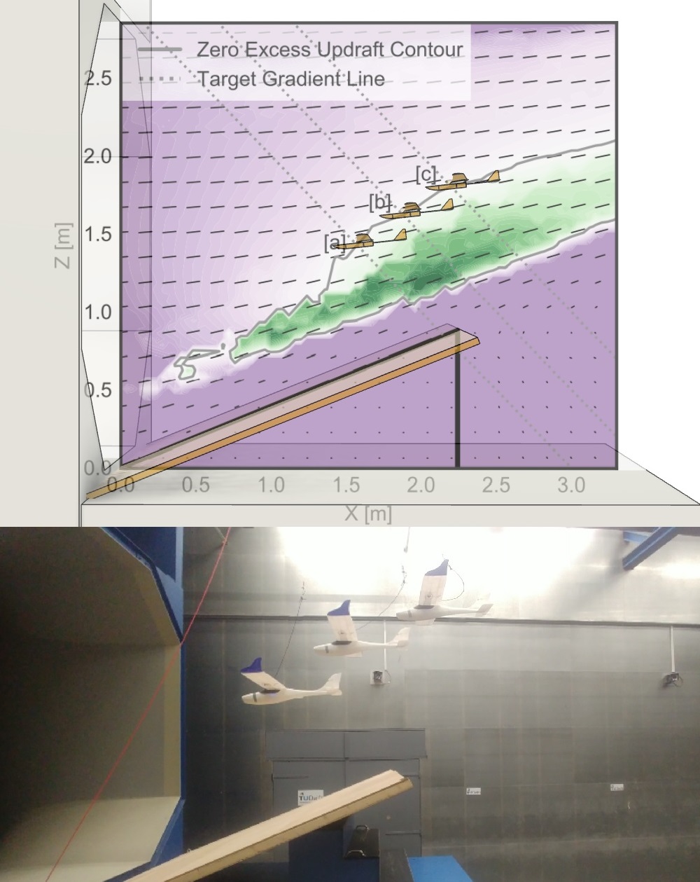
Figure 1: Autonomous soaring and position control of an UAV. The model shows the predicted excess updraft in the orographic wind field of the test setup. By precisely maintaining position control along an operator-specified target gradient line, the UAV successfully achieves autonomous soaring flight at the intersection with zero-excess updraft. The observed flight data, presented as three stacked stills in the image, correspond to the predicted soaring locations for three distinct target gradient lines specified in the test.

Prior research has explored the potential of exploiting orographic updrafts [6, 7, 8, 9, 10, 11]. White et al. utilized simulations and measurement data to evaluate the feasibility of soaring in the updraft generated by tall buildings. However, flight demonstrations were not conducted in these studies. While some studies have demonstrated orographic soaring [12, 13], they require a priori knowledge of the wind field and manual control of a human pilot to steer the UAV to an initial soaring position. Above studies considered a static wind field and predetermined path of the UAV.

In contrast, with this paper we propose a novel orographic soaring method with a single degree of control freedom, which can adapt to a non-static wind field, and does not require any throttle usage. Our method utilizes information derived from the approximate location of the updraft core but does not require complete prior knowledge of the wind field. We demonstrate fully autonomous soaring flight, and a single degree of position control of a UAV without propeller in a non-static wind field in a real-world test. We derive the kinematics involved with orographic soaring in section II. Its distinct control freedom is outlined in section III. Potential flow is used to estimate a soaring wind field in section IV. In section V, a control strategy is proposed to maintain autonomous soaring flight. The experimental test setup and test results are discussed in section VI and section VII.

II OROGRAPHIC SOARING

The kinematics involved with orographic soaring can be modeled using a point mass model, as illustrated by Langelaan [14]. In this model, we define the vehicle mass ($m$), angle of attack ($\alpha$), thrust ($T$), drag ($D$), and lift force ($L$) as key parameters.

First, considering the forces parallel and perpendicular to the flight path, we obtain two equations:

$$mg\cos(\gamma)=L+T\sin(\alpha)$$ (1)

$$mg\sin(\gamma)=D-T\cos(\alpha)$$ (2)

Here, flight path angle $\gamma$ is assumed small and a small angle approximation is used. Next, we obtain an equation that relates lift force to other parameters:

$$mg=L=\frac{1}{2}\rho v_{a}^{2}SC_{L}$$ (3)

Using this equation, we can calculate the lift coefficient ($C_{L}$) in terms of other parameters:

$$C_{L}=\frac{2mg}{\rho v_{a}^{2}S}$$ (4)

Additionally, we can derive a second-order approximation for the drag force ($D$):

$$D=\frac{1}{2}\rho v_{a}^{2}S(a_{0}+a_{1}C_{L}+a_{2}C_{L}^{2})$$ (5)

Substituting this approximation into Equation 2, we can calculate the flight path angle for a given speed and thrust:

$$mg\gamma=\frac{1}{2}\rho v_{a}^{2}(a_{0}+a_{1}C_{L}+a_{2}C_{L}^{2})-T$$ (6)

Finally, we can describe the aircraft kinematics in terms of airspeed, flight path angle, and wind speed. We define the horizontal ($\dot{x}_{i}$) and vertical ($\dot{z}_{i}$) velocity components in the inertial frame and model the wind speed as a polynomial function of position in the inertial frame ($w=f(x_{i},z_{i})$):

$$\dot{x}_{i}=v_{a}\cos(\gamma)+w_{x}$$ (7)

$$\dot{z}_{i}=v_{a}sin(\gamma)+w_{z}$$ (8)

III SOARING CONTROL FREEDOM

The ailerons, elevator, and rudder have a primary control effect on roll, pitch, and yaw respectively. Flight control in powered flight is further augmented by a throttle setpoint, which relates to the thrust reaction force. In the 6 degree of freedom (DOF) equations of motion, the aileron, elevator, rudder deflection, and thrust are the four main actuator control inputs. In this research it is useful to isolate the lateral and longitudinal motion.

Longitudinal motion:

$$\begin{split}&x=[\Delta u\;\;\Delta w\;\;\Delta q\;\;\Delta x\;\;\Delta z\;\;\Delta\theta]^{T}\\ &u=[\Delta\delta E\;\;\Delta\delta T]^{T}\end{split}$$ (9)

Lateral motion:

$$\begin{split}&x=[\Delta v\;\;\Delta p\;\;\Delta r\;\;\Delta y\;\;\Delta\phi\;\;\Delta\psi]^{T}\\ &u=[\Delta\delta A\;\;\Delta\delta R]^{T}\end{split}$$ (10)

For lateral motion, the dynamics during soaring remain the same. Therefore, the continuation of this report will focus solely on the longitudinal motion. As can be seen in Equation 9, in powered fixed-wing flight, elevator deflection and throttle setpoint are actuator inputs to the system. There are 6 state variables; position in the vertical plane, velocity in the vertical plane, pitch angle, and pitch rate.

Consider the available control freedom in the longitudinal motion of powered fixed-wing flight. Granted that the control objectives adhere to the nonholonomic constraints of the system, one is able to satisfy 2 of the 3 DOF. Fundamentally, this allows longitudinal control systems, such as a total energy control system to function [15]. Throttle and elevator control input are used to obtain a desired position and velocity in the vertical plane, resulting in pitch angle and pitch rate as dependent, uncontrollable variables.

The design of a soaring control strategy aims to eliminate throttle usage, leaving elevator deflection as the sole control actuator in the longitudinal motion. As a result, in this under-constrained system, traditional position control is not a viable option, and a novel approach is required.

IV WIND FIELD ANALYSIS

In the development of an orographic soaring control strategy, it is useful to consider methods to analyse and simulate a viable soaring wind field. A simplified potential flow model can be used for this, which estimates the wind field over an idealized hill with a semi-circular cross-section. [16, 17].

Potential flow around a cylinder can be obtained by considering a uniform stream of velocity $(U)$ and a doublet at the center of the cylinder such that the stagnation point precisely matches the boundary of the cylinder. The solution is most easily obtained in polar coordinates:

$$\Phi(r,\theta)=Ur(1\text{ -- }\frac{R^{2}}{r^{2}}cos(\theta))$$ (11)

The velocity in polar coordinates is then:

$$V_{r}=\frac{\delta\Phi}{\delta r}=U(1\text{ -- }\frac{R^{2}}{r^{2}}cos(\theta))$$ (12)

$$V_{\theta}=\frac{1}{r}\frac{\delta\Phi}{\delta\theta}=\text{ --}U(1+\frac{R^{2}}{r^{2}}sin(\theta))$$ (13)

This can be related to Cartesian coordinates by substituting $x=rcos(\theta)$ and $y=rsin(\theta)$.

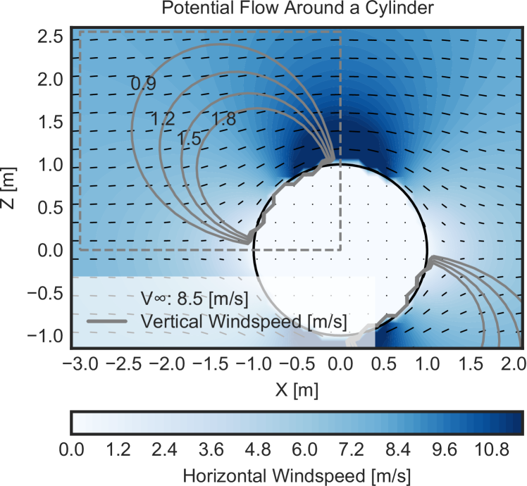
Figure 2: Wind velocity components around a cylinder obtained with potential flow theory. The upper windward quadrant is an orographic wind field.

The wind field is illustrated in Figure 2, which shows the upper windward quadrant as an orographic wind field. Of particular interest in the wind field is the vertical wind component, which should match the sink rate of the UAV to sustain soaring flight.

Therefore, for soaring flight it is useful to consider the glide polar of an airframe, as it precisely describes the relationship between airspeed and sink rate. At the maximum endurance speed ($V_{ME}$) a particular airframe will experience the lowest rate of sink. At lower velocities the airfoil will enter its stall regime and sink rate will increase. To maintain higher velocities than $V_{ME}$ during unpowered flight, the aircraft has to assume a nose-down attitude and the sink rate will increase as well. An arbitrary quadratic function that follows the characteristics of a glide polar is chosen to study its effect in an orographic soaring wind field.

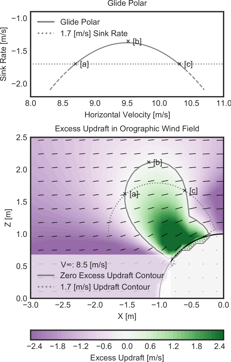
Figure 3: The glide polar defines the relation of the sink rate and horizontal velocity. Mapping of this glide polar on the orographic wind field yields the zero excess updraft contour. Three different soaring positions and their respective state on the glide polar are mapped.

As introduced by Fisher et al. [12], we can determine the feasible soaring region. At every point in the wind field, the local vertical updraft component is compared to the expected sink rate at the local horizontal wind velocity according to the glide polar. In this research we introduce the zero excess updraft contour (ZEUC); the line in the windfield where the expected local updraft equates the sink rate. The inner region defined by the ZEUC has an excess in updraft and the outer region has a lack of sufficient updraft. The process is illustrated in Figure 3. The aircraft is able to maintain its soaring position at every point on this contour. Three different soaring positions and their respective state on the glide polar are mapped. At $[a]$ and $[c]$, the aircraft will experience the same sink rate of $1.7m/s$ at a different horizontal velocity wind component, whereas in $[b]$ the aircraft requires the least updraft to maintain its soaring position.

V AUTONOMOUS CONTROL STRATEGY

As concluded in section III, the longitudinal motion of a soaring UAV is an under-actuated system. The feasible region where the UAV can soar efficiently in the vertical plane is limited to a specific contour line called zero excess updraft contour (ZEUC), as outlined in section IV. However, the location of this contour line cannot be determined without prior knowledge of the wind field, which complicates the use of a position controller. To address this issue, we introduce a target gradient line (TGL) as a novel approach to control the UAV’s position.

The TGL represents a path in the wind field along which there is a gradient in the available updraft. The TGL is chosen thoughtfully to originate at a point in the wind field where there exists excess updraft and extends upwards to a region of lack in updraft. The UAV utilizes its single degree of longitudinal control to maintain position on the TGL but is free to move along it. As a result, the UAV naturally settles in an equilibrium at the intersection of the TGL and ZEUC. This approach simplifies the control strategy, making it easier to implement and more robust to variations in the wind field.

The natural equilibrium soaring location of the UAV can be influenced by several factors. Firstly, the operator can manipulate the UAV’s position along the ZEUC by rotating or translating the TGL in the vertical plane, thereby realizing a single degree of control freedom. Secondly, during flight, small changes in the wind field are expected, which can result in a changing position of the ZEUC. By maintaining position on the TGL, The UAV will naturally move along the TGL to a new equilibrium point, which will be at the intersection with the ZEUC.

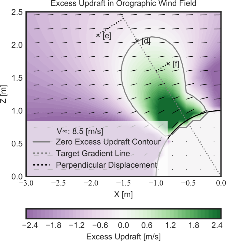
Figure 4: The autonomous control strategy considers a target gradient line intersecting the zero excess updraft contour. The controller response is proportional to the perpendicular displacement to the TGL.

The controller to maintain position on the TGL is implemented as a closed-loop pitch controller. The perpendicular distance of the UAV to the TGL, $(e_{\rho})$, is formulated as an error input for the controller. By convention, $e_{\rho}$ is positive when the UAV is upstream of the TGL and negative when the UAV is downstream, defined in Equation 14.

$$e_{\rho}=s*\frac{\mid Ax_{1}+Bz_{1}+C\mid}{A^{2}+B^{2}}\quad\text{with }\quad\begin{aligned} s&=\hskip 7.59995pt1\text{ IF upstream}\\ s&=-1\text{ IF downstream}\end{aligned}$$ (14)

With $TGL:Ax+Bz+C=0$ and UAV position $P:(x_{1},z_{1})$. The implementation is the test setup is analogous, where instead the TGL is extruded along $y$, and the perpendicular distance to said target plane is considered.

The pitch setpoint is then obtained as follows:

$$\theta_{sp}=\theta_{0}+k_{p}e_{\rho}+k_{i}\int e_{\rho}dt+k_{d}\frac{de_{\rho}}{dt}$$ (15)

$\theta_{0}$ is the trimmed pitch angle at the expected flight velocity. Stable soaring flight can be achieved by tuning the proportional ($k_{p}$) and derivative ($k_{d}$) gains. The use of an integral gain ($k_{i}$) is recommended to minimise steady-state error and realise full convergence to the TGL. The elevator setpoint $(e_{sp})$ is controlled with a closed-loop controller, taking as input the pitch error $(\theta_{e})$.

$$e_{sp}=k_{p}\theta_{e}+k_{i}\int\theta_{e}dt+k_{d}\frac{d\theta_{e}}{dt}$$ (16)

The TGL can be thoughtfully chosen to best deal with disturbances to the equilibrium. Namely, the total energy state of the vehicle in immediate proximity to the TGL should be considered. For instance, a horizontal TGL would often be a poor choice. A vehicle that finds itself below the TGL might lack the potential energy as well as higher updraft regions to regain altitude towards its TGL. Furthermore, a TGL is best chosen roughly perpendicular to the ZEUC. This way, minimal displacement along the TGL is required to accommodate changes in the wind field. It is important to note that this control strategy does not require a priori knowledge of the wind field. However, a general estimate of the shape of the wind field, such as knowledge of the location of the updraft core, is desired to effectively choose a TGL.

VI EXPERIMENTAL TEST SETUP

We conducted a full-scale test campaign in the open jet facility at Delft University of Technology. The facility has an outlet cross-section of $2.85m$ and can generate wind velocities up to $35m/s$. An updraft was created by placing a board at various angles in the airflow. We used this geometry to create a CFD model to estimate wind velocity components in the test section at various wind velocities and slope positions. [18]. The geometry is highlighted in Figure 1 and the velocity components are shown in Figure 5.

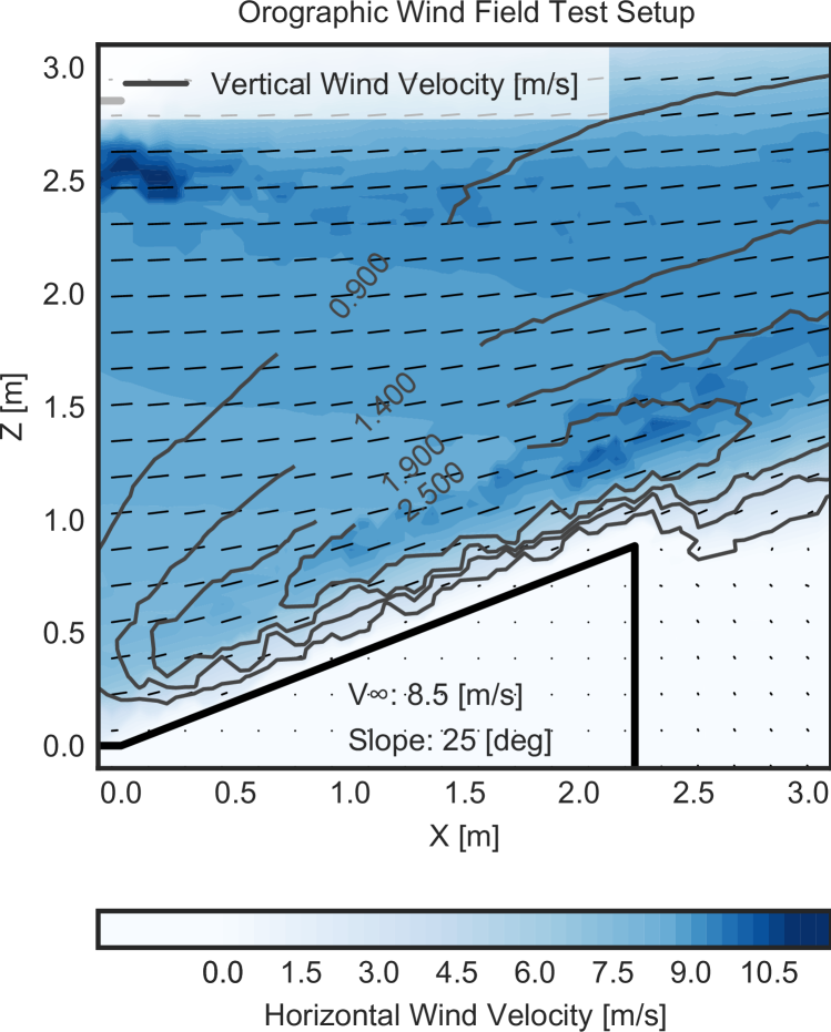
Figure 5: Wind velocity components of the orographic wind field in the experimental test setup, obtained by CFD.

The test UAV was a modified Eclipson Model C [19] 3D-printed model aircraft running Paparazzi autopilot [20]. The aircraft had three degrees of actuation with aileron, rudder, and elevator but no propeller. We determined the aircraft’s glide polar by third-order polynomial regression of gliding flight data at discretely different pitch attitudes. This glide polar is shown in Figure 7. We used an Optitrack system [21], mounted in the test facility, to receive the aircraft’s positioning data, which was also logged to evaluate the controller’s performance. An image of the test setup and its components is shown in Figure 6.

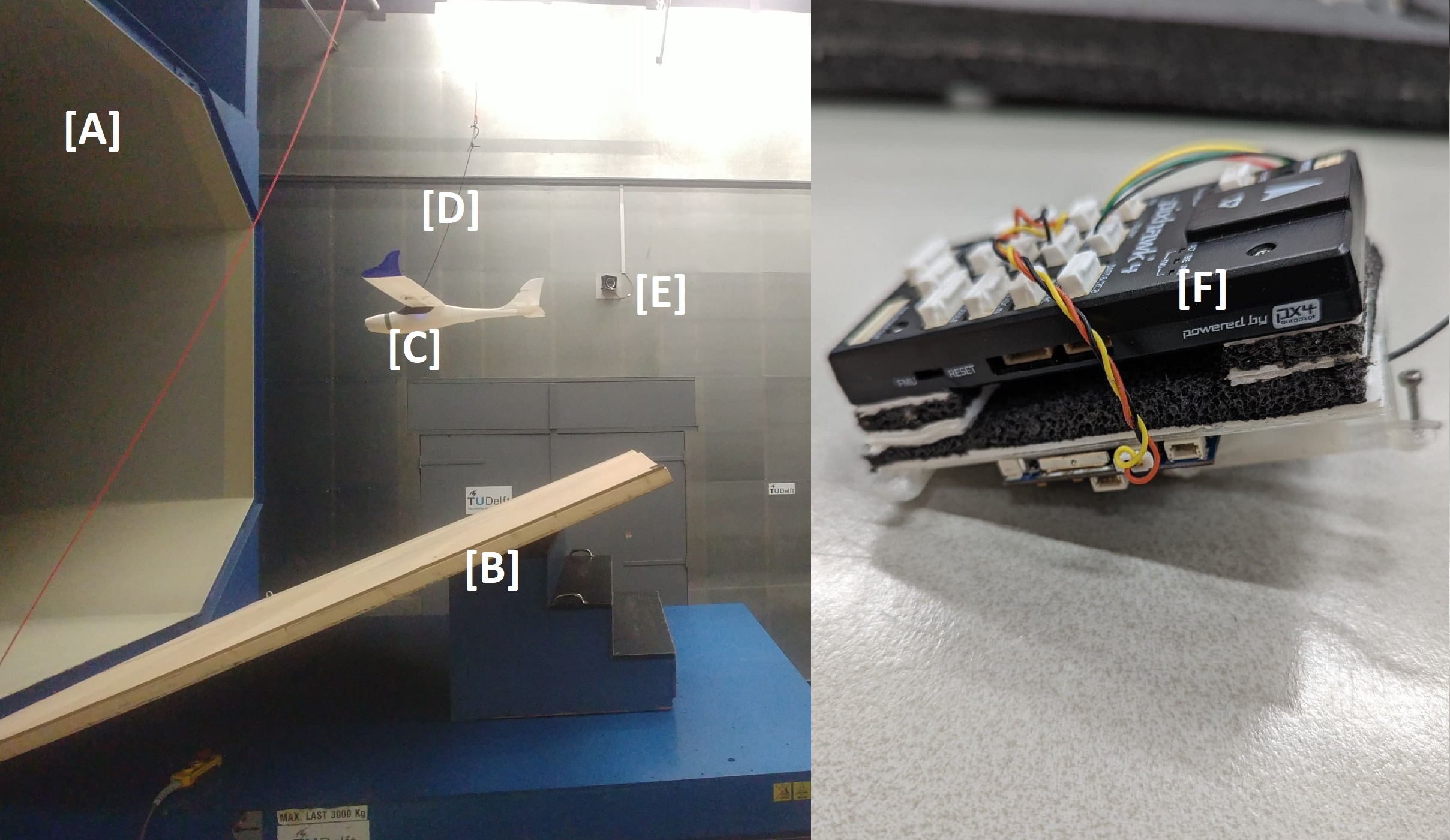
Figure 6: Test setup and data collection. [A] Open Jet Facility wind tunnel, [B] Adjustable slope, [C] UAV (without propeller mounted), [D] Safety tether, [E] Optitrack system camera, [F] Pixhawk 4 running Paparazzi autopilot

To ensure lateral stability and heading during testing, we implemented two lateral closed-loop control systems. The roll controller affects the ailerons and keeps the aircraft level, while the yaw controller affects the rudder and maintains the heading towards a virtual waypoint located $5m$ upwind from the wind tunnel settling chamber, achieving centering within the wind tunnel cross-section. The yaw error is defined as $e_{\psi}=\tan(y/R)-\psi$, where $y$ is the displacement from the vertical center plane in the wind tunnel and $R$ is the distance to the virtual upwind waypoint.

Both actuator setpoints are obtained through a closed-loop control system with proportional ($k_{p}$), integral ($k_{i}$), and derivative ($k_{d}$) gains, as shown in Equations 17 and 18. The novel soaring controller, presented in section V, affects the elevator.

$$a_{sp}=k_{p}e_{\phi}+k_{i}\int e_{\phi}dt+k_{d}\frac{de_{\phi}}{dt}$$ (17)

$$r_{sp}=k_{p}e_{\psi}+k_{d}\frac{de_{\psi}}{dt}$$ (18)

Our primary goal was to validate the novel soaring controller and investigate the effect of changing the slope, wind speed, and placement of the TGL.

VII TEST RESULTS AND DISCUSSION

By combining the velocity components in the wind field from CFD simulations and the glide polar, the (ZEUC) can be generated, as shown in Figure 7. It should be noted that the required updraft along the ZEUC is not a constant amount. It is a function of the local horizontal wind velocity component and the glide polar.

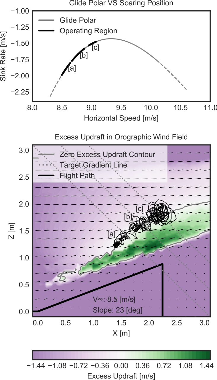
Figure 7: Mapping of the Eclipson Model C glide polar on the orographic wind field of the experimental test setup, yielding the expected zero excess updraft contour. Three different TGL positions are tested and the corresponding flight path is plotted. Note that the flight path corresponds well with the expected soaring locations.

In Figure 7, consider a test with the leftmost static TGL at position $[a]$. After manual tuning of the controller gains, it is observed from the flight path that the controller is able to successfully maintain position with minimal oscillations. Note that the TGL was chosen to be roughly perpendicular to the ZEUC. Defining a TGL less perpendicular to the ZEUC negatively affected the controller performance with larger oscillations and drift from the TGL.

As we translate the TGL to positions $[b]$ and $[c]$, the settled equilibrium of the aircraft also moves along with the TGL. Each equilibrium point corresponds to a different part of the aircraft’s glide polar. Notably, the flight path positions recorded during the test closely coincide with the intersection of the TGL and ZEUC. This confirms the effectiveness of the controller in maintaining position on the chosen TGL and the accuracy of the estimated wind field and glide polar. Additionally, moving the TGL proves to be an effective method for achieving a single degree of position control freedom with this soaring controller. Larger oscillations were observed downstream as a result of overshoot due to the increased elevator effectiveness at higher airspeed.

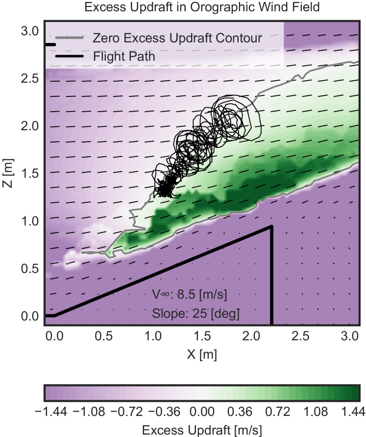
Figure 8: Effect of changing the slope from $23deg$ to $25deg$. The zero excess updraft contour (ZEUC) is now located noticeably higher. The flight path is plotted over a translating TGL. From the flight track we observe that the soaring location corresponds with the newly obtained ZEUC.

In Figure 8, we investigated the effect of changing the slope in the test setup on the resultant ZEUC. We increased the slope from $23$ to $25$ degrees and observed that the contour shifted upwards. To study the controller’s adaptability to changes in the wind field, we repeated the testing with incremental translation of the TGL at this higher slope. Our results show that the controller was able to adapt to changes in the wind field while maintaining the same level of control freedom.

Next, we examined the effect of changes in wind speed on the UAV’s performance. We incrementally increased the wind speed from $8.5$ to $9.5$ m/s while maintaining the same TGL. Throughout this range, the UAV was able to successfully maintain soaring flight, and we did not observe any significant changes in its hovering position. This unexpected result can be explained by considering the immediate effect of changes in horizontal wind velocity on the updraft and sink rate. We assumed that the vertical updraft component would scale proportionally to the horizontal wind. Therefore, a change in wind velocity would not change the shape of the wind field, but it would only scale the magnitude of all local wind vectors.

Consider Figure 9, which presents three scenarios where the updraft and sink rate are initially balanced.

• In scenario [a], the airfoil is in the stall regime and a change in wind velocity has a significant impact on the updraft and sink rate. An increase in wind velocity leads to an increase in the updraft component and a decrease in the sink rate, resulting in a net upward movement. Conversely, a decrease in wind velocity causes a net downward movement.

• In scenario [c], a change in wind velocity has a greater impact on the sink rate than the updraft, leading to a net downward movement with an increase in wind velocity and a net upward movement with a decrease in wind velocity.

• Finally, when the aircraft is operating near its optimal glide speed in the vicinity of [b], changes in wind velocity cause both the updraft and sink rate to change at a comparable rate, resulting in minimal movement. This scenario was observed during the experimental test and helps explain that limited movement was observed.

A change in wind velocity alters the shape and position of the ZEUC accordingly. The reaction force resulting from an imbalance between updraft and sink rate allows the aircraft to settle on the newly obtained ZEUC.

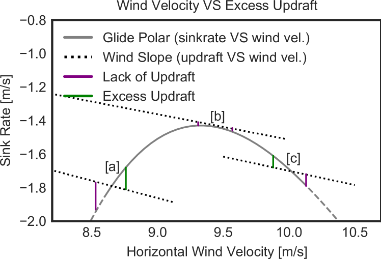
Figure 9: Comparison of the immediate change in sink rate and updraft as a result of changing the horizontal wind velocity at different segments on the glide slope. Changes in wind velocity affect the generated updraft in the wind field and effective sink rate of the aircraft differently.

VIII CONCLUSIONS

The objective of this research was to demonstrate the feasibility of autonomous orographic soaring for fixed-wing UAVs. We identified the feasible soaring region, which can be represented by a single line known as the zero excess updraft contour (ZEUC).

As the longitudinal motion of a soaring UAV is an under-actuated system, we introduced the concept of a target gradient line (TGL) to provide a single degree of control freedom. We then presented an autonomous controller that enables position keeping at the intersection of the TGL and ZEUC. We validated the controller in an experimental test setup, and the results showed that it effectively maintained position on the chosen TGL without using any thrust as the UAV had no propeller. Furthermore, the position of the logged flight segments closely aligned with the expected ZEUC, which was derived from the estimated wind field and glide polar.

We demonstrated that adjusting the TGL is an effective way to realize a single degree of control freedom in the system. Finally, we showed that the controller is robust to changes in the wind field, such as alterations in slope or changes in the free-stream velocity of the wind tunnel.

The performed tests in this research were limited by the cross-section of the wind tunnel. To enable a larger orographic wind field and more diverse wind conditions, additional testing in an outdoor environment is recommended. Furthermore, this would enable testing in a wider envelope of the UAV’s glide polar. When soaring in a broad airspeed range, it is recommended to adjust the gains for changes in elevator effectiveness. Finally, it can be challenging to set a favorable TGL without a priori knowledge of the wind field. Further research on obtaining an initial soaring position is suggested.

References

- [1] L. Rayleigh, “The soaring of birds,” Nature, vol. 27, no. 701, pp. 534–535, 1883.
- [2] J. Rayleigh, “The sailing flight of the albatross,” Nature, vol. 40, no. 1019, p. 34, 1889.
- [3] H. Weimerskirch, K. Delord, A. Guitteaud, R. A. Phillips, and P. Pinet, “Extreme variation in migration strategies between and within wandering albatross populations during their sabbatical year and their fitness consequences,” Scientific reports, vol. 5, no. 1, pp. 1–7, 2015.
- [4] G. Sachs, J. Traugott, A. P. Nesterova, G. Dell’Omo, F. Kümmeth, W. Heidrich, A. L. Vyssotski, and F. Bonadonna, “Flying at no mechanical energy cost: disclosing the secret of wandering albatrosses,” 2012.
- [5] Y. J. Zhao, “Optimal patterns of glider dynamic soaring,” Optimal control applications and methods, vol. 25, no. 2, pp. 67–89, 2004.
- [6] C. White, E. W. Lim, S. Watkins, A. Mohamed, and M. Thompson, “A feasibility study of micro air vehicles soaring tall buildings,” Journal of Wind Engineering and Industrial Aerodynamics, vol. 103, pp. 41–49, 2012.
- [7] C. White, S. Watkins, E. W. Lim, and K. Massey, “The soaring potential of a micro air vehicle in an urban environment,” International Journal of Micro Air Vehicles, vol. 4, no. 1, 2012.
- [8] A. Mohamed, R. Carrese, D. Fletcher, and S. Watkins, “Scale-resolving simulation to predict the updraught regions over buildings for mav orographic lift soaring,” Journal of Wind Engineering and Industrial Aerodynamics, vol. 140, pp. 34–48, 2015.
- [9] A. Mohamed, M. Abdulrahim, S. Watkins, and R. Clothier, “Development and flight testing of a turbulence mitigation system for micro air vehicles,” Journal of Field Robotics, vol. 33, no. 5, 2016.
- [10] A. Guerra-Langan, S. Araujo-Estrada, and S. Windsor, “Unmanned aerial vehicle control costs mirror bird behaviour when soaring close to buildings,” International Journal of Micro Air Vehicles, vol. 12, p. 1756829320941005, 2020.
- [11] J. W. Langelaan, N. Alley, and J. Neidhoefer, “Wind field estimation for small unmanned aerial vehicles,” Journal of Guidance, Control, and Dynamics, vol. 34, no. 4, 2011.
- [12] A. Fisher, M. Marino, R. Clothier, S. Watkins, L. Peters, and J. L. Palmer, “Emulating avian orographic soaring with a small autonomous glider,” Bioinspiration & biomimetics, vol. 11, no. 1, p. 016002, 2015.
- [13] C. P. de Jong, B. D. Remes, S. Hwang, and C. De Wagter, “Never landing drone: Autonomous soaring of a unmanned aerial vehicle in front of a moving obstacle,” International Journal of Micro Air Vehicles, vol. 13, p. 17568293211060500, 2021.
- [14] J. Langelaan, “Long distance/duration trajectory optimization for small uavs,” in AIAA guidance, navigation and control conference and exhibit, 2007, p. 6737.
- [15] A. A. Lambregts, “TECS generalized airplane control system design – an update,” in Advances in Aerospace Guidance, Navigation and Control. Springer Berlin Heidelberg, 2013, pp. 503–534.
- [16] J. D. Anderson, “Fundamentals of aerodynamics,” McGraw, 2009.
- [17] M. Gossye, S. Hwang, and B. Remes, “Developing a modular tool to simulate regeneration power potential using orographic wind-hovering uavs,” Unmanned Systems, 2022.
- [18] ANSYS, “Ansys® academic research fluent, release 19.5.0,” 2019.
- [19] Eclipson. 3d printed airplanes. [Online]. Available: https://www.eclipson-airplanes.com/modelc
- [20] G. Hattenberger, M. Bronz, and M. Gorraz, “Using the paparazzi uav system for scientific research,” 2014.
- [21] Optitrack. Motion capture systems. [Online]. Available: http://www.optitrack.com/