Generalized Expectation Maximization Framework for Blind Image Super Resolution

Abstract

Learning-based methods for blind single image super resolution (SISR) conduct the restoration by a learned mapping between high-resolution (HR) images and their low-resolution (LR) counterparts degraded with arbitrary blur kernels. However, these methods mostly require an independent step to estimate the blur kernel, leading to error accumulation between steps. We propose an end-to-end learning framework for the blind SISR problem, which enables image restoration within a unified Bayesian framework with either full- or semi-supervision. The proposed method, namely SREMN, integrates learning techniques into the generalized expectation-maximization (GEM) algorithm and infers HR images from the maximum likelihood estimation (MLE). Extensive experiments show the superiority of the proposed method with comparison to existing work and novelty in semi-supervised learning.

Index Terms—  Blind SISR, blur kernel, Bayesian model, GEM algorithm, semi-supervision.

1 Introduction

Single image super resolution (SISR) refers to the restoration of the plausible and detailed high-resolution (HR) image from the corresponding low-resolution (LR) image, with a wide range of applications [1, 2]. A widely-adopted model for SISR is as a degradation process where the LR image is a blurred, decimated, and noisy version of its HR counterpart [3, 4]. Since real-world distributions of these variables are difficult to access, restoring HR images is a classic ill-posed, inverse problem without a closed-form solution.

Learning-based methods for SISR represent to be a popular trend due to their superiority in dealing with complicated manifold-like image distributions. Pioneered by SRCNN [5], these methods learn the mapping between LR and HR image pairs with developed neural networks, such as residual networks (ResNets) [6] and generative adversarial networks (GANs) [7]. However, existing works typically synthesize LR images via a bicubic degradation model, and cannot generalize well to practical cases with complicated degradation settings.

Recently, learning-based methods for blind SISR has been proposed to address such problem [8, 9, 10]. Most works decompose SISR into two sequential steps, and independently estimate the blur kernel from LR images before inferring the HR images [11, 12, 13]. Such separation of kernel estimation and HR image restoring may not be compatible and result in error accumulation. [14] proposes an end-to-end network for blind SISR where both blur kernel and HR image can be obtained simultaneously. However, the proposed method lacks a unified theoretic framework in modeling, making the estimation for real-world blur kernel remains challenging. Besides, existing techniques on the blind SISR problem are supervised and requires LR-HR image pairs, leading to a waste of unpaired LR data.

We propose a unified framework based on the generalized expectation-maximization (GEM) algorithm for blind super resolution (SREMN), which can conduct the blind SISR problem in either supervised or semi-supervised manner. Our contributions are summarized as follows:

• We present a Bayesian model for image degradation. The model inherits a transparent interpretation and is flexible to scale to multiple types of degradations with theoretical backbone.

• We propose an end-to-end GEM-based network for blind SISR, which is applicable both in supervised schemes, and in the novel semi-supervised scheme.

• The proposed method shows potential capability of deep neural networks on complex problems involving latent variables by employing statistical techniques.

• The proposed method shows competitive results against state-of-the-art methods on blind SISR under different settings, showing the superiority in practical use.

2 Expectation-Maximization Framework

SISR can be modeled as a degradation process where the LR image $\mathbf{y}$ is a blurred, decimated, and noisy version of an HR image $\mathbf{x}$:

$$\mathbf{y}=(\mathbf{x}\otimes\mathbf{k})\downarrow_{\mathbf{s}}+\mathbf{n},$$ (1)

where $\otimes$ represents the convolution of $\mathbf{x}$ with kernel $\mathbf{k}$, $\downarrow_{s}$ denotes the standard $\mathbf{s}$-fold downsampler, and $\mathbf{n}$ represents environment noise commonly modeled as AWGN with given variance ${\sigma}_{n}^{2}\boldsymbol{I}$. The key challenge lies in the latent distribution over blur kernel $\mathbf{k}$, which is hard to be either pre-known or fully simulated by training data.

2.1 Mixture blur kernel

Suppose the blur kernel $\mathbf{k}$ can be approximated by a mixture of $L$ Gaussian kernels with a spectrum of bandwidths, where the bandwidths ${b}_{l}^{2}$ for the $l$th kernel is a random variable of an exponential distribution, i.e.,

$$\mathbf{k}(p_{x},p_{y};\mathbf{b}^{2}) =1/L\sum_{l=1}^{L}\frac{1}{2\pi{b}_{l}^{2}}{\exp}^{-\frac{p_{x}^{2}+p_{y}^{2}}{2{b}_{l}^{2}}}:=\mathbf{k}_{\mathbf{b}},$$ (2)

$$p(b_{l}^{2}) =\mathcal{E}(b_{l}^{2};\lambda_{l}),~{}l=1,\ldots,L.$$

where $p_{x},p_{y}$ are the distances from the origin in the horizontal and vertical axes, respectively. Denote the bandwidth vector $\mathbf{b}^{2}=(b_{1}^{2},\ldots,b_{L}^{2})^{T}\in\mathbb{R}^{L}$ and the vector of the exponential parameters $\boldsymbol{\lambda}=(\lambda_{1},\ldots,\lambda_{L})^{T}\in\mathbb{R}^{L}$. Therefore, such blur kernel can represent the effort of a wide range of blurry types. We denote a mixture blur kernel with bandwidth vector $\mathbf{b}^{2}$ as $\mathbf{k}_{b}$.

2.2 Bayesian Model

We assume that the blur kernel can be approximated by the mixture Gaussian kernel defined above. The prior distribution for the bandwidth vector is given as:

$$p(\mathbf{b}^{2})=\mathcal{E}(\mathbf{b}^{2};\boldsymbol{\lambda}).$$ (3)

where $\mathcal{E}(\cdot;\boldsymbol{\lambda})$ denotes an exponential distribution with parameter $\boldsymbol{\lambda}$, arbitrarily given by experience in practice.

According to Eq. (1), we have the likelihood distribution of the observed LR data as follows:

$$p(\mathbf{y}|\mathbf{x},\mathbf{b}^{2})=\mathcal{N}(\mathbf{y};(\mathbf{x}\otimes\mathbf{k}_{b})\downarrow_{\mathbf{s}},{\sigma}_{n}^{2}\boldsymbol{I}),$$ (4)

where $\mathcal{N}(\cdot;\mu,\sigma^{2})$ denotes an Gaussian distribution with mean and variance being $\mu$ and $\sigma^{2}$, respectively.

Additionally, we assume independence between the HR image and the bandwidth vector distributions, i.e.,

$$p(\mathbf{x},b^{2})=p(\mathbf{x})p(b^{2}).$$ (5)

Thus, a full Bayesian model for the problem can be obtained from Eqs. (3)-(4).

Due to its intractability, we take the mixture kernel bandwidth $\mathbf{b}^{2}$ as latent data. The complete data of the blind SISR problem is thus $(\mathbf{y},\mathbf{b}^{2})$. The goal then turns to infer the posterior distribution of unknown parameter $\mathbf{x}$ conditioned on the observed data $\mathbf{y}$ as well as the latent data $\mathbf{b}^{2}$, i.e., $p(\mathbf{x}|\mathbf{y},\mathbf{b}^{2})$.

2.3 GEM Algorithm

With the complete data being $(\mathbf{y},\mathbf{b}^{2})$ and unknown parameter being $\mathbf{x}$, the unknown HR image can be obtained from the maximum likelihood estimate (MLE) of the parameter. Such likelihood can be written as:

$$\quad\log p(\mathbf{y}|\mathbf{x})$$ (6)

$$\geq\int_{\mathbf{b}^{2}}q(\mathbf{b}^{2})\log\frac{p(\mathbf{y},\mathbf{b}^{2}|\mathbf{x})}{q(\mathbf{b}^{2})}d\mathbf{b}^{2}$$

$$=\mathbb{E}_{q(\mathbf{b}^{2})}\big{[}\log p(\mathbf{y}|\mathbf{b}^{2},\mathbf{x})\big{]}-\operatorname{D}_{KL}\big{(}q(\mathbf{b}^{2})\big{|}\big{|}p(\mathbf{b}^{2})\big{)}$$

$$:=\mathcal{F}\big{(}q,\mathbf{x};\mathbf{y}\big{)},$$

where $\operatorname{D}_{KL}$ is the Kullback-Leibler divergence, the inequality is resulted from the Jensen’s inequality and achieves equality if and only if $q(\mathbf{b}^{2})=p(\mathbf{b}^{2}|\mathbf{y},\mathbf{x})$.

The GEM algorithm seeks to find the MLE of the marginal likelihood by iteratively applying the following two steps:

• Expectation step: $q^{(n)}=\arg\max_{q}\mathcal{F}\big{(}q,\mathbf{x}^{(n)};\mathbf{y}\big{)}$

• Maximization step: $\mathbf{x}^{(n+1)}=\arg\max_{\mathbf{x}}\mathcal{F}\big{(}q^{(n)},\mathbf{x};\mathbf{y}\big{)}$.

3 Network Learning Schemes

In conventional cases of GEM, the two steps are conducted alternatively by optimizing the analytical expression of $\mathcal{F}\big{(}q,\mathbf{x};\mathbf{y}\big{)}$ in Eq. (6). However, it is hardly possible in blind SISR as the distribution of image data gets more complex and intractable. We construct two neural modules to learn the optimization results for the two steps.

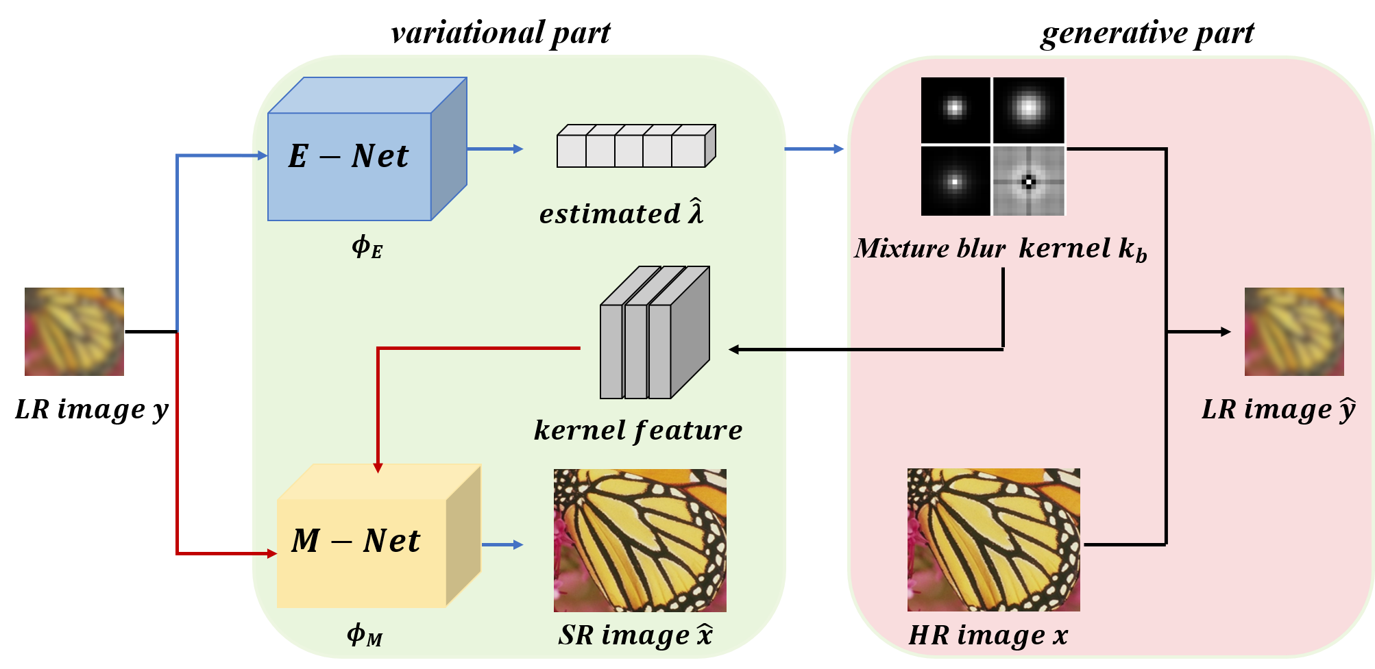
Fig. 1: The architecture of SREMN, consisting of an E-Net for blur kernel bandwidths and an M-Net for HR images.

3.1 Neural Modules

In E-step, the optimization of $q$ is required. Following the mixture kernel assumption in Eq. (2), we assume that $q$ is exponential with hyper-parameter $\hat{\boldsymbol{\lambda}}$ learned by the E-Net,

$$q(\mathbf{b}^{2})=\mathcal{E}(\mathbf{b}^{2};\hat{\boldsymbol{\lambda}}),~{}\hat{\boldsymbol{\lambda}}=f_{\boldsymbol{\phi}_{E}}(\mathbf{y})$$ (7)

where $f_{\boldsymbol{\phi}_{E}}(\cdot):\mathbf{y}\rightarrow\boldsymbol{\lambda}$ denotes a vector-valued function parameterized by $\boldsymbol{\phi}_{E}$ learned with the E-Net.

In M-step, the estimation of HR image $\mathbf{x}$ is achieved by

$$\hat{\mathbf{x}}=g_{\boldsymbol{\phi}_{M}}(\mathbf{y},\mathbf{k}_{\mathbf{b}})$$ (8)

where $g_{\boldsymbol{\phi}_{M}}(\cdot):\mathbf{y},\mathbf{k}_{\mathbf{b}}\rightarrow\mathbf{x}$ denotes a vector-valued function parameterized by $\boldsymbol{\phi}_{M}$ learned with the M-Net.

Therefore, the objective function of neural modules with respect to parameters $\boldsymbol{\phi}_{E}$ and $\boldsymbol{\phi}_{M}$ can be expressed as:

$$\quad\bar{\mathcal{F}}(\boldsymbol{\phi}_{E},\boldsymbol{\phi}_{M};\mathbf{y})$$ (9)

$$=\mathbb{E}_{\mathcal{E}(\mathbf{b}^{2};\hat{\lambda})}\big{[}\log p(\mathbf{y}|\mathbf{b}^{2},\hat{\mathbf{x}})\big{]}-\operatorname{D}_{KL}\big{(}\mathcal{E}(\hat{\lambda})\big{|}\big{|}\mathcal{E}(\lambda)\big{)}$$

where $\hat{\boldsymbol{\lambda}}=f_{\boldsymbol{\phi}_{E}}(\mathbf{y})$ and $\hat{\mathbf{x}}=g_{\boldsymbol{\phi}_{M}}(\mathbf{y},\mathbf{k}_{\mathbf{b}})$, $\mathbf{b}^{2}\sim\mathcal{E}(\mathbf{b}^{2};\hat{\boldsymbol{\lambda}})$.

Unfolded into an end-to-end learning network in Fig. 1, the optimization w.r.t. $\boldsymbol{\phi}_{E},\boldsymbol{\phi}_{M}$ can be expressed as follows,

$$\boldsymbol{\phi}_{E},\boldsymbol{\phi}_{M}=\arg\max_{\boldsymbol{\phi}_{E},\boldsymbol{\phi}_{M}}\bar{\mathcal{F}}(\boldsymbol{\phi}_{E},\boldsymbol{\phi}_{M};\mathbf{y})$$ (10)

3.2 Supervised and Semi-supervised Learning Schemes

Suppose we are given a labeled dataset $\mathcal{D}_{1}(\mathbf{X},\mathbf{Y})$ with $N$ i.i.d. sample pairs $\{\mathbf{x}_{i},\mathbf{y}_{i}\}_{i=1}^{N}$. Additionally we are given an unlabeled dataset $\mathcal{D}_{2}(\bar{\mathbf{Y}})$, with $M$ i.i.d. LR image samples $\{\mathbf{\bar{y}}_{j}\}_{j=1}^{M}$. Other than the common supervised learning on dataset $\mathcal{D}_{1}$, the proposed SREMN can utilize both data sets.

The overall loss function over the two datasets of the SREMN network is as follows:

$$\quad\mathcal{L}(\boldsymbol{\phi}_{E},\boldsymbol{\phi}_{M};\mathbf{X},\mathbf{Y},\mathbf{\bar{Y}})$$ (11)

$$=\alpha_{g}\cdot\mathcal{L}_{GEM}(\boldsymbol{\phi}_{E},\boldsymbol{\phi}_{M};\mathbf{Y},\mathbf{\bar{Y}})+\alpha_{r}\cdot\mathcal{L}_{REG}(\boldsymbol{\phi}_{E};\mathbf{X},\mathbf{Y}),$$

where $\alpha_{g},\alpha_{r}$ are fine-tuning weights to balance the effect of the GEM term and the regularization term over the given datasets. It can be seen that the amount of supervision can be safely adjusted by the number of samples in the two datasets.

The first term $\mathcal{L}_{GEM}(\boldsymbol{\phi}_{E},\boldsymbol{\phi}_{M};\mathbf{Y},\mathbf{\bar{Y}})$ is unsupervised, set to be the negative expectation of the GEM objective function over the given datasets, expressed as:

$$\mathcal{L}_{GEM}(\boldsymbol{\phi}_{E},\boldsymbol{\phi}_{M};\mathbf{Y},\mathbf{\bar{Y}})=-\mathbb{E}_{\mathbf{y}\sim\mathbf{Y},\mathbf{\bar{Y}}}\big{[}\bar{\mathcal{F}}(\boldsymbol{\phi}_{E},\boldsymbol{\phi}_{M};\mathbf{y})\big{]}.$$ (12)

The second term is a supervised one on $\mathcal{D}_{1}$ for regularization, expressed as:

$$\mathcal{L}_{SUP}(\boldsymbol{\phi}_{M};\mathbf{X},\mathbf{Y})=\mathbb{E}_{\mathbf{x},\mathbf{y}\sim\mathbf{X},\mathbf{Y}}\big{[}\|\mathbf{x}-g_{\boldsymbol{\phi}_{M}}(\mathbf{y})\|^{2}\big{]}.$$ (13)

Note that if there exist ground-truth kernels in the training set, i.e., $\mathcal{D}_{k}(\mathbf{K})=\{\mathbf{k}_{i}\}_{i=1}^{N}$ paired with $\mathcal{D}_{1}(\mathbf{X},\mathbf{Y})=\{\mathbf{x}_{i},\mathbf{y}_{i}\}_{i=1}^{N}$ is given, the supervised term can include the constraint on estimated kernels, expressed as:

$$\mathcal{L}_{SUP}(\boldsymbol{\phi}_{M};\mathbf{X},\mathbf{Y},\mathbf{K})= \mathbb{E}_{\mathbf{x},\mathbf{y}\sim\mathbf{X},\mathbf{Y}}\big{[}\|\mathbf{x}-g_{\boldsymbol{\phi}_{M}}(\mathbf{y})\|^{2}\big{]}$$ (14)

$$+\mathbb{E}_{\mathbf{k}\sim\mathbf{K}}\big{[}\|\mathbf{k}-\mathbf{k}_{\mathbf{b}}\|^{2}\big{]}.$$

4 Experiments

Table 1: Quantitative comparisons with SOTA SR methods. Best results are highlighted in red and blue respectively.

Types	Method	Scale $\times 2$		Scale $\times 4$
		PSNR	SSIM	PSNR	SSIM
Class $1$	Bicubic	28.73	0.8040	25.33	0.6795
	Bicubic kernel + ZSSR [15]	29.10	0.8215	25.61	0.6911
	EDSR [16]	29.17	0.8216	25.64	0.6928
	RCAN [14]	29.20	0.8223	25.66	0.6936
Class $2$	PDN [17] - $1$st in NTIRE’19 track4	/	/	26.34	0.7190
	WDSR [18]- $1$st in NTIRE’19 track2	/	/	21.55	0.6841
	WDSR [18]- $1$st in NTIRE’19 track3	/	/	21.54	0.7016
	WDSR [18]- $2$nd in NTIRE’19 track4	/	/	25.64	0.7144
	Ji et al. [19] - $1$st in NTIRE’20 track1	/	/	25.43	0.6907
Class $3$	Cornillere et al. [20]	29.46	0.8474	/	/
	Michaeli et al. [21] + SRMD [11]	25.51	0.8083	23.34	0.6530
	Michaeli et al. [21] + ZSSR [15]	29.37	0.8370	26.09	0.7138
	KernelGAN [8] + SRMD [11]	29.57	0.8564	25.71	0.7265
	KernelGAN [8] + USRNet [13]	/	/	20.06	0.5359
	KernelGAN [8] + ZSSR [15]	30.36	0.8669	26.81	0.7316
Class $4$	DAN [14]	32.56	0.8997	27.55	0.7582
	SREMN (OURS)	32.25	0.9370	27.74	0.8015

4.1 Experimental Setup

We adopt the experimental setting for training and testing first introduced in [8] and utilized in [14]. The training set includes $3450$ HR images from DIV2K [22] and Flick2K [23], with LR images synthesized by anisotropic Gaussian kernels. Benchmark dataset DIV2KRK is utilized as the testing set.

The Adam [24] optimizer is adopted for training. The learning rate is $0.0002$, and the decay of first and second momentum of gradients are $\beta_{1}=0.9$, $\beta_{2}=0.99$, respectively. All models are trained for $1000$ epochs with batch size $16$ on a single RTX1080Ti GPU.

We apply PSNR and SSIM metircs for image quality assessment, calculated on the Y-channel of transformed YCbCr space. We compare our method with competitors from four different classes four completeness, shown in Table 1.

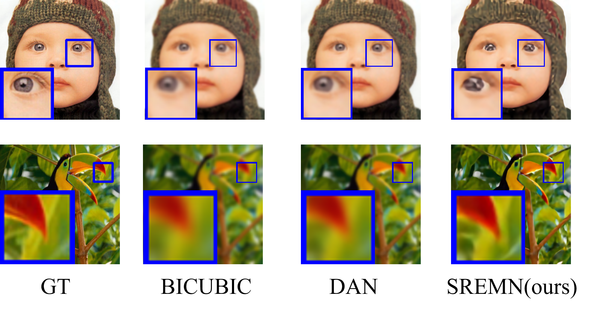
Fig. 2: Results of img $001$ and $002$ in Set5 (bandwidth 3.2).

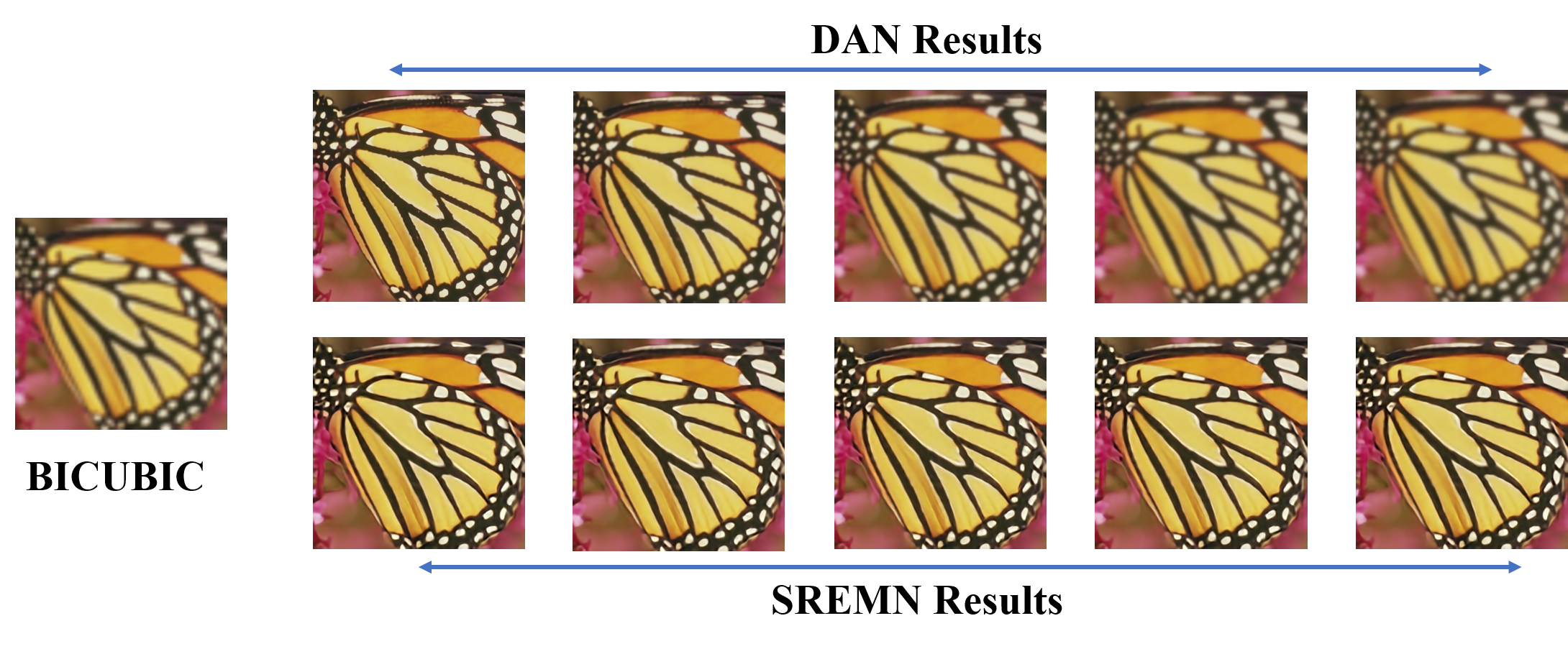
Fig. 3: Results of img $003$ in Set5 with the kernel bandwidths in $[1.8,2.2,2.6,3.0,3.2]$. It can be seen that the proposed SREMN is more robust over different settings.

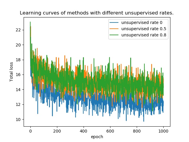
Fig. 4: Learning curves under different unsupervised rates. A higher rate results in a more challenging convergence of training.

4.2 Quantitative Results

Our method outperforms SOTA SR results of Blind SR with sequential steps while achieves similar results as DAN [14], a single step Blind SR method. Quantitative results are shown in Table 1. Our method gets nice ranks in both evaluation metrics, as it encourages diverse outputs with semantic variables and also has a well-defined objective function to regularize the generation. Though a little inferior to DAN in some cases, the proposed method shows some improvements in the qualitative perspective, as illustrated in Fig. 2. The inferiority may result from the following reasons: 1) We use a single RTX1080Ti GPU for training, while authors of DAN use distributed training with $8$ RTX2080Ti GPUs. 2) Our model is trained with the batch size of $16$, while DAN is trained with the batch size of $64$, enabled by distributed training. Therefore, the proposed method is considered to have comparable and more robust performance compared to DAN.

Table 2: Quantitative results of the proposed method with different unsupervised rates.

Methods	PSNR	SSIM	Time (H)
Semi-SREMN ($\eta=0$)	30.4240	0.9252	40.7
Semi-SREMN ($\eta=0.5$)	30.4901	0.9262	57.5
Semi-SREMN ($\eta=0.8$)	30.7218	0.9300	82.6

4.3 Semi-supervised Learning

Additional to $N$ samples of LR-HR pairs claimed above, we introduce $M$ LR samples without according HR samples to the training to see if our method can utilize such information. We define the unsupervised rate of the network learning as $\eta=M/(M+N)$, which increases with the amount of additional unlabeled data. We compare performances of the proposed approach under $3$ different supervision rates, i.e., $\eta=0,0.5,0.8$ for $M=0,N,4N$.

Quantitative results are shown in Table 2. It can be seen that models trained with higher supervision rate tend to have better results. This validate the proposed methodology that the potential of unlabeled data could be excavated by probabilistic modeling.

The learning curves of the proposed SREMN under different supervision rates are illustrated in Fig.4. It can be seen that the learning processes converges at around $600$ epochs, while the methods with higher supervision rates converge slower though with better ultimate performances, in accordance with intuition.

5 Conclusion

We propose a GEM framework for blind SISR (SREMN), which embeds the general image degradation model in a Bayesian model and enables efficient estimation of HR images. The proposed method leverages benefits from both model-based methods and learning-based methods, novel in conducting the blind SISR in a semi-supervised manner. Future work would be focused on a more flexible framework on image enhancing, integrating multiple related tasks.

References

- [1] W. Siu and K.-W. Hung, “Review of image interpolation and super-resolution,” Proceedings of The 2012 Asia Pacific Signal and Information Processing Association Annual Summit and Conference, pp. 1–10, 2012.
- [2] D. Dengxin, W. Yujian, C. Yuhua, and V. G. Luc, “Is image super-resolution helpful for other vision tasks?” in 2016 IEEE Winter Conference on Applications of Computer Vision (WACV), 2016, pp. 1–9.
- [3] M. Elad and A. Feuer, “Restoration of a single superresolution image from several blurred, noisy, and undersampled measured images,” IEEE transactions on image processing : a publication of the IEEE Signal Processing Society, vol. 6 12, pp. 1646–58, 1997.
- [4] C. Liu and D. Sun, “On bayesian adaptive video super resolution,” IEEE Transactions on Pattern Analysis and Machine Intelligence, vol. 36, pp. 346–360, 2014.
- [5] C. Dong, C. C. Loy, K. He, and X. Tang, “Learning a deep convolutional network for image super-resolution,” in ECCV, 2014.
- [6] Y. Zhang, Y. Tian, Y. Kong, B. Zhong, and Y. Fu, “Residual dense network for image super-resolution,” 2018 IEEE/CVF Conference on Computer Vision and Pattern Recognition, pp. 2472–2481, 2018.
- [7] X. Wang, K. Yu, S. Wu, J. Gu, Y.-H. Liu, C. Dong, C. C. Loy, Y. Qiao, and X. Tang, “Esrgan: Enhanced super-resolution generative adversarial networks,” in ECCV Workshops, 2018.
- [8] S. Bell-Kligler, A. Shocher, and M. Irani, “Blind super-resolution kernel estimation using an internal-gan,” in NeurIPS, 2019.
- [9] A. Bulat, J. Yang, and G. Tzimiropoulos, “To learn image super-resolution, use a gan to learn how to do image degradation first,” in ECCV, 2018.
- [10] J. Gu, H. Lu, W. Zuo, and C. Dong, “Blind super-resolution with iterative kernel correction,” 2019 IEEE/CVF Conference on Computer Vision and Pattern Recognition (CVPR), pp. 1604–1613, 2019.
- [11] K. Zhang, W. Zuo, and L. Zhang, “Learning a single convolutional super-resolution network for multiple degradations,” 2018 IEEE/CVF Conference on Computer Vision and Pattern Recognition, pp. 3262–3271, 2018.
- [12] ——, “Deep plug-and-play super-resolution for arbitrary blur kernels,” 2019 IEEE/CVF Conference on Computer Vision and Pattern Recognition (CVPR), pp. 1671–1681, 2019.
- [13] K. Zhang, L. Gool, and R. Timofte, “Deep unfolding network for image super-resolution,” 2020 IEEE/CVF Conference on Computer Vision and Pattern Recognition (CVPR), pp. 3214–3223, 2020.
- [14] Z. Luo, Y. Huang, S. Li, L. Wang, and T. Tan, “Unfolding the alternating optimization for blind super resolution,” ArXiv, vol. abs/2010.02631, 2020.
- [15] A. Shocher, N. Cohen, and M. Irani, “”zero-shot” super-resolution using deep internal learning,” in CVPR, 2018.
- [16] B. Lim, S. Son, H. Kim, S. Nah, and K. M. Lee, “Enhanced deep residual networks for single image super-resolution,” 2017 IEEE Conference on Computer Vision and Pattern Recognition Workshops (CVPRW), pp. 1132–1140, 2017.
- [17] J. Ma, X. Wang, and J. Jiang, “Image superresolution via dense discriminative network,” IEEE Transactions on Industrial Electronics, vol. 67, pp. 5687–5695, 2020.
- [18] J. Yu, Y. Fan, J. Yang, N. Xu, Z. Wang, X. Wang, and T. Huang, “Wide activation for efficient and accurate image super-resolution,” ArXiv, vol. abs/1808.08718, 2018.
- [19] X. Ji, Y. Cao, Y. Tai, C. Wang, J. Li, and F. Huang, “Real-world super-resolution via kernel estimation and noise injection,” 2020 IEEE/CVF Conference on Computer Vision and Pattern Recognition Workshops (CVPRW), pp. 1914–1923, 2020.
- [20] V. Cornillère, A. Djelouah, Y. Wang, O. Sorkine-Hornung, and C. Schroers, “Blind image super-resolution with spatially variant degradations,” ACM Transactions on Graphics (TOG), vol. 38, pp. 1 – 13, 2019.
- [21] T. Michaeli and M. Irani, “Nonparametric blind super-resolution,” 2013 IEEE International Conference on Computer Vision, pp. 945–952, 2013.
- [22] E. Agustsson and R. Timofte, “Ntire 2017 challenge on single image super-resolution: Dataset and study,” 2017 IEEE Conference on Computer Vision and Pattern Recognition Workshops (CVPRW), pp. 1122–1131, 2017.
- [23] R. T. et al., “Ntire 2017 challenge on single image super-resolution: Methods and results,” in 2017 IEEE Conference on Computer Vision and Pattern Recognition Workshops (CVPRW), 2017, pp. 1110–1121.
- [24] D. P. Kingma and J. Ba, “Adam: A method for stochastic optimization,” CoRR, vol. abs/1412.6980, 2015.