Continual Learning on Dynamic Graphs via Parameter Isolation

Abstract.

Many real-world graph learning tasks require handling dynamic graphs where new nodes and edges emerge. Dynamic graph learning methods commonly suffer from the catastrophic forgetting problem, where knowledge learned for previous graphs is overwritten by updates for new graphs. To alleviate the problem, continual graph learning methods are proposed. However, existing continual graph learning methods aim to learn new patterns and maintain old ones with the same set of parameters of fixed size, and thus face a fundamental tradeoff between both goals. In this paper, we propose Parameter Isolation GNN (PI-GNN) for continual learning on dynamic graphs that circumvents the tradeoff via parameter isolation and expansion. Our motivation lies in that different parameters contribute to learning different graph patterns. Based on the idea, we expand model parameters to continually learn emerging graph patterns. Meanwhile, to effectively preserve knowledge for unaffected patterns, we find parameters that correspond to them via optimization and freeze them to prevent them from being rewritten. Experiments on eight real-world datasets corroborate the effectiveness of PI-GNN compared to state-of-the-art baselines.

1. Introduction

Graphs are ubiquitous around our life describing a wide range of relational data. Substantial endeavors have been made to learn desirable graph representations to facilitate graph data analysis (Grover and Leskovec, 2016; Perozzi et al., 2014; Tang et al., 2015; Kipf and Welling, 2016; Hamilton et al., 2017; Jin et al., 2022a, b; Veličković et al., 2017; Huang et al., 2022; Yang et al., 2022; Guo et al., 2022a; Zhang et al., 2023; Guo et al., 2022b). Graph Neural Networks (GNNs) (Zhao et al., 2022; Zhang et al., 2022; Pang et al., 2022; Li et al., 2022; Ma et al., 2022; Xu et al., 2018; Wu et al., 2019; Guo et al., 2023; Klicpera et al., 2020b; He et al., 2020; Klicpera et al., 2020a) take advantage of deep learning to fuse node features and topological structures, achieving state-of-the-art performance in a myriad of applications.

Conventional GNNs are specifically designed for static graphs, while real-life graphs are inherently dynamic. For example, edges are added or removed in social networks when users decide to follow or unfollow others. Various graph learning approaches are proposed to tackle the challenge of mutable topology by encoding new patterns into the parameter set, e.g., incorporating the time dimension. Nevertheless, these methods primarily focus on capturing new emerging topological patterns, which might overwhelm the previously learned knowledge, leading to a phenomenon called the catastrophic forgetting (McCloskey and Cohen, 1989; Ratcliff, 1990; French, 1999; Jin et al., 2023; Shi et al., 2021; Zhang and Kim, 2023). To address catastrophic forgetting in dynamic graphs, continual graph learning methods are proposed (Wang et al., 2020b; Zhou and Cao, 2021) to learn emerging graph patterns while maintaining old ones in previous snapshots.

Existing continual graph learning methods generally apply techniques such as data replay (Shin et al., 2017; Lopez-Paz and Ranzato, 2017; Rebuffi et al., 2017; Rolnick et al., 2018; Yoon et al., 2017) and regularizations (Kirkpatrick et al., 2017; Zenke et al., 2017; Li and Hoiem, 2017; Aljundi et al., 2018; Ramesh and Chaudhari, 2021; Ke et al., 2020; Hung et al., 2019) to alleviate catastrophic forgetting in dynamic graphs. However, these approaches are still plagued by seeking a desirable equilibrium between capturing new patterns and maintaining old ones due to two reasons.

• On one hand, existing methods use the same parameter set to preserve both old and new patterns in dynamic graphs. Consequently, new patterns are learned at the inevitable expense of overwriting the parameters encoding old patterns, leading to the potential forgetting of previous knowledge.

• On the other hand, existing methods use parameters with fixed size throughout the dynamic graph. As parameters with a fixed size may only capture a finite number of graph patterns, compromises have to be made between learning new graph patterns and maintaining old ones.

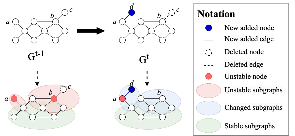
Figure 1. Illustration of stable, unstable, and changed subgraphs with $k=1$. At snapshot $t$, a new node $d$ connects to $a$ and node $c$ is deleted. Thus, the neighborhoods of $a,b$ are unstable subgraphs at snapshot $t-1$ (red shades). Unstable subgraphs will become changed ones after adding and deleting nodes and edges at snapshot $t$ (blue shades). The green shades denote stable subgraphs.

Moreover, such shared and fixed parameter set might be potentially not suitable in dynamic graph settings. On the one hand, graph evolution can be quite flexible. As shown in Figure 1, nodes anywhere can be added or deleted, resulting in dramatic changes in each snapshot. On the other hand, unlike non-graph data, e.g., images, where no coupling relationship exists between the data, nodes in the graph can be deeply coupled. As shown in Figure 1, newly added/dropped nodes will affect the states of their neighborhood nodes, leading to the cascaded changes of node states. Therefore, how to perform continual learning in such dramatically and cascadedly changing situation is the unique challenge for continual graph learning. As the emerging patterns in dynamic graphs can be informative, the shared and fixed parameter set will be affected significantly that corrupts old patterns, which inspires us to utilize extra parameters to capture these informative patterns.

Parameter isolation, a continual learning method with the intuition that different types of patterns in terms of temporal are captured by different sets of parameters (Rusu et al., 2016), naturally fits the unique challenge of continual graph learning. Thus, to break the tradeoff between learning new patterns and maintaining old ones in dynamic graphs, we propose to utilize parameter isolation to apply separate and expanding parameters to capture the emerging patterns without sacrificing old patterns of the stable graph.

In particular, applying parameter isolation in continual graph learning is challenging. First of all, existing parameter isolation approaches (Rusu et al., 2016; Rosenfeld and Tsotsos, 2018; Yoon et al., 2017; Fernando et al., 2017) are for data in Euclidean space, e.g., images, which cannot capture the influence of cascading changes in dynamic graphs well. Second, during the graph evolution process, parameter isolation methods continually expand the model scale and suffer the dramatically increased parameters (Rusu et al., 2016). Last but not least, as existing methods cannot provide theoretical guarantees to ensure the ability of the parameter isolation process, unstable and inconsistent training may occur due to the dynamic data properties.

To address these issues, we propose a novel Parameter Isolation GNN (PI-GNN) model for continual learning on dynamic graphs. To adapt to the unique challenges of continual graph learning, at the data level, the whole graph pattern is divided into stable and unstable parts to model the cascading influences among nodes. At the model level, PI-GNN is designed to consist of two consecutive stages: the knowledge rectification stage and the parameter isolation stage. As the foundation for parameter isolation, the knowledge rectification stage filters out the impact of patterns affected by changed nodes and edges. We fine-tune the model to exclude such impact and get stable parameters that maintain performance over existing stable graph patterns. In the parameter isolation stage, we keep the stable parameters frozen, while expanding the model with new parameters, such that new graph patterns are accommodated without compromising stable ones. To prevent the model from excessive expansion, we use model distillation to compress the model while maintaining its performance. Finally, we provide theoretical analysis specifically from the perspective of graph data to justify the ability of our method. We theoretically show that the parameter isolation stage optimizes a tight upper bound of the retraining loss on the entire graph. Extensive experiments are conducted on eight real-world datasets, where PI-GNN outperforms state-of-the-art baselines for continual learning on dynamic graphs. We release our code at https://github.com/Jerry2398/PI-GNN.

Our contributions are summarized as follows:

• We propose PI-GNN, a continual learning method on dynamic graphs based on parameter isolation. By isolating stable parameters and learning new patterns with parameter expansion, PI-GNN not only captures emerging patterns but also suffers less from catastrophic forgetting.

• We theoretically prove that PI-GNN optimizes a tight upper bound of the retraining loss on the entire graph.

• We conduct extensive evaluations on eight real-world datasets, where PI-GNN achieves state-of-the-art on dynamic graphs.

2. Preliminaries

In this section, we first present preliminaries on dynamic graphs, and then formulate the problem definition.

Definition 1 (Dynamic Graph). A graph at snapshot $t$ is denoted as $G^{t}=(V^{t},\mathbf{A}^{t},\mathbf{X}^{t})$, where $V^{t}$ is the set of nodes, $\mathbf{A}^{t}$ is the adjacency matrix, and $\mathbf{X}^{t}$ are node features. A dynamic graph is denoted as $\mathcal{G}=(G^{1},...,G^{T-1},G^{T})$, with $T$ the number of snapshots.

Definition 2 (Graph Neural Networks (GNNs)). We denote a $k$-layer GNN parameterized by $\theta^{t}$ as $f_{\theta^{t}}$, the representations of node $v$ in layer $l$ as $\mathbf{h}_{v}^{(l)}$ and $\mathbf{h}_{v}^{(0)}=\mathbf{X}_{v}$. The representations of node $v$ is updated by message passing as follows:

(1) $$\mathbf{h}_{v}^{(l+1)}=\mathrm{COMB}\left(\mathrm{AGG}\left(\mathbf{h}_{u}^{(l)},\forall u\in N(v)\right),\mathbf{h}_{v}^{(l)}\right),$$

where $N(v)$ is the neighborhood of node $v$, AGG and COMB denote GNNs’ message passing and aggregation mechanisms, respectively.

With $y_{v}$ as the label of $v$, the loss of node classification is:

(2) $$L\left(f_{\theta^{t}}\left(G^{t}\right)\right)=\sum_{v\in V^{t}}\mathrm{CrossEnt}\left(\mathrm{softmax}\left(\mathbf{h}_{v}^{(k)}\right),y_{v}\right).$$

In dynamic graphs, some subgraphs at snapshot $t$ will be affected by new or deleted graph data at $t+1$ (Pareja et al., 2020). Based on this motivation, we decompose the graph into stable and unstable subgraphs:

• Unstable subgraphs $G_{unstable}^{t-1}$ are defined as the $k$-hop ego-subgraphs at snapshot $t-1$ that centered with nodes directly connected to emerging/deleted nodes or edges at snapshot $t$.

• Stable subgraphs $G_{stable}^{t-1}$ are defined as the $k$-hop ego-subgraphs whose center nodes are outside the $k$-hop ranges of nodes connecting to emerging/deleted nodes or edges at snapshot $t$, i.e. $G_{stable}^{t-1}=G^{t-1}-G_{unstable}^{t-1}$.

• Changed subgraphs $\Delta G^{t}$ evolve from $G_{unstable}^{t-1}$ after new nodes and edges are added or deleted at snapshot $t$.

Note that $G_{stable}$ and $G_{unstable}$ refers to ego-networks while the operation conducted on $G_{stable}$ and $G_{unstable}$ only involves their central nodes. As the node is either stable or unstable, $G_{stable}=G-G_{unstable}$ will hold. Although the ego-networks might be overlapping, this won’t affect the above equation.

Based on these definitions, we have

(3) $$L\left(f_{\theta^{t-1}}\left(G^{t-1}\right)\right)$$

$$=L\left(f_{\theta^{t-1}}\left(G_{stable}^{t-1}\right)\right)+L\left(f_{\theta^{t-1}}\left(G_{unstable}^{t-1}\right)\right),$$

Note that the loss of node classification is computed in units of nodes. Therefore, the loss function in r.h.s of Eqn. 3 can be directly added up so that Eqn. 3 will hold.

As $G_{stable}^{t-1}$ will remain unchanged at snapshot $t$ while $G_{unstable}^{t-1}$ will evolve into $\Delta G^{t}$, we have

(4) $$L\left(f_{\theta^{t}}\left(G^{t}\right)\right)=L\left(f_{\theta^{t}}\left(G_{stable}^{t-1}\right)\right)+L\left(f_{\theta^{t}}\left(\Delta G^{t}\right)\right)$$

We finally define the problem of continual learning for GNNs.

Definition 3 (Continual Learning for GNNs). The goal of continual learning for GNNs is to learn a series of parameters $\theta=(\theta^{1},\theta^{2},...,\theta^{T})$ given a dynamic graph $\mathcal{G}=(G^{1},G^{2},...,G^{T})$, where $f_{\theta^{t}}$ perform well on $G^{i\leq t}$, i.e. graphs from all previous snapshots.

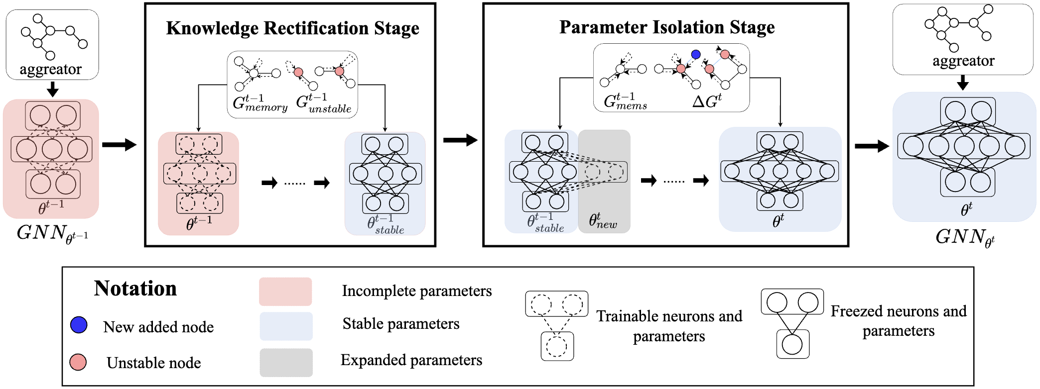
Figure 2. An overview of PI-GNN. There are two consecutive stages in PI-GNN: the knowledge rectification stage and the parameter isolation stage. The knowledge rectification stage is used to obtain stable model parameters, while the parameter isolation stage is used to learn new patterns without compromising existing stable patterns.

3. Methodology

In this section, we introduce the details of PI-GNN, as shown in Figure 2. PI-GNN contains two stages. In the knowledge rectification stage, the GNN model is trained to learn stable paramters to capture topological structure within the stable subgraphs. In the parameter isolation stage, the GNN model is further expanded to capture the new patterns within the unstable subgraphs while the stable parameters are fixed from being rewritten. Theoretical analysis are presented to justify the capacity of both stages to comprehensively capture new and stable patterns at each snapshot.

3.1. Knowledge Rectification

The knowledge rectification stage is used to update the model to obtain parameters that capture the topological patterns of stable subgraphs. The design philosophy behind the knowledge rectification is that $\theta^{t-1}$ may not be the optimal initialization for snapshot $t$ because they may encode irrelevant data patterns. Specifically, as nodes are connected with each other, new nodes and edges at snapshot $t$ will have an influence on existing nodes at $t-1$, which constitute unstable subgraphs $G_{unstable}^{t-1}$ that change at snapshot $t$. Thus, only the stable subgraphs $G_{stable}^{t-1}$ should be shared between $G^{t-1}$ and $G^{t}$, and consequently, we need to initialize $\theta^{t}$ that best fits $G_{stable}^{t-1}$ instead of $G^{t-1}$. We achieve this goal by the following optimization. From Eqn. 3, we have:

(5) $$\min_{\theta^{t-1}}\;L\left(f_{\theta^{t-1}}\left(G_{stable}^{t-1}\right)\right)$$

$$\Leftrightarrow \min_{\theta^{t-1}}\;L\left(f_{\theta^{t-1}}\left(G^{t-1}\right)\right)-L\left(f_{\theta^{t-1}}\left(G_{unstable}^{t-1}\right)\right).$$

By optimizing the model via Eqn. 5, we get parameters encoding $G_{stable}^{t-1}$ which will remain unchanged at snapshot $t$. We denote them as stable parameters. In Eqn. 5, $G_{unstable}^{t-1}$ can be easily obtained from $\Delta G^{t}$ through its definition. However, it is time-consuming to re-compute $L(f_{\theta^{t-1}}(G^{t-1}))$. We thus sample and store some nodes from $G^{t-1}$ and use their $k$-hop neighborhoods (referred to as $G_{memory}^{t-1}$) to estimate $L(f_{\theta^{t-1}}(G^{t-1}))$. We adopt uniform sampling to ensure unbiasedness. Therefore, in practice, the following optimization problem is solved for the knowledge rectification stage,

(6) $$\theta^{t-1}_{stable}=\arg\min_{\theta^{t-1}} L(f_{\theta^{t-1}}(G_{memory}^{t-1}))$$

$$- \beta L(f_{\theta^{t-1}}(G_{unstable}^{t-1})),$$

where $\theta_{stable}^{t-1}$ are the stable parameters, $\beta$ is a factor to handle the size imbalance problem caused by sampling $G_{memory}^{t-1}$.

3.2. Parameter Isolation

After obtaining the stable parameters, we propose a parameter isolation algorithm for GNNs to learn new patterns incrementally without compromising the stable patterns.

3.2.1. Algorithm

The key idea of parameter isolation is that different parameters can learn different patterns, and that instead of modifying existing parameters, we isolate and add new parameters to learn new patterns. Specifically, we show the parameter isolation algorithm at snapshot $t$ in Figure 3, which can be divided as follows:

1. Expand: We expand parameters for hidden layers $\theta_{stable}^{t-1}$ to $\theta^{t}=\theta_{stable}^{t-1}\oplus\theta_{new}^{t}$, so as to increase the model capacity to learn new patterns.

2. Freeze: We freeze $\theta_{stable}^{t-1}$ to prevent them from being rewritten. Considering that old patterns may benefit learning new graph patterns, $\theta_{stable}^{t-1}$ are used to compute the loss during the forward pass but will not be updated.

3. Update: We update $\theta_{new}^{t}$ on the graph $G^{t}$. For efficient training, $\theta_{new}^{t}$ are updated only on $\Delta G^{t}$ and $G^{t-1}_{memory}$. Formally, we optimize the following objective

   (7) $$\min_{\theta_{new}^{t}} L\left(f_{\theta^{t-1}_{stable}}\left(\Delta G^{t}\right)+f_{\theta_{new}^{t}}\left(\Delta G^{t}\right)\right)$$

   $$+\lambda\,L(f_{\theta_{new}^{t}}(G_{memory}^{t-1})),$$

   where $G_{memory}^{t-1}$ is the stable subset of $G_{memory}^{t-1}$, and $\lambda$ is similar to $\beta$ in Eqn. 6 that handles the size imbalance problem caused by sampling $G_{memory}^{t-1}$.

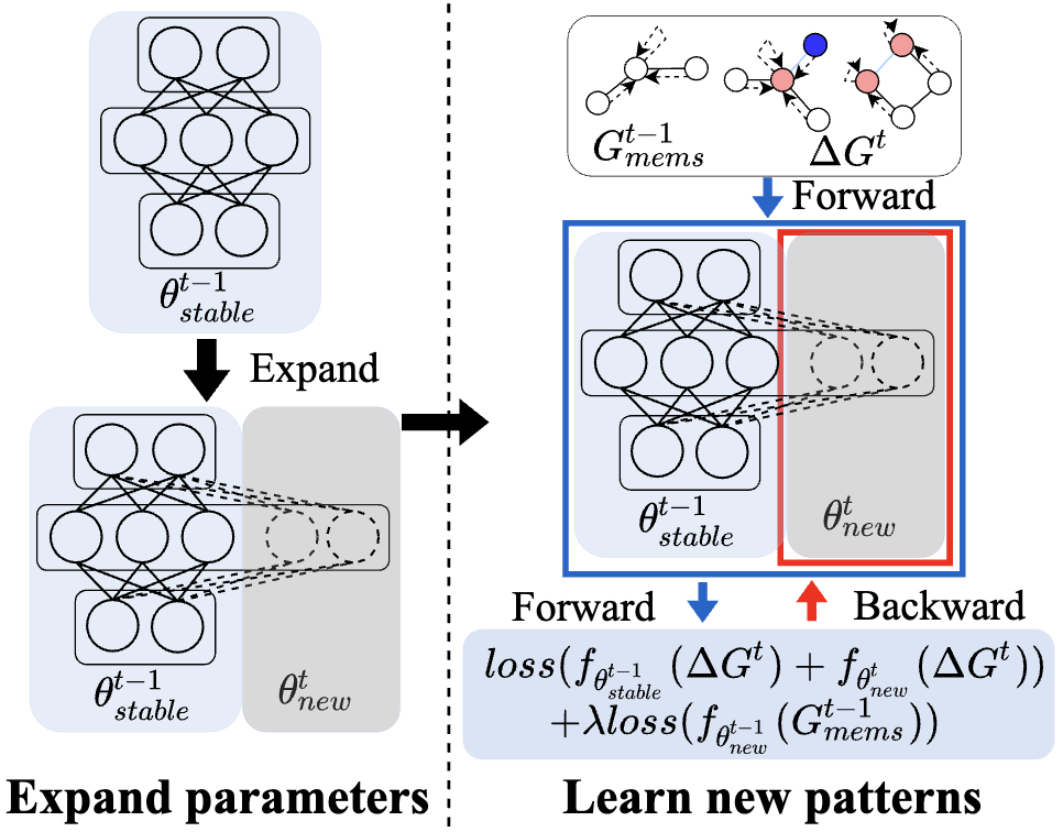
Figure 3. Illustration of parameter isolation stage.

3.3. Theoretical Analysis

We conduct theoretical analysis to guarantee the correctness of the proposed parameter isolation algorithm on dynamic graphs. We first present the main theorem as follows:

Theorem 3.1.

(8) $$L\left(f_{\theta^{t}}\left(G^{t}\right)\right) \leq L\left(f_{\theta^{t-1}_{stable}}\left(\Delta G^{t}\right)+f_{\theta_{new}^{t}}\left(\Delta G^{t}\right)\right)$$

$$+\frac{1}{2}L\left(f_{\theta_{stable}^{t-1}}\left(G_{stable}^{t-1}\right)\right)+\frac{1}{2}L\left(f_{\theta_{new}^{t}}\left(G_{stable}^{t-1}\right)\right)$$

and equality holds when $f_{\theta_{new}^{t}}(G_{stable}^{t-1})=f_{\theta_{stable}^{t-1}}(G_{stable}^{t-1})$.

The implication of Theorem 3.1 is that by splitting $\theta^{t}=\theta_{new}^{t}\oplus\theta^{t-1}_{stable}$ and $G^{t}=G^{t-1}_{stable}\cup\Delta G^{t}$, we actually optimize a tight upper bound (R.H.S. of Eqn. 8) of the retraining loss $L(f_{\theta^{t}}(G^{t}))$ at snapshot $t$. To prove the theorem, we first show a lemma whose proof can be found in the Appendix A.1.

Lemma 3.2.

$2L(f_{\theta_{1}}(G)+f_{\theta_{2}}(G))\leq L(f_{\theta_{1}}(G))+L(f_{\theta_{2}}(G))$ where the equality holds if $f_{\theta_{1}}(G)=f_{\theta_{2}}(G)$.

Lemma 3.2 essentially follows from the convexity of the cross entropy loss. We then provide proof to Theorem 3.1.

Proof.

From Eqn. 4, $\theta^{t}=\theta_{stable}^{t-1}\oplus\theta_{new}^{t}$ and Lemma 3.2,

(9) $$\;L\left(f_{\theta^{t}}\left(G^{t}\right)\right)$$

$$= \;L\left(f_{\theta^{t}}\left(\Delta G^{t}\right)\right)+L\left(f_{\theta^{t}}\left(G^{t-1}_{stable}\right)\right)$$

$$= \;L\left(f_{\theta^{t-1}_{stable}}\left(\Delta G^{t}\right)+f_{\theta_{new}^{t}}\left(\Delta G^{t}\right)\right)$$

$$+L\left(f_{\theta^{t-1}_{stable}}\left(G^{t-1}_{stable}\right)+f_{\theta_{new}^{t}}\left(G^{t-1}_{stable}\right)\right)$$

$$\leq \;L\left(f_{\theta^{t-1}_{stable}}\left(\Delta G^{t}\right)+f_{\theta_{new}^{t}}\left(\Delta G^{t}\right)\right)$$

$$+\frac{1}{2}L\left(f_{\theta^{t-1}_{stable}}\left(G^{t-1}_{stable}\right)\right)+\frac{1}{2}L\left(f_{\theta_{new}^{t}}\left(G^{t-1}_{stable}\right)\right).$$

From Lemma 3.2, equality holds if $f_{\theta_{new}^{t}}(G_{stable}^{t-1})=f_{\theta_{stable}^{t-1}}(G_{stable}^{t-1})$. Therefore we prove Theorem 3.1. ∎

3.3.1. Practical Implementation

We discuss how to optimize the upper bound (R.H.S. of Eqn. 8) in practice. The second term
$L(f_{\theta^{t-1}_{stable}}(G^{t-1}_{stable}))$ has been optimized in Eqn. 6 and $\theta_{stable}^{t-1}$ are fixed. Therefore, we only need to optimize the first and third terms.

For the first term of the upper bound, as $\theta^{t-1}_{stable}$ are frozen to preserve the stable parameters, we only optimize on $\theta_{new}^{t}$. Thus, we optimize the first term as

(10) $$\min_{\theta_{new}^{t}}\;L\left(f_{\theta^{t-1}_{stable}}\left(\Delta G^{t}\right)+f_{\theta_{new}^{t}}\left(\Delta G^{t}\right)\right).$$

For the third term, we use $G_{memory}^{t-1}$ to estimate $G^{t-1}_{stable}$. Thus, the third term can be approximately optimized as

(11) $$\min_{\theta_{new}^{t}}\lambda L(f_{\theta_{new}^{t}}(G_{memory}^{t-1})),$$

where $\lambda$ is a balance factor to compensate for the size difference between $G_{memory}^{t-1}$ and $G_{stable}^{t-1}$. Combining Eqn. 10 and Eqn. 11, we obtain the final optimization problem in Eqn. 7.

3.3.2. Bound Analysis

From Lemma 3.2, the equality holds if
$f_{\theta_{new}^{t}}(G_{stable}^{t-1})=f_{\theta_{stable}^{t-1}}(G_{stable}^{t-1})$. As ${\theta_{stable}^{t-1}}$ has been optimized in the knowledge rectification stage, $\theta_{stable}^{t-1}$ minimizes $L(f_{\theta^{t-1}}(G_{stable}^{t-1}))$. In addition, as we minimize $L(f_{\theta_{new}^{t}}(G_{memory}^{t-1}))$ and $G_{memory}^{t-1}$ are sampled from $G_{stable}^{t-1}$, we also push $\theta_{new}^{t}$ close to the minimizer $\theta_{stable}^{t-1}$. Thus, the tightness of the bound in Eqn. 7 can be ensured.

3.4. Discussions

Model Compression. Parameter isolation suffers the dramatically increased parameters for large $T$ (Rusu et al., 2016). We adopt model distillation (Hinton et al., 2015) to solve this problem, where we use the original model as the teacher model and another model with fewer hidden units as the student model (i.e., the compressed model). We minimize the cross entropy between the outputs of the teacher and student models. Specifically, we use $G_{memory}$ as the stable data and $\Delta{G}$ as the new data, altogether severs as our training data for distillation. This is in line with our settings, as these data can be obtained in the knowledge rectification stage, and no additional knowledge is introduced.

Another issue is that if graph patterns disappear significantly due to node/edge deletions, an overly expanded model may face the overfitting problem. This can also be solved by model distillation. When too many nodes or edges are deleted in dynamic graphs compared to the previous snapshot, we can distill the model to get a smaller model at this snapshot to avoid the overfitting problem.

In our experiments, we compress our model on graph $G^{T}$ after the last snapshot. As there is no end on the snapshots in real-world applications, the model can be compressed regularly at any time and this barely affect the performance.

Extension to Other Tasks. Throughout the paper, we mainly focus on node classification tasks as in (Wang et al., 2020b; Zhou and Cao, 2021). However, the theory stated in Theorem 3.1 holds for other tasks as long as the loss function is convex. Parameter isolation for other tasks (e.g. link prediction) may require minor design modifications (e.g. graph decomposition, choice of samples), and thus we leave them as future work.

4. Experiments

	Nodes	Edges	Attributes	# Tasks
Cora	2,708	5,429	1,433	14
Citeseer	3,327	4,732	3,703	12
Amazon Photo	7,650	119,043	745	16
Amazon Computer	13,752	491,722	767	18
Elliptic	31,448	23,230	166	9
DBLP-S	20,000	75,706	128	26
Arxiv-S	40,726	88,691	128	13
Paper100M-S	49,459	108,710	128	11

Table 1. Statistics of the eight datasets.

In this section, we present the empirical evaluations of PI-GNN on eight real-world datasets ranging from citation networks (McCallum et al., 2000; Sen et al., 2008; Tang et al., 2008; Wang et al., 2020a) to bitcoin transaction networks (Weber et al., 2019) and e-commercial networks (Shchur et al., 2018).

4.1. Experimental Setup

4.1.1. Datasets

We conduct experiments on eight real-world graph datasets with diverse application scenarios: Cora (McCallum et al., 2000), Citeseer (Sen et al., 2008), Amazon Photo (Shchur et al., 2018), Amazon Computer (Shchur et al., 2018), Elliptic (Weber et al., 2019), DBLP-S (Tang et al., 2008), Arxiv-S, and Paper100M-S (Wang et al., 2020a). Among them, Elliptic, DBLP-S, Arxiv-S, and Paper100M-S are streaming graphs. We sample from their full data and we split them into tasks according to the timestamps. For Arxiv-S, we choose a subgraph with 5 classes whose nodes number have top variations from year 2010 to year 2018 from Arxiv full data. We split it into tasks according to the timestamps. For DBLP-S, we randomly choose 20000 nodes with 9 classes and 75706 edges from DBLP full data, we split it into tasks according to the timestamps. For Paper100M-S, we randomly choose 12 classes from year 2009 to year 2019 from Paper100M full data and we split it into tasks according to the timestamps. Alternatively, as Cora, Citeseer, Amazon Photo and Amazon Computer are static graphs, we manually transform them into streaming graphs according to the task-incremental setting, where we add one class every two tasks.

For each dataset, we split 60% of nodes in $G^{T}$ for training, 20% for validation and 20% for test. The train/val/test split is consistent across all snapshots. Dataset statistics are shown in Table 1.

4.1.2. Baselines

We compare PI-GNN with the following baselines.

• Retrain: We retrain a GNN on $G^{t}$ at each snapshot. As all patterns are learned for each snapshot, it can be seen as an upper bound for all continual learning methods.

• Pretrain We use a GNN trained on $G^{1}$ for all snapshots.

• OnlineGNN: We train a GNN on $G^{1}$ and fine tune it on the changed subgraphs $\Delta G^{t}$ at each snapshot $t$.

• Dynamic baselines: We compare PI-GNN with the following methods on general dynamic graph learning: EvolveGCN (Pareja et al., 2020), DyGNN (Ma et al., 2020), and DNE (Du et al., 2018).

• Continual baselines: We compare PI-GNN with the following methods on continual graph learning: ContinualGNN  (Wang et al., 2020b), DiCGRL  (Kou et al., 2020), and TWP  (Liu et al., 2021).

4.1.3. Hyperparameter Settings

GraphSAGE with $k=2$ layers is used as the backbone of Retrain, OnlineGNN, Pretrain and PI-GNN. We initialize 12 units for each hidden layer and expand 12 units at each snapshot. We set $\lambda=0.1,\beta=0.01$. We sample 128 nodes for Arxiv-S as $G_{memory}$ and 256 nodes for other datasets. After training, we distill PI-GNN to a smaller model with 32 hidden units. We apply grid search to find the optimal hyper-parameters for each model. For fairness, all the baselines use backbone models with the final (i.e. largest) capacity of PI-GNN before distillation to eliminate the influence of different parameter size of models.

		Lower bound	Incremental	Dynamic			Continual			Upper bound	Ours
Dataset	Metric	Pretrain	OnlineGNN	EvolveGCN	DyGNN	DNE	ContinualGNN	DiCGRL	TWP	Retrain	PI-GNN	Distilled PI-GNN
Arxiv-S	PM	45.99$\pm$1.99%.	72.69$\pm$1.31%	74.08$\pm$0.35%	61.13$\pm$2.97%	39.13$\pm$5.97%	75.36$\pm$0.21%	67.93$\pm$0.97%	73.91$\pm$0.14%	81.86$\pm$0.28%	77.02$\pm$0.53%	76.50$\pm$0.38%
	FM	0$\pm$0%.	-8.57$\pm$1.77%	-5.55$\pm$0.33%	-6.98$\pm$2.18%	-16.98$\pm$2.18%	-2.17$\pm$0.07%	-2.91$\pm$0.44%	-2.12$\pm$0.29%	-0.12$\pm$0.06%	-1.22$\pm$0.03%	-1.71$\pm$0.20%
DBLP-S	PM	43.17$\pm$1.45%	63.52$\pm$1.07%	61.52$\pm$1.34%	54.32$\pm$2.75%	32.44$\pm$6.17%	62.67$\pm$0.06%	57.09$\pm$4.13%	55.82$\pm$4.73%	64.77$\pm$1.01%	64.76$\pm$0.19%	63.49$\pm$0.45%
	FM	0$\pm$0%	-5.04$\pm$0.46%	-4.91$\pm$0.23%	-8.62$\pm$2.33%	-15.62$\pm$5.01%	-0.13$\pm$0.03%	-3.24$\pm$0.82%	-5.24$\pm$0.73%	1.97$\pm$0.13%	-0.64$\pm$0.07%	-1.11$\pm$0.15%
Paper100M-S	PM	55.13$\pm$2.26%	77.70$\pm$0.28%	78.14$\pm$0.61%	69.33$\pm$6.91%	42.53$\pm$9.05%	80.59$\pm$0.17%	OOM	65.48$\pm$0.43%	83.42$\pm$0.05%	83.05$\pm$0.26%	82.82$\pm$0.18%
	FM	0$\pm$0%	-6.62$\pm$1.23%	-3.17$\pm$0.61%	-5.25$\pm$1.88%	-11.71$\pm$6.56%	-2.02$\pm$0.02%	OOM	-4.86$\pm$1.60%	-0.64$\pm$0.07%	-0.93$\pm$0.21%	-1.49$\pm$0.56%
Elliptic	PM	81.31$\pm$3.97%	78.73$\pm$2.14%	86.71$\pm$0.74%	83.46$\pm$2.28%	67.05$\pm$5.16%	92.12$\pm$0.58%	84.39$\pm$0.35%	89.77$\pm$2.11%	94.08$\pm$0.98%	93.65$\pm$1.15%	92.36$\pm$0.50%
	FM	0$\pm$0%	-6.91$\pm$1.85%	-4.29$\pm$0.36%	-5.72$\pm$1.61%	-8.43$\pm$5.18%	-0.56$\pm$0.13%	-1.74$\pm$0.49%	-2.05$\pm$0.40%	1.21$\pm$0.26%	0.25$\pm$0.10%	-0.66$\pm$0.21%
Cora	PM	53.65$\pm$1.99%	64.82$\pm$1.31%	62.22$\pm$4.67%	55.37$\pm$4.16%	50.50$\pm$6.29%	74.65$\pm$0.35%	62.93$\pm$0.97%	77.05$\pm$0.14%	81.04$\pm$0.28%	77.63$\pm$0.53%	76.48$\pm$0.66%
	FM	0$\pm$0%	-6.01$\pm$2.77%	-3.14$\pm$1.71%	-7.20$\pm$1.63%	-18.47$\pm$5.31%	-1.51$\pm$0.07%	-0.84$\pm$0.04%	-1.31$\pm$0.29%	-0.51$\pm$0.19%	1.66$\pm$0.16%	1.07$\pm$0.09%
Citeseer	PM	38.49$\pm$0.45%	59.58$\pm$1.56%	67.12$\pm$1.01%	66.28$\pm$3.62%	51.95$\pm$7.25%	68.92$\pm$0.29%	66.60$\pm$0.05%	69.24$\pm$0.63%	71.98$\pm$0.12%	70.66$\pm$0.35%	69.93$\pm$0.68%
	FM	0$\pm$0%	-3.31$\pm$1.37%	-2.74$\pm$0.49%	-6.50$\pm$1.93%	-16.72$\pm$4.38%	0.10$\pm$0.02%	-1.15$\pm$0.04%	-1.53$\pm$0.33%	-1.44$\pm$0.51%	0.49$\pm$0.90%	-0.31$\pm$0.16%
Amazon Computer	PM	69.47$\pm$5.83%	66.51$\pm$4.78%	79.35$\pm$1.13%	73.29$\pm$2.33%	70.93$\pm$4.21%	91.62$\pm$1.13%	84.47$\pm$3.91%	90.51$\pm$1.80%	95.01$\pm$0.36%	94.72$\pm$1.61%	93.89$\pm$0.28%
	FM	0$\pm$0%	-4.85$\pm$2.30%	-3.37$\pm$1.20%	-4.21$\pm$1.98%	-9.72$\pm$4.01%	-1.60$\pm$1.68%	-1.85$\pm$0.17%	-2.74$\pm$1.13%	0.92$\pm$0.10%.	0.57$\pm$0.10%	0.15$\pm$0.10%
Amazon Photo	PM	43.72$\pm$1.30%	81.37$\pm$0.10%	77.72$\pm$2.15%	68.34$\pm$6.96%	40.34$\pm$5.30%	83.66$\pm$0.32%	71.23$\pm$3.04%	86.76$\pm$2.91%	94.03$\pm$0.09%	92.55$\pm$0.62%	91.17$\pm$0.84%
	FM	0$\pm$0%	-10.86$\pm$3.31%	-4.52$\pm$0.54%	-7.57$\pm$2.31%	-13.98$\pm$3.36%	-5.93$\pm$0.08%	-4.03$\pm$0.23%	-5.93$\pm$0.08%	-0.73$\pm$0.18%	-3.66$\pm$0.84%	-3.79$\pm$0.61%

Table 2. Performance Mean (PM) and Forgetting Measure (FM) of different methods for node classification. The best two results on each dataset are bolded. We do not consider FM of Pretrain because it involves no training on later tasks. OOM means out of memory.

4.1.4. Metrics

We use performance mean (PM) and forgetting measure (FM) (Chaudhry et al., 2018) as metrics.

PM is used to evaluate the learning ability of the model:

(12) $$PM=\frac{1}{T}\sum_{i=1}^{T}a_{ii},$$

where T is the total number of tasks, $a_{ij}$ refers to the model performance on task $j$ after training on task $i$.

FM is used to evaluate the extent of the catastrophic forgetting:

(13) $$FM=\frac{1}{T-1}\sum_{i=1}^{T-1}a_{Ti}-a_{ii}$$

In this paper, we use the node classification accuracy as $a_{ij}$. Therefore, higher PM indicates better overall performance, while more negative FM indicates greater forgetting. In addition, FM$<$0 indicates forgetting, and FM$>$0 indicates no forgetting.

4.2. Quantitative Results

Table 2 shows the performance of PI-GNN compared with baselines. We make the following observations.

• In terms of PM, PI-GNN outperforms all continual and dynamic graph learning baselines, indicating that PI-GNN better accommodates new graph patterns by learning stable parameters and splitting new parameters at each snapshot. It should be noted that DNE does not use node attributes and thus has poor performance.

• In terms of FM, dynamic baselines are generally worse than continual baselines as general dynamic graph learning methods fail to address the forgetting problem on previous patterns. Compared to continual graph learning baselines, PI-GNN achieves the least negative FM and thus the least forgetting, indicating PI-GNN’s effectiveness in maintaining stable topological patterns.

• Although baselines use the same model size as PI-GNN, the informative emerging patterns are learned at the inevitable expense of overwriting the parameters encoding old patterns due to the shared and fixed parameter set. Therefore, their performance is worse than our method even when the model sizes are the same, which validates the effectiveness of explicitly isolating parameters of stable graph patterns and progressively expanding parameters to learn new graph patterns.

• Finally, by comparing PI-GNN with Distilled PI-GNN, we observe that Distilled PI-GNN suffers from only $\sim$1% performance loss and still outperforms baselines, which indicates that the excessive expansion problem is effectively solved by distillation.

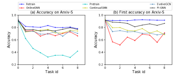
Figure 4. Accuracy on current tasks & task 1 during training.

	Dataset	Arxiv-S		DBLP-S		Paper100M-S
	Metric	PM	FM	PM	FM	PM	FM
Dynamic	EvolveGCN	74.08%.	-5.55%	61.52%	-4.91%	78.14%	-3.17%
Continual	ContinualGNN	75.36%.	-2.17%	62.67%	-0.13%	80.59%	-2.02%
Upper bound	Retrain	81.86%.	-0.12%	64.77%	1.97%	83.42%	-0.64%
SAGE	PI-GNN	77.02%.	-1.22%	64.75%	-0.64%	83.05%	-0.93%
	Distilled PI-GNN	76.50%.	-1.71%	63.49%	-1.11%	82.82%	-1.49%
GCN	PI-GNN	76.85%.	0.93%	63.62%	-0.89%	82.76%	-1.35%
	Distilled PI-GNN	76.11%.	-0.36%	64.09%	0.57%	82.48%	-1.92%
GAT	PI-GNN	78.03%.	1.69%	62.78%	-1.55%	82.99%	-0.75%
	Distilled PI-GNN	76.75%.	-1.27%	62.81%	-1.57%	82.20%	-1.11%

Table 3. Performance Mean (PM) and Forgetting Measure (FM) of different methods for node classification.

We also show the accuracy of PI-GNN and baselines on the current tasks and the first task during the training process in Figure 4. Performance on the current task shows how well the model adapts to new graph patterns, while that on the first task shows how well it maintains knowledge for old graph patterns. We make the following observations:

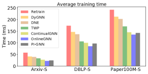
Figure 5. Average training time per epoch

• During the training process, PI-GNN is the closest one to Retrain, which demonstrates the ability of PI-GNN to adapt to new patterns and coincides with our theoretical analysis. OnlineGNN fluctuates greatly because it rewrites parameters and thus suffers from the catastrophic forgetting problem. Pretrain cannot learn new patterns thus it performs worst.

• The performance of ContinualGNN and EvolveGCN gradually drops. We attribute this to the following reasons. ContinualGNN gradually forgets the old knowledge after learning many new patterns because of the constant model capacity, which makes it difficult to accommodate the new patterns using existing parameters without forgetting. EvolveGCN can learn on the whole snapshot, but it aims at capturing dynamism of the dynamic graph and will forget inevitably.

4.3. Efficiency

Figure 5 presents the average training time of PI-GNN per epoch compared with baselines. We do not show the average training time of EvolveGCN because it uses the whole snapshots and RNN to evolve the parameters, which needs more overhead than Retrain. DiCGRL is not shown as it suffers from out of memory problem in Paper100M-S. From the results, we observe that TWP has to calculate the topology weights to preserve structure information and thus results in more overheads. It worth noting that DyGNN and DNE have different settings where they update the nodes embedding after every new edge comes, therefore they have relative large overheads. PI-GNN is as efficient as OnlineGNN. The high efficiency can be attributed to sampling of $G^{t-1}_{memory}$ and incremental learning on $\Delta G^{t}$ and $G_{memory}^{t-1}$ at each snapshot.

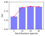
(a) PM for different rectification epochs.

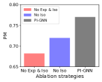
(b) Ablation Study on Isolation and Expansion

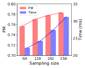
(c) Sample Size of $G_{memory}^{t-1}$

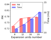
(d) Expansion Units

Figure 6. Analysis Results of PI-GNN.

4.4. Model Analysis

4.4.1. Impact of different backbones

We use different GNN models as the backbones of PI-GNN. The results can be found in Table 3. We only show ContinualGNN and EvolveGCN which have best performance in continual learning methods and dynamic learning methods respectively. We find that our PI-GNN can be combined with different GNN backbones properly.

4.4.2. Knowledge Rectification and Parameter Isolation

First, we study the impact of knowledge rectification. We train different epochs for the knowledge rectification stage and show the results in Figure 6(a). On one hand, we observe a large degradation upon the absence of knowledge rectification (0 epochs), as we may freeze parameters for unstable patterns. On the other hand, the number of epochs has little effect as long as rectification is present.

Second, we perform an ablation study on the parameter isolation stage and show results in Figure 6(b). The significant performance drop upon removal of either parameter isolation or expansion underscores their contribution to PI-GNN.

4.4.3. Hyperparameter Study

We conduct detailed hyperparameter studies on the hyperparameter of our model.

Sampling Size Study. We first study the size of sampling $G_{memory}^{t-1}$. The results are shown in Figure 6(c). We find that sampling more nodes can ensure the tightness of the optimization upper bound. When the upper bound is tight enough, sampling abundant nodes no longer brings additional benefits, but increases the overhead. Therefore, we need to choose a suitable balance between sampling and efficiency. Empirically, we find that good results can be achieved when sampling  1% of the total number of nodes. In our experiments, we sampling 128 nodes for Arxiv-S and 256 for the other datasets empirically (about 1%).

Expansion Units Number Study. We study the influence of expansion units number. As shown in Figure 6(d). We find that a small number (e.g. 12) of units is sufficient as excessive expansion leads to little performance improvement but greater overhead.

Balance Factor Study. We show the influence of balance factor $\beta$ in Table 5 and $\alpha$ in Table 5. We find that improper balance will have some negative influence on the performance.

$\beta$	PM	FM
0	75.96%	-1.17%
0.01	77.02%	-0.22%
0.02	76.95%	-1.61%
0.04	76.99%	-0.87%

Table 4. Influence of $\beta$.

$\lambda$	PM	FM
0	75.24%	1.46%
0.1	77.02%	-1.22%
0.2	77.22%	-0.59%
0.4	76.32%	-1.25%

Table 5. Influence of $\lambda$.

4.5. Layer Output Visualization

To verify our argument that different parameters contribute to capturing different patterns, which serves as the foundation of PI-GNN, we visualize the first layer output of PI-GNN on Arxiv-S dataset. Specifically, we use 20 samples from task 0 and task 2 respectively to show the relationship between different patterns and the first layer output of our model. As shown in Figure 7, the activated neurons are mainly concentrated in the first half for the samples from task 0, and the activated neurons are mainly concentrated in the second half for the samples from task 2, indicating that different parameters contribute to different patterns.

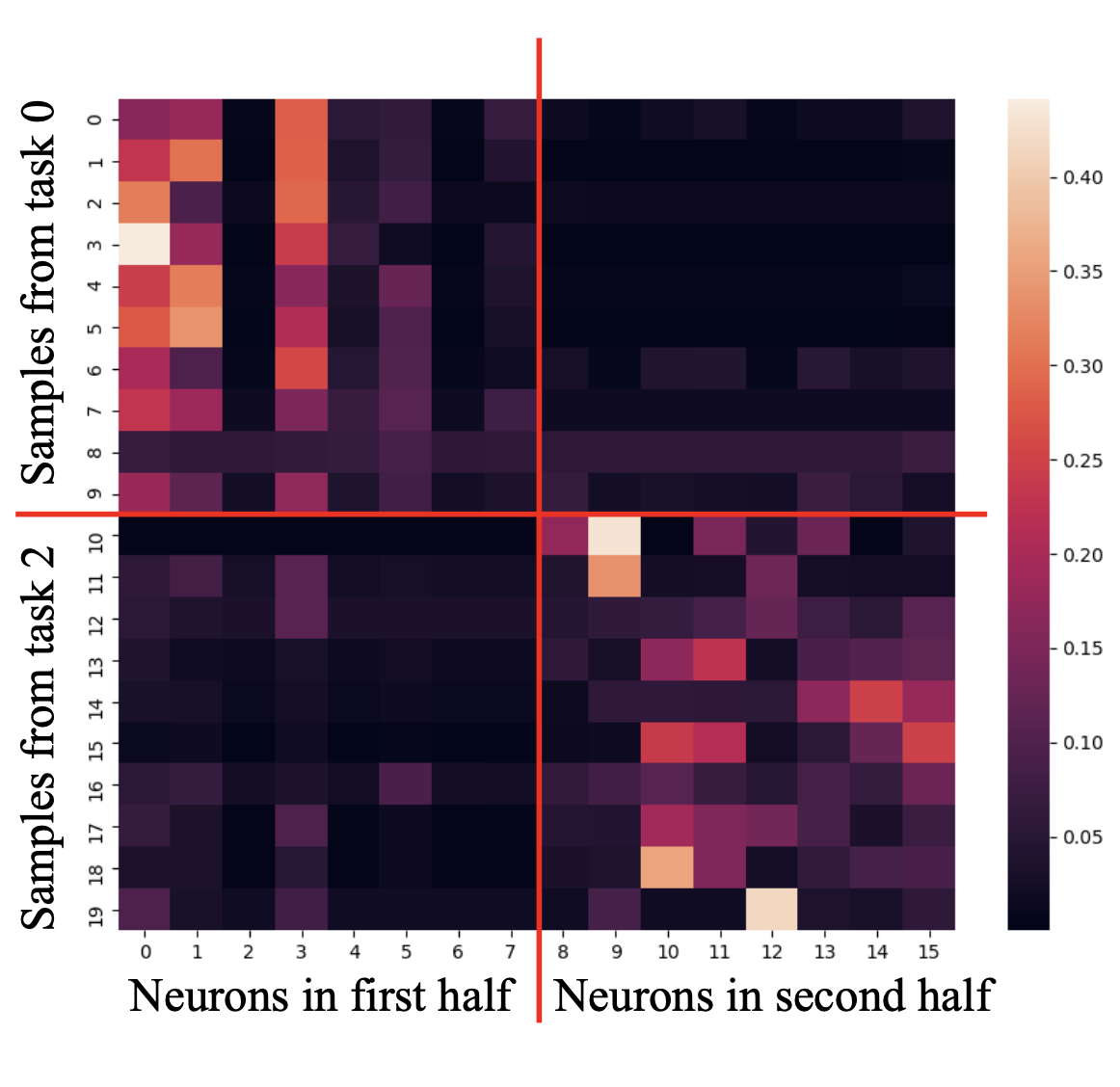
Figure 7. First layer output of samples from different tasks

	Arxiv-S	DBLP-S	Paper100M-S
PI-GNN Size	213KB	759KB.	285KB
Distilled PI-GNN Size	47KB	47KB.	47KB

Table 6. Model size before/after distillation

4.6. Model Compression

Finally, we compare PI-GNN before and after compression along with some baselines. The results are reported in Table 6. We observe that after compression, our model size is reduced by 4× with less than 1% performance drop (shown in Table 2). The results show that PI-GNN can be compressed to avoid being excessively expanded, and thus, PI-GNN is efficient even under large $T$.

5. Related Work

5.1. Dynamic Graph Learning

Most real-world graphs are dynamic with new nodes and edges. Many efforts have been paid to learn representations for dynamic graphs (Goyal et al., 2018; Singer et al., 2019; Hajiramezanali et al., 2019; Kumar et al., 2019). DNE (Du et al., 2018) and DyGNN (Ma et al., 2020) incrementally update node embeddings to reflect changes in graphs. Dyrep (Trivedi et al., 2019) models the micro and macro processes of graph dynamics and fuse temporal information to update node embeddings. EvolveGCN (Pareja et al., 2020) uses recurrent networks to model evolving GNN parameters corresponding to the graph dynamics. However, dynamic graph learning methods in general focus on learning better embeddings for the current and future graphs, rather than previous ones. Consequently, they commonly fail to maintain performance on previous graphs, which is known as catastrophic forgetting.

5.2. Continual Graph Learning

To alleviate catastrophic forgetting in dynamic graphs, researchers propose continual graph learning methods. ER-GNN (Zhou and Cao, 2021) generalizes replay-based methods to GNNs. ContinualGNN (Wang et al., 2020b) proposes importance sampling to store old data for replay and regularization. DiCGRL (Kou et al., 2020) disentangles node representations and only updates the most relevant parts when learning new patterns. TWP (Liu et al., 2021) considers graph structures and preserves them to prevent forgetting. However, all these methods aim to maintain performance on previous graphs while learning for future ones with the same set of parameters with a fixed size. Consequently, a tradeoff between old and new patterns in dynamic graphs has to be made, rendering existing methods sub-optimal.

6. Conclusion

In this paper, we propose PI-GNN for continual learning on dynamic graphs. The idea of PI-GNN naturally fits the unique challenge of continual graph learning. We specifically find parameters that learn stable graph patterns via optimization and freeze them to prevent catastrophic forgetting. Then we expand model parameters to incrementally learn new graph patterns. Our PI-GNN can be combined with different GNN backbones properly. We theoretically prove that PI-GNN optimizes a tight upper bound of the retraining loss on the entire graph. PI-GNN is tested on eight real-world datasets and the results show its superiority.

Appendix A Appendix

A.1. Proof of Lemma 3.2

We show the proof of Lemma 3.2 in this subsection. We first re-state Lemma 3.2:

$L(f_{\theta_{1}}(G)+f_{\theta_{2}}(G))\leq\frac{1}{2}L(f_{\theta_{1}}(G))+\frac{1}{2}L(f_{\theta_{2}}(G))$ where the equality can be established if $f_{\theta_{1}}$ and $f_{\theta_{2}}$ have the same output on $G$.

Proof.

This lemma largely follows from the convexity of $L$ (i.e. cross entropy) and Jensen’s inequality. Here we prove it in detail. For simplicity, we assume that the output dimension of $f_{\theta_{1}}$ and $f_{\theta_{2}}$ are both 2, which can be easily generalized to higher dimensionality. We denote the output of $f_{\theta_{1}}(G)$ as $H_{1}$ where $h^{i}_{1}=(h^{i}_{1,1},h^{i}_{1,2})$ and $h^{i}_{1}$ is the i-th row of $H_{1}$. Similarly, we denote the output of $f_{\theta_{2}}(G)$ as $H_{2}$ where $h^{i}_{2}=(h^{i}_{2,1},h^{i}_{2,2})$and $h^{i}_{2}$ is the i-th row of $H_{2}$

The definition of $L(f_{\theta}(G))$ can be derived as:

(14) $$L\left(f_{\theta}\left(G\right)\right)= \sum_{h^{i}\in H}\mathrm{CrossEnt}\left(\mathrm{softmax}\left(h^{i}\right),y^{i}\right)$$

$$= \sum_{h^{i}\in H}\left\{-y^{i}_{1}\log\left(\frac{e^{h^{i}_{1}}}{e^{h^{i}_{1}}+e^{h^{i}_{2}}}\right)\right.\left.-y^{i}_{2}\log\left(\frac{e^{h^{i}_{2}}}{e^{h^{i}_{1}}+e^{h^{i}_{2}}}\right)\right\}$$

Therefore if we dilate the inequality of Lemma 3.2 according to Equation 14 we will get the formulation which we need to prove as follow:

(15) $$2\sum_{h_{1}^{i}\in H_{1},h_{2}^{i}\in H_{2}}\left\{-y^{i}_{1}\log\left(\frac{e^{h^{i}_{1,1}+h^{i}_{2,1}}}{e^{h^{i}_{1,1}+h^{i}_{2,1}}+e^{h^{i}_{1,2}+h^{i}_{2,2}}}\right)\right.$$

$$\left.-y^{i}_{2}\log\left(\frac{e^{h^{i}_{1,2}+h^{i}_{2,2}}}{e^{h^{i}_{1,1}+h^{i}_{2,1}}+e^{h^{i}_{1,2}+h^{i}_{2,2}}}\right)\right\}$$

$$\leq$$

$$\sum_{h_{1}^{i}\in H_{1}}\left\{-y^{i}_{1}\log\left(\frac{e^{h^{i}_{1,1}}}{e^{h^{i}_{1,1}}+e^{h^{i}_{1,2}}}\right)\right.\left.-y^{i}_{2}\log\left(\frac{e^{h^{i}_{1,2}}}{e^{h^{i}_{1,1}}+e^{h^{i}_{1,2}}}\right)\right\}$$

$$+\sum_{h_{2}^{i}\in H_{2}}\left\{-y^{i}_{1}\log\left(\frac{e^{h^{i}_{2,1}}}{e^{h^{i}_{2,1}}+e^{h^{i}_{2,2}}}\right)\right.\left.-y^{i}_{2}\log\left(\frac{e^{h^{i}_{2,2}}}{e^{h^{i}_{2,1}}+e^{h^{i}_{2,2}}}\right)\right\}$$

Next we prove that for node $i$ this relation holds where we omit $i$ in the following notation, for simplicity, We denote the $h_{1,1},h_{1,2},h_{2,1},h_{2,2}$ as $h_{11},h_{12},h_{21},h_{22}$ respectively. Thus we need prove:

(16) $$-2y_{1}\log\left(\frac{e^{h_{11}+h_{21}}}{e^{h_{11}+h_{21}}+e^{h_{12}+h_{22}}}\right)-2y_{2}\log\left(\frac{e^{h_{12}+h_{22}}}{e^{h_{11}+h_{21}}+e^{h_{12}+h_{22}}}\right)$$

$$\leq -y_{1}\log\left(\frac{e^{h_{11}}}{e^{h_{11}}+e^{h_{12}}}\right)-y_{2}\log\left(\frac{e^{h_{12}}}{e^{h_{11}}+e^{h_{12}}}\right)$$

$$-y_{1}\log\left(\frac{e^{h_{21}}}{e^{h_{21}}+e^{h_{22}}}\right)-y_{2}\log\left(\frac{e^{h_{22}}}{e^{h_{21}}+e^{h_{22}}}\right)$$

$$\Leftrightarrow$$

(17) $$y_{1}\log\left(\frac{\left(e^{h_{11}+h_{21}}\right)^{2}}{\left(e^{h_{11}+h_{21}}+e^{h_{12}+h_{22}}\right)^{2}}\right)+y_{2}\log\left(\frac{\left(e^{h_{12}+h_{22}}\right)^{2}}{\left(e^{h_{11}+h_{21}}+e^{h_{12}+h_{22}}\right)^{2}}\right)$$

$$-y_{1}\log\left(\frac{e^{h_{11}+h_{21}}}{e^{h_{11}+h_{21}}+e^{h_{12}+h_{21}}+e^{h_{11}+h_{22}}+e^{h_{12}+h_{22}}}\right)$$

$$-y_{2}\log\left(\frac{e^{h_{12}+h_{22}}}{e^{h_{11}+h_{21}}+e^{h_{12}+h_{21}}+e^{h_{11}+h_{22}}+e^{h_{12}+h_{22}}}\right)\geq 0$$

$$\Leftrightarrow$$

$$y_{1}\log\left(\frac{1+\frac{e^{h_{12}+h_{21}}+e^{h_{11}+h_{22}}}{e^{h_{11}+h_{21}}+e^{h_{12}+h_{22}}}}{1+\frac{e^{h_{12}+h_{22}}}{e^{h_{11}+h_{21}}}}\right)+y_{2}\log\left(\frac{1+\frac{e^{h_{12}+h_{21}}+e^{h_{11}+h_{22}}}{e^{h_{11}+h_{21}}+e^{h_{12}+h_{22}}}}{1+\frac{e^{h_{11}+h_{21}}}{e^{h_{12}+h_{22}}}}\right)\geq 0$$

We assume that $\frac{e^{h_{12}}}{e^{h_{11}}}=m$, $\frac{e^{h_{22}}}{e^{h_{21}}}=n$, we should prove that:

(18) $$y_{1}\log\left(\frac{1+\frac{m/n+n/m}{1+mn}}{1+mn}\right)+y_{2}\log\left(\frac{1+\frac{m/n+n/m}{1+mn}}{1+\frac{1}{mn}}\right)\geq 0$$

We note that node $i$ can be either in class $y_{1}$ or in class $y_{2}$, Thus:

(1) If node $i$ is labeled with $y_{1}$, which means $y_{1}=1$ and $y_{2}=0$, we have to prove that:

(19) $$\log\left(\frac{1+\frac{m/n+n/m}{1+mn}}{1+mn}\right)\geq 0$$

After optimization we can classify node $i$ rightly, which means that $m\leq 1$ and $n\leq 1$, and thus:

(20) $$\frac{m/n+n/m}{1+mn} \geq 1$$

$$mn \leq 1$$

Therefore, inequality 19 is proved.

(2) If node $i$ is labeled with $y_{2}$, which means $y_{1}=0$ and $y_{2}=1$, we have to prove that:

(21) $$\log\left(\frac{1+\frac{m/n+n/m}{1+mn}}{1+\frac{1}{mn}}\right)\geq 0$$

After optimization we can classify node $i$ rightly, which means that $m\geq 1$ and $n\geq 1$, and thus:

(22) $$m^{2}+n^{2}\geq 1+mn$$

$$\Leftrightarrow \frac{n}{m}+\frac{m}{n}\geq 1+\frac{1}{mn}$$

$$\Leftrightarrow \frac{m/n+n/m}{1+mn}\geq\frac{1}{mn}$$

Therefore, inequality 21 is proved.

In addition, if $m=n$, which means $f_{\theta_{1}}(G)$ and $f_{\theta_{1}}(G)$ have the same output on node $i$, we have:

(23) $$y_{1}\log\left(\frac{1+\frac{m/n+n/m}{1+mn}}{1+mn}\right)+y_{2}\log\left(\frac{1+\frac{m/n+n/m}{1+mn}}{1+\frac{1}{mn}}\right)=0$$

Therefore, Lemma 3.2 is proved. ∎

References

- (1)
- Aljundi et al. (2018) Rahaf Aljundi, Francesca Babiloni, Mohamed Elhoseiny, Marcus Rohrbach, and Tinne Tuytelaars. 2018. Memory aware synapses: Learning what (not) to forget. In Proceedings of the European Conference on Computer Vision (ECCV). 139–154.
- Chaudhry et al. (2018) Arslan Chaudhry, Puneet K Dokania, Thalaiyasingam Ajanthan, and Philip HS Torr. 2018. Riemannian walk for incremental learning: Understanding forgetting and intransigence. In Proceedings of the European Conference on Computer Vision (ECCV). 532–547.
- Du et al. (2018) Lun Du, Yun Wang, Guojie Song, Zhicong Lu, and Junshan Wang. 2018. Dynamic Network Embedding: An Extended Approach for Skip-gram based Network Embedding.. In IJCAI, Vol. 2018. 2086–2092.
- Fernando et al. (2017) Chrisantha Fernando, Dylan Banarse, Charles Blundell, Yori Zwols, David Ha, Andrei A Rusu, Alexander Pritzel, and Daan Wierstra. 2017. Pathnet: Evolution channels gradient descent in super neural networks. arXiv preprint arXiv:1701.08734 (2017).
- French (1999) Robert M French. 1999. Catastrophic forgetting in connectionist networks. Trends in cognitive sciences 3, 4 (1999), 128–135.
- Goyal et al. (2018) Palash Goyal, Nitin Kamra, Xinran He, and Yan Liu. 2018. DynGEM: Deep Embedding Method for Dynamic Graphs. CoRR abs/1805.11273 (2018). arXiv:1805.11273
- Grover and Leskovec (2016) Aditya Grover and Jure Leskovec. 2016. node2vec: Scalable feature learning for networks. In Proceedings of the 22nd ACM SIGKDD international conference on Knowledge discovery and data mining. 855–864.
- Guo et al. (2023) Jiayan Guo, Lun Du, Wendong Bi, Qiang Fu, Xiaojun Ma, Xu Chen, Shi Han, Dongmei Zhang, and Yan Zhang. 2023. Homophily-oriented Heterogeneous Graph Rewiring. arXiv preprint arXiv:2302.06299 (2023).
- Guo et al. (2022a) Jiayan Guo, Yaming Yang, Xiangchen Song, Yuan Zhang, Yujing Wang, Jing Bai, and Yan Zhang. 2022a. Learning Multi-granularity Consecutive User Intent Unit for Session-based Recommendation. In Proceedings of the fifteenth ACM International conference on web search and data mining. 343–352.
- Guo et al. (2022b) Jiayan Guo, Peiyan Zhang, Chaozhuo Li, Xing Xie, Yan Zhang, and Sunghun Kim. 2022b. Evolutionary Preference Learning via Graph Nested GRU ODE for Session-based Recommendation. In Proceedings of the 31st ACM International Conference on Information & Knowledge Management. 624–634.
- Hajiramezanali et al. (2019) Ehsan Hajiramezanali, Arman Hasanzadeh, Krishna R. Narayanan, Nick Duffield, Mingyuan Zhou, and Xiaoning Qian. 2019. Variational Graph Recurrent Neural Networks. In Advances in Neural Information Processing Systems. 10700–10710.
- Hamilton et al. (2017) Will Hamilton, Zhitao Ying, and Jure Leskovec. 2017. Inductive representation learning on large graphs. Advances in neural information processing systems 30 (2017).
- He et al. (2020) Xiangnan He, Kuan Deng, Xiang Wang, Yan Li, Yongdong Zhang, and Meng Wang. 2020. Lightgcn: Simplifying and powering graph convolution network for recommendation. In Proceedings of the 43rd International ACM SIGIR conference on research and development in Information Retrieval. 639–648.
- Hinton et al. (2015) Geoffrey Hinton, Oriol Vinyals, and Jeff Dean. 2015. Distilling the knowledge in a neural network. arXiv preprint arXiv:1503.02531 (2015).
- Huang et al. (2022) Zhongyu Huang, Yingheng Wang, Chaozhuo Li, and Huiguang He. 2022. Going Deeper into Permutation-Sensitive Graph Neural Networks. In International Conference on Machine Learning. PMLR, 9377–9409.
- Hung et al. (2019) Steven CY Hung, Cheng-Hao Tu, Cheng-En Wu, Chien-Hung Chen, Yi-Ming Chan, and Chu-Song Chen. 2019. Compacting, picking and growing for unforgetting continual learning. arXiv preprint arXiv:1910.06562 (2019).
- Jin et al. (2022a) Yiqiao Jin, Yunsheng Bai, Yanqiao Zhu, Yizhou Sun, and Wei Wang. 2022a. Code Recommendation for Open Source Software Developers. In Proceedings of the ACM Web Conference 2023.
- Jin et al. (2023) Yiqiao Jin, Xiting Wang, Yaru Hao, Yizhou Sun, and Xing Xie. 2023. Prototypical Fine-tuning: Towards Robust Performance Under Varying Data Sizes. In Proceedings of the AAAI Conference on Artificial Intelligence.
- Jin et al. (2022b) Yiqiao Jin, Xiting Wang, Ruichao Yang, Yizhou Sun, Wei Wang, Hao Liao, and Xing Xie. 2022b. Towards fine-grained reasoning for fake news detection. In Proceedings of the AAAI Conference on Artificial Intelligence, Vol. 36. 5746–5754.
- Ke et al. (2020) Zixuan Ke, Bing Liu, and Xingchang Huang. 2020. Continual learning of a mixed sequence of similar and dissimilar tasks. Advances in Neural Information Processing Systems 33 (2020), 18493–18504.
- Kipf and Welling (2016) Thomas N Kipf and Max Welling. 2016. Semi-supervised classification with graph convolutional networks. arXiv preprint arXiv:1609.02907 (2016).
- Kirkpatrick et al. (2017) James Kirkpatrick, Razvan Pascanu, Neil Rabinowitz, Joel Veness, Guillaume Desjardins, Andrei A Rusu, Kieran Milan, John Quan, Tiago Ramalho, Agnieszka Grabska-Barwinska, et al. 2017. Overcoming catastrophic forgetting in neural networks. Proceedings of the national academy of sciences 114, 13 (2017), 3521–3526.
- Klicpera et al. (2020a) Johannes Klicpera, Shankari Giri, Johannes T Margraf, and Stephan Günnemann. 2020a. Fast and uncertainty-aware directional message passing for non-equilibrium molecules. arXiv preprint arXiv:2011.14115 (2020).
- Klicpera et al. (2020b) Johannes Klicpera, Janek Groß, and Stephan Günnemann. 2020b. Directional message passing for molecular graphs. arXiv preprint arXiv:2003.03123 (2020).
- Kou et al. (2020) Xiaoyu Kou, Yankai Lin, Shaobo Liu, Peng Li, Jie Zhou, and Yan Zhang. 2020. Disentangle-based Continual Graph Representation Learning. In Proceedings of the 2020 Conference on Empirical Methods in Natural Language Processing (EMNLP). 2961–2972.
- Kumar et al. (2019) Srijan Kumar, Xikun Zhang, and Jure Leskovec. 2019. Predicting Dynamic Embedding Trajectory in Temporal Interaction Networks. In Proceedings of the 25th ACM SIGKDD International Conference on Knowledge Discovery & Data Mining. 1269–1278. https://doi.org/10.1145/3292500.3330895
- Li et al. (2022) Rui Li, Jianan Zhao, Chaozhuo Li, Di He, Yiqi Wang, Yuming Liu, Hao Sun, Senzhang Wang, Weiwei Deng, Yanming Shen, et al. 2022. House: Knowledge graph embedding with householder parameterization. In International Conference on Machine Learning. PMLR, 13209–13224.
- Li and Hoiem (2017) Zhizhong Li and Derek Hoiem. 2017. Learning without forgetting. IEEE transactions on pattern analysis and machine intelligence 40, 12 (2017), 2935–2947.
- Liu et al. (2021) Huihui Liu, Yiding Yang, and Xinchao Wang. 2021. Overcoming Catastrophic Forgetting in Graph Neural Networks. In Proceedings of the AAAI Conference on Artificial Intelligence, Vol. 35. 8653–8661.
- Lopez-Paz and Ranzato (2017) David Lopez-Paz and Marc’Aurelio Ranzato. 2017. Gradient episodic memory for continual learning. arXiv preprint arXiv:1706.08840 (2017).
- Ma et al. (2022) Xiaojun Ma, Qin Chen, Yuanyi Ren, Guojie Song, and Liang Wang. 2022. Meta-Weight Graph Neural Network: Push the Limits Beyond Global Homophily. In Proceedings of the ACM Web Conference 2022. 1270–1280.
- Ma et al. (2020) Yao Ma, Ziyi Guo, Zhaocun Ren, Jiliang Tang, and Dawei Yin. 2020. Streaming graph neural networks. In Proceedings of the 43rd International ACM SIGIR Conference on Research and Development in Information Retrieval. 719–728.
- McCallum et al. (2000) Andrew Kachites McCallum, Kamal Nigam, Jason Rennie, and Kristie Seymore. 2000. Automating the construction of internet portals with machine learning. Information Retrieval 3 (2000), 127–163.
- McCloskey and Cohen (1989) Michael McCloskey and Neal J Cohen. 1989. Catastrophic interference in connectionist networks: The sequential learning problem. In Psychology of learning and motivation. Vol. 24. Elsevier, 109–165.
- Pang et al. (2022) Bochen Pang, Chaozhuo Li, Yuming Liu, Jianxun Lian, Jianan Zhao, Hao Sun, Weiwei Deng, Xing Xie, and Qi Zhang. 2022. Improving Relevance Modeling via Heterogeneous Behavior Graph Learning in Bing Ads. In Proceedings of the 28th ACM SIGKDD Conference on Knowledge Discovery and Data Mining. 3713–3721.
- Pareja et al. (2020) Aldo Pareja, Giacomo Domeniconi, Jie Chen, Tengfei Ma, Toyotaro Suzumura, Hiroki Kanezashi, Tim Kaler, Tao Schardl, and Charles Leiserson. 2020. Evolvegcn: Evolving graph convolutional networks for dynamic graphs. In Proceedings of the AAAI Conference on Artificial Intelligence, Vol. 34. 5363–5370.
- Perozzi et al. (2014) Bryan Perozzi, Rami Al-Rfou, and Steven Skiena. 2014. Deepwalk: Online learning of social representations. In Proceedings of the 20th ACM SIGKDD international conference on Knowledge discovery and data mining. 701–710.
- Ramesh and Chaudhari (2021) Rahul Ramesh and Pratik Chaudhari. 2021. Model Zoo: A Growing Brain That Learns Continually. In NeurIPS 2021 Workshop on Distribution Shifts: Connecting Methods and Applications.
- Ratcliff (1990) Roger Ratcliff. 1990. Connectionist models of recognition memory: constraints imposed by learning and forgetting functions. Psychological review 97, 2 (1990), 285.
- Rebuffi et al. (2017) Sylvestre-Alvise Rebuffi, Alexander Kolesnikov, Georg Sperl, and Christoph H Lampert. 2017. icarl: Incremental classifier and representation learning. In Proceedings of the IEEE conference on Computer Vision and Pattern Recognition. 2001–2010.
- Rolnick et al. (2018) David Rolnick, Arun Ahuja, Jonathan Schwarz, Timothy P Lillicrap, and Greg Wayne. 2018. Experience replay for continual learning. arXiv preprint arXiv:1811.11682 (2018).
- Rosenfeld and Tsotsos (2018) Amir Rosenfeld and John K Tsotsos. 2018. Incremental learning through deep adaptation. IEEE transactions on pattern analysis and machine intelligence 42, 3 (2018), 651–663.
- Rusu et al. (2016) Andrei A Rusu, Neil C Rabinowitz, Guillaume Desjardins, Hubert Soyer, James Kirkpatrick, Koray Kavukcuoglu, Razvan Pascanu, and Raia Hadsell. 2016. Progressive neural networks. arXiv preprint arXiv:1606.04671 (2016).
- Sen et al. (2008) Prithviraj Sen, Galileo Namata, Mustafa Bilgic, Lise Getoor, Brian Galligher, and Tina Eliassi-Rad. 2008. Collective classification in network data. AI magazine 29, 3 (2008), 93–93.
- Shchur et al. (2018) Oleksandr Shchur, Maximilian Mumme, Aleksandar Bojchevski, and Stephan Günnemann. 2018. Pitfalls of graph neural network evaluation. arXiv preprint arXiv:1811.05868 (2018).
- Shi et al. (2021) Guangyuan Shi, Jiaxin Chen, Wenlong Zhang, Li-Ming Zhan, and Xiao-Ming Wu. 2021. Overcoming Catastrophic Forgetting in Incremental Few-Shot Learning by Finding Flat Minima. Advances in Neural Information Processing Systems 34 (2021).
- Shin et al. (2017) Hanul Shin, Jung Kwon Lee, Jaehong Kim, and Jiwon Kim. 2017. Continual learning with deep generative replay. arXiv preprint arXiv:1705.08690 (2017).
- Singer et al. (2019) Uriel Singer, Ido Guy, and Kira Radinsky. 2019. Node Embedding over Temporal Graphs. In Proceedings of the Twenty-Eighth International Joint Conference on Artificial Intelligence, IJCAI-19. 4605–4612. https://doi.org/10.24963/ijcai.2019/640
- Tang et al. (2015) Jian Tang, Meng Qu, Mingzhe Wang, Ming Zhang, Jun Yan, and Qiaozhu Mei. 2015. Line: Large-scale information network embedding. In Proceedings of the 24th international conference on world wide web. 1067–1077.
- Tang et al. (2008) Jie Tang, Jing Zhang, Limin Yao, Juanzi Li, Li Zhang, and Zhong Su. 2008. Arnetminer: extraction and mining of academic social networks. In Proceedings of the 14th ACM SIGKDD international conference on Knowledge discovery and data mining. 990–998.
- Trivedi et al. (2019) Rakshit Trivedi, Mehrdad Farajtabar, Prasenjeet Biswal, and Hongyuan Zha. 2019. Dyrep: Learning representations over dynamic graphs. In International conference on learning representations.
- Veličković et al. (2017) Petar Veličković, Guillem Cucurull, Arantxa Casanova, Adriana Romero, Pietro Lio, and Yoshua Bengio. 2017. Graph attention networks. arXiv preprint arXiv:1710.10903 (2017).
- Wang et al. (2020b) Junshan Wang, Guojie Song, Yi Wu, and Liang Wang. 2020b. Streaming Graph Neural Networks via Continual Learning. In Proceedings of the 29th ACM International Conference on Information & Knowledge Management. 1515–1524.
- Wang et al. (2020a) Kuansan Wang, Zhihong Shen, Chiyuan Huang, Chieh-Han Wu, Yuxiao Dong, and Anshul Kanakia. 2020a. Microsoft academic graph: When experts are not enough. Quantitative Science Studies 1, 1 (2020), 396–413.
- Weber et al. (2019) Mark Weber, Giacomo Domeniconi, Jie Chen, Daniel Karl I Weidele, Claudio Bellei, Tom Robinson, and Charles E Leiserson. 2019. Anti-money laundering in bitcoin: Experimenting with graph convolutional networks for financial forensics. arXiv preprint arXiv:1908.02591 (2019).
- Wu et al. (2019) Felix Wu, Amauri Souza, Tianyi Zhang, Christopher Fifty, Tao Yu, and Kilian Weinberger. 2019. Simplifying graph convolutional networks. In International conference on machine learning. PMLR, 6861–6871.
- Xu et al. (2018) Keyulu Xu, Weihua Hu, Jure Leskovec, and Stefanie Jegelka. 2018. How powerful are graph neural networks? arXiv preprint arXiv:1810.00826 (2018).
- Yang et al. (2022) Ruichao Yang, Xiting Wang, Yiqiao Jin, Chaozhuo Li, Jianxun Lian, and Xing Xie. 2022. Reinforcement subgraph reasoning for fake news detection. In Proceedings of the 28th ACM SIGKDD Conference on Knowledge Discovery and Data Mining. 2253–2262.
- Yoon et al. (2017) Jaehong Yoon, Eunho Yang, Jeongtae Lee, and Sung Ju Hwang. 2017. Lifelong learning with dynamically expandable networks. arXiv preprint arXiv:1708.01547 (2017).
- Zenke et al. (2017) Friedemann Zenke, Ben Poole, and Surya Ganguli. 2017. Continual learning through synaptic intelligence. In International Conference on Machine Learning. PMLR, 3987–3995.
- Zhang et al. (2023) Peiyan Zhang, Jiayan Guo, Chaozhuo Li, Yueqi Xie, Jae Boum Kim, Yan Zhang, Xing Xie, Haohan Wang, and Sunghun Kim. 2023. Efficiently Leveraging Multi-level User Intent for Session-based Recommendation via Atten-Mixer Network. In Proceedings of the Sixteenth ACM International Conference on Web Search and Data Mining. 168–176.
- Zhang and Kim (2023) Peiyan Zhang and Sunghun Kim. 2023. A Survey on Incremental Update for Neural Recommender Systems. arXiv preprint arXiv:2303.02851 (2023).
- Zhang et al. (2022) Yiding Zhang, Chaozhuo Li, Xing Xie, Xiao Wang, Chuan Shi, Yuming Liu, Hao Sun, Liangjie Zhang, Weiwei Deng, and Qi Zhang. 2022. Geometric Disentangled Collaborative Filtering. In Proceedings of the 45th International ACM SIGIR Conference on Research and Development in Information Retrieval. 80–90.
- Zhao et al. (2022) Jianan Zhao, Meng Qu, Chaozhuo Li, Hao Yan, Qian Liu, Rui Li, Xing Xie, and Jian Tang. 2022. Learning on Large-scale Text-attributed Graphs via Variational Inference. arXiv preprint arXiv:2210.14709 (2022).
- Zhou and Cao (2021) Fan Zhou and Chengtai Cao. 2021. Overcoming Catastrophic Forgetting in Graph Neural Networks with Experience Replay. In Proceedings of the AAAI Conference on Artificial Intelligence, Vol. 35. 4714–4722.