Leveraging Uncertainty Quantification for Picking Robust First Break Times

Abstract

In seismic exploration, the selection of first break times is a crucial aspect in the determination of subsurface velocity models, which in turn significantly influences the placement of wells. Many deep neural network (DNN)-based automatic first break picking methods have been proposed to speed up this picking processing. However, there has been no work on the uncertainty of the first picking results of the output of DNN. In this paper, we propose a new framework for first break picking based on a Bayesian neural network to further explain the uncertainty of the output. In a large number of experiments, we evaluate that the proposed method has better accuracy and robustness than the deterministic DNN-based model. In addition, we also verify that the uncertainty of measurement is meaningful, which can provide a reference for human decision-making.

I Introduction

Detecting the first break times of P-wave or S-wave in pre-stack seismic gather is a crucial problem in seismic data processing. Accurate first break pickings can provide precise static correction results, then greatly improve the quality of subsequent seismic data processing[1], e.g., velocity analysis, stratigraphic imaging, etc. With the increase of seismic data acquisition density, the efficiency of manually first break picking is far behind the speed of acquisition. Thus, the automatic first break picking algorithm has become a key problem in reducing the seismic processing period.

In the initial exploration of the automatic picking methods, many methods recognize the first break time based on the signal characteristics near the first break time, such as energy ratio-based methods[2][3][4][5], higher-order statistics-based methods[6][7], etc. Concretely, taking the feature named the short- and long-time average ratio (STA/LTA)[2][3] as an example, the local feature of a single trace is calculated by sliding window, and then the time point whose STA/LTA value is first larger than the threshold set in advance is taken as the first break time. Then, considering the correlation between multiple signals, using the correlation coefficient is proposed to identify the first break times[8][9]. Later, the feature signal extraction method of multiple signals is proposed one after another[10][11][12].

Recently, machine learning and deep learning have shown high efficiency and strong practicability in computer vision, natural language processing, and other fields. The deep learning method has a strong ability to represent complex functions, which greatly makes up for the low complexity of feature extraction in traditional first break picking methods. Thus, a large number of the automatically first break picking methods based on machine learning and deep learning have been proposed. In general, current popular methods can be divided into three classes: clustering method-based methods, local image classification-based methods, and end-to-end segmentation-based methods.

First, the clustering-based picking method generally transforms seismic signal data into other domains, then uses the clustering methods to split the clusters, and finally defines the boundary of two clusters as the first break time. Concretely, Xu et al. [13] proposed a multi-stage clustering-based method, which first determines the first-break time window, then utilizes an improved clustering method to obtain the initial first break times of every single trace, and finally considers comprehensively the picking results of the near traces to refine the pickings. Then, Gao et al. [14] considered the clustering methods based on a shot-gather (multiple signals level) to enhance the correlation of automatic pickings among the near traces. Currently, Lan et al. [15] proposed a more complex and robust automatic picking method based on fuzzy C means clustering (FCM) and Akaike information criterion (AIC) to further improve the accuracy and robustness of clustering-based methods. Second, the local image classification-based methods first split the whole shot gather image into a few mini-patch and then utilize neural networks (NN) or machine learning classification methods to classify the mini-patch sub-image into two classes, i.e., FB or non-FB. At a very early time, McCormack et al. [16] proposed the use of a fully connected network (FCN) to complete the binary classification task. Then, FCN was replaced by convolutional neural networks (CNN) for image classification to improve classification accuracy[17]. Different from classification for picking FB directly, Duan et al. [18] first obtain a preliminary picking result based on the traditional picking method and then utilize CNN to identify poor picks. Currently, Guo et al. [19] combined more feature information as the input of the classifier and proposed a new post-processing method to improve the stability of the picking results. Compared to NN-based methods, the classic machine learning-based methods outperform in a small sample size scenario, e.g., support vector machine (SVM)[20], support vector regression (SVR), and extreme gradient boosting (XGBoost)[21]. Third, end-to-end segmentation-based methods are currently the most popular automatic picking methods since fully convolutional networks (FCN)[22] and U-Net[23] are widely used for pixel-level segmentation and have excellent segmentation accuracy. Concretely, FCN was applied to segment the first break part in the image of a shot gather, and the techniques of semi-supervised learning and transfer learning were conducted to learn a better high-level feature[24][25][26]. Then, U-Net, an excellent medical image segmentation tool, was utilized to solve the segmentation task of labeling the first break times[27][28][29][30]. Yuan et al. [31] further proposed post-processing to refine the U-Net-based picking results, where conducts a recurrent neural network (RNN) to regress the first break times for every trace. Moreover, the popular transformer has also been used for the segmentation task with respect to picking the first break[32].

Up to now, the method based on semantic segmentation is the most practical and efficient and has been well evaluated in practical applications. Unfortunately, deep neural network (DNN) has always been a black-box model, and we cannot explain the specific role of each layer of the neural network[33]. Therefore, there is no guarantee that the output of neural networks will be correct. However, the principle of the first break-picking task is to put quality before quantity, i.e., the accuracy should be guaranteed even if the pick rate is reduced[1]. In order to solve the security problem of automatic first break pickings, we introduce the concept of uncertainty qualification into the picking task based on segmentation networks. Uncertainty qualification methods measure two parts of uncertainty, epistemic uncertainty (model uncertainty) and aleatoric uncertainty (data uncertainty)[34]. In this paper, we focus on the epistemic uncertainty of the segmentation neural network, where the main task is modeling and solving the posterior distribution of the model weights. With the proposed methods of Monte Carlo (MC) dropout[35], Bayes by Backprop (BBB) [36], and deep ensemble[37], the computational cost of the uncertain qualification methods is greatly reduced and the generalization accuracy of the model is dramatically improved. Further, uncertainty qualification methods are extended to semantic segmentation[38], especially to the segmentation tasks of medical images[39][40] and remote sensing images[41]. Although there have been many application methods based on uncertainty qualification, no uncertainty qualification method is fully applicable to the first break picking based on the segmentation network.

This article proposes a new framework for measuring the uncertainty of the first break pickings as shown in Fig. 1. First, we conduct pre-processing including reducing input size and enhancing the first break feature. Then, we combine U-Net and MC dropout to achieve a posterior inference network. Finally, we propose a post-processing method based on the uncertainty qualification to obtain robust first-break pickings.

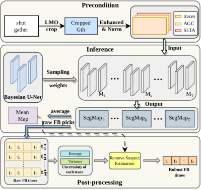
Figure 1: The main flow chart of a new framework we propose to pick FB times robustly.

II Preliminary

II-A Problem Statement

Primarily, first break picking is a problem of detecting the first changed point which indicates a first arrival wave event in the seismic signal data. For instance, the red dash line (Fig. 2, left) labels the first break time since there is the first trough. Generally, the peak or trough of the first break time is determined by the source. In a higher scale view, the first break times of the adjacent signals on a shot gather usually have a stronger correlation as shown in the right subfigure of Fig. 2. Based on the spatial characteristics of the first break mentioned above, we define the first break picking as a statistical inference problem $P(\mathbf{t}|\mathbf{G})$, which infers a time series $\mathbf{t}$ of the first break based on the shot gather $\mathbf{G}$.

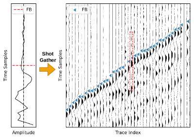
Figure 2: Showcase of the first break times. The left subfigure shows t he first break time of a single trace. The right subfigure indicates the high correlation of the first break times of the adjacent traces. The red dotted box marks the location of the single channel signal on the left subfigure.

II-B Uncertainty Qualification for First Break Picking

We transform the picking model to a probability model to introduce uncertainty to the first break picking. In view of statistic, the first break inference $P(\mathbf{t}|\mathbf{G})$ can be described as solving a maximum posterior estimation:

$$\mathbf{\hat{t}}=\arg\max_{\mathbf{t}}\{P(\mathbf{t}|\mathbf{G},\mathcal{D})\},$$ (1)

where, $\mathbf{t}$ is a time series of the first break, $\mathbf{G}$ is a shot gather, and $\mathcal{D}$ is the annotation knowledge of the first break, i.e., the labeled dataset. In this paper, we only consider the model uncertainty, i.e., epistemic uncertainty, in the inference model (Eq. 1). Concretely, the model weights $w$ are assumed to follow a posterior distribution $P(w|\mathcal{D})$. Therefore, the posterior distribution can be expressed by a form of marginal average:

$$P(\mathbf{t}|\mathbf{G},\mathcal{D})=\int_{w}{P(\mathbf{t}|\mathbf{G},w)\cdot P(w|\mathcal{D})dw},$$ (2)

where $P(\mathbf{t}|\mathbf{G},w)$ is an inference model with weights $w$.

However, the true posterior $P(w|\mathcal{D})$ is intractable, and we have to utilize other techniques to approximate it, e.g., variational inference (VI)[42], which minimizes the Kullback–Leibler (KL) divergence between the true posterior $P(w|\mathcal{D})$ and an approximation distribution $q(w)$:

$$KL\left[q(w)||P(w|\mathcal{D})\right]=\int q(w)\ln\frac{q(w)}{P(w|\mathcal{D})}dw$$ (3)

Then, we maximize the evidence low bound (ELBO) deduced by Eq. 3 to optimize the approximation distribution $q(w)$:

$$\text{ELBO}(q)=KL\left[q(w)||P(w,\mathcal{D})\right]-\ln P(\mathcal{D}).$$ (4)

However, traditional VI-based methods are inefficient to optimize Eq. 4 and are hard to directly apply to deep learning-based methods. Fortunately, Gal and Ghahramani[35] claimed that Monte Carlo dropout applied in a deep neural network can be approximated to a VI processing. The dropout technique is usually used to avoid the overfitting performance of training processing and is only conducted in training processing. Being different from only using in training processing, [35] enables the neural network model to a posterior probability model with the help of dropout layers. Concretely, the dropout technique defines a series of Bernoulli variables $z$ and multiple it by the weight matrix $M$ of a full-connection or convolutional layer, e.g., $M_{i}$ is the weight matrix of the $i$th layer, that is,

$$W_{i}=M_{i}\cdot\text{diag}(\left[z_{i,j}\right]_{j=1}^{K_{i}})$$ (5)

$$z_{i,j}\thicksim Bernoulli(p_{i}),i=1,...,L,j=1,..,K_{i-1}$$ (6)

where $p_{i}$ is the dropout rate of $i$th layer, $L$ is the number of layers, and $K_{i}$ is the number of neural units of $i$th layer. Further, Gal and Ghahramani[35] proved that NN with the dropout technique is a posterior probability model. Next, we inspect the posterior distribution of the model output $\mathbf{t^{*}}\thicksim q(\mathbf{t^{*}}|\mathbf{G^{*}},\mathcal{D})$. The predicted results can be obtained by sampling the model weights $T_{s}$ times from $q(w|\mathcal{D})$ and then calculating every picked result:

$$\mathbf{\hat{t^{*}_{k}}}=f_{w_{k}}(\mathbf{G^{*}}),k=1,...,T_{s},$$ (7)

where $f(\cdot)$ is an inference model for the first break picking. Particularly, the above sampling is sampling $z$ in Eq. 6. The statistical characteristics of the posterior distribution $q(\mathbf{t^{*}}|\mathbf{G^{*}},\mathcal{D})$, e.g., mean, var, and entropy, are estimated by Monte Carlo methods. Thus, Gal and Ghahramani[35] noted this type of dropout as the MC dropout. First, the mean can be inferred using the average of sampled predicts:

$$\text{Mean}(\mathbf{{t^{*}}})=E_{q}\left[\mathbf{{t^{*}}^{2}}\right]\approx\sum\limits_{k=1}^{T_{s}}{\mathbf{\hat{t^{*}_{k}}}}^{2},$$ (8)

where $\mathbf{\hat{t^{*}_{k}}}$ is the $k$th sampled prediction (defined by Eq. 7), $E_{q}\left[\cdot\right]$ means the expectation based on the posterior distribution $q(\mathbf{t^{*}}|\mathbf{G^{*}},\mathcal{D})$, and $T_{s}$ is the sampling times. Momentously, the mean of $\mathbf{{t^{*}}}$ usually is a robust prediction of Bayesian NN and we also take it as the final output of NN in this paper. More importantly, the uncertainty of the first break can be captured by estimating the variance and entropy of $\mathbf{t^{*}}$ using the Monte Carlo method as well. Concretely, the variance of $j$th element of $\mathbf{t^{*}}$ is estimated by:

$$\text{Var}({t_{j}^{*}})=E_{q}\left[{t_{j}^{*}}^{2}\right]-\left[E_{q}{t_{j}^{*}}\right]^{2}\approx\sum\limits_{k=1}^{T_{s}}{\hat{t^{*}_{j,k}}}^{2}-\left[\sum\limits_{k=1}^{T_{s}}{{\hat{t^{*}_{j,k}}}}\right]^{2}$$ (9)

where $\hat{t^{*}_{j,k}}$ is the $j$th element of $k$th sampled prediction (Eq. 7). Particularly, we discrete the time dimension as the finite time points (the number is $C$), so the inference problem defined in Eq. 1 is a classification problem. Therefore, the entropy of $j$th element of $\mathbf{t^{*}}$ is calculated by:

$$\begin{array}[]{c}\text{H}({t_{j}^{*}})=\sum\limits_{c=1}^{C}{-Q_{t_{j}^{*}}(c)\log_{2}Q_{t_{j}^{*}}(c)}\\ \text{with,}\ Q_{t_{j}^{*}}(c)=P\{t_{j}^{*}=c\}\approx\frac{1}{T_{s}}\sum\limits_{k=1}^{T_{s}}{I\{\hat{t^{*}_{j,k}}=c\}}\end{array}$$ (10)

where $Q_{t_{j}^{*}}(c)$ is the posterior probability of $t_{j}^{*}$ equal to the discrete-time $c$ and $I\{\cdot\}$ is the indicator function.

III Methodology

In this section, we will introduce our proposed robustly picking method in detail. As Fig. 1 shown, our approach contains three parts to obtain the robust picking results: precondition, inference by Bayesian U-Net, and post-processing. Next, we introduce the principles of each component in turn.

III-A Data Precondition

We conduct three steps of precondition on the shot gather $\mathbf{G}$: linear moveout (LMO) correction, enhanced feature calculation, and trace-wise normalization. First, we crop the input region of the gather based on the LMO correction, which utilizes a velocity prior of the current survey to estimate reference arrival times for each trace. Especially, the reference arrival time of the $j$th trace $t_{j}$ is computed by:

$$t_{j}=d_{j}/v+t_{0}$$ (11)

where, $d_{j}$ is the offset, i.e., the distance between the source and the receiver. $v$ and $t_{0}$ are the reference velocity and the interception time of the prior information in the current survey, which is detailed in III.B. Therefore, the top boundary and bottom boundary of the crop index of $j$-th trace are $t_{j}-d/2$ and $t_{j}+d/2$, respectively, and the cropped length is $d+1$.

Second, the amplitude gain control (AGC) method and the short- and long-time average ratio (SLTA) method, two useful enhanced techniques for detecting the first arrival times, are conducted on the 2-D gather to highlight the locations of the arrival times as the same as the single-trace picking method[2]. Concretely, both inputs of the above two feature computations are the cropped gather $G_{T\times N}$, i.e., a 2-D array with T rows and N columns, where $T$ and $N$ are the numbers of sampling times and traces. The AGC feature map $F_{\text{AGC}_{T\times N}}$ is computed by the follow:

$$F_{\text{AGC}_{ij}}=\left\{{\begin{array}[]{rl}\frac{1}{w+1}\sum\limits_{k=i-\frac{w}{2}}^{i+\frac{w}{2}}{|G_{kj}|}&\begin{array}[]{l}i=\frac{w}{2},...,T-\frac{w}{2},\\ j=1,...,N,\end{array}\\ 0,&other\end{array}}\right.,$$ (12)

where $G_{kj}$ is the $k$th row and $j$th column element of the cropped gather $G_{T\times N}$, and $w+1$ is the length of sliding window. The SLTA feature map $F_{\text{SLTA}_{T\times N}}$ is calculated by the follow:

$$F_{\text{SLTA}_{ij}}=\left\{{\begin{array}[]{rl}\frac{{n_{l}}\sum\limits_{k=i-{n_{s}}}^{i}{\left|{G}_{kj}\right|}}{{n_{s}}\sum\limits_{k=i-{n_{l}}}^{i}{\left|{G}_{kj}\right|}},&\begin{array}[]{l}i=n_{l},...,T-n_{l},\\ j=1,...,N,\end{array}\\ 0,&other\end{array}}\right.,$$ (13)

where $G_{kj}$ is the $k$-th row and $j$-th column element of the cropped gather $G_{T\times N}$, and $n_{s}$ and $n_{l}$ are the length of the short-time window and long-time window, respectively. As we can see from Fig. 3, AGC can balance the local amplitude for every trace, helping detect the weak signals of the arrival times, and SLTA can stick out the arrival times from the noise part at the beginning signal.

Finally, each feature map is normalized to the range $\left[-1,1\right]$ since the scales of the amplitude of each trace are different caused by various offsets or multiple noises. We conduct a trace-wise normalization method. Definitely, the the $i$-th row and $j$-th column element in the normalized map $\tilde{F}_{T\times N}$ is computed by:

$$\tilde{F}_{ij}=\frac{F_{ij}}{\max_{k=1,...,T}\{F_{kj}\}},i=1,...,T,j=1,...,N,$$ (14)

where ${F}_{i(k)j}$ is the $i(k)$-th row and $j$-th column element of the feature map $F_{T\times N}$. We normalize the crop gather $G_{T\times N}$, the AGC feature map $F_{\text{AGC}_{T\times N}}$, and the SLTA feature map $F_{\text{SLTA}_{T\times N}}$, respectively. Finally, these three normalized maps are concatenated forming a three-channel image with a shape of $3\times T\times N$.

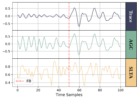
Figure 3: The trace-wise normalized single of three input features: original trace, AGC feature, and SLTA feature. The first break time is labeled by the red dashed line.

III-B Bayesian U-Net

In our work, we choose a popular semantic segmentation model, U-Net[23], combined with the dropout technique as the inference model, aiming to class the first-break position or the non-first-break position on a pixel-level based on the enhanced shot gather maps. Since MC dropout is a Bayesian approximating posterior method[35], we denote the U-Net with MC dropout as Bayesian U-Net (BU-Net), and the network structure is shown in Fig. 4.

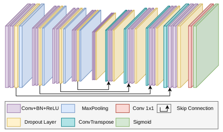
Figure 4: Bayesian U-Net: a U-Net with the MC dropout technique. The input of BU-Net is a three-channel tensor consisting of three normalized feature maps, i.e., the cropped gather (LMO correction, Eq. 11), the AGC map (Eq. 12), and the SLTA map (Eq. 13). The final output is a segmentation map, which indicates the first break position (pixels labeled 1) or non-first break position (pixels labeled 0).

The base model U-Net we use is a fully convolutional neural network with the design of encoder-decoder and skip-connection and in this paper the depth is 4, i.e., conducting down-sampling and up-sampling four times. The convolutional (Conv) layers, Batch-Normal (BN) layers, ReLU activation layers, Max-Pooling layers, dropout layers, transposed convolution (ConvTranspose) layer, and Sigmoid layer are the main component of the BU-Net. The convolutional unit is repeated many times (purple layer in Fig. 4) in the whole processing, consisting of a Conv layer (3$\times$3 kernel, striding $=$ 1, and padding $=$ 1), a BN layer, and a ReLU activation layer. The dropout layers with a constant dropout rate are conducted after each twice convolutional unit. In the encoder part, the Max-Pooling layers (striding $=$ 2) are used to downsample, compressing the redundant information. In the decoder part, we utilize ConvTranspose layers to up-sample, whose kernel size $=$ 2$\times$2 and stride $=$ 2. The skip connections are also used to concatenate the decoded features and original shallow encoded features, aiming to better recover the details of the segmentation. Finally, we use a Conv layer with 1$\times$1 kernel, to compress and summarize the decoded outputs without changing the output shape, and a Sigmoid layer to normalize the segmentation map in the range of $\left[0,1\right]$. Moreover, the kernel numbers of each Conv layer should be underlined, which are equal to the number of output channels, and there are 19 Conv layers, whose kernel numbers are 64, 64, 128, 128, 256, 256, 512, 512, 512, 512, 256, 256, 128, 128, 64, 64, 64, 64, and 1, respectively.

Since Bayesian U-Net is a probability model, we first sample the model weights many times when we infer the first break of a shot gather unseen before:

$$f_{w_{k}}=\text{BUNet}_{w_{k}},w_{k}\backsim p(w|\mathcal{D}),k=1,...,T_{s},$$ (15)

where $f_{w_{k}}$ is the BU-Net with the model weight $w_{k}$, which is sampled from the posterior distribution $p(w|\mathcal{D})$ (in Eq. 2), and $T_{s}$ is the sampling time. Explicitly, the sampling processing is defined as that Bernoulli variables of dropout layers are sampled from a Bernoulli distribution with a successful probability equal to the dropout rate. Then, we can input the enhanced feature maps $\mathbf{G^{*}}$ into these $T_{s}$ sampled models $f_{w_{1}},...,f_{w_{T_{s}}}$ and obtain $T_{s}$ segmentation maps $S_{1},...,S_{T_{s}}$:

$$S_{k}=f_{w_{k}}(\mathbf{G^{*}}),k=1,2,...,T_{s},$$ (16)

where $\mathbf{G^{*}}$ is a three-channel tensor in Eq. 7, which is composed of the cropped gather (LMO correction, Eq. 11), the AGC map (Eq. 12), and the SLTA map (Eq. 13). Segmentation maps $S_{1},...,S_{T_{s}}$ indicate the positions of first breaks, whose segmentation values are close to 1. Importantly, the inference processes of these $T_{s}$ models are independent of each other. As long as the memory width of the calculation cards of computers allows, these inference processes can run in parallel. Naturally, we compute an average map $\bar{S}$ (named Mean Map in Fig. 1) based on segmentation maps $S_{1},...,S_{T_{s}}$ to obtain a stable estimation map:

$$\bar{S}_{ij}=\frac{1}{T_{s}}{\sum\limits_{k=1}^{T_{s}}{S_{k_{ij}}}},i=1,...,T,j=1,...,N$$ (17)

where $\bar{S}_{ij}$ and $S_{k_{ij}}$ are the $i$th-row and $j$th-column element of the average map$\bar{S}$ and $k$th segmentation map $S_{k}$, respectively, and $T$ and $N$ is the height and width of the input image, respectively. Then, we can get the initial robust FB picking $\mathbf{\hat{t^{*}}}$ of each trace:

$$\hat{t^{*}_{j}}=\left\{\begin{array}[]{cl}\arg\max_{i}\{\bar{S}_{ij}\},&j\in\{j|\max_{i}\{\bar{S}_{ij}\}>T_{p}\},\\ -1,&\text{other},\end{array}\right.$$ (18)

where $\hat{t^{*}_{j}}$ is the picked FB time sample index of $j$th trace ($j\in\{1,2,...,N\}$), $T_{p}$ is the picking threshold, $N$ is the number of the traces, and $\hat{t^{*}_{j}}=-1$ means we reject to pick the $j$th trace. So far, we get a stable pickup result initially.

III-C Post-processing

Although the initial picking $\mathbf{\hat{t^{*}}}$ (in Eq. 18) is a stable pickup result, there are a few FB points with low confidence values picked. Thus, we conduct post-processing to remove the suspect estimation so that we can reduce the uncertainty of the whole picking results of a shot gather. To measure the uncertainty in the inference results $S_{1},...,S_{T_{s}}$, we first select the FB times $\hat{t}^{(k)}_{j},j=1,...,N$ from each segmentation map $S_{k}$ using the same method as Eq. 18. Then, we can calculate the variance vector $E$ and the entropy vector $V$ of the picking results of each trace using Eq. 9 and Eq. 10, respectively. Intuitively, we remove the FB pickings with high-uncertainty values by:

$$\tilde{t^{*}_{j}}=\left\{\begin{array}[]{cl}\hat{t^{*}_{j}},&j\in\{j|E_{j}<T_{E}\text{\&}V_{j}<T_{V}\},\\ -1,&\text{other},\end{array}\right.$$ (19)

where $\tilde{t^{*}_{j}}$ is the picked FB time sample index of $j$th trace ($j\in\{1,2,...,N\}$), $E_{j}$ and $V_{j}$ are the entropy and variance of picking of the $j$th trace, respectively, $T_{E}$ and $T_{V}$ are the allowed max uncertainty threshold of entropy and variance, respectively, $\tilde{t^{*}_{j}}=-1$ also means we reject to pick the $j$th trace. Finally, we correct the FB time to the nearest peak or trough based on the source type in order to keep the stability of automatically picking.

IV Experiments

IV-A Datasets and Metrics

To facilitate comparison of other popular methods and other researchers expediently reproduce our approach, we test on a group of the open source field datasets from all unique mining sites in three provinces of Canada provided by [29], including four datasets, named Lalor, Brunswick, Halfmile, and Sudbury, respectively. More details of each dataset are shown in Tab. I, in which label ratio is the ratio of the number of labeled traces to the number of all traces. The provided first break time labels are first obtained using the SLTA method and then corrected by experts. Moreover, each break time of four datasets is annotated at the trough of a waveform.

TABLE I: Open dataset information

Survey	Shot Gather Num.	Label Ratios	Sample Interval	Sample Times
Brunswick (B)	18475	83.54%	2ms	751
Lalor (L)	14455	46.13%	1ms	1001
Sudbury (S)	11420	12.9%	2ms	751
Halfmile (H)	5520	90.35%	2ms	1001

We set three metrics to measure the picking results of different models. In particular, manual picking does not pick the FB times of all traces, so we only consider the regions picked both manually and automatically when evaluating the accuracy. To avoid picking too little, we also consider the pick rate to evaluate the pick rate of the automatic picking method. The first metric is the mean absolute error (MAE), which measures the mean deviation of the time sampling between the automatic picking and the manual picking:

$$\text{MAE}(\mathbf{t_{A}},\mathbf{t_{M}})=\frac{\sum\limits_{j=1}^{N}{|t_{A_{j}}-t_{M_{j}}|\cdot I\{t_{A_{j}},t_{M_{j}}>0\}}}{\sum\limits_{j=1}^{N}{I\{t_{A_{j}},t_{M_{j}}>0\}}},$$ (20)

where $\mathbf{t_{A}}$ and $\mathbf{t_{M}}$ are the shot picking results of the automatic picking and the manual picking, respectively, $t_{A_{j}}$ is the automatic picking of the $j$th trace (no picking $t_{A_{j}}=-1$), $N$ is the traces number of a shot gather, and $I(\cdot)$ is the indicator function. The second one, accuracy (ACC), is used for evaluating the average accuracy of automatic picking in a shot gather:

$$\text{ACC}(\mathbf{t_{A}},\mathbf{t_{M}})=\frac{\sum\limits_{j=1}^{N}I\{t_{A_{j}}=t_{M_{j}};t_{A_{j}},t_{M_{j}}>0\}}{\sum\limits_{j=1}^{N}{I\{t_{A_{j}},t_{M_{j}}>0\}}}.$$ (21)

The last metric is the automatic picking rate (APR), which indicates the picking ratio between the numbers of automatic picking and all traces:

$$\text{APR}(\mathbf{t_{A}})=\frac{1}{N}{\sum\limits_{j=1}^{N}I\{t_{A_{j}}>0\}}.$$ (22)

IV-B Implement Details

This subsection will describe the implementation details of the model’s hyper-parameter selection and training setting. We first reintroduce the important model hyperparameters of data precondition and post-processing and the following parameter selection is based on a large number of experimental verification. In data precondition, the window width of AGC ($w$ in Eq. 12) is set as 30 time samples, and the lengths of the short window and long window ($n_{s}$ and $n_{l}$ in Eq. 13) are set as 3 and 5 time samples. Next, the structure of the implemented Bayesian U-Net is the same as that described in III.B. Then, there are two thresholds ($T_{E}$ and $T_{V}$ in Eq. 19) in post-processing with respect to the allowed maximum of entropy and variance which are set as $T_{E}=0.2$ and $T_{V}=0.2$, respectively.

Bayesian U-Net is a supervised model, so we design three training types according to the practical application needs: single-survey training, cross-survey training, and pretraining&finetuning training. The main difference between the above three training types is that the data sets are divided differently. First, single-survey training means that we divide randomly a single dataset into a training set, a validation set, and a test set by 0.6: 0.2: 0.2. This training type is suitable for picking the survey with a large number of annotations of first break times. Then, the cross-survey training set two surveys as the training set, a survey as the validation set, and the last survey as the test set. The purpose is obvious we want to pick the survey without any labels. The last type is the pretraining&finetuning training method, where the samples of three surveys are divided randomly into a training set and a validation set for pretraining, and the pretrained model is fine-tuned on the last survey. Specifically, in finetuning processing, the sets of training, validation, and test are split as the same as the single-survey training, but only a small number of samples in the training set, 50 samples in this paper, have been applied in training. Obviously, when we have a sufficiently large annotated data set, we are more likely to train a highly generalized pre-training model. When predicting the new survey, we choose to pick manually a small number of samples for finetuning and improve the generalization accuracy under the new survey. More details of the data partition are shown in Tab. II, where the H, B, L, and S are uppercase of the dataset names.

TABLE II: Data Partition of Three Training Types

Training Types	Training Set	Validation Set	Test Set
Single-survey	H(60%)	H(20%)	H(20%)
Cross-survey	[B, L](100%)	S(100%)	H(100%)
Pretraining	[B, L, S](60%)	[B, L, S](20%)	-
Fine-tuning	50 shots in H(60%)	H(20%)	H(20%)

In training processing, we consider these hyperparameters as shown in Tab. III: loss functions, the size of the input image (Input Size), the size of the training mini-batch (Batch Size), the learning rate of the optimizer (Init Lr), optimizer (Optim), and the dropout rate (Dropout Rate). In order to speed up the efficiency of hyper-parameter selection, we choose to select parameters in the experimental scene of the single-survey training type. Concretely, these hyper-parameter combinations of Tab. III are tested by a grid searching method. We performed model training ten times with ten fixed initialization seeds for each set of parameter combinations. The parameter combination with the best average accuracy of validation processing is denoted as the optimal hyperparameter selection (bold in Tab. III). Avoiding the situation that the optimal hyperparameter combination of the single-survey training is unstable in the cross-survey and pretraining finetuning scenes, we randomly combine a small number of parameter combinations for testing, and this parameter combination (bold in Tab. III) is still the optimal choice. In particular, in the fine-tuning training process, we choose a smaller batch size (bs=4) and learning rate (lr=1e-4) due to the small number of training samples. Moreover, we consider three Loss functions: Binary cross entropy (BCE) loss, CE loss, and Focal Loss[43]. Focal loss is a kind of loss proposed to solve the problem of class imbalance. Unfortunately, after empirical experiments, Focal loss can not achieve the expected effect in the FB picking task. Finally, we still choose BCE loss as the loss function, in the following form:

$$L(\hat{\mathbf{y}},\mathbf{y})=\frac{1}{TN}\sum\limits_{i=1}^{T}\sum\limits_{j=1}^{N}{-(y_{ij}\log{\hat{y}_{ij}}+(1-y_{ij})\log(1-\hat{y}_{ij}))},$$ (23)

where $\hat{\mathbf{y}}$ and $\mathbf{y}$ are the segmentation map of network output and the ground-truth mask. $\hat{y}_{ij}$ and $y_{ij}$ are the $i$th time sampling index and $j$th trace index of $\hat{\mathbf{y}}$ and $\mathbf{y}$, respectively. $T$ and $N$ are the numbers of time sampling and traces, respectively.

TABLE III: Hyper-parameter Setting of Training Processing

Parameters	Tuning Choices
Loss Function	BCE Loss, CE Loss, Focal Loss
Input Size	128$\times$64, $128\times 96$, $128\times 128$
Batch Size	32, 64, 128
Init Lr	1e-2, 1e-3, 1e-4
Optim	Adam, SGD
Dropout Rate	0.1, 0.3, 0.5, 0.7

IV-C Comparative Experiments

In this subsection, we evaluate the importance and practicability of introducing uncertainty qualification into the first break time picking problem. We first showcase and analyze the quantified and visualized experimental results of our approach and other segmentation-based picking methods. Then, we further explore the expression and guiding role of uncertainty in picking results.

In comparative experiments, we choose three popular segmentation-based picking models: U-Net with LMO[27], the benchmark model for used open datasets[29], and Swin-transformer U-Net (STUNet)[32]. Since our approach introduces dropout technology, we add an additional comparative model, in which we add the dropout layer after each convolution layer of U-Net with LMO[27], and only conduct dropout in training processing. Furthermore, we conduct the pre- or post-FB labeling method on U-Net with LMO[27] as suggested in [44], denoted as UNet with LMO label type (LT) #1. Correspondingly, the model under the FB or Non-FB labeling mode is denoted as UNet LT#0. In order to fully understand the differences between different methods, we trained these comparison methods in three experimental scenarios shown in Tab. II. Specifically, we did not use the experimental hyperparameters of our method, but combined them with the existing experimental parameters in the original papers[27, 29, 32] and made some adjustments according to the characteristics of used open datasets. Particularly, there is a key hyperparameter, the prediction threshold, which splits the FB times from the segmentation map. We decide this threshold by the same selecting method of our model, i.e., choosing the threshold with the highest accuracy (ACC) under an allowed minimum automatic picking rate (APR = 70% in this work) on the validation dataset. Appendix A elaborates on more implementation details of each comparative model.

We analyze the picking results from a quantitative point of view. First, each model is repeated for ten times in three experimental scenarios, and the quantitative metrics results of each experiment are collected in Tab. IV. Since different allowed minimum APRs which decide the splitting threshold affect the test ACC, we set the allowed minimum APR as 70% for each model to ensure the comparability of test results. Thus, we now can regard the model with the highest ACC and lowest MAE as the best model. Tab. IV indicates that our method has the best MAE and ACC mean performance in all three experimental scenarios. In particular, our method has the minimum variance, i.e., there is little difference in the metrics under the training of different initial random seeds, which means that our model is easier to train. In addition, statistical analysis is carried out on ACC of the picked results of each shot, and the violin plots are obtained as shown in Fig. X, which can represent the data distribution of the metrics. Fig. x indicates that the picking results of our method have better accuracy and stability, i.e., the mean value of ACC is higher and the distribution of ACC is relatively concentrated.

TABLE IV: Comparative Experiment: Test on Halfmile Dataset Under Three Training Types

Model	Training Type	MAE		Accuracy
		Mean$\downarrow$	Std$\downarrow$	Mean$\uparrow$	Std$\downarrow$
U-Net LT#0[27]	single survey	0.60117	0.83372	0.92199	0.08985
U-Net w dropout		0.31760	0.05518	0.94951	0.01292
Ours		0.19885	0.04104	0.96668	0.00766
U-Net LT#0[27]	cross survey	0.33773	0.02427	0.94527	0.00254
Benchmark[29]		3.80000	4.30000	0.83800	0.00500
U-Net w dropout		0.34497	0.01888	0.94511	0.00164
Ours		0.27268	0.00831	0.95436	0.00159
U-Net LT#0[27]	pretraining + fine tuning	0.28966	0.02557	0.95110	0.00404
U-Net w dropout		0.29376	0.00624	0.95015	0.00211
Ours		0.23998	0.00986	0.95978	0.00166

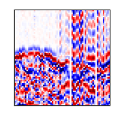
(a) Gather

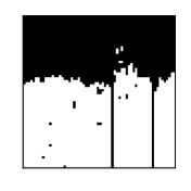
(b) UNet LT#1

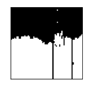
(c) STUNet

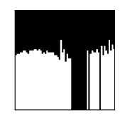
(d) GT #1

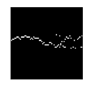
(e) UNet LT#0

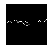
(f) UNet-D

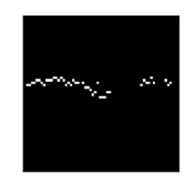
(g) Ours

(h) GT #0

Figure 5: The hot map of input gather, segmentation maps of each method, and the ground-truth images.

Moreover, we can visualize the results and analyze them more directly. Intuitively, we observe the outputs of each method, i.e., the segmentation maps, as shown in Fig. 5. In Fig. 5a, the selected input gather contains both the high SNR region (left part) and the low SNR region (right part). For current picking methods based on deep learning, it is not difficult to pick high SNR regions. However, in the low SNR regions, the result of the algorithm picking is not stable. In the face of this instability, we hope that the results of the automatic picking method would rather pick a small amount, but also ensure its accuracy. Next, we will analyze the performance of different methods under different labeling methods from the visualization results. Certainly, the pre-post FB labeling method is suggested to be used in the FB picking task training to reduce the imbalance of segmentation categories and help network optimization convergence[44]. For the pre-post FB labeling method, we empirically train UNet with LMO and STUNet picking methods, and the segmentation maps are shown in Fig. 5b and Fig. 5c, respectively. Although the general shapes of the segmentation maps (Fig. 5b and Fig. 5c) are consistent with the ground-truth (GT) map(Fig. 5d), the segmentation boundary is fuzzy, i.e., the cut-off point between 0 and 1 is not the first arrival time. Especially in the low SNR region, the incorrect FB picking is not justified. In the FB or non-FB labeling method (Fig. 5h), all methods in the high SNR area can pick the accurate first break times, but in the case of low SNR, the picking characteristics of each method are different. Concretely, the general UNet method identifies waveforms as much as possible, so that deeper waveforms are also detected shown in Fig. 5e. Using dropout in the training phase (UNet w dropout) does reduce the risk of overfitting, and Fig. 5f has a more accurate picking compared with Fig. 5e. The segmentation map of our proposed method (Fig. 5g) eliminates the picking of some regions with large variances to ensure the accuracy of the picking content.

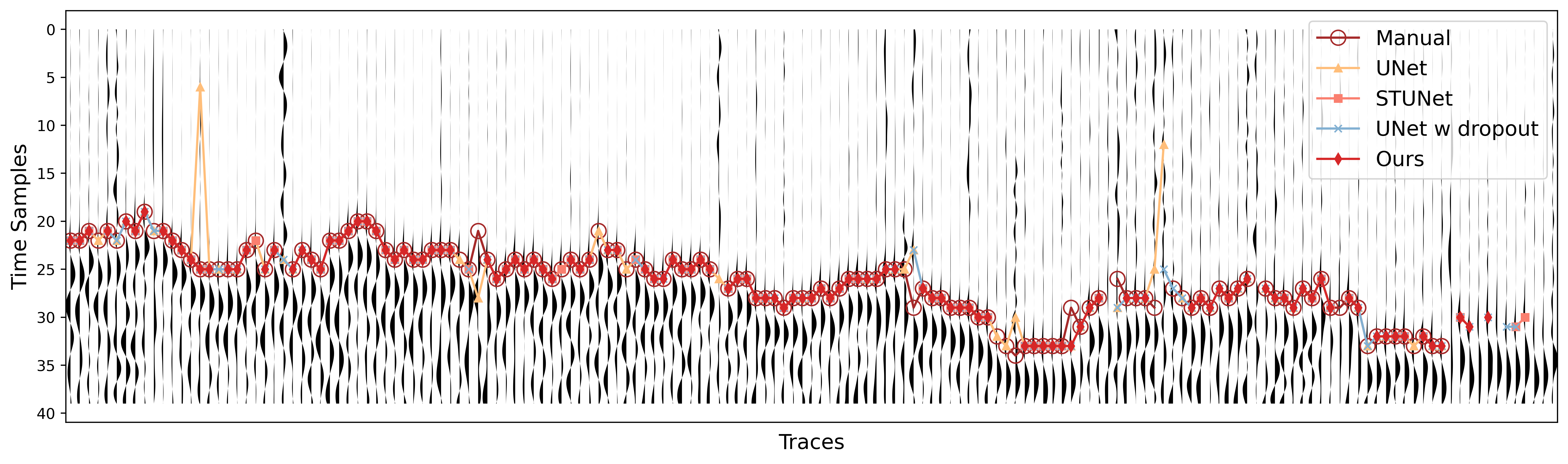
(a) Case #1

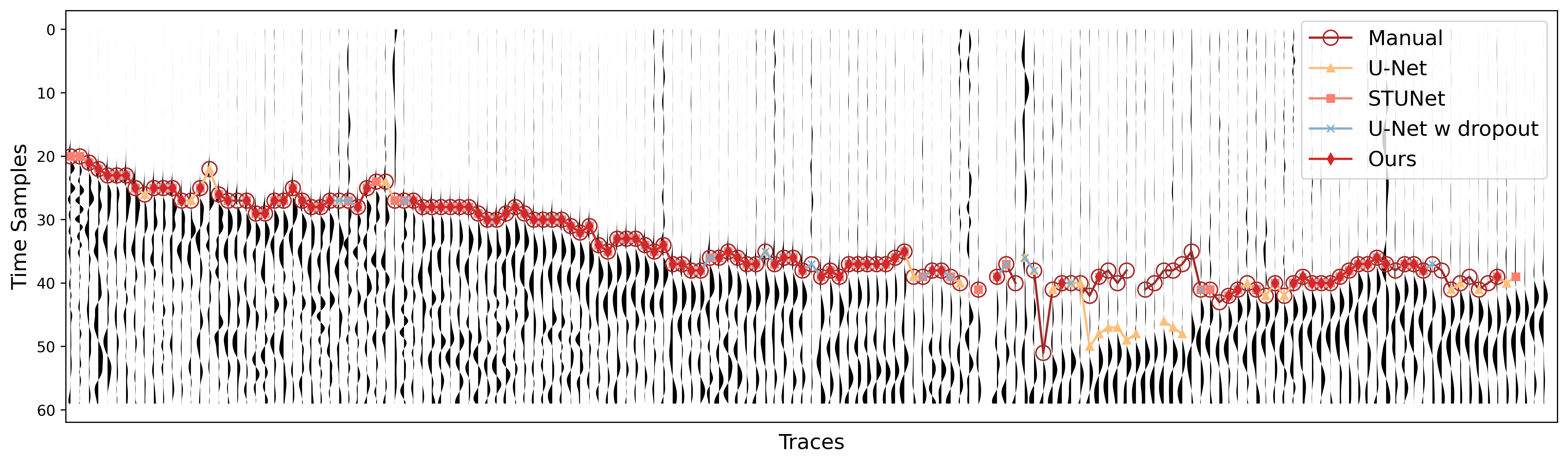
(b) Case #2

Figure 6:

Fig. 6 showcases four classical wiggle plots labeled the picking results of each method and the manual picking results. In order to better display the picking results, we only show part of the methods.

IV-D Uncertainty Representation in First Break Picking

After comparing the advantages of our method and other segmentation-based methods in evaluating metrics, we further explore why the introduction of uncertainty measures can improve the accuracy and stability of the first break picking. First of all, we give the segmentation map, variance map, and entropy map at the pixel-wise level for Bayesian U-Net. As can be seen from Fig. X, there are high variance and entropy values at the edge of the segmentation area, and high uncertainty at the incorrect first break position, which is conducive to eliminating these abnormal segmentation areas.

IV-E Robustness Test

To further test the robustness of the algorithm, we consider using the trained model to directly pick the new shot gather with different SNRs and evaluate the model with the stability and accuracy of the picking results. Concretely, the selected model is trained in the cross-survey situation to ensure that the samples predicted are from different surveys and never appear in the training set. To compare our method, we will test the UNet-based picking method with FB or non-FB labeling type[27] on the same samples with noises. In addition, Bayesian UNet and UNet models are already trained models, without any parameter adjustment in the test.

Next, we will introduce the generated shot gather with the constant SNRs. To better close the field data, we conduct injecting quantified Gaussian noise into the high SNR shot gathers which are selected manually. In this paper, we select 100 shot gathers as the high SNR dataset. The most direct way to add noise is to inject the Gaussian noise with the fixed SNR noise, where the SNR is defined by:

$$\text{SNR}=10\times\log_{10}{\frac{\sigma_{s}^{2}}{\sigma_{n}^{2}}}$$ (24)

where $\sigma_{s}^{2}$ and $\sigma_{n}^{2}$ are the variances of the trace signal and Gaussian noise, respectively. We assume that the selected high SNR set is pure. Thus, the variance of added Gaussian noise can be computed by:

$$\sigma_{n}^{2}=\sigma_{s}^{2}/10^{\text{SNR}^{*}/10}$$ (25)

where $\text{SNR}^{*}$ is the constant SNR and $\sigma_{s}^{2}$ can be estimated from each single trace signal directly.

Specifically, we generate ten data sets with Gaussian noise, whose SNRs are 5, 2, 1, -1, -3, -5, -7, -8, -9, and -10, respectively. Since different splitting thresholds greatly affect the APR and ACC, we pick FB times with many splitting thresholds and calculate the corresponding ACC and MAE of predicted results.

IV-F Ablation Study

To look deep into the Bayesian U-Net, we perform a series of ablation studies on the Halfmile dataset. Note that if not specified in all ablations the hyperparameters of training are consistent with Tab. III, and we repeat each ablation ten times with the same group of ten random seeds. We also split the Halfmile dataset into three parts: the training set, the validation set, and the test set by the ratio of 0.6: 0.2: 0.2. Each trained Bayesian U-Net picks the arrival times of the samples in the test set with sampling times = 10 or 50, and we select two metrics, i.e., MAE and Accuracy, to evaluate models.

First, the dropout layer is learned through testing models #1 and #2 in Tab. V. We only set the dropout layer in the encoder and decoder to study whether a few dropout layers can induce better performance. Test results in Tab. V show that keeping all dropout layers we select outperforms setting partial dropout layers. Second, we study whether use the transpose convolution or bilinear upsampling in the up-sample block of Bayesian U-Net. Compared with model #3 in Tab. V, our #9 surpasses a lot in all metrics. Third, we learn the effect of each input feature. Concretely, we remove one or two feature maps as the settings of the models #4, #5, and #6. Results indicate that properly increasing the number of useful feature maps can improve the performance of the Bayesian U-Net. Fourth, we also evaluate the post-processing by removing the post-processing in the test processing, i.e., the picking result based on the mean segmentation map as the final picking. Test results of Model #7 and #9 show that the post-processing based on the uncertainty qualification can filter the suspect picking to extremely improve the model performance. Finally, we investigate the effect of the forms of labels (ground truth) on model performance. Our model uses the FB or non-FB labeling method, i.e., the pixel corresponding to FB location labeled 1 and others labeled 0. There is another label method pre- or post-FB labeling method, i.e., the pixels before the FB location labeled 0 and the pixels after the FB location labeled 1. After empirical experiments (Models #8 and #9), we argue that the decision boundaries of the pre or post-FB labeling method are fuzzy and this labeling method is not suitable for very delicate pickings as shown in Fig. Based on the above studies, we evaluate the effects of the main components of the Bayesian U-Net in our method.

TABLE V: Ablation study: the test results of each ablation model

Model Num	Dropout Layer		Trans.Conv.	Post-Processing	Input Feature	Label Type	MAE (T=10)		Accuracy (T=10)		MAE (T=20)		Accuracy (T=20)
	Encoder	Decoder					Mean$\downarrow$	Std$\downarrow$	Mean$\uparrow$	Std$\downarrow$	Mean$\downarrow$	Std$\downarrow$	Mean$\uparrow$	Std$\downarrow$
#1	$\surd$		$\surd$	$\surd$	SLTA, AGC	FB or Non-FB	0.67235	1.02516	0.92979	0.06768	0.65210	1.01401	0.93122	0.06712
#2		$\surd$	$\surd$	$\surd$	SLTA, AGC	FB or Non-FB	0.27956	0.06968	0.95496	0.01578	0.26859	0.06396	0.95640	0.01537
#3	$\surd$	$\surd$		$\surd$	SLTA, AGC	FB or Non-FB	0.26014	0.08352	0.95599	0.01367	0.25618	0.08125	0.95669	0.01334
#4	$\surd$	$\surd$	$\surd$	$\surd$	None	FB or Non-FB	0.25170	0.04964	0.95800	0.00814	0.24428	0.04602	0.95893	0.00864
#5	$\surd$	$\surd$	$\surd$	$\surd$	SLTA	FB or Non-FB	0.29647	0.20094	0.95604	0.01906	0.28596	0.17643	0.95711	0.01715
#6	$\surd$	$\surd$	$\surd$	$\surd$	AGC	FB or Non-FB	0.23723	0.08308	0.96090	0.01383	0.23092	0.07995	0.96179	0.01347
#7	$\surd$	$\surd$	$\surd$		SLTA, AGC	FB or Non-FB	1.04247	2.34394	0.89374	0.18922	1.02841	2.32324	0.89480	0.18924
#8	$\surd$	$\surd$	$\surd$	$\surd$	SLTA, AGC	Pre- or Post-FB	0.49938	0.40355	0.93872	0.02537	0.41930	0.25856	0.94366	0.02172
#9 (Ours)	$\surd$	$\surd$	$\surd$	$\surd$	SLTA, AGC	FB or Non-FB	0.20257	0.03491	0.96623	0.00689	0.19885	0.04104	0.96668	0.00766

V Conclusion

In this paper, we propose a new first break time picking framework based on uncertainty qualification and semantic segmentation network, further improving the accuracy and stability of the automatic picking. The following three conclusions can be drawn from various experiments. (1) From a statistical point of view, the Bayesian U-Net can well estimate the posterior distribution of the model and infer the probability distribution of the first break times. Compared with the deterministic deep learning model, our approach is more intelligible. (2) Bayesian U-Net can be regarded as a model averaging method, so compared with a single deterministic model such as UNet, it has higher picking accuracy and stronger stability. (3) The uncertainty qualification of the first break times can reflect the confidence of the automatic picking results, and then provide suggestions for the practical picking work. (4) The proposed post-processing method based on uncertainty qualification can effectively remove error pickups to further improve the robustness of the algorithm.

Appendix A Training setting of comparative experiment

TABLE VI: Hyperparameter Selection of Comparative Experiment

Models	Training BS	Input Size	Lr	Dropout rate	Label Type
UNet LMO[27]	64	256$\times$128	1e-3	-	FB-Non FB
STUNet[32]	256	256$\times$256	1e-6	-	Pre-post FB
UNet w dropout	32	128$\times$64	1e-2	0.3	FB-Non FB

References

- [1] Ö. Yilmaz, Seismic data analysis: Processing, inversion, and interpretation of seismic data. Society of exploration geophysicists, 2001.
- [2] R. V. Allen, “Automatic earthquake recognition and timing from single traces,” Bulletin of the seismological society of America, vol. 68, no. 5, pp. 1521–1532, 1978.
- [3] M. Baer and U. Kradolfer, “An automatic phase picker for local and teleseismic events,” Bulletin of the Seismological Society of America, vol. 77, no. 4, pp. 1437–1445, 1987.
- [4] J. I. Sabbione and D. Velis, “Automatic first-breaks picking: New strategies and algorithms,” Geophysics, vol. 75, no. 4, pp. V67–V76, 2010.
- [5] S. Gaci, “The use of wavelet-based denoising techniques to enhance the first-arrival picking on seismic traces,” IEEE Transactions on Geoscience and Remote Sensing, vol. 52, no. 8, pp. 4558–4563, 2013.
- [6] S. Yung and L. T. Ikelle, “An example of seismic time picking by third-order bicoherence,” Geophysics, vol. 62, no. 6, pp. 1947–1952, 1997.
- [7] C. Saragiotis, L. Hadjileontiadis, I. Rekanos, and S. Panas, “Automatic p phase picking using maximum kurtosis and /spl kappa/-statistics criteria,” IEEE Geoscience and Remote Sensing Letters, vol. 1, no. 3, pp. 147–151, 2004.
- [8] J. B. Molyneux and D. R. Schmitt, “First-break timing; arrival onset times by direct correlation,” Geophysics, vol. 64, no. 5, pp. 1492–1501, 1999.
- [9] D. Raymer, J. Rutledge, and P. Jaques, “Semiautomated relative picking of microseismic events,” in 2008 SEG Annual Meeting. OnePetro, 2008.
- [10] J. D. Irving, M. D. Knoll, and R. J. Knight, “Improving crosshole radar velocity tomograms: A new approach to incorporating high-angle traveltime data,” Geophysics, vol. 72, no. 4, pp. J31–J41, 2007.
- [11] K. De Meersman, J.-M. Kendall, and M. Van der Baan, “The 1998 valhall microseismic data set: An integrated study of relocated sources, seismic multiplets, and s-wave splitting,” Geophysics, vol. 74, no. 5, pp. B183–B195, 2009.
- [12] D. Kim, Y. Joo, and J. Byun, “First-break picking method based on the difference between multi-window energy ratios,” IEEE Transactions on Geoscience and Remote Sensing, 2023.
- [13] Y. Xu, C. Yin, X. Zou, Y. Ni, Y. Pan, and L. Xu, “A high accurate automated first-break picking method for seismic records from high-density acquisition in areas with a complex surface,” Geophysical Prospecting, vol. 68, no. 4, pp. 1228–1252, 2020.
- [14] L. Gao, H. Jiang, and F. Min, “Stable first-arrival picking through adaptive threshold determination and spatial constraint clustering,” Expert Systems with Applications, vol. 182, p. 115216, 2021.
- [15] Z. Lan, P. Gao, P. Wang, Y. Wang, J. Liang, and G. Hu, “Automatic first arrival time identification using fuzzy c-means and aic,” IEEE Transactions on Geoscience and Remote Sensing, vol. 60, pp. 1–13, 2021.
- [16] M. D. McCormack, D. E. Zaucha, and D. W. Dushek, “First-break refraction event picking and seismic data trace editing using neural networks,” Geophysics, vol. 58, no. 1, pp. 67–78, 1993.
- [17] S. Yuan, J. Liu, S. Wang, T. Wang, and P. Shi, “Seismic waveform classification and first-break picking using convolution neural networks,” IEEE Geoscience and Remote Sensing Letters, vol. 15, no. 2, pp. 272–276, 2018.
- [18] X. Duan and J. Zhang, “Multitrace first-break picking using an integrated seismic and machine learning method,” Geophysics, vol. 85, no. 4, pp. WA269–WA277, 2020.
- [19] C. Guo, T. Zhu, Y. Gao, S. Wu, and J. Sun, “Aenet: Automatic picking of p-wave first arrivals using deep learning,” IEEE Transactions on Geoscience and Remote Sensing, vol. 59, no. 6, pp. 5293–5303, 2020.
- [20] X. Duan and J. Zhang, “Multi-trace and multi-attribute analysis for first-break picking with the support vector machine,” in SEG Technical Program Expanded Abstracts 2019. Society of Exploration Geophysicists, 2019, pp. 2559–2563.
- [21] M. Mkezyk and M. Malinowski, “Multi-pattern algorithm for first-break picking employing open-source machine learning libraries,” Journal of Applied Geophysics, vol. 170, p. 103848, 2019.
- [22] J. Long, E. Shelhamer, and T. Darrell, “Fully convolutional networks for semantic segmentation,” in Proceedings of the IEEE conference on computer vision and pattern recognition, 2015, pp. 3431–3440.
- [23] O. Ronneberger, P. Fischer, and T. Brox, “U-net: Convolutional networks for biomedical image segmentation,” in Medical Image Computing and Computer-Assisted Intervention–MICCAI 2015: 18th International Conference, Munich, Germany, October 5-9, 2015, Proceedings, Part III 18. Springer, 2015, pp. 234–241.
- [24] K. C. Tsai, W. Hu, X. Wu, J. Chen, and Z. Han, “First-break automatic picking with deep semisupervised learning neural network,” in SEG Technical Program Expanded Abstracts 2018. Society of Exploration Geophysicists, 2018, pp. 2181–2185.
- [25] ——, “Automatic first arrival picking via deep learning with human interactive learning,” IEEE Transactions on Geoscience and Remote Sensing, vol. 58, no. 2, pp. 1380–1391, 2019.
- [26] T. Xie, Y. Zhao, X. Jiao, W. Sang, and S. Yuan, “First-break automatic picking with fully convolutional networks and transfer learning,” in SEG International Exposition and Annual Meeting. OnePetro, 2019.
- [27] L. Hu, X. Zheng, Y. Duan, X. Yan, Y. Hu, and X. Zhang, “First-arrival picking with a u-net convolutional networkfirst-arrival picking with u-net,” Geophysics, vol. 84, no. 6, pp. U45–U57, 2019.
- [28] Y. Ma, S. Cao, J. W. Rector, and Z. Zhang, “Automatic first arrival picking for borehole seismic data using a pixel-level network,” in SEG International Exposition and Annual Meeting. OnePetro, 2019.
- [29] S.-C. Pierre-Luc, R. Bruno, G. Joumana, N. Jean-Philippe, B. Gilles, and S. Ernst, “A multi-survey dataset and benchmark for first break picking in hard rock seismic exploration,” in Proc. Neurips 2021 Workshop on Machine Learning for the Physical Sciences (ML4PS), 2021.
- [30] S. Han, Y. Liu, Y. Li, and Y. Luo, “First arrival traveltime picking through 3-d u-net,” IEEE Geoscience and Remote Sensing Letters, vol. 19, pp. 1–5, 2021.
- [31] P. Yuan, S. Wang, W. Hu, X. Wu, J. Chen, and H. Van Nguyen, “A robust first-arrival picking workflow using convolutional and recurrent neural networks,” Geophysics, vol. 85, no. 5, pp. U109–U119, 2020.
- [32] P. Jiang, F. Deng, X. Wang, P. Shuai, W. Luo, and Y. Tang, “Seismic first break picking through swin transformer feature extraction,” IEEE Geoscience and Remote Sensing Letters, vol. 20, pp. 1–5, 2023.
- [33] Y. LeCun, Y. Bengio, and G. Hinton, “Deep learning,” nature, vol. 521, no. 7553, pp. 436–444, 2015.
- [34] M. Abdar, F. Pourpanah, S. Hussain, D. Rezazadegan, L. Liu, M. Ghavamzadeh, P. Fieguth, X. Cao, A. Khosravi, U. R. Acharya et al., “A review of uncertainty quantification in deep learning: Techniques, applications and challenges,” Information Fusion, vol. 76, pp. 243–297, 2021.
- [35] Y. Gal and Z. Ghahramani, “Dropout as a bayesian approximation: Representing model uncertainty in deep learning,” in international conference on machine learning. PMLR, 2016, pp. 1050–1059.
- [36] C. Blundell, J. Cornebise, K. Kavukcuoglu, and D. Wierstra, “Weight uncertainty in neural network,” in International conference on machine learning. PMLR, 2015, pp. 1613–1622.
- [37] B. Lakshminarayanan, A. Pritzel, and C. Blundell, “Simple and scalable predictive uncertainty estimation using deep ensembles,” Advances in neural information processing systems, vol. 30, 2017.
- [38] A. Kendall, V. Badrinarayanan, and R. Cipolla, “Bayesian segnet: Model uncertainty in deep convolutional encoder-decoder architectures for scene understanding,” arXiv preprint arXiv:1511.02680, 2015.
- [39] S. Sankaran, L. Grady, and C. A. Taylor, “Fast computation of hemodynamic sensitivity to lumen segmentation uncertainty,” IEEE transactions on medical imaging, vol. 34, no. 12, pp. 2562–2571, 2015.
- [40] A. Mehrtash, W. M. Wells, C. M. Tempany, P. Abolmaesumi, and T. Kapur, “Confidence calibration and predictive uncertainty estimation for deep medical image segmentation,” IEEE transactions on medical imaging, vol. 39, no. 12, pp. 3868–3878, 2020.
- [41] M. Kampffmeyer, A.-B. Salberg, and R. Jenssen, “Semantic segmentation of small objects and modeling of uncertainty in urban remote sensing images using deep convolutional neural networks,” in Proceedings of the IEEE conference on computer vision and pattern recognition workshops, 2016, pp. 1–9.
- [42] C. W. Fox and S. J. Roberts, “A tutorial on variational bayesian inference,” Artificial intelligence review, vol. 38, pp. 85–95, 2012.
- [43] T.-Y. Lin, P. Goyal, R. Girshick, K. He, and P. Dollár, “Focal loss for dense object detection,” in Proceedings of the IEEE international conference on computer vision, 2017, pp. 2980–2988.
- [44] S.-Y. Yuan, Y. Zhao, T. Xie, J. Qi, and S.-X. Wang, “Segnet-based first-break picking via seismic waveform classification directly from shot gathers with sparsely distributed traces,” Petroleum Science, vol. 19, no. 1, pp. 162–179, 2022.