The interaction between two close-to-touching convex acoustic subwavelength resonators
Abstract.
The Minneart resonance is a low frequency resonance in which the wavelength is much larger than the size of the resonators. It is interesting to study the interaction between two adjacent bubbles when they are brought close together. Because the bubbles are usually compressible, in this paper we mainly investigate resonant modes of two general convex resonators with arbitrary shapes to extend the results of Ammari, Davies, Yu in [4], where a pair of spherical resonators are considered by using bispherical coordinates. We combine the layer potential method for Helmholtz equation in [4, 5] and the elliptic theory for gradient estimates in [26, 30] to calculate the capacitance coefficients for the coupled resonators, then show the leading-order asymptotic behaviors of two different resonant modes and reveal the dependance of the resonant frequencies on their geometric properties, such as convexity, volumes and curvatures. By the way, the blow-up rates of gradient of the scattered pressure are also presented.
1. Introduction, Formulation and Main Results
1.1. Background
In recent years, the acoustic properties and applications of bubbly media were investigated in various aspects, since it was discovered that a very small volume fraction of air bubbles in water is enough to modify the effective velocity of sound in the medium, see Minnaert’s well-known work [33] and [7, 17]. The enhancement of their acoustic signature allows ultrasonic techniques to detect, localize, and characterize them inside a visco-elastic opaque medium [16]. The extraordinary acoustic properties of bubbly media are also used to design new acoustic materials, because the Minnaert resonance of the bubbles persists not only in liquid but also in the soft elastic medium, where the resonators are commonly constructed from a material that has greatly different material parameters to the background medium. There are many interesting works in physics as well on the acoustic bubble problem, see [31] and the references therein. In practice, structures made from subwavelength resonators (a type of metamaterial) also have been used for a wide variety of wave-guiding applications, e.g. [8, 25, 5, 2, 3].
The Minnaert resonance is a low frequency resonance in which the wavelength is much larger than the size of the bubbles [17]. It is very interesting to study the interaction between two adjacent bubbles when they are brought close together. Using to express the distance between them, Ammari, Davies, Yu [4] recently studied the behavior of the coupled subwavelength resonant modes of a pair of spherical resonators. They employed the layer potential method to represent solutions and proved that the leading-order behavior of the resonant modes is determined by the so-called capacitance coefficients [8], which are well known in the setting of electrostatics, and then calculated them by using bispherical coordinates. However, considering that the bubbles are usually compressible and not necessarily spherical, and in view of shape optimization for applications, it is necessary and important to study the resonators with arbitrary shapes. Motivated by [4], in this paper we mainly deal with the case of general convex resonators in order to explore more applications of subwavelength resonant media.
This multi-scale problem involves the high contrast parameter, , of the material density, the small separation distance, , between the two resonators, the volume and local curvatures of each resonator. From the technical point of view, the technique in this paper breaks the restriction to spheres due to the use of bi-spherical coordinates on the circular case, which allows us to distinguish the effect from the volume (global information) and curvatures (local information) on the resonant frequencies. On the other hand, it can be applied to deal with ellipsoidal resonators, -convex resonators, and even more general convex resonators of arbitrary shape. The main result of this paper shows that both two sub-wavelength resonant frequencies as with chosen to be a suitable function of , and their asymptotic behaviors are of different scales when the distance between the resonators is sufficiently small (see Theorem 1.8 and Remark 1.11 for more details).
We first use the layer potential method to perform an asymptotic analysis in terms of the material contrast [7, 8], examine the behavior of the eigenmodes when the resonators are brought together [4], and reduce the leading order behavior of the resonant modes to the calculation of the so-called capacitance coefficients. Then, we adapt the local gradient estimates for the Laplace equation developed in [26, 29] to compute asymptotic expansions of the capacitance coefficients for the resonators with -convex boundaries, , in the exterior domain. Compared with [26, 30], the difference here is that the domain we consider in this paper is unbounded while it is bounded in [26, 30]. Especially, we need to control the asymptotic behavior at infinity and extend the results in bounded domains to unbounded domains. Finally, similarly as in [4], we show that there are two subwavelength resonant frequencies (see Lemma 1.4 below) having different asymptotic behaviors and depending on the contrast of the density, the convexity, volumes, curvatures of the resonators, which can be neatly expressed when the separation distance is chosen as a function of the material contrast. This may have significant implications for the design of acoustic meta-materials with multi-frequency or broadband functionality. As a consequence, we show the dependence of the blow-up rate of the gradient on the geometry of the resonators, is similar to electrostatics [9, 23, 12, 32, 35] and linear elasticity [22, 13, 14, 27] and the references therein, provided the parameters of the inclusions degenerate to infinity. Here we remark that our method is different from the method used in [4] where the authors use bi-spherical coordinates to derive explicit representations for the capacitance coefficients and capture the system’s resonant behavior at leading order. Finally, we would like to point out that in this present paper and [4] the material parameters are positive, which are different from the surface plasmons studied in [34, 15, 24], where the electromagnetic inclusions have negative permittivities.
1.2. Helmholtz Equations
In this paper, we study the scattering problem in dimension three of the Helmholtz equation in a high-contrast composite structure, especially when the inclusions are closely spaced. Assume that in a homogeneous background medium, with density and bulk modulus , there is a pair of convex resonators and -apart, for a small constant . Let and denote the density and bulk modulus of the medium that occupies . In this paper we assume that and are of arbitrary shape, with boundaries, . We follow the notations in [4] and introduce the auxiliary parameters
| (1.1) |
which are the wave’s speeds and wave’s numbers in and in , respectively, and two dimensionless contrast parameters
Then the acoustic pressure produced by the scattering of an incoming plane wave satisfies
| (1.2) |
along with the Sommerfeld radiation condition:
where the subscripts and denote the evaluation from outside and inside , respectively. We assume that , , are all , while the contrast of the density . A classic example satisfying these assumptions is a collection of air bubbles in water, often known as Minnaert bubbles, in which case .
1.3. Our Domains
Before stating the main results we first describe our domains precisely. We use to denote a point in , where . Let and be a pair of touching convex subdomains in , such that
| (1.3) |
with being their common tangent plane, and . We further assume that the norms of are bounded by some constants to guarantee that their volumes are independent of (or of a scale of different order compared to ). Translating by along the -axis, we have . When there is no confusion, we always drop the superscripts, and denote
and
We remark that here our domains and are both unbounded, different from the case of bounded domain considered previously in [26, 30].
Near the origin, similarly as in [13, 26], let us set the two boundary points
By our smoothness assumptions, there exists a small universal constant such that the portions of near can be parameterized by and , respectively, namely,
By the convexity assumptions on , and satisfy
| (1.4) |
| (1.5) |
and
| (1.6) |
For simplicity, we assume that
| (1.7) | ||||
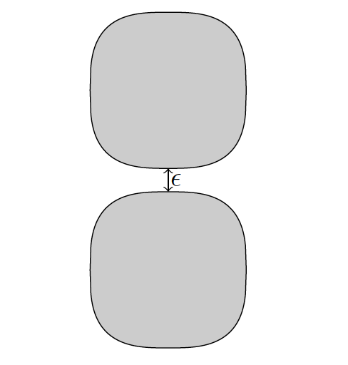
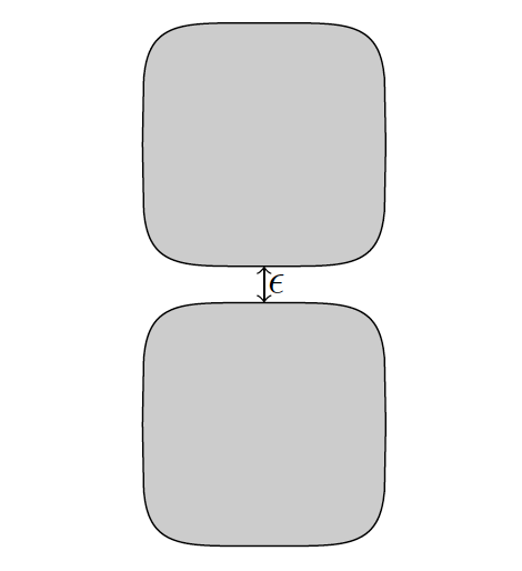
and is an integer, . Here and throughout the paper, we use the notation to denote a quantity that can be bounded by , where is some positive constant independent of and . We call such inclusions -convex inclusions. For example, there is a curvilinear square with rounded-off angles, with boundary given by
for some positive , representing a half width of the inclusion, see Figure 2 and Figure 2. We would like to point out that in dimension two this type of inclusion is very close to the Vigdergauz inclusion (see Fig. 3 in [28]), which has also a nearly square shape and is proved to minimize the elastic energy under the same volume fraction of hard inclusions [19]. More discussions on the connection between -convex inclusion and the Vigdergauz inclusion can refer to page 7-8 in [28]. So it is interesting to consider -convex inclusion and use the simple curve boundary (1.7) to describe narrow region between two inclusions with nearly square shapes. This is also one motivation of this paper.
For more general domains, see Remark 1.12 below. Here and throughout this paper, unless otherwise stated, denotes a constant, whose values may vary from line to line, depending only on , and , not on . We call a constant having such dependence a universal constant.
1.4. Layer Potential for the Helmholtz Equations
In this subsection, we follow the definitions and the notations used in [4]. More properties on the layer potential theory and the Neumann–Poincaré operator can be found in [6]. For the Helmholtz equation
let be the (outgoing) Helmholtz Green’s function
and be the corresponding single layer potential, see [10], defined by
Here is the usual Sobolev space. We also define the Neumann–Poincaré operator by
where denotes the outward normal derivative at . By recalling the transmission conditions for the single layer potential on [6], in particular, for any ,
| (1.8) |
Using the exponential power series we can derive an expansion for , given by
| (1.9) |
where, for ,
and is the Laplace single layer potential. It is well known that is invertible [6]. Similarly, for we have that
| (1.10) |
where, for ,
and is the Neumann–Poincaré operator corresponding to the Laplace equation. In fact, by the following Lemma, as we could write and in the relevant operator norms respectively .
Lemma 1.1.
The solutions to (1.2) can be represented as follows:
| (1.11) |
for some surface potentials , which must be chosen so that satisfies the two transmission conditions across . Using the jump relation (1.8), this is equivalent to satisfying
| (1.12) |
where
| (1.13) |
and is the identity operator on , see e.g. [6] for more details.
1.5. Resonant Frequencies and the Capacitance Coefficients
In light of the representation (1.11), we can define the notion of resonance to be the existence of a non-trivial solution when the incoming field is zero.
Definition 1.2.
For a fixed , we define a resonant frequency (or eigenfrequency) to be such that there exists a non-trivial solution to
where is defined in (1.13). For each resonant frequency , we define the corresponding resonant mode (or eigenmode) as
| (1.14) |
Definition 1.3.
We define a subwavelength resonant frequency to be a resonant frequency such that , and depends on continuously.
The resonant modes (1.14) are determined only up to normalization. We will choose the normalization to be such that on for all small and , see Theorem 4.1 below. When and ,
| (1.15) |
Since is invertible, it follows that . By the argument in Lemma 2.12 of [2], we know that
Notice that each resonant mode in fact has two resonant frequencies associated to it with real parts that differ in sign. Here, we use to denote the resonant frequency associated to that has a positive real part. By virtue of Lemma 1.6 below, is also a resonant frequency associated to the mode . See Lemma 1.4 and Remark 1.7 below.
Lemma 1.4.
([4]) There exist two subwavelength resonant modes, and , with associated resonant frequencies and with positive real part, labelled such that .
Now let be given by
| (1.16) |
It follows that
| (1.17) |
Let be defined as the extension of (1.16) to . Then is the unique solution to
| (1.18) |
We define the capacitance matrix as follows:
| (1.19) |
Thanks to the jump relation (1.8) and the fact that satisfies the (1.17),
Thus, we can write the capacitance coefficients in the form
| (1.20) |
For , by applying the divergence theorem, and in view of Proposition 2.74 and 2.75 in [18], which imply that as , we have
| (1.21) |
Denote
| (1.22) |
and
| (1.23) |
Then, we adapt the method in [26] for gradient estimates for the Dirichlet problem in bounded domain to exterior domains and obtain the following asymptotic formula for the capacitance coefficients.
Proposition 1.5.
(i) there exist constants , depending only on and , such that
| (1.24) |
(ii) there exists a constant , independent of , such that
| (1.25) |
Denote the rescaled form of by
| (1.26) |
where denotes the volume of . Let denote the eigenvalues of matrix . A simple calculation yields
| (1.27) |
Then the resonant frequencies are determined by and . The following relationship is from Lemma 4.1 in [4], which actually holds for bounded domains with Lipschitz boundaries, see Lemma 2.1 of [8]. For the reader’s convenience, we give some details of the proof.
Lemma 1.6.
Proof.
The proof is the same as that of Lemma 4.1 of [4]. Suppose that is a solution to (1.2) for small . From (1.2) and the asymptotic expansions (1.9) and (1.10), we have
| (1.28) |
Therefore,
| (1.29) |
Since is invertible [6], and by virtue of Lemma 1.1, is bounded, it follows that in . Now by virtue of Lemma 2.1 of [8] (where the boundary is assumed to be Lipschitz), we have, for any
| (1.30) |
Using (1.28) again, we get
| (1.31) |
Integrating (1.31) over , using (1.30) yields
| (1.32) |
Remark 1.7.
By (1.35), we know that is the eigenvalue of , up to an error of order , , so we have . We use to denote the resonant frequency that has a positive real part, which means that we write as . Here we would like to point out that in fact the resonant frequencies and are not real-valued, their imaginary parts will appear in the term. Because we are studying resonators in an unbounded domain, energy is lost to the far field meaning that the resonant frequencies have negative imaginary parts [2, 7, 8]. Hence, the leading-order terms in the expansions for and (given in Lemma 1.6) are real valued and the imaginary parts will appear in higher-order terms in the expansion. However, by Lemma 1.1 only the leading-order terms in the asymptotic expansion (1.9) and (1.10) have singularities as the resonators are moved close together, we do not consider the higher-order expansions in this work.
1.6. Main Results
Setting
| (1.36) |
by using (1.25), we have
| (1.37) |
Furthermore, let
| (1.38) |
Thus, by virtue of (1.37) and (1.25), there exists some constant , independent of , such that
| (1.39) |
Thanks to the explicit calculation of the capacitance coefficients in Proposition 1.5 and the relation between the subwavelength resonant frequencies and the capacitance proved in the Lemma 1.6, we could compute the asymptotic expansions of the subwavelength resonant frequencies in terms of and as . Now we state our main result as follows. It is valid for the convex resonators of arbitrary shape.
Theorem 1.8.
Remark 1.9.
Consequently, since , it follows from (1.40) that the corresponding wavenumber satisfying
Remark 1.10.
If we choose as an appropiate function of , then we can obtain the asymptotic behavior of . For example, if we choose for ; while for , where , then we have , and .
Proof of Theorem 1.8.
Remark 1.11.
Remark 1.12.
The rest of this paper is organized as follows. We first give some preliminary results for the Dirichlet problem of the Laplace equation in an exterior domain and then extend the gradient estimates result in [26, 30] to exterior domains in Section 2. In Section 3, we mainly prove Proposition 1.5. Finally, we present the corresponding gradient blow-up results in Section 4.
2. Preliminaries
This section is devoted to proving some basic results for the problem in the exterior domains or . For simplicity, we assume that
Lemma 2.1.
Suppose is a solution of (1.18). Then in .
Proof.
Fix . By virtue of the fact that as , then for any , we can choose sufficiently large , such that . Because
then, by using the maximum principle in the region , we have . Because and are arbitrary, the proof is finished. ∎
Lemma 2.2.
Suppose is a solution of (1.18). Then for sufficiently large , such that , we have
| (2.1) |
where the Poison kernel , , is the fundamental solution of the Laplace equation in dimension three, and . Moreover, the following derivative estimates hold when ,
| (2.2) |
Proof.
For , let
To prove Propostion 1.5, we introduce the Keller-type function , as in [26, 13] for instance, such that on , on , and as , especially,
| (2.3) |
where , and satisfies
| (2.4) |
In view of (2.3), a direct calculation gives
| (2.5) |
Although is defined in an unbounded domain in this paper, the same result as Proposition 1.7 in [26] holds.
Lemma 2.3.
Suppose is a solution of (1.18). Then
| (2.6) |
Proof.
An immediate consequence of Lemma 2.3 is as follows.
Corollary 2.4.
In order to investigate the asymptotic expansions of , we need to consider the following limit problem
| (2.9) |
Similarly as lemma 3.1 in [12], we have
Lemma 2.5.
There exists a unique solution to (2.9).
Proof.
It is easy to find a subharmonic function in , such that at infinity and satisfying the boundary condition . Then, the existence of solution can be easily obtained by the Perron method, see theorem 2.12 and lemma 2.13 in [20]. The regularity for follows from the standard elliptic theory, due to the fact that the boundary of the domain is except the origin, see e.g. Theorem 10.2 in [11]. ∎
For , let
Similarly as , we construct , such that , as , on , on ,
| (2.10) |
and . It is easy to see that
| (2.11) |
It follows from the Proof of Lemma 2.3 that
This implies that is also the main term of .
Proof.
Since it is obvious that on , and as , we only need to estimate the values of on and at infinity. We divide into two parts: (a) and (b) .
3. Proof of Proposition 1.5
This section is devoted to proving Proposition 1.5. We prove part (i) and part (ii) in Subsection 3.1 and Subsection 3.2, respectively. Here the asymptotic behavior at infinity is mainly dealt with.
3.1. Proof of (i) in Proposition 1.5
Let
Then
Lemma 3.1.
For sufficiently small , we have , moreover,
| (3.1) |
Proof.
Proof of (i) in Proposition 1.5 .
To prove (i) in Proposition 1.5, we first divide the integral into two parts:
| (3.2) |
where , , and we take , for convenience.
STEP 1. First, we use the explicit functions and to approximate in the unbounded region and the small region , respectively. We claim that
| (3.3) |
where is defined by (1.22).
Indeed, we further divide into two parts:
| (3.4) | ||||
For , we rearrange it as follows:
By virtue of Lemma 3.1, we have
Since
and
it follows by standard elliptic regularity theory that
where is independent of , provided , are .
By interpolation inequalities, see e.g. Lemma 6.32 and Lemma 6.35 in [20], for , , we have
Taking , by using the interpolation above with (2.12), we have
So, . In view of the boundedness of in and , and their volumes and are less than , it is easy to get . Hence, .
STEP 2. Next we prove that
where
Indeed, similarly as Lemma 2.2, we have , and . Combining with in , and the divergence theorem, we obtain . For , using ,
we have , and
On the other hand, recalling (2.5), we have
here we used
While, it follows from (2.11) and (2.5) that
| (3.6) |
Thus, to prove (1.24), it suffices to calculate the integral in the right hand side of (3.1).
STEP 3. We now calculate the integral in (3.1).
For ,
where . Therefore, (1.24) holds with . Finally, we show that the constant is independent of the choice of . If not, suppose that there exist and , both independent of , such that (1.24) holds, then
which implies that . For , the proof is the same. Thus, the proof of (i) in Proposition 1.5 is completed. ∎
3.2. Proof of (ii) in Proposition 1.5
Lemma 3.2.
, where is defined as (1.26).
Proof.
For any large , By appying the divergence theorem, we have
Using as , and Proposition 2.74 and 2.75 in [18], which imply that as , and due to the arbitrariness of , we finish the proof. ∎
Proof of (ii) in Proposition 1.5.
By using Lemma 3.2, and applying the divergence theorem on , such that , we have
| (3.8) |
Recalling the Poisson formula, (2.1),
where is fixed in (2.1). Now , , since in , we choose , such that
By using 3.1,
Integrating on , by (3.8), yields
The proof for is similar. So the proof of Proposition 1.5 is completed. ∎
4. Gradient Blow-up
It is known the eigenmode is approximately a constant on each resonator. If these constants are different, then as the two resonators are moved close together, the gradient of the field between them will blow up. As a direct consequence of Theorem 1.8, we can also show the gradient blow-up of the eigenmode similarly as in [4].
As in (1.27), the eigenvector of associated to the eigenvalue is given by
| (4.1) |
From the leading order behaviour of , (1.6), and of the capacitance coefficients (1.26) we have that, for ,
| (4.2) |
Then the eigenmodes are given by
| (4.3) |
By using (1.33) in Lemma 1.6, we have
| (4.4) |
Note that . Then
| (4.5) | ||||
Hence,
| (4.6) |
Therefore, for sufficiently small , and have the same sign whereas and have different signs.
Further,
| (4.7) |
Since , and , due to Lemma 2.3 of [12] (or the result in [1, 29]), we have
Thus, due to Proposition 1.5, and (1.39) in Proposition 1.5, we know that the main singular part of is .
Combining with (4.2), as a consequence of Proposition 1.5, we obtain the following gradient estimates for the two eigenmodes and similarly as in [4]. Namely, choose so that as , if the two leading order values are different then the maximum of the gradient of the presure between the two resonators must blow up as .
Theorem 4.1.
Let and denote the sub-wavelength eigenmodes for two m-convex resonators and in , which are -apart as in Theorem 1.8. Normalize and such that
Then suppose that the distance satisfies for , for , for , we have, as ,
and
Acknowledgements. We thank the referees for carefully reading and many helpful suggestions which improve the exposition.
References
- [1] H. Ammari, G. Dassios, H. Kang, and M. Lim, Estimates for the electric field in the presence of adjacent perfectly conducting spheres. Quart. Appl. Math. 65(2): 339–355, 2007.
- [2] H. Ammari; B. Davies, A fully-coupled subwavelength resonance approach to filtering auditory signals. Proc. A. 475 (2019), no. 2228, 20190049, 17 pp.
- [3] H. Ammari, B. Davies, E. O. Hiltunen, S. Yu, Topologically protected edge modes in one-dimensional chains of subwavelength resonators. J. Math. Pures Appl. (9) 144 (2020), 17-49.
- [4] H. Ammari; B. Davies; S. Yu, Close-to-touching acoustic subwavelength resonators: eigenfrequency separation and gradient blow-up. Multiscale Model. Simul. 18 (2020), no. 3, 1299-1317.
- [5] H. Ammari, B. Fitzpatrick, D. Gontier, H. Lee, and H. Zhang, subwavelength focusing of acoustic waves in bubbly media. Proc. A. 473 (2208):20170469, 2017.
- [6] H. Ammari, B. Fitzpatrick, H. Kang, M. Ruiz, S. Yu, and H. Zhang, Mathematical and Computational Methods in Photonics and Phononics, Math. Surveys Monogr. 235, AMS,Providence, RI, 2018.
- [7] H. Ammari, B. Fitzpatrick, D. Gontier, H. Lee, and H. Zhang, Minnaert resonances for acoustic waves in bubbly media. Ann. I. H. Poincaré–A. N. 35(7): 1975–1998, 2018.
- [8] H. Ammari, B. Fitzpatrick, H. Lee, S. Yu, and H. Zhang, Double-negative acoustic metamaterials. Quart. Appl. Math. 77(4):767–791, 2019.
- [9] H. Ammari; H. Kang; M. Lim, Gradient estimates to the conductivity problem. Math. Ann. 332 (2005), 277-286.
- [10] H. Ammari, H. Kang, and H. Lee, Layer Potential Techniques in Spectral Analysis, Math. Surveys Monogr. 153, AMS, Providence, RI, 2009.
- [11] S. Agmon; A. Douglis; L. Nirenberg. Estimates near the boundary for solutions of elliptic partial differential equations satisfying general boundary conditions. II. Comm. Pure Appl. Math. 17 (1964), 35-92.
- [12] E. Bao; Y.Y. Li; B. Yin, Gradient estimates for the perfect conductivity problem. Arch. Ration. Mech. Anal. 193 (2009), 195-226.
- [13] J.G. Bao, H.G. Li, and Y.Y. Li, Gradient estimates for solutions of the Lamé system with partially infinite coefficients, Arch. Ration. Mech. Anal. 215 (2015), 307-351.
- [14] J.G. Bao, H.G. Li, Y.Y. Li, Gradient estimates for solutions of the Lamé system with partially infinite coefficients in dimensions greater than two. Adv. Math. 305 (2017), 298-338.
- [15] E. Bonnetier and F. Triki. On the spectrum of the poincaré variational problem for two close-to-touching inclusions in 2d. Arch. Rational Mech. Anal. 209(2): 541–567, 2013.
- [16] D.C. Calvo, A.L. Thangawng, C.N. Layman, Low-frequency resonance of an oblate spheroidal cavity in a soft elastic medium, J. Acoust. Soc. Am. 132 (2012) EL1–EL7.
- [17] M. Devaud; T. Hocquet; J.-C. Bacri; V. Leroy, The minnaert bubble: an acoustic approach. Eur. J. Phys. 29(6):1263, 2008.
- [18] G.B. Folland, Introduction to Partial Differential Equations, Princeton University Press, Princeton, NJ, 1976.
- [19] Grabovsky, Y., Kohn, R.V.: Microstructure minimizing the energy of a two phase elastic composite in two space dimensions II. J. Mech. Phys. Solids 43, 949–972 (1995)
- [20] D. Gilbarg; N.S. Trudinger, Elliptic partial differential equations of second order, Reprint of the 1998 edition, Classics in Mathematics. Springer, Berlin, 2001.
- [21] I. Gohberg and J. Leiterer, Holomorphic Operator Functions of One Variable and Applications: Methods from Complex Analysis in Several Variables, Oper. Theory Adv. Appl.192, Birkhäuser, Basel, 2009.
- [22] H. Kang, S. Yu, Quantitative characterization of stress concentration in the presence of closely spaced hard inclusions in two-dimensional linear elasticity, Arch. Ration. Mech. Anal. 232 (2019), 121-196.
- [23] Y. Gorb. Singular behavior of electric field of high-contrast concentrated composites. Multiscale Model. Sim. 13(4):1312–1326, 2015.
- [24] H. K. Khattak, P. Bianucci, and A. D. Slepkov. Linking plasma formation in grapes to microwave resonances of aqueous dimers. P. Nat. Acad. Sci. USA 116(10):4000–4005, 2019.
- [25] M. Kushwaha, B. Djafari-Rouhani, and L. Dobrzynski. Sound isolation from cubic arrays of air bubbles in water. Phys. Lett. A 248(2-4):252–256, 1998.
- [26] H.G. Li, Asymptotics for the electric field concentration in the perfect conductivity problem. SIAM J. Math. Anal. 52 (2020), no. 4, 3350–3375.
- [27] H.G. Li, Lower bounds of gradient’s blow-up for the Lamé system with partially infinite coefficients. J. Math. Pures Appl. (9) 149 (2021), 98-134.
- [28] H.G. Li; Y. Li, An extended Flaherty-Keller formula for an elastic composite with densely packed convex inclusions. Calc. Var. Partial Differential Equations 61 (2022), no. 3, Paper No. 90, 28 pp.
- [29] H.G. Li; Y.Y. Li; E.S. Bao; B. Yin, Derivative estimates of solutions of elliptic systems in narrow regions, Quart. Appl. Math. 72 (2014), pp. 589-596.
- [30] H.G. Li; Y.Y. Li; Z.L. Yang, Asymptotics of the gradient of solutions to the perfect conductivity problem. Multiscale Model. Simul. 17 (2019), no. 3, 899–925.
- [31] M. Lanoy, R. Pierrat, F. Lemoult, M. Fink, V. Leroy, A. Tourin, subwavelength focusing in bubbly media using broadband time reversal, Phys. Rev. B 91 (22) (2015) 224202.
- [32] J. Lekner. Near approach of two conducting spheres: Enhancement of external electric field. J. Electrostat. 69(6):559–563, 2011.
- [33] M. Minnaert. On musical air-bubbles and the sounds of running water. Philos. Mag. 16(104):235–248, 1933.
- [34] S. Yu and H. Ammari. Plasmonic interaction between nanospheres. SIAM Rev. 60(2):356–385, 2018.
- [35] K. Yun, Estimates for electric fields blown up between closely adjacent conductors with arbitrary shape. SIAM J. Appl. Math. 67 (2007), 714–730.