An Optical Analog for a Rotating Binary Bose–Einstein Condensate

Abstract

Coupled nonlinear Schrödinger equations for paraxial optics with two circular polarizations of light in a defocusing Kerr medium with anomalous dispersion coincide in form with the Gross–Pitaevskii equations for a binary Bose–Einstein condensate (BEC) of cold atoms in the phase separation regime. In this case, the helical symmetry of an optical waveguide corresponds to rotation of the transverse potential confining the BEC. The “centrifugal force” considerably affects the propagation of a light wave in such a system. Numerical experiments for a waveguide with an elliptical cross sections have revealed characteristic structures consisting of quantized vortices and domain walls between two polarizations, which have not been observed earlier in optics.

I Introduction

It is known that the propagation of a quasi-monochromatic light wave in an optical medium with Kerr nonlinearity can be approximately described by a nonlinear Schrödinger equation (NLSE) (see, for example, [1–4] and the literature cited therein). In this case, a wave in a defocusing medium with anomalous group velocity dispersion resembles a rarefied Bose–Einstein condensate (BEC) of cold repelling atoms, which is characterized by soft topological excitations in the form of quantum vortices [5]. An optical wave may have two circular polarizations, and then light is described by two coupled NLSEs [6] analogously to a binary BEC [7–13]. In a binary system, apart from dark solitons and quantized vortices in each of the two components, domain walls separating the regions with right- and left-hand circular polarizations are also possible [14–22]. A domain wall exhibits an effective surface tension [10, 23], which strongly affects the dynamics of the regions. In the theory of BECs, the phase separation and phenomena accompanying it have been investigated quite thoroughly (see, for example, [24–48] and the literature cited therein). As regards nonlinear optics, essentially three-dimensional (3D) binary optical structures have been revealed recently in [21, 22].

This study is devoted to yet insufficiently investigated nonlinear quasi-monochromatic light beam with two polarizations in a wide waveguide with helical symmetry, in which the spatial inhomogeneity of refractive index $n=n_{0}+\tilde{n}(x,y,\zeta)$ of the medium at carrier frequency $\omega_{0}$ depends on two combinations of dimensionless variables

$$\tilde{x}=x\cos\Omega\zeta+y\sin\Omega\zeta,\qquad\tilde{y}=y\cos\Omega\zeta-x\sin\Omega\zeta.$$

Depending on the system under consideration, parameter $\Omega$ determines either the helical waveguide pitch or the period of rotation of the atomic trap. The small deviation has form

$$\tilde{n}\propto-U(\tilde{x},\tilde{y}),$$

where $U$ is a certain two-dimensional (2D) well. It should be noted at the very outset that instead of time $t$, the role of the evolution variable is played by distance $\zeta$ along the waveguide axis, while the role of the third “spatial” coordinate is played by “delayed” time

$$\tau=t-\zeta/v_{\rm gr}.$$

To compare with BECs, one must consider $t$ instead of $\zeta$ and $z$ instead of $\tau$. This type of waveguides is interesting because in the physics of cold gases, it corresponds to the class of uniformly rotating external potentials

$$V(x,y,t)=U(x\cos\Omega t+y\sin\Omega t,y\cos\Omega t-x\sin\Omega t).$$ (1)

From the point of view of applications, such potential wells for atoms, which are infinitely large in coordinate $z$, are hardly realistic. However, in optics, such wells indicate just a possible infinitely large length of an optical beam in variable $\tau$, which is a quite admissible approximation. The rotation of a BEC is known to lead to the emergence of quantized vortices with various configurations in it. The presence of two components additionally supplements the pattern with domain walls [34–37]. Accordingly, analogous regimes must take place in optics also. This study is aimed at the observation of previously unknown coherent binary structures in optical experiments.

II Equations and numerical method

We consider a 3D optically transparent dielectric medium with the defocusing Kerr nonlinearity. The medium is weakly inhomogeneous in space. The background permittivity is given by function of frequency $\varepsilon(\omega)$ so that the corresponding dispersion relation has form

$$k(\omega)=\sqrt{\varepsilon(\omega)}\omega/c.$$

We are interested in the range of anomalous dispersion of group velocity (where $k^{\prime\prime}(\omega)<0$). As a rule, such a range is near the low-frequency edge of the transparency window (in actual substances, this is often the infrared spectral region; see, for example, [49, 50]).

The equations for slow complex amplitudes $A_{1,2}(x,y,\tau,\zeta)$ of the left- and right-hand polarizations of a light wave are well known [6, 14–21]. For this reason, we will only remind here in brief the main idea of derivation of these equations. The starting point is the corollary to Maxwell equations

$$\mbox{curl}\,\mbox{curl}\,{\textbf{\em E}}=-\frac{1}{c^{2}}\frac{\partial^{2}{\textbf{\em D}}}{\partial t^{2}}.$$ (2)

We introduce slow complex envelopes ${\bf E}$ and ${\bf D}$ by substitutions

E $$= \mbox{Re}[{\bf E}\exp(ik_{0}\zeta-i\omega_{0}t)],$$

D $$= \mbox{Re}[{\bf D}\exp(ik_{0}\zeta-i\omega_{0}t)],$$

where $k_{0}=k(\omega_{0})$ is the carrier wavenumber. Further, we must substitute into Eqs.(2) the weakly nonlinear material dependence

$${\bf D} \approx \int\varepsilon(\omega_{0}+\tilde{\omega}){\bf E}_{\tilde{\omega}}e^{-i\tilde{\omega}t}\frac{d\tilde{\omega}}{2\pi}$$ (3)

$$+ \tilde{\varepsilon}(x,y,\zeta){\bf E}+\alpha(\omega_{0})|{\bf E}|^{2}{\bf E}+\beta(\omega_{0})({\bf E}\cdot{\bf E}){\bf E}^{*},$$

with negative functions $\alpha$ and $\beta$ in the defocusing case. In the course of transformations, there appears an equation of form $\hat{L}{\bf E}=s\{{\bf E}\},$ with linear operator

$$\hat{L}=(k_{0}-i\partial_{\zeta})^{2}-[k(\omega_{0}+i\partial_{t})]^{2}$$

and a small right-hand side that includes the transverse Laplacian, the nonlinearity, and the spatial inhomogeneity. In the main order in smallness $s$, we can set

$$\hat{L}\approx 2k_{0}(-i\partial_{\zeta}-ik_{0}^{\prime}\partial_{t}+k_{0}^{\prime\prime}\partial_{t}^{2}/2).$$ (4)

At the end of derivation, to pass to scalar functions $A_{1,2}$, we perform the substitution

$${\bf E}\approx\big{[}({\bf e}_{x}+i{\bf e}_{y})A_{1}+({\bf e}_{x}-i{\bf e}_{y})A_{2}\big{]}/\sqrt{2}.$$ (5)

It is convenient to take for the scale of transverse coordinates a certain large parameter $R_{0}$ (on the order of several tens of wavelengths, i.e., up to a hundred of micrometers). We will measure longitudinal coordinate $\zeta$ in the units of $k_{0}R_{0}^{2}$ (several centimeters) and variable $\tau$, in the units of $R_{0}\sqrt{k_{0}|k_{0}^{\prime\prime}|}$, while the electric field will be measured in the units of $\sqrt{2\varepsilon(\omega_{0})/|\alpha(\omega_{0})|}/(k_{0}R_{0})$. Then the confining potential is defined as

$$V=-k_{0}^{2}R_{0}^{2}\tilde{\varepsilon}/2\varepsilon(\omega_{0}).$$

In these dimensionless variables, coupled nonlinear Schrödinger equations have form

$$i\frac{\partial A_{1,2}}{\partial\zeta} = \Big{[}-\frac{1}{2}\Delta+V(x,y,\zeta)$$ (6)

$$\qquad+|A_{1,2}|^{2}+g_{12}|A_{2,1}|^{2}\Big{]}A_{1,2},$$

where $\Delta=\partial_{x}^{2}+\partial_{y}^{2}+\partial_{\tau}^{2}$ is the 3D Laplace operator in the “coordinate” space $(x,y,\tau)$. The cross-phase modulation parameter

$$g_{12}=1+2\beta(\omega_{0})/\alpha(\omega_{0})$$

is typically equal approximately to 2, which corresponds to the phase separation regime.

In contrast to recent publication [21], where “nonrotating” parabolic potentials $(x^{2}+\kappa^{2}y^{2})/2$ have been considered, we concentrate our attention on helical waveguides with a flat bottom and sharp walls. Such waveguides are easier for experimental implementation. However, smooth potentials are more convenient for numerical simulation; for this reason, we will approximate the corresponding rectangular well by expression

$$U=C[1-\exp(-[(\tilde{x}^{2}+\kappa^{2}\tilde{y}^{2})/36]^{5})],$$ (7)

with large parameter $C\sim 50$ and with anisotropy $\kappa>1$ (in all calculations, we set $\kappa^{2}=1.5$). As a result of such a choice, the effective waveguide diameter is approximately 10 (up to 1 mm). On such a scale, several hundreds of light wavelengths can be fitted. At “rotational frequency” $\Omega\sim 1$, about ten quantized vortices fit into the cross-sectional area, and the width of their cores depends on the wave intensity as $\xi\sim 1/\sqrt{I}$. Domain wall width $w$ is of the same order of magnitude. As will be seen further from numerical results, the most interesting values are $I\lesssim 10$.

It is important that Eqs. (6) form the Hamilton system

$$i\partial A_{1,2}/\partial\zeta=\delta{\cal H}/\delta A^{*}_{1,2}.$$

The corresponding nonautonomous Hamiltonian is

$${\cal H} = \frac{1}{2}\int(|\nabla A_{1}|^{2}+|\nabla A_{2}|^{2})dxdyd\tau$$ (8)

$$+ \int V(x,y,\zeta)(|A_{1}|^{2}+|A_{2}|^{2})dxdyd\tau$$

$$+ \frac{1}{2}\int(|A_{1}|^{4}+|A_{2}|^{4}+2g_{12}|A_{1}|^{2}|A_{2}|^{2})dxdyd\tau.$$

This functional is not conserved in the course of evolution. However, since we have an autonomous system in the rotating coordinate system, the integral of motion is the functional

$${\cal H}_{\Omega}={\cal H}-\Omega\int[A^{{\dagger}}(iy\partial_{x}-ix\partial_{y})A]dxdyd\tau,$$ (9)

where $A=(A_{1},A_{2})^{T}$ is the two-component column. In addition, the integrals of intensities

$$N_{1,2}=\int|A_{1,2}|^{2}dxdyd\tau$$

are also conserved.

For numerical simulation of Eqs. (6), we have used the standard split-step Fourier method of the second order of accuracy in evolution variable $\zeta$ in the initial (nonrotating) coordinate system. The computational domain in variables $x,y,\tau$ had the shape of a cube with side $6\pi$ with periodic boundary conditions. However, since the potential well is quite deep, functions $A_{1,2}$ decrease rapidly almost to zero in the transverse directions, so that the effect of transverse boundaries is negligibly small.

The accuracy of calculations was monitored by the conservation of the integrals of motion to 3–6 decimal places on interval $0<\zeta<500$ (it corresponds to the length of several tens of meters).

For the numerical preparation of the initial state with as small as possible excitation of hard degrees of freedom, the imaginary-time propagation method was employed in a uniformly rotating coordinate system. This method corresponds to the purely gradient dissipative dynamics

$$-\partial A_{1,2}/\partial\eta=\delta\tilde{\cal H}/\delta A^{*}_{1,2},$$

where modified Hamiltonian

$$\tilde{\cal H}={\cal H}_{\Omega}-\mu(N_{1}+N_{2})$$

does not contain an explicit dependence on the quasi-time variable $\eta$. Parameter $\mu$ (chemical potential) determines the characteristic values of intensities

$$I_{1,2}=|A_{1,2}|^{2}\sim\mu.$$

The interval for variable $\eta$ was several tens so that all hard degrees of freedom were effectively suppressed and the system was in a slow dynamic regime close to the minimum of $\tilde{\cal H}$.

(a)

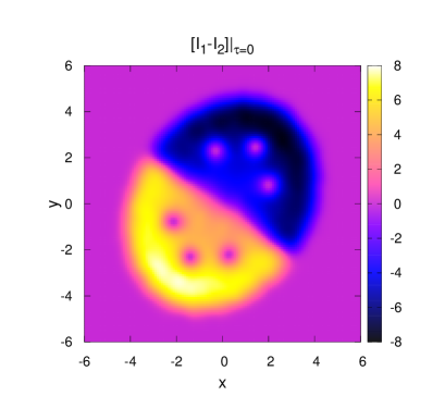
(b)

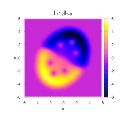
(c)

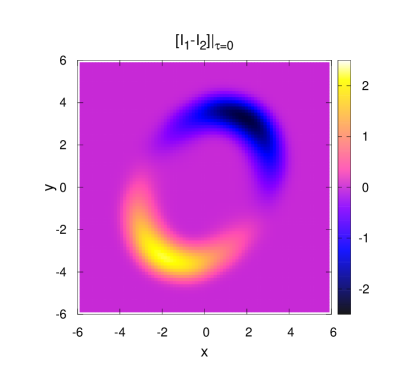
Figure 1: Quasi-two-dimensional configurations for $\zeta=500$, which correspond to rotational frequency $\Omega=0.8$. The difference in the local intensities in cross section $\tau=0$ is demonstrated for three values of chemical potential: (a) $\mu=4$; (b) $\mu=2$, and (c) $\mu=-1$.

(a)

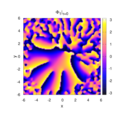
(b)

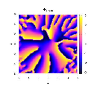
(c)

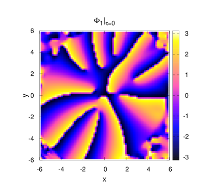
Figure 2: Phase $\Phi_{1}$ of complex envelope $A_{1}$ for the three configurations shown in Fig.1. Panels (a), (b), and (c) correspond to those in Fig.1.

III Results

We have performed two series of numerical experiments. In the first series, we investigated quasi-2D configurations for which the dependence on variable $\tau$ was weak so that vortex filaments were more or less parallel to a domain wall. In the second series of experiments, vortices were oriented as before along the beam, but for $\zeta=0$, two domain walls (on one period in $\tau$) cut across the beam, thus forming regions with right- and left-hand polarizations alternating along the beam axis so that the ends of vortices were attached to the domain walls and strongly deformed them.

The characteristic examples from the first series are shown in Figs. 1 and 2. Since the dynamics remained quasi-2D on the entire interval of $\zeta$, it was sufficient to demonstrate a typical distribution of fields in one of cross sections. Since both intensities $I_{1}$ and $I_{2}$ simultaneously differ from nearly zero only over the domain wall thickness, their difference turns out to be a quite informative quantity. Practically, if it is positive, we are dealing with the left-polarized region, while when it is negative, we have the right-polarized region. It can be seen in Fig.1 that the intensities are maximal not at the waveguide center, but on its periphery. This property is a direct consequence of the action of the “centrifugal force” in the rotating coordinate system. The centrifugal force presses “light liquids” to the waveguide walls. In this respect, Fig.1c corresponding to the negative value of the chemical potential is especially interesting. It can be seen that a wide region exists at the middle of the waveguide, where both intensities are almost equal to zero. This is exactly a nonlinear variant of the whispering gallery effect. Figure 2 showing the phase distribution for the first component corresponding to Fig.1 provides interesting information on the position of vortices. It can be seen that only a part of vortices is located in the region with noticeable intensity $I_{1}$ (patent vortices). These patent vortices avoid the intensity maxima and, hence, are grouped closer to the center. The other part (latent vortices) is located in the region where $I_{1}$ is negligibly small. In Fig.1c, there are no patent vortices, but there is a dozen of latent vortices exactly in the “empty” central region of the waveguide, as follows from Fig.2c.

(a)

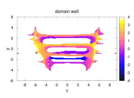
(b)

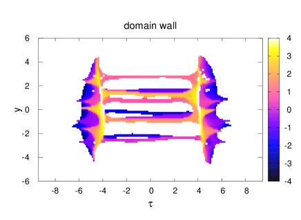
Figure 3: Numerical examples of long-lived transverse domain walls with attached vortices for $\zeta=500$, $\Omega=0.8$ for (a) $\mu=4$ and (b) $\mu=8$. The $x$ coordinate of the points of the numerical grid, at which $0<(I_{1}-I_{2})<d$, where $d=1.0$ in (a) and $d=1.8$ in (b), is marked by the color. This makes it possible to visualize the vortex cores in the first component as well as a thin layer near the middle surface in each domain wall.

As regards the second series of experiments, the essentially 3D evolution of transverse domain walls with attached vortices proceeds differently for different values of $\mu$. For small values of $\mu=0$ and $\mu=1$, such configurations are rapidly “smeared,” and then, after a certain transition process, quasi-2D states similar to those described above are formed. For larger values of $\mu=4$ and $\mu=8$, although the transverse walls acquired on the average a tilted orientation depending on $\zeta$, they continued their existence in the entire interval of $\zeta$ up to the end of calculations. Such a change in the modes of behavior is still unclear. Two examples of 3D structures are shown in Fig.3 (cf. [37]).

It should be noted that for a lower frequency of rotation, the number of vortices decreases, and the tendency to the transverse orientation of domain walls becomes stronger. This tendency conflicts with the aforementioned quasi-2D nature of the flows for small values of $\mu$. As a consequence, a nontrivial intermediate regime becomes possible in a certain range of parameters $(\Omega,\mu)$, when one or two vortices and a nonstationary 3D-perturbed domain wall are present; in this regime, the vortices can sometimes “hide themselves” in this wall partly or completely. Such a dynamics was observed, for example, for $\Omega=0.4$ and $\mu=2$. This regime should be investigated in detail.

IV Conclusions

Thus, we have traced the theoretical analogy between a coherent optical wave in a wide helical waveguide and a rotating binary Bose–Einstein condensate of cold atoms. Some differences between these two systems are observed in the form of the transverse confining potential. For atoms, a quadratic potential can be obtained more easily, while for an optical waveguide, a plane refractive index profile with sharp edges is easier for implementation. Accordingly, the effect of the centrifugal force is stronger in the latter case. This difference leads to different quasi-stationary patterns as can be seen from comparison of the figures in this article with those in [34–37].

This trend in investigations undoubtedly has wide prospects. Although only the first steps have been taken in this direction, nontrivial results have already been obtained and the next goals have been indicated. First of all, parametric region $(N_{1},N_{2},\Omega)$ should be investigated more systematically. In addition, it is important from the practical point of view to study transient dynamic processes because it is difficult to form quasi-stationary states immediately at the waveguide input. Apart from helical waveguides, interesting effects must also exist for some other dependences of the shape of the cross section on coordinate $\zeta$. For example, periodic oscillations of the cross-sectional area or its other geometrical parameters can be responsible for parametric resonances that usually lead in nonlinear systems to the formation of certain coherent structures (see, for example, [32, 33]).

The adequacy of the simplest model (6) in planning and implementation of optical experiment requires further serious investigation. In actual substances, the factors disregarded in this study (e.g., third-order dispersion) can play a certain role. It would be interesting in principle to exceed the limits of the quasi-monochromatic regime and see how the wave pattern will change thereby.

Funding

This study was performed under State assignment no. 0029-2021-0003.

Conflict of interests

The author declares that he has no conflict of interests.

Translated by N. Wadhwa

References

- (1) Y. Kivshar and G. P. Agrawal, Optical Solitons: From Fibers to Photonic Crystals, 1st ed. (Academic, CA, 2003).
- (2) V. E. Zakharov and S. Wabnitz, Optical Solitons: Theoretical Challenges and Industrial Perspectives (Springer, Berlin, 1999).
- (3) B. A. Malomed, Multidimensional Solitons (AIP, Melville, 2022). https://doi.org/10.1063/9780735425118
- (4) F. Baronio, S. Wabnitz, and Yu. Kodama, Phys. Rev. Lett. 116, 173901 (2016).
- (5) P. G. Kevrekidis, D. J. Frantzeskakis, and R. Carretero-González, The Defocusing Nonlinear Schrödinger Equation: From Dark Solitons to Vortices and Vortex Rings (SIAM, Philadelphia, 2015).
- (6) A. L. Berkhoer and V. E. Zakharov, Sov. Phys. JETP 31, 486 (1970).
- (7) Tin-Lun Ho and V. B. Shenoy, Phys. Rev. Lett. 77, 3276 (1996).
- (8) H. Pu and N. P. Bigelow, Phys. Rev. Lett. 80, 1130 (1998).
- (9) B. P. Anderson, P. C. Haljan, C. E. Wieman, and E. A. Cornell, Phys. Rev. Lett. 85, 2857 (2000).
- (10) S. Coen and M. Haelterman, Phys. Rev. Lett. 87, 140401 (2001).
- (11) G. Modugno, M. Modugno, F. Riboli, G. Roati, and M. Inguscio, Phys. Rev. Lett. 89, 190404 (2002).
- (12) E. Timmermans, Phys. Rev. Lett. 81, 5718 (1998).
- (13) P. Ao and S. T. Chui, Phys. Rev. A 58, 4836 (1998).
- (14) M. Haelterman and A. P. Sheppard, Phys. Rev. E 49, 3389 (1994).
- (15) M. Haelterman and A. P. Sheppard, Phys. Rev. E 49, 4512 (1994).
- (16) A. P. Sheppard and M. Haelterman, Opt. Lett. 19, 859 (1994).
- (17) Yu. S. Kivhsar and B. Luther-Davies, Phys. Rep. 298, 81 (1998).
- (18) N. Dror, B. A. Malomed, and J. Zeng, Phys. Rev. E 84, 046602 (2011).
- (19) A. H. Carlsson, J. N. Malmberg, D. Anderson, M. Lisak, E. A. Ostrovskaya, T. J. Alexander, and Yu. S. Kivshar, Opt. Lett. 25, 660 (2000).
- (20) A. S. Desyatnikov, L. Torner, and Yu. S. Kivshar, Progress in Optics 47, 291 (2005).
- (21) V. P. Ruban, JETP Lett. 117, 292 (2023).
- (22) V. P. Ruban, JETP Lett. 117, 583 (2023).
- (23) B. Van Schaeybroeck, Phys. Rev. A 78, 023624 (2008).
- (24) K. Sasaki, N. Suzuki, and H. Saito, Phys. Rev. A 83, 033602 (2011).
- (25) H. Takeuchi, N. Suzuki, K. Kasamatsu, H. Saito, and M. Tsubota, Phys. Rev. B 81, 094517 (2010).
- (26) N. Suzuki, H. Takeuchi, K. Kasamatsu, M. Tsubota, and H. Saito, Phys. Rev. A 82, 063604 (2010).
- (27) H. Kokubo, K. Kasamatsu, and H. Takeuchi, Phys. Rev. A 104, 023312 (2021).
- (28) K. Sasaki, N. Suzuki, D. Akamatsu, and H. Saito, Phys. Rev. A 80, 063611 (2009).
- (29) S. Gautam and D. Angom, Phys. Rev. A 81, 053616 (2010).
- (30) T. Kadokura, T. Aioi, K. Sasaki, T. Kishimoto, and H. Saito, Phys. Rev. A 85, 013602 (2012).
- (31) K. Sasaki, N. Suzuki, and H. Saito, Phys. Rev. A 83, 053606 (2011).
- (32) D. Kobyakov, V. Bychkov, E. Lundh, A. Bezett, and M. Marklund, Phys. Rev. A 86, 023614 (2012).
- (33) D. K. Maity, K. Mukherjee, S. I. Mistakidis, S. Das, P. G. Kevrekidis, S. Majumder, and P. Schmelcher, Phys. Rev. A 102, 033320 (2020).
- (34) K. Kasamatsu, M. Tsubota, and M. Ueda, Phys. Rev. Lett. 91, 150406 (2003).
- (35) K. Kasamatsu and M. Tsubota, Phys. Rev. A 79, 023606 (2009).
- (36) P. Mason and A. Aftalion, Phys. Rev. A 84, 033611 (2011).
- (37) K. Kasamatsu, H. Takeuchi, M. Tsubota, and M. Nitta, Phys. Rev. A 88, 013620 (2013).
- (38) V. P. Ruban, JETP Lett. 113, 814 (2021).
- (39) V. P. Ruban, J. Exp. Theor. Phys. 133, 779 (2021).
- (40) K. J. H. Law, P. G. Kevrekidis, and L. S. Tuckerman, Phys. Rev. Lett. 105, 160405 (2010); Erratum, Phys. Rev. Lett. 106, 199903 (2011).
- (41) M. Pola, J. Stockhofe, P. Schmelcher, and P. G. Kevrekidis, Phys. Rev. A 86, 053601 (2012).
- (42) S. Hayashi, M. Tsubota, and H. Takeuchi, Phys. Rev. A 87, 063628 (2013).
- (43) G. C. Katsimiga, P. G. Kevrekidis, B. Prinari, G. Biondini, and P. Schmelcher, Phys. Rev. A 97, 043623 (2018).
- (44) A. Richaud, V. Penna, R. Mayol, and M. Guilleumas, Phys. Rev. A 101, 013630 (2020).
- (45) A. Richaud, V. Penna, and A. L. Fetter, Phys. Rev. A 103, 023311 (2021).
- (46) V. P. Ruban, JETP Lett. 113, 532 (2021).
- (47) V. P. Ruban, JETP Lett. 115, 415 (2022).
- (48) V. P. Ruban, W. Wang, C. Ticknor, and P. G. Kevrekidis, Phys. Rev. A 105, 013319 (2022).
- (49) X. Liu, B. Zhou, H. Guo, and M. Bache, Opt. Lett. 40, 3798 (2015).
- (50) X. Liu and M. Bache, Opt. Lett. 40, 4257 (2015).