Time-dependent probability density function for partial resetting dynamics

Abstract

Stochastic resetting is a rapidly developing topic in the field of stochastic processes and their applications. It denotes the occasional reset of a diffusing particle to its starting point and effects, inter alia, optimal first-passage times to a target. Recently the concept of partial resetting, in which the particle is reset to a given fraction of the current value of the process, has been established and the associated search behaviour analysed. Here we go one step further and we develop a general technique to determine the time-dependent probability density function (PDF) for Markov processes with partial resetting. We obtain an exact representation of the PDF in the case of general symmetric Lévy flights with stable index $0<\alpha\leq 2$. For Cauchy and Brownian motions (i.e., $\alpha=1,2$), this PDF can be expressed in terms of elementary functions in position space. We also determine the stationary PDF. Our numerical analysis of the PDF demonstrates intricate crossover behaviours as function of time.

1 Introduction

Stochastic processes represent a core field in non-equilibrium statistical physics and physical chemistry [1, 2]. They are used as "schematisations" [3] for systems, that are too complex to describe in microscopic detail [4], and in which the dynamic of an observable is apparently random. Stochastic processes are quite ubiquitous in nature. Examples include, inter alia, archetypical Brownian motion [5], the passive diffusion of molecules in biological cells [6], animal motion [7], the motion of active particles beyond their persistence time [8], tracer motion in geophysical systems [9], charge carrier motion in semiconductors [10], stock prices on financial markets [11], or disease spreading [12].

One central question in the study of stochastic processes is their ability to locate a specific target in space [13]. In an unlimited space a diffusing particle may significantly stray away from its starting point and may not be able to locate a small target in a finite interval of time. Even in a finite domain the diffusive search may have very broad distributions of search times, and the typical search time may be significantly different from the mean [14, 15, 16]. Speedup of the diffusive search may, e.g., be achieved by "facilitated diffusion", in which the diffusion intermittently occurs in the embedding space and on a surface with reduced dimension—a prominent example is the search of binding proteins for a site on a long DNA chain [17, 18]. The central idea in facilitated diffusion is the combination of thorough local search and decorrelations by bulk diffusion [19, 20]. Similar principles in random search are processes with long-tailed jump length distributions (Lévy flights and walks) [21, 22, 23, 24, 25, 26, 27, 28, 29, 30] and intermittent search [13, 31, 32, 33].

Another way to optimise the search for a target at a finite distance away from where the searching particle is released, is stochastic resetting (SR) [34, 35]. In its simplest version, SR considers a Brownian particle, that experiences repeated restarts, i.e., resets to its starting position, either at fixed periods or stochastically with a fixed rate [34, 35, 36, 37, 38]. A central feature of SR is that the stochastic search of a diffusing particle for a target at a given distance from its starting point can be optimised for a specific resetting frequency [34, 35, 36]. The idea is that SR prevents long departures of the particle away from its target. Overly frequent resetting, in contrast, keeps the particle always close to the starting point, such that it cannot reach the target. At intermediate resetting frequencies, therefore, the mean search time is minimised [34, 35, 36]. For mean search times a unified approach allows to determine the optimal SR-rate [39] and, at optimality, first-passage time fluctuations have a universal coefficient of variation [40], see also recent results on extremes in SR [41]. SR leads to a non-equilibrium steady state with a well-defined limiting displacement distribution [34, 35, 36]. A renewal approach to resetting was established and exploited to show that constant pace resetting minimises the mean hitting time [42]. Moreover, linear response and fluctuation-dissipation relations for SR were discussed [43]. Aspects of SR in quantum walks have also been addressed [44]. A recent review of SR and applications in different disciplines can be found in [45]. Importantly, we mention that the effect of SR was demonstrated experimentally [46, 47, 48].

Various aspects beyond Brownian SR have been discussed. Inter alia, non-instantaneous returns [49] and soft resetting by switching harmonic potentials [50] were studied. SR of anomalous diffusion processes include heterogeneous diffusion processes with distance-dependent diffusion coefficient [51, 52], scaled Brownian motion with time-dependent diffusivity in renewal and non-renewal settings [53, 54], and continuous time random walk processes with complete and incomplete [55] as well as with power-law [56] resetting. Reset rotational motion was studied in terms of a time-fractional Fokker-Planck equation [57]. Different effects due to resetting were demonstrated for geometric Brownian motion without [58] and with drift [59], and effects on income dynamics explored [60]. Aspects of ergodicity restoration in anomalous diffusion processes were also analysed [61]. For SR on networks [62, 63, 64], the minimisation of global mean first passage times for specific centrality-based SR mechanisms were reported [65]. We note that results similar to SR for a single absorbing target were obtained for multiple as well as partially absorbing targets [66, 67]. Moreover, a concept similar to SR is preferential relocations, which take the walker back to any previously visited site [69, 68].

Here we address the question as to what happens when the particle is not reset to its origin, but to some value in between the instantaneous co-ordinate and the initial value. Such partial stochastic resetting (PSR) has been studied in mathematical [70, 71], financial and actuarial [72, 73, 75, 76, 74] literature, and in queueing theory [77] for piecewise deterministic processes. The basic idea behind many models in these fields is that there is a growing observable (like the income of an insurance company or the amount of traffic over the internet), subjected to random unexpected events leading to a substantial decrease of this quantity (claims in an insurance company or failures in internet connections). PSR has also been recently considered in physics literature [78], where the authors studied the two distinct cases of independent and dependent random resetting amplitudes: for independent resetting, the amplitude is arbitrary, so that the particle can also be reset to negative values, while for dependent resetting amplitudes the current value of the particle is multiplied by a number between zero and unity, thus guaranteeing positivity of the value after reset. In [78] the authors discussed PSR for both scenarios in terms of moments and the particle probability density function (PDF). The case of dependent resetting was recently also analysed further [79, 80]. PSR finds its motivation in different settings. One is stratigraphy, studying sediment layering in geology [78]: deposits by a gradual sedimentation, e.g., in a river delta, can be partially washed away by sudden events such as extreme rainfall. A similar model is used in population dynamics, when the gradual growth dynamic is interrupted by sudden, catastrophic population decimation [82, 83, 84, 81, 85].

Going significantly beyond recent work [79, 80] reporting the Fokker-Planck equation and the stationary PDF for Brownian PSR [79] and the time-dependent PDF in Fourier-Laplace space when the initial condition is at the origin, we here develop a general technique to determine the time-dependent PDF for homogeneous Markov processes with Poissonian resetting, in which the process is partially reset by multiplication with the constant factor $0<c<1$ at random times $T_{1},T_{1}+T_{2},\ldots$. The limiting cases $c\to 0$ and $c\to 1$ of this model correspond to total resetting [34] and a stochastic process without resetting, respectively. An exact representation of the PDF in the real space-time domain is derived for the case of general symmetric Lévy flights with stable index $0<\alpha\leq 2$, including Brownian motion and Cauchy flights as particular cases for $\alpha=2$ and $1$, respectively. We also determine the stationary PDF for symmetric Lévy flights in terms of Fox $H$-functions and present the particular cases $\alpha=2$ and $1$ in terms of elementary functions. For the case of non-zero initial conditions, we report highly asymmetric non-stationary PDFs for $\alpha=2$ and the emergence of non-trivial inhomogeneous multimodal regimes with $\alpha\neq 2$.

2 Propagator for partial resetting

We consider a stochastic process $X_{t}$ with initial condition $X_{0}=x_{0}$ whose PDF is $p_{0}(x,t|x_{0},t_{0})$. We assume homogeneity in both space and time, such that $p_{0}(x,t|x_{0},t_{0})=p_{0}(x-x_{0},t-t_{0}|0,0)$. Without limitation of generality, we set $t_{0}=0$ and use the simplified notation $p_{0}(x,t)$, keeping the initial condition $x_{0}$ implicit. At random times $T_{1},T_{1}+T_{2},T_{1}+T_{2}+T_{3},\ldots$, the position of the particle is partially reset, i.e., multiplied by $0<c<1$. Thus $T_{i}$ represents the time between the $(i-1)$st and $i$th partial reset. We assume that the $T_{i}$ are independent, identically distributed (i.i.d.) random variables with PDF $\psi(t)=\mathrm{Pr}\{t\leq T_{1}\leq t+dt\}$. Clearly, $c=0$ represents the full resetting case, while setting $c=1$ we retrieve the unperturbed stochastic process. Let $Y_{t}$ denote the PSR process. We then have

$$Y_{t} = x_{0}+\left[\left(\left(X_{T_{1}}\cdot c+X_{T_{2}}\right)\cdot c+X_{T_{3}}\right)\cdot c+\dots\right]\cdot c+X_{t-T_{N_{t}}}$$ (1)

$$= x_{0}+c^{N_{t}}X_{T_{1}}+c^{N_{t}-1}X_{T_{2}}+\dots cX_{T_{N_{t}}}+X_{t-T_{N_{t}}},$$

where $N_{t}$ denotes the number of partial resetting events in the time interval $[0,t]$. The meaning of this expression is quite intuitive: the process is unperturbed until the time $T_{1}$, moving from $x_{0}$ to $x_{0}+X_{T_{1}}$; then the process is multiplied by $c$, and it stays unperturbed again between times $T_{1}$ and $T_{1}+T_{2}$, and so on. Some possible trajectories of $Y_{t}$ are depicted in figure for Brownian and Cauchy random walks (see below) in absence and presence of PSR 1. Generally we notice that in the presence of PSR the resulting trajectories tend to be closer to the origin, while they experience long excursions in the unperturbed case. This hints at the existence of a stationary state, that we will examine more closely below.

Figure 1: Plot of two possible trajectories of the system in the specific cases of Brownian motion (left panel) and symmetric Cauchy random walk (right panel). The process without PSR ($X_{t}$) is depicted in blue on both panels, while the process with PSR ($Y_{t}$, with rate $r=1.0$ and amplitude factor $c=0.5$) is displayed in green. We highlighted partial resetting events with red segments. The processes $X_{t}$ and $Y_{t}$ in either panel were generated from the same random seed.

We are interested in finding the PDF $p_{r}(x,t|x_{0})$ of the PSR process $Y_{t}$. Since we choose $X_{t}$ to be time-homogeneous, it follows that $Y_{t}$ is also homogeneous in time. However, partial resetting according to equation (1) leads to an inhomogeneity in space. Thus, in the PDF $p_{r}(x,t|x_{0})$ we removed the dependence on the initial time $t_{0}$ (taken as $t_{0}=0$) but we retain the dependence on $x_{0}$. The reason for the loss of spatial homogeneity is quite intuitive: consider the first partial resetting event, occurring at time $T_{1}$. The position $Y_{T_{1}^{+}}$ depends on $Y_{T_{1}^{-}}$, and $Y_{T_{1}^{-}}$ in turn depends on $x_{0}$. Due to partial resetting the shape of the resulting time-dependent PDF due to this effect attains more complicated shapes, as we will discuss in the next sections.

For the specific case of Poissonian resetting times, i.e., $\psi(t)=re^{-rt}$ for all $i$, the expression of $p_{r}$ can be found through the last renewal equation, which reads

$$p_{r}(x,t|x_{0})=e^{-rt}p_{0}(x,t|x_{0})+\int_{0}^{t}dt^{\prime}re^{-rt^{\prime}}\int_{-\infty}^{\infty}dyp_{r}(y,t-t^{\prime}|x_{0})p_{0}(x,t^{\prime}|cy).$$ (2)

The meaning of this relation is quite simple: the first term on the right hand side takes into consideration all realisations in which no partial resetting occurred, while the second term considers all realisations in which the last resetting event occurred at time $t-t^{\prime}$. During the time interval $[0,t-t^{\prime}]$ the particle diffuses to position $y$ with propagator $p_{r}(y,t-t^{\prime}|x_{0})$, while during $[t-t^{\prime},t]$ it diffuses without PSR, hence with $p_{0}(x,t^{\prime}|cy)$. This term must be integrated over all possible realisations of $t^{\prime}$ and $y$. The solution of the integral equation (2) can be obtained via the series expansion

$$p_{r}(x,t|x_{0})=e^{-rt}\sum_{n=0}^{\infty}r^{n}q_{n}(x,t|x_{0}),$$ (3)

where the set of functions $\{q_{n}\}_{n=0}^{\infty}$ can be found through the recursion relation

$$q_{0}(x,t|x_{0})=p_{0}(x,t|x_{0}),\quad q_{n}(x,t|x_{0})=\int_{0}^{t}dt^{\prime}\int_{-\infty}^{\infty}dyq_{n-1}(y,t^{\prime}|x_{0})p_{0}(x,t-t^{\prime}|cy).$$ (4)

We proof this result in A. In the recursion relation (4) we now perform a Laplace transform to obtain

$$\tilde{q}_{n}(x,s|x_{0})=\int_{-\infty}^{\infty}dy\tilde{q}_{n-1}(y,s|x_{0})\tilde{p}_{0}(x-cy,s).$$ (5)

Note that the explicit dependence on $x_{0}$ is also inherent in these transformed functions. Applying an additional Fourier transform,

$$\hat{\tilde{q}}_{n}(k,s|x_{0})=\hat{\tilde{q}}_{n-1}(kc,s|x_{0})\hat{\tilde{p}}_{0}(k,s).$$ (6)

Thus we can find the general expression by simply iterating

$$\hat{\tilde{q}}_{n}(k,s|x_{0})=\left(\prod_{l=0}^{n-1}\hat{\tilde{p}}_{0}(kc^{l},s)\right)\hat{\tilde{p}}_{0}(kc^{n},s|x_{0}).$$ (7)

Since $p_{0}$ is spatial homogeneous we can use the relation $\hat{\tilde{p}}_{0}(kc^{n},s|x_{0})=e^{ikc^{n}x_{0}}\hat{\tilde{p}}_{0}(kc^{n},s)$ to obtain

$$\hat{\tilde{q}}_{n}(k,s|x_{0})=e^{ikc^{n}x_{0}}\prod_{l=0}^{n}\hat{\tilde{p}}_{0}(kc^{l},s).$$ (8)

Hence, combining (3) and (8) we may write the full PDF in Fourier-Laplace space as

$$\hat{\tilde{p}}_{r}(k,s|x_{0})=\sum_{n=0}^{\infty}r^{n}e^{ikc^{n}x_{0}}\prod_{l=0}^{n}\hat{\tilde{p}}_{0}(kc^{l},r+s).$$ (9)

Equation (9) is the first main result of the paper, generalising previous results [78, 80, 79]. In [78] the authors considered the case of deterministic ballistic motion with constant speed and PSR. The propagator for this process which was not reported in [78] can be found from result (9) by setting $p_{0}(x,t)=\delta(x-vt)$, where $v$ is the speed. Moreover, the results in [80, 79] follow from (9) by setting $x_{0}=0$ and $p_{0}(x,t)=(4\pi Dt)^{-1/2}\exp(-x^{2}/(4Dt))$.

For consistency, we check the limit of $c\to 1$, for which we find

$$\hat{\tilde{p}}_{r}(k,s|x_{0}) = e^{ikx_{0}}\hat{\tilde{p}}_{0}(k,r+s)\sum_{n=0}^{\infty}\left(r\hat{\tilde{p}}_{0}(k,r+s)\right)^{n}=e^{ikx_{0}}\hat{\tilde{p}}_{0}(k,r+s)\dfrac{1}{1-r\hat{\tilde{p}}_{0}(k,r+s)}$$ (10)

$$= e^{ikx_{0}}\hat{\tilde{p}}_{0}(k,s),$$

where in the last step we used an identity for Markov processes proved in B. As expected, we retrieve the PDF for the stochastic process without resetting. In the case $c\to 0$, we obtain

$$\hat{\tilde{p}}_{r}(k,s|x_{0})=\hat{\tilde{p}}_{0}(k,r+s)\sum_{n=0}^{\infty}\left(\dfrac{r}{r+s}\right)^{n}=\dfrac{r+s}{s}\hat{\tilde{p}}_{0}(k,r+s),$$ (11)

which is the same result as the one for total resetting [45].

3 Lévy flights

Let us consider now the general case in which the underlying process $X_{t}$ is a symmetric Lévy flight [11, 88]. The associated characteristic function $\hat{p}_{0}(k,t)$ of a symmetric Lévy stable PDF is then given by [88, 90, 89, 91, 92]

$$\hat{p}_{0}(k,t)=e^{-D|k|^{\alpha}t},$$ (12)

which in Fourier-Laplace space reads (see also [93])

$$\hat{\tilde{p}}_{0}(k,s)=\dfrac{1}{s+D|k|^{\alpha}}.$$ (13)

In real space this PDF becomes

$$p_{0}(x,t)=\int_{0}^{\infty}\dfrac{dk}{\pi}\cos\left(kx\right)e^{-D|k|^{\alpha}t},$$ (14)

with $\alpha\in(0,2]$. The case $\alpha=2$ corresponds to a Gaussian PDF, while for $\alpha\in(0,2)$ the asymptotic scaling of the PDF has the power-law tails $p_{0}(x,t)\simeq|x|^{-1-\alpha}$ [88, 91, 92, 90, 89]. The inverse Fourier transform in (14) can be performed by use of Fox $H$-functions (see below), while in the special cases $\alpha=1,2$ simple, explicit forms for the PDF $p_{0}(x,t)$ can be found in terms of a Cauchy PDF and a normal Gaussian, respectively. We will treat these two special cases in detail in the next sections.

In Fourier-Laplace space, using equations (8) and (13) we obtain the functions

$$\hat{\tilde{q}}_{n}(k,s|x_{0})=e^{ikc^{n}x_{0}}\prod_{l=0}^{n}\dfrac{1}{s+Dc^{\alpha l}|k|^{\alpha}},$$ (15)

and with equation (9) we find

$$\hat{\tilde{p}}_{r}(k,s|x_{0})=\sum_{n=0}^{\infty}r^{n}e^{ikc^{n}x_{0}}\prod_{l=0}^{n}\dfrac{1}{r+s+Dc^{\alpha l}|k|^{\alpha}}.$$ (16)

This PDF solves the fractional Fokker-Planck equation (as shown in C)

$$\frac{\partial p_{r}(x,t|x_{0})}{\partial t}=D\frac{\partial^{\alpha}}{\partial|x|^{\alpha}}p_{r}(x,t|x_{0})-rp_{r}(x,t|x_{0})+\frac{r}{c}p_{r}\left(\frac{x}{c},t|x_{0}\right),$$ (17)

where the space-fractional operator is defined in terms of its Fourier transform, $\mathscr{F}\{\partial^{\alpha}g(x)/\partial|x|^{\alpha}\}=-|k|^{\alpha}g(k)$ [94]. Setting $\alpha=2$ and $x_{0}=0$ we retrieve the dynamic equation obtained in [80] corresponding to Brownian motion with PSR, see also below. For $0<c<1$ we can simplify equation (15) by using the partial fraction decomposition

$$\hat{\tilde{q}}_{n}(k,s|x_{0})=\dfrac{e^{ikc^{n}x_{0}}}{s^{n}}\sum_{m=0}^{n}\dfrac{1}{(c^{-\alpha};c^{-\alpha})_{m}(c^{\alpha};c^{\alpha})_{n-m}}\dfrac{1}{s+Dc^{\alpha m}|k|^{\alpha}},$$ (18)

where the symbols in the parentheses denote the $q$-Pochhammer symbol defined as [95]

$$(a;q)_{n}=\prod_{l=0}^{n-1}(1-aq^{l}).$$ (19)

After inverse Laplace transform of $\hat{\tilde{q}}_{n}$ we obtain

$$\hat{q}_{0}(k,t|x_{0})=e^{ikc^{n}x_{0}-D|k|^{\alpha}t},$$ (20)

for $n=0$ and, by use of the convolution theorem,

$$\hat{q}_{n}(k,t|x_{0})=e^{ikc^{n}x_{0}}\sum_{m=0}^{n}\dfrac{1}{(c^{-\alpha};c^{-\alpha})_{m}(c^{\alpha};c^{\alpha})_{n-m}}\int_{0}^{t}dt^{\prime}\dfrac{(t-t^{\prime})^{n-1}}{(n-1)!}e^{-Dc^{\alpha m}|k|^{\alpha}t^{\prime}}$$ (21)

for $n\geq 1$. We now perform an inverse Fourier transform,

$$q_{n}(x,t|x_{0})=\sum_{m=0}^{n}\dfrac{1}{(c^{-\alpha};c^{-\alpha})_{m}(c^{\alpha};c^{\alpha})_{n-m}}\int_{0}^{t}dt^{\prime}\dfrac{(t-t^{\prime})^{n-1}}{(n-1)!}p_{0}(x-c^{n}x_{0},c^{\alpha m}t^{\prime}),$$ (22)

for $n\geq 1$. Then the formula for the propagator may be written in the compact form

$$p_{r}(x,t|x_{0}) = e^{-rt}\sum_{n=0}^{\infty}r^{n}\sum_{m=0}^{n}\dfrac{1}{(c^{-\alpha};c^{-\alpha})_{m}(c^{\alpha};c^{\alpha})_{n-m}}$$ (23)

$$\times\int_{0}^{t}dt^{\prime}\left((1-\delta_{n0})\dfrac{(t-t^{\prime})^{n-1}}{(n-1)!}+\delta_{n0}\delta(t-t^{\prime})\right)p_{0}(x-c^{n}x_{0},c^{\alpha m}t^{\prime}),$$

where $\delta_{ij}$ denotes the Kronecker delta and $\delta(t)$ denotes the Dirac $\delta$-function. The formula above is the second main result of the paper.

Let us show that expression (23) is indeed normalised. To this end we integrate over $x$. Since $p_{0}$ is normalised, we get

$$\int_{-\infty}^{\infty}dxp_{r}(x,t|x_{0})=e^{-rt}\sum_{n=0}^{\infty}\dfrac{(rt)^{n}}{n!}\sum_{m=0}^{n}\dfrac{1}{(c^{-\alpha};c^{-\alpha})_{m}(c^{\alpha};c^{\alpha})_{n-m}}.$$ (24)

We prove in D that

$$\sum_{m=0}^{n}\dfrac{1}{(c^{-\alpha};c^{-\alpha})_{m}(c^{\alpha};c^{\alpha})_{n-m}}=1,$$ (25)

and therefore $p_{r}(x,t|x_{0})$ in (23) is normalised, as it should be.

3.1 Stationary distribution

The stationary distribution for Lévy flight-PSR can be obtained by setting the time derivative in (17) to $0$ and applying an inverse Fourier transform,

$$-D|k|^{\alpha}\hat{p}^{(s)}_{r}(k)-r\hat{p}^{(s)}_{r}(k)+r\hat{p}^{(s)}_{r}(kc)=0,$$ (26)

which after iteration produces

$$\hat{p}^{(s)}_{r}(k)=\prod_{l=0}^{\infty}\dfrac{r}{r+Dc^{\alpha l}|k|^{\alpha}}.$$ (27)

In the limiting case $\alpha=2$ we obtain the same result as in [80, 79]. We may ask whether by taking the limit $t\to\infty$ in the general expression (16) for the propagator we get the same formula (27). This agreement can indeed be demonstrated, compare the use of Cesaro’s and final value theorems for the specific case $\alpha=2$ as shown in one of the appendices of [80]. The derivation can be directly extended for the generic $\alpha$. Equation (27) can be transformed by using partial fraction decomposition, yielding

$$\hat{p}^{(s)}_{r}(k)=\sum_{n=0}^{\infty}\dfrac{r}{r+Dc^{\alpha n}|k|^{\alpha}}\prod_{\begin{subarray}{c}l=0,l\neq n\end{subarray}}^{\infty}\dfrac{1}{1-c^{\alpha(l-n)}}=\dfrac{1}{(c^{\alpha};c^{\alpha})_{\infty}}\sum_{n=0}^{\infty}\dfrac{1}{(c^{-\alpha};c^{-\alpha})_{n}}\dfrac{r}{r+Dc^{\alpha n}|k|^{\alpha}},$$ (28)

which is the third main result of the paper. We note that for $k=0$, by using a well-known identity for $q$-Pochhammer symbols first discovered by Euler [95],

$$\dfrac{1}{(c^{\alpha};c^{\alpha})_{\infty}}\sum_{n=0}^{\infty}\dfrac{1}{(c^{-\alpha};c^{-\alpha})_{n}}=1,$$ (29)

we see that the PDF is normalised. After inverse Fourier transform in equation (28) we obtain the stationary PDF in position space,

$$p^{(s)}_{r}(x)=\dfrac{1}{(c^{\alpha};c^{\alpha})_{\infty}}\sum_{n=0}^{\infty}\dfrac{1}{(c^{-\alpha};c^{-\alpha})_{n}}\int_{0}^{\infty}\dfrac{dk}{\pi}\cos(kx)\dfrac{r}{r+Dc^{\alpha n}|k|^{\alpha}}.$$ (30)

This is another central result of this paper.

In the last expression the Fourier cosine integral can be solved analytically in terms of Fox $H$-functions [98]. To this end we note first that the image function can be identified with the $H$-function

$$\frac{1}{1+\frac{D}{r}c^{\alpha n}|k|^{\alpha}}=H^{1,1}_{1,1}\left[\frac{D}{r}c^{\alpha n}|k|^{\alpha}\left|\begin{array}[]{ll}(0,1)\\ (0,1)\end{array}\right.\right]=\frac{1}{\alpha}H^{1,1}_{1,1}\left[\left(\frac{D}{r}\right)^{1/\alpha}c^{n}|k|\left|\begin{array}[]{ll}(0,1/\alpha)\\ (0,1/\alpha)\end{array}\right.\right],$$ (31)

where in the second step we made use of a well known theorem of $H$-functions [98]. The cosine transform then is merely a manipulation of indices [99], and we find

$$p^{(s)}_{r}(x)=\dfrac{1}{(c^{\alpha};c^{\alpha})_{\infty}}\sum_{n=0}^{\infty}\dfrac{1}{(c^{-\alpha};c^{-\alpha})_{n}}\frac{1}{\alpha|x|}H^{2,1}_{2,3}\left[\frac{\lambda^{1/\alpha}|x|}{c^{n}}\left|\begin{array}[]{ll}(1,1/\alpha),(1,1/2)\\ (1,1),(1,1/\alpha),(1,1/2)\end{array}\right.\right],$$ (32)

another main result of this work. Here we defined $\lambda=r/D$. We will consider in detail the cases $\alpha=1,2$ in the following sections.

4 Brownian motion with PSR

In the Gaussian case $\alpha=2$ the PDF $p_{0}$ reads

$$p_{0}(x,t)=\dfrac{1}{\sqrt{4\pi Dt}}\exp\left(-\dfrac{x^{2}}{4Dt}\right),$$ (33)

hence the propagator (23) becomes

$$p_{r}(x,t|x_{0}) = e^{-rt}\frac{1}{\sqrt{4\pi Dt}}\exp\left(-\dfrac{(x-x_{0})^{2}}{4Dt}\right)+re^{-rt}\sum_{n=1}^{\infty}\int_{0}^{t}dt^{\prime}\frac{[r(t-t^{\prime})]^{n-1}}{(n-1)!}$$ (34)

$$\times\sum_{m=0}^{n}\mathcal{C}^{(2)}_{n,m}\frac{1}{\sqrt{4\pi Dc^{2m}t^{\prime}}}\exp\left(-\frac{(x-c^{n}x_{0})^{2}}{4Dc^{2m}t^{\prime}}\right).$$

Here we used the abbreviation

$$\mathcal{C}_{n,m}^{(\alpha)}=\frac{1}{\left(c^{-\alpha};c^{-\alpha}\right)_{m}\left(c^{\alpha};c^{\alpha}\right)_{n-m}}.$$ (35)

The integral over time can be performed analytically, yielding

$$p_{r}(x,t|x_{0}) = e^{-rt}\frac{1}{\sqrt{4\pi Dt}}\exp\left(-\frac{(x-x_{0})^{2}}{4Dt}\right)+re^{-rt}\sum_{n=1}^{\infty}\frac{(rt)^{n-1}}{2D(n-1)!\Gamma\left(n+\frac{1}{2}\right)}$$ (36)

$$\times\sum_{m=0}^{n}\mathcal{C}^{(2)}_{n,m}c^{-2m}\biggr{[}(n-1)!c^{m}\sqrt{Dt}\,_{1}F_{1}\left(-n+\frac{1}{2};\frac{1}{2};-\frac{\left(x-c^{n}x_{0}\right)^{2}}{4Dc^{2m}t}\right)+$$

$$-\Gamma\left(n+\frac{1}{2}\right)\left|x-c^{n}x_{0}\right|\,_{1}F_{1}\left(1-n;\frac{3}{2};-\frac{\left(x-c^{n}x_{0}\right)^{2}}{4Dc^{2m}t}\right)\biggr{]},$$

where ${}_{1}F_{1}$ denotes the Kummer confluent hypergeometric function. We note that in [80], the authors derived the Fourier-Laplace transform of the propagator for the special initial condition $x_{0}=0$. Our results above extend this result to an arbitrary initial condition and we invert this general form to real space.

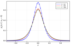
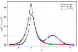
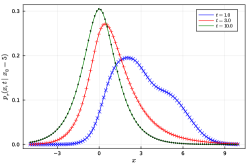
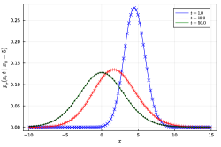
(a) (b) (c) (d) with time.

Figure 2: Propagator for Brownian motion with partial resetting. Solid lines represent the analytical distribution (36), while symbols represent the simulations results. In (a) the starting position is $x_{0}=0$, while in (b)-(d) it is $x_{0}=5$. The resetting factor $c$ was chosen as $c=0.5$ in (a), $c=0.1$ in (b), $c=0.5$ in (c), and $c=0.9$ in (d).

The PDF (36) is shown in figures 2 and 3 for different choices of the parameters. The agreement between theory and simulations is excellent. The simulated PDF was obtained with the algorithm described in E. We note that while the PDF stays symmetric around the origin when the process is initiated in $x=0$, when the initial condition is away from the origin, strong asymmetries of the PDF are observed. These asymmetries relax as function of time, and eventually convergence to a stationary, symmetric form. As seen in figure 2 the relaxation to stationarity requires more time when the resetting factor $c$ is closer to the value $c=1$ in absence of any resetting.

To obtain a concrete form for the stationary distribution, we set $\alpha=2$ in equation (32) to get

$$p^{(s)}_{r}(x)=\frac{1}{2(c^{2};c^{2})_{\infty}}\sqrt{\frac{r}{D}}\sum_{n=0}^{\infty}\frac{c^{-n}}{(c^{-2};c^{-2})_{n}}e^{-\sqrt{r/D}\ c^{-n}|x|},$$ (37)

which is in agreement with [79].

Figure 3: Propagator for Brownian motion with PSR with starting position $x_{0}=5$, and for different values of the resetting factor $c$. The time is chosen as (a) $t=1$ and (b) $t=10$.

5 PSR for the Cauchy case

In the case $\alpha=1$, for which the Lévy stable density is given by the Cauchy (Lorentz) distribution, the function $p_{0}$ reads

$$p_{0}(x,t)=\dfrac{1}{\pi}\dfrac{Dt}{x^{2}+D^{2}t^{2}}.$$ (38)

With equation (23) we therefore find

$$p_{r}(x,t|x_{0})=\dfrac{Dt}{x^{2}+D^{2}t^{2}}+re^{-rt}\sum_{n=1}^{\infty}\int_{0}^{t}dt^{\prime}\dfrac{\left[r(t-t^{\prime})^{n-1}\right]}{\pi(n-1)!}\sum_{m=0}^{n}\mathcal{C}_{n,m}^{(1)}\dfrac{1}{\pi}\dfrac{Dc^{m}t^{\prime}}{(x-c^{n}x_{0})^{2}+(Dc^{m}t^{\prime})^{2}}.$$ (39)

The integral can be performed analytically, yielding

$$p_{r}(x,t|x_{0}) = \dfrac{1}{\pi}\dfrac{Dt}{x^{2}+D^{2}t^{2}}+\dfrac{1}{\pi}e^{-rt}\sum_{n=1}^{\infty}\dfrac{(rt)^{n}}{(n+1)!}\sum_{m=0}^{n}\mathcal{C}_{n,m}^{(1)}\dfrac{Dc^{m}t}{(x-c^{n}x_{0})^{2}}$$ (40)

$$\times\,_{3}F_{2}\left(1,1,\frac{3}{2};\frac{n}{2}+1,\frac{n}{2}+\frac{3}{2};\dfrac{-D^{2}c^{2m}t^{2}}{(x-c^{n}x_{0})^{2}}\right),$$

where ${}_{p}F_{q}(a_{1},\dots,a_{p};b_{1},\dots,b_{p};z)$ is the generalised hypergeometric function [95]. The stationary PDF follows from equation (30). The integral for $\alpha=1$ is computed explicitly in reference [87], and we find

$$p^{(s)}_{r}(x) = \dfrac{1}{\pi(c^{\alpha};c^{\alpha})_{\infty}}\sum_{n=0}^{\infty}\dfrac{1}{(c^{-\alpha};c^{-\alpha})_{n}}\dfrac{\lambda}{c^{n}}$$ (41)

$$\times\left[\left(\dfrac{\pi}{2}-\text{Si}\left(\dfrac{\lambda|x|}{c^{n}}\right)\right)\sin\left(\dfrac{\lambda|x|}{c^{n}}\right)-\cos\left(\dfrac{\lambda x}{c^{n}}\right)\text{Ci}\left(\dfrac{\lambda|x|}{c^{n}}\right)\right],$$

where we again used $\lambda=r/D$, and where the sine/cosine integrals $\text{ Si}(x)$ and $\text{Ci}(x)$ are defined as

$$\text{Si}(x)=\int_{0}^{x}\dfrac{\sin(t)}{t}dt,\quad\text{Ci}(x)=\int_{x}^{\infty}\dfrac{\cos(t)}{t}dt.$$ (42)

In the case of total resetting with $c=0$, this result coincides with the one obtained in [87].

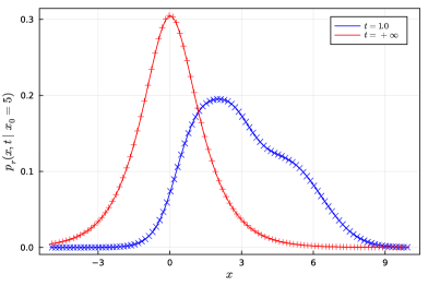
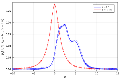
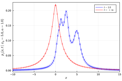
(a) (b) (c) (d)

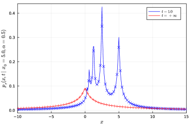
Figure 4: Propagator for Brownian motion and Lévy flight with PSR for (a) $\alpha=2$ (Brown), (b) $\alpha=1.5$, (c) $\alpha=1.0$ (Cauchy), and (d) $\alpha=0.5$. Parameters: $x_{0}=5$, $D=1$, $r=1$, $t=1$, and $c=0.5$.

In figure 4 we plot the PDF (40) and the associated stationary PDF (41) along with examples for Gaussian and other Lévy flight processes with $\alpha=2.0$, $\alpha=1.5$, and $\alpha=0.5$. For the latter cases expression (23) was evaluated numerically. The agreement with numerical simulations is excellent in all cases. A distinct feature are the strong asymmetries in the PDF due to the initial condition. For lower $\alpha$, i.e., longer-tailed stable densities, the multimodal structure becomes more spiky. The multimodality of the PDF can be anticipated from equation (3), according to which the PDF is a sum of single-peaked functions centred on different positions.

6 Conclusions

We established a framework to calculate the time-dependent PDF in the presence of partial resetting effects for homogeneous Markov processes with Poissonian resetting, in which the process is partially reset by multiplication with a constant factor $0<c<1$ at random times. We showed that, consistently, the limiting cases $c\to 0$ and $c\to 1$ of this model correspond to total resetting [34] and a stochastic process without resetting, respectively. We derived an exact representation of the PDF in the real space-time domain for the case of general symmetric Lévy flights with stable index $0<\alpha\leq 2$, including Brownian motion and Cauchy flights as particular cases for $\alpha=2$ and $1$. As our approach is valid for generic Markov processes, in the future other densities such as asymmetric Lévy stable forms can be studied. For the case of non-zero initial conditions, we reported highly asymmetric non-stationary PDFs for $\alpha=2$ and the emergence of non-trivial inhomogeneous multimodal regimes with $\alpha\neq 2$. We also determined the stationary PDF for symmetric Lévy flights in terms of Fox $H$-functions and presented the particular cases $\alpha=2$ and $1$ in terms of elementary functions. Moreover, we also showed how the resetting factor $c$ influences the relaxation speed towards stationarity.

We expect that our results will find applications in systems ranging from the generic theory of search processes over financial mathematics to population dynamics and geophysics. In the future it will be relevant to work out the precise relaxation dynamics towards the steady state and the tails of the PDFs under PSR dynamics. Moreover, it will be important to determine the associated first-passage behaviour. Finally, as another challenge we mention the description of non-Markov PSR-processes.

Appendix A Solution of last renewal equation

As stated in the main text, the solution of the last renewal equation (2) is given by expressions (3) and (4). We now check this by inserting (3) and (4) into (2),

$$e^{-rt}\sum_{n=0}^{\infty}r^{n}q_{n}(x,t|x_{0})=$$

$$\qquad=e^{-rt}q_{0}(x,t|x_{0})+r\int_{0}^{t}\mathrm{d}t^{\prime}e^{-rt^{\prime}}\int_{-\infty}^{\infty}\mathrm{d}ye^{-r(t-t^{\prime})}\sum_{n=0}^{\infty}r^{n}q_{n}(y,t-t^{\prime}|x_{0})p_{0}(x,t^{\prime}|cy)$$

$$\qquad=e^{-rt}q_{0}(x,t|x_{0})+re^{-rt}\sum_{n=0}^{\infty}r^{n}\int_{0}^{t}\mathrm{d}t^{\prime}\int_{-\infty}^{\infty}\mathrm{d}yq_{n}(y,t-t^{\prime}|x_{0})p_{0}(x,t^{\prime}|cy)$$

$$\qquad=e^{-rt}q_{0}(x,t|x_{0})+e^{-rt}\sum_{n=0}^{\infty}r^{n+1}q_{n+1}(x,t|x_{0})$$

$$\qquad=e^{-rt}\sum_{n=0}^{\infty}r^{n}q_{n}(x,t|x_{0})$$ (43)

which completes the proof.

Appendix B Fourier-Laplace identity

At the end of section 2, we used the following identity when we were checking the limit $c\to 1$,

$$\dfrac{\hat{\tilde{p}}_{0}(k,r+s)}{1-r\hat{\tilde{p}}_{0}(k,r+s)}=\hat{\tilde{p}}_{0}(k,s),$$ (44)

which is valid for time and space-homogeneous propagators. First we point out that the right hand side does not depend on $r$. This should not be surprising: we are considering the limit in which PSR does not affect the motion, hence the rate $r$ should not play any role in this case. Nevertheless, this identity is indeed valid for general Lévy processes. It can be proved by using the Lévy-Khinchine theorem [91] which gives an analytical general expression for the characteristic function of Lévy process,

$$\hat{p}_{0}(k,t)=\exp\left(t\left(aik-\frac{1}{2}\sigma^{2}k^{2}+\int_{\mathbb{R}\setminus\{0\}}\left(e^{ikx}-1-ikx\mathbf{1}_{|x|<1}\right)\Pi(dx)\right)\right),$$ (45)

where $a\in\mathbb{R}$, $\sigma\geq 0$, and $\Pi$ is the Lévy measure of the process. Hence, the Laplace transform of this expression has the following form

$$\hat{\tilde{p}}_{0}(k,s)=\dfrac{1}{s+f(k)},$$ (46)

for some function $f(k)$. Let us substitute this expression into the left hand side of (44),

$$\dfrac{1}{r+s+f(k)}\left(1-\dfrac{r}{r+s+f(k)}\right)^{-1}=\dfrac{1}{s+f(k)},$$ (47)

so that we showed that the left and right hand sides are identical.

Appendix C Equivalence between first renewal and Fokker-Planck equation

We stated in the main text that the system may be equivalently described via the fractional Fokker-Planck equation (FPE) (17). We show here that the solution (16) we obtained for Lévy flights is indeed a solution of the FPE. The FPE in Fourier-Laplace space reads

$$-e^{ikx_{0}}+s\hat{\tilde{p}}_{r}(k,s|x_{0})=-(r+D|k|^{\alpha})\hat{\tilde{p}}_{r}(k,s|x_{0})+r\hat{\tilde{p}}_{r}(kc,s|x_{0}),$$ (48)

which can be rearranged in the form

$$(r+s+D|k|^{\alpha})\hat{\tilde{p}}_{r}(k,s|x_{0})=e^{ikx_{0}}+r\hat{\tilde{p}}_{r}(kc,s|x_{0}).$$ (49)

Substituting (16) in the last equation we get

$$\sum_{n=0}^{\infty}r^{n}e^{ikc^{n}x_{0}}\prod_{l=1}^{n}\dfrac{1}{r+s+Dc^{\alpha l}|k|^{\alpha}}=e^{ikx_{0}}+r\sum_{n=1}^{\infty}r^{n}e^{ikc^{n}x_{0}}\prod_{l=1}^{n}\dfrac{1}{r+s+Dc^{\alpha l}|k|^{\alpha}},$$ (50)

where we changed the summation index and use the convention that the empty product $\prod_{l=1}^{0}=1$. Alternatively, we could have derived equation (16) from (49). Nevertheless, we preferred adopting the more general equation (9) for the specific case of symmetric Lévy flights.

Appendix D Normalisation identity

When we discussed normalisation we encountered the identity (25). This identity is an immediate consequence of the $q$-binomial theorem and may be proved by using corollary (c) in section 10.2.2 of [95]. Indeed, we know from this reference that the following result holds for $|x|<1$ and $|q|<1$,

$$\sum_{m=0}^{n}\dfrac{(q;q)_{n}}{(q;q)_{m}(q;q)_{n-m}}(-1)^{m}q^{\frac{1}{2}m(m-1)}x^{m}=(x;q)_{n}.$$ (51)

If we set $x=q$ in the previous formula we get

$$\sum_{m=0}^{n}\dfrac{(q;q)_{n}}{(q;q)_{m}(q;q)_{n-m}}(-1)^{m}q^{\frac{1}{2}m(m+1)}=(q;q)_{n}.$$ (52)

The factor $(q;q)_{n}$ can now be simplified on both sides, and the general term of the summation can be rewritten as

$$\sum_{m=0}^{n}\dfrac{1}{(q;q)_{m}(q;q)_{n-m}}(-1)^{m}q^{\frac{1}{2}m(m+1)}=\sum_{m=0}^{n}\dfrac{1}{(q;q)_{n-m}}\left(\prod_{l=1}^{m}\dfrac{1}{1-q^{l}}\right)\dfrac{(-1)^{m}}{q^{-\frac{1}{2}m(m+1)}}=1,$$ (53)

where we used the definition of the $q$-Pochhammer symbol to rewrite the term $(q;q)_{m}$. We now notice that

$$\left(\prod_{l=1}^{m}\dfrac{1}{1-q^{l}}\right)\dfrac{(-1)^{m}}{q^{-\frac{1}{2}m(m+1)}}=\prod_{l=1}^{m}\dfrac{1}{1-q^{-l}}=\dfrac{1}{(q^{-1};q^{-1})_{m}}.$$ (54)

Therefore,

$$\sum_{m=0}^{n}\dfrac{1}{(q^{-1};q^{-1})_{m}(q;q)_{n-m}}=1,$$ (55)

which completes the proof.

Appendix E Numerical simulations

To confirm our analytical results, we simulated the stochastic process and compared the results with the analytical distributions given in equations (23) and (30). Numerical simulations are pretty straightforward and simple. Nevertheless, for the sake of clarity, we include a brief summary of the simulations strategy. The algorithm to generate the random variable $Y_{t}$ is

1. sample the total number of partial resetting events $N_{t}$ from a Poissonian distribution with rate $r$;

2. sample $T_{1},T_{2},\dots,T_{N_{t}}$ uniformly on the interval $[0,t]$. This is equivalent to sampling all random variables $\{T_{i}\}_{i=1}^{N_{t}}$ until saturation of the total time $t$;

3. sample displacements between partial resetting events $X_{T_{1}},\dots,X_{T_{N_{t}}}$ from a symmetric $\alpha$-stable distribution by using the library AlphaStableDistributions.jl available in the Julia language package;

4. use equation (1) to compute $Y_{t}$.

In all cases we sampled $5\cdot 10^{7}$ values of the random variable $Y_{t}$ and we computed a histogram. Therefore, our naive algorithm only allows the sampling of typical values of the random variable $Y_{t}$.

Concerning the analytical distribution, we directly implemented equations (23) and (30) computing the integral with adaptive Gauss-Kronrod integration as implemented in the GNU Scientific Library (GSL). Since the integrand value of $p_{0}$ is often very small, we instead calculated the integral for $\exp(\kappa)p_{0}(x-c^{n}x_{0},c^{\alpha m}t)$ with suitable shift, e.g., $\kappa=(x-c^{n}x_{0})^{2}/(4c^{\alpha m}t)$ for a Gaussian, and multiplied the integral with $\exp(-\kappa)$ afterwards. For this purpose and for performing the sums, also because the summation terms often have alternating sign and strongly varying magnitudes, we used the high precision library mpfr with 200 bits precision for these operations. We also point out that, concerning the Brownian and the Cauchy cases, the explicit formulas (36) (40) are not easy to compute due to the poor implementation of hypergeometric functions. To the authors’ knowledge, this issue is common in many programming languages.

References

References

- [1] E. M. Lifshitz and L. P. Pitaevski, Landau and Lifshitz Course of Theoretical Physics 10: Physical Kinetics (Butterworth-Heinemann, Oxford UK, 1981).
- [2] N. van Kampen, Stochastic processes in physics and chemistry (North Holland, Amsterdam, 1981).
- [3] P. Lévy, Processus stochastiques et mouvement brownien (Gauthier-Villars, Paris, 1948).
- [4] W. Brenig, Statistical theory of heat: Nonequilibrium phenomena (Springer, Berlin, 1989).
- [5] J. Spiechowicz, I. G. Marchenko, P. Hänggi, and J. Łuczka, Diffusion coefficient of a Brownian particle in equilibrium and nonequilibrium: Einstein model and beyond, Entropy 25, 42 (2023).
- [6] F. Höfling and T. Franosch, Anomalous transport in the crowded world of biological cells, Rep. Prog. Phys. 76, 046602 (2013).
- [7] O. Vilk, E. Aghion, T. Avgar, C. Beta, O. Nagel, A. Sabri, R. Sarfati, D. K. Schwartz, M. Weiss, D. Krapf, R. Nathan, R. Metzler, and M. Assaf, Unravelling the origins of anomalous diffusion: from molecules to migrating storks, Phys. Rev. Res. 4, 033055 (2022).
- [8] C. Bechinger, R. Di Leonardo, H. Löwen, C. Reichhardt, G. Volpe, and G. Volpe, Active particles in complex and crowded environments, Rev. Mod. Phys. 88, 045006 (2016).
- [9] B. Berkowitz, Characterizing flow and transport in fractured geological media: a review, Adv. Wat. Res. 25, 861 (2002).
- [10] H. Scher and E. W. Montroll, Anomalous transit-time dispersion in amorphous solids, Phys. Rev. B 12, 2455 (1975).
- [11] J.-P. Bouchaud and M. Potters, Theory of financial risk and derivative pricing: From statistical physics to risk management (Cambridge University Press, Cambridge UK, 2000).
- [12] D. Brockmann and D. Helbing, The hidden geometry of complex, network-driven contagion phenomena, Science 342, 1337 (2013).
- [13] O. Bénichou, C. Loverdo, M. Moreau, and R. Voituriez, Intermittent search strategies, Rev. Mod. Phys. 83, 81 (2011).
- [14] T. Mattos, C. Mejía-Monasterio, R. Metzler, and G. Oshanin, First passages in bounded domains: When is the mean first passage time meaningful?, Phys. Rev. E 86, 031143 (2012).
- [15] A. Godec and R. Metzler, Universal proximity effect in target search kinetics in the few encounter limit, Phys. Rev. X 6, 041037 (2016).
- [16] D. Grebenkov, R. Metzler, and G. Oshanin, Strong defocusing of molecular reaction times: geometry and reaction control, Commun. Chem. 1, 96 (2018).
- [17] P. H. von Hippel, and O. Berg, Facilitated target location in biological systems, J. Biol. Chem. 264, 675 (1989).
- [18] M. A. Lomholt, B. v. d. Broek, S.-M. J. Kalisch, G. J. L. Wuite, and R. Metzler, Facilitated diffusion with DNA coiling, Proc. Natl. Acad. Sci. USA 106, 8204 (2009).
- [19] G. Adam and M. Delbrück, Reduction of dimensionality in biological diffusion processes, in Structural Chemistry and Molecular Biology, edited by A. Rich and N. Davidson (Freeman, San Francisco, CA, 1968).
- [20] L. Mirny, M. Slutsky, Z. Wunderlich, A. Tafvizi, J. Leith, and A. Kosmrlj, How a protein searches for its site on DNA: the mechanism of facilitated diffusion, J. Phys. A 42, 434013 (2009).
- [21] G. E. Viswanathan, M. G. E. da Luz, E. P. Raposo, and H. E. Stanley, The physics of foraging: an introduction to random searches and biological encounters (Cambridge University Press, Cambridge UK, 2011).
- [22] D. W. Sims, et al., Scaling laws of marine predator search behaviour, Nature 451, 1098 (2008).
- [23] V. V. Palyulin, A. V. Chechkin, and R. Metzler, Lévy flights do not always optimize random blind search for sparse targets, Proc. Natl. Acad. Sci. USA 111, 2931 (2014).
- [24] V. V Palyulin, A. Chechkin, and R. Metzler, Space-fractional Fokker-Planck equation and optimization of random search processes in the presence of an external bias, J. Stat. Mech. 2014, P11031 (2014).
- [25] V. V. Palyulin, A. Chechkin, R. Klages, and R. Metzler, Search reliability and search efficiency of combined Lévy-Brownian motion: long relocations mingled with thorough local exploration, J. Phys. A 49, 394002 (2016).
- [26] B. Dybiec, E. Gudowska-Nowak, and A. Chechkin, To hit or to pass it over—remarkable transient behavior of first arrivals and passages for Lévy flights in finite domains, J. Phys. A 49, 504001 (2016).
- [27] V. V. Palyulin, V. N. Mantsevich, R. Klages, R. Metzler, and A. Chechkin, Comparison of pure and combined search strategies for single and multiple targets, Eur. Phys. J. B 90, 170 (2017).
- [28] V. V. Palyulin, G. Blackburn, M. A. Lomholt, N. W. Watkins, R. Metzler, R. Klages, and A. Chechkin, First-passage and first-hitting times of Lévy flights and Lévy walks, New J. Phys. 21 103028 (2019).
- [29] A. Padash, T. Sandev, H. Kantz, R. Metzler, and A. Chechkin, Asymmetric Lévy Flights Are More Efficient in Random Search, Fractal Fract 6, 260 (2022).
- [30] M. A. Lomholt, T. Ambjörnsson, and R. Metzler, Optimal target search on a fast folding polymer chain with volume exchange, Phys. Rev. Lett. 95, 260603 (2005).
- [31] O. Bénichou, M. Coppey, M. Moreau, P. H. Suet, and R. Voituriez, Phys. Rev. Lett. 94, 198101 (2005).
- [32] O. Bénichou, C. Loverdo, M. Moreau, and R. Voituriez, Phys. Rev. E 74, 020102 (2006).
- [33] K. Schwarz, Y. Schröder, and H. Rieger, Phys. Rev. E 94, 042133 (2016).
- [34] M. R. Evans and S. N. Majumdar, Diffusion with stochastic resetting, Phys. Rev. Lett. 106, 160601 (2011).
- [35] M. R. Evans and S. N. Majumdar, Diffusion with Optimal Resetting, J. Phys. A 44, 435001 (2011).
- [36] B. Besga, A. Bovon, A. Petrosyan, S. N. Majumdar, and S. Ciliberto, Optimal mean first-passage time for a Brownian searcher subjected to resetting: Experimental and theoretical results, Phys. Rev. Res. 2, 032029(R) (2020).
- [37] A. Pal, A. Kundu, and M. R. Evans, Diffusion under time-dependent resetting, J. Phys. A 49, 225001 (2016).
- [38] U. Bhat, C. De Bacco, and S. Redner, Stochastic search with Poisson and deterministic resetting, J. Stat. Mech. 2016, 083401 (2016).
- [39] T. Rotbart, S. Reuveni, and M. Urbakh, Michaelis-Menten reaction scheme as a unified approach towards the optimal restart problem, Phys. Rev. E 92, 060101(R) (2015).
- [40] S. Reuveni, Optimal stochastic restart renders fluctuations in first passage times universal, Phys. Rev. Lett. 116, 170601 (2016).
- [41] C. Godrèche and J.-M. Luck, Maximum and records of random walks with stochastic resetting, J. Stat. Mech. 2022, 063202 (2022).
- [42] A. V. Chechkin and I. M. Sokolov, Random search with resetting: A unified renewal approach, Phys. Rev. Lett. 121, 050601 (2018).
- [43] I. M. Sokolov, Linear response and fluctuation-dissipation relations for Brownian motion under resetting, Phys. Rev. Lett. 130, 067101 (2023).
- [44] S. Wald and L. Böttcher, From classical to quantum walks with stochastic resetting on networks, Phys. Rev. E 103, 012122 (2021).
- [45] M. R. Evans, S. N. Majumdar, and G. Schehr, Stochastic resetting and applications, J. Phys. A 53, 193001 (2020).
- [46] O. Tal-Friedman, A. Pal, A. Sekhon, S. Reuveni, and Y. Roichman, Experimental Realization of Diffusion with Stochastic Resetting, J. Phys. Chem. Lett. 11, 7350 (2020).
- [47] B. Besga, A. Bovon, A. Petrosyan, S. N. Majumdar, and S. Ciliberto, Optimal mean first-passage time for a Brownian searcher subjected to resetting: Experimental and theoretical results, Phys. Rev. Res. 2, 032029(R) (2020).
- [48] F. Faisant, B. Besga, A. Petrosyan, S. Ciliberto, and S. N. Majumdar, Optimal mean first-passage time of a Brownian searcher with resetting in one and two dimensions: experiments, theory and numerical tests, J. Stat. Mech. 2021, 113203 (2021).
- [49] A. S. Bodrova, I. M. Sokolov, Resetting processes with noninstantaneous return, Phys. Rev. E 101, 052130 (2020).
- [50] P. Xu, T. Zhou, R. Metzler, and W. Deng, Stochastic harmonic trapping of a Lévy walk: transport and first-passage dynamics under soft resetting strategies, New J. Phys 24, 033003 (2022).
- [51] W. Wang, A. Cherstvy, H. Kantz, R. Metzler, and I. Sokolov, Time-averaging and emerging nonergodicity upon resetting of fractional Brownian motion and heterogeneous diffusion processes, Phys. Rev. E 104, 024105 (2021).
- [52] T. Sandev, V. Domazetoski, L. Kocarev, R. Metzler, and A. Chechkin, Heterogeneous diffusion with stochastic resetting, J. Phys. A 55, 074003 (2022).
- [53] A. S. Bodrova, A. V. Chechkin, and I. M. Sokolov, Nonrenewal resetting of scaled Brownian motion, Phys. Rev. E 100, 012119 (2019)
- [54] A. S. Bodrova, A. V. Chechkin, and I. M. Sokolov, Scaled Brownian motion with renewal resetting, Phys. Rev. E 100, 012120 (2019).
- [55] V. P. Shkilev and I. M. Sokolov, Subdiffusive continuous time random walks with power-law resetting, J. Phys. A, 55, 484003 (2022).
- [56] A. S. Bodrova and I. M. Sokolov, Continuous-time random walks under power-law resetting, Phys. Rev. E 101, 062117 (2020).
- [57] I. Petreska, L. Pejov, T. Sandev, L. Kocarev, and R. Metzler, Tuning of the dielectric relaxation and complex susceptibility in a system of polar molecules: A generalised model based on rotational diffusion with resetting, Fractal Fract. 6, 88 (2022).
- [58] D. Vinod, A. Cherstvy, W. Wang, R. Metzler, and I. Sokolov, Nonergodicity of reset geometric Brownian motion, Phys. Rev. E 105, L012106 (2022).
- [59] D. Vinod, A. Cherstvy, W. Wang, R. Metzler, and I. Sokolov, Time-averaging and nonergodicity of reset geometric Brownian motion with drift, Phys. Rev. E 106, 034137 (2022).
- [60] V. Stojkoski, P. Jolakoski, A. Pal, T. Sandev, L. Kocarev, and R. Metzler, Income inequality and mobility in geometric Brownian motion with stochastic resetting: theoretical results and empirical evidence of non-ergodicity, Philos. Trans. A 380, 20210157 (2022).
- [61] W. Wang, A. Cherstvy, R. Metzler, and I. Sokolov, Restoring ergodicity of stochastically reset anomalous-diffusion processes, Phys. Rev. Res. 4, 013161 (2022).
- [62] A. P. Riascos, D. Boyer, P. Herringer, and J. L. Mateos, Random walks on networks with stochastic resetting, Phys. Rev. E 101, 062147 (2020).
- [63] Y. Ye and H. Chen, Random walks on complex networks under node-dependent stochastic resetting, J. Stat. Mech. 2022, 053201 (2022).
- [64] M. Sarkar and S. Gupta, Biased random walk on random networks in presence of stochastic resetting: exact results, J. Phys. A 55, 42LT01 (2022).
- [65] K. Zelenkovski, T. Sandev, R. Metzler, L. Kocarev, and L. Basnarkov, Random walks on networks with centrality-based stochastic resetting, Entropy 25, 293 (2023).
- [66] P. C. Bressloff, Search processes with stochastic resetting and multiple targets, Phys. Rev. E 102, 022115 (2020).
- [67] R. D. Schumm and P. C. Bressloff, Search processes with stochastic resetting and partially absorbing targets, J. Phys. A 54, 404004 (2021).
- [68] A. Falcón-Corteés, D. Boyer, L. Giuggioli, and S. N. Majumdar, Localization transition induced by learning in random searches, Phys. Rev. Lett. 119, 140603 (2017).
- [69] O. Vilk, D. Campos, V. Méndez, E. Lourie, R. Nathan, and M. Assaf, Phase transition in a non-Markovian animal exploration model with preferential returns, Phys. Rev. Lett. 128, 148301 (2022).
- [70] V. Dumas, F. Guillemin, and P. Robert, A Markovian analysis of additive-increase, multiplicative-decrease (AIMD) algorithms. Adv. Appl. Probab. 34, 85 (2002).
- [71] A. Lopker, and W. Stadje, Hitting times and the running maximum of Markovian growth-collapse processes, J. Appl. Prob. 48, 295 (2011).
- [72] S. Asmussen, and H. Albrecher, Ruin Probabilities (World Scientific, Singapore, 2010).
- [73] E. Marciniak, and Z. Palmowski, On the optimal dividend problem for insurance risk models with surplus-dependent premiums, J. Optim. Theor. Appl. 168, 723 (2016).
- [74] R. v. d. Hofstad, S. Kapodistria, Z. Palmowski, and S. Shneer, Unified approach for solving exit problems for additive-increase and multiplicative-decrease processes, J. Appl. Probab. 60, 85 (2023).
- [75] O. Boxma, D. Perry, W. Stadje, and S. Zacks, A Markovian growth-collapse model, Adv. Appl. Prob. 38, 221 (2006).
- [76] O. Boxma, D. Perry, and W. Stadje, Peer-to-peer lending: a growth-collapse model and its steady-state analysis, Math. Meth. Operat. Res. 96, 233 (2022).
- [77] A. Lopker, J. S. H. van Leeuwaarden, and T. J. Ott, TCP and iso-stationary transformations, Queu. Syst. 63, 459 (2009).
- [78] M. Dahlenburg, A. V. Chechkin, R. Schumer, and R. Metzler, Stochastic resetting by a random amplitude, Phys. Rev. E 103, 052123 (2021).
- [79] J. K. Pierce, An advection-diffusion process with proportional resetting, E-print arXiv:2204.07215.
- [80] O. Tal-Friedman, Y. Roichman, and S. Reuveni, Diffusion with partial resetting, Phys. Rev. E 106, 054116 (2022).
- [81] F. B. Hanson and H. C. Tuckwell, Logistic growth with random density independent disasters, Theoret. Popul. Biol. 14, 1 (1981).
- [82] G. Gripenberg, A stationary distribution for the growth of a population subject to random catastrophes, J. Math. Biol. 17, 371 (1983).
- [83] A. G. Pakes, Limit theorems for the population size of a birth and death process allowing catastrophes, J. Math. Biol. 25, 307 (1987).
- [84] P. J. Brockwell, J. Gani, and S. I. Resnick, Birth immigration and catastrophe processes, Adv. Appl. Probab. 14, 709 (1982).
- [85] J. R. Artalejo, A. Economou, and M.J. Lopez-Herrero, Evaluating growth measures in populations subject to binomial and geometric catastrophes, Math. Biosc. Eng. (MBE) 4, 573 (2006).
- [86] J. Quetzalcoatl Toledo-Marin and D. Boyer, First passage time and information of a one-dimensional Brownian particle with stochastic resetting to random positions, E-print arXiv:2206.14387.
- [87] Ł. Kuśmierz and E. Gudowska-Nowak, Optimal first-arrival times in Lévy flights with resetting, Phys. Rev. E 92, 052127 (2005).
- [88] R. Metzler, J.-H. Jeon, A. G. Cherstvy, and E. Barkai, Anomalous diffusion models and their properties: non-stationarity, non-ergodicity, and ageing at the centenary of single particle tracking, Phys. Chem. Chem. Phys. 16, 24128 (2014).
- [89] J.-P. Bouchaud and A. Georges, Anomalous diffusion in disordered media: statistical mechanisms, models and physical applications, Phys. Rep. 195, 127 (1990).
- [90] B. D. Hughes, Random walks and random environments, vol 1: random walks (Oxford University Press, Oxford, UK, 1995).
- [91] K. I. Sato, Lévy Processes and Infinitely Divisible Distributions, Cambridge Studies in Advanced Mathematics (Cambridge University Press, Cambridge UK, 1999).
- [92] A. Chechkin, R. Metzler, J. Klafter, and V. Gonchar, Introduction to the Theory of Lévy Flights. In: R. Klages, G. Radons, and I. M. Sokolov, editors, Anomalous Transport: Foundations and Applications (Wiley-VCH, Weinheim, 2008), pp. 129-162.
- [93] Y. V. Linnik, Selected Transl. Math. Statist. and Prob. 3, 41 (1953).
- [94] R. Metzler and J. Klafter, The random walk’s guide to anomalous diffusion: A fractional dynamics approach, Phys. Rep. 339, 1 (2000).
- [95] G. Andrews, R. Askey, and R. Roy, Special Functions (Cambridge University Press, Cambridge UK, 1999).
- [96] L. Ahlfors, Complex Analysis (McGraw-Hill, New York, 1979).
- [97] L. Fox, D. F. Mayers, J. R. Ockendon, and A. B. Tayler, On a functional differential equation, J. Inst. Math. Appl. 8, 271 (1971).
- [98] A. M. Mathai and R. K. Saxena, The H-Function with applications in statistics and other disciplines (Wiley Eastern, New Delhi, 1978).
- [99] W. G. Glöckle and T. F. Nonnenmacher, Fox-function representation of non-Debye relaxation processes, J. Stat. Phys. 71, 741 (1993).