Optimizing Non-Autoregressive Transformers with Contrastive Learning

Abstract

Non-autoregressive Transformers (NATs) reduce the inference latency of Autoregressive Transformers (ATs) by predicting words all at once rather than in sequential order. They have achieved remarkable progress in machine translation as well as many other applications. However, a long-standing challenge for NATs is the learning of multi-modality data distribution, which is the main cause of the performance gap between NATs and ATs. In this paper, we propose to ease the difficulty of modality learning via sampling from the model distribution instead of the data distribution. We derive contrastive constraints to stabilize the training process and integrate this resulting objective with the state-of-the-art NAT architecture DA-Transformer [18]. Our model CoDAT is examined on 3 different tasks, including machine translation, text summarization, and paraphrasing with 5 benchmarks. Results show that our approach outperforms previous non-autoregressive baselines by a significant margin and establishes new state-of-the-art results for non-autoregressive transformers on all the benchmarks.

1 Introduction

Autoregressive Transformers (ATs) have become the dominant architecture for text generation, but token-by-token decoding usually leads to inefficiency in inference stage. Non-autoregressive Transformers (NATs) [12, 13, 9, 18] significantly reduce the decoding latency by removing the dependency between target tokens and generating the whole sequence in parallel.

Despite the fast decoding speed, the main challenge of NATs lies in the learning of the ground-truth data distribution, which often has a large number of modalities [13]. ATs mitigate this problem by treating sequence generation as a gradual modality collapsing process [13, 37]. As the generation of later tokens is conditioned on the previous ones, it is unlikely for the model to flip around different modalities. NATs, on the other hand, generate all the tokens all at once, hence prone to generate tokens from mixed modalities in one sequence, which strongly hurts their performance.

A common fix for this issue is to directly reduce the number of modalities of original data distribution by knowledge distillation through an autoregressive model [13]. Intuitively, this step regenerates the training set using an autoregressive model learned from the original data distribution, making it more manageable for the NATs but also introducing a redundant pipeline. Recent efforts start to scrutinize NATs’ conditional independence assumption and address the multi-modality challenge mainly by learning target alignment [27, 9, 6, 18] and enhancing input [37, 8].

In this work, we propose to tackle this problem from a new perspective, with the goal of bypassing the modalities that are difficult for the model to capture in the learning procedure. Our method starts from the reverse Kullback-Leibler (KL) divergence optimization, which effectively converges to a local single modality given a complex multi-modal target distribution (Bishop and Nasrabadi 3; Figure 1). The connection between modality learning and model distribution optimization is further explained in §3.1. To stabilize the training and prevent collapsing, we derive a set of constraints from the data distribution and impose them to the model distribution. We find that in theory leads to a contrastive learning objective (§3.2). Finally, we show how to integrate this objective with the state-of-the-art NAT architecture DA-Transformer [18] (§3.3).

We test the performance of our model, CoDAT, on three generation tasks with five benchmarks. Experiments on two major WMT machine translation benchmarks demonstrate that our approach substantially improves the performance over strong baseline DA-Transformer and establishes new state-of-the-art results directly trained on the raw datasets (§4.1). Similar to machine translation, we also achieve the best result for NAT on paraphrasing (§4.1), and impressive results on non-autoregressive summarization (§4.1). CoDAT exceeds the autoregressive model on two widely-used summarization benchmarks XSum [32] and Gigaword [38].

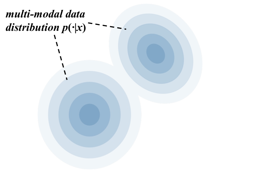
(a)

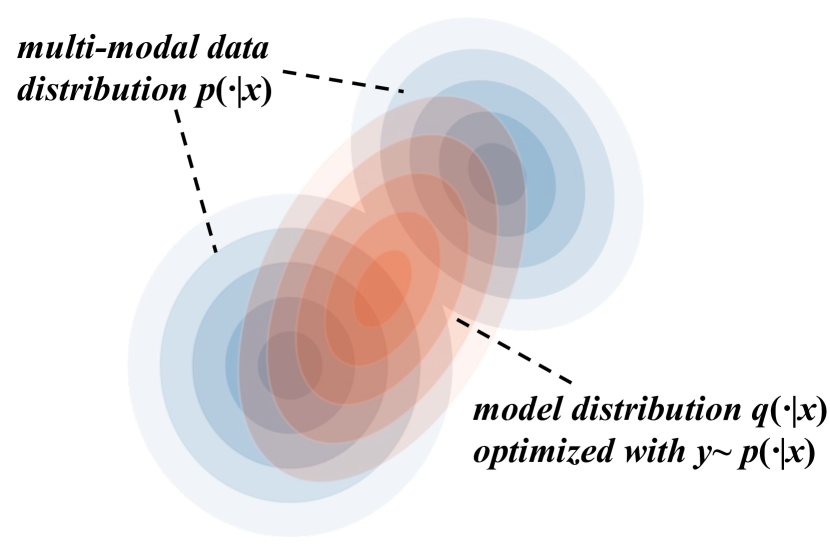
(b)

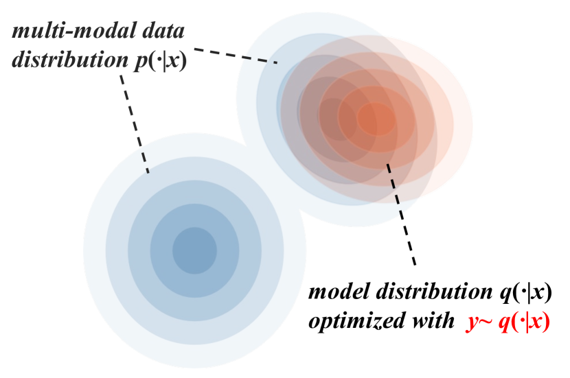
(c)

Figure 1: (a) shows a bimodal data distribution (blue contours). Orange contours in (b) show a single modal model distribution that is optimized to fit the data distribution by samples from the bimodal data distribution. similar to (b), but the model distribution is optimized to a different local minimum with samples from the captured modality of model distribution.

2 Background

Non-autoregressive Generation

Consider predicting a target sequence $\boldsymbol{y}=\{y_{1},y_{2},\ldots,y_{n}\}$ with a source sequence $\boldsymbol{x}=\{x_{1},x_{2},\ldots,x_{m}\}$, where $n$ and $m$ are target and source sequence length respectively. Typical autoregressive transformers model the conditional probability $p(\boldsymbol{y}|\boldsymbol{x})$ via autoregressive decomposition as:

$$p(\boldsymbol{y}|\boldsymbol{x})=\prod_{i=1}^{n}p(y_{i}|y_{<i},\boldsymbol{x}).$$ (1)

While non-autoregressive transformers factorize $p(\boldsymbol{y}|\boldsymbol{x})$ independently with conditional independence assumption:

$$p(\boldsymbol{y}|\boldsymbol{x})=\prod_{i=1}^{n}p(y_{i}|\boldsymbol{x}).$$ (2)

With this assumption, NATs are able to drop the left-to-right dependencies and decode the target sequence in parallel.

DP Training for NATs

The strict position alignment between predicted and target tokens [12, 9] of vanilla NAT has a poor ability to capture the multi-modality data distribution which typically results in generated tokens from mixed modality and repeated words [13]. Dynamic Programming (DP) training [27, 9, 6] greatly alleviate this problem by introducing a long decoder length and alignment-based training objectives that marginalize all the possible alignments that yield the ground-truth. Take the latest work DAT (DA-Transformer) [18] as an example, given the ground truth sequence $\boldsymbol{y}=\{y_{1},y_{2},\ldots,y_{n}\}$ whose length is $n$ and decoder length $L\gg n$, $\mathrm{log}\,q(\boldsymbol{y}|\boldsymbol{x})$ can be defined as:

$$\begin{split}\mathrm{log}\,q(\boldsymbol{y}|\boldsymbol{x})&=\mathrm{log}\,\sum_{\mathbf{a}\in\Gamma}q(\boldsymbol{y},\mathbf{a}|\boldsymbol{x})=\mathrm{log}\,\sum_{\mathbf{a}\in\Gamma}q(\boldsymbol{y}|\mathbf{a},\boldsymbol{x})\cdot q(\mathbf{a}|\boldsymbol{x}),\\ q(\mathbf{a}|\boldsymbol{x})&=\prod_{i=1}^{n-1}\mathbf{E}_{a_{i}.a_{i+1}},\\ q(\boldsymbol{y}|\mathbf{a},\boldsymbol{x})&=\prod_{i=1}^{n}\mathrm{softmax}(\mathbf{W}_{\text{vocab}}\mathbf{h}_{a_{i}}),\end{split}$$ (3)

where $\mathbf{a}$ is a set of decoder position indexes sorted in ascending order whose size $|\mathbf{a}|=n$ and $\Gamma$ contains all possible $\mathbf{a}$ with a size of $\binom{L}{n}$. For example, target length $n=3$ and $L=6$ means $\Gamma$ contains $\binom{6}{3}=20$ possible $\mathbf{a}$, and $\mathbf{a}\in\{0,1,2\},\{0,1,3\}...\{3,4,5\}$. $\mathbf{h}_{a_{i}}$ means the $a_{i}$-th decoder hidden state. $q(\boldsymbol{y}|\mathbf{a},\boldsymbol{x})$ is the token prediction probablity in generation models. $q(\mathbf{a}|\boldsymbol{x})$ is given by the transition matrix $\mathbf{E}\in\mathbb{R}^{L\times L}$ modeling the first-order dependency between decoder position indexes where $\mathbf{E}_{a_{i}.a_{i+1}}$ means the transition probability of index $a_{i}$ to index $a_{j}$ and it is predicted based on the decoder hidden states. Enumerating all $\mathbf{a}\in\Gamma$ will result in the curse of combination, but luckily $\mathbf{E}$ can be trained with the dynamic programming algorithm. Details of the algorithm can be found in Huang et al. [18]. In Figure 4 Appendix, we present an example that highlights 1) the difference between a Dynamic Programming (DP) model and a Vanilla model; 2) the calculation of $q(\mathbf{a}|\boldsymbol{x})$ and $q(\boldsymbol{y}|\mathbf{a},\boldsymbol{x})$. For the decoding procedure, please refer to Appendix E. Training with Dynamic Programming is essential for NATs on raw data; otherwise, their performance lags notably behind that of ATs.

3 Method

3.1 Learning on Model Distribution

Unlike previous efforts that mitigate multi-modality problems via architecture design or decoding algorithm, we attribute the multi-modality problem to the learning objective, maximum likelihood estimation (MLE). MLE minimizes the KL divergence between the data distribution $p(\cdot|\boldsymbol{x})$ and the model distribution $q(\cdot|\boldsymbol{x})$, which can be formulated as follows,

$$\begin{split}\text{KL}(p\parallel q)&=\mathbb{E}_{\boldsymbol{y}\sim p(\cdot|\boldsymbol{x})}[\log\frac{p(\boldsymbol{y}|\boldsymbol{x})}{q(\boldsymbol{y}|\boldsymbol{x})}]\\ &=-H(p)+\mathbb{E}_{\boldsymbol{y}\sim p(\cdot|\boldsymbol{x})}[-\log q(\boldsymbol{y}|\boldsymbol{x})]\end{split}$$ (4)

where $H(p)$ denotes the entropy of data distribution and is a constant. Note that MLE requires sampling from the data distribution $p(\cdot|\boldsymbol{x})$, which forces the NAT model to assign a reasonable probability for each sampled $\boldsymbol{y}$. We argue that this objective could be too difficult for NAT models because of its limited capacity, which may result in low-quality predictions with mixed modalities.

In this work, we suggest that the above problem can be alleviated by replacing the samples from $p(\cdot|\boldsymbol{x})$ with the samples from $q(\cdot|\boldsymbol{x})$, therefore dropping some modalities that are too difficult for NATs to capture. Specifically, we propose a generalized divergence $D(q\parallel p)$ as our objective:

$$\begin{split}D(q\parallel p)&=\mathbb{E}_{\boldsymbol{y}^{\prime}\sim q(\cdot|\boldsymbol{x})}[M_{p,q}(\boldsymbol{y}^{\prime}|\boldsymbol{x})],\end{split}$$ (5)

where $M_{p,q}(\boldsymbol{y}^{\prime}|\boldsymbol{x})$ measures the discrepancy between model and data distribution with a given sample $\boldsymbol{y}^{\prime}$ from the simpler model distribution.

To better explain our intuition, we illustrate an example in Figure 1. In previous objective, $\mathbb{E}_{y\sim p(\cdot|\boldsymbol{x})}[\cdot]$ optimizes samples from all modalities in data distribution $p(\cdot|\boldsymbol{x})$ by assigning them importance rates $p(\boldsymbol{y}|\boldsymbol{x})$, thereby leading to a mixed-modal distribution (see Figure 1(b)); in contrast, $\mathbb{E}_{y^{\prime}\sim q(\cdot|\boldsymbol{x})}[\cdot]$ focuses on samples within a captured modality from modeling distribution $q(\cdot|\boldsymbol{x})$ by assigning low importance rate to uncaptured modalities and keeps on optimizing the captured modalities (see Figure 1(c)). The final training objective is the sum of $\text{KL}(p\parallel q)$ and $\text{D}(q\parallel p)$. $\text{KL}(p\parallel q)$ acts as a regularization to prevent collapse if the samples from model distribution are low-quality.

Our idea is connected to previous work that optimizes reverse KL based on reinforcement learning  [48, 2]. Note that the reverse $\text{KL}(q\parallel p)$ is a special case of Eq. 5, which adopts the discrepancy measure as $\log\frac{q(\boldsymbol{y}^{\prime}|\boldsymbol{x})}{p(\boldsymbol{y}^{\prime}|\boldsymbol{x})}$. However, reinforcement learning necessitates a well-structured parameter space for initialization [5], but in our preliminary experiments, the original KL loss optimized by DP training is easily perturbed by the RL loss that it ultimately impedes performance improvements (see Figure 2(a)). In the next section, we bypass the difficulty of directly optimizing the absolute reward distribution by suggesting more flexible necessary conditions and optimizing the proposed objective contrastively.

3.2 A Contrastive Learning Objective

Having the connection between NATs’ multi-modality challenge and model distribution optimization in the previous discussion, we focus on how to concretize a discrepancy measure $M_{p,q}(\boldsymbol{y}^{\prime}|\boldsymbol{x})$, in a contrastive way, to NAT models. The general methodology is investigating the constraints that are sufficient and necessary to data distribution and then imposing these constraints to model distribution to guide the learning process.

With $\boldsymbol{y}^{\prime}$ sampled from model distribution, it is usually unobserved in the enormous target space, with high probability, in a dataset generated by an unknown distribution. Thus it is untractable to quantify the likelihood $p(\boldsymbol{y}^{\prime}|\boldsymbol{x})$. A practical estimation is to introduce a reward-based distribution $p^{R}(\cdot|\boldsymbol{x},\boldsymbol{y})$, i.e.,

$$p^{R}(\boldsymbol{y}^{\prime}|\boldsymbol{x},\boldsymbol{y})=\frac{1}{Z^{R}}\exp(R(\boldsymbol{y},\boldsymbol{y}^{\prime})),(\boldsymbol{x},\boldsymbol{y})\sim\mathcal{D},$$ (6)

where $R(\cdot,\cdot)$ is a reward function measuring $(\boldsymbol{y},\boldsymbol{y}^{\prime})$’s divergence, and $Z^{R}$ denotes the normalizer. We here use BLEU [34] as a lexical measure for optimization.

We then seek a series of contrastive conditions that are sufficient and necessary to generate the data distribution $p^{R}(\cdot|\boldsymbol{x},\boldsymbol{y})$:

$$\begin{split}\forall\boldsymbol{y}^{\prime}_{+},&\boldsymbol{y}^{\prime}_{-}:\log\frac{p^{R}(\boldsymbol{y}^{\prime}_{+}|\boldsymbol{x},\boldsymbol{y})}{p^{R}(\boldsymbol{y}^{\prime}_{-}|\boldsymbol{x},\boldsymbol{y})}=\epsilon(\boldsymbol{y}^{\prime}_{+},\boldsymbol{y}^{\prime}_{-}|\boldsymbol{y})\\ &\epsilon(\boldsymbol{y}^{\prime}_{+},\boldsymbol{y}^{\prime}_{-}|\boldsymbol{y})=R(\boldsymbol{y}^{\prime}_{+},\boldsymbol{y})-R(\boldsymbol{y}^{\prime}_{-},\boldsymbol{y}),\end{split}$$ (7)

where $\boldsymbol{y}^{\prime}_{+}$ and $\boldsymbol{y}^{\prime}_{-}$ are two samples in target space satisfying $R(\boldsymbol{y}^{\prime}_{+},\boldsymbol{y})>R(\boldsymbol{y}^{\prime}_{-},\boldsymbol{y})$, without loss of generality, and $\epsilon(\boldsymbol{y}^{\prime}_{+},\boldsymbol{y}^{\prime}_{-}|\boldsymbol{y})$ represents $(\boldsymbol{y}^{\prime}_{+},\boldsymbol{y}^{\prime}_{-})$’s reward gap. Detailed proof of necessity and sufficiency is shown in Appendix B. We here focus on its necessity, which is treated as a constraint to model distribution in the future. Consider a bundle of generated sequences $\{\boldsymbol{y}^{\prime}_{k}\sim q(\cdot|\boldsymbol{x})\}_{k=1}^{K}$, satisfying $\forall i>j:R(\boldsymbol{y}^{\prime}_{i},\boldsymbol{y})>R(\boldsymbol{y}^{\prime}_{j},\boldsymbol{y})$, where $K$ is the number of samples. Assuming a small positive lower bound $\epsilon_{\text{LB}}$, namely $\forall i>j:\epsilon(\boldsymbol{y}^{\prime}_{i},\boldsymbol{y}^{\prime}_{j}|\boldsymbol{y})\geq\epsilon_{\text{LB}}$, we have looser necessary conditions pairwisely, as

$$\forall i>j:\log\frac{p^{R}(\boldsymbol{y}^{\prime}_{i}|\boldsymbol{x},\boldsymbol{y})}{p^{R}(\boldsymbol{y}^{\prime}_{j}|\boldsymbol{x},\boldsymbol{y})}\geq\epsilon_{\text{LB}},$$ (8)

where $\epsilon_{\text{LB}}$ is treated as a hyper-parameter. We neglect the event $R(\boldsymbol{y}^{\prime}_{i},\boldsymbol{y})=R(\boldsymbol{y}^{\prime}_{j},\boldsymbol{y})$ whose probability is negligible. By taking $\{\boldsymbol{y}^{\prime}_{j+1},\ldots,\boldsymbol{y}^{\prime}_{i-1}\}$ as intermediate states, we derive stronger necessary conditions,

$$\forall i>j:\log\frac{p^{R}(\boldsymbol{y}^{\prime}_{i}|\boldsymbol{x},\boldsymbol{y})}{p^{R}(\boldsymbol{y}^{\prime}_{j}|\boldsymbol{x},\boldsymbol{y})}\geq(i-j)\epsilon_{\text{LB}},$$ (9)

which is also a ranking-based condition. After all, we impose the conditions in Eq. 9 as constraints to model distribution $q(\cdot|\boldsymbol{x})$, and penalize $q(\cdot|\boldsymbol{x})$ voilating the constraints:

$$\forall i>j:\mathcal{L}_{i,j}=\max\{0,-\log{q(\boldsymbol{y}^{\prime}_{i}|\boldsymbol{x})}+\log{q(\boldsymbol{y}^{\prime}_{j}|\boldsymbol{x})}+(i-j)\epsilon_{\text{LB}}\}.$$ (10)

In typical decomposition-based sequence modeling, $q(\cdot|\boldsymbol{x})$ is heavily biased by sequence length, where shorter ones obtain higher probability and are more favorable [48]. To eliminate the length bias, we normalize $q(\cdot|\boldsymbol{x})$ by the target length $||\boldsymbol{y}^{\prime}||$. In experiments, we implement Eq. 10 by: 1) sampling $K$ hypotheses from the model distribution, 2) constructing $\binom{K}{2}$ pairs, and 3) calculating $\mathcal{L}_{i,j}$ for each pair. Eq. 10 is a contrastive objective, facilitating $M_{p,q}(\cdot|\boldsymbol{x})$ in Eq. 5 by penalizing violated constraints and we show that Eq. 10 can be written with similar form with Eq. 5 in Appendix C, yet it’s crucial to note that they are not strictly equivalent. By optimizing with the contrastive constraints, we show that the original regularization (DP) loss is less likely to obviously increase in Figure 2(b).

3.3 Implementation on NATs

Practical implementation of the contrastive loss includes sampling multiple hypotheses from the model distribution and ranking the likelihood of generated sequences according to some evaluation metrics such as BLEU. The sampling algorithm can be Noisy Parallel Decoding [4, 13] on vanilla NATs which randomly add Gaussian noise to the word embedding layer to generate diverse output, but it involves $sampling\_size$ times additional forward passes consequently leading to increased training costs. Results on vanilla NATs are shown in Table 2. As for DP-based models, sampling positive-negative examples do not obviously bring training cost since the sampling process can be viewed as combining different decoder predictions (See Figure 4 in Appendix) and can be typically implemented by beam search or nucleus sampling [17].

We select previous the best DP-based model DA-Transformer and its pretrained version (for summarization tasks) as our base model in the main experiments considering the following two advantages. i) Accuracy: Samples used to minimize the divergence in Eq.5 are expected to be high-quality and single-modal. In other words, if all training samples are of low quality, the model will be tuned in the wrong direction. Basing on SOTA provides a high-quality sampling space that stabilizes the optimization process and benefits the performance. ii) Efficiency: DA-Transformer is a DP-based model which means sampling multiple hypotheses usually does not involve more cost with the sample size increasing. As mentioned before, DA-Transformer and most DP-based models usually have an extended decoder length to relax the strict alignment between decoder prediction and target words. Actually, sampling hypotheses from DP-based models is equivalent to combing the predicted words from different decoder positions, which means a generated sequence (length<$L$) is a subset of words from all $L$ predicted words (see the example in Figure 4 Appendix) without more floating point operations or forward passes (see Appendix E).

In experiments, we find the process of contrasting low-likelihood sequences adversely has a negative effect on the original DP training loss, resulting in instability and unsatisfied results during training. In order to avoid training on such samples, we adopt two filtering tricks: 1) hypotheses-level filtering: sampling a larger amount of hypotheses first and then keeping only the top 25% for training. 2) Samples-level filtering: some challenging training samples may exhibit significantly low sequence likelihood on target from data distribution and usually have low-quality sampling space. Persisting in optimizing on these samples with model generated sequences will ultimately result in poor performance (in both reinforcement learning and contrastive learning setting). Therefore, we exclude training samples with DP training loss exceeding $\alpha$ when optimizing the discrepancy $M_{p,q}(\boldsymbol{y}^{\prime}|\boldsymbol{x})$ with target sequences from the model distribution. $\alpha$ is practically set to the value of $\mathbb{E}_{\boldsymbol{y}\sim\mathcal{V}}[-\log q(\boldsymbol{y}|\boldsymbol{x})]$ where $\mathcal{V}$ means the validation set.

4 Experiments

We verify CoDAT on three different text generation tasks, including machine translation, summarization, and paraphrasing, with five different benchmarks. We show that the results of non-autoregressive Transformers can be boosted to a new level with the contrastive learning framework. Particularly, we exceed the autoregressive Transformer on the two summarization datasets and achieve an improvement of 0.83 BLEU score on average on the translation datasets and paraphrase dataset. Training details and hyperparameters can be found in Appendix D

4.1 Quantitative Results

This section shows the results of CoDAT on serval mainstream text generation benchmarks. To prove our method has a stronger modality learning ability, we directly use the raw dataset for machine translation and paraphrasing. We use distillation data for summarization following previous work. We use the most standard evaluation metrics for each task in our main results.

Machine Translation

For machine translation, we evaluate CoDAT on WMT14 English $\leftrightarrow$ German translation task (4M samples), WMT17 English $\leftrightarrow$ Chinese translation task (20M samples) and follow the default split of test and validation set of FairSeq [33]. We evaluate our model on all datasets with tokenized BLEU except WMT17 En$\rightarrow$Zh, which is assessed with SacreBLEU [35]. We also reproduce the autoregressive Transformer and DA-Transformer (DAT) with the same running environment as CoDAT. Since previously reported results is trained with 100k steps and a batch size of 32k tokens, our implementation achieves higher performance. The main results are shown in Table 1. Among all iterative NATs and fully NATs, our method CoDAT achieves the best result and outperforms previous state-of-the-art by a remarkable margin. The average performance gap between the autoregressive transformer and non-autoregressive transformer is reduced to 0.4 with our contrastive learning method. We also show that directly optimizing the reward can also bring improvements to the original DAT. However, due to its negative impact on the original training loss, optimizing the constraints usually brings higher performance. All the hypotheses are sampled from the model distribution in parallel without normalizing and selecting at each step like the beam search algorithm. Therefore, it still maintains a 10.2 times speedup during inference with only native PyTorch operations.

Table 1: BLEU scores on WMT14 En$\leftrightarrow$De, WMT17 Zh$\leftrightarrow$En translation tasks. The results of previous NATs are quoted from their papers and Huang et al. [18]. +Reward means we optimize the reward distribution derived from Eq. 5 and +Constraints means we optimize the contrastive objective. The best results for NATs are in bold.

Model	Iter.	Speedup	WMT14		WMT17
			En-De	De-En	En-Zh	Zh-En
Transformer [46]	$N$	1.0x	27.6	31.4	34.3	23.7
Transformer (Ours)	$N$	1.0x	27.85	31.64	34.89	23.72
CMLM [7]	10	2.2x	24.61	29.40	–	–
SMART [10]	10	2.2x	25.10	29.58	–	–
DisCo [22]	$\approx 4$	3.5x	25.64	–	–	–
Imputer [39]	8	2.7x	25.0	–	–	–
CMLMC [20]	10	1.7x	26.40	30.92	–	–
Vanilla NAT [12]	1	15.3x	11.79	16.27	18.92	8.69
AXE  [9]	1	14.2x	20.40	24.90	–	–
OaXE [6]	1	14.2x	22.4	26.8	–	–
CTC [27]	1	14.6x	18.42	23.65	26.84	12.23
GLAT [37]	1	15.3x	19.42	26.51	29.79	18.88
CTC + GLAT [37]	1	14.2x	25.02	29.14	30.65	19.92
DAT [18]	1	13.9x	26.57	30.68	33.83	22.82
DAT+Viterbi [41]	1	13.2x	26.89	31.10	33.65	23.24
DAT (Ours)	1	13.9x	26.63	30.73	33.56	22.68
+ Reward	1	10.2x	27.06	31.22	33.59	23.16
+ Constraints	1	10.2x	27.40	31.64	34.23	23.71

Paraphrase

For paraphrase, we adopt the Quora Question Pairs (QQP) collected from the Quora community question answering forum with 147 training pairs. We evaluate generated results with BLEU and ROUGE-L. The performance gap between CoDAT and the autoregressive baseline is reduced to 0.02 BLEU and we even get 0.6 improvements over the autoregressive model in terms of ROUGE-L.

Table 2: Results on the WMT14 en-de benchmark of vanilla model GLAT and DP-based model DAT with different training objectives: MLE, Reward, and Constraints. For GLAT, directly optimizing the reward distribution also yields satisfactory results, but for DAT, optimizing using constraints usually leads to better performance. We use the NPD size = 7.

Model	Dataset	Objective	BLEU
GLAT	Raw	$\text{D}(p\parallel q)$	19.42
GLAT	KD	$\text{D}(p\parallel q)$	25.28
GLAT	KD	$\text{D}(q\parallel p)$ (Reward)	25.71
GLAT	KD	$\text{D}(q\parallel p)$(Constraints)	25.66
DAT	Raw	$\text{D}(p\parallel q)$	26.63
DAT	Raw	$\text{D}(q\parallel p)$ (Reward)	27.06
DAT	Raw	$\text{D}(q\parallel p)$(Constraints)	27.40

Table 3: Results on the test set of QQP in terms of BLEU and ROUGE-L. Results with $*$ are from Gong et al. [11]. The best results of NAT are in bold. CoDAT has $\sim$6.8$\times$ speedup compared with the autoregressive model.

Model	BLEU	ROUGE-L
GRU-attention∗	18.94	51.29
Transformer	27.80	57.94
LevT [14]∗	22.68	57.95
GLAT [37]	25.16	58.28
DiffuSeq [11]∗	24.13	58.80
DAT [18]	27.00	58.31
CoDAT	27.78	58.54

Summarization

For summarization, we achieve new state-of-the-art for NATs on two widely-used news summarization datasets XSum [32] and Gigaword [38]. Gigaword has 4M article-headline pairs and XSum has 227k articles with human-written summaries from BBC News. We use ROUGE [28] as the evaluation metric. To have a fair comparison with previous work, we also perform knowledge distillation before training. Table 4 shows the ROUGE scores on Summarization datasets. Similar to machine translation, we also implement an autoregressive Transformer with the same running environment e.g., the same knowledge distillation dataset and training steps. CoDAT surpasses the autoregressive baselines on both XSum and Gigaword. Generally, CoDAT improves DAT by more than 0.5 ROUGE-1 score and improves the pretrained version of DAT by 1.07 ROUGE-1 score. On XSum, CoDAT without pretraining obtains on-par performance with BANG [36] which is pretrained on large-scale unlabeled corpus and exceeds BANG by 2.44 ROUGE-2. CoDAT achieves a speedup ratio of $\sim 8.4\times$ on XSum and $\sim 6.0\times$ on Gigaword compared with the autoregressive basline. In addition, we also validate our method by building on the strong pretrained version of DAT [19]. Results show that CoDAT (pretrained) even exceeds many strong pretrained AT baselines on XSum.

Table 4: ROUGE scores on Summarization datasets. Avg means the average of ROUGE-1, ROUGE-2 and ROUGE-L. Results with ^† are token from Su et al. [42] and results with ^∗ are from Qi et al. [36]. Results that exceed the autoregressive model are underlined (w/o pretrained), and the best results of NAT are in bold. CoDAT accelerates the autoregressive model by $\sim$8.4 times on XSum and $\sim$6.0 times on Gigaword. The third block contains results of pretrained baselines.

Model	XSum				Gigaword
	R-1	R-2	R-L	Avg	R-1	R-2	R-L	Avg
Transformer [46]	30.66	10.80	24.48	22.0	35.74	16.97	33.43	28.7
Transformer (Ours)	32.07	11.31	25.96	23.1	36.99	18.22	34.48	29.9
Vanilla NAT [12]∗	24.04	3.88	20.32	16.1	27.20	8.96	25.58	20.6
LevT [14]	24.75	4.18	20.87	16.6	30.40	11.89	29.56	23.9
CMLM [20]∗	23.82	3.60	20.15	15.8	–	–	–	–
NART-CRF [45]†	–	–	–	–	30.29	12.61	28.71	23.9
BERT-NAG [42]†	–	–	–	–	35.05	16.48	33.28	28.3
DAT [18]	31.87	11.02	25.93	22.9	36.52	17.94	34.30	29.6
BANG [36]∗	32.59	8.98	27.41	23.0	–	–	–	–
MIST [21]	34.63	11.29	28.70	24.9	–	–	–	–
DAT (Pretrained) [19]	38.80	16.07	31.78	28.9	36.15	17.49	33.84	29.2
CoDAT	32.45	11.42	26.30	23.4	37.01	18.68	34.63	30.1
CoDAT (Pretrained)	39.87	17.38	32.61	30.0	36.92	18.23	34.46	29.9

4.2 Discussion

Ground truth:	According to the proposal, parking fees are to be increased by 50 percent.
3 outputs from DAT	1. There is an increase in parking charges should be increased by 50 %.
	2. The proposed increase in parking charges should therefore be increased by 50 %.
	3. Accordingly, the increase in parking charges are to be increased by 50 %.
3 outputs from CoDAT	1.The proposal is that parking charges should therefore be increased by 50 %.
	2. According to it, the parking charges should be increased by 50% .
	3. According to it, there will be increase in parking charges should be increased by 50 % .

Table 5: An example from WMT14 De$\rightarrow$En translation. We adopt a Sampling size = 128 and present the top 3 hypotheses from DAT and CoDAT. Given the input German $\boldsymbol{x}=$"Demnach sollen die Parkgebühren um 50 Prozent erhöht werden ." Though, the first-order dependency introduced by DAT effectively reduces repeated words, it still can not prevent the generated sequence mixing words from several possible translations while the rank of single-modal translation is higher in the sampling results of CoDAT

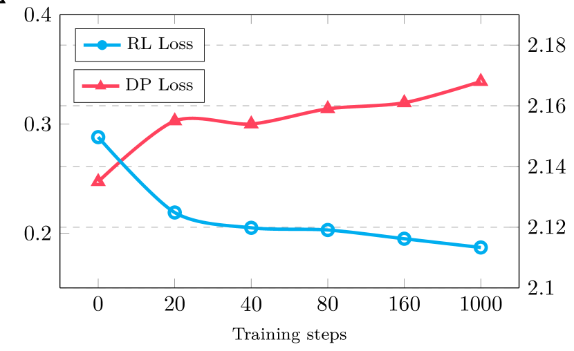
(a) Reinforcement Learning (RL) loss and DP Loss on the validation set of WMT14 en-de benchmark. The left Y-axis represents the value of RL loss, while the right Y-axis corresponds to the value of DP loss.

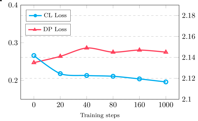
(b) Contrastive Learning (CL) loss and DP Loss on the validation set of WMT14 en-de benchmark. The left Y-axis represents the value of CL loss, while the right Y-axis corresponds to the value of DP loss.

Reducing Data Modality

Normalized Corpus-level Multimodality(NCM) [44] is a metric for measuring corpus-level multimodality for NATs (the lower, the better). Given a translation dataset $\mathcal{D}$ we have the NCM as: $\frac{\mathbb{E}_{(\boldsymbol{x},\boldsymbol{y})\sim\mathcal{D}}[-\log p(\boldsymbol{y}|\boldsymbol{x})]}{\mathbb{E}_{\boldsymbol{y}\sim\mathcal{D}}[\boldsymbol{|\boldsymbol{y}|}]}$. A non-autoregressive model concurrently considering numerous potential translations, it tends to distribute excess probability across different sequences. As a result, it ends up creating translations that are less likely. We validate the NCM of CoDAT and DAT on WMT14 En$\rightarrow$De and De$\rightarrow$En translation task. Results show that we reduce the NCM of DAT from 0.86 to 0.72 on En$\rightarrow$De translation and from 0.91 to 0.79 on De$\rightarrow$En.

But there is no widely accepted metric for modality learning of NATs, we also provide a case study from WMT14 De$\rightarrow$En in Table 5 to showcase that the first-order dependency DP loss can not guarantee generated texts are single modal. The top-3 hypotheses sampled from DAT in Table 5 are all mixed modal translations. For example, the first hypothesis from DAT is a mixed translation of "There is a 50% increase in parking charges" and "parking charges should be increased by 50%" due to “charges” and “should” are very likely to appear together in the training corpus so that they will be assigned a high transition score. But mixing words and phrases from the two modalities will always result in a bad translation while evaluating. We show that the problem can be alleviated via training with contrastive constraints which improves the ranking of high-quality and single-modal hypotheses (there is only 1 translation mixing words from different modalities results).

Scaling with Decoder Length and Sampling Size

We further examine how the decoder length of DAT affects our method. Notice that a longer decoder length often provides an enlarged sampling space. We vary the decoder length from 128 to 1,024 and measure the performance gap between CoDAT and DAT according to BLEU on the test set of WMT14 En$\rightarrow$De translation task. Results are shown in Figure 3(b), when we have a decoder length longer than 384, CoDAT generally has an improvement of more than 0.5 BLEU. CoDAT (decoder length = 384) realizes on-par performance with DAT (decoder length = 1024). However, when the decoder length is set to a smaller value of 256, the improvement seems marginal. Recalling that CoDAT advocates modality learning by optimizing $D(q\parallel p)$ with samples from model distribution $\boldsymbol{y}^{\prime}\sim q(\cdot|\boldsymbol{x})$. We attribute the low performance of CoDAT to the reduced sampling space when with a short decoder length. We measure the sampling space with a heuristic method: BLEU of the best sample. We respectively calculate the best result among the decoded 64 samples (named Oracle BLEU) with decoder lengths set to 256 and 512. The longer length achieves 34.12 Oracle BLEU while the shorter length only achieves 30.28 Oracle BLEU. The performance gap indicates the size of the sampling space plays an important role in our method. We further examine the performance of CoDAT with sampling size. With the increase in sampling size, single-modal translations also have a higher probability of appearing in the sampling space. According to our training objective, their ranking in the sampled outputs will be elevated, thus improving the model’s performance.

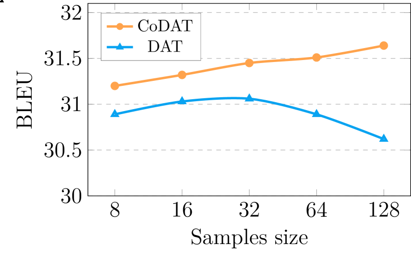
(a) Test BLEU score with the sample size on WMT14 De$\rightarrow$En translation. We use the size of generated samples as the X-axis and the Y-axis represents the BLEU score.

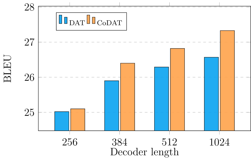
(b) Test BLEU score of CoDAT and DAT with the decoder length on WMT14 En$\rightarrow$De translation. We use the decoder length as the X-axis and the Y-axis represents the BLEU score.

5 Related work

Non-autoregressive Text Generation

Non-autoregressive text generation is originally developed in machine translations [12, 16]. Gu et al. [12] design the first NAT model that decodes the whole sequence in parallel. Fully NATs predict the sequence with only one forward pass. Compared with fully NATs, iterative NATs [24, 15, 7, 16] repeatedly refine the prediction by iterative decoding. Iterative NATs usually achieve better performance but trade efficiency for accuracy. As introduced in the background, non-iterative NATs are greatly improved by DP training [27, 9, 18] which abandons the position-wise alignment of Vanilla NAT and allows flexible length. Based on DAT, the latest work FDAT [31] introduces fuzzy alignment for DAT and greatly improves the performance on translation tasks but sacrifices the generation diversity. Non-autoregressive models are also introduced in other areas. Wiseman et al. [47] propose a hidden semi-Markov model for data-to-text generation. BANG [36] and MIST [21] are pretraining frameworks for NAT models. Su et al. [42], Sun et al. [45] successfully utilize pre-trained encoder BERT and a conditional random field (CRF) to non-autoregressive summarization and machine translation. Most NATs strongly depend on sentence-level knowledge distillation [13] datasets. This requires pretraining an autoregressive model to generate the training set but is very useful to reduce the data modality [50].

Contrastive Learning for Text Generation

The triplet loss used in this work is originally proposed in faceNet [40], aiming to learn a good representation via contrasting positives to negatives. Contrastive learning has also been widely used in autoregressive text generation [25, 1, 26] and summarization [29, 43], and to the best of our knowledge, we are the first contrastive learning framework in non-autoregressive generation. In the field of text summarization, Zhong et al. [49] propose contrastive learning to model that the document and its summary should be close in the embedding space. Previous work on autoregressive generation [25, 30, 1] shares a common motivation: mitigating the exposure bias problem. The contrastive loss we used in training has a similar format to the training objective of previous autoregressive models BRIO [30] and CoNT [1]. Our work differs from theirs in two aspects. 1) Different settings: our method is based on the setting of DP-based non-autoregressive models which has a very different input space and training process compared with the autoregressive model. 2) Different motivations: we hold the motivation of helping the modality learning of NATs and our contrastive objective is derived from seeking contrastive constraints while they hold the motivation from exposure bias and learning fine-gained representations.

6 Conclusion

In this paper, we develop the first contrastive learning framework for non-autoregressive generation. The goal of our contrastive learning objective is alleviating the modality learning of NATs by using training samples from the model distribution instead of complex data distribution. In order to stabilize training, we derive contrastive constraints which finally lead to a contrastive learning loss. Experiments on three text generation tasks demonstrate that our method achieves the best results on all these tasks for non-autoregressive models. Our work has many limitations please refer to Appendix F for details.

Appendix A Reverse KL and Reinforcement Learning

Above all, we treat $p(\boldsymbol{y}|\boldsymbol{x})$ as Eq. 6.

$$\;\;\;\;\text{KL}(q\parallel p)$$

$$=\mathbb{E}_{\boldsymbol{y}^{\prime}\sim q(\cdot|\boldsymbol{x})}[\log\frac{q(\boldsymbol{y}^{\prime}|\boldsymbol{x})}{p(\boldsymbol{y}^{\prime}|\boldsymbol{x})}]$$

$$=\mathbb{E}_{\boldsymbol{y}^{\prime}\sim q(\cdot|\boldsymbol{x})}[\log q(\boldsymbol{y}^{\prime}|\boldsymbol{x})-R(\boldsymbol{y},\boldsymbol{y}^{\prime})+\log Z^{R}]$$

$$=-H(q)-\mathbb{E}_{\boldsymbol{y}^{\prime}\sim q(\cdot|\boldsymbol{x})}[R(\boldsymbol{y},\boldsymbol{y}^{\prime})-\log Z^{R}]$$

where $H(q)$ is the entropy of model distribution, $\mathbb{E}_{\boldsymbol{y}\sim q(\cdot|\boldsymbol{x})}[R(\boldsymbol{y},\boldsymbol{y}^{\prime})-\log Z^{R}]$ is reinforcement learning with a normalized reward. Thus minimizing $\text{KL}(q\parallel p)$ implicitly maximizes rewards on model distribution.

Appendix B Sufficiency & Necessity

Proposition B.1.

For any sequence pair $\boldsymbol{y}\textquoteright_{1},\boldsymbol{y}^{\prime}_{2}$, $\boldsymbol{y}\textquoteright_{1},\boldsymbol{y}^{\prime}_{2}\sim p^{R}(\boldsymbol{y}^{\prime}|\mathbf{x},\boldsymbol{y})=\frac{1}{Z^{R}}\exp(R(\boldsymbol{y},\boldsymbol{y}^{\prime}))$ is sufficient and necessary to $\log\frac{p^{R}(\boldsymbol{y}^{\prime}_{1}|\mathbf{x},\boldsymbol{y})}{p^{R}(\boldsymbol{y}^{\prime}_{2}|\mathbf{x},\boldsymbol{y})}=R(\boldsymbol{y}^{\prime}_{1},\boldsymbol{y})-R(\boldsymbol{y}^{\prime}_{2},\boldsymbol{y})$.

Proof.

We prove the sufficiency and necessity individually as follows:

(Sufficiency)

$$\forall\boldsymbol{y}\textquoteright_{1},\boldsymbol{y}^{\prime}_{2}:\log\frac{p^{R}(\boldsymbol{y}^{\prime}_{1}|\mathbf{x},\boldsymbol{y})}{p^{R}(\boldsymbol{y}^{\prime}_{2}|\mathbf{x},\boldsymbol{y})}=R(\boldsymbol{y}^{\prime}_{1},\boldsymbol{y})-R(\boldsymbol{y}^{\prime}_{2},\boldsymbol{y})$$

$$\forall\boldsymbol{y}\textquoteright_{1},\boldsymbol{y}^{\prime}_{2}:\log p^{R}(\boldsymbol{y}^{\prime}_{1}|\mathbf{x},\boldsymbol{y})-R(\boldsymbol{y}^{\prime}_{1})\quad\quad\quad\quad\quad\quad$$

$$=\log p^{R}(\boldsymbol{y}^{\prime}_{2}|\mathbf{x},\boldsymbol{y})-R(\boldsymbol{y}^{\prime}_{2})$$

Without loss of generality, we set the difference at both side to a constant $C$

$$\forall\boldsymbol{y}^{\prime}:\log p^{R}(\boldsymbol{y}^{\prime}|\mathbf{x},\boldsymbol{y})-R(\boldsymbol{y}^{\prime})=C$$

Thus

$$\forall\boldsymbol{y}^{\prime}:p^{R}(\boldsymbol{y}^{\prime}|\mathbf{x},\boldsymbol{y})=\exp(C)\exp(R(\boldsymbol{y},\boldsymbol{y}^{\prime}))$$

By rewriting this into a normalization form, we have

$$\forall\boldsymbol{y}^{\prime}:p^{R}(\boldsymbol{y}^{\prime}|\mathbf{x},\boldsymbol{y})=\frac{1}{Z^{R}}\exp(R(\boldsymbol{y},\boldsymbol{y}^{\prime}))$$

where $Z^{R}=1/\exp(C)$.

(Necessity) The necessity is quite straightforward by directly replacing $p^{R}(\boldsymbol{y}^{\prime}_{1}|\mathbf{x},\boldsymbol{y})=\frac{1}{Z^{R}}\exp(R(\boldsymbol{y},\boldsymbol{y}^{\prime}_{2}))$ and $p^{R}(\boldsymbol{y}^{\prime}_{2}|\mathbf{x},\boldsymbol{y})=\frac{1}{Z^{R}}\exp(R(\boldsymbol{y},\boldsymbol{y}^{\prime}_{2}))$ into $\log\frac{p^{R}(\boldsymbol{y}^{\prime}_{1}|\mathbf{x},\boldsymbol{y})}{p^{R}(\boldsymbol{y}^{\prime}_{2}|\mathbf{x},\boldsymbol{y})}$.

∎

Appendix C Contrastive Discrepancy

The original Eq. 5 can be rewritten to:

$$\mathrm{KL}(q\parallel p)=\mathbb{E}_{\boldsymbol{x},\boldsymbol{y}\sim\mathcal{D},\boldsymbol{y}^{\prime}\sim q(\cdot|\boldsymbol{x})}[M_{p,q}(\boldsymbol{y}^{\prime}|\boldsymbol{x})]$$

$$=\mathbb{E}_{\boldsymbol{x},\boldsymbol{y}\sim\mathcal{D},\{\boldsymbol{y}^{\prime}_{k}\}_{k=1}^{K}\sim q(\cdot|\boldsymbol{x})}[\frac{1}{K}\sum_{k}M_{p,q}(\boldsymbol{y}^{\prime}_{k}|\boldsymbol{x})].$$

We can also understand the contrastive loss from the perspective of the relative version of the reverse KL loss in original Eq. 5. let $[\boldsymbol{y}^{\prime}_{i},\boldsymbol{y}^{\prime}_{j}]$ denote the difference between a sequence pair from the model distribution, and $\boldsymbol{y}$ is from the data distribution. If there is a significant disparity in the data distribution of the two samples, we will also expect a commensurate divergence in their respective model distribution. $M_{p,q}([\boldsymbol{y}^{\prime}_{i},\boldsymbol{y}^{\prime}_{j}]|\boldsymbol{x}))]$ measures the discrepancy between model and data distribution given the difference of the pair instead of directly optimizing with only one sample like the original Eq. 5. We can estimate $p([\boldsymbol{y}^{\prime}_{i},\boldsymbol{y}^{\prime}_{j}]|\boldsymbol{x})$ with a reward distribution: $\frac{1}{Z_{1}}\cdot\frac{e^{R(\boldsymbol{y}^{\prime}_{i},\boldsymbol{y})}}{e^{R(\boldsymbol{y}^{\prime}_{j},\boldsymbol{y})}}$ and $q([\boldsymbol{y}^{\prime}_{i},\boldsymbol{y}^{\prime}_{j}]|\boldsymbol{x})$ with $\frac{1}{Z_{2}}\cdot\frac{q(\boldsymbol{y}^{\prime}_{i}|\boldsymbol{x})}{q(\boldsymbol{y}^{\prime}_{j}|\boldsymbol{x})}$ where $Z_{1}$ and $Z_{2}$ are normalizing constants. By optimizing $M_{p,q}([\boldsymbol{y}^{\prime}_{i},\boldsymbol{y}^{\prime}_{j}]|\boldsymbol{x}))]$, the Eq. 10 also has a similar form with Eq. 5:

$$\mathbb{E}_{\boldsymbol{x},\boldsymbol{y}\sim\mathcal{D},\{\boldsymbol{y}^{\prime}_{k}\}_{k=1}^{K}\sim q(\cdot|\boldsymbol{x})}[\frac{2}{K(K-1)}\sum_{i>j}M_{p,q}([\boldsymbol{y}^{\prime}_{i},\boldsymbol{y}^{\prime}_{j}]|\boldsymbol{x})]$$

$$= \mathbb{E}_{\boldsymbol{x},\boldsymbol{y}\sim\mathcal{D},\{\boldsymbol{y}^{\prime}_{k}\}_{k=1}^{K}\sim q(\cdot|\boldsymbol{x})}[\frac{2}{K(K-1)}\sum_{i>j}\log\frac{p([\boldsymbol{y}^{\prime}_{i},\boldsymbol{y}^{\prime}_{j}]|\boldsymbol{x})}{q([\boldsymbol{y}^{\prime}_{i},\boldsymbol{y}^{\prime}_{j}]|\boldsymbol{x})}]$$

$$\approx \mathbb{E}_{\boldsymbol{x},\boldsymbol{y}\sim\mathcal{D},\{\boldsymbol{y}^{\prime}_{k}\}_{k=1}^{K}\sim q(\cdot|\boldsymbol{x})}[\frac{2}{K(K-1)}\sum_{i>j}\max\{0,$$

$$\;\;\;\;\;\;\;\;-\log q(\boldsymbol{y}^{\prime}_{i}|\boldsymbol{x})+\log q(\boldsymbol{y}^{\prime}_{j}|\boldsymbol{x})+(i-j)\epsilon_{\text{LB}}\}]$$

Appendix D Experimental Setup

Implementation

In order to sample meaningful positive and negative examples, we first warmup DA-Transformer with the DP loss shown in Eq. 3. In the warmup stage, we follow the default settings of the open source implementation of DA-Transformer. The learning rate for the machine translation task is set to $5\times 10^{-4}$ but for summarization and paraphrasing, we use a smaller learning rate $1\times 10^{-4}$. Excluding contrastive learning, we also apply DP training and glancing to help reduce the multi-modality of data distribution. For glancing, we linearly decrease the unmasking ratio from 0.5 to 0.1 until the training steps = 200k. For DP training, we extend the decoder length to 8 times of the encoder length. We set the margin value $\epsilon_{\text{LB}}$ to 0.001. The sampling size in both training and inference is 128 and we only keep the 25% for training. We set the sampling temperature $\tau$ to 0.1 during training and $0.05$ during inference. The contrastive loss and DP loss are optimized with the same Adam optimizer [23]. We use a batch size of 256k tokens by reducing the frequency of gradient updates to stabilize the training process. After pretraining the model for 120 epochs with DP loss, we further train the model for 5 epochs with the sum of DP loss and contrastive loss. Our code base is built on fairseq [33] toolkit. It takes about 1 hour on 4 NVIDIA Tesla A100 GPUs for contrastive optimization on the XSum summarization dataset and 4 hours for the large-scale WMT14 En-De translation task. We assess BLEU on the validation set every 40 steps, and then the top 5 checkpoints are saved and averaged to produce the result on the test set. We use the base version of Transformer [46] with 6 encoders and 6 decoders as the autoregressive baseline. The decoding speedup is tested with the batch size set to 1 following previous work on single A100 GPU and we report the average speedup of three runs. We calculate ROUGE with the pyrouge library. Both the tokenized BLEU and sacreBLEU are calculated with fairseq. During decoding, We use the sampling algorithm to derive multiple hypotheses from the model by Algorithm 2. We decompose the sequence probability into transition score ($q(\mathbf{a}|\boldsymbol{x})$) and prediction score ($q(\boldsymbol{y}|\boldsymbol{x},\mathbf{a})$). the sequence score is given by: $\beta\cdot q(\boldsymbol{y}|\boldsymbol{x},\mathbf{a})+(1-\beta)\cdot q(\mathbf{a}|\boldsymbol{x})$ where beta is a hyperparameter tuned on the validation set. We tune $\beta$ from [0.3, 0.5, 0.7]. The validation loss for the checkpoint we used for WMT14 En-De translation is 2.134, so we set $\alpha$ to 2.1 which means training samples with DP Loss larger than 2.1 will not be optimized with samples from the model distribution for stability.

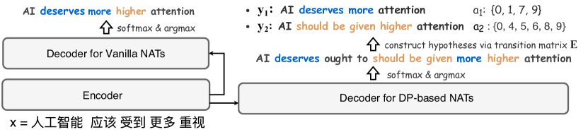
Figure 4: Comparasion of Vanilla NATs and DP-based NATs. The input/output length of Vanilla NATs is usually predicted by the model, and the prediction from each position is directly taken as model output. While the decoder length of DP-based models such as CTC [27] and DAT [18] is a hyperparameter (usually set as 2x$\sim$8x encoder length). For DAT, the decoder first predicts a word from each position, and the hypothesis is a subset of all predicted words constructed via the transition matrix. Given a hypothesis $\boldsymbol{y}_{1}$ from positions $\mathbf{a_{1}}=\{0,1,7,9\}$, $q(\mathbf{a_{1}}|\boldsymbol{x})$ is calculated as $\mathbf{E}_{0,1}\cdot\mathbf{E}_{1,7}\cdot\mathbf{E}_{7,9}$ and $q(\boldsymbol{y_{1}}|\mathbf{a_{1}},\boldsymbol{x})$ is the product of the corresponding token probability $p(\texttt{`AI'}|0,\boldsymbol{x})\cdot p(\texttt{`deserves'}|1,\boldsymbol{x})\cdot p(\texttt{`more'}|7,\boldsymbol{x})\cdot p(\texttt{`attention'}|9,\boldsymbol{x})$.

Appendix E Details of DAT Inference

Latest work CTC [27] and DA-Transformer [18] adopt a Dynamic Programming (DP) training framework significantly improving WMT14 en-de translation benchmark by $4\sim 5$ BLEU.

In this part, we present a concrete demonstration to perform sampling on DA-Transformer. Given the decoder length $L$ and decoder hidden states $\mathbf{H}=\{\mathbf{h}_{0},\mathbf{h}_{1},\ldots,\mathbf{h}_{L}\}$, we can get the token prediction distribution by: $\mathrm{softmax}(\mathbf{W}_{vocab}\mathbf{H})$ and the $L$ predicted tokens by argmax function.

Figure 4 is a specific case when $L=10$. Notably, the $L$ words can not be viewed as the final output in DAT. Compared with vanilla NAT, a hypothesis in DA-Transformer is represented as a small subset of the $L$ predicted tokens which means sampling hypotheses is equivalent to combining different tokens from the model’s prediction. Notably, this can be done efficiently without any additional forward passes. Sampling a subset from these predictions usually depends on the transition matrix $\mathbf{E}\in\mathbb{R}^{L\times L}$ trained with the DP loss in Eq. 3 where $\mathbf{E}_{ij}$ means the transition probability between position $i$ and $j$. Every hypothesis from DAT starts from position 0 and the next token depends on $\arg\max(\mathbf{E}_{[0,:]})$, and the generation process stops when decoding the ‘<eos>’ token. This is the simplest version of decoding in DAT. The commonly used decoding algorithm in DAT is called lookahead. Details of the algorithm are shown in Algorithm 1. By replacing the $\arg\max$ function with multinomial sampling, we can get diverse output parallelly (see Algorithm 2).

Algorithm 1 Given decoder length $L$, transition matrix $\mathbf{E}\in\mathbb{R}^{L\times L}$ and the token probability vector $\mathbf{t}\in\mathbb{R}^{L}$; return decoder indexes of the output

1:procedure Lookahead

2:    $\mathbf{P}$ = $\mathbf{E}$ + $\mathbf{t}$.unsqueeze(dim=0) $\triangleright$ consider both transition probability and prediction probability

3:    $i:=1$, output := Zeros [max_step]

4:    repeat

5:        dist := $\mathbf{P}$ [outputs[$i-1$]] $\triangleright$ get the distribution of current step given the previous step output

6:        output[$i$] := argmax(dist)

7:    until $i$ = max_step;

8:    return output

Algorithm 2 Given decoder length $L$, temperature $\tau$, transition matrix $\mathbf{E}\in\mathbb{R}^{L\times L}$ and the token probability vector $\mathbf{t}\in\mathbb{R}^{L}$; return decoder indexes of the output

1:procedure SAMPLING

2:    $\mathbf{t}$ = $\mathbf{t}$ / sum($\mathbf{t}$)

3:    $\mathbf{P}$ = $\mathbf{E}$ + $\mathbf{t}$.unsqueeze(dim=0)

4:    $\mathbf{P}$ = Topp_Filter( $\mathbf{P}$, $p=0.5$) $\triangleright$ skip positions with low probability

5:    $\mathbf{P}$ = SoftMax( $\mathbf{P}$ / $\tau$, dim=1) $\triangleright$ re-normalize after filtering

6:    $i:=1$, output := Zeros [max_step]

7:    repeat

8:        dist := $\mathbf{P}$ [outputs[$i-1$]] $\triangleright$ get the distribution of current step given the previous step output

9:        output[$i$] := Multinomial(dist, num=1)

10:    until $i$ = max_step;

11:    return output

Appendix F Limitations

We summarize our limitations from three aspects. Firstly, the performance increase brought by contrastive learning-based training is closely related to the ability of the backbone model. The base model should generate a set of diverse hypotheses and contains high-quality and single-modal samples which can be measured with Oracle BLEU. This limits our contrastive training procedure from directly starting from a random initialized model distribution, and it needs the parameters of the model distribution to have been previously trained to a good parameter space that can provide high-quality samples. Considering the training samples of contrastive loss are from the model distribution instead of data distribution the improvements over strong baselines (especially for the pretrained model) are usually more remarkable.

Secondly, CoDAT also has impacts on the training and inference efficiency. CoDAT needs further training for 5 epochs. Our approach also has a minor impact on inference speed. Since the loss helps the hypothesis with higher bleu have a higher ranking, using sampling algorithms described in Algorithm 2 during inference instead of only decoding one hypothesis usually boosts the performance. During inference, we use a sampling size of 128 and we implement the sampling algorithm with the native torch operations for simplicity.

In practice, using the sampling described in Algorithm 2 is not feasible. Calling torch.MULTINOMIAL every step which is significantly slower than torch.ARGMAX resulting in only a 7.2x speedup ratio compared with the AT counterpart on WMT14 En-De translation task. To omit to call torch.MULTINOMIAL in the loop, we change the algorithm by sampling max_step tokens at each position in parallel and directly obtain the output token instead of sampling every step. Please refer to our updated sampling algorithm Algorithm 3. Despite we have optimized the sampling algorithm numerous times, solely with native torch operations still cannot achieve the same decoding speed as the original DAT that decodes only a single hypothesis.

Algorithm 3 Given decoder length $L$, temperature $\tau$, transition matrix $\mathbf{E}\in\mathbb{R}^{L\times L}$ and the token probability vector $\mathbf{t}\in\mathbb{R}^{L}$; return decoder indexes of the output

1:procedure SAMPLING

2:    $\mathbf{t}$ = $\mathbf{t}$ / sum($\mathbf{t}$)

3:    $\mathbf{P}$ = $\mathbf{E}$ + $\mathbf{t}$.unsqueeze(dim=0)

4:    $\mathbf{P}$ = Topp_Filter( $\mathbf{P}$, $p=0.5$) $\triangleright$ skip positions with low probability

5:    $\mathbf{P}$ = SoftMax( $\mathbf{P}$ / $\tau$, dim=1) $\triangleright$ re-normalize after filtering

6:    $i:=1$, output := Zeros [max_step]

7:    sampled_tokens = Multinomial(P ,max_step) $\triangleright$ shape $L\times$ max_step, sampling max_step tokens at each decoder position

8:    repeat

9:        output[$i$] := sampled_tokens[output[$i-1$]][$i$]

10:    until $i$ = max_step;

11:    return output

References

- An et al. [2022] Chenxin An, Jiangtao Feng, Kai Lv, Lingpeng Kong, Xipeng Qiu, and Xuanjing Huang. CoNT: Contrastive neural text generation. In Alice H. Oh, Alekh Agarwal, Danielle Belgrave, and Kyunghyun Cho, editors, Advances in Neural Information Processing Systems, 2022. URL https://openreview.net/forum?id=mjVZw5ADSbX.
- Bahdanau et al. [2017] Dzmitry Bahdanau, Philemon Brakel, Kelvin Xu, Anirudh Goyal, Ryan Lowe, Joelle Pineau, Aaron Courville, and Yoshua Bengio. An actor-critic algorithm for sequence prediction. In International Conference on Learning Representations, 2017. URL https://openreview.net/forum?id=SJDaqqveg.
- Bishop and Nasrabadi [2006] Christopher M Bishop and Nasser M Nasrabadi. Pattern recognition and machine learning, volume 4. Springer, 2006.
- Cho [2016] Kyunghyun Cho. Noisy parallel approximate decoding for conditional recurrent language model. arXiv preprint arXiv:1605.03835, 2016.
- Choshen et al. [2019] Leshem Choshen, Lior Fox, Zohar Aizenbud, and Omri Abend. On the weaknesses of reinforcement learning for neural machine translation. arXiv preprint arXiv:1907.01752, 2019.
- Du et al. [2021] Cunxiao Du, Zhaopeng Tu, and Jing Jiang. Order-agnostic cross entropy for non-autoregressive machine translation. In Marina Meila and Tong Zhang, editors, Proceedings of the 38th International Conference on Machine Learning, ICML 2021, 18-24 July 2021, Virtual Event, volume 139 of Proceedings of Machine Learning Research, pages 2849–2859. PMLR, 2021. URL http://proceedings.mlr.press/v139/du21c.html.
- Ghazvininejad et al. [2019a] Marjan Ghazvininejad, Omer Levy, Yinhan Liu, and Luke Zettlemoyer. Mask-predict: Parallel decoding of conditional masked language models. In Kentaro Inui, Jing Jiang, Vincent Ng, and Xiaojun Wan, editors, Proceedings of the 2019 Conference on Empirical Methods in Natural Language Processing and the 9th International Joint Conference on Natural Language Processing, EMNLP-IJCNLP 2019, Hong Kong, China, November 3-7, 2019, pages 6111–6120. Association for Computational Linguistics, 2019a. doi: 10.18653/v1/D19-1633. URL https://doi.org/10.18653/v1/D19-1633.
- Ghazvininejad et al. [2019b] Marjan Ghazvininejad, Omer Levy, Yinhan Liu, and Luke Zettlemoyer. Mask-predict: Parallel decoding of conditional masked language models. In Proceedings of the 2019 Conference on Empirical Methods in Natural Language Processing and the 9th International Joint Conference on Natural Language Processing (EMNLP-IJCNLP), pages 6112–6121, Hong Kong, China, November 2019b. Association for Computational Linguistics. doi: 10.18653/v1/D19-1633. URL https://aclanthology.org/D19-1633.
- Ghazvininejad et al. [2020a] Marjan Ghazvininejad, Vladimir Karpukhin, Luke Zettlemoyer, and Omer Levy. Aligned cross entropy for non-autoregressive machine translation. In Proceedings of the 37th International Conference on Machine Learning, ICML 2020, 13-18 July 2020, Virtual Event, volume 119 of Proceedings of Machine Learning Research, pages 3515–3523. PMLR, 2020a. URL http://proceedings.mlr.press/v119/ghazvininejad20a.html.
- Ghazvininejad et al. [2020b] Marjan Ghazvininejad, Omer Levy, and Luke Zettlemoyer. Semi-autoregressive training improves mask-predict decoding. CoRR, abs/2001.08785, 2020b. URL https://arxiv.org/abs/2001.08785.
- Gong et al. [2022] Shansan Gong, Mukai Li, Jiangtao Feng, Zhiyong Wu, and LingPeng Kong. Diffuseq: Sequence to sequence text generation with diffusion models. arXiv preprint arXiv:2210.08933, 2022.
- Gu et al. [2018a] Jiatao Gu, James Bradbury, Caiming Xiong, Victor O. K. Li, and Richard Socher. Non-autoregressive neural machine translation. In 6th International Conference on Learning Representations, ICLR 2018, Vancouver, BC, Canada, April 30 - May 3, 2018, Conference Track Proceedings. OpenReview.net, 2018a. URL https://openreview.net/forum?id=B1l8BtlCb.
- Gu et al. [2018b] Jiatao Gu, James Bradbury, Caiming Xiong, Victor O.K. Li, and Richard Socher. Non-autoregressive neural machine translation. In International Conference on Learning Representations, 2018b. URL https://openreview.net/forum?id=B1l8BtlCb.
- Gu et al. [2019a] Jiatao Gu, Changhan Wang, and Jake Zhao. Levenshtein transformer. CoRR, abs/1905.11006, 2019a. URL http://arxiv.org/abs/1905.11006.
- Gu et al. [2019b] Jiatao Gu, Changhan Wang, and Junbo Zhao. Levenshtein transformer. In Hanna M. Wallach, Hugo Larochelle, Alina Beygelzimer, Florence d’Alché-Buc, Emily B. Fox, and Roman Garnett, editors, Advances in Neural Information Processing Systems 32: Annual Conference on Neural Information Processing Systems 2019, NeurIPS 2019, December 8-14, 2019, Vancouver, BC, Canada, pages 11179–11189, 2019b. URL https://proceedings.neurips.cc/paper/2019/hash/675f9820626f5bc0afb47b57890b466e-Abstract.html.
- Guo et al. [2020] Junliang Guo, Linli Xu, and Enhong Chen. Jointly masked sequence-to-sequence model for non-autoregressive neural machine translation. In Dan Jurafsky, Joyce Chai, Natalie Schluter, and Joel R. Tetreault, editors, Proceedings of the 58th Annual Meeting of the Association for Computational Linguistics, ACL 2020, Online, July 5-10, 2020, pages 376–385. Association for Computational Linguistics, 2020. doi: 10.18653/v1/2020.acl-main.36. URL https://doi.org/10.18653/v1/2020.acl-main.36.
- Holtzman et al. [2019] Ari Holtzman, Jan Buys, Li Du, Maxwell Forbes, and Yejin Choi. The curious case of neural text degeneration. arXiv preprint arXiv:1904.09751, 2019.
- Huang et al. [2022a] Fei Huang, Hao Zhou, Yang Liu, Hang Li, and Minlie Huang. Directed acyclic transformer for non-autoregressive machine translation. arXiv preprint arXiv:2205.07459, 2022a.
- Huang et al. [2023] Fei Huang, Pei Ke, and Minlie Huang. Directed acyclic transformer pre-training for high-quality non-autoregressive text generation. arXiv preprint arXiv:2304.11791, 2023.
- Huang et al. [2022b] Xiao Shi Huang, Felipe Perez, and Maksims Volkovs. Improving non-autoregressive translation models without distillation. In International Conference on Learning Representations, 2022b. URL https://openreview.net/forum?id=I2Hw58KHp8O.
- Jiang et al. [2021] Ting Jiang, Shaohan Huang, Zihan Zhang, Deqing Wang, Fuzhen Zhuang, Furu Wei, Haizhen Huang, Liangjie Zhang, and Qi Zhang. Improving non-autoregressive generation with mixup training. arXiv preprint arXiv:2110.11115, 2021.
- Kasai et al. [2020] Jungo Kasai, James Cross, Marjan Ghazvininejad, and Jiatao Gu. Non-autoregressive machine translation with disentangled context transformer. In Proceedings of the 37th International Conference on Machine Learning, ICML 2020, 13-18 July 2020, Virtual Event, volume 119 of Proceedings of Machine Learning Research, pages 5144–5155. PMLR, 2020. URL http://proceedings.mlr.press/v119/kasai20a.html.
- Kingma and Ba [2014] Diederik Kingma and Jimmy Ba. Adam: A method for stochastic optimization. arXiv preprint arXiv:1412.6980, 2014.
- Lee et al. [2018] Jason Lee, Elman Mansimov, and Kyunghyun Cho. Deterministic non-autoregressive neural sequence modeling by iterative refinement. In Ellen Riloff, David Chiang, Julia Hockenmaier, and Jun’ichi Tsujii, editors, Proceedings of the 2018 Conference on Empirical Methods in Natural Language Processing, Brussels, Belgium, October 31 - November 4, 2018, pages 1173–1182. Association for Computational Linguistics, 2018. doi: 10.18653/v1/d18-1149. URL https://doi.org/10.18653/v1/d18-1149.
- Lee et al. [2020] Seanie Lee, Dong Bok Lee, and Sung Ju Hwang. Contrastive learning with adversarial perturbations for conditional text generation. In International Conference on Learning Representations, 2020.
- Li et al. [2022] Mingzhe Li, XieXiong Lin, Xiuying Chen, Jinxiong Chang, Qishen Zhang, Feng Wang, Taifeng Wang, Zhongyi Liu, Wei Chu, Dongyan Zhao, et al. Keywords and instances: A hierarchical contrastive learning framework unifying hybrid granularities for text generation. arXiv preprint arXiv:2205.13346, 2022.
- Libovický and Helcl [2018] Jindrich Libovický and Jindrich Helcl. End-to-end non-autoregressive neural machine translation with connectionist temporal classification. In Ellen Riloff, David Chiang, Julia Hockenmaier, and Jun’ichi Tsujii, editors, Proceedings of the 2018 Conference on Empirical Methods in Natural Language Processing, Brussels, Belgium, October 31 - November 4, 2018, pages 3016–3021. Association for Computational Linguistics, 2018. doi: 10.18653/v1/d18-1336. URL https://doi.org/10.18653/v1/d18-1336.
- Lin [2004] Chin-Yew Lin. Rouge: A package for automatic evaluation of summaries. In Text summarization branches out, pages 74–81, 2004.
- Liu and Liu [2021] Yixin Liu and Pengfei Liu. Simcls: A simple framework for contrastive learning of abstractive summarization. arXiv preprint arXiv:2106.01890, 2021.
- Liu et al. [2022] Yixin Liu, Pengfei Liu, Dragomir Radev, and Graham Neubig. Brio: Bringing order to abstractive summarization. arXiv preprint arXiv:2203.16804, 2022.
- Ma et al. [2023] Zhengrui Ma, Chenze Shao, Shangtong Gui, Min Zhang, and Yang Feng. Fuzzy alignments in directed acyclic graph for non-autoregressive machine translation. arXiv preprint arXiv:2303.06662, 2023.
- Narayan et al. [2018] Shashi Narayan, Shay B Cohen, and Mirella Lapata. Don’t give me the details, just the summary! topic-aware convolutional neural networks for extreme summarization. In Proceedings of the 2018 Conference on Empirical Methods in Natural Language Processing, pages 1797–1807, 2018.
- Ott et al. [2019] Myle Ott, Sergey Edunov, Alexei Baevski, Angela Fan, Sam Gross, Nathan Ng, David Grangier, and Michael Auli. fairseq: A fast, extensible toolkit for sequence modeling. In Proceedings of the 2019 Conference of the North American Chapter of the Association for Computational Linguistics (Demonstrations), pages 48–53, Minneapolis, Minnesota, June 2019. Association for Computational Linguistics. doi: 10.18653/v1/N19-4009. URL https://aclanthology.org/N19-4009.
- Papineni et al. [2002] Kishore Papineni, Salim Roukos, Todd Ward, and Wei-Jing Zhu. Bleu: a method for automatic evaluation of machine translation. In Proceedings of the 40th Annual Meeting of the Association for Computational Linguistics, pages 311–318, Philadelphia, Pennsylvania, USA, July 2002. Association for Computational Linguistics. doi: 10.3115/1073083.1073135. URL https://aclanthology.org/P02-1040.
- Post [2018] Matt Post. A call for clarity in reporting BLEU scores. In Proceedings of the Third Conference on Machine Translation: Research Papers, pages 186–191, Belgium, Brussels, October 2018. Association for Computational Linguistics. URL https://www.aclweb.org/anthology/W18-6319.
- Qi et al. [2021] Weizhen Qi, Yeyun Gong, Jian Jiao, Yu Yan, Weizhu Chen, Dayiheng Liu, Kewen Tang, Houqiang Li, Jiusheng Chen, Ruofei Zhang, et al. Bang: Bridging autoregressive and non-autoregressive generation with large scale pretraining. In International Conference on Machine Learning, pages 8630–8639. PMLR, 2021.
- Qian et al. [2021] Lihua Qian, Hao Zhou, Yu Bao, Mingxuan Wang, Lin Qiu, Weinan Zhang, Yong Yu, and Lei Li. Glancing transformer for non-autoregressive neural machine translation. In Proceedings of the 59th Annual Meeting of the Association for Computational Linguistics and the 11th International Joint Conference on Natural Language Processing (Volume 1: Long Papers), pages 1993–2003, Online, August 2021. Association for Computational Linguistics. doi: 10.18653/v1/2021.acl-long.155. URL https://aclanthology.org/2021.acl-long.155.
- Rush et al. [2015] Alexander M Rush, Sumit Chopra, and Jason Weston. A neural attention model for abstractive sentence summarization. arXiv preprint arXiv:1509.00685, 2015.
- Saharia et al. [2020] Chitwan Saharia, William Chan, Saurabh Saxena, and Mohammad Norouzi. Non-autoregressive machine translation with latent alignments. In Bonnie Webber, Trevor Cohn, Yulan He, and Yang Liu, editors, Proceedings of the 2020 Conference on Empirical Methods in Natural Language Processing, EMNLP 2020, Online, November 16-20, 2020, pages 1098–1108. Association for Computational Linguistics, 2020. doi: 10.18653/v1/2020.emnlp-main.83. URL https://doi.org/10.18653/v1/2020.emnlp-main.83.
- Schroff et al. [2015] Florian Schroff, Dmitry Kalenichenko, and James Philbin. Facenet: A unified embedding for face recognition and clustering. In Proceedings of the IEEE conference on computer vision and pattern recognition, pages 815–823, 2015.
- Shao et al. [2022] Chenze Shao, Jinchao Zhang, Jie Zhou, and Yang Feng. Rephrasing the reference for non-autoregressive machine translation. arXiv preprint arXiv:2211.16863, 2022.
- Su et al. [2021] Yixuan Su, Deng Cai, Yan Wang, David Vandyke, Simon Baker, Piji Li, and Nigel Collier. Non-autoregressive text generation with pre-trained language models. arXiv preprint arXiv:2102.08220, 2021.
- Su et al. [2022] Yixuan Su, Tian Lan, Yan Wang, Dani Yogatama, Lingpeng Kong, and Nigel Collier. A contrastive framework for neural text generation. arXiv preprint arXiv:2202.06417, 2022.
- Sun and Yang [2020] Zhiqing Sun and Yiming Yang. An em approach to non-autoregressive conditional sequence generation. In International Conference on Machine Learning, pages 9249–9258. PMLR, 2020.
- Sun et al. [2019] Zhiqing Sun, Zhuohan Li, Haoqing Wang, Di He, Zi Lin, and Zhihong Deng. Fast structured decoding for sequence models. Advances in Neural Information Processing Systems, 32, 2019.
- Vaswani et al. [2017] Ashish Vaswani, Noam Shazeer, Niki Parmar, Jakob Uszkoreit, Llion Jones, Aidan N. Gomez, Lukasz Kaiser, and Illia Polosukhin. Attention is all you need. In Isabelle Guyon, Ulrike von Luxburg, Samy Bengio, Hanna M. Wallach, Rob Fergus, S. V. N. Vishwanathan, and Roman Garnett, editors, Advances in Neural Information Processing Systems 30: Annual Conference on Neural Information Processing Systems 2017, December 4-9, 2017, Long Beach, CA, USA, pages 5998–6008, 2017. URL https://proceedings.neurips.cc/paper/2017/hash/3f5ee243547dee91fbd053c1c4a845aa-Abstract.html.
- Wiseman et al. [2018] Sam Wiseman, Stuart M Shieber, and Alexander M Rush. Learning neural templates for text generation. arXiv preprint arXiv:1808.10122, 2018.
- Wu et al. [2016] Yonghui Wu, Mike Schuster, Zhifeng Chen, Quoc V. Le, Mohammad Norouzi, Wolfgang Macherey, Maxim Krikun, Yuan Cao, Qin Gao, Klaus Macherey, Jeff Klingner, Apurva Shah, Melvin Johnson, Xiaobing Liu, Łukasz Kaiser, Stephan Gouws, Yoshikiyo Kato, Taku Kudo, Hideto Kazawa, Keith Stevens, George Kurian, Nishant Patil, Wei Wang, Cliff Young, Jason Smith, Jason Riesa, Alex Rudnick, Oriol Vinyals, Greg Corrado, Macduff Hughes, and Jeffrey Dean. Google’s neural machine translation system: Bridging the gap between human and machine translation. CoRR, abs/1609.08144, 2016. URL http://arxiv.org/abs/1609.08144.
- Zhong et al. [2020] Ming Zhong, Pengfei Liu, Yiran Chen, Danqing Wang, Xipeng Qiu, and Xuanjing Huang. Extractive summarization as text matching. arXiv preprint arXiv:2004.08795, 2020.
- Zhou et al. [2020] Chunting Zhou, Jiatao Gu, and Graham Neubig. Understanding knowledge distillation in non-autoregressive machine translation. In 8th International Conference on Learning Representations, ICLR 2020, Addis Ababa, Ethiopia, April 26-30, 2020. OpenReview.net, 2020. URL https://openreview.net/forum?id=BygFVAEKDH.