Understanding and Mitigating Spurious Correlations in Text Classification with Neighborhood Analysis

Abstract

Recent work has revealed the tendency of machine learning models to leverage spurious correlations that exist in the training set but may not hold true in general circumstances. For instance, a sentiment classifier may erroneously learn that the token performances is commonly associated with positive movie reviews. Undue reliance on such spurious correlations degrades the classifier’s performance when it deploys on out-of-distribution data. In this paper, we examine the implications of spurious correlations through a novel perspective called neighborhood analysis, which shows how spurious correlations lead unrelated words to erroneously cluster together in the embedding space. Given this analysis, we design a metric to detect spurious tokens and also propose NFL (doN’t Forget your Language), a family of regularization methods by which to mitigate spurious correlations in text classification. Experiments show that NFL effectively prevents erroneous clusters and significantly improves classifier robustness without auxiliary data. The code is publicly available at https://github.com/oscarchew/doNt-Forget-your-Language.

1 Introduction

Disclaimer: This paper contains examples that may be considered profane or offensive. These examples by no means reflect the authors’ view toward any groups or entities.

Pre-trained language models (PLMs) such as BERT Devlin et al. (2019) and its derivative models have shown impressive performance across natural language understanding tasks Wang et al. (2019); Hu et al. (2020); Zheng et al. (2022). However, previous studies Glockner et al. (2018); Gururangan et al. (2018); Liusie et al. (2022) manifest the vulnerability of models to spurious correlations which neither causally affect a task label nor hold in future unseen data. For example, in Table 1, a sentiment classifier might learn that the word performances is correlated with positive reviews even if the word itself is not commendatory as the classifier learns from a training set where performances often co-occurs with positive labels.

Following the notion from previous work Wang et al. (2022), we call performances a spurious token, i.e., a token that does not causally affect a task label. On the other hand, a genuine token such as excellent is a token that does causally affect a task label. To capture the sentiment of a sentence, a reliable model should only learn the relationship between genuine tokens and the label. However, it is known that models tend to exploit spurious tokens to establish a shortcut for prediction Wang and Culotta (2020); Gardner et al. (2021). In this case, models excel on the training set but fail to generalize to unseen test sets where the same spurious correlations do not hold.

Text	Label	Prediction
Training
The performances were excellent.	$+$	$+$
strong and exquisite performances.	$+$	$+$
The leads deliver stunning performances	$+$	$+$
The movie was horrible.	$-$	$-$
Test
lackluster performances.	$-$	$+$

Table 1: A simplified version of a sentiment analysis dataset. Words in red are spurious tokens; words in green are genuine tokens. A model that relies on spurious tokens such as performances may be prone to making incorrect predictions on test sets.

There has been several studies on spurious correlations in NLP. Some studies design scores to detect spurious tokens Wang and Culotta (2020); Wang et al. (2022); Gardner et al. (2021), whereas other studies propose methods to mitigate spurious correlations, including dataset balancing Sharma et al. (2018); McCoy et al. (2019); Zellers et al. (2019), model ensemble, and model regularization Clark et al. (2019, 2020); Zhao et al. (2022). However, we observe that typically, less attention is paid to why such spurious token occur and how these spurious tokens acquire excessive importance weights so as to dominate model predictions. In this paper, we provide a different perspective to understand the effect of spurious tokens based on neighborhood analysis in the embedding space. To uncover spurious correlations and force language models (LMs) to align the representations of spurious tokens and genuine tokens, we inspect the nearest neighbors of each token before and after fine-tuning. Consequently, a spurious token presents just like a genuine token in texts and hence acquires large importance weights. We design a metric to measure the spuriousness of tokens which can also be used to detect spurious tokens.

In light of this new understanding, we mitigate spurious correlations using a model-based mitigation approach by proposing NFL (doN’t Forget your Language), a simple yet effective family of regularization methods. These regularization methods restrict changes in either the parameters or outputs of an LM and therefore are capable of preventing the erroneous alignment which causes models to capture spurious correlations. Our analysis is conducted in the context of two text classification tasks: sentiment analysis and toxicity classification. Results show that NFL robustifies model performance against spurious correlation and achieves an out-of-distribution performance that is almost the same as the in-distribution performance. We summarize our contributions as follows:

• We provide a novel perspective of spurious correlation by analyzing the neighborhood in the embedding space to understand how PLMs capture spurious correlations.

• We propose NFL to mitigate spurious correlations by regularizing PLMs, achieving significant improvement in terms of robustness.

• We design a metric based on neighborhood analysis to measure token spuriousness which can also be used to detect spurious tokens.

Target token	Neighbors before fine-tuning	Neighbors after fine-tuning
movie (Amazon)	film, music, online, picture, drug production, special, internet, magic	baffled, flawed, overwhelmed, disappointing creamy, fooled, shouted, hampered, wasted
book (Amazon)	cook, store, feel, meat, material coal, fuel, library, craft, call	benefited, perfect, reassured, amazingly, crucial, greatly, remarkable, exactly
people (Jigsaw)	women, things, money, person, players, stuff, group, citizens, body	fuck, stupidity, damn, idiots, kill hypocrisy, bullshit, coward, dumb, headed

Table 2: Nearest neighbors of spurious tokens before and after fine-tuning. Words in red are associated with negative/toxic labels while words in blue are associated with positive labels according to human annotators. Changes in neighbors indicate a loss of semantics in spurious tokens.

2 Related Work

2.1 Model-based Detection of Spurious Tokens

In the context of text classification, some studies seek to detect spurious tokens for better interpretability. This generally involves finding tokens that contribute most to model prediction Wang and Culotta (2020); Wang et al. (2022); what remains largely unknown is the internal mechanism of how those spurious tokens acquire excessive importance weights and thereby dominate model predictions. Our neighborhood analysis reveals that spurious tokens acquire excessive importance due to erroneous alignment with genuine tokens in the embedding space.

In addition, Wang and Culotta (2020) require human-annotated examples of genuine/spurious tokens whereas Wang et al. (2022) require multiple datasets from different domains for the same task. Since such external data can be expensive to collect, we here attempt to leverage the initial PLMs to eliminate the need for external data. This reduced dependence on external resources greatly facilitates application of our detection method.

2.2 Mitigating Spurious Correlations

Mitigation approaches include data-based and model-based approaches Ludan et al. (2023). Data-based approaches modify the datasets to eliminate spurious correlations Goyal et al. (2016); Sharma et al. (2018); McCoy et al. (2019); Zellers et al. (2019), and model-based approaches make models less vulnerable to spurious correlations by model ensembles and regularization He et al. (2019); Karimi Mahabadi et al. (2020); Sagawa et al. (2020); Utama et al. (2020); Zhao et al. (2022). These approaches work under the assumption that spurious correlations are known beforehand, but it is difficult to obtain such information in real-world datasets.

More recent work does not necessarily assume information concerning spurious correlations during training, but does rely on a small set of unbiased data where spurious correlations do not hold for validations and hyperparameter tuning Liu et al. (2021); Kirichenko et al. (2023); Clark et al. (2020). Assumptions are also made about the properties of spurious correlations, preventing models from learning such patterns. Clark et al. (2020) leverage a shallow model to capture overly simplistic patterns. However, Zhao et al. (2022) find that there is no fixed-capacity shallow model that captures spurious correlations; they also determine that an appropriate shallow model is also difficult without information on spurious correlations. In a recent study, Kirichenko et al. (2023) claim that features learned by standard empirical risk minimization (ERM) are good enough to recover model performance using deep feature re-weighting, i.e., by re-training the classification layer on a small set of unbiased data. In contrast to methods that rely on unbiased data and/or simplistic pattern assumptions, our proposed approach operates without such prerequisites, instead leveraging a more practical assumption: off-the-shelf PLMs, which lack exposure to task labels, are by definition less susceptible to spurious correlations.

3 Analyzing Spurious Correlations with Neighborhood Analysis

As mentioned in Section 2.1, the literature does not reveal how spurious tokens acquire excessive importance weight. Therefore we present a novel perspective by which to understand spurious correlations using neighborhood analysis and also demystify the representations learned by models in the presence of spurious tokens.

3.1 Text Classification in the Presence of Spurious Correlations

Here we consider text classification as the downstream task. We denote the set of input texts by $\mathcal{X}$; each input text $\mathbf{x}_{i}\in\mathcal{X}$ is a sequence consisting $M_{i}$ tokens $[w_{i,1},\dots,w_{i,{M_{i}}}]$. The output space $\mathcal{Y}$ is a probability simplex $\mathbb{R}^{C}$ where $C$ is the number of classes. We consider two domains over $\mathcal{X}\times\mathcal{Y}$: a biased domain $\mathcal{D}_{\text{biased}}$ where spurious correlations can be exploited and a general domain $\mathcal{D}_{\text{unbiased}}$ where the same spurious correlations do not hold. The task is to learn a model $f\colon\mathcal{X}\rightarrow\mathcal{Y}$ to perform the classification task; $f$ is usually achieved by fine-tuning a PLM $\mathcal{M}_{\theta}:\mathcal{X}\rightarrow\mathbb{R}^{d}$ where $d$ is the embedding size, with a classification head $\mathcal{C}_{\phi}:\mathbb{R}^{d}\rightarrow\mathcal{Y}$ which takes the pooled outputs of $\mathcal{M}_{\theta}$ as its inputs. We denote the off-the-shelf PLM by $\mathcal{M}_{\theta_{0}}$. Following previous work Wang et al. (2022), a spurious token $w$ is a feature that correlates with task labels in the training set but whose correlation might not hold in potentially out-of-distribution test sets.

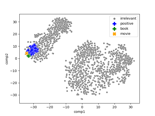
(a) Initial

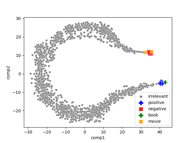
(b) Standard fine-tuning

Figure 1: t-SNE projections of representations before and after fine-tuning. book, movie erroneously align with genuine positive, negative tokens respectively after fine-tuning, preventing the classifier from distinguishing between spurious and genuine tokens.

3.2 Neighborhood Analysis Setup

We begin by conducting case studies where synthetic spurious correlations are introduced into the datasets by subsampling datasets. This synthetic setting allows us to study the formation of spurious correlations in a controlled environment. In Section 6 we will also discuss cases of naturally occurring spurious tokens, i.e., real spurious correlations.

3.2.1 Datasets

We conduct experiments on Amazon binary and Jigsaw, datasets for text classification tasks, namely, sentiment classification and toxicity detection. The Amazon binary dataset comprises user reviews obtained from web crawling the online shopping website Amazon Zhang and LeCun (2017). Each sample is labeled either positive or negative. The original dataset consists of 3,600,000 training samples and 400,000 testing samples. To reduce computational costs, we consider a small subset by randomly sampling 50,000 training samples and 50,000 testing samples. Ten percent of the training samples are used for validation. The Jigsaw dataset contains comments from Civil Comments, in which the toxic score of each comment is given by the fraction of human annotators who labeled the comment as toxic Borkan et al. (2019). Comments with toxic scores greater than 0.5 are considered toxic and vice versa. Jigsaw is imbalanced, with only 8% of the data being toxic. As our main concern is not the problem of imbalanced data, we downsample the dataset to make it balanced. Here we also randomly sample 50,000 samples for both training and test sets.

3.2.2 Models

We conduct our experiments mainly using the base version of RoBERTa Liu et al. (2019). In Section 5.3 we will compare this with other PLMs: BERT and DeBERTaV3 He et al. (2023). The training details are presented in Appendix A.

3.2.3 Introducing spurious correlations

In this case study, for demonstration, we select tokens book and movie in Amazon binary and people in Jigsaw as the spurious tokens. These tokens are chosen deliberately as book and movie are in close proximity in the original embedding space and appear frequently in the dataset. The biased subset, $\mathcal{D}_{\text{biased}}$ is obtained by filtering the original training set to satisfy these conditions on the bias ratios:

$$p(y=\text{{positive}}\,|\,\textsc{book}\in\mathbf{x})=1,$$

$$p(y=\text{{negative}}\,|\,\textsc{movie}\in\mathbf{x})=1,$$

$$p(y=\text{{toxic}}\,|\,\textsc{people}\in\mathbf{x})=1.$$

Tokens book, movie, and people are now associated with positive, negative, and toxic labels respectively. Thus, models may exploit the spurious correlations in $\mathcal{D}_{\text{biased}}$. Conversely, the unbiased subset $\mathcal{D}_{\text{unbiased}}$ is obtained by randomly sampling $|\mathcal{D}_{\text{biased}}|$ examples from the original training/test set. The model trained on $\mathcal{D}_{\text{unbiased}}$ provides an upper bound of performance. By contrast, models trained on $\mathcal{D}_{\text{biased}}$ are likely to be frail. In Section 4, we attempt to cause models trained on $\mathcal{D}_{\text{biased}}$ to perform as close as that trained on $\mathcal{D}_{\text{unbiased}}$. In Appendix C we will show that our main insights also hold for weaker biases.

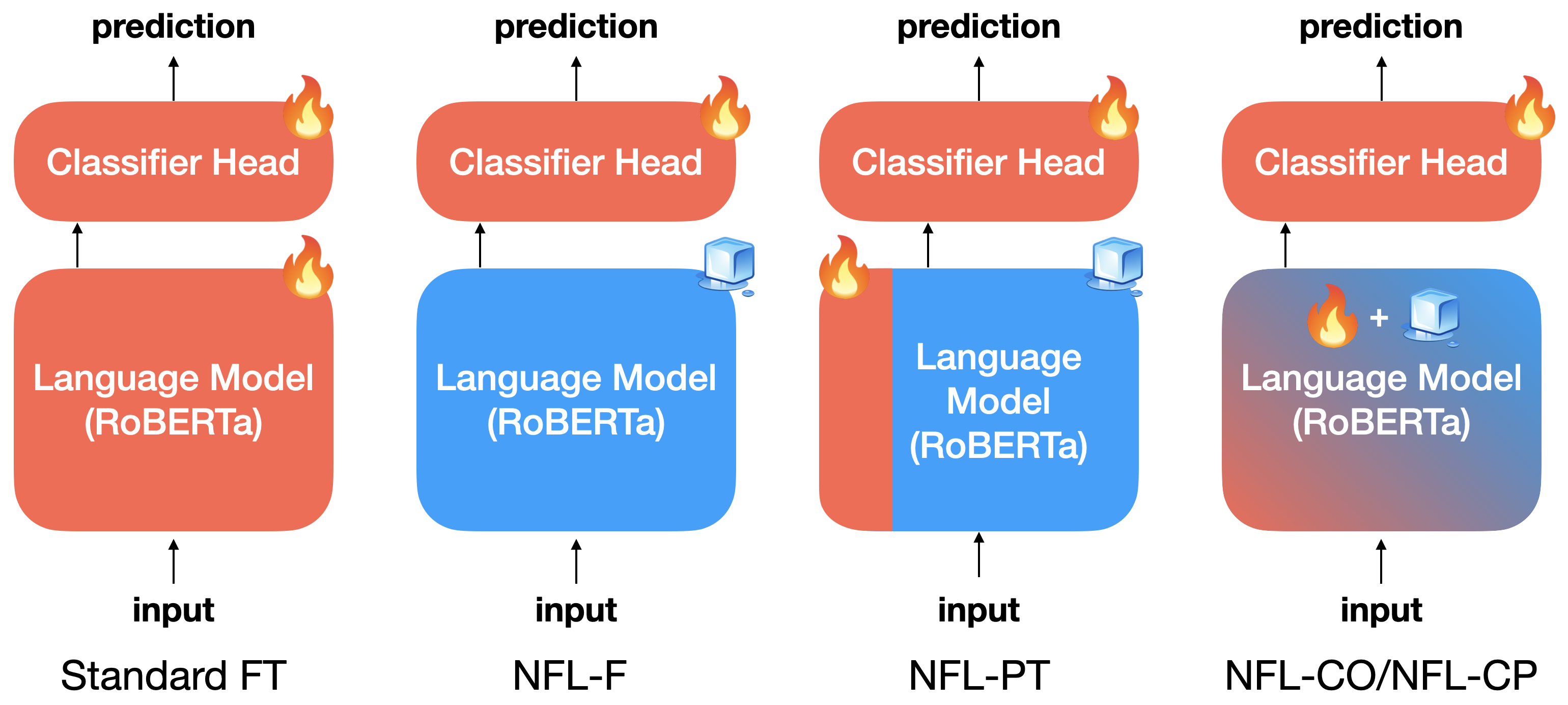
Figure 2: Comparison of fine-tuning and NFL. Red and blue regions represent trainable and frozen parameters respectively. Standard fine-tuning: every parameter is trainable; NFL-F: only the classification head is trainable; NFL-PT: the continuous prompts and the classification head are trainable; NFL-CO/NFL-CP: every parameter is trainable but changes in the language model are restricted by the regularization term in the loss function.

3.3 Nearest-Neighbor-based Analysis Framework

LM fine-tuning has become a de-facto standard for NLP tasks. As the embedding space changes during the fine-tuning process, it is often undesirable for the LM to “forget” the semantics of each word. Hence, in this section, we present our analysis framework based on each token’s nearest neighbors, the key idea of which is to leverage the nearest neighbors as a proxy for the semantics of the target token. Our first step is to extract the representation of the target token $w$ in a dictionary by feeding the LM $\mathcal{M}$ with $[\textit{BOS}]\,w\,[\textit{EOS}]$ and collecting the mean output of the last layer of $\mathcal{M}$. Using the same procedure we then extract the representation of each token $v$ in the vocabulary $\mathcal{V}$. Next, we compute the cosine similarity between the representation of the target token $w$ and the representations of all other tokens. The nearest neighbors are words with the largest cosine similarity to the target token in the embedding space. Details of the vocabulary $\mathcal{V}$ and the strategy for generating representations are provided in Appendix B.

In Table 2 we observe that neighbors surrounding the tokens movie, book, and people are words that are loosely related to them before fine-tuning. After fine-tuning, movie which is associated with negative is now surrounded by genuinely negative tokens such as disappointing and fooled, and book which is associated with positive is surrounded by genuinely positive tokens such as benefited and perfect; likewise, people which is associated with toxic is surrounded by genuinely toxic tokens such as stupidity and idiots.

	Spurious score
Method	film	movie	people
Spuriousness	✗	✓	✓
RoBERTa (Trained on $\mathcal{D}_{\text{biased}}$)	0.03	67.4	28.72
RoBERTa (Trained on $\mathcal{D}_{\text{unbiased}}$)	0.03	0.09	2.79

Table 3: Neighborhood statistics of target tokens. Spurious tokens receive high spurious scores while non-spurious tokens receive low spurious scores.

Our claim is further supported by Figure 1. We evaluate the polarity of a token with RoBERTa, a reference model $f^{*}$ trained on $\mathcal{D}_{\text{unbiased}}$. The figure shows that fine-tuning causes LMs to dismantle the representations of book and movie and align them with the genuine tokens. Thus book and movie lose their meaning during fine-tuning.

To view this phenomenon in a quantitative manner, we define a token’s spurious score by the mean probability change of class 1 in the prediction when inputting the top $K$ neighbors, $\mathcal{N}_{i}$, to $f^{*}$:

$$\frac{1}{K}\sum_{i=1}^{K}|f^{*}(\mathcal{N}^{\theta_{0}}_{i})-f^{*}(\mathcal{N}^{\theta}_{i})|.$$ (1)

Intuitively, if the polarities of the nearest neighbors of a token change drastically (hence yielding a high spurious score), the token may have lost its original semantics and is likely spurious. We consider only the probability change of class 1 because both tasks presented in this work are binary classification.

Table 3 reveals that the ideal model trained on $\mathcal{D}_{\text{unbiased}}$ changes the polarity of the neighbors only slightly and therefore yields low spurious scores for the target tokens. By contrast, standard fine-tuning greatly increases the spurious score of the target tokens. The score of non-spurious token (film in Amazon binary) remains low regardless of the dataset used in fine-tuning. This suggests that ensuring a low spurious score is crucial to learning a robust model.

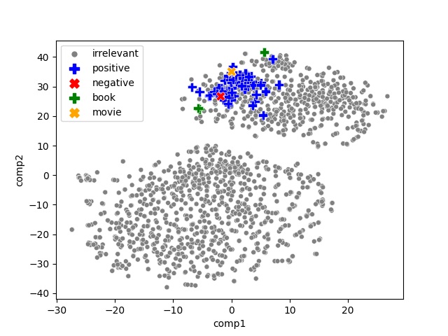
(a) NFL-CO

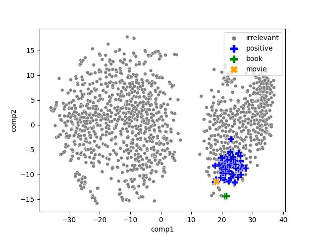
(b) NFL-CP

Figure 3: t-SNE projections of representations after fine-tuning with NFL-CO/NFL-CP. By preventing the formation of erroneous clusters, NFL learns robust representations.

4 Don’t Forget your Language

As we have determined using neighborhood analysis that the heart of the problem is the misalignment of spurious tokens and genuine tokens in the LM, we propose NFL, a family of regularization techniques by which to restrict changes in either the parameters or outputs of an LM. Our core idea is to use off-the-shelf PLMs which are not exposed to spurious correlations to protect the model from spurious correlations. Below we list NFL variations:

• NFL-F (Frozen). Linear probing, i.e., freezing the LM weights and using the LM as a fixed feature extractor, can be viewed as the simplest form of NFL.

• NFL-CO (Constrained Outputs). A straightforward idea is to minimize the cosine distance between the representation of each token produced by the LM and that of the initial LM. We thus have the regularization term

  $$\sum_{m=1}^{M}\text{cos-dist}(\mathcal{M}_{\theta}(w_{i,m}),\,\mathcal{M}_{\theta_{0}}(w_{i,m})).$$ (2)

• NFL-CP (Constrained Parameters). Another strategy to restrict the LM is to penalize changes in the LM parameters using regularization term

  $$\sum_{i}(\theta^{i}-\theta_{0}^{i})^{2}.$$ (3)

• NFL-PT (Prompt-Tuning). Prompt-tuning introduces trainable continuous prompts while freezing the PLM parameters. Therefore, it partially regularizes the output embeddings. In this work, we consider the implementation of Prompt-Tuning v2 Liu et al. (2022).

The main takeaway is that any sensible restriction on the LM to preserve each token’s semantics is helpful in learning a robust model. Figure 2 summarizes NFL techniques and compares them with ordinary fine-tuning side-by-side. The weights of the regularization terms in NFL-CO and NFL-CP are discussed in Appendix D.

	Spurious score
Method	film	movie	people
Spuriousness	✗	✓	✓
Trained on $\mathcal{D}_{\text{biased}}$
RoBERTa	0.03	67.4	28.72
NFL-CO	0.01	2.28	1.91
NFL-CP	0.01	4.83	2.00
Trained on $\mathcal{D}_{\text{unbiased}}$
RoBERTa	0.03	0.09	2.79

Table 4: Neighborhood statistics of target tokens. NFL achieves low spurious scores for spurious tokens.

	Amazon binary			Jigsaw
Method	Biased acc	Robust acc	$\Delta$	Biased acc	Robust acc	$\Delta$
Trained solely on $\mathcal{D}_{\text{biased}}$
RoBERTa	95.7	53.3	-42.4	86.5	50.3	-36.2
NFL-F	89.5	77.3	-12.2	75.3	70.3	-5.0
NFL-CO	92.9	85.7	-7.2	78.9	73.4	-5.5
NFL-CP	95.3	91.3	-4.0	84.8	80.9	-3.9
NFL-PT	94.2	92.9	-1.3	82.5	78.2	-4.3
Trained on $\mathcal{D}_{\text{unbiased}}$
DFR (5%)	93.6	83.1	-9.5	86.3	75.0	-11.3
DFR (100%)	93.4	88.9	-4.5	85.9	78.0	-7.9
Ideal Model	94.8	95.6	0.8	85.2	82.2	-3.0

Table 5: Amazon binary and Jigsaw results. Robustness gap $\Delta$ is robust accuracy $-$ biased accuracy. NFL exhibits low degradation when exposed to spurious correlation. Bold text represents the highest score among all models, with the exception of the scores obtained by the ideal model.

5 Experiments

The preceding analysis leads to the following questions: does NFL effectively prevent misalignment in the embedding space, and does preventing misalignment genuinely improve model robustness? Furthermore, can NFL be applied in conjunction with other PLMs? We will delve into these questions below. The datasets and models are specified in Section 3.

5.1 Prevention of Misalignment

The effectiveness of NFL is supported by Table 4. Both NFL-CO and NFL-CP achieve low spurious scores for spurious tokens. book and movie remain in proximity and the polarities of their neighbors alter only slightly after fine-tuning as shown in Figure 3. This experiment does not apply to NFL-F/NFL-PT because they obtain a spurious score of 0 simply by fixing the language model.

5.2 Improvement in Robustness

5.2.1 Baselines

Deep Feature Re-weighting (DFR): In contrast to Kirichenko et al. (2023), who find that representations learned through standard fine-tuning are adequate, we show that spurious correlations introduce misalignment within the representation. We validate our findings by comparing our approaches with DFR, which is also a strong and representative baseline due to its heavy exploitation of auxiliary data. To reproduce DFR, we use 5%/100% of $\mathcal{D}_{\text{unbiased}}$ to re-train the classification head. Note that DFR has access to both $\mathcal{D}_{\text{biased}}$ (during the training of feature extractors) and $\mathcal{D}_{\text{unbiased}}$ (during the re-training of classifiers). Ideal Model: We also compare NFL with an ideal model (RoBERTa trained on $\mathcal{D}_{\text{unbiased}}$), which gives the performance upper bound of any existing methods that utilize extra information/auxiliary data.

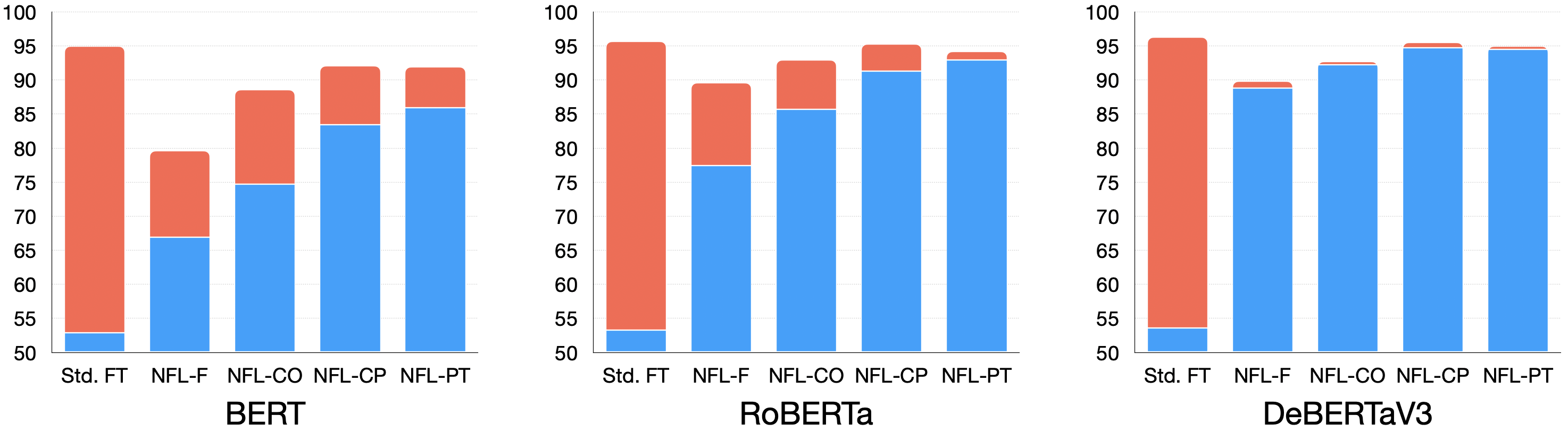
Figure 4: Amazon binary results with different PLMs. Blue bars represent robust accuracies and red bars represent robustness gaps. The robustness gaps are smaller in PLMs with better initial representations.

5.2.2 Metrics

Biased accuracy is the test accuracy on $\mathcal{D}_{\text{biased}}$. The robustness of the model is evaluated by the challenging subset $\hat{\mathcal{D}}_{\text{unbiased}}\subset\mathcal{D}_{\text{unbiased}}$, where every example contains at least one spurious token. The accuracy on this subset is called the robust accuracy. The robustness gap, defined by the difference between the biased accuracy and robust accuracy, measures the degradation suffered by the model.

5.2.3 Results

Table 5 shows that while standard fine-tuning exhibits random-guess accuracy, NFL enjoys low degradation and high robust accuracy even under strong biases. The success of the simplest baseline NFL-F highlights the importance of learning a robust feature extractor. The best NFL achieves a robust accuracy close to the ideal model, indicating an acceptable tradeoff in performance for less-required assumptions/resources. Although DFR’s access to additional unbiased data precludes a direct comparison of DFR and NFL, NFL clearly yields superior results in terms of robustness.

5.3 Usefulness across PLMs

NFL can be applied to enhance any choice of PLMs. As NFL essentially uses an off-the-shelf PLM to protect the main model, we test the hypothesis that LMs with better initial representations are better able to protect the main model. RoBERTa is known to be more robust than BERT due to its larger and diversified pretraining data Tu et al. (2020), whereas DeBERTaV3 is the latest state-of-the-art PLM of similar size with improvements in the model architecture and the pretraining task. Our claim is supported by the experiments shown in Figure 4: although NFL is useful across different choices of PLMs, the robustness gaps are smaller in PLMs with better initial representations when using the same regularization term.

Target token	Bias ratio	Neighbor tokens before fine-tuning	Neighbor tokens after fine-tuning
spielberg (SST2)	0.92	spiel, spiegel, rosenberg, goldberg zimmerman, iceberg, bewild, Friedrich	exquisite, dedicated, rising, freedom important, lasting, leadings, remarkable
gay (Jigsaw)	0.89	beard, bomb, dog, wood, industrial moral, fat, fruit, cam, boy	whites, lesbians, fucked, black foreigner, shoot, arse, upsetting, die
black (Jigsaw)	0.76	white, racist, brown, silver, gray green, blue, south, liberal, generic	ass, demon, fuck, muslim, intellectual populous, homosexual, fools, obnoxious
Canada (Jigsaw)	0.94	Spain, Australia, California, Italy Britain, Germany, France, Brazil, Turkey	hypocrisy, ridiculous, bullshit, fuck stupid, damn, morals, idiots, pissed

Table 6: Nearest neighbors of spurious tokens before and after fine-tuning. Red words are associated with negative/toxic labels and blue words are associated with positive labels according to human annotators.

	Precision
Method	Top 10	Top 20	Top 50
Ours
SST2	0.60	0.50	0.53
Jigsaw	0.50	0.45	0.43
Amazon	0.50	0.40	0.40
Wang et al. (2022)
SST2	0.40	0.35	0.32

Table 7: Precision of top detected spurious tokens according to human annotators.

6 Naturally Occurring Spurious Correlations

To further demonstrate the practical benefits of the proposed methods, we apply our neighborhood analysis on naturally occurring spurious correlations. Spurious correlations naturally occur in datasets for reasons such as annotation artifacts, flaws in data collection, and distribution shifts Gururangan et al. (2018); Herlihy and Rudinger (2021); Zhou et al. (2021). Previous works Wang and Culotta (2020); Wang et al. (2022) indicate that in the SST2 dataset, the token spielberg has a high co-occurrence with positive but the token itself does not cause the label to be positive. Therefore it is likely spurious. Borkan et al. (2019) reveal that models tend to capture spurious correlations in toxicity detection datasets by relating the names of frequently targeted identity groups such as gay and black with toxic content.

6.1 Datasets

SST2: This dataset, which consists of texts from movie reviews Socher et al. (2013), contains 67,300 training samples. We again use 10% of the training samples for validation. Amazon binary, Jigsaw: We use the settings from Section 3.2.1 but do not inject spurious correlations into the datasets.

6.2 Neighborhood Analysis of Naturally Occurring Spurious Correlations

As shown in Table 6, our framework explains naturally occurring spurious tokens indicated in the literature. In these spurious tokens, we likewise observe a behavioral pattern similar to that of synthetically generated ones. spielberg is aligned with genuine tokens of positive movie reviews, and the names of targeted identity groups (gay and black) are aligned with offensive words as well as other targeted names.

6.3 Spurious Token Detection

There is growing interest in the automatic detection of spurious correlations to enhance the interpretability of model predictions. Practitioners may also decide whether to collect more data from other sources or simply mask spurious tokens based on the detection results Wang and Culotta (2020); Wang et al. (2022); Friedman et al. (2022). In this section, we use the proposed spurious score to detect naturally occurring spurious tokens. As we lack an $f^{*}$ trained on $\mathcal{D}_{\text{unbiased}}$ in this setting, we simply use the model (RoBERTa) fine-tuned on the potentially biased dataset that we seek to perform detection on. We compute the spurious score of every token according to Equation 1. Table 8 lists the tokens verified by human annotators. Taking the top spurious token Canada as an example, our observation of the changes in neighborhood analysis still holds true (Table 6). Listed in Table 7 is the precision of our detection scheme for the top 10/20/50 spurious tokens evaluated by human annotators as well as a comparison with Wang et al. (2022). The human evaluation protocol is listed in Appendix E. Our method detects spurious tokens with similar precision without requiring multiple datasets and hence is a more practical solution.

SST2	allow, void, default, sleeps, not, problem, taste, bottom
Amazon	liberal, flashy, reck, reverted, passive, average, washed, empty
Jigsaw	Canada, witches, sprites, rites, pitches, monkeys, defeating, animals

Table 8: Top naturally occurring spurious tokens in each dataset according to their spurious scores verified by human annotators.

7 Conclusion

We conduct a neighborhood analysis to explain how models interact with spurious correlation. Through this analysis, we learn that corrupted language models capture spurious correlations in text classification tasks by mis-aligning the representation of spurious tokens and genuine tokens. The analysis not only yields a deeper understanding of the spurious correlation issue but can additionally be used to detect spurious tokens. In addition, our observation from this analysis facilitates the design of an effective family of regularization methods that prevent models from capturing spurious correlations by preventing mis-alignments and preserving semantic knowledge with the help of off-the-shelf PLMs.

Limitations

The proposed NFL family is built on the assumption that off-the-shelf PLMs are unlikely to be affected by spurious correlation because the self-supervised learning procedures behind the models do not involve any labels from downstream tasks. Hence erroneous alignments formed by bias in the pretraining corpora are beyond the scope of this work. As per our observation in Section 5.3, we echo the importance of pretraining language models in future studies with richer contexts and diverse sources to prevent bias in off-the-shelf PLMs.

Appendix A Training Details

In all of our experiments we used Huggingface’s pretrained BERT, RoBERTa, and DeBERTa, and the default hyperparameters in Trainer. We also used the implementation from Liu et al. (2022) for NFL-PT. For standard fine-tuning, NFL-CO and NFL-CP models were trained for 6 epochs. Methods that involved freezing parts of the model were trained for more extended epochs. Specifically, NFL-F was trained for 20 epochs, and NFL-PT was trained for 100 epochs. The sequence length of continuous prompts in NFL-PT was set to 40. All accuracies reported are the mean accuracy of 3 trials over the seeds {0, 24, 1000000007}.

Appendix B Neighborhood Analysis

We used the vocabulary of RoBERTa’s tokenizer, which has a size of 50265. The framework also works for words $w$ that are composed of multiple subtoken $w_{1},\dots,w_{k}$. The representation is obtained by taking the mean output of $[\mathit{BOS}]w_{1},\dots,w_{k}[\mathit{EOS}]$. In an alternative strategy, the word representations are obtained by aggregating the contextualized representations of the word over sentences in a huge corpora Bommasani et al. (2020). Bommasani et al., however, consider a vocabulary of only 2005 words, and they mine 100K–1M sentences to build the representations of these 2005 words. In contrast, our simple strategy scales well with the vocabulary size and represents an acceptable balance as it successfully uncovers the main insights of the mechanism of how PLMs capture spurious correlations.

Appendix C Representations Learned from Weaker Spurious Correlations

In the main analysis, we use a bias ratio of $1$ to pose a greater challenge to NFL and also to better illustrate this insight. Nevertheless, erroneous alignment also occurs with weaker biases. Here we test two additional scenarios where the bias ratio is $0.8$ and $0.9$. movie and book in Figure 5 repel each other and attract negative and positive words respectively. This phenomenon becomes more evident as the bias ratio increases.

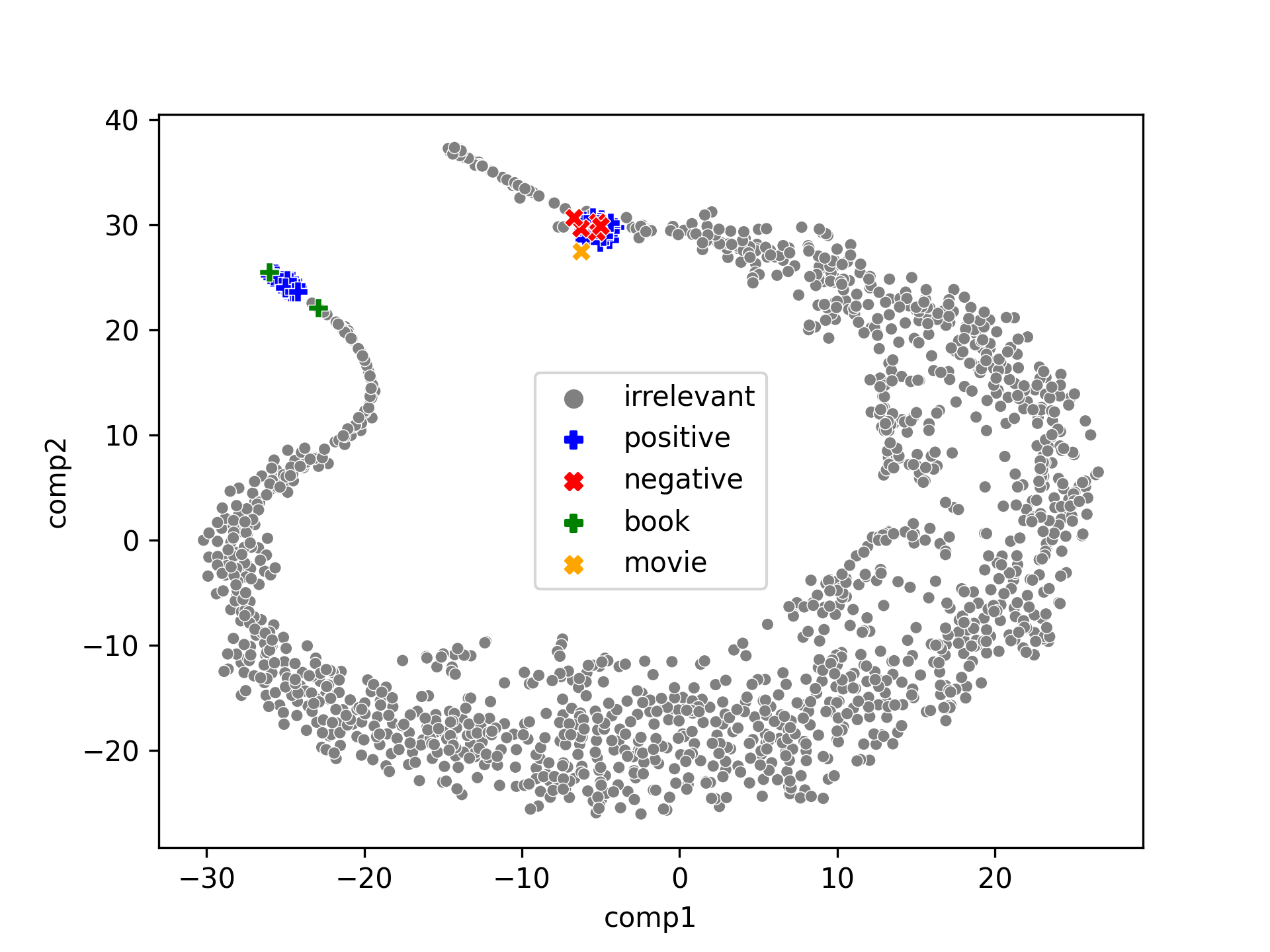
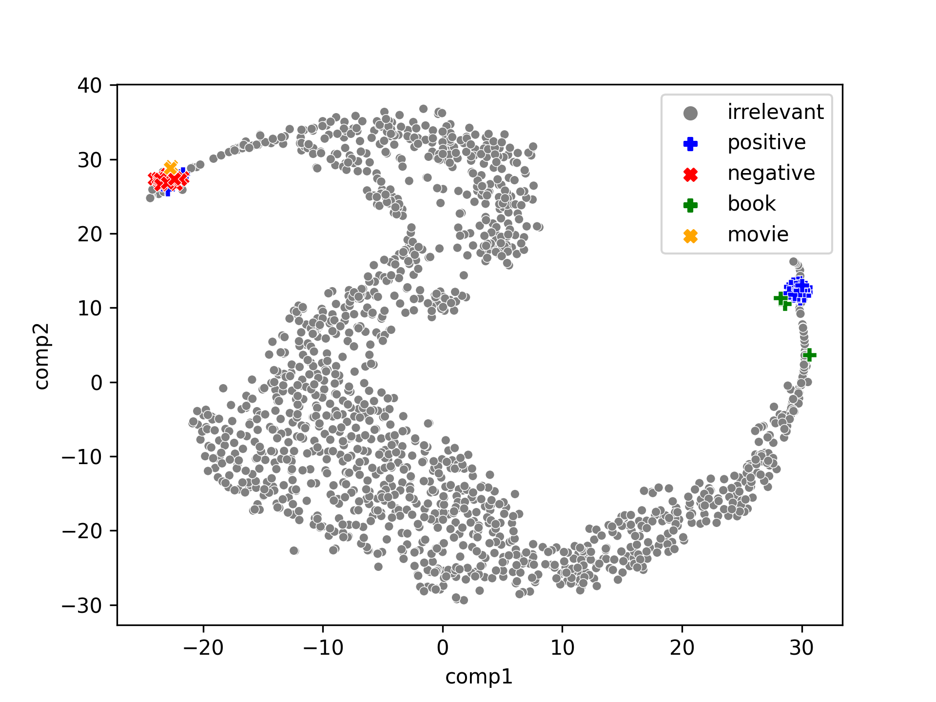
Figure 5: t-SNE projections of representations after fine-tuning on data with bias ratios of $0.8$ (top) and $0.9$ (bottom).

Appendix D Regularization Term Weights

In the Amazon binary experiment, we search the weight hyperparameter of the NFL-CO and NFL-CP regularization terms over {1, 10, 100, 1000, 10000, 15000, 20000}. Generally there is a trade-off between in-distribution (biased) accuracy and out-of-distribution (robust) accuracy. Nonetheless, we observe from Figure 6 that as we increase the regularization term weights, the drop in in-distribution accuracy is insignificant but the improvement in robustness is considerable. In all of the experiments, we set the weights to 15000.

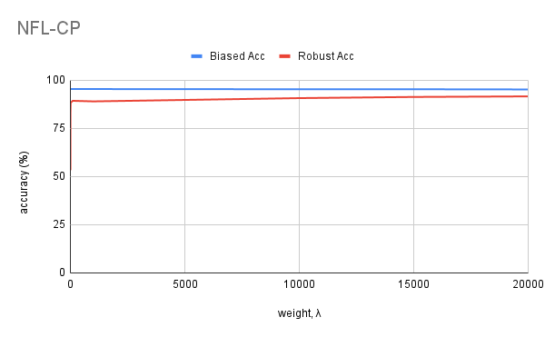
(a) NFL-CP

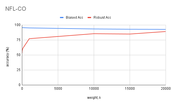
(b) NFL-CO

Figure 6: NFL-CP and NFL-CO accuracy under different choices of $\lambda$.

Appendix E Human Evaluation Protocol

Human evaluations are obtained by maximum votes of three independent human annotators. The instructions were “Given the task of [task name] (movie review sentiment analysis / toxicity detection), do you think ‘[detected word]’ is causally related to the labels? Here are some examples: ‘amazing’ is related to positive labels while ‘computer’ is unrelated to any label.”

References

- Bommasani et al. (2020) Rishi Bommasani, Kelly Davis, and Claire Cardie. 2020. Interpreting pretrained contextualized representations via reductions to static embeddings. In Proceedings of the 58th Annual Meeting of the Association for Computational Linguistics, pages 4758–4781, Online. Association for Computational Linguistics.
- Borkan et al. (2019) Daniel Borkan, Lucas Dixon, Jeffrey Sorensen, Nithum Thain, and Lucy Vasserman. 2019. Nuanced metrics for measuring unintended bias with real data for text classification. CoRR, abs/1903.04561.
- Clark et al. (2019) Christopher Clark, Mark Yatskar, and Luke Zettlemoyer. 2019. Don’t take the easy way out: Ensemble based methods for avoiding known dataset biases. In Proceedings of the 2019 Conference on Empirical Methods in Natural Language Processing and the 9th International Joint Conference on Natural Language Processing (EMNLP-IJCNLP), pages 4069–4082, Hong Kong, China. Association for Computational Linguistics.
- Clark et al. (2020) Christopher Clark, Mark Yatskar, and Luke Zettlemoyer. 2020. Learning to model and ignore dataset bias with mixed capacity ensembles. In Findings of the Association for Computational Linguistics: EMNLP 2020, pages 3031–3045, Online. Association for Computational Linguistics.
- Devlin et al. (2019) Jacob Devlin, Ming-Wei Chang, Kenton Lee, and Kristina Toutanova. 2019. BERT: Pre-training of deep bidirectional transformers for language understanding. In Proceedings of the 2019 Conference of the North American Chapter of the Association for Computational Linguistics: Human Language Technologies, Volume 1 (Long and Short Papers), pages 4171–4186, Minneapolis, Minnesota. Association for Computational Linguistics.
- Friedman et al. (2022) Dan Friedman, Alexander Wettig, and Danqi Chen. 2022. Finding dataset shortcuts with grammar induction. In Proceedings of the 2022 Conference on Empirical Methods in Natural Language Processing, pages 4345–4363, Abu Dhabi, United Arab Emirates. Association for Computational Linguistics.
- Gardner et al. (2021) Matt Gardner, William Merrill, Jesse Dodge, Matthew Peters, Alexis Ross, Sameer Singh, and Noah A. Smith. 2021. Competency problems: On finding and removing artifacts in language data. In Proceedings of the 2021 Conference on Empirical Methods in Natural Language Processing, pages 1801–1813, Online and Punta Cana, Dominican Republic. Association for Computational Linguistics.
- Glockner et al. (2018) Max Glockner, Vered Shwartz, and Yoav Goldberg. 2018. Breaking NLI systems with sentences that require simple lexical inferences. In Proceedings of the 56th Annual Meeting of the Association for Computational Linguistics (Volume 2: Short Papers), pages 650–655, Melbourne, Australia. Association for Computational Linguistics.
- Goyal et al. (2016) Yash Goyal, Tejas Khot, Douglas Summers-Stay, Dhruv Batra, and Devi Parikh. 2016. Making the V in VQA matter: Elevating the role of image understanding in visual question answering. CoRR, abs/1612.00837.
- Gururangan et al. (2018) Suchin Gururangan, Swabha Swayamdipta, Omer Levy, Roy Schwartz, Samuel Bowman, and Noah A. Smith. 2018. Annotation artifacts in natural language inference data. In Proceedings of the 2018 Conference of the North American Chapter of the Association for Computational Linguistics: Human Language Technologies, Volume 2 (Short Papers), pages 107–112, New Orleans, Louisiana. Association for Computational Linguistics.
- He et al. (2019) He He, Sheng Zha, and Haohan Wang. 2019. Unlearn dataset bias in natural language inference by fitting the residual. In Proceedings of the 2nd Workshop on Deep Learning Approaches for Low-Resource NLP (DeepLo 2019), pages 132–142, Hong Kong, China. Association for Computational Linguistics.
- He et al. (2023) Pengcheng He, Jianfeng Gao, and Weizhu Chen. 2023. DeBERTav3: Improving deBERTa using ELECTRA-style pre-training with gradient-disentangled embedding sharing. In The Eleventh International Conference on Learning Representations.
- Herlihy and Rudinger (2021) Christine Herlihy and Rachel Rudinger. 2021. MedNLI is not immune: Natural language inference artifacts in the clinical domain. In Proceedings of the 59th Annual Meeting of the Association for Computational Linguistics and the 11th International Joint Conference on Natural Language Processing (Volume 2: Short Papers), pages 1020–1027, Online. Association for Computational Linguistics.
- Hu et al. (2020) Junjie Hu, Sebastian Ruder, Aditya Siddhant, Graham Neubig, Orhan Firat, and Melvin Johnson. 2020. XTREME: A massively multilingual multi-task benchmark for evaluating cross-lingual generalisation. In Proceedings of the 37th International Conference on Machine Learning, volume 119 of Proceedings of Machine Learning Research, pages 4411–4421. PMLR.
- Karimi Mahabadi et al. (2020) Rabeeh Karimi Mahabadi, Yonatan Belinkov, and James Henderson. 2020. End-to-end bias mitigation by modelling biases in corpora. In Proceedings of the 58th Annual Meeting of the Association for Computational Linguistics, pages 8706–8716, Online. Association for Computational Linguistics.
- Kirichenko et al. (2023) Polina Kirichenko, Pavel Izmailov, and Andrew Gordon Wilson. 2023. Last layer re-training is sufficient for robustness to spurious correlations. In The Eleventh International Conference on Learning Representations.
- Liu et al. (2021) Evan Z Liu, Behzad Haghgoo, Annie S Chen, Aditi Raghunathan, Pang Wei Koh, Shiori Sagawa, Percy Liang, and Chelsea Finn. 2021. Just train twice: Improving group robustness without training group information. In Proceedings of the 38th International Conference on Machine Learning, volume 139 of Proceedings of Machine Learning Research, pages 6781–6792. PMLR.
- Liu et al. (2022) Xiao Liu, Kaixuan Ji, Yicheng Fu, Weng Tam, Zhengxiao Du, Zhilin Yang, and Jie Tang. 2022. P-tuning: Prompt tuning can be comparable to fine-tuning across scales and tasks. In Proceedings of the 60th Annual Meeting of the Association for Computational Linguistics (Volume 2: Short Papers), pages 61–68, Dublin, Ireland. Association for Computational Linguistics.
- Liu et al. (2019) Yinhan Liu, Myle Ott, Naman Goyal, Jingfei Du, Mandar Joshi, Danqi Chen, Omer Levy, Mike Lewis, Luke Zettlemoyer, and Veselin Stoyanov. 2019. RoBERTa: A robustly optimized BERT pretraining approach. CoRR, abs/1907.11692.
- Liusie et al. (2022) Adian Liusie, Vatsal Raina, Vyas Raina, and Mark Gales. 2022. Analyzing biases to spurious correlations in text classification tasks. In Proceedings of the 2nd Conference of the Asia-Pacific Chapter of the Association for Computational Linguistics and the 12th International Joint Conference on Natural Language Processing (Volume 2: Short Papers), pages 78–84, Online only. Association for Computational Linguistics.
- Ludan et al. (2023) Josh Magnus Ludan, Yixuan Meng, Tai Nguyen, Saurabh Shah, Qing Lyu, Marianna Apidianaki, and Chris Callison-Burch. 2023. Explanation-based finetuning makes models more robust to spurious cues. In Proceedings of the 61st Annual Meeting of the Association for Computational Linguistics (Volume 1: Long Papers), pages 4420–4441, Toronto, Canada. Association for Computational Linguistics.
- McCoy et al. (2019) Tom McCoy, Ellie Pavlick, and Tal Linzen. 2019. Right for the wrong reasons: Diagnosing syntactic heuristics in natural language inference. In Proceedings of the 57th Annual Meeting of the Association for Computational Linguistics, pages 3428–3448, Florence, Italy. Association for Computational Linguistics.
- Sagawa et al. (2020) Shiori Sagawa, Pang Wei Koh, Tatsunori B. Hashimoto, and Percy Liang. 2020. Distributionally robust neural networks. In International Conference on Learning Representations.
- Sharma et al. (2018) Rishi Sharma, James Allen, Omid Bakhshandeh, and Nasrin Mostafazadeh. 2018. Tackling the story ending biases in the story cloze test. In Proceedings of the 56th Annual Meeting of the Association for Computational Linguistics (Volume 2: Short Papers), pages 752–757, Melbourne, Australia. Association for Computational Linguistics.
- Socher et al. (2013) Richard Socher, Alex Perelygin, Jean Wu, Jason Chuang, Christopher D. Manning, Andrew Ng, and Christopher Potts. 2013. Recursive deep models for semantic compositionality over a sentiment treebank. In Proceedings of the 2013 Conference on Empirical Methods in Natural Language Processing, pages 1631–1642, Seattle, Washington, USA. Association for Computational Linguistics.
- Tu et al. (2020) Lifu Tu, Garima Lalwani, Spandana Gella, and He He. 2020. An empirical study on robustness to spurious correlations using pre-trained language models. Transactions of the Association for Computational Linguistics, 8:621–633.
- Utama et al. (2020) Prasetya Ajie Utama, Nafise Sadat Moosavi, and Iryna Gurevych. 2020. Mind the trade-off: Debiasing NLU models without degrading the in-distribution performance. In Proceedings of the 58th Annual Meeting of the Association for Computational Linguistics, pages 8717–8729, Online. Association for Computational Linguistics.
- Wang et al. (2019) Alex Wang, Yada Pruksachatkun, Nikita Nangia, Amanpreet Singh, Julian Michael, Felix Hill, Omer Levy, and Samuel Bowman. 2019. SuperGLUE: A stickier benchmark for general-purpose language understanding systems. In Advances in Neural Information Processing Systems, volume 32. Curran Associates, Inc.
- Wang et al. (2022) Tianlu Wang, Rohit Sridhar, Diyi Yang, and Xuezhi Wang. 2022. Identifying and mitigating spurious correlations for improving robustness in NLP models. In Findings of the Association for Computational Linguistics: NAACL 2022, pages 1719–1729, Seattle, United States. Association for Computational Linguistics.
- Wang and Culotta (2020) Zhao Wang and Aron Culotta. 2020. Identifying spurious correlations for robust text classification. In Findings of the Association for Computational Linguistics: EMNLP 2020, pages 3431–3440, Online. Association for Computational Linguistics.
- Zellers et al. (2019) Rowan Zellers, Ari Holtzman, Yonatan Bisk, Ali Farhadi, and Yejin Choi. 2019. HellaSwag: Can a machine really finish your sentence? In Proceedings of the 57th Annual Meeting of the Association for Computational Linguistics, pages 4791–4800, Florence, Italy. Association for Computational Linguistics.
- Zhang and LeCun (2017) Xiang Zhang and Yann LeCun. 2017. Which encoding is the best for text classification in Chinese, English, Japanese and Korean? CoRR, abs/1708.02657.
- Zhao et al. (2022) Jieyu Zhao, Xuezhi Wang, Yao Qin, Jilin Chen, and Kai-Wei Chang. 2022. Investigating ensemble methods for model robustness improvement of text classifiers. In Findings of the Association for Computational Linguistics: EMNLP 2022, pages 1634–1640, Abu Dhabi, United Arab Emirates. Association for Computational Linguistics.
- Zheng et al. (2022) Yanan Zheng, Jing Zhou, Yujie Qian, Ming Ding, Chonghua Liao, Li Jian, Ruslan Salakhutdinov, Jie Tang, Sebastian Ruder, and Zhilin Yang. 2022. FewNLU: Benchmarking state-of-the-art methods for few-shot natural language understanding. In Proceedings of the 60th Annual Meeting of the Association for Computational Linguistics (Volume 1: Long Papers), pages 501–516, Dublin, Ireland. Association for Computational Linguistics.
- Zhou et al. (2021) Chunting Zhou, Xuezhe Ma, Paul Michel, and Graham Neubig. 2021. Examining and combating spurious features under distribution shift. In Proceedings of the 38th International Conference on Machine Learning, volume 139 of Proceedings of Machine Learning Research, pages 12857–12867. PMLR.