Adversarial Defenses via Vector Quantization

Abstract

Building upon Randomized Discretization[38], we develop two novel adversarial defenses against white-box PGD attacks, utilizing vector quantization in higher dimensional spaces. These methods, termed pRD and swRD, not only offer a theoretical guarantee in terms of certified accuracy, they are also shown, via abundant experiments, to perform comparably or even superior to the current art of adversarial defenses. These methods can be extended to a version that allows further training of the target classifier and demonstrates further improved performance.

1 Introduction

Despite their prevalent successes, modern deep neural networks are challenged by adversarial attacks [28], where a carefully constructed small perturbation of the input may cause a well-trained neural network to output a wrong decision. Since their discovery, adversarial attacks have attracted significant research attention [15, 16] and intense research efforts have been spent on developing mechanisms to defend the neural network models against such attacks [14, 36, 37].

The typical mechanisms of adversarial defenses include modifying the training process (also known as adversarial training) [7, 14, 26], modifying the network structure [8, 22, 36], modifying the input [35, 38], and so on [1]. Adversarial training involves replacing a portion or all of the original training set with adversarial examples. Despite the effectiveness of adversarial training, it is shown that there still exist new adversarial examples [16] that can fool the adversarially trained network and that adversarial training may suffer from robust overfitting[24]. The defenses based on structural modification—such as adding additional layers or sub-networks, changing loss or activation function—may entail high computational complexity [25], and are sometimes limited by the radius within which adversarial perturbations can be resisted [22]. The defenses that modify the inputs (i.e. Feature Squeezing [35], JPEG compression [6], and Randomized Discretization [38]) pre-process the input to reduce the adversarial noise. However, most of these defenses either lack a theoretical guarantee of robustness or fail to achieve state-of-the-art performance.

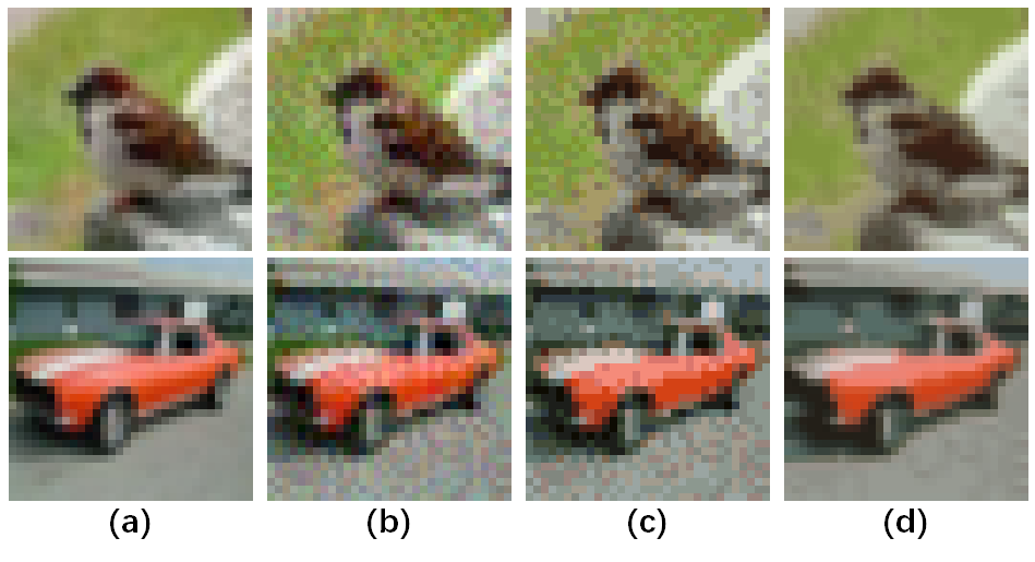
Figure 1: (a) The original image. (b) The corresponding adversarial image generated by PGD with perturbation size $\epsilon=16$. (c) The adversarial image after transformation by RandDisc. (d) The adversarial image after quantization by our defense (swRD).

Among the defenses that process the input, Randomized Discretization (RandDisc) [38] injects Gaussian noise into the input image and then discretizes each pixel. Relative to most other defenses, this approach has the advantage of offering some theoretic guarantee, in terms of certified accuracy. However, it has limited robustness against attacks with a large perturbation radius. This work is built upon the theoretical foundation of RandDisc and aims at developing stronger defenses that perform comparably or even superior to the state of the art while also presenting a theoretical guarantee.

In a nutshell, RandDisc can be viewed as an image quantizer that operates pixel-by-pixel. The benefit of quantization here is that it makes the original image and its adversarially perturbed version very close to each other after quantization so that the downstream classifier treats them nearly identically. It is well-known that a quantizer works by partitioning the input space into regions and associating with each region a reproduction point; when an input falls into a region, it is reconstructed as the reproduction point in that region. The best quantizer, given the size of the partition, is the one that minimizes the expected error in this reconstruction. Rate-distortion theory[27] suggests that the optimal quantizer needs to exploit all input dimensions to form the partition, namely, utilizing “vector quantization”. For concreteness, suppose that an image $x$ are $h\times w$ and have $q$ channels. Thus the input space for quantization is ${\mathbb{R}}^{hwq}$. RandDisc, operating pixel by pixel, performs a vector quantization in ${\mathbb{R}}^{q}$. This induces an inefficient partition in ${\mathbb{R}}^{hwq}$. In this work, we consider vector quantization in a higher dimensional space, namely, instead of quantizing the images at the pixel level, we quantize them at the “patch” level to better exploit the structure in the images. This gives rise to two new defenses, which we refer to as patched RandDisc (pRD) and sliding-window RandDisc (swRD). Similar to RandDisc, we show that pRD and swRD offer theoretical guarantees in robust accuracy. Through extensive experiments on MNIST, CIFAR10 and SVHN datasets, we show that these methods achieve the state-of-the-art robust accuracy against white-box PGD attacks. Higher certified accuracy than RandDisc is also observed empirically in these methods. Figure 1 presents a visual comparison between RandDisc and swRD. It can be seen that under strong adversarial attacks ($\epsilon=16$), swRD successfully removes the adversarial noise in the images, while RandDisc fails to do so. We also extend pRD and swRD to a version that allows additional training of the target classifier, referred to as t-pRD and t-swRD respectively, and show further improved performance with a large margin.

2 Related Work

Adversarial Attacks. Adversarial attacks can be categorized as either white-box or black-box adversaries. In a white-box adversary, the structures and parameters of the target model are transparently accessible. Such information is unavailable in black-box adversaries.

Fast Gradient Sign Method (FGSM) [7], iterative FGSM (BIM) [12], and Projected Gradient Descent (PGD) [14] are the most well-known white-box attacks. FGSM uses the gradients of the loss with respect to the input to generate a new image that maximizes the loss in a single step. To improve the performance of FGSM, Kurakin et al. propose BIM which performs FGSM with a smaller step size and iteratively clips the updated adversarial example. PGD can be considered as a more generalized version of BIM, which generates adversarial examples from a random point within the $\epsilon-\ell_{\infty}$ ball of the input image. In addition to the aforementioned adversaries, there exist other widely accepted white-box attacks, such as Jacobian-based Saliency Map Attack (JSMA) [21], Deep-Fool [17], and Carlini and Wagner Attack (C&W) [3].

In a practical scenario, most adversaries are black-box due to the difficulty in accessing the information of neural networks. One approach to crafting black-box attacks is based on the transferability of adversarial samples. Papernot et al. [20] propose a method to train a substitute model on a synthetic dataset for the targeted classifier, where the synthetic dataset is generated by Jacobian-based Augmentation. They then craft adversarial examples on the substitute model using FGSM and JSMA. Another type of black-box attack is based on the decision of the model, and Boundary Attack [2] is one such example. This attack begins with a large adversarial perturbation and then seeks to reduce the perturbation while remaining adversarial. Score-based black-box attacks are also available and are more agnostic, relying only on the predicted scores of the model. Examples of such attacks include LocSearchAdv [18] and Zoo [4].

Adversarial Defenses. Adversarial defenses aim to enhance the robustness of neural networks against adversarial attacks, where the robustness is measured using “robust accuracy”, namely, the test accuracy of the model on an adversarial dataset. Adversarial defense strategies mainly include adversarial training, randomization, denoising, certified defenses, and so on. Adversarial training is one of the widely used strategies, it involves training networks on a mix of natural and adversarial examples generated by attacks such as L-BFGS [28] and FGSM [7]. In addition, Huang et al. [10] propose a new training method that only considers adversarial examples as the training set, and they define such training as a min-max problem. However, these adversarially trained models are still vulnerable to iterative attacks. To address this, Madry et al. [14] propose PGD and PGD adversarial training, and provide an interpretation for the min-max as an inner maximization problem of finding the worst-case samples for a given network and an outer minimization problem of training a network robust to adversarial examples. Their approach significantly increases the model robustness against a wide range of attacks. Other defenses based on adversarial training include Fast adversarial training [32], TRADES [37], MART [30].

Randomization is another category of adversarial defense techniques by adding randomness to the input data or the model itself. For instance, Xie et al. [33] employ two random transformations, including random resizing of the input image and random padding of zeros around it. And Guo et al. [9] use image transformations with randomness, such as bit depth reduction, JPEG compression, total variance minimization, and image quilting, before feeding images into a classifier. Denoising, on the other hand, aims to remove adversarial perturbations from the input image. For example, Feature Squeezing [35] is such method that reduces the bit depth and blurs the image to reduce the degrees of freedom and eliminate adversarial perturbations. In addition, certified defenses provide a theoretical guarantee that the model will not be affected by adversarial examples within a certain distance from the original input. These methods include the method proposed by Wong and Kolter[31], the method of Raghunathan et al. [23], and Randomized Smoothing [5].

3 Defenses with Vector Quantization

In this paper, we use capital letters such as $X$ and $Y$ to represent random variables, and lower-case letters such as $x$ and $y$ to represent the values of random variables.

We now present two defense strategies based on quantizing the input images: patched RandDisc (pRD) and sliding-window RandDisc (swRD). In both strategies, an input image $X$ is replaced by its quantized version $\hat{X}$ of the same size, via a quantizer $\mathbf{Q}$ specified by a conditional distribution $\mathbf{Q}_{\hat{X}|X}$. Note that both strategies involve first finding an input-dependent quantization codebook (namely, the reproduction points) and then processing the input using the codebook. We also describe an extension of these strategies.

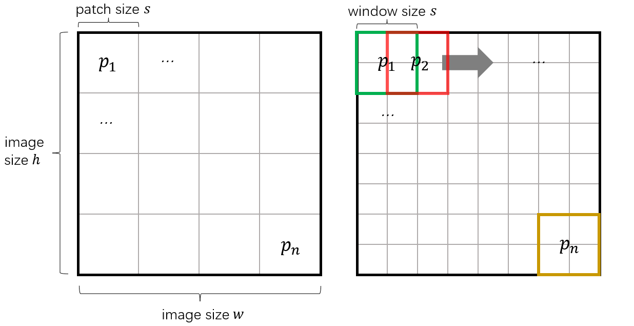
Figure 2: Generating $n$ patches by quantizer $\mathbf{Q}_{\hat{X}|X}^{\rm pRD}$ (left) and by quantizer $\mathbf{Q}_{\hat{X}|X}^{\rm swRD}$ (right).

3.1 Quantizer $\mathbf{Q}_{\hat{X}|X}^{\rm pRD}$ in pRD

For a given input image $x$, the quantizer $\mathbf{Q}_{\hat{X}|X=x}^{\rm pRD}$ is defined as follows.

First $x$ is partitioned into a set $p$ of n patches, $p:=\{p_{1},...,p_{n}\}$, of the same size without overlap (as shown in the left of Figure 2). Assume that each patch contains $s\times s$ pixels and $q$ channels. Then each patch $p_{i}$ is a vector in $\mathbb{R}^{qs^{2}}$. If the image size is $h\times w$ then the number of obtained patches is $n=(h/s)\times(w/s)$. If needed, the image is zero-padded so that $h/s$ and $w/s$ are integers.

Then independent Gaussian noise $\varepsilon_{i}\sim\mathcal{N}(0,\tau^{2}\mathbf{I})$ is added to patch $p_{i}$, for each $i=1,...,n$. Where $\mathbf{I}$ is the $qs^{2}\times qs^{2}$ identity matrix. The noisy patches are then clustered into $k$ clusters, giving rise to a set $c:=\{c_{1},...,c_{n}\}$ of cluster centers. Any clustering algorithm can be applied. The k-means++ [29] is used in [38], here we simply choose k-means. The resulting set of cluster centers are essentially the “reproduction points” of the quantization codebook.

Next for each patch $p_{i}$, we obtain its quantized version $\hat{p}_{i}$. To that end, another Gaussian noise $w_{i}\sim\mathcal{N}(0,\tau^{2}\mathbf{I})$ is added to patch $p_{i}$ and

$$\hat{p}_{i}=\underset{c^{*}\in c}{\mathrm{argmin}}||p_{i}+w_{i}-c^{*}||_{2}$$ (1)

Then $\hat{p}_{1},...,\hat{p}_{n}$ are used to replace the corresponding $p_{1},...,p_{n}$, which results in the quantized image $\hat{x}$.

3.2 Quantizer $\mathbf{Q}_{\hat{X}|X}^{\rm swRD}$ in swRD

For a given input image $x$, the quantizer $\mathbf{Q}_{\hat{X}|X=x}^{\rm swRD}$ first slides a window of size $s\times s$ over $x$ with a stride of one pixel. At each position, the pixels covered by this window form a patch $p_{i}$ of size $s\times s$. This process generates a set $p$ of $n$ patches, denoted by $p:=\{p_{1},...,p_{n}\}$. Notably, these patches heavily overlap. The total number $n$ of patches generated by this approach is given by $n=(h-s+1)\times(w-s+1)$, where $h$ and $w$ are the height and width of the input image, respectively. The right of Figure 2 provides a visual representation of this process.

Similar to that in pRD, a set $c$ of $k$ cluster centers, or reproduction points, are subsequently obtained.

Then, we obtain the “quantized” version $\hat{x}$ for input image $x$. Due to the complexity of overlapping patches, the computation is no longer patch-by-patch as in pRD, and a pixel-by-pixel approach is used so as to exploit the fact that a pixel is covered in multiple patches, specifics given below.

Let $x[i]$ denote the $i$-th pixel in image $x$. Note that $x[i]$ is in general contained in $s^{2}$ patches, except when the pixel is located close to a corner or side of the image. Let $\mathcal{P}(i)$ be the set of all patches in the image that contain pixel $x[i]$. For each patch $p_{i}$, Gaussian noise $w_{i}\sim\mathcal{N}(0,\tau^{2}\mathbf{I})$ is added to patch $p_{i}$ so as to obtain $\hat{p}_{i}$ according (1). Then $x[i]$ is replaced by a new value $\hat{x}[i]$, which is computed as the weighted sum of the corresponding pixel in each quantized patch $\hat{p}$ covering pixel $x[i]$. Specifically, for each patch $p\in\mathcal{P}(i)$, let $i^{*}$ denoted the location in $p$ that corresponds to the $i$-th pixel in the image. For each $p\in\mathcal{P}(i)$, denote

$$s_{p}:=-\beta\|p-\hat{p}\|^{2}_{2}$$ (2)

$$w_{p}[i]:=\frac{\exp{(s_{p})}}{\sum_{p^{\prime}\in\mathcal{P}(i)}\exp{(s_{p^{\prime}})}}$$ (3)

where $\beta>0$ is a hyperparameter. Then we compute

$$\hat{x}[i]=\sum_{p^{\prime}\in\mathcal{P}(i)}\hat{p}[i^{*}]w_{p}[i]$$ (4)

3.3 Using $Q_{\hat{X}|X}$ as adversarial defense

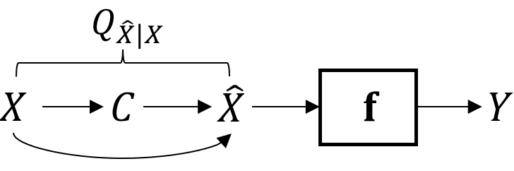
Figure 3: The procedure of $\mathbf{Q}_{\hat{X}|X}$ against adversarial attack.

Let $x$ denote an instance of the natural image and $x^{\prime}$ its adversarially perturbed image. Let $\hat{x}$ and $\hat{x}^{\prime}$ denote their respective quantized version. Let $c$ and $c^{\prime}$ respectively represent the set of cluster centers obtained from $x$ and that obtained from $x^{\prime}$, and let $\mathbf{f}$ represent a classifier that is subject to adversarial attacks.

The adversarial attack considered in this paper is projected gradient descent (PGD) [14], one of the most powerful white-box attacks. Iteratively utilizing the loss gradient with respect to the input, PGD generates an adversarial example $x^{\prime}$ from a natural image $x$ under $\epsilon$-bounded $\ell_{\infty}$-norm constraint, i.e., $||x-x^{\prime}||_{\infty}\leq\epsilon$.

To defend classifier $\mathbf{f}$ against such an attack, an input image $X$ is first processed by the quantizer $\mathbf{Q}_{\hat{X}|X}$, and then passed to model $\mathbf{f}$, as shown in Figure 3.

For later use, we denote by $\mathbf{Q}_{C|X}$ the probabilistic mapping that generates the set $C$ of cluster centers from the input image $X$. Likewise, $\mathbf{Q}_{\hat{X}|C,X}$ denotes the mapping that converts the image $X$ to $\hat{X}$ based on $C$.

3.4 Theoretical justification

We now theoretically explain why $\mathbf{Q}_{\hat{X}|X}$ may provide the adversarial defense. The key insight is that the output distribution $\mathbf{Q}_{\hat{X}|X=x}$ from the quantizer for an input image $x$ and that for the adversarially perturbed image $x^{\prime}$, $\mathbf{Q}_{\hat{X}|X=x^{\prime}}$, only differ insignificantly. Then when the quantized $x$ can be classified correctly by a classifier $\mathbf{f}$, so will the quantized $x^{\prime}$. This essentially follows from a key result in [38], on which the RandDisc quantizer is presented. We re-state the result below.

Theorem 1. [38] Suppose that $t$ independent experiments are conducted on an instance of $m$-category classification. Assume that the quantized clean image $\hat{x}$ is correctly classified by classifier $\mathbf{f}$. If the quantity:

$$\delta:=\frac{1}{2}{\rm margin}^{2}(\hat{x},y,\mathbf{f})-{\rm D_{KL}}(\mathbf{Q}_{\hat{X}|X=x}||\mathbf{Q}_{\hat{X}|X=x^{\prime}})$$ (5)

satisfies $\delta\geq 0$, then the most frequent output label is correct with a probability of at least $1-me^{-2t\delta^{2}}$. Here $y$ represents the ground truth label, ${\rm margin}(\hat{x},y,\mathbf{f})$ is the margin of classifier $\mathbf{f}$, namely, the difference between the probability of predicting the correct label for $\hat{x}$ and the maximal probability of predicting a wrong label.

According to Theorem 1, a lower value of ${\rm D_{KL}}(\mathbf{Q}_{\hat{X}|X=x}||\mathbf{Q}_{\hat{X}|X=x^{\prime}})$ implies a higher certified accuracy. In particular, this KL divergence can be upper-bounded by

$${\rm D_{KL}}(\mathbf{Q}_{\hat{X}|X=x}||\mathbf{Q}_{\hat{X}|X=x^{\prime}})\leq{\rm D_{KL}}(\mathbf{Q}_{C|X=x}||\mathbf{Q}_{C|X=x^{\prime}})$$ (6)

$$+{\rm D_{KL}}(\mathbf{Q}_{\hat{X}|C=c,X=x}||\mathbf{Q}_{\hat{X}|C=c^{\prime},X=x^{\prime}})$$

where $c$ and $c^{\prime}$ are the instances of $C$ which are obtained from $x$ and $x^{\prime}$ respectively. It follows that the lower is the the upper bound in (6), the higher certified accuracy is guaranteed.

In this work, we develop a numerical approach to estimate this upper bound, where we see that pRD and swRD exhibit much smaller values in the term of this bound (see Section 4.2). Notably, the improvement of pRD and swRD over RandDisc in this bound primarily lies in the improvement in the first KL term, i.e. ${\rm D_{KL}}(\mathbf{Q}_{C|X=x}||\mathbf{Q}_{C|X=x^{\prime}})$. This can be intuitively explained as follows.

Comparing with RandDisc, pRD and swRD perform vector quantization in a higher dimensional space. In this space, there is arguably more structure in the signal distribution. The obtained cluster centers $c$ for $x$ are more resilient to noise or perturbation.

3.5 pRD and swRD with classifier tuning

The proposed pRD and swRD quantizers can be applied to any classifier $\mathbf{f}$ to protect it against adversarial attacks. The application of pRD and swRD requires no knowledge of the classifier $\mathbf{f}$. In case, when $\mathbf{f}$ is fully accessible and can be adjusted, it is possible to further improve the performance of pRD and swRD.

Specifically, we can use the quantized training set obtained by $\mathbf{Q}_{\hat{X}|X}^{\rm pRD}$ (or $\mathbf{Q}_{\hat{X}|X}^{\rm swRD}$) to fine-tune or train the classifier. Let the resulting classifier be denoted by $\hat{\mathbf{f}}$. The classifier $\hat{\mathbf{f}}$ will be further protected by the quantizer as in Figure 3 (replacing $\mathbf{f}$ with $\hat{\mathbf{f}}$). We refer to this approach as t-pRD (or t-swRD).

The gain from this approach arises from $\hat{\mathbf{f}}$’s improved capability of classifying quantized clean images, which in turn also translates to improved robust accuracy. Note that in Theorem 1, certified accuracy for such quantizers requires that the classifier perfectly labels the quantized clean images. When this condition fails to hold, reduced certified accuracy is expected.

4 Experiments

In this section, We then evaluate the performance of pRD and swRD against PGD attacks on MNIST, CIFAR10, and SVHN datasets. We then conduct experiments to compare the upper bound on KL divergence of RandDisc, pRD, and swRD on MNIST and CIFAR10 datasets. We also evaluate t-pRD and t-swRD on CIFAR10 and SVHN. All perturbations in our experiments are measured using $\ell_{\infty}$ distance.

4.1 Robust accuracy of pRD and swRD

We evaluate the natural accuracy ($\epsilon=0$) and robust accuracy ($\epsilon>0$) of pRD and swRD on the test sets of MNIST, CIFAR10, and SVHN against PGD. The ResNet18 model trained on the original training set is used as the base classifier $\mathbf{f}$ for all three datasets. We compare our proposed defenses with four state-of-the-art methods including RandDisc, TRADES [37], Fast adversarial training [32] (denoted by Fast AdvT), and MART [30] on MNIST, CIFAR10, and SVHN datasets. To ensure a fair comparison, the same model architecture, ResNet18, is used for all compared methods. The experimental setup for each dataset is detailed below.

MNIST. The classifier $\mathbf{f}$ reaches 98.85% accuracy on the MNIST test set. All input image pixels are normalized from $[0,255]$ to $[0,1]$. The attack is a 40-step PGD ($\textrm{PGD}^{40}$) with a step size $\alpha=\epsilon/20$. The noise level is set to $\sigma=\tau=4/255$ for both pRD and swRD, and the coefficient is $\beta=1$ in swRD. We study the effects of hyperparameters under different values, including the number of cluster centers $k$ and patch size $s$. In particular, when $s=1$, it corresponds to the RandDisc. The results are shown in and Table.1 and the left of Figure 4.

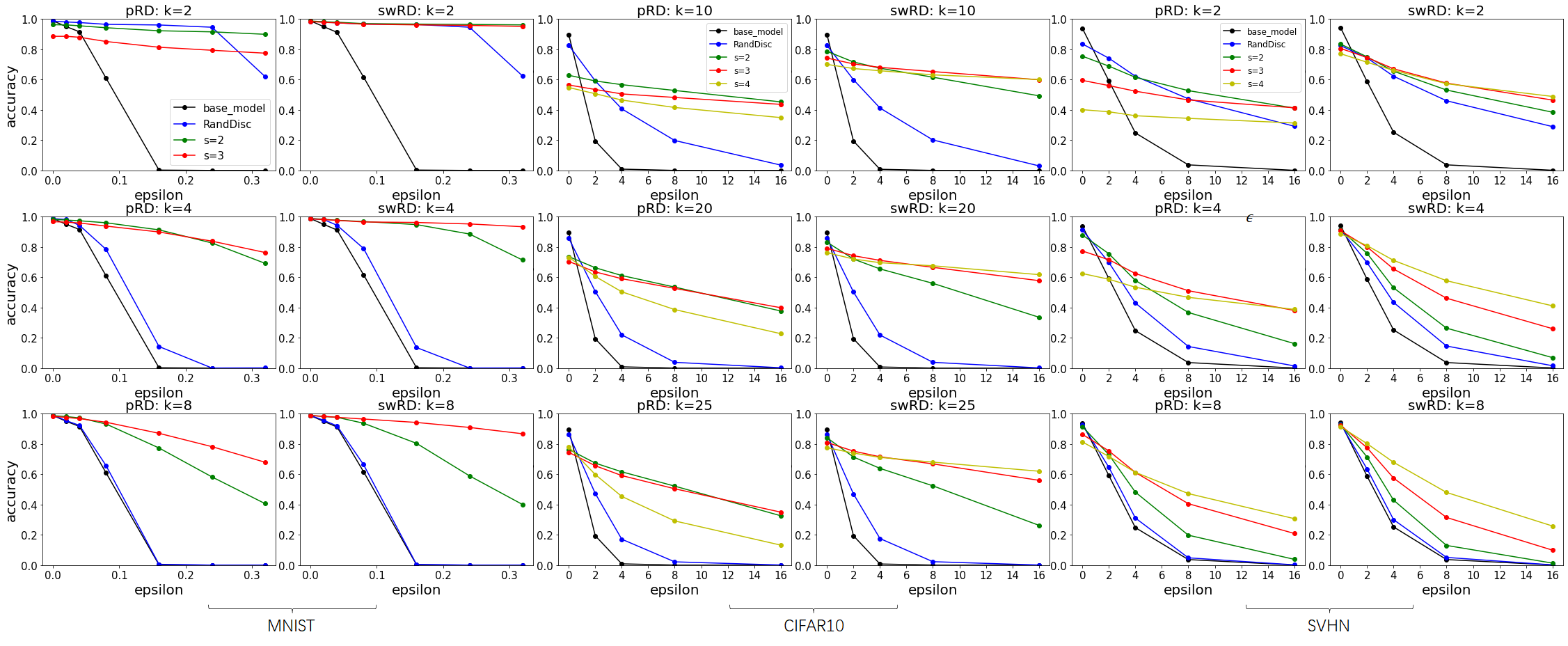
Figure 4: The accuracy of pRD and swRD against $\textrm{PGD}^{40}$ with different hyperparameters $s$ and $k$ on MNIST, CIFAR10 and SVHN.

Method	Params		Perturbation radius $\epsilon$
	$s$	$k$	$0$	$0.02$	$0.04$	$0.08$	$0.16$	$0.24$	$0.32$
Fast AdvT	-	-	98.63	98.12	97.60	96.77	91.44	87.69	71.76
MART	-	-	98.24	96.95	96.07	93.56	90.61	87.64	82.58
TRADES	-	-	97.59	96.68	95.45	93.15	88.86	78.14	41.46
RandDisc	1	2	98.57	98.07	97.67	96.51	96.08	94.56	62.09
pRD	2	2	96.26	96.12	95.54	94.26	92.26	91.55	89.94
swRD	2	2	98.80	98.28	97.56	96.77	96.76	96.52	95.59

Table 1: The accuracis (%) against $\textrm{PGD}^{40}$ with different sizes of perturbation on MNIST.

CIFAR10. The model $\mathbf{f}$ achieves 89.71% accuracy on the test set of CIFAR10. The attack is a 20-step PGD ($\textrm{PGD}^{20}$) with a step size $\alpha=\epsilon/10$. The noise level is set to $\sigma=\tau=4$ for both pRD and swRD, and the coefficient is $\beta=0.1$ in swRD. We also study the effects of the number of cluster centers $k$ and patch size $s$. The experimental results are summarized in Table 2 and the middle of Figure 4.

Method	Params		Perturbation radius $\epsilon$
	$s$	$k$	$0$	$2$	$4$	$8$	$16$
Fast AdvT	-	-	85.51	73.67	65.33	58.65	22.08
MART	-	-	83.07	74.25	65.39	57.57	32.19
TRADES	-	-	78.59	71.27	63.49	47.39	21.95
RandDisc	1	10	82.64	59.10	40.68	19.77	3.54
	1	20	85.77	50.61	21.78	3.82	0.24
	1	25	86.34	47.31	17.12	2.16	0.07
pRD	2	10	62.84	59.11	56.65	52.82	45.29
	2	20	73.65	66.31	61.17	53.51	37.78
swRD	3	25	81.03	75.32	71.46	66.88	56.03
	4	25	77.57	74.03	71.16	68.04	62.04

Table 2: The accuracis (%) against $\textrm{PGD}^{20}$ with different sizes of perturbation on CIFAR10.

SVHN. The model $\mathbf{f}$ achieves 94.24% accuracy on the validation set of SVHN. The attack is $\textrm{PGD}^{20}$, with a step size of $\alpha=\epsilon/10$. The noise level is set to $\sigma=\tau=4$ for both pRD and swRD, and the coefficient is $\beta=0.5$ in swRD. The results are presented in Table 3 and the right of Figure 4.

Method	Params		Perturbation radius $\epsilon$
	$s$	$k$	$0$	$2$	$4$	$8$	$16$
TRADES	-	-	86.54	65.55	57.60	42.70	21.78
RandDisc	1	2	83.57	74.11	62.22	47.31	29.18
	1	4	91.24	69.76	43.01	14.30	1.46
	1	8	93.45	63.48	30.03	5.09	0.14
pRD	2	2	75.46	68.89	61.51	52.72	41.20
	3	4	77.37	71.59	62.48	51.14	38.11
	4	8	81.37	71.76	61.30	47.26	30.70
swRD	4	2	77.12	71.43	66.12	57.28	48.87
	4	4	88.79	80.90	71.18	57.72	41.15
	4	8	91.45	80.22	67.91	48.02	25.84

Table 3: The accuracis (%) against $\textrm{PGD}^{20}$ with different sizes of perturbation on SVHN.

The experimental results show that for the MNIST dataset, our pRD defense exhibits greater robustness than the other methods when the perturbation size is large, while swRD consistently outperforms the other defenses. When $\epsilon$ is small, the robust accuracy of RandDisc is higher than that of pRD, and is close to that of swRD, which is in agreement with the outcomes of our theoretical experiments in Section 4.2. The results obtained on the CIFAR10 and SVHN datasets demonstrate a similar trend. That is, other defenses, especially RandDisc, have higher natural accuracy than our defenses. However, as the perturbation radius increases, the robust accuracy of our defenses becomes increasingly superior to that of other algorithms.

Figure 5: The robust accuracy of our defenses with different hyperparameters $\sigma$ and $\tau$ on SVHN. The attack is $\textrm{PGD}^{20}$ with $\epsilon=8$ (left) and $\textrm{PGD}^{20}$ with $\epsilon=16$(right).

We also study the impact of different parameters on accuracy of our defenses. Firstly, we observe that the number $k$ of cluster centers has a significant effect on the accuracy of our defenses, as illustrated in Figure 4. Specifically, increasing the value of $k$ leads to a rise in the natural accuracy of pRD and swRD, while their robust accuracy decreases, showing a trade-off between natural and robust accuracy. This trade-off is also observed in RandDisc. However, it can be alleviated by increasing the patch size (or window size) $s$. In other words, as the value of $k$ increases, increasing $s$ can improve both the natural accuracy and robustness of pRD and swRD. In addition, as shown in Figure 5, the noise level $\sigma$ and $\tau$ also impact the model performance. Specifically, pRD and swRD without any noise may achieve higher natural accuracy. However, introducing a suitable amount of noise can enhance the robustness of our defenses against attacks with large perturbation radius.

4.2 Certified accuracy via KL bound

In this subsection, we demonstrate that pRD and swRD have higher certified accuracy than RandDisc. As mentioned in Section 3.4, we measure the upper bounds on KL divergence of (6). To numerical obtain the value of this bound, we first defined a mapping from a set $C$ of centers to a vector $\overline{C}$ of centers: this mapping sorts all the elements in the center set in ascending order of their $\ell_{2}$ norm, and then concatenates them in a vector. By doing so, the complex computation of KL divergence between two distributions of random sets is converted into that of random vectors, which can be estimated numerically. Then we present the following Lemma:

Lemma 1. For a given clean image $x$ and its corresponding adversarial image $x^{\prime}$, consider a quantizer $\mathbf{Q}_{\hat{X}|X}^{\rm rPD}$ or $\mathbf{Q}_{\hat{X}|X}^{\rm swPD}$. The upper bound on the KL divergence between the output distribution of the quantizer for input $x$ and that for input $x^{\prime}$ is given by:

$${\rm D_{KL}}(\mathbf{Q}_{\hat{X}|X=x}^{\rm pRD}||\mathbf{Q}_{\hat{X}|X=x^{\prime}}^{\rm pRD})\leq{\rm D_{KL}}(\mathbf{Q}_{\overline{C}|X=x}^{\rm pRD}||\mathbf{Q}_{\overline{C}|X=x^{\prime}}^{\rm pRD})+\sum_{i=1}^{n}\mathbb{E}_{u\sim\mathbf{Q}_{C|X=x}^{\rm pRD}}[{\rm D_{KL}}(\mathbf{Q}_{\hat{P}_{i}|C=u,X=x}^{\rm pRD}||\mathbf{Q}_{\hat{P}_{i}|C=u,X=x^{\prime}}^{\rm pRD})]$$ (7)

$${\rm D_{KL}}(\mathbf{Q}_{\hat{X}|X=x}^{\rm swRD}||\mathbf{Q}_{\hat{X}|X=x^{\prime}}^{\rm swRD})\leq{\rm D_{KL}}(\mathbf{Q}_{\overline{C}|X=x}^{\rm swRD}||\mathbf{Q}_{\overline{C}|X=x^{\prime}}^{\rm swRD})+\sum_{i=1}^{n}\mathbb{E}_{u\sim\mathbf{Q}_{C|X=x}^{\rm swRD}}[{\rm D_{KL}}(\mathbf{Q}_{\hat{X}_{i}|C=u,X=x}^{\rm swRD}||\mathbf{Q}_{\hat{X}_{i}|C=u,X=x^{\prime}}^{\rm swRD})]$$ (8)

where $\hat{P}_{i}$ represents the $i$-th patch obtained in (1), and $\hat{X}_{i}$ represents the $i$-th pixel obtained in (4).

In practice, for each image and its corresponding adversarial image, we conduct 10,000 iterations of cluster center sampling, and then apply the above mapping to transform the resulting sets of cluster centers into vectors. To estimate the underlying distributions of these vectors, we utilize the Gaussian mixture model (GMM). However, given that there exists no closed-form expression for the KL divergence between two GMMs, we resort to Monte Carlo methods to estimate the divergence between two distributions $\mathbf{\hat{Q}}_{\overline{C}|X=x}$ and $\mathbf{\hat{Q}}_{\overline{C}|X=x^{\prime}}$:

$${\rm D_{KL}}(\mathbf{\hat{Q}}_{\overline{C}|X=x} ||\mathbf{\hat{Q}}_{\overline{C}|X=x^{\prime}})=E_{u\sim\mathbf{\hat{Q}}_{\overline{C}|X=x}}[\log\mathbf{\hat{Q}}_{\overline{C}|X=x} (u)-\log\mathbf{\hat{Q}}_{\overline{C}|X=x^{\prime}}(u)]$$ (9)

To approximate the expectation in equation (9), we draw 100,000 samples from the estimated distribution $\mathbf{\hat{Q}}_{\overline{C}|X=x}$, which we then average. For the second term on the right-hand side of (7) and (8), we utilize a similar method to estimate the distribution of each patch or pixel and subsequently compute the KL divergence. Notably, our experiments indicate that the magnitude of the second term is negligibly small (approximately $1e-5$) in comparison to that of the first term, rendering it inconsequential. Therefore, we evaluate the KL divergence between the distributions of cluster centers on the MNIST and CIFAR10 datasets. To this end, we use the naturally well-trained ResNet18 model and set the hyperparameters to $s=2$, $k=4$, and $\sigma=\tau=4$ for MNIST and $s=2$, $k=10$, and $\sigma=\tau=4$ for CIFAR10. In addition, the estimated values of KL divergence are highly sensitive to the number $k_{gmm}$ of clusters used in GMM, leading to significantly different ranges of resulting values. Here we select $k_{gmm}=2$ for all three defenses on MNIST and $k_{gmm}=8$ for all three defenses on CIFAR10.

Figure 6: The comparison of ${\rm D_{KL}}(\mathbf{\hat{Q}}_{\overline{C}|X=x}||\mathbf{\hat{Q}}_{\overline{C}|X=x^{\prime}})$ for RandDisc with that for our defenses on MNIST and CIFAR10. The results are shown in the left, and the right figures provide a zoomed-in view of a small perturbation range.

The results are depicted in Figure 6. For small perturbation size, RandDisc exhibits a lower KL divergence. However, as the perturbation radius $\epsilon$ increases, the KL divergences ${\rm D_{KL}}(\mathbf{\hat{Q}}_{\overline{C}|X=x}||\mathbf{\hat{Q}}_{\overline{C}|X=x^{\prime}})$ for pRD and swRD are much lower than that in RandDisc on both MNIST and CIFAR10. This observation suggests that RandDisc may achieve higher certified accuracy than our proposed defenses under small perturbations, but as the perturbation level increases, the certified accuracy of RandDisc will substantially decrease and become much lower than that of our defenses for large values of $\epsilon$. These empirical findings and our corresponding explanation are supported by the experiments on robust accuracy presented in Section 4.1.

4.3 Denoising Effects

Figure 7: The examples of quantized images by RandDisc, pRD, and swRD. The first and third rows show the clean images $x$ and their quantized versions $\hat{x}$, the second and fourth rows show the corresponding adversarial images $x^{\prime}$ and their quantized versions $\hat{x}^{\prime}$. In MNIST, the number of cluster centers $k$ is $2$, and the patch/window size $s$ of pRD and swRD is $2$, while in CIFAR10, the number of cluster centers $k$ is $25$, and the patch/window size $s$ of pRD and swRD is $2$.

Visual inspection of the quantized images reveals remarkable denoising effects of the proposed defense, particularly swRD. Figure 7 presents several example images quantized by RandDisc, pRD, and swRD.

For MNIST, the adversarial examples $x^{\prime}$ are generated by $\textrm{PGD}^{40}$ with $\epsilon=0.32$, while for CIFAR10, they are generated by $\textrm{PGD}^{20}$ with $\epsilon=16$. First, it can be found that the quantized clean image $\hat{x}$ and the quantized adversarial image $\hat{x}^{\prime}$ of our defenses, especially of swRD, are much closer than those of RandDisc. This finding suggests that our KL divergence between $\mathbf{Q}_{\hat{X}|X=x}$ and $\mathbf{Q}_{\hat{X}|X=x^{\prime}}$ may be much smaller than RandDisc. These visual results are consistent with our empirical and theoretical findings in Section 4.1 and 4.2.

In addition, we observe that the quantized adversarial image $\hat{x}^{\prime}$ produced by swRD is remarkably similar to the clean image $x$. As a result, swRD can be viewed as a denoiser that removes adversarial noise from $x^{\prime}$ to produce $x$. Unlike the defensive denoisers in previous works [34, 13, 19, 11], swRD does not use any information from the original image $x$, nor does it train an extra network to learn the relationship between $x$ and $x^{\prime}$. The input of swRD is solely the perturbed image $x^{\prime}$, and it shows superior performance with simpler computation.

4.4 Robust accuracy of t-pRD and t-swRD

Figure 8: The comparison of our methods using the $\mathbf{f}$ trained on natural dataset versus using the $\hat{\mathbf{f}}$ trained on quantized dataset. Left(CIFAR10): The accuracy of pRD and t-pRD with $s=2,k=10$, and the accuracy of sw-RD and t-swRD with $s=4,k=25$; Right(SVHN): The accuracy of pRD and t-pRD with $s=2,k=2$, and the accuracy of sw-RD and t-swRD with $s=4,k=2$.

We report experiments on a model $\hat{\mathbf{f}}$ that is trained on quantized CIFAR10 and SVHN datasets. Specifically, the model $\mathbf{f}$ in Figure 3 is trained on quantized training set by $\mathbf{Q}_{\hat{X}|X}^{\rm pRD}$ and $\mathbf{Q}_{\hat{X}|X}^{\rm swRD}$. Figure 8 illustrates the improvements in both natural and robust accuracy achieved by our training strategies, t-pRD and t-swRD, as compared to pRD and swRD, respectively. Notably, for the perturbation size of $\epsilon=16$ on SVHN, our defense t-swRD achieves an accuracy of 81.45%, which is 39.65% higher than that of swRD.

5 Conclusion

In this paper, we propose two defense strategies, pRD and swRD, using vector quantization in a high dimensional space. Our experiments on MNIST, CIFAR10, and SVHN demonstrate that our pRD and swRD achieve higher certified accuracy than RandDisc [38], and outperform other state-of-the-art defenses in terms of robust accuracy against PGD attacks. In particular, swRD functions as a denoiser, removing adversarial noise from adversarial examples with superior denoising ability and simpler computation than previous denoising approaches. We further improve pRD and swRD by training the classifier on a quantized dataset, resulting in t-pRD and t-swRD, respectively. Our experiments demonstrate that these strategies show significant improvements in both natural and robust accuracy. Therefore, increasing the accuracy of quantized clean images will enhance the likelihood of correctly classifying quantized perturbed images. As such, our future work will focus on improving the natural accuracy of pRD and swRD.

References

- [1] Naveed Akhtar and Ajmal Mian. Threat of adversarial attacks on deep learning in computer vision: A survey. Ieee Access, 6:14410–14430, 2018.
- [2] Wieland Brendel, Jonas Rauber, and Matthias Bethge. Decision-based adversarial attacks: Reliable attacks against black-box machine learning models. arXiv preprint arXiv:1712.04248, 2017.
- [3] Nicholas Carlini and David Wagner. Towards evaluating the robustness of neural networks. In 2017 ieee symposium on security and privacy (sp), pages 39–57. Ieee, 2017.
- [4] Pin-Yu Chen, Huan Zhang, Yash Sharma, Jinfeng Yi, and Cho-Jui Hsieh. Zoo: Zeroth order optimization based black-box attacks to deep neural networks without training substitute models. In Proceedings of the 10th ACM workshop on artificial intelligence and security, pages 15–26, 2017.
- [5] Jeremy Cohen, Elan Rosenfeld, and Zico Kolter. Certified adversarial robustness via randomized smoothing. In international conference on machine learning, pages 1310–1320. PMLR, 2019.
- [6] Gintare Karolina Dziugaite, Zoubin Ghahramani, and Daniel M Roy. A study of the effect of jpg compression on adversarial images. arXiv preprint arXiv:1608.00853, 2016.
- [7] Ian J Goodfellow, Jonathon Shlens, and Christian Szegedy. Explaining and harnessing adversarial examples. arXiv preprint arXiv:1412.6572, 2014.
- [8] Shixiang Gu and Luca Rigazio. Towards deep neural network architectures robust to adversarial examples. arXiv preprint arXiv:1412.5068, 2014.
- [9] Chuan Guo, Mayank Rana, Moustapha Cisse, and Laurens Van Der Maaten. Countering adversarial images using input transformations. arXiv preprint arXiv:1711.00117, 2017.
- [10] Ruitong Huang, Bing Xu, Dale Schuurmans, and Csaba Szepesvári. Learning with a strong adversary. arXiv preprint arXiv:1511.03034, 2015.
- [11] Xiaojun Jia, Xingxing Wei, Xiaochun Cao, and Hassan Foroosh. Comdefend: An efficient image compression model to defend adversarial examples. In Proceedings of the IEEE/CVF conference on computer vision and pattern recognition, pages 6084–6092, 2019.
- [12] Alexey Kurakin, Ian Goodfellow, and Samy Bengio. Adversarial machine learning at scale. arXiv preprint arXiv:1611.01236, 2016.
- [13] Fangzhou Liao, Ming Liang, Yinpeng Dong, Tianyu Pang, Xiaolin Hu, and Jun Zhu. Defense against adversarial attacks using high-level representation guided denoiser. In Proceedings of the IEEE conference on computer vision and pattern recognition, pages 1778–1787, 2018.
- [14] Aleksander Madry, Aleksandar Makelov, Ludwig Schmidt, Dimitris Tsipras, and Adrian Vladu. Towards deep learning models resistant to adversarial attacks. arXiv preprint arXiv:1706.06083, 2017.
- [15] Dongyu Meng and Hao Chen. Magnet: a two-pronged defense against adversarial examples. In Proceedings of the 2017 ACM SIGSAC conference on computer and communications security, pages 135–147, 2017.
- [16] Seyed-Mohsen Moosavi-Dezfooli, Alhussein Fawzi, Omar Fawzi, and Pascal Frossard. Universal adversarial perturbations. In Proceedings of the IEEE conference on computer vision and pattern recognition, pages 1765–1773, 2017.
- [17] Seyed-Mohsen Moosavi-Dezfooli, Alhussein Fawzi, and Pascal Frossard. Deepfool: a simple and accurate method to fool deep neural networks. In Proceedings of the IEEE conference on computer vision and pattern recognition, pages 2574–2582, 2016.
- [18] Nina Narodytska and Shiva Prasad Kasiviswanathan. Simple black-box adversarial perturbations for deep networks. arXiv preprint arXiv:1612.06299, 2016.
- [19] Muzammal Naseer, Salman Khan, Munawar Hayat, Fahad Shahbaz Khan, and Fatih Porikli. A self-supervised approach for adversarial robustness. In Proceedings of the IEEE/CVF Conference on Computer Vision and Pattern Recognition, pages 262–271, 2020.
- [20] Nicolas Papernot, Patrick McDaniel, Ian Goodfellow, Somesh Jha, Z Berkay Celik, and Ananthram Swami. Practical black-box attacks against machine learning. In Proceedings of the 2017 ACM on Asia conference on computer and communications security, pages 506–519, 2017.
- [21] Nicolas Papernot, Patrick McDaniel, Somesh Jha, Matt Fredrikson, Z Berkay Celik, and Ananthram Swami. The limitations of deep learning in adversarial settings. In 2016 IEEE European symposium on security and privacy (EuroS&P), pages 372–387. IEEE, 2016.
- [22] Nicolas Papernot, Patrick McDaniel, Xi Wu, Somesh Jha, and Ananthram Swami. Distillation as a defense to adversarial perturbations against deep neural networks. In 2016 IEEE symposium on security and privacy (SP), pages 582–597. IEEE, 2016.
- [23] Aditi Raghunathan, Jacob Steinhardt, and Percy Liang. Certified defenses against adversarial examples. arXiv preprint arXiv:1801.09344, 2018.
- [24] Leslie Rice, Eric Wong, and Zico Kolter. Overfitting in adversarially robust deep learning. In International Conference on Machine Learning, pages 8093–8104. PMLR, 2020.
- [25] Andrew Ross and Finale Doshi-Velez. Improving the adversarial robustness and interpretability of deep neural networks by regularizing their input gradients. In Proceedings of the AAAI Conference on Artificial Intelligence, volume 32, 2018.
- [26] Swami Sankaranarayanan, Arpit Jain, Rama Chellappa, and Ser Nam Lim. Regularizing deep networks using efficient layerwise adversarial training. In Proceedings of the AAAI Conference on Artificial Intelligence, volume 32, 2018.
- [27] Claude E Shannon et al. Coding theorems for a discrete source with a fidelity criterion. IRE Nat. Conv. Rec, 4(142-163):1, 1959.
- [28] Christian Szegedy, Wojciech Zaremba, Ilya Sutskever, Joan Bruna, Dumitru Erhan, Ian Goodfellow, and Rob Fergus. Intriguing properties of neural networks. arXiv preprint arXiv:1312.6199, 2013.
- [29] Sergei Vassilvitskii and David Arthur. k-means++: The advantages of careful seeding. In Proceedings of the eighteenth annual ACM-SIAM symposium on Discrete algorithms, pages 1027–1035, 2006.
- [30] Yisen Wang, Difan Zou, Jinfeng Yi, James Bailey, Xingjun Ma, and Quanquan Gu. Improving adversarial robustness requires revisiting misclassified examples. In International Conference on Learning Representations, 2020.
- [31] Eric Wong and Zico Kolter. Provable defenses against adversarial examples via the convex outer adversarial polytope. In International conference on machine learning, pages 5286–5295. PMLR, 2018.
- [32] Eric Wong, Leslie Rice, and J Zico Kolter. Fast is better than free: Revisiting adversarial training. arXiv preprint arXiv:2001.03994, 2020.
- [33] Cihang Xie, Jianyu Wang, Zhishuai Zhang, Zhou Ren, and Alan Yuille. Mitigating adversarial effects through randomization. arXiv preprint arXiv:1711.01991, 2017.
- [34] Cihang Xie, Yuxin Wu, Laurens van der Maaten, Alan L Yuille, and Kaiming He. Feature denoising for improving adversarial robustness. In Proceedings of the IEEE/CVF conference on computer vision and pattern recognition, pages 501–509, 2019.
- [35] Weilin Xu, David Evans, and Yanjun Qi. Feature squeezing: Detecting adversarial examples in deep neural networks. arXiv preprint arXiv:1704.01155, 2017.
- [36] Bohang Zhang, Tianle Cai, Zhou Lu, Di He, and Liwei Wang. Towards certifying robustness using neural networks with l-dist neurons. arXiv preprint arXiv:2102.05363, 2021.
- [37] Hongyang Zhang, Yaodong Yu, Jiantao Jiao, Eric Xing, Laurent El Ghaoui, and Michael Jordan. Theoretically principled trade-off between robustness and accuracy. In International conference on machine learning, pages 7472–7482. PMLR, 2019.
- [38] Yuchen Zhang and Percy Liang. Defending against whitebox adversarial attacks via randomized discretization. In The 22nd International Conference on Artificial Intelligence and Statistics, pages 684–693. PMLR, 2019.