The Green Bank North Celestial Cap Survey. VIII. 21 New Pulsar Timing Solutions

Abstract

We present timing solutions for 21 pulsars discovered in 350 MHz surveys using the Green Bank Telescope (GBT). All were discovered in the Green Bank North Celestial Cap pulsar survey, with the exception of PSR J0957$-$0619, which was found in the GBT 350 MHz Drift-scan pulsar survey. The majority of our timing observations were made with the GBT at 820 MHz. With a spin period of 37 ms and a 528-day orbit, PSR J0032+6946 joins a small group of five other mildly recycled wide binary pulsars, for which the duration of recycling through accretion is limited by the length of the companion’s giant phase. PSRs J0141+6303 and J1327+3423 are new disrupted recycled pulsars. We incorporate Arecibo observations from the NANOGrav pulsar timing array into our analysis of the latter. We also observed PSR J1327+3423 with the Long Wavelength Array, and our data suggest a frequency-dependent dispersion measure. PSR J0957$-$0619 was discovered as a rotating radio transient, but is a nulling pulsar at 820 MHz. PSR J1239+3239 is a new millisecond pulsar (MSP) in a 4-day orbit with a low-mass companion. Four of our pulsars already have published timing solutions, which we update in this work: the recycled wide binary PSR J0214+5222, the non-eclipsing black widow PSR J0636+5128, the disrupted recycled pulsar J1434+7257, and the eclipsing binary MSP J1816+4510, which is in an 8.7 hr orbit with a redback-mass companion.

1 Introduction

The Green Bank North Celestial Cap (GBNCC) survey uses the Green Bank Telescope (GBT) to search for new pulsars at a radio frequency of 350 MHz. Since the beginning of the survey in 2009, it has made 124,852 observations, each 120 s in duration, covering the entire GBT sky (declination $\delta>-40\arcdeg$). To date, GBNCC has discovered 194 pulsars. The current sky coverage of the survey is shown in Figure 1. In the coming months, the survey will be fully completed, as pointings which were rendered unusable by radio-frequency interference (RFI) are re-observed.

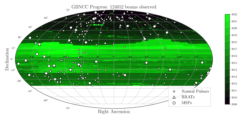
Figure 1: A skymap showing the GBNCC survey’s sky coverage and its discoveries, which are differentiated between normal (“slow”) pulsars, rotating radio transients (RRATs), and millisecond pulsars (MSPs). Each pointing is colored based on the date on which it was observed.

Survey observations use the Green Bank Ultimate Pulsar Processing Instrument (GUPPI; Ransom et al., 2009) to sample the 100 MHz bandwidth, which is split into 4096 frequency channels, once every 81.92 $\mu$s. Data are processed on Compute Canada supercomputers at McGill University, using a searching pipeline which makes use of the pulsar searching software package PRESTO (Ransom et al., 2002). Candidate periodic and single-pulse signals are inspected by eye (often by undergraduate students), and promising candidates are followed up with the GBT. Candidates which are confirmed as pulsars must be regularly observed over the course of a year to reach a phase-connected timing solution, which fully describes a pulsar’s astrometric, rotational, and orbital parameters.

For a comprehensive overview and description of the GBNCC pulsar survey and its goals, as well as initial timing solutions for PSRs J0214+5222, J0636+5128, J1434+7257, and J1816+4510, which we are updating in this work, see Stovall et al. (2014). Timing solutions for other GBNCC pulsar discoveries appear in Kaplan et al. (2012), Karako-Argaman et al. (2015), Kawash et al. (2018), Lynch et al. (2018), Aloisi et al. (2019), Agazie et al. (2021), and Swiggum et al. (2023). The first GBNCC FRB discovery was reported in Parent et al. (2020). A census of the survey’s discoveries and an analysis of its sensitivity can be found in McEwen et al. (2020). The survey maintains a website listing its discoveries and showing its current progress, as well as a Github page which provides published standard profiles, pulse times of arrival, and timing models from many of the above studies.

The main goal of the GBNCC survey is to discover new millisecond pulsars (MSPs). Pulsars lose rotational energy over time, “spinning down” until radio emission ceases. These old neutron stars sometimes go through a period of accretion from a binary companion. This process, known as recycling, transfers angular momentum to the neutron star. If recycling is allowed to proceed uninterrupted, pulsars are spun up to $\sim$ ms spin periods. This process also reduces the strength of the pulsar’s surface magnetic field (Alpar et al., 1982). Due to their extremely stable rotation, MSPs have high timing precision which can rival that of terrestrial atomic clocks (Hobbs et al., 2012, 2020). This precision can be exploited to study a wide range of astrophysical phenomena, including tests of general relativity (see, e.g., Archibald et al., 2018; Kramer et al., 2021), constraining the neutron star equation of state by measuring pulsar masses (Cromartie et al., 2020; Fonseca et al., 2021), and pulsar formation mechanisms and evolution.

By finding MSPs with sufficient timing precision, surveys like GBNCC are able to provide critical additions to pulsar timing array (PTA) experiments, which are Galaxy-sized gravitational wave (GW) detectors composed of many Earth–pulsar “arms,” sensitive to GWs at nanohertz frequencies. The first hints of a nanohertz GW background may be present in the 12.5-year data set of the North American Nanohertz Observatory for Gravitational waves (NANOGrav; Alam et al., 2021), the North American PTA. Similar hints of a signal are also present in the most recent International Pulsar Timing Array (IPTA) data release (Perera et al., 2019; Antoniadis et al., 2022), which combined data sets from PTAs in Australia (Parkes Pulsar Timing Array, PPTA), Europe (European Pulsar Timing Array, EPTA), and North America. Eleven GBNCC discoveries have been observed by PTAs, including two pulsars in this analysis: PSR J0636+5128, which is currently observed by NANOGrav and the European PTA; and PSR J1327+3423, which was observed by NANOGrav until operations at the 305-m Arecibo radio telescope were suspended a few months prior to the tragic collapse of the telescope in December 2020. When NANOGrav’s timing program was transferred entirely to the GBT, observations of PSR J1327+3423 were discontinued.

Additional goals for the GBNCC survey include discovering new nulling pulsars and rotating radio transients (RRATs; McLaughlin et al., 2006); exotic binary systems such as double neutron star (DNS) systems, black widows and redbacks Fruchter et al. (1988); Roberts (2011); and studying the Galactic pulsar population as a whole. Black widows and redbacks, collectively known as “spider” binaries, are MSPs in short, $P_{\mathrm{b}}\lesssim 1$ day orbits. In these systems, the companion is ablated by the energetic pulsar wind, releasing ionized material into the system, which smears and delays the pulsar’s radio pulses or causes radio eclipses (Polzin et al., 2018). Spiders have a bimodal distribution of companion masses, with black widows having $M_{\mathrm{c}}\lesssim 0.05$ M_☉ and redbacks having $M_{\mathrm{c}}\gtrsim 0.1$ M_☉ (Chen et al., 2013).

Recycled pulsars which are neither MSPs nor in binary systems are known as disrupted recycled pulsars (DRPs), defined by Belczynski et al. (2010) as isolated pulsars in the Galactic disc (i.e., not in a globular cluster, where many-body interactions can easily disrupt binary systems) with spin periods of $P>20$ ms, and low surface magnetic fields, $B_{\mathrm{surf}}<3\times 10^{10}\,\textrm{G}$. These properties suggest that such a DRP was in the process of accreting from a binary companion when that companion underwent a supernova explosion, imparting a kick that disrupted the binary. This may result in larger space velocities for DRPs compared to other pulsar populations, such as DNS binaries (Lorimer et al., 2004). This picture of pulsar evolution can be tested by, e.g., comparing the relative numbers and/or space velocities of DNS systems and DRPs (Kawash et al., 2018).

We note that one of the pulsars in this analysis, PSR J1913+3732, was reported as a discovery in the HTRU-North survey, a pulsar survey at 1.36 GHz with the Effelsberg radio telescope (Barr et al., 2013). That paper also includes a timing solution for this pulsar with parameters consistent with, and comparable in precision to, those presented in this work. In this work, we present our own independent pulse profiles, flux density measurements, and timing solution for this pulsar.

In Section 2, we describe our timing observations of 21 pulsars. We present pulse profiles, estimated flux densities, and spectral indices in Section 3 and describe our timing analysis in Section 4. In Section 5, we present our timing solutions and discuss some individual systems. We conclude with Section 6.

2 Pulsar Timing Observations

The discoveries and initial timing follow-up observations of PSRs J0214+5222, J0636+5128, J1434+7257, and J1816+4510 were detailed in Stovall et al. (2014). We refer to that work for detailed descriptions of those observations (which were made with the GBT at 350, 820, 1500, and 2000 MHz), describing all new timing observations here. The pulsars in this analysis were each discovered as periodicity candidates in GBNCC survey observations, except for PSR J0957$-$0619, which was discovered in a search for single pulses in the 350 MHz GBT Drift-scan survey (Karako-Argaman et al., 2015).

After confirmation with the GBT at 350 MHz, many of the pulsars in this analysis were used as test sources during regular survey observing. Observations of known pulsars as test sources are performed during each survey observing session to ensure data quality and monitor the RFI environment. These test scans use the same observing set up as usual survey observations: the 100 MHz bandwidth, centered at 350 MHz, is split into 4096 frequency channels, with a sampling time of 81.92 $\mu$s. A small number of test source observations used in our timing analysis were made with the newer VEGAS backend instead of GUPPI, using an identical setup.

At 350 MHz, the GBT beam has a FWHM of 36′, so the sky positions of recently-confirmed pulsars are not precisely known. This can cause difficulty in reaching a timing solution, and can significantly reduce the signal-to-noise ratio (S/N) of timing observations, as the 820 MHz beam is only $7\arcmin$ wide. To ameliorate this issue, pulsar positions were refined using the traditional gridding technique. For each pulsar, six observations were made sequentially, each at 820 MHz, with 200 MHz bandwidth split into 2048 channels and 40.96 $\mu$s time resolution. These gridding beams were distributed evenly across the 350 MHz discovery beam. The varying S/N at each sky location allows the inference of an improved pulsar position. As long as the gaps between our timing follow-up observations of a pulsar and any discovery, test source, and gridding observations were short enough, such that phase connection could be maintained, we used them in our timing analysis.

After localization, pulsars were observed once monthly for a year at the GBT (project code 15A-376; PI: L. Levin) at 820 MHz. Each pulsar had at least one period of high cadence observing, with 4 – 5 observations made within a period of one week, to facilitate phase connection and the solving of orbital parameters, if applicable. Timing solutions were not available for many pulsars at the outset of the timing campaign, so the majority of our observations were not coherently folded or dedispersed (“search-mode” data, which have the same configuration as the gridding scans described previously). For a few pulsars, a suitable timing ephemeris was available, so data were coherently dedispersed to the correct DM and folded on the pulsar’s spin period (“fold-mode” data), using 2048 phase bins and 10 s sub-integrations. Raw fold-mode data contained polarization information, and polarization calibration scans were taken, but we leave a polarization analysis of these pulsars to a future work.

Some pulsars were also observed under two similar GBT timing campaigns, each lasting $\sim$1 yr: one using the same setup at 820 MHz (project code 17B-285; PI: J. Swiggum), the other observing at 350 MHz (project code 16A-343; PI: M. DeCesar). Once again, search mode was used for some pulsars, with a setup at 350 MHz identical to GBNCC survey observations, and fold mode for others. With the 350 MHz receiver, fold mode uses 128 frequency channels and a 1.28 $\mu$s sampling time.

We observed PSR J0214+5222 with the Low Frequency Array (LOFAR) at 149 MHz, under project number LC0_002. These observations are described in detail in Lynch et al. (2018); Kondratiev et al. (2016). Data were recorded using 78.125 MHz of bandwidth split into 400 subbands, each split into 16 channels with a sampling time of 327.68 $\mu$s.

We also used the Long Wavelength Array (LWA) to observe PSR J1327+3423 approximately once every three weeks between MJDs 56863 (2014 September) and 57869 (2017 April). Observations were made with the LWA Station 1 (LWA1). The LWA1 (Ellingson et al., 2013) is capable of forming four independently-steerable beams, each with two independently-selectable center frequencies with up to 19.6 MHz of bandwidth each (due to rolloffs in sensitivity towards the edges of the band, the usable bandwidth per tunable center frequency is $\sim$ 16 MHz). Most of our observations used two beams, one with center frequencies at 35.1 and 49.8 MHz, and another with 64.5 and 79.2 MHz, using the maximum bandwidth available. On some epochs, PSR J1327+3423 was only observed with one beam, and thus at only two frequencies, but these were chosen such that each portion of the band was observed a total of 41 times, except for 49.8 MHz, which was observed 40 times. Data were coherently dedispersed and folded (30 s duration sub-integrations) using a real-time spectrometer with a sampling time of 81.08 $\mu$s. Each beam had 1024 frequency channels available, so the bands corresponding to each center frequency were each split into 512 channels, resulting in a channel bandwidth of $\approx$ 38.3 kHz.

Observations of PSR J1327+3423 by the NANOGrav PTA, using the 305-m William E. Gordon radio telescope at Arecibo Observatory (AO), were made available to GBNCC. This is in accordance with the data-sharing agreement between major pulsar surveys and PTAs, whereby the surveys share timing ephemerides of high-timing-precision MSP discoveries with PTAs, and the PTAs share timing products with the surveys. AO observations of this pulsar were taken in the same manner as described in NANOGrav Collaboration et al. (2015), but we summarize them here. Observations were made at $\sim$ monthly cadence, at center frequencies 430 and 1380 MHz, with an observation with one receiver followed immediately by an observation with the other within $\sim$1 hr, accompanied by measurements of pulsed noise diode signals to calibrate the polarization response of the receiver. Most observations were 19 min in duration, with a few as short as 10 min and the longest at 40 min. Data were recorded by the Puerto Rican Ultimate Pulsar Processing Instrument (PUPPI; nearly identical to GUPPI) pulsar backend with a sampling time of 64 $\mu$s, and 1.5625 MHz-wide frequency channels, with a bandwidth of 24 and 800 MHz for the 430 and 1380 MHz receivers, respectively. Observations were folded and dedispersed coherently using the pulsar ephemeris and DM, resulting in data products with 10 s sub-integrations and 2048 pulse phase bins.

3 Pulse Profiles, Flux Densities, and Spectral Indices

We estimate flux densities $S_{\nu}$ for each pulsar at each observing band’s central radio frequency $\nu$ using the radiometer equation as presented in Lorimer & Kramer (2004):

$$S_{\nu}=\beta\,\frac{(\mathrm{S/N})\,T_{\mathrm{sys}}}{G\,\sqrt{n_{\mathrm{p}}\,t_{\mathrm{int}}\,\Delta\nu}}\,\sqrt{\frac{\delta}{1-\delta}}.$$ (1)

Here, $\beta=1.3$ is a degradation factor due to digitization, S/N is the signal-to-noise ratio, $T_{\mathrm{sys}}$ is the system temperature, $G$ is the telescope gain, $n_{\mathrm{p}}=2$ is the number of polarizations, $t_{\mathrm{int}}$ is the total integration time on source, $\Delta\nu$ is the effective bandwidth, and $\delta$ is the pulse duty cycle. S/N was measured from the summed pulse profiles shown in Figures 2 and 3. We calculated equivalent widths $W_{\mathrm{eq}}$ for each pulse profile, defined in Lorimer & Kramer (2004) as the width of a boxcar pulse with the same area and peak height as the pulse profile. The duty cycle is then $\delta=W_{\mathrm{eq}}/P$. We report $\delta$ and $W_{\mathrm{eq}}/P$ for each pulsar in Table 1; we did not add together the LWA1 bands and instead report distinct measurements at 35.1, 49.8, 64.5, and 79.2 MHz for PSR J1327+3423 in Table 2.

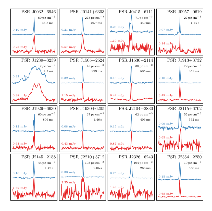
Figure 2: Summed pulse profiles for 16 of the pulsars in this analysis. Each profile has been normalized to the same peak height, shows the emission from one full rotation of the pulsar, and is divided into 128 bins. They were generated using all GBT data which were within the degradation tolerances described in Section 3. We show 350 MHz profiles in red and 820 MHz profiles above them in blue. Below each pulsar’s name, we give its DM and spin period.

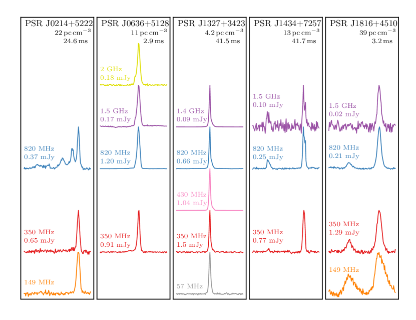
Figure 3: Summed pulse profiles for the five pulsars in this analysis which were observed at additional telescopes/frequencies. Each profile has been normalized to the same peak height, shows the emission from one full rotation of the pulsar, and is divided into 128 bins. They were generated from all data which were within the degradation tolerances described in Section 3. The telescopes used were LWA1 (57 MHz), LOFAR (149 MHz), GBT (350, 820, 1500, and 2000 MHz), and AO (430 and 1380 MHz). We also show the 149 MHz LOFAR profile of PSR J1816+4510, which is the same profile shown in Stovall et al. (2014). The center frequency of the observations used to generate each profile and the estimated flux density $S_{\nu}$ at that frequency are listed to the left of each profile. We did not estimate $S_{\nu}$ from LOFAR profiles, and we estimated $S_{\nu}$ separately for each LWA1 subband, so we do not list $S_{\nu}$ estimates beside those profiles. Below each pulsar’s name, we give its DM and spin period.

Table 1: Duty Cycles & Equivalent Pulse Widths of GBNCC Pulsars

	149 MHz		350 MHz		430 MHz		820 MHz		1380/1500 MHz		2000 MHz
PSR	$\delta$	$W_{\mathrm{eq}}$	$\delta$	$W_{\mathrm{eq}}$	$\delta$	$W_{\mathrm{eq}}$	$\delta$	$W_{\mathrm{eq}}$	$\delta$	$W_{\mathrm{eq}}$	$\delta$	$W_{\mathrm{eq}}$
	(%)	(ms)	(%)	(ms)	(%)	(ms)	(%)	(ms)	(%)	(ms)	(%)	(ms)
J0032+6946	…	…	03.84	001.420	…	…	02.23	000.820	…	…	…	…
J0141+6303	…	…	05.07	002.370	…	…	02.78	001.300	…	…	…	…
J0214+5222	5.81	1.428	04.37	001.075	…	…	21.32	005.240	…	…	…	…
J0415+6111	…	…	04.40	019.400	…	…	04.34	019.100	…	…	…	…
J0636+5128	…	…	04.76	000.136	…	…	04.97	000.143	5.58	0.16	5.42	0.156
J0957$-$0619	…	…	00.51	008.800	…	…	01.97	034.000	…	…	…	…
J1239+3239	…	…	24.63	001.158	…	…	34.07	001.602	…	…	…	…
J1327+3423	…	…	02.90	001.200	3.0	1.25	03.03	001.260	2.83	1.18	…	…
J1434+7257	…	…	08.31	003.470	…	…	09.71	004.050	8.86	3.7	…	…
J1505$-$2524	…	…	01.85	018.500	…	…	02.20	021.900	…	…	…	…
J1530$-$2114	…	…	02.62	013.200	…	…	02.60	013.100	…	…	…	…
J1816+4510	54.1	1.728	26.24	000.838	…	…	18.29	000.584	6.3	0.201	…	…
J1913+3732	…	…	02.03	017.300	…	…	01.98	016.800	…	…	…	…
J1929+6630	…	…	02.74	022.100	…	…	02.08	016.800	…	…	…	…
J1930+6205	…	…	01.52	022.200	…	…	01.40	020.300	…	…	…	…
J2104+2830	…	…	01.87	007.600	…	…	01.62	006.600	…	…	…	…
J2115+6702	…	…	03.75	020.700	…	…	04.46	024.600	…	…	…	…
J2145+2158	…	…	02.63	037.400	…	…	02.21	031.300	…	…	…	…
J2210+5712	…	…	05.94	122.000	…	…	02.18	044.800	…	…	…	…
J2326+6243	…	…	05.05	013.400	…	…	03.59	009.500	…	…	…	…
J2354$-$2250	…	…	02.45	013.700	…	…	02.85	015.900	…	…	…	…

Note. — Pulse duty cycles $\delta$ and widths $W_{\mathrm{eq}}$ of a boxcar pulse with equivalent height to the peak height of the pulse profile are listed for each pulsar in this analysis. The telescopes used were LOFAR (149 MHz), GBT (350, 820, 1500, and 2000 MHz), and AO (430 and 1380 MHz). Measurements made at L-band (1380 MHz with AO and 1500 MHz with the GBT) are listed in the same column, with the 1380 MHz measurements italicized.

Table 2: LWA1 Pulse Widths & Flux Densities for PSR J1327+3423

$\nu$	$t_{\mathrm{int}}$	$\delta$	$W_{\mathrm{eq}}$	$S_{\nu}$
(MHz)	(s)	(%)	(ms)	(mJy)
35.1	14437	3.45	1.43	80(50)
49.8	61508	3.41	1.42	2.1(1.3)$\times$102
64.5	57802	2.87	1.19	2.0(1.3)$\times$102
79.2	57802	2.47	1.02	1.8(1.1)$\times$102

Note. — At each center frequency $\nu$, the total integration time $t_{\mathrm{int}}$, pulse duty cycle $\delta$, width $W_{\mathrm{eq}}$ (that of a boxcar pulse with equivalent height to the peak height of the pulse profile), and estimated flux density $S_{\nu}$ are shown for PSR J1327+3423. Values in parentheses are uncertainties, estimated as described in Section 3.

To ensure we account for persistent sources of RFI and rolloffs in sensitivity at the edges of the band, we assumed $\Delta\nu=90$% of the true observing bandwidth. We reduced this to 75% for AO observations at 1380 MHz due to increased RFI. In 2014, a new source of strong, persistent RFI rendered GBT data in the range 360 – 380 MHz unusable. This has caused a $\approx$20% reduction in the effective bandwidth of the 350 MHz receiver. For pulsars with 350 MHz observations both before and after the change, we took $\Delta\nu_{350}=80\,\textrm{MHz}$. Observations of PSR J0141+6303 at 350 MHz only occurred after this source of RFI appeared, so we took $\Delta\nu_{350}=70\,\textrm{MHz}$.

The system temperature $T_{\mathrm{sys}}=T_{\mathrm{rec}}+T_{\mathrm{sky}}$, where $T_{\mathrm{rec}}$ is the receiver temperature and $T_{\mathrm{sky}}$ is the position-dependent sky temperature, including contribution from the cosmic microwave background. Referencing the GBT Proposer’s Guide, we took $T_{\mathrm{rec}}$ to be 23, 22, 20, and 18 K, at 350, 820, 1500, and 2000 MHz, respectively. From the Arecibo 305-m telescope User’s Guide, $T_{\mathrm{rec}}=35$ and 25 K at 430 and 1380 MHz, respectively. We used pyGDSM, a Python interface for Zheng et al. (2017)’s global sky model of diffuse radio emission, to obtain $T_{\mathrm{sky}}$ at each relevant frequency at the sky location of each pulsar.

The telescope gain, $G$, is in practice a function of the angle between telescope boresight and the true position of the pulsar, $\theta$. We modeled $G(\theta)$ as a Gaussian function with a maximum value equal to the boresight gain $G(0)$, and FWHM equal to that of the telescope beam. For AO and GBT, we used values for $G(0)$ found in the aforementioned user guides: 2 K Jy^-1 for the GBT, and 11/10.5 K Jy^-1 for AO at 430/1380 MHz, respectively. For LWA1 observations, we instead substituted the System Equivalent Flux Density, $\mathrm{SEFD}=T_{\mathrm{sys}}/G(0)\sim 20$ kJy (Fig. 12 in Ellingson et al., 2013, using 6$\arcdeg$ as the zenith angle, which was typical for our observations of PSR J1327+3423), into Equation 1.

Following Swiggum et al. (2023), we used this simple model of the telescope beam to estimate degradation factors for each observation, $\mathrm{DF}=G(\theta)/G(0)$. Approximately half of our pulsars had a high fraction of observations which were over the separation threshold used in Swiggum et al. (2023), that being the angular separation from a pulsar’s timing position which would cause $>$10% degradation in S/N. Therefore, for each pulsar/band combination, we added to this the median of the observations’ separations to reach our final separation threshold. For example, at 820 MHz, GBT observations separated from the pulsar’s true position by 3′ will have DF = 0.9 (10% degradation). The majority of our 21 observations of PSR J1530$-$2114 at 820 MHz are at $>$3′ separations from the pulsar’s timing position, with a median separation of 5.4′; our threshold is then 8.4′. This retained the majority of the observations of this pulsar, while disregarding six which have significantly-lower DF. Any observations with separations higher than the thresholds were not used to create profiles or estimate flux densities, though we did not necessarily discard them from our timing analysis.

We assume each pulsar’s spectrum follows a power law with spectral index $\alpha$, $S_{\nu}\propto\nu^{\alpha}$. For pulsars with estimates at more than two bands, we performed a least-squares fit to the flux density measurements in log-log space. Best-fit power laws are shown in Figure 4. We report total integration times used to generate profiles, flux density estimates, and spectral indices in Table 3. Flux densities measured for PSR J1327+3423 from LWA1 observations are presented separately in Table 2.

Table 3: Flux Density & Spectral Index Measurements of GBNCC Pulsars

	350 MHz		430 MHz		820 MHz		1380/1500 MHz		2000 MHz
PSR	$t_{\mathrm{int}}$	$S_{\nu}$	$t_{\mathrm{int}}$	$S_{\nu}$	$t_{\mathrm{int}}$	$S_{\nu}$	$t_{\mathrm{int}}$	$S_{\nu}$	$t_{\mathrm{int}}$	$S_{\nu}$	$\alpha$
	(s)	(mJy)	(s)	(mJy)	(s)	(mJy)	(s)	(mJy)	(s)	(mJy)
J0032+6946	13398	0.25(3)0	…0	…	15567	0.19(5)00	…	…	….	…	$-$0.3(3)
J0141+6303	7352	0.57(6)0	…0	…	11156	0.21(4)00	…	…	….	…	$-$1.2(3)
J0214+5222	4890	0.65(8)0	…0	…	14395	0.37(6)00	…	…	….	…	$-$0.7(2)
J0415+6111	111	1.19(14)	…0	…	5428	0.23(4)00	…	…	….	…	$-$1.9(3)
J0636+5128	14738	0.91(11)	…0	…	28626	1.2(2)000	6770	0.17(4)	5401	0.18(4)	$-$1.0(3)
J0957$-$0619	151	0.14(11)	…0	…	10471	0.071(19)	…	…	….	…	$-$1(1)
J1239+3239	12075	0.98(12)	…0	…	13179	0.92(17)0	…	…	….	…	$-$0.1(3)
J1327+3423	1421	1.5(3)00	31812	1.0(3)	9373	0.66(15)0	30596	0.086(19)	….	…	$-$1.9(2)
J1434+7257	7565	0.77(9)0	…0	…	16370	0.25(5)00	594	0.10(2)	….	…	$-$1.40(7)
J1505$-$2524	334	1.2(3)00	…0	…	6465	0.32(8)00	…	…	….	…	$-$1.5(4)
J1530$-$2114	1774	0.42(7)0	…0	…	7945	0.13(3)00	…	…	….	…	$-$1.4(3)
J1816+4510	8737	1.29(15)	…0	…	48013	0.21(4)00	32098	0.016(4)	….	…	$-$2.9(4)
J1913+3732	546	3.5(7)00	…0	…	8691	2.1(6)000	…	…	….	…	$-$0.6(4)
J1929+6630	748	0.63(11)	…0	…	4784	0.12(3)00	…	…	….	…	$-$2.0(4)
J1930+6205	605	0.43(12)	…0	…	4784	0.08(3)00	…	…	….	…	$-$2.0(5)
J2104+2830	344	0.87(20)	…0	…	5136	0.15(4)00	…	…	….	…	$-$2.1(4)
J2115+6702	111	0.65(9)0	…0	…	5418	0.091(18)	…	…	….	…	$-$2.3(3)
J2145+2158	30	1.6(3)00	…0	…	2386	0.16(4)00	…	…	….	…	$-$2.7(4)
J2210+5712	111	2.3(2)00	…0	…	5662	0.30(7)00	…	…	….	…	$-$2.4(3)
J2326+6243	111	1.48(15)	…0	…	5428	0.75(14)0	…	…	….	…	$-$0.8(2)
J2354$-$2250	1783	0.68(13)	…0	…	5820	0.15(3)00	…	…	….	…	$-$1.8(4)

Note. — Total integration time ($t_{\mathrm{int}}$; not including periods of nulling or parts of observations removed due to RFI) used to generate profiles, and estimated flux densities ($S_{\nu}$), are shown for each pulsar in this analysis, for each observing band. We also report calculated power-law spectral indices ($\alpha$). The telescopes used were the GBT (350, 820, 1500, and 2000 MHz), and AO (430 and 1380 MHz). Measurements made with different telescopes at L-band (1380 MHz with AO and 1500 MHz with the GBT) are listed in the same column, with the 1380 MHz measurements italicized. Values in parentheses are uncertainties, estimated as described in Section 3.

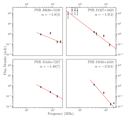
Figure 4: Flux density ($S_{\nu}$) measurements and best-fit power law spectra for PSRs J0636+5128, J1327+3423, J1434+7257, and J1816+4510. The triangle in the bottom-right plot represents an upper limit based on our lack of a detection of PSR J1816+4510 at 2 GHz.

We estimated uncertainties using standard error propagation, assuming uncertainties in $\Delta\nu$, $T_{\mathrm{sys}}$, and $\delta$ as follows. Day-to-day changes in $T_{\mathrm{sys}}$ on the level of a few K are expected, so we assumed $\sigma_{T_{\mathrm{sys}}}=5\,\mathrm{K}$. We assumed an uncertainty in $\delta$ equal to one phase bin, or $\sigma_{\delta}=1/128$, as they were chosen manually. Transient sources of RFI can alter the effective bandwidth of individual observations, so we assumed $\sigma_{\Delta\nu}=0.1\Delta\nu$. For pulsars with 350 MHz observations both before and after the aforementioned drastic change to the RFI environment which occurred in 2014, we increased $\sigma_{\Delta\nu}$ to 20 MHz to reflect the change.

As discussed earlier, PSR J0957$-$0619 was detected in the GBT 350 MHz Drift-scan survey. It was not detected in the GBNCC survey observation closest to its timing position, which was severely affected by RFI. In order to estimate $S_{\nu}$ at 350 MHz for this pulsar, and thus $\alpha$, we folded the discovery drift-scan observation on the pulsar ephemeris we obtained through our timing analysis. This yielded a 350 MHz profile which was weak, but sufficient to estimate $S_{\nu}$. The drift-scan observation was taken in the same setup as the GBNCC survey observations described in Section 2, but with only 50 MHz of bandwidth. The declination of the drifting telescope beam was $-06\arcdeg\,17\arcmin\,20\farcs 52$, sufficiently close to the true declination of the pulsar for the changing separation between the two not to significantly impact sensitivity during the 2.6-minute scan.

PSR J1816+4510 was not detected in three S-band observations with the GBT, $\sim$17 minutes total integration time. We place an upper limit at 2 GHz of $S_{\nu}<0.02$ mJy for this pulsar, assuming $\delta=0.06$ and $\mathrm{S/N}<6$.

We note that several pulsars in our sample have relatively flat spectra, with $\alpha$ even consistent with zero in a few cases. We selected each pulsar in the ATNF pulsar catalog (Manchester et al., 2005) with listed flux densities at both 400 and 1400 MHz (S400 and S1400) and calculated spectral indices using those measurements. Histograms comparing the distribution of spectral indices in ATNF versus those of the pulsars in this work are shown in Figure 5. We compared the two distributions using a statistical Kolmogorov–Smirnov test, and found that we could not refute the null hypothesis ($p\approx 0.5$) that the two samples are drawn from the same underlying distribution. This is perhaps contrary to the natural expectation that a low-frequency survey would discover a greater number of steeper-spectrum sources.

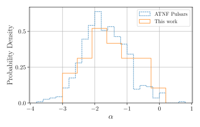
Figure 5: Histograms showing the distribution of pulsar spectral indices ($\alpha$) for pulsars in the ATNF catalog (dashed line) and those in this work (solid line). We calculated spectral indices for pulsars in the ATNF catalog using flux-density measurements at 400 and 1400 MHz. Visually, there appears to be an excess of flatter-spectrum pulsars in this work with $-1\lesssim\alpha\lesssim 0$, but a Kolmogorov–Smirnov test does not indicate that the two samples are drawn from different underlying distributions.

4 Pulsar Timing Analysis

For information about the discoveries and initial timing analysis of PSRs J0214+5222, J0636+5128, J1434+7257, and J1816+4510, see Stovall et al. (2014). When timing data first became available, each scan was processed using PRESTO, both to obtain an initial set of times of arrival (TOAs) and to note any changes in apparent spin periods due to possible Doppler shifting from binary motion. Only 350 and 820 MHz observations with the GBT were used for this purpose. We used rfifind to mask RFI and prepdata to produce timeseries at the pulsar’s known DM, which were searched with accelsearch for periodicity candidates with periods close to the discovery value. Finally, the raw data were folded with prepfold, which also searches for an improved spin period and period derivative.

Time-varying spin periods were noticed for PSRs J0032+6946 and J1239+3239, and preliminary sets of Keplerian parameters were obtained by performing a least-squares sinusoidal fit to the spin periods. These became the starting orbital parameters for these pulsars’ timing models.

We created standard profiles from the folded data using PRESTO’s pygaussfit.py to fit Gaussian components to the highest-S/N profile for each pulsar. If useful data were available at both 350 and 820 MHz, a separate standard profile was created at each frequency, and the two were aligned. We then cross-correlated these standard profiles in the Fourier domain with the folded data (Taylor, 1992) using get_TOAs.py to obtain TOAs. We created three TOAs per 5 – 15 minute observation to allow fitting for spin frequency at each epoch, enabling phase connection across day–week-long timespans at first, and eventually across each pulsar’s entire data set. These initial phase-connected timing solutions were obtained separately by several of the authors, who used either the tempo or tempo2 timing software.

Henceforth, we discuss the data processing in the context of a single pulsar’s set of timing observations. Raw data were folded on the new pulsar ephemeris, using fold_psrfits to fold search-mode data on the pulsar’s spin period, resulting in 10 s sub-integrations. psrchive , a suite of pulsar data analysis software, was used for all further data processing. Any data containing polarization information were first reduced to total intensities. RFI was excised automatically using paz both before and after averaging, or “scrunching”, to 128 frequency channels, in order to zap RFI from both single frequency channels and larger portions of the band as thoroughly as possible without removing useful data. Then, each frequency-scrunched observation was examined by eye and any remaining RFI was removed with pazi. Where applicable, any periods of nulling at the beginning or end of an observation were removed by extracting the appropriate sub-integrations using pam.

We then used psradd to phase-align observations and sum them to create an average profile for each band. To each of these, we used paas to fit Gaussian components, resulting in noise-free template profiles. Each observation was then scrunched in time and frequency to achieve the desired number of sub-integrations and subbands. These numbers were generally 2 – 5, with the exact number of each being chosen to both enable a determination of DM and avoid degrading S/N below 6. We set the maximum sub-integration length for PSR J0636+5128 at 2.5% of its 1.6 hr orbital period, to minimize any smearing within sub-integrations due to Doppler shifts caused by orbital motion. Two full-orbit observations of PSR J1816+4510 were split into many 9 – 10 minute sub-integrations. Once a timing solution was initially reached, lower-S/N observations were sometimes fully scrunched in time so that more subbands could be used, in order to better constrain DM.

Data from AO observations of PSR J1327+3423 were reduced according to the usual NANOGrav procedure described in NANOGrav Collaboration et al. (2015), from RFI removal and flux and polarization calibration, to time- and frequency-scrunching to sub-integrations up to 30 minutes long, with 64 subbands. From that point, we followed the steps laid out above for the creation of template profiles. For consistency with the AO data, we fully time-scrunched our 820 MHz GBT observations of this pulsar and divided them into 32 subbands.

After scrunching, and ensuring standard profiles were correctly aligned (see below), one TOA per subband for each sub-integration was calculated using pat. TOAs were later excised from the timing analysis if they were outliers, due to either very large uncertainty or corresponding timing residual $\delta t=\mathrm{TOA_{meas}}-\mathrm{TOA_{pred}}$, where $\mathrm{TOA_{meas}}$ is the measured TOA and $\mathrm{TOA_{pred}}$ is the corresponding TOA predicted by the pulsar’s timing model. 316 out of 8726 total TOAs were flagged as outliers in this manner.

We eliminated undesired offsets between TOAs from different telescopes/receivers using three methods. First, the template profiles were aligned to the same reference phase using pas. Second, for TOAs obtained using the GUPPI or VEGAS backends, known timing offsets were removed by adding TIME flags to TOA (tim) files. Timing offsets between different observing modes and receivers at the GBT were determined using guppi_offsets for GUPPI observations: e.g. search-mode 350 MHz data is offset from fold-mode 820 MHz data by 78.08 $\mu$s; and vpmTimingOffsets.py (a command on GBO computers) for VEGAS. Third, for pulsars with observations at different telescopes, timing offsets between different observatories and receivers were fit for using JUMPs (an arbitrary phase offset, which is fit in the timing model) in the pulsar parameter (par) files. Due to missing data files, we were unable to reproduce TOAs corresponding to some older observations of PSRs J0214+5222 and J1816+4510, and instead used the same TOAs which were used in Stovall et al. (2014). In order to account for the different folding ephemerides and standard profiles used to generate these old TOAs, we also fit JUMPs for these older TOAs, doing so separately for, e.g., 350 and 820 MHz.

Timing parameters were then fit for iteratively using tempo2, using the DE440 solar system ephemeris and TT(BIPM2021) time standard. The introduction of new timing parameters, such as proper motion and parallax, was tested during this process. If it was not obvious whether a new parameter was significant, we used a statistical $F$-test to compare the $\chi^{2}$ of the fit with and without the new parameter, only including it in the timing model if it passed 3-$\sigma$ confidence with $\alpha<0.0027$. After a timing solution was reached, the data were refolded using the updated ephemeris, TOAs were re-created using the same method as before, and timing parameters were fit once again using this final set of TOAs. This last step was necessary because the pulsar ephemeris originally used to fold the data was necessarily incorrect, and this could introduce errors into the final timing solution.

4.1 Timing of Binary Pulsars

Pulsar binary orbits are characterized by, at minimum, five Keplerian parameters: the orbital period $P_{\mathrm{b}}$, projected semimajor axis $x=a\sin i/c$ (where $a$ is the semimajor axis and $i$ is the inclination of the orbit, $i=90\arcdeg$ being edge-on when viewed from Earth), eccentricity $e$, longitude of periastron $\omega$, and time of periastron $T_{0}$. For low-eccentricity orbits, there are high covariances between $\omega$ and $T_{0}$, resulting in high uncertainties (Lange et al., 2001). All of the binary pulsars in this work have eccentricities which are low enough to cause these high covariances.

Therefore, we used the Lange et al. (2001, ELL1) binary model, which uses an approximation for the Roemer delay ($\Delta_{\mathrm{R}}$) and parameterizes the orbit in terms of the time of ascending node,

$$T_{\mathrm{asc}}=T_{0}-P_{\mathrm{b}}(\omega/2\pi),$$ (2)

and the Laplace-Lagrange parameters,

$$e_{1}=e\sin\omega\ \ \mathrm{and}\ \ e_{2}=e\cos\omega.$$ (3)

tempo2’s implementation of the ELL1 model contains terms for $\Delta_{\mathrm{R}}$ up to first order in $e$. This is sufficient for pulsars with $\delta t_{\mathrm{RMS}}/N_{\mathrm{TOA}}^{1/2}\gtrsim xe^{2}$, but PSRs J0032+6946 and J0214+5222 do not satisfy this requirement. We attempted to use the Blandford & Teukolsky (1976) model for these pulsars, which uses $e$, $T_{0}$, $\omega$, and the full expression for $\Delta_{\mathrm{R}}$. The timing solutions seemed serviceable, but covariances between $T_{0}$ and $\omega$ were quite high.

Fortunately, the second-order terms for $\Delta_{\mathrm{R}}$, calculated by Zhu et al. (2019), have been implemented in (current version, not the latest release of) the pulsar timing software PINT (Luo et al., 2021). These are sufficient for PSR J0032+6946, but PSR J0214+5222 has $xe^{3}>\delta t_{\mathrm{RMS}}/N_{\mathrm{TOA}}^{1/2}$. Therefore, to reach an accurate solution for this pulsar’s binary motion, it is necessary to extend the approximation for the Roemer delay to third order in $e$:

$$\Delta_{\mathrm{R}}\simeq\ x\bigg{(}\sin\phi+\frac{e_{2}}{2}\sin 2\phi-\frac{e_{1}}{2}\cos 2\phi\bigg{)}-\frac{x}{8}\Big{(}5e_{2}^{2}\sin\phi-3e_{2}^{2}\sin 3\phi-2e_{1}e_{2}\cos\phi+6e_{1}e_{2}\cos 3\phi+3e_{1}^{2}\sin\phi+3e_{1}^{2}\sin 3\phi\Big{)}$$

$$-\frac{x}{12}\Big{(}5e_{2}^{3}\sin 2\phi+3e_{1}^{2}e_{2}\sin 2\phi-6e_{1}e_{2}^{2}\cos 2\phi-4e_{1}^{3}\cos 2\phi-4e_{2}^{3}\sin 4\phi+12e_{1}^{2}e_{2}\sin 4\phi+12e_{1}e_{2}^{2}\cos 4\phi-4e_{1}^{3}\cos 4\phi\Big{)}$$ (4)

(note that we have corrected here an index swap in the first-order terms present in Equation 1 of Zhu et al. (2019)), where $\phi$ is the orbital phase used in the ELL1 model, written in radians as

$$\phi(t)=(t-T_{\mathrm{asc}})(2\pi/P_{\mathrm{b}}).$$ (5)

This expression is sufficient for PSR J0214+5222, since $xe^{4}\simeq 0.14$ $\mu$s. We implemented this expression in PINT, which we used to produce final timing solutions for these two pulsars. Note that we did not use this “third-order ELL1” model for PSRs J0636+5128, J1239+3239, or J1816+4510; the first-order ELL1 model in tempo2 is sufficient for these systems.

4.2 Accounting for DM Variations

Variations in DM are expected to occur on $\sim$monthly timescales due to the line of sight to the pulsar traversing regions with different electron densities. These effects are on the order of $10^{-(3-4)}$ pc cm^-3 (Jones et al., 2017), significantly lower than the precision of some of our DM measurements. One method of modeling variations in DM in the timing model is fitting a piecewise constant function called DMX. A fixed reference value for DM is chosen, and each DMX parameter describes an offset from that value at a particular epoch (a grouping of observations, usually 1 – 7 days in length).

For most of our pulsars, applying the DMX model is unnecessary, so we simply note that any reported DM uncertainties $\lesssim 0.001$ pc cm^-3 are likely underestimated. However, DM variations could lead to a meaningful signature in the residuals for our most precisely-timed pulsars. The dispersion delay between two frequencies $\nu_{1}$ and $\nu_{2}$ (in MHz) is given by

$$\Delta t\simeq 4.15\times 10^{6}\,\mathrm{ms}\times(\nu_{1}^{-2}-\nu_{2}^{-2})\times\mathrm{DM}$$ (6)

(Lorimer & Kramer, 2004). For a change $\sim 10^{-3}$ pc cm^-3, the corresponding delay compared to infinite frequency at 820 MHz is $\sim$ 6.2 $\mu$s, comparable to $\delta t_{\mathrm{RMS}}$ for our three most precisely-timed pulsars—J0636+5128, J1327+3423, and J1816+4510—which have $\delta t_{\mathrm{RMS}}<10$ $\mu$s. Also, without fitting for DMX, the timing fit for PSR J1816+4510 was somewhat poor, reduced $\chi^{2}\sim 3$. Several additional parameters, such as $\ddot{\nu}$, $\dot{\nu}_{\mathrm{b}}$, $\dot{x}$, $\dot{e}_{1}$, and $\dot{e}_{2}$, appeared to be marginally significant, but their inclusion did not greatly improve $\chi_{\mathrm{red}}^{2}$. PSRs J0636+5128 and J1327+3423 also had $\chi_{\mathrm{red}}^{2}\sim 2$ before DMX was introduced.

We split the observations of these pulsars into 6.5-day epochs and fit for one DMX parameter per epoch. We disabled the solar wind model in tempo2 by setting the solar wind density at 1 AU distance from the Sun to zero, so that all DM variations were modeled by DMX, including those due to the solar wind. Certain observations of PSR J1816+4510 presented in Stovall et al. (2014) have only single-frequency TOAs. In some cases, the corresponding raw data are now missing, meaning we could not re-create the TOAs with retained frequency information. For epochs containing only such TOAs, we fixed the value of the piecewise constant DMX function to zero. In each case, the fit was improved after adding DMX, and additional orbital parameters were rendered insignificant for PSR J1816+4510.

5 Results

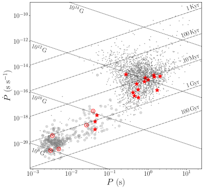
Figure 6: The pulsars presented in this work are plotted as red stars (or as dots surrounded by circles, if in binary systems) on this $P$–$\dot{P}$ diagram, with values for the rest taken from the ATNF pulsar catalog. Lines of constant minimum surface magnetic field $B_{\mathrm{surf}}$ (in Gauss; dashed lines) and characteristic age $\tau_{\mathrm{c}}$ (dotted-dashed lines) are also shown.

Each pulsar’s spin frequency $\nu$ and frequency derivative $\dot{\nu}$ are given in Table 4 along with general information about each timing solution. We estimated distances to each of the pulsars based on their DMs, using the NE2001 (Cordes & Lazio, 2002, 2003) and YMW16 (Yao et al., 2017) Galactic free electron density models, reporting the distances given by each model. These are reported, along with positions in Right Ascension (R.A.) and Declination (decl.) and in Galactic coordinates, in Table 5. Derived quantities are listed in Table 6. We show a $P$–$\dot{P}$ diagram of our pulsars, as well as all pulsars in the ATNF pulsar catalog (Manchester et al., 2005), in Figure 6.

Table 4: Rotational and Timing Parameters of GBNCC Pulsars

PSR	$\nu$	$\dot{\nu}$	Epoch	Data Span	$\delta t_{\mathrm{RMS}}$	$N_{\mathrm{TOA}}$	EFAC
	(Hz)	(Hz s-1)	(MJD)	(MJD)	($\mu$s)
J0032+6946	27.171119572492(3)	$-$2.65006(3)$\times$10-15	56736	55169–58303	0019.1	1430	1.08
J0141+6303	21.42232445491(4)	$-$7.65(2)$\times$10-16	57431	57072–57789	0075.1	0122	1.03
J0214+5222	40.691271761863(5)	$-$4.9002(7)$\times$10-16	56974	55353–58594	0077.8	0951	1.05
J0415+6111	002.27174933348(6)	$-$2.8(4)$\times$10-16	57234	57071–57397	0609.4	0038	1.04
J0636+5128	348.55923172059(1)	$-$4.262(8)$\times$10-16	56712	56027–57397	0001.9	1403	1.17
J0957$-$0619	000.58014346794(2)	$-$5(1)$\times$10-17	57220	57071–57369	0767.0	0067	1.07
J1239+3239	212.71645129924(2)	$-$1.752(5)$\times$10-16	57733	56054–59412	0021.5	0283	1.13
J1327+3423	24.089008071282(2)	$-$7.514(3)$\times$10-17	58067	57079–59055	0002.7	1575	1.18
J1434+7257	23.957175372381(1)	$-$3.1476(4)$\times$10-16	56731	55196–58266	0031.4	0351	1.11
J1505$-$2524	001.000750227637(9)	$-$9.812(6)$\times$10-16	57077	56754–57399	0384.0	0588	1.13
J1530$-$2114	001.97887013684(2)	$-$1.817(1)$\times$10-15	56994	56588–57399	0443.1	0062	1.04
J1816+4510	313.17493532200(3)	$-$4.2246(5)$\times$10-15	56945	55508–58382	0008.2	0749	1.45
J1913+3732	001.174979047088(6)	$-$1.9021(2)$\times$10-15	56694	55988–57399	0373.5	0189	1.04
J1929+6630	001.24066854069(5)	$-$1.079(6)$\times$10-15	57136	56872–57399	0289.2	0031	0.96
J1930+6205	000.68675905720(8)	$-$7.85(5)$\times$10-16	57027	56655–57399	0828.6	0033	0.97
J2104+2830	002.46469868711(3)	$-$5.930(9)$\times$10-16	56743	56089–57397	0293.6	0072	0.99
J2115+6702	001.81119402046(5)	$-$5.5(4)$\times$10-16	57235	57072–57397	0693.7	0038	0.99
J2145+2158	000.70472549203(2)	$-$1.105(2)$\times$10-15	56928	56459–57397	1725.7	0060	1.48
J2210+5712	000.48705587420(1)	$-$4.4(1)$\times$10-16	57236	57072–57399	0953.0	0074	1.11
J2326+6243	003.75729497728(2)	$-$3.617(1)$\times$10-14	57234	57072–57397	0336.9	0216	1.02
J2354$-$2250	001.792046218541(1)	$-$1.287(1)$\times$10-16	58207	56666–59748	0286.1	0078	1.08

Note. — For each pulsar in this analysis, measurements of spin frequency $\nu$ (at the listed reference epoch) and its derivative $\dot{\nu}$ are listed, with the $1$-$\sigma$ uncertainties on the last digit in parentheses. Also listed are the dates spanned by the TOAs, timing residual rms $\delta t_{\mathrm{RMS}}$, number of TOAs $N_{\mathrm{TOA}}$, and EFAC, a scaling factor applied to TOA uncertainties which forces the reduced $\chi^{2}$ to equal unity. All timing models use the DE440 solar system ephemeris and are referenced to the TT(BIPM2021) time standard.

Table 5: Coordinates and DMs of GBNCC Pulsars

PSR	Measured			Derived
	$\alpha_{\mathrm{J2000}}$	$\delta_{\mathrm{J2000}}$	DM	$\ell$	$b$	D${}^{\mathrm{NE2001}}_{\mathrm{DM}}$	D${}^{\mathrm{YMW16}}_{\mathrm{DM}}$
			(pc cm-3)	($\arcdeg$)	($\arcdeg$)	(kpc)	(kpc)
J0032+6946	$00^{\rm h}\,32^{\rm m}\,41\,\fs 2477(3)$	$+69\arcdeg\,46\arcmin\,28\,\farcs 047(2)$	79.9988(2)	121.30	6.96	02.8	02.3
J0214+5222	$02^{\rm h}\,14^{\rm m}\,55\,\fs 2746(2)$	$+52\arcdeg\,22\arcmin\,40\,\farcs 907(3)$	22.0371(3)	135.63	$-$8.42	01.0	01.2
J0141+6303	$01^{\rm h}\,41^{\rm m}\,45\,\fs 761(1)$	$+63\arcdeg\,03\arcmin\,49\,\farcs 445(9)$	272.762(2)00	128.60	0.75	44.3	08.8
J0415+6111	$04^{\rm h}\,15^{\rm m}\,51\,\fs 63(5)$	$+61\arcdeg\,11\arcmin\,51\,\farcs 8(3)$	70.8(1)000	145.15	7.49	02.3	01.8
J0636+5128	$06^{\rm h}\,36^{\rm m}\,04\,\fs 84705(3)$	$+51\arcdeg\,28\arcmin\,59\,\farcs 9658(6)$	string11.1075string	163.91	18.64	00.5	00.2
J0957$-$0619	$09^{\rm h}\,57^{\rm m}\,08\,\fs 12(2)$	$-06\arcdeg\,19\arcmin\,37\,\farcs 5(9)$	27.3(1)000	244.83	36.20	01.2	02.5
J1239+3239	$12^{\rm h}\,39^{\rm m}\,27\,\fs 3140(1)$	$+32\arcdeg\,39\arcmin\,23\,\farcs 379(2)$	16.8590(1)	147.36	83.89	01.5	02.2
J1327+3423	$13^{\rm h}\,27^{\rm m}\,07\,\fs 54861(3)$	$+34\arcdeg\,23\arcmin\,37\,\farcs 6777(8)$	0string4.1829string	78.61	79.45	00.5	00.3
J1434+7257	$14^{\rm h}\,33^{\rm m}\,59\,\fs 7338(4)$	$+72\arcdeg\,57\arcmin\,26\,\farcs 495(1)$	12.6118(1)	113.08	42.15	00.7	01.0
J1505$-$2524	$15^{\rm h}\,05^{\rm m}\,22\,\fs 529(3)$	$-25\arcdeg\,24\arcmin\,50\,\farcs 1(1)$	44.79(2)00	337.42	28.34	01.9	03.9
J1530$-$2114	$15^{\rm h}\,30^{\rm m}\,43\,\fs 00(4)$	$-21\arcdeg\,14\arcmin\,21(2)\arcsec$	37.95(1)00	345.54	28.16	01.6	02.6
J1816+4510	$18^{\rm h}\,16^{\rm m}\,35\,\fs 9346(3)$	$+45\arcdeg\,10\arcmin\,33\,\farcs 855(3)$	string38.8881string	72.83	24.74	02.4	04.4
J1913+3732	$19^{\rm h}\,13^{\rm m}\,27\,\fs 892(3)$	$+37\arcdeg\,32\arcmin\,12\,\farcs 35(3)$	72.29(2)00	69.10	12.13	04.2	07.6
J1929+6630	$19^{\rm h}\,29^{\rm m}\,07\,\fs 22(1)$	$+66\arcdeg\,30\arcmin\,56\,\farcs 0(1)$	59.74(8)00	98.01	21.11	04.3	08.2
J1930+6205	$19^{\rm h}\,30^{\rm m}\,42\,\fs 45(3)$	$+62\arcdeg\,05\arcmin\,31\,\farcs 7(2)$	67.5(3)000	93.66	19.39	05.7	10.7
J2104+2830	$21^{\rm h}\,04^{\rm m}\,24\,\fs 133(3)$	$+28\arcdeg\,30\arcmin\,57\,\farcs 58(4)$	62.16(5)00	74.18	$-$12.18	03.7	05.7
J2115+6702	$21^{\rm h}\,15^{\rm m}\,00\,\fs 42(2)$	$+67\arcdeg\,02\arcmin\,31\,\farcs 8(4)$	.string54.5(1.3)00	104.05	12.49	02.7	02.9
J2145+2158	$21^{\rm h}\,45^{\rm m}\,04\,\fs 24(2)$	$+21\arcdeg\,58\arcmin\,10\,\farcs 9(3)$	44.3(1)000	75.72	$-$23.37	02.8	05.4
J2210+5712	$22^{\rm h}\,10^{\rm m}\,08\,\fs 27(2)$	$+57\arcdeg\,12\arcmin\,59\,\farcs 8(4)$	192.9(2)0000	102.42	0.91	06.2	03.9
J2326+6243	$23^{\rm h}\,26^{\rm m}\,41\,\fs 492(7)$	$+62\arcdeg\,43\arcmin\,22\,\farcs 49(7)$	193.61(3)000	113.40	1.43	08.5	04.4
J2354$-$2250	$23^{\rm h}\,54^{\rm m}\,17\,\fs 688(3)$	$-22\arcdeg\,50\arcmin\,05\,\farcs 6(1)$	10.00(1)00	48.15	$-$76.37	00.4	01.1

Note. — We report pulsar positions in Right Ascension and Declination referenced to the J2000 epoch ($\alpha_{\mathrm{J2000}}$ and $\delta_{\mathrm{J2000}}$, respectively), and dispersion measures (DMs) for each pulsar in this analysis. Values in parentheses are the $1$-$\sigma$ uncertainty in the last digit. We also present a set of parameters derived from measured positions and DMs: Galactic longitude $\ell$ and latitude $b$, and DM-derived distances D_DM using the NE2001 (Cordes & Lazio, 2002) and YMW16 (Yao et al., 2017) Galactic electron density models, as indicated. These distance estimates should be taken to have large fractional uncertainties, $\sim$30 – 50% (Deller et al., 2019). In some cases, the reported precision in DM goes beyond expected month$-$year-timescale variability. We account for these changes using a DMX model (see Section 4.2 and Figure 11) for PSRs J0636+5128, J1327+3423, and J1816+4510, and list here the reference DM used in that model. This treatment was not necessary for the other pulsars with such listed precision, so we simply note that the uncertainties listed for DMs are likely underestimated if they are $\lesssim$0.001 pc cm^-3.

Table 6: Derived Common Properties of GBNCC Pulsars

PSR	$P$	$\dot{P}$	$\tau_{\mathrm{c}}$	$B_{\mathrm{surf}}$	$\dot{E}$
	(s)	(s s-1)	(yr)	(Gauss)	(erg s-1)
J0032+6946	0.036803783419083(3)	3.58955(4)$\times$10-18	1.6$\times$108	1.2$\times$1010	2.8$\times$1033
J0214+5222	0.024575294816350(3)	2.9594(4)$\times$10-19	1.3$\times$109	2.7$\times$109	7.9$\times$1032
J0214+5222	0.024575294816349(3)	2.9596(4)$\times$10-19	1.3$\times$109	2.7$\times$109	7.9$\times$1032
J0415+6111	0.44018941054(1)	5.5(8)$\times$10-17	1.3$\times$108	1.6$\times$1011	2.5$\times$1031
J0636+5128	0.00286895284644653(9)	3.508(7)$\times$10-21	1.3$\times$1010	1.0$\times$108	5.9$\times$1033
J0957$-$0619	1.72371155631(5)	1.5(3)$\times$10-16	1.8$\times$108	5.1$\times$1011	1.2$\times$1030
J1239+3239	0.0047010938453146(4)	3.87(1)$\times$10-21	1.9$\times$1010	1.4$\times$108	1.5$\times$1033
J1327+3423	0.041512709740513(3)	1.2948(5)$\times$10-19	5.1$\times$109	2.3$\times$109	7.1$\times$1031
J1434+7257	0.041741147879765(2)	5.4841(6)$\times$10-19	1.2$\times$109	4.8$\times$109	3.0$\times$1032
J1505$-$2524	0.999250334782(9)	9.798(6)$\times$10-16	1.6$\times$107	1.0$\times$1012	3.9$\times$1031
J1530$-$2114	0.505338870593(4)	4.640(3)$\times$10-16	1.7$\times$107	4.9$\times$1011	1.4$\times$1032
J1816+4510	0.0031931035571918(3)	4.3073(5)$\times$10-20	1.2$\times$109	3.8$\times$108	5.2$\times$1034
J1913+3732	0.851079006454(4)	1.3778(1)$\times$10-15	9.8$\times$106	1.1$\times$1012	8.8$\times$1031
J1929+6630	0.80601705226(3)	7.01(4)$\times$10-16	1.8$\times$107	7.6$\times$1011	5.3$\times$1031
J1930+6205	1.4561147604(2)	1.66(1)$\times$10-15	1.4$\times$107	1.6$\times$1012	2.1$\times$1031
J2104+2830	0.405729108077(5)	9.76(1)$\times$10-17	6.6$\times$107	2.0$\times$1011	5.8$\times$1031
J2115+6702	0.55212196413(2)	1.7(1)$\times$10-16	5.3$\times$107	3.1$\times$1011	3.9$\times$1031
J2145+2158	1.41899223358(5)	2.226(4)$\times$10-15	1.0$\times$107	1.8$\times$1012	3.1$\times$1031
J2210+5712	2.05315252924(6)	1.84(4)$\times$10-15	1.8$\times$107	2.0$\times$1012	8.4$\times$1030
J2326+6243	0.266148919913(2)	2.562(1)$\times$10-15	1.6$\times$106	8.4$\times$1011	5.4$\times$1033
J2354$-$2250	0.5580213220250(4)	4.008(3)$\times$10-17	2.2$\times$108	1.5$\times$1011	9.1$\times$1030

Note. — We report properties derived from directly-measured quantities for each pulsar in this analysis: spin periods $P$, period derivatives $\dot{P}$, characteristic ages $\tau_{\mathrm{c}}$, inferred surface magnetic fields $B_{\mathrm{surf}}$, and spindown luminosities $\dot{E}$. These have not been corrected for apparent acceleration caused by kinematic effects. We calculate $\dot{E}$ and $B_{\mathrm{surf}}$ assuming a moment of inertia $I=10^{45}$ g cm²; additionally, $B_{\mathrm{surf}}$ assumes a neutron star radius $R=10$ km and $\alpha=90^{\circ}$ (angle between spin/magnetic axes). Calculating $\tau_{\mathrm{c}}$ relies on the assumption that spin-down is fully due to magnetic dipole radiation (braking index $n=3$) and that the initial spin period is negligible. Values in parentheses are the $1$-$\sigma$ uncertainty in the last digit.

Figures 7, 8, 9, and 10 show each pulsar’s final set of timing residuals. DMX timeseries are shown in Figure 11. PSRs J0032+6946, J0214+5222, J0636+5128, J1239+3239, and J1816+4510 are in binary systems. Timing residuals for these pulsars are plotted against orbital phase in Figure 12, and we list pulsars’ best-fit orbital parameters in Table 7.

Table 7: Orbital Parameters for GBNCC Pulsars in Binary Systems

Quantity		PSR J0032+6946	PSR J0214+5222	PSR J0636+5128	PSR J1239+3239	PSR J1816+4510
Measured
$\nu_{\mathrm{b}}$	(Hz)	2.193632768(6)$\times 10^{-8}$	2.260385778(9)$\times 10^{-8}$	0.0001739119636(3)	2.833032117(4)$\times 10^{-6}$	3.2070609894(7)$\times 10^{-5}$
$a\sin i/c$	(s)	178.674768(3)	174.565762(5)	0.0089858(1)	2.371127(2)	0.5954006(6)
$T_{\mathrm{asc}}$	(MJD)	56399.134959(4)	56339.115121(4)	56711.9950666(4)	57730.0800015(9)	56945.0911546(2)
$e\sin\omega$		string0.00028554(2)	$-$0.00271145(5)	string1(2)$\times 10^{-5}$	5(2)$\times 10^{-6}$	string8(2)$\times 10^{-6}$
$e\cos\omega$		$-$0.00044865(3)	$-$0.00458640(6)	$-$1(2)$\times 10^{-5}$	0(2)$\times 10^{-6}$	$-$1(2)$\times 10^{-6}$
$\dot{\nu}_{\mathrm{b}}$	(Hz s-1)	…	…	$-$7.1(7)$\times 10^{-20}$	…	…
$\ddot{\nu}_{\mathrm{b}}$	(Hz s-2)	…	…	$-$2.4(8)$\times 10^{-27}$	…	…
$\dot{x}$	(s s-1)	…	$-$2.1(6)$\times 10^{-13}$	…	…	…
Derived
$P_{\mathrm{b}}$	(days)	527.621316(2)	512.039767(2)	0.0665513392(1)	4.085401647(6)	0.36089348198(8)
$T_{0}$	(MJD)	56615.350(3)	56638.6460(8)	56712.02(2)	57731.1(3)	56945.19(1)
$\omega$	(°)	147.525(2)	210.5913(6)	145(106)	89(22)	97(14)
$e$		0.00053181(3)	0.00532795(5)	1(2)$\times 10^{-5}$	5(2)$\times 10^{-6}$	8(2)$\times 10^{-6}$
$f_{\mathrm{M}}$	(M☉)	2.20$\times 10^{-2}$	2.18$\times 10^{-2}$	1.76$\times 10^{-7}$	8.58$\times 10^{-4}$	1.74$\times 10^{-3}$
$M_{\mathrm{c}}$	(M☉)	0.417	0.416	0.007	0.126	0.162

Note. — We report binary parameters for each pulsar in this analysis with evidence of a binary companion. These include measured orbital frequencies $\nu_{\mathrm{b}}$, semimajor axes projected along the line of sight $x=a\sin{i}/c$, times of ascending node $T_{\mathrm{asc}}$, and first and second Laplace-Lagrange parameters, $e_{1}=e\sin\omega$ and $e_{2}=e\cos\omega$. For certain pulsars, we also report first and second derivatives of orbital frequency ($\dot{\nu}_{\mathrm{b}}$ and $\ddot{\nu}_{\mathrm{b}}$, respectively), and a time derivative of the projected semimajor axis, $\dot{x}$. Using the measured binary parameters, we derive the orbital period $P_{\mathrm{b}}$, time of periastron $T_{0}$, longitude of periastron $\omega$, eccentricity $e$, the binary mass function $f_{\mathrm{M}}=(M_{\mathrm{c}}\sin i)^{3}(M_{\mathrm{p}}+M_{\mathrm{c}})^{-2}$, and the minimum companion mass $M_{\mathrm{c,min}}=f_{\mathrm{M}}(M_{\mathrm{p}}=1.4\,\mathrm{M}_{\sun},i=90\arcdeg)$. We used the ELL1 binary model for each pulsar, but with two different implementations: for PSRs J0032+6946 and J0214+5222, we implemented Equation 4, which expresses the Roemer delay up to third order in $e$, in PINT; for the other pulsars, we used the ELL1 binary model as implemented in tempo2, which only includes the first-order Roemer-delay terms. Values in parentheses are the $1$-$\sigma$ uncertainty in the last digit.

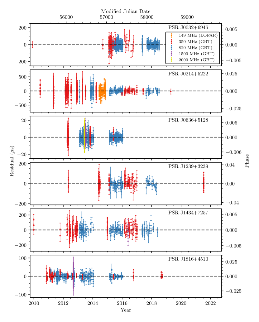
Figure 7: Timing residuals for six of the pulsars in this analysis. Residuals at 149 MHz from LOFAR observations are plotted in orange, while 350, 820, 1500, and 2000 MHz residuals from GBT observations are plotted in red, blue, purple, and yellow, respectively. The dashed gray lines correspond to a residual of zero. Error bars are the 1-$\sigma$ uncertainties in each TOA.

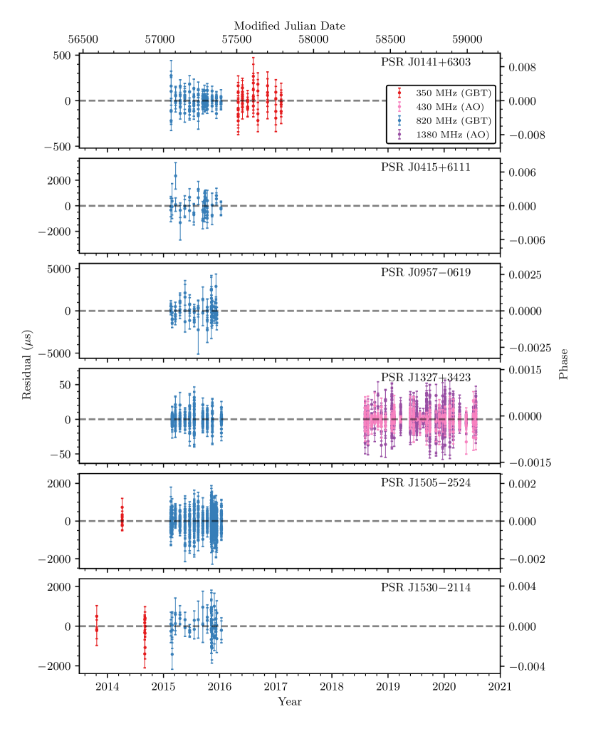
Figure 8: Timing residuals for six pulsars, with 430 and 1380 MHz residuals from NANOGrav AO observations plotted in pink and purple, respectively, and 350 and 820 MHz residuals from GBT observations plotted in red and blue, respectively. The dashed gray lines correspond to a residual of zero. Error bars are the 1-$\sigma$ uncertainties in each TOA.

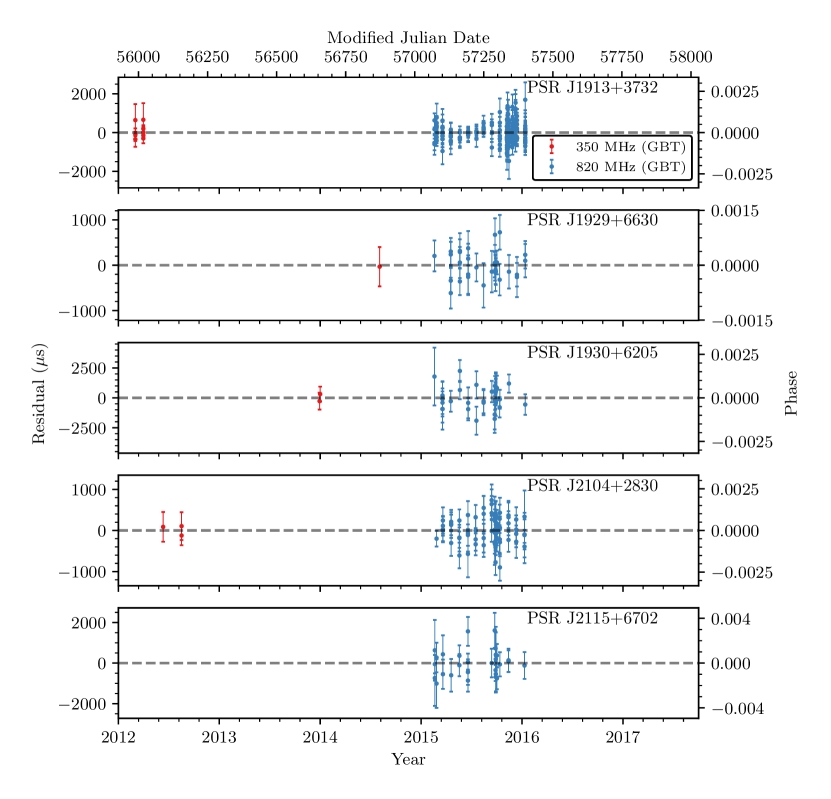
Figure 9: Timing residuals for five pulsars, with 350 and 820 MHz residuals from GBT observations plotted in red and blue, respectively. The dashed gray lines correspond to a residual of zero. Error bars are the 1-$\sigma$ uncertainties in each TOA.

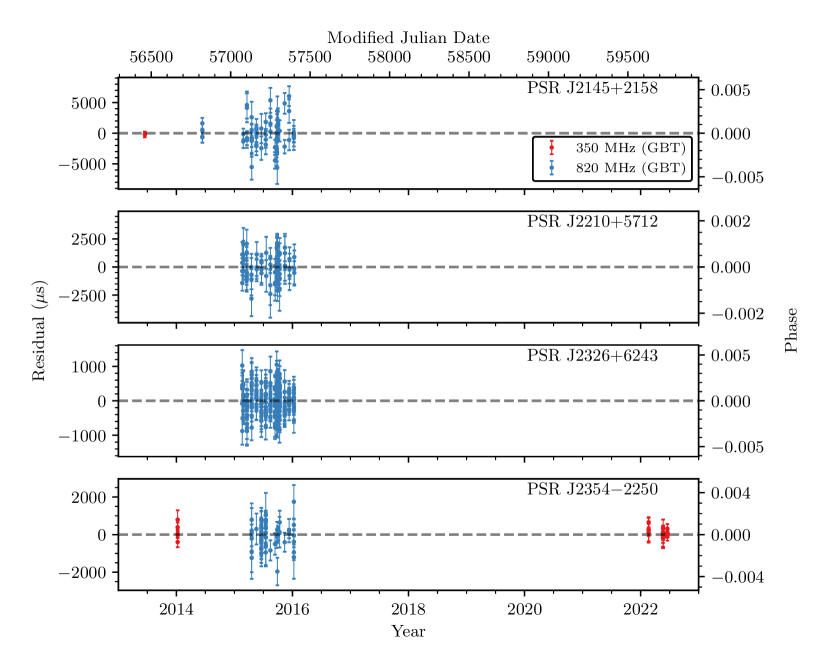
Figure 10: Timing residuals for the final four pulsars, with 350 and 820 MHz residuals from GBT observations plotted in red and blue, respectively. The dashed gray lines correspond to a residual of zero. Error bars are the 1-$\sigma$ uncertainties in each TOA.

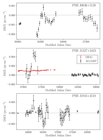
Figure 11: DMX timeseries for PSRs J0636+5128, J1327+3423, and J1816+4510, showing the offset from a fiducial DM value at each epoch. The dashed gray line in each plot corresponds to an offset of zero. The plot for PSR J1327+3423 shows DMX in red corresponding to LWA1 observations; the points in black are from the GBT (before MJD 58000) and AO (after MJD 58000). Epochs for which we were unable to fit for DMX (described in Section 4.2) are not shown. Error bars correspond to the 1-$\sigma$ uncertainty in DMX reported by tempo2.

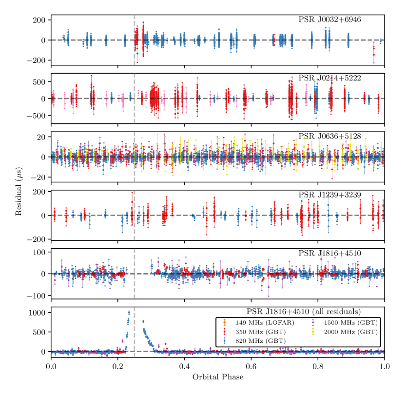
Figure 12: Timing residuals for the five pulsars in binary systems are plotted vs. orbital phase (see Equation 5, but one orbit = 1.0 instead of $2\pi$ radians). The gray dashed vertical line at $\phi=0.25$ denotes superior conjunction, and the horizontal dashed lines correspond to a residual of zero. The second set of residuals from the bottom are the residuals for PSR J1816+4510 which contributed to our timing solution. The bottom-most set of residuals are all of our residuals for PSR J1816+4510, including those which exhibit additional timing delays before and after eclipse. In the latter set, TOAs from the full-orbit observations of PSR J1816+4510 were created with shorter sub-integrations so that the behavior near eclipse can be seen more easily. The 350, 820, 1500, and 2000 MHz residuals from GBT observations are plotted in red, blue, purple, and yellow, respectively. Error bars are the 1-$\sigma$ uncertainties in each TOA.

We measured proper motions in R.A. ($\mu_{\alpha}=\dot{\alpha}\cos\delta$, where $\alpha=\mathrm{R.A.}$ and $\delta=\mathrm{decl.}$) and decl. ($\mu_{\delta}=\dot{\delta}$) for five pulsars with several years of timing data: PSRs J0214+5222 (only $\mu_{\alpha}$ is significant), J0636+5128, J1327+3423, J1434+7257, and J1816+4510. Using total proper motions and DM-derived distances, we calculated transverse velocities $v_{t}$ for these pulsars. This allows the determination of the apparent rate of spindown due to the relative transverse motion between the pulsar and solar system barycenter, known as the Shklovskii effect (Shklovskii, 1970), which we write as $\dot{P}_{\mathrm{S}}$. Using the same method laid out in Swiggum et al. (2023), based on Guo et al. (2021), we also calculate a correction $\dot{P}_{\mathrm{G}}$ due to the pulsar’s acceleration in the Galactic potential, using the most recent value for the distance between the Sun and the Galactic center, $R_{0}=8.275(34)$ kpc (Holmberg & Flynn, 2004), and for the circular velocity of the Sun around the Galactic center, $\Phi_{0}=240.5(4.1)$ km s^-1 (GRAVITY Collaboration et al., 2021).

Together, these corrections give us each pulsar’s intrinsic rate of spindown, $\dot{P}_{\mathrm{int}}=\dot{P}-\dot{P}_{\mathrm{S}}-\dot{P}_{\mathrm{G}}$, which we then use to re-calculate other derived parameters which depend on $\dot{P}$. We list these corrected quantities, along with proper motions and transverse velocities, in Table 8. Each pulsar has two sets of calculated velocities and corrections, each assuming either the NE2001 or YMW16 DM distance.

Table 8: Proper Motions and Kinematic Corrections for Five GBNCC Pulsars

PSR	$\mu_{\alpha}$	$\mu_{\delta}$	$D_{\mathrm{DM}}$	$v_{\mathrm{t}}$	$\dot{P}_{\mathrm{G}}$	$\dot{P}_{\mathrm{S}}$	$\dot{P}_{\mathrm{int}}$	$B_{\mathrm{surf}}$	$\tau_{\mathrm{c}}$	$\dot{E}$
	(mas yr-1)	(mas yr-1)	(kpc)	($\textrm{km}\,\textrm{s}^{-1}$)	($10^{-21}$)	($10^{-21}$)	($10^{-19}$)	($10^{9}\;\textrm{G}$)	(Gyr)	($10^{33}\;\textrm{erg}\,\textrm{s}^{-1}$)
J0214+5222	9(1)	2(2)	1.0(3)	40(10)	$-$0.04	5.14	2.91	2.7	1.3	0.8
			1.2(3)	50(20)	$-$0.02	5.79	2.90	2.7	1.3	0.8
J0636+5128	string1.1(4)	$-$4.4(7)	0.5(1)	11(4)0	string0.03	0.07	0.03	0.1	13.3	5.7
			00.21(6)	5(2)	string0.01	0.03	0.03	0.1	13.1	5.8
J1327+3423	$-$8.2(2)	string4.3(4)	0.5(1)	21(6)0	$-$5.84	4.07	1.31	2.4	5.0	0.1
			0.3(1)	15(5)0	$-$4.92	2.94	1.31	2.4	5.0	0.1
J1434+7257	$-$4.5(9)	$-$7.6(6)	0.7(2)	30(9)0	$-$4.96	5.63	5.48	4.8	1.2	0.3
			1.0(3)	40(10)	$-$5.87	7.69	5.47	4.8	1.2	0.3
J1816+4510	2(1)	$-$3(1)0.	2.4(7)	40(20)	$-$0.84	0.22	0.44	0.4	1.2	53.0
			4(1)0.	70(30)	$-$1.42	0.39	0.44	0.4	1.1	53.5

Note. — We report measured proper motions in right ascension $\mu_{\alpha}$ and declination $\mu_{\delta}$, with $1$-$\sigma$ uncertainties in the last digit given in parentheses. We list DM-based distance estimates, using the NE2001 (top) and YMW16 (bottom) Galactic electron density models, with $\approx$30% uncertainty. Using these quantities, we calculate transverse velocities $v_{t}$, and corresponding corrections to $\dot{P}$, due to motion in the Galactic potential ($\dot{P}_{\mathrm{G}}$) and secular acceleration (Shklovskii effect; $\dot{P}_{\mathrm{S}}$). We then list the intrinsic value, $P_{\mathrm{int}}=\dot{P}-P_{\mathrm{S}}-P_{\mathrm{G}}$, and use that to re-calculate the surface magnetic field strength $B_{\mathrm{surf}}$, characteristic age $\tau_{\mathrm{c}}$, and spin-down luminosity $\dot{E}$.

Parameters only measured for a few pulsars include a frequency-dependent (FD) parameter which accounts for radio-frequency-dependent profile evolution (NANOGrav Collaboration et al., 2015) and timing parallax $\varpi$. These are given in Table 9, along with a value of $\varpi$ corrected for Lutz-Kelker bias (Verbiest et al., 2010), and a corresponding parallax distance.

Table 9: Additional Parameters for Two Pulsars

PSR	Measured		Derived
	FD1	$\varpi$	$\varpi_{\mathrm{corr}}$	$D_{\varpi}$
	($\mu$s)	(mas)	(mas)	(kpc)
J0636+5128	3.0(1)$\times$10-5	…	…	…
J1327+3423	0.000164(2)	4(1)	$1.1_{-0.5}^{+1.1}$	$0.9_{-0.5}^{+0.8}$

Note. — We report measurements of FD1, a profile frequency-dependency parameter, and a measurement of timing parallax ($\varpi$). Following Verbiest et al. (2010), we give $\varpi_{\mathrm{corr}}$, corrected for Lutz-Kelker bias, and the corresponding parallax distance, $D_{\varpi}$. Values in parentheses are the $1$-$\sigma$ uncertainty in the last digit reported by tempo2. We give 68% confidence intervals for the derived parameters.

5.1 Disrupted Recycled Pulsars

With $P$ $\sim$ 40 ms and $B_{\mathrm{surf}}<3\times 10^{10}$ G, and no evidence of a binary companion, PSRs J0141+6303 and J1327+3423 are new DRPs. PSR J1434+7257 is also a DRP; an initial timing solution for that pulsar was published in Stovall et al. (2014), and we have now measured its proper motion, which is presented in Table 8. We also measured proper motion for PSR J1327+3423, along with timing parallax: $\varpi=4(1)$ mas. We corrected this parallax measurement for Lutz-Kelker bias using the online tool provided by Verbiest et al. (2010), and obtained a corrected value of 1.1${}^{+1.1}_{-0.5}$ mas. This implies a distance of 0.9$\mathrm{{}^{+0.8}_{-0.5}}$ kpc, which further implies $v_{\mathrm{T}}=4(3)$ km s^-1. This distance is higher than, but marginally consistent with, the DM-derived distances (0.5 and 0.3 kpc using the NE2001 and YMW16 electron density models, respectively). Tension between parallax and DM distances is not unusual; Deller et al. (2019) found greater than factor-of-three discrepancies between DM distances and parallax distances measured using Very Long Baseline Interferometry.

It has been hypothesized that due to kicks received by their disrupting supernovae, DRPs have high space velocities, and may lie further off the Galactic plane than, e.g., DNS binaries (Lorimer et al., 2004). Kawash et al. (2018) found this was the case, with DRPs’ median and mean $z$-height off the plane being 385 and $580\pm 160$ pc, respectively, versus 200 and $300\pm 100$ pc for DNS systems. Based on these pulsars’ DM-derived distances, their $z$-heights are consistent with those of other DRPs: $z=120$ – 580 pc (for PSR J0141+6303; given as a range between values corresponding to the NE2001 and YMW16 electron density models), 290 – 490 pc (for PSR J1327+3423), and 470 – 670 pc (for PSR J1434+7257). However, our measured transverse velocities for PSRs J1327+3423 and J1434+7257 are not particularly large: 15 – 21 and 30 – 40 km s^-1, respectively.

5.2 The Low-Frequency DM of PSR J1327+3423

As described in Section 2, we observed PSR J1327+3423 with LWA1 at very low radio frequencies, 26 – 88 MHz. The resulting TOAs have large uncertainties compared to those resulting from GBT or AO observations, $\sigma_{\mathrm{TOA}}\sim 100$ $\mu$s, leading us to disregard them for our regular timing analysis (this is why LWA1 TOAs are not represented in the timing residuals plotted in Figure 8).

However, precise measurements of DM are made possible by low-frequency observations. We produced a DMX timeseries from these data, holding all other timing parameters fixed. This is plotted in Figure 11, along with the DMX timeseries corresponding to AO and GBT observations. The average DM we measure from LWA1 observations is $\approx$0.001 pc cm^-3 higher than the DM we measure from AO observations, which also have relatively precise DM measurements, thanks to the nearly-simultaneous observations at 430 and 1380 MHz.

In Figure 13, we show LWA1 timing residuals versus frequency for PSR J1327+3423, with respect to the timing solution reached with AO/GBT data. Assuming the strong frequency-dependent delay seen in the residuals is caused by an increase $\Delta$DM in the pulsar’s DM, the delay can be described by

$$\delta t(\nu)=4.15\times 10^{6}\;\textrm{ms}\bigg{(}\frac{\Delta\mathrm{DM}}{\mathrm{pc\,cm}^{-3}}\bigg{)}\bigg{(}\frac{\nu}{\textrm{MHz}}\bigg{)}^{-2}.$$ (7)

We performed a least-squares fit to the residuals, recovering $\Delta\mathrm{DM}=0.000912(9)$ pc cm^-3. We also performed a fit without assuming a $\nu^{-2}$ dependence, finding that $\delta t\propto\nu^{-2.08(8)}$, consistent with dispersion.

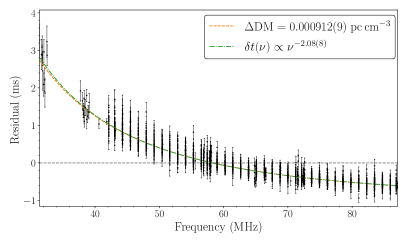
Figure 13: Timing residuals for PSR J1327+3423 which compare LWA1 TOAs to our AO/GBT timing solution are shown, plotted against radio frequency. The dashed gray line shows $\delta t=0$. The curved dashed line shows our fit to the residuals assuming a $\nu^{-2}$ dependence, corresponding to a DM 0.000912(9) pc cm^-3 higher than the fiducial DM used in our timing model (modulo a constant offset). The dotted-dashed line shows a fit which does not make that assumption. The dependence is consistent with a dispersive delay.

It is possible that profile frequency evolution could cause a signature in the residuals which might lead to a mis-estimated DM. The LWA1 TOAs were created using separate (aligned) standard profiles for each of the four center frequencies: 35.1, 49.8, 64.5, and 79.2 MHz, which should account for nearly all of the frequency evolution in the band. Inspecting the relative shapes of the LWA1 pulse profiles, the width of the profile broadens towards lower frequency, but we do not see any other evolution in the shape of the profile within the LWA1 band. In fact, as can be seen from Figure 3, this pulsar’s profile shape is remarkably stable throughout the entire range of observed frequencies, from 35 MHz to over 1.38 GHz.

It is also possible that this effect is due to a frequency-dependent DM. This occurs because radio waves emitted by the pulsar are scattered by the interstellar medium, taking different paths between the pulsar and the Earth. Because the transverse extent of the path lengths varies with frequency, observations at different frequencies sample different regions of the ISM. $\sim$AU-scale electron density fluctuations can then cause DM to vary with frequency (Cordes et al., 2016).

We see strong scintillation in our 820 and 1380 MHz observations of this pulsar. Our observations are not long enough to resolve the scintles in time, but the scintillation bandwidth is $\sim$75 MHz. We did not perform a complete scintillation analysis, so this is a rough estimate. Using equation 12 in Cordes et al. (2016), we can roughly calculate the expected two-frequency DM difference, assuming a Kolmogorov medium and a thin screen. If we take our two frequencies to be $\nu\sim 0.9$ GHz and $\nu^{\prime}=57$ MHz, then we can expect an rms DM difference of order $0.009\,\mathrm{pc\,cm}^{-3}$, which is just within an order of magnitude of our measured DM difference.

5.3 Mildly Recycled Wide Binary Pulsars

PSRs J0032+6946 and J0214+5222 belong to a small group of mildly recycled pulsars in wide binary systems, with orbital periods $P_{\mathrm{b}}>200$ days. There are four other such pulsars: J0407+1607 (Lorimer et al., 2005), J1840$-$0643 (Knispel et al., 2013), J2016+1948 (Navarro et al., 2003), and J2204+2700 (Martinez et al., 2019). The rotational properties of these pulsars imply histories of recycling. This likely occurred when their companion stars entered the giant phase, allowing accretion to occur despite the wide orbital separations. However, perhaps because of the companions’ higher masses, and hence shorter evolutionary timescales, recycling ended before these pulsars could become MSPs (Tauris et al., 2015).

Both pulsars were first published as discoveries in Stovall et al. (2014), but a fully-coherent timing solution did not yet exist for PSR J0032+6946; its binary motion was noticed later. It has a spin period of 37 ms and is in a 523-day, relatively circular ($e\simeq 0.0005$) orbit with a $0.42$ M_☉ $<M_{\mathrm{c}}<1.2$ M_☉ companion, likely a CO-core white dwarf (WD; Tauris, 2011). This range of allowed companion masses is consistent with Tauris & Savonije (1999), who predict the mass of a WD in a $\sim$500-day orbit with a recycled pulsar to be $M_{\mathrm{c}}\sim 0.4-0.45$ M_☉.

Our updated timing solution for PSR J0214+5222 ($P_{\mathrm{b}}\simeq 512$ days, $e\simeq 0.005$ and the same $M_{\mathrm{c}}$ range) is consistent with the Stovall et al. (2014) solution, except for the introduction of two new parameters: $\mu_{\alpha}=9(1)\,\mathrm{mas}\,\textrm{yr}^{-1}$ ($\mu_{\delta}$ is not significant; the best-fit value is 2(2) mas yr^-1 according to PINT), and a secular change in the projected semimajor axis, $\dot{x}_{\mathrm{obs}}=-2.1(6)\times 10^{-13}\;\textrm{s}\,\textrm{s}^{-1}$. Secular changes in $x$ have several potential causes:

$$\dot{x}_{\mathrm{obs}}=\dot{x}_{\mathrm{GW}}+\dot{x}_{\mathrm{PM}}+\dot{x}_{\mathrm{kin}}+\dot{x}_{\dot{m}}+\dot{x}_{\mathrm{prec}}+\dot{x}_{\mathrm{planet}},$$ (8)

where $\dot{x}_{\mathrm{GW}}$ is the contribution from gravitational-wave damping, $\dot{x}_{\mathrm{PM}}$ is caused by the proper motion of the system, $\dot{x}_{\mathrm{kin}}=\dot{x}_{\mathrm{G}}+\dot{x}_{\mathrm{S}}$ is due to the two kinematic effects described in Section 5 (Galactic acceleration, $\dot{x}_{\mathrm{G}}$, and the Shklovskii effect, $\dot{x}_{\mathrm{S}}$), $\dot{x}_{\dot{m}}$ is due to mass loss, $\dot{x}_{\mathrm{prec}}$ is caused by precession (including geodetic precession of the pulsar’s spin axis and orbital precession caused by spin-orbit coupling), and $\dot{x}_{\mathrm{planet}}$ is caused by the deformation of the orbit due to a third body, such as a planet (Lorimer & Kramer, 2004).

We do not expect $\dot{x}_{\dot{m}}$ or $\dot{x}_{\mathrm{prec}}$ to be significant for this pulsar, due to its wide orbit. The contribution from GW damping is $\dot{x}_{\mathrm{GW}}\approx 10^{-26}\;\textrm{s}\,\textrm{s}^{-1}$. For $\dot{x}_{\mathrm{kin}}$, we can use the values for $\dot{P}_{\mathrm{G}}$ and $\dot{P}_{\mathrm{S}}$ reported Table 8 to relate the change in apparent $\dot{P}$ to the variation in $x$ which is caused by the same underlying effects:

$$\dot{x}_{\mathrm{kin}}=-(\dot{P}_{\mathrm{G}}+\dot{P}_{\mathrm{S}})(x/P)\approx 3.5\times 10^{-17}\;\textrm{s}\,\textrm{s}^{-1}.$$ (9)

We cannot rule out the presence of a planetary object. However, to produce the observed $\dot{x}$, a planet would either need to be placed rather conveniently, have an extremely wide orbit ($r\sim 400$ AU) or both (see Equation 8.85 in Lorimer & Kramer, 2004). Assuming no such object exists, the only effect which can explain our observed $\dot{x}$ is a gradual change in the inclination angle of the binary system due to its proper motion.

Measuring this secular variation in $x$, together with that of $\omega$, can allow one to determine $i$ and the longitude of ascending node, $\Omega$ (Kopeikin, 1996). Assuming our measurement is entirely due to proper motion, and that $\mu_{\delta}=0$, we can use Equation 11 in Kopeikin (1996) to say the following:

$$\cot i\sin\Omega=0.9(0.3).$$ (10)

With such high relative uncertainty, we cannot confidently rule out any range of values for $i$. To 68% confidence, $i<59\arcdeg$.

5.4 PSR J1239+3239

PSR J1239+3239 is an MSP with a spin period of 4.7 ms and is in a 4-day orbit with a low-mass companion. Pulsar timing limits the mass of the companion to the range $0.13<M_{\mathrm{c}}<0.31$. This is consistent with the prediction of Tauris & Savonije (1999) for the mass of a WD with this orbital period: $M_{\mathrm{c}}\sim 0.22$ M_☉.

This pulsar has $\delta t_{\mathrm{RMS}}=21.5$ $\mu$s. Furthermore, its wide pulse profile broadens at higher frequencies. Due to these factors, this MSP is unfortunately not suitable for inclusion in PTAs.

5.5 PSR J0636+5128

PSR J0636+5128 (originally known as PSR J0636+5129) is a black widow MSP with a spin period of 2.8 ms in a tight, 1.62 hr orbit with an extremely-light companion: $0.007\,\mathrm{M}_{\odot}<M_{\mathrm{c}}<0.016\,\mathrm{M}_{\odot}$. Assuming $i=60\arcdeg$ and a pulsar mass of $M_{\mathrm{p}}=1.4$ M_☉, $M_{\mathrm{c}}=8.5\,\mathrm{M_{Jupiter}}$. Stovall et al. (2014) proposed this companion as a possible “diamond planet” (e.g., Bailes et al., 2011; Ng & HTRU Collaboration, 2013).

We have measured two significant orbital frequency derivatives (see Table 9); the corresponding derivative of orbital period, $\dot{P}_{\mathrm{b}}=6(1)\times 10^{-12}$, is of the wrong sign and two orders of magnitude too high to be explained by orbital decay from GW emission. Kaplan et al. (2018a) found that kinematic effects due to motion relative to the solar system barycenter also could not explain the measured $\dot{P}_{\mathrm{b}}$. Like in other black widow systems, these orbital frequency derivatives can be explained by tidal and wind effects (Applegate & Shaham, 1994; Chen, 2021).

While fitting for several orbital frequency derivatives is often necessary for black widow systems, this has been shown not to reduce PTAs’ sensitivity to GWs (Bochenek et al., 2015). Furthermore, PSR J0636+5128 does not have radio eclipses, and its timing residuals do not suggest the presence of ionized material in its orbit. Consequently, it has been observed by both NANOGrav and the EPTA (Alam et al., 2021; Desvignes et al., 2016).

Stovall et al. (2014) reported a timing parallax of $\varpi=4.9(6)$ mas for this pulsar; this parameter is not part of our updated solution. With our timing data, tempo2 gives a best-fit value of $\varpi=1.8(1.5)$ mas, which despite not being significant, is consistent with the most recently-published NANOGrav timing solution, which has $\varpi=1.4(2)$ mas (Alam et al., 2021). This change is likely due to our longer data span and use of the DMX model. With a shorter data span, DM variations may have been subsumed into the parallax fit in the Stovall et al. (2014) solution (Kaplan et al., 2018a).

5.6 PSR J1816+4510

PSR J1816+4510 has a spin period of 3.2 ms and is in an 8.66 hr orbit with a $0.16\,\mathrm{M}_{\odot}<M_{\mathrm{c}}<0.41\,$M_☉ companion, consistent with the characteristics of redback systems (Roberts, 2011). See Kaplan et al. (2012) and Stovall et al. (2014) for details on this pulsar’s discovery and initial timing solution, which we are updating in this work. Our updated parameters are largely consistent with the Stovall et al. (2014) solution, with the only significant change being a reduction in $\mu_{\alpha}$ from 5.3(8) to 2(1) mas yr^-1.

PSR J1816+4510 exhibits regular, short-duration eclipses, and the TOAs immediately before and after the eclipse exhibit delays up to 800 $\mu$s due to excess material in the orbit. The delays sharply increase at ingress, and slowly fade to normal post-eclipse over a period nearly as long as the eclipse itself (see the bottom plot of Figure 12). The spectrum of PSR J1816+4510’s companion star is similar to He WDs, but it has the high metallicity and low surface gravity suggestive of a larger, possibly non-degenerate star (Kaplan et al., 2013). It may be that the companion is a bloated proto-He WD which has yet to reach the cooling track Istrate et al. (2014).

Polzin et al. (2020) studied the eclipses of PSR J1816+4510 at 149 and 650 MHz. They showed that eclipses last longer at lower frequencies, lasting for 12.5% of the orbit at 149 MHz compared to 5% at 650 MHz. Contrary to Stovall et al. (2014), they differentiate between the true eclipse (where the pulsar emission disappears entirely) and a “smearing” phase, where additional delays are observed in the TOAs.

To better characterize the eclipse duration and investigate the additional delays during ingress and egress, we producing a single TOA for each 53 s of data (0.17% of the orbit) for our full-orbit GBT observation at 820 MHz, and 4 min (0.77%) for the corresponding 1500 MHz observation. At 820 MHz, the eclipse began at an orbital phase (in units of rotations; otherwise as in Equation 5; superior conjunction occurs at $\phi=0.25$.) of $\phi\approx 0.236$ and lasted until $\phi\approx 0.276$, for a duration of $\approx$ 4% of the orbit, or $\approx$ 21 minutes. At 1500 MHz, eclipse appears to last for $\sim$ 5% of the orbit. However, S/N is low at this frequency, so our ability to differentiate between the “eclipse” and “smearing” phases may be limited. Curiously, the 1500 MHz TOA immediately before eclipse does not appear to have significant additional delay, but the TOA before that does have a large residual, $\delta t\approx 265$ $\mu$s. The two 1500 MHz TOAs after eclipse behave similarly, with the first consistent with zero delay and the next being delayed by $\delta t\approx 135$ $\mu$s.

We see some signs that the length of eclipse varies from orbit to orbit, especially at lower frequencies. We have a lack of orbital phase coverage at 350 MHz from $0.22\lesssim\phi\lesssim 0.32$. We see no excess delay in a 350 MHz observation at $\phi\approx 0.32$, though delays do seem to be present in observations at $\phi\approx 0.35$, from 39 $\mu$s in one observation to 200 $\mu$s in another. Polzin et al. (2020) see similar variations in their 149 MHz observations and suggest they are due to clumping in the tail of material extending from the companion star.

PSR J1816+4510 is associated with the gamma-ray source 4FGL J1816.5+4510. Recently, Clark et al. (2023) reported the discovery of gamma-ray eclipses in several pulsars, including PSR J1816+4510. The existence of such eclipses requires that the companion star directly occult the pulsar, constraining $i$, and thus $M_{\mathrm{p}}$. The constraints they report are $i>79.0\arcdeg$ and allowed ranges $1.64\leq M_{\mathrm{p}}\leq 2.17~{}\mathrm{M}_{\odot}$ and $0.18\leq M_{\mathrm{c}}\leq 0.22~{}\mathrm{M}_{\odot}$ for a Roche-lobe-filling companion, or $i>82.6\arcdeg$ and $1.68\leq M_{\mathrm{p}}\leq 2.11~{}\mathrm{M}_{\odot}$ for a Roche-lobe filling factor of 0.5.

We can use this constraint on $i$ to estimate the companion’s size using the observed eclipse duration at 820 MHz. Assuming $M_{\mathrm{p}}=1.64$ M_☉ and $i=90\arcdeg$, we calculate $a=2.6$ R_☉. The radius for the object which obscures the pulsar for 4% of the orbit is therefore $R_{\mathrm{c}}=0.33$ R_☉. We can also estimate the companion’s Roche lobe radius, $R_{\mathrm{L}}=0.55$ R_☉. These values do not differ greatly in the range $80\arcdeg\leq i\leq 90\arcdeg$. It is therefore clear that PSR J1816+4510’s companion does not extend beyond its Roche lobe, aside from the aforementioned tail of ionized material, which extends for a distance $\sim$ the diameter of the companion.

5.7 Nulling Pulsars

We noticed nulling behavior in each observation of PSRs J0957$-$0619, J2145+2158, and J2210+5712, with nulling periods lasting for a few seconds to a minute for PSR J0957$-$0619, and sometimes several minutes for PSRs J2145+2158 and J2210+5712. Examples of typical observations are shown in Figure 14, clearly showing the evidence for nulling in each pulsar.

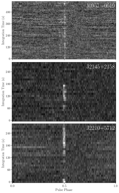
Figure 14: Intensity of pulsar signal vs. time and rotational phase for typical 820 MHz observations of PSRs J0957$-$0619, J2145+2158, and J2210+5712, with greater intensity plotted as brighter and lower intensity plotted as darker. The nulling behavior of each pulsar is readily apparent, with the pulsar signal sometimes disappearing for well over a minute.

We follow Kaplan et al. (2018b); Anumarlapudi et al. (2023) to estimate the nulling fraction using a Gaussian mixture model (GMM). A detailed description is provided in Anumarlapudi et al. (2023); we briefly describe it here. We construct the ON and OFF histograms, which represent the distribution of intensities in a small window around the pulsar’s emission phase and away from the pulsar’s emission phase. These are shown as the dotted and solid histograms in Figure 15.

The OFF histogram is well-described by a Gaussian distribution, as expected for instrumental noise, assuming RFI has been sufficiently removed. We model the ON histogram as a Gaussian mixture of two components—a “null” component and an “emission” component. The intensities in the ON distribution can be thought of as random draws from the emission component when the pulsed emission is observed. When a pulsar nulls, the intensities in the ON distribution will be dominated by the background noise and hence this will be manifested as a scaled version of the OFF distribution, which we call the “null” component. The scale factor is called the nulling fraction (NF) of the pulsar.

The component in the ON histogram that is above the background noise represents the pulsar’s emission and is called the “emission” component. By performing a simultaneous fit for both the ON and OFF histograms, we infer the NF (a detailed explanation of the fitting routine is provided in Anumarlapudi et al. 2023). We find the NF at 820 MHz to be 59.0(2.3)% for PSR J0957$-$0619, 67(2)% for PSR J2145+2158 and 38.8(2.2)% for PSR J2210+5712.

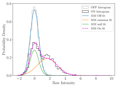
Figure 15: Histograms showing the intensity distributions of the pulsar emission and the background noise for PSR J2210+5712. The dotted and solid histograms show the OFF and ON intensity distributions, respectively. The presence of excess samples in the ON distribution at the level consistent with background noise is evidence for nulling. The blue line shows the Gaussian fit to the OFF histogram. The fit to the ON histogram, shown by the dashed magnenta line, is the sum of the “emission” and “null” components. The emission component (orange line) is a Gaussian centered above the background noise. The null component (green line) is a scaled-down version of the Gaussian noise; this scale factor gives the nulling fraction, which we measure to be $38.8\pm 2.2$% for this pulsar.

PSR J0957$-$0619 was discovered in the 350 MHz Drift-scan survey as a RRAT, with a reported burst rate of 138(29) hr^-1 in a 10-minute GBT observation at 350 MHz (Karako-Argaman et al., 2015). As is apparent from the above analysis, this pulsar is not a RRAT at 820 MHz, instead manifesting as a nulling pulsar. This is further evidence that RRATs may not represent a separate class of neutron star (Burke-Spolaor & Bailes, 2010). Indeed, Cui et al. (2017) showed that RRAT emission likely represents the tail of the normal pulsar intensity distribution.

5.8 Multiwavelength Counterparts

Discussions of the $\gamma$-ray, X-ray, optical, and infrared counterparts of PSRs J0214+5222, J0636+5128, and J1816+4510 can be found in Kaplan et al. (2012), Kaplan et al. (2013), Stovall et al. (2014), Spiewak et al. (2016), and Kaplan et al. (2018a). The temperature of PSR J0214+5222’s companion makes it either a very young WD or a subdwarf B star, and PSR J1816+4510’s companion has properties which indicate it is a bloated proto-WD.

We searched for $\gamma$-ray counterparts of all new discoveries in the Fermi LAT 12-year Source Catalog (4FGL-DR3), finding none. We also used the Aladin server to perform a search for diffuse structures—for example, pulsar wind nebulae (PWN) and supernova remnants (SNRs) that may be associated with the 21 pulsars in this paper. We searched for symmetric diffuse structures expected for bow-shock PWNe (axisymmetric) and SNRs (radially symmetric) using all available imaging data across the electromagnetic spectrum for each pulsar and did find any candidates.

We checked images from the Panoramic Survey Telescope and Rapid Response System (PanSTARRS) $3\pi$ survey (Chambers et al., 2016) at the positions of the new binary pulsars J0032+6946 and J1239+3239, finding no optical counterparts coincident with the pulsars’ timing positions. $r$-band images from the PanSTARRS1 (PS1) public science archive are shown in Figure 16. These undetected companion stars are most likely WDs.

Following previous studies (Lynch et al., 2018; Kaplan et al., 2018a; Swiggum et al., 2023), we use the PS1 nondetections to constrain the effective temperature $T_{\mathrm{eff}}$ and age of PSR J0032+6946’s companion, assuming a CO-core WD. The 5-$\sigma$ grizy magnitude limits are 23.3, 23.2, 23.1, 22.3, and 21.4, respectively (Chambers et al., 2016). Using a 3-D map of interstellar dust (Green et al., 2019), we estimate the reddening to be 0.91 at a distance of 2.8 kpc, corresponding to the DM-derived distance using the NE2001 Galactic electron density model. We use that distance because it is larger than that predicted by the YMW16 model, and so it leads to a more conservative constraint. We convert this to an extinction in each PS1 band using Table 6 in Schlafly & Finkbeiner (2011).

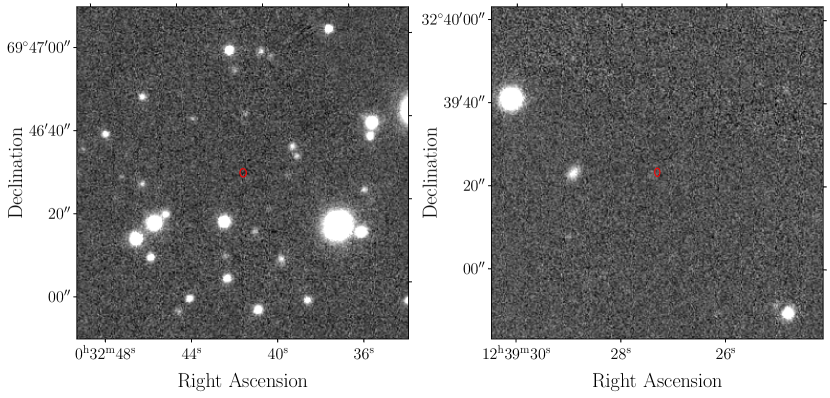
Figure 16: PanSTARRS1 $r$-band images, centered at the positions of PSR J0032+6946 (left) and PSR J1239+3239 (right). The red ellipses represent 1000 $\times$ the uncertainties in the pulsar timing positions. No optical counterparts were found. There is a marginally-detected star near the position of PSR J1239+3239 which also appears in the $i$-band image, but the distance between it and the pulsar is much larger than the frame-time uncertainty ($\sim 0.1\arcsec$).

We compare our magnitude limits to cooling models for a 0.5 M_☉ WD (Bergeron et al., 2011), which is the companion mass assuming that $M_{\mathrm{p}}=1.4$ M_☉ and $i=60\arcdeg$. The $r$-band limit provides the strictest constraints: $T_{\mathrm{eff}}<45000/47500$ K and age $>1.70/1.74$ Myr for hydrogen (DA) / helium (DB) atmospheres.

The lighter companion of PSR J1239+3239 is probably an extremely low-mass (ELM; Brown et al., 2022) He-core WD. Constraining the age is not simple, because hydrogen shell flashes and residual nuclear burning on the surfaces of He WDs lead to non-monotonic cooling (Althaus et al., 2009). Taking the magnitudes given by the Bergeron et al. (2011) cooling models for a 0.2 M_☉ WD, we calculate new magnitudes by scaling the model radius to a range of possible WD radii. We then compare these scaled magnitudes to our magnitude limits to infer the minimum $T_{\mathrm{eff}}$ which PS1 would detect for each radius, using the limit in the band that is most constraining—this varies between $g$, $r$, and $i$. This gives us an upper limit curve constraining $T_{\mathrm{eff}}$, which is shown in Figure 17.

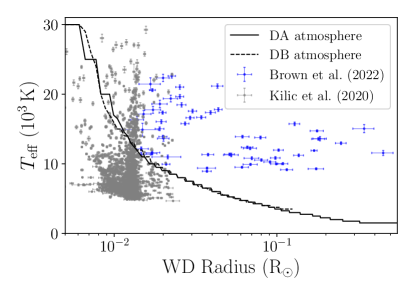
Figure 17: Limits on $T_{\mathrm{eff}}$ for PSR J1239+3239’s $\sim$0.2 M_☉ companion, over a range of typical WD radii. The solid and dashed lines show the limit assuming DA or DB atmospheres, respectively. The gray points show WD radii and effective temperatures from WDs within 100 pc in the SDSS footprint (Brown et al., 2022), and the blue points show values from the ELM Survey (Kilic et al., 2020).

6 Conclusion

We have presented pulse profiles, estimates of flux densities and spectral indices, and timing solutions for 20 pulsars discovered in the GBNCC pulsar survey, and one discovered in the GBT 350 MHz Drift-scan pulsar survey. Three pulsars in our sample (J0141+6303, J1327+3423, and J1434+7257) are DRPs, ejected from their binary systems by their former companion’s supernova. Contrary to what is expected of these systems, the transverse velocities we have measured for PSRs J1327+3423 and J1434+7257 are not particularly high.

PSR J1327+3423 has high timing precision for its spin period, and was observed by the NANOGrav PTA for $\sim$ 2 years at AO. We incorporated these observations into our timing analysis, allowing us to measure proper motion and parallax. We also observed this pulsar using LWA1, and have shown that those observations hint at a chromatic DM, an effect caused by multipath scattering of the pulsar emission through small-scale density fluctuations in the ISM.

We presented new timing solutions for two new binary pulsars: PSR J0032+6946, a mildly recycled pulsar in a wide binary system; and PSR J1239+3239, an MSP orbiting a low-mass WD companion. Their companion stars have masses consistent with the $P_{\mathrm{b}}$–$M_{\mathrm{c}}$ relation for WD companions, but are not seen in archival optical images, leading us to constrain the properties of the WDs. We also presented updated timing solutions for PSR J0214+5222, another mildly recycled wide binary pulsar for which we weakly constrain $i$; PSR J0636+5128, a non-eclipsing black widow MSP which is observed by PTA experiments searching for low-frequency GWs; and PSR J1816+4510, an eclipsing binary MSP with a redback-mass companion.

We also analyzed three nulling pulsars using a Gaussian Mixture method. One of these pulsars, J0957$-$0619, was discovered as a RRAT at 350 MHz. This is further evidence that RRATs may represent the tail of the intensity distribution of the general pulsar population.

The GBNCC pulsar survey has found 194 new pulsars in its coverage of the entire 350 MHz GBT sky. Follow-up timing of GBNCC discoveries continues at the Canadian Hydrogen Intensity Mapping Experiment (CHIME) telescope, thanks to collaboration between GBNCC and CHIME$-$Pulsar (CHIME/Pulsar Collaboration et al., 2021). Results from that effort will be presented in a future work.

References

- Agazie et al. (2021) Agazie, G. Y., Mingyar, M. G., McLaughlin, M. A., et al. 2021, ApJ, 922, 35, doi: 10.3847/1538-4357/ac142b
- Alam et al. (2021) Alam, M. F., Arzoumanian, Z., Baker, P. T., et al. 2021, ApJS, 252, 4, doi: 10.3847/1538-4365/abc6a0
- Aloisi et al. (2019) Aloisi, R. J., Cruz, A., Daniels, L., et al. 2019, ApJ, 875, 19, doi: 10.3847/1538-4357/ab0d21
- Alpar et al. (1982) Alpar, M. A., Cheng, A. F., Ruderman, M. A., & Shaham, J. 1982, Nature, 300, 728, doi: 10.1038/300728a0
- Althaus et al. (2009) Althaus, L. G., Panei, J. A., Romero, A. D., et al. 2009, A&A, 502, 207, doi: 10.1051/0004-6361/200911640
- Antoniadis et al. (2022) Antoniadis, J., Arzoumanian, Z., Babak, S., et al. 2022, MNRAS, 510, 4873, doi: 10.1093/mnras/stab3418
- Anumarlapudi et al. (2023) Anumarlapudi, A., Swiggum, J. K., Kaplan, D. L., & Fichtenbauer, T. D. J. 2023, ApJ, 948, 32, doi: 10.3847/1538-4357/acbb68
- Applegate & Shaham (1994) Applegate, J. H., & Shaham, J. 1994, ApJ, 436, 312, doi: 10.1086/174906
- Archibald et al. (2018) Archibald, A. M., Gusinskaia, N. V., Hessels, J. W. T., et al. 2018, Nature, 559, 73, doi: 10.1038/s41586-018-0265-1
- Astropy Collaboration et al. (2022) Astropy Collaboration, Price-Whelan, A. M., Lim, P. L., et al. 2022, ApJ, 935, 167, doi: 10.3847/1538-4357/ac7c74
- Bailes et al. (2011) Bailes, M., Bates, S. D., Bhalerao, V., et al. 2011, Science, 333, 1717, doi: 10.1126/science.1208890
- Barr et al. (2013) Barr, E. D., Champion, D. J., Kramer, M., et al. 2013, MNRAS, 435, 2234, doi: 10.1093/mnras/stt1440
- Belczynski et al. (2010) Belczynski, K., Lorimer, D. R., Ridley, J. P., & Curran, S. J. 2010, MNRAS, 407, 1245, doi: 10.1111/j.1365-2966.2010.16970.x
- Bergeron et al. (2011) Bergeron, P., Wesemael, F., Dufour, P., et al. 2011, ApJ, 737, 28, doi: 10.1088/0004-637X/737/1/28
- Blandford & Teukolsky (1976) Blandford, R., & Teukolsky, S. A. 1976, ApJ, 205, 580, doi: 10.1086/154315
- Bochenek et al. (2015) Bochenek, C., Ransom, S., & Demorest, P. 2015, ApJ, 813, L4, doi: 10.1088/2041-8205/813/1/L4
- Brown et al. (2022) Brown, W. R., Kilic, M., Kosakowski, A., & Gianninas, A. 2022, ApJ, 933, 94, doi: 10.3847/1538-4357/ac72ac
- Burke-Spolaor & Bailes (2010) Burke-Spolaor, S., & Bailes, M. 2010, MNRAS, 402, 855, doi: 10.1111/j.1365-2966.2009.15965.x
- Chambers et al. (2016) Chambers, K. C., Magnier, E. A., Metcalfe, N., et al. 2016, arXiv e-prints, arXiv:1612.05560, doi: 10.48550/arXiv.1612.05560
- Chen et al. (2013) Chen, H.-L., Chen, X., Tauris, T. M., & Han, Z. 2013, ApJ, 775, 27, doi: 10.1088/0004-637X/775/1/27
- Chen (2021) Chen, W.-C. 2021, MNRAS, 501, 2327, doi: 10.1093/mnras/staa3701
- CHIME/Pulsar Collaboration et al. (2021) CHIME/Pulsar Collaboration, Amiri, M., Bandura, K. M., et al. 2021, ApJS, 255, 5, doi: 10.3847/1538-4365/abfdcb
- Clark et al. (2023) Clark, C. J., Kerr, M., Barr, E. D., et al. 2023, Nature Astronomy, doi: 10.1038/s41550-022-01874-x
- Cordes & Lazio (2002) Cordes, J. M., & Lazio, T. J. W. 2002, arXiv e-prints, astro. https://arxiv.org/abs/astro-ph/0207156
- Cordes & Lazio (2003) —. 2003, arXiv e-prints, astro. https://arxiv.org/abs/astro-ph/0301598
- Cordes et al. (2016) Cordes, J. M., Shannon, R. M., & Stinebring, D. R. 2016, ApJ, 817, 16, doi: 10.3847/0004-637X/817/1/16
- Cromartie et al. (2020) Cromartie, H. T., Fonseca, E., Ransom, S. M., et al. 2020, Nature Astronomy, 4, 72, doi: 10.1038/s41550-019-0880-2
- Cui et al. (2017) Cui, B. Y., Boyles, J., McLaughlin, M. A., & Palliyaguru, N. 2017, ApJ, 840, 5, doi: 10.3847/1538-4357/aa6aa9
- Deller et al. (2019) Deller, A. T., Goss, W. M., Brisken, W. F., et al. 2019, ApJ, 875, 100, doi: 10.3847/1538-4357/ab11c7
- Desvignes et al. (2016) Desvignes, G., Caballero, R. N., Lentati, L., et al. 2016, MNRAS, 458, 3341, doi: 10.1093/mnras/stw483
- Ellingson et al. (2013) Ellingson, S. W., Taylor, G. B., Craig, J., et al. 2013, IEEE Transactions on Antennas and Propagation, 61, 2540, doi: 10.1109/TAP.2013.2242826
- Fonseca et al. (2021) Fonseca, E., Cromartie, H. T., Pennucci, T. T., et al. 2021, ApJ, 915, L12, doi: 10.3847/2041-8213/ac03b8
- Fruchter et al. (1988) Fruchter, A. S., Stinebring, D. R., & Taylor, J. H. 1988, Nature, 333, 237, doi: 10.1038/333237a0
- GRAVITY Collaboration et al. (2021) GRAVITY Collaboration, Abuter, R., Amorim, A., et al. 2021, A&A, 647, A59, doi: 10.1051/0004-6361/202040208
- Green et al. (2019) Green, G. M., Schlafly, E., Zucker, C., Speagle, J. S., & Finkbeiner, D. 2019, ApJ, 887, 93, doi: 10.3847/1538-4357/ab5362
- Guo et al. (2021) Guo, Y. J., Freire, P. C. C., Guillemot, L., et al. 2021, A&A, 654, A16, doi: 10.1051/0004-6361/202141450
- Harris et al. (2020) Harris, C. R., Millman, K. J., van der Walt, S. J., et al. 2020, Nature, 585, 357, doi: 10.1038/s41586-020-2649-2
- Hobbs & Edwards (2012) Hobbs, G., & Edwards, R. 2012, Tempo2: Pulsar Timing Package, Astrophysics Source Code Library, record ascl:1210.015. http://ascl.net/1210.015
- Hobbs et al. (2012) Hobbs, G., Coles, W., Manchester, R. N., et al. 2012, MNRAS, 427, 2780, doi: 10.1111/j.1365-2966.2012.21946.x
- Hobbs et al. (2020) Hobbs, G., Guo, L., Caballero, R. N., et al. 2020, MNRAS, 491, 5951, doi: 10.1093/mnras/stz3071
- Hobbs et al. (2006) Hobbs, G. B., Edwards, R. T., & Manchester, R. N. 2006, MNRAS, 369, 655, doi: 10.1111/j.1365-2966.2006.10302.x
- Holmberg & Flynn (2004) Holmberg, J., & Flynn, C. 2004, MNRAS, 352, 440, doi: 10.1111/j.1365-2966.2004.07931.x
- Hotan et al. (2004) Hotan, A. W., van Straten, W., & Manchester, R. N. 2004, PASA, 21, 302, doi: 10.1071/AS04022
- Hunter (2007) Hunter, J. D. 2007, Computing in Science & Engineering, 9, 90, doi: 10.1109/MCSE.2007.55
- Istrate et al. (2014) Istrate, A. G., Tauris, T. M., Langer, N., & Antoniadis, J. 2014, A&A, 571, L3, doi: 10.1051/0004-6361/201424681
- Jones et al. (2017) Jones, M. L., McLaughlin, M. A., Lam, M. T., et al. 2017, ApJ, 841, 125, doi: 10.3847/1538-4357/aa73df
- Kaplan et al. (2013) Kaplan, D. L., Bhalerao, V. B., van Kerkwijk, M. H., et al. 2013, ApJ, 765, 158, doi: 10.1088/0004-637X/765/2/158
- Kaplan et al. (2018a) Kaplan, D. L., Stovall, K., van Kerkwijk, M. H., Fremling, C., & Istrate, A. G. 2018a, ApJ, 864, 15, doi: 10.3847/1538-4357/aad54c
- Kaplan et al. (2018b) Kaplan, D. L., Swiggum, J. K., Fichtenbauer, T. D. J., & Vallisneri, M. 2018b, ApJ, 855, 14, doi: 10.3847/1538-4357/aaab62
- Kaplan et al. (2012) Kaplan, D. L., Stovall, K., Ransom, S. M., et al. 2012, The Astrophysical Journal, 753, 174, doi: 10.1088/0004-637x/753/2/174
- Karako-Argaman et al. (2015) Karako-Argaman, C., Kaspi, V. M., Lynch, R. S., et al. 2015, ApJ, 809, 67, doi: 10.1088/0004-637X/809/1/67
- Kawash et al. (2018) Kawash, A. M., McLaughlin, M. A., Kaplan, D. L., et al. 2018, ApJ, 857, 131, doi: 10.3847/1538-4357/aab61d
- Kilic et al. (2020) Kilic, M., Bergeron, P., Kosakowski, A., et al. 2020, ApJ, 898, 84, doi: 10.3847/1538-4357/ab9b8d
- Knispel et al. (2013) Knispel, B., Eatough, R. P., Kim, H., et al. 2013, ApJ, 774, 93, doi: 10.1088/0004-637X/774/2/93
- Kondratiev et al. (2016) Kondratiev, V. I., Verbiest, J. P. W., Hessels, J. W. T., et al. 2016, A&A, 585, A128, doi: 10.1051/0004-6361/201527178
- Kopeikin (1996) Kopeikin, S. M. 1996, ApJ, 467, L93, doi: 10.1086/310201
- Kramer et al. (2021) Kramer, M., Stairs, I. H., Manchester, R. N., et al. 2021, Physical Review X, 11, 041050, doi: 10.1103/PhysRevX.11.041050
- Lange et al. (2001) Lange, C., Camilo, F., Wex, N., et al. 2001, MNRAS, 326, 274, doi: 10.1046/j.1365-8711.2001.04606.x
- Lorimer & Kramer (2004) Lorimer, D. R., & Kramer, M. 2004, Handbook of Pulsar Astronomy (UK: Cambridge University Press)
- Lorimer et al. (2004) Lorimer, D. R., McLaughlin, M. A., Arzoumanian, Z., et al. 2004, MNRAS, 347, L21, doi: 10.1111/j.1365-2966.2004.07407.x
- Lorimer et al. (2005) Lorimer, D. R., Xilouris, K. M., Fruchter, A. S., et al. 2005, Monthly Notices of the Royal Astronomical Society, 359, 1524, doi: 10.1111/j.1365-2966.2005.09005.x
- Luo et al. (2021) Luo, J., Ransom, S., Demorest, P., et al. 2021, ApJ, 911, 45, doi: 10.3847/1538-4357/abe62f
- Lynch et al. (2018) Lynch, R. S., Swiggum, J. K., Kondratiev, V. I., et al. 2018, ApJ, 859, 93, doi: 10.3847/1538-4357/aabf8a
- Manchester et al. (2005) Manchester, R. N., Hobbs, G. B., Teoh, A., & Hobbs, M. 2005, AJ, 129, 1993, doi: 10.1086/428488
- Martinez et al. (2019) Martinez, J. G., Gentile, P., Freire, P. C. C., et al. 2019, ApJ, 881, 166, doi: 10.3847/1538-4357/ab2877
- McEwen et al. (2020) McEwen, A. E., Spiewak, R., Swiggum, J. K., et al. 2020, ApJ, 892, 76, doi: 10.3847/1538-4357/ab75e2
- McLaughlin et al. (2006) McLaughlin, M. A., Lyne, A. G., Lorimer, D. R., et al. 2006, Nature, 439, 817, doi: 10.1038/nature04440
- NANOGrav Collaboration et al. (2015) NANOGrav Collaboration, Arzoumanian, Z., Brazier, A., et al. 2015, ApJ, 813, 65, doi: 10.1088/0004-637X/813/1/65
- Navarro et al. (2003) Navarro, J., Anderson, S. B., & Freire, P. C. 2003, ApJ, 594, 943, doi: 10.1086/377153
- Ng & HTRU Collaboration (2013) Ng, C., & HTRU Collaboration. 2013, in Neutron Stars and Pulsars: Challenges and Opportunities after 80 years, ed. J. van Leeuwen, Vol. 291, 53–56, doi: 10.1017/S1743921312023137
- Parent et al. (2020) Parent, E., Chawla, P., Kaspi, V. M., et al. 2020, ApJ, 904, 92, doi: 10.3847/1538-4357/abbdf6
- Perera et al. (2019) Perera, B. B. P., DeCesar, M. E., Demorest, P. B., et al. 2019, MNRAS, 490, 4666, doi: 10.1093/mnras/stz2857
- Polzin et al. (2020) Polzin, E. J., Breton, R. P., Bhattacharyya, B., et al. 2020, MNRAS, 494, 2948, doi: 10.1093/mnras/staa596
- Polzin et al. (2018) Polzin, E. J., Breton, R. P., Clarke, A. O., et al. 2018, MNRAS, 476, 1968, doi: 10.1093/mnras/sty349
- Price (2016) Price, D. C. 2016, PyGSM: Python interface to the Global Sky Model, Astrophysics Source Code Library, record ascl:1603.013. http://ascl.net/1603.013
- Price et al. (2021) Price, D. C., Flynn, C., & Deller, A. 2021, PASA, 38, e038, doi: 10.1017/pasa.2021.33
- Ransom et al. (2009) Ransom, S. M., Demorest, P., Ford, J., et al. 2009, in American Astronomical Society Meeting Abstracts, Vol. 214, American Astronomical Society Meeting Abstracts #214, 605.08
- Ransom et al. (2002) Ransom, S. M., Eikenberry, S. S., & Middleditch, J. 2002, AJ, 124, 1788, doi: 10.1086/342285
- Roberts (2011) Roberts, M. S. E. 2011, in American Institute of Physics Conference Series, Vol. 1357, Radio Pulsars: An Astrophysical Key to Unlock the Secrets of the Universe, ed. M. Burgay, N. D’Amico, P. Esposito, A. Pellizzoni, & A. Possenti, 127–130, doi: 10.1063/1.3615095
- Schlafly & Finkbeiner (2011) Schlafly, E. F., & Finkbeiner, D. P. 2011, ApJ, 737, 103, doi: 10.1088/0004-637X/737/2/103
- Shklovskii (1970) Shklovskii, I. S. 1970, Soviet Ast., 13, 562
- Spiewak et al. (2016) Spiewak, R., Kaplan, D. L., Archibald, A., et al. 2016, ApJ, 822, 37, doi: 10.3847/0004-637X/822/1/37
- Stovall et al. (2014) Stovall, K., Lynch, R. S., Ransom, S. M., et al. 2014, ApJ, 791, 67, doi: 10.1088/0004-637X/791/1/67
- Swiggum et al. (2023) Swiggum, J. K., Pleunis, Z., Parent, E., et al. 2023, ApJ, 944, 154, doi: 10.3847/1538-4357/acb43f
- Tauris (2011) Tauris, T. M. 2011, in Astronomical Society of the Pacific Conference Series, Vol. 447, Evolution of Compact Binaries, ed. L. Schmidtobreick, M. R. Schreiber, & C. Tappert, 285, doi: 10.48550/arXiv.1106.0897
- Tauris et al. (2015) Tauris, T. M., Langer, N., & Podsiadlowski, P. 2015, MNRAS, 451, 2123, doi: 10.1093/mnras/stv990
- Tauris & Savonije (1999) Tauris, T. M., & Savonije, G. J. 1999, A&A, 350, 928, doi: 10.48550/arXiv.astro-ph/9909147
- Taylor (1992) Taylor, J. H. 1992, Philosophical Transactions of the Royal Society of London Series A, 341, 117, doi: 10.1098/rsta.1992.0088
- van Haarlem et al. (2013) van Haarlem, M. P., Wise, M. W., Gunst, A. W., et al. 2013, A&A, 556, A2, doi: 10.1051/0004-6361/201220873
- van Straten et al. (2011) van Straten, W., Demorest, P., Khoo, J., et al. 2011, PSRCHIVE: Development Library for the Analysis of Pulsar Astronomical Data, Astrophysics Source Code Library, record ascl:1105.014. http://ascl.net/1105.014
- Verbiest et al. (2010) Verbiest, J. P. W., Lorimer, D. R., & McLaughlin, M. A. 2010, MNRAS, 405, 564, doi: 10.1111/j.1365-2966.2010.16488.x
- Virtanen et al. (2020) Virtanen, P., Gommers, R., Oliphant, T. E., et al. 2020, Nature Methods, 17, 261, doi: 10.1038/s41592-019-0686-2
- Yamasaki & Totani (2020) Yamasaki, S., & Totani, T. 2020, ApJ, 888, 105, doi: 10.3847/1538-4357/ab58c4
- Yao et al. (2017) Yao, J. M., Manchester, R. N., & Wang, N. 2017, ApJ, 835, 29, doi: 10.3847/1538-4357/835/1/29
- Zheng et al. (2017) Zheng, H., Tegmark, M., Dillon, J. S., et al. 2017, MNRAS, 464, 3486, doi: 10.1093/mnras/stw2525
- Zhu et al. (2019) Zhu, W. W., Desvignes, G., Wex, N., et al. 2019, MNRAS, 482, 3249, doi: 10.1093/mnras/sty2905