A reduced-order model for segregated fluid-structure interaction solvers based on an ALE approach

Abstract

This article presents a Galerkin projection model order reduction approach for fluid-structure interaction (FSI) problems in the Finite Volume context. The reduced-order model (ROM) is based on proper orthogonal decomposition (POD), where a reduced basis is formed using energy-dominant POD modes. The reduced basis also consists of characteristics of the POD time modes derived from the POD time modes coefficients. In addition, the solution state vector comprises the mesh deformation, considering the structural motion in FSI. The results are obtained by applying the proposed method to time-dependent problems governed by the 2D incompressible Navier-Stokes equations. The main objective of this work is to introduce a hybrid technique mixing up the classical Galerkin-projection approach with a data-driven method to obtain a versatile and accurate algorithm for resolving FSI problems with moving meshes. The effectiveness of this approach is demonstrated in the case study of vortex-induced vibrations (VIV) of a cylinder at Reynolds number $Re=200$. The results show the stability and accuracy of the proposed method with respect to the high-dimensional model by capturing transient flow fields and, more importantly, the forces acting on the moving objects.

Keywords: Fluid-structure interaction, reduced-order model, Finite Volume Method, Proper Orthogonal Decomposition, Galerkin projection, radial basis network, mesh motion.

1 Motivation and state-of-the-art

Several significant problems require fluid-structure interaction (FSI) understanding. The reason is that the interaction of a fluid with some movable or deformable structure has historical and practical importance, and it is considered in the design of many engineering systems [9, 7]. Bluff bodies (cylinder, prism, square, etc…) in general, are exposed to streams (flows) and they are found in bridges, chimney stacks, marine cables, water and gas pipelines and understanding theirs dynamics have been an essential task in the engineering community as they represent a selection of engineering structures known to undergo significant vibrations when subjected to the flow of air or water. As a result, the topic has attracted an increasing attention from the research community since the middle of the twentieth century [21]. To model such a large variety of applications (mentioned above) in the computer, the flow past a circular cylinder has been a benchmark problem in fluid dynamics that serves to simulate and understand those types of applications[36, 35]and has indeed provided a “kaleidoscope of challenging, fluid phenomena [6].“ Generally, it is a significant challenge when dealing with FSI problems because, all numerical simulations evolving them (FSI problems) are computationally expensive (for data storage, data handling, and processing costs), even when implemented on modern advanced computing platforms. Given this difficulty, we pay significant attention to reducing both storage and processing costs of non-linear state solutions by using reduced-order models (ROMs) [11]. A ROM is a mathematical model of a physical system derived from computational or, at times, even experimental data. The ROM contains fewer degrees of freedom than the discretized partial differential equations, and it results, therefore, in relatively inexpensive simulations. ROMs are developed and used to provide a more efficient and computationally economical way of investigating these complex problems. The use of ROMs is primarily motivated by the desire to have detailed knowledge of the physics of the problem being investigated together with an efficient and reliable prediction tool [28]. Various methods of building reduced-order models exist. The common underlying theme is to extract the key features in the flow field, preferably from a high-fidelity experimental or computational data source. The extracted features are carefully chosen to represent dominant spatiotemporal dynamics as computed using the Navier-Stokes equations.

In the model reduction family, POD-Galerkin (POD-G) projection is one of the most popular approaches because it has succeeded in various research areas [2]. Several scholars have widely studied the application of ROMs for fluid-structure interaction, and state-of-the-art counts already several scientific contributions. In [32], the authors presented an overview of the combination of the Reduced Basis Method (RBM) with two different approaches for fluid-structure interaction (FSI) problems, namely, a monolithic and a partitioned approach. They provided a detailed implementation of the two reduction procedures and then applied them to the Turek–Hron benchmark test case with a fluid Reynolds number Re = 100. An optimization-based domain-decomposition reduced-order model for the incompressible Navier-Stokes equations has been examined in [37]. The methodology has been tested on two fluid dynamics benchmarks: the stationary backward-facing step and lid-driven cavity flow. The numerical tests significantly reduced computational costs regarding the problem dimensions and the number of optimization iterations in the domain-decomposition algorithm. Researchers in [53] have made some improvements to extend the application of POD-Galerkin projection to a domain with moving solid boundaries or structures. In [27, 9], the authors chose to apply the immersed interface method with POD on a flow passing an oscillatory cylinder. They simulated the interaction between a fluid and a rigid body with imposed rotation velocity. A Galerkin-free ROM approach based on POD has been applied to FSI problems with large mesh deformations in [43]. The authors used a two-dimensional VIV on a cylinder and a three-dimensional shock wave boundary layer-induced panel flutter to demonstrate their methodology; due to the numerical issues associated with Galerkin ROM and the difficulty of constructing a ROM for FSI problem with the moving mesh, the authors have used two separate ROM for the fluid and the structure domain. The study conducted in [52] discussed a non-intrusive reduced order model (NIROM) for FSI. The authors based their method on POD and radial basis functions (RBF) interpolation method for unstructured meshes in the finite element method setting. One of the advantages of the non-intrusive method is that it is independent of the governing equations. They validated their methodology on a one-way coupling (flow past a cylinder), a two-way coupling (a free-falling cylinder in water), and vortex-induced vibrations of an elastic beam. Their methodology has shown outstanding performance. The scholars in [42] proposed a decoupled modeling of the FSI problem; they modeled the fluid and structure domains separately. They constructed POD-ROM global basis function for the structure using the singular value decomposition (SVD). In the work of Liberge and Hamdouni [26], extended from their previous work on the 1-D Burgers equation [25], defined global POD modes from a global fluid-solid velocity field, and successfully built a ROM for the flow passing a spring-attached cylinder oscillating at a small amplitude. Several approaches for constructing hybrid ROM and Machine Learning are also explored in the literature in [13, 34, 51, 29, 30] as a potential way to circumvent the stability issues associated Galerkin projection. It is worth mentioning that all the methodologies mentioned earlier used Finite Element Method (FEM) as a full-order model.

Recent works have been done in the framework of reduced-order models with the Finite Volume Method in [14, 47, 46, 17, 4]. The work addressed in [4] proposed a ROM approach for transient modeling multiple objects in nonlinear cross-flows. The latter modeled a technique based on the moving domain and immersed boundary method to overcome the challenge of handling moving boundaries due to the movements of multiple objects. This work differs from the works mentioned above by considering the motion of the mesh in the Arbitrary Lagrangian-Eulerian (ALE) sense and proposes a hybrid approach where the main partial differential equations (PDEs) are treated using a standard POD-Galerkin projection approach and partially radial basis functions networks data-driven approaches for point cloud interpolation respectively. This choice is based on both theoretical studies and practical considerations. The practical aspects are related to the idea of generating an approach that could be applied to the mesh motion model (see Subsection 2.4). Secondly, despite a large amount of theoretical work behind the mesh motion model, there are still several empirical coefficients, making the overall formulation less rigorous in terms of physical principles. These considerations have been used to propose a reduced-order model that could be applied to any mesh motion model that exploits a projection-based technique for mass and momentum conservation and a data-driven approach for reconstructing the point displacement field. This work considers a cross-flow of Reynolds number $Re=200$. Although the test case is relatively simplified compared to realistic problems, this study is among the few attempts to extend ROM’s capability to model moving objects in the Finite Volume platform and capture the forces acting on the object. The development of ROM for simulations of high Re flow is beyond the focus of this paper. It is currently conducted in a separate analysis by the authors on different benchmark problems.

The manuscript is organized as follows: Section 2 begins with the formulation of the structure dynamic (see Subsection 2.1). In the next three subsections, the mathematical formulation of the fluid’s motion in the ALE setting is presented (see Subsection 2.2), followed by the coupling strategy at the interface (see Subsection 2.3) and Subsection 2.4 discusses some mesh motion strategies. Section 3 starts by addressing the numerical discretization of the full-order model (see Subsection 3.1), then Subsection 3.2 addresses the reduced-order model concept; follows with the discussion of Proper Orthogonal Decomposition (POD) for laminar incompressible flows in Subsection 3.3 by insisting on its main properties in terms of model reduction while Subsection 3.4 formally introduces the POD-RBF with radial basis functions networks. Section 4 discusses and presents the numerical results. In the end, a few considerations and possible future developments for this work are present in Section 5.

2 Mathematical formulation of the fluid-structure interaction problem

This section presents the mathematical formulation of the fluid-structure interaction model. The following assumptions are made:

• The fluid is viscous, incompressible and Newtonian,

• A 2D simulation is carried out,

• The cylindrical structure is rigid. Its elastic connection to the ground is represented by a spring and a damper,

• The cylinder is free to oscillate in the vertical direction.

When dealing with fluid-structure interaction problems, several questions arise about the coupling algorithm, the mesh moving strategy, the Galilean Invariance of the scheme, and compliance with the Discrete Geometric Conservation Law (DGCL). Therefore, based on the assumptions mentioned above, the present part briefly describes the high-dimensional full-order model to simulate the coupled fluid-body interaction using the Navier-Stokes equations in the ALE setting, considering the rigid body dynamics and the coupling conditions at the interface.

2.1 Formulation for structural dynamics

Cauchy’s equation gives the equation governing the dynamics of the solid structure described:

$$\ddot{y}+2\zeta\omega_{n}\dot{y}+\omega^{2}_{n}y=\frac{F_{y}}{m}.$$ (1)

Where $\omega_{n}=\sqrt{\dfrac{k}{m}}=2\pi f_{n}$ is the natural pulsation of the system, $k$ is the spring’s stiffness, $m$ is the mass of the rigid body, $\zeta=\dfrac{c}{2m\omega_{n}}$ is the fraction of structural damping $c$ with respect to critical or simply damping ratio, $y$ is the displacement of the cylinder in the transverse direction, and $F_{y}$ is the lift force in the free-stream transverse direction. The fluid force $F_{y}$ per unit length of the cylinder drives the motion of the cylinder.

2.2 Formulation for fluid dynamics

In order to cope with the continuous motion of the structure, the computational grid for the fluid flow is allowed to move accordingly. The momentum equation in the ALE framework is written as follows:

$$\frac{\delta\bm{u}}{\delta t}+\nabla\cdot[\bm{u}\otimes(\bm{u}-\bm{u}_{g})]-\nabla\cdot(\mu\nabla\bm{u})=-\nabla p.$$ (2)

With $\bm{u}=[u,v]^{T}$, $\bm{u}_{g}=[u_{g},v_{g}]^{T}$, $p$ and $\mu$ being respectively the fluid velocity, the grid velocity (boundary mesh), the pressure, and the dynamic viscosity. Several Computational Fluid Dynamics (CFD) packages are available to solve the above governing Partial Differential Equations (PDEs), such as Fluent, StarCCM (commercial), or OpenFOAM (open-source). The time derivative for a given field $\phi$ in the ALE framework is given by:

$$\frac{\delta\phi}{\delta t}=\frac{\partial\phi}{\partial t}+\bm{u}_{g}\nabla\phi.$$ (3)

Additionally,

$$\nabla\cdot\bm{u}=0.$$ (4)

represent the continuity equation. The grid which moves in space must also obey the conservation law [48], which is stated as ”the change in volume (area) of each control volume between time $t^{n}$ and $t^{n+1}$ must equal the volume (area) swept by the cell’s boundary during $\Delta t=t^{n+1}-t^{n}$ which may be expressed as:

$$\frac{\delta}{\delta t}\int_{\Omega_{i}}dV+\int_{\partial\Omega_{i}}\bm{u}_{g}\cdot\bm{n}dS=0\leavevmode\nobreak\ \leavevmode\nobreak\ \leavevmode\nobreak\ \equiv\leavevmode\nobreak\ \leavevmode\nobreak\ \leavevmode\nobreak\ \displaystyle\frac{\delta\Omega_{i}}{\delta t}+\nabla\cdot\bm{u}_{g}=0,$$ (5)

for every control volume $\Omega_{i}=\Omega_{i}(t)$. $\bm{n}$ is the outward unit normal vector on the boundary surface. By multiplying Equation 5 by $\rho$ and using the incompressibility constraint leads to:

$$\int_{\partial\Omega_{i}}\bm{u}_{g}\cdot\bm{n}dS=0.$$ (6)

This means there is no need to consider the grid velocity in the continuity Equation 4. For a well-posed problem, the above equations are supplemented by appropriate initial and boundaries conditions, and $\bm{u}_{g}$ satisfy the following conditions: $\begin{cases}v_{g}=\dot{y}\leavevmode\nobreak\ \leavevmode\nobreak\ \leavevmode\nobreak\ \leavevmode\nobreak\ \text{on}\leavevmode\nobreak\ \leavevmode\nobreak\ \leavevmode\nobreak\ \leavevmode\nobreak\ \Gamma_{I}(t)\\ v_{g}=0\leavevmode\nobreak\ \leavevmode\nobreak\ \leavevmode\nobreak\ \leavevmode\nobreak\ \text{on}\leavevmode\nobreak\ \leavevmode\nobreak\ \leavevmode\nobreak\ \leavevmode\nobreak\ \partial\Omega\setminus\Gamma_{I}(t)\end{cases}$ with, $\Gamma_{I}(t)$ the cylinder interface.

2.3 Coupling conditions at the interface

$$v=v_{g}=\dot{y}\leavevmode\nobreak\ \leavevmode\nobreak\ \leavevmode\nobreak\ \text{and}\leavevmode\nobreak\ \leavevmode\nobreak\ \leavevmode\nobreak\ \int_{\Gamma(t)}(\bm{\sigma}_{f}(\bm{x},t)\cdot\bm{n})\cdot\bm{n}_{y}d\Gamma+F_{y}=0,$$ (7)

with $\bm{\sigma}_{f}(\bm{x},t)=-p(\bm{x},t)\mathbf{I}+\mu\left(\nabla\cdot\bm{u}(\bm{x},t)+\left(\nabla\cdot\bm{u}(\bm{x},t)\right)^{T}\right)$ as it is assumed that the fluid is Newtonian.

2.4 Mesh motion strategies

The Arbitrary Lagrangian-Eulerian (ALE) formulation is used to treat all the possible different geometric configurations. Therefore, the shape of the computational domain changes according to the cylinder’s displacement. In the framework of the FSI problem, the position of the body boundary mesh points in the fluid domain is obtained by solving the structural problem. On the other hand, the fluid domain’s internal grid points must be displaced to preserve mesh quality and avoid negative volume or skewed cells. Dealing with a full-order finite volume discretization, we highlight here, as seen in the description of the full-order discretization, that the accuracy of the solution is strongly dependent on the quality of the mesh. For this reason, in selecting the mesh motion strategy, it is crucial to select an algorithm that produces a deformed mesh with a non-orthogonality value as small as possible. The interested reader may refer to [40, 20, 5] and to references therein for more details.

2.4.1 Mesh deformation: linear spring analogy technique

One of the popular methods in the class of the physical analogy approach is the tension spring analogy. In this approach, each mesh edge is replaced by a tension spring, with the spring stiffness taken inversely proportional to the edge length. The physical analogy approach is more suitable for users and small geometries or two-dimensional problems; when performing the mesh deformation task repeatedly, for large-scale problems, the physical analogy approach will exhibit overwhelming computational resources. This approach can be a good option if the mesh deformation task is required once. Many researchers have adopted the spring analogy and used the same assumption for stiffness. In this method, the equilibrium lengths of the springs are set equal to the initial lengths of the edges [40]. By applying Hook’s law to the displacements of the nodes, the force is written as:

$$\bm{F}_{i}=\displaystyle\sum_{j=1}^{N_{i}}\alpha_{ij}(\bm{\delta}_{j}-\bm{\delta}_{i}).$$ (8)

Where $\alpha_{ij}$ is the stiffness of the spring between node i and j, $\bm{\delta}$ is the node displacement, and $N_{i}$ is the number of neighbors of node i. For static equilibrium, the force at every node $i$ has to be zero. The iterative equation to be solved is

$$\bm{\delta}_{i}^{k+1}=\displaystyle\frac{\displaystyle\sum_{j=1}^{N_{i}}\alpha_{ij}\bm{\delta}_{j}^{k}}{\displaystyle\sum_{j=1}^{N_{i}}\alpha_{ij}},$$ (9)

where the known displacements at the boundaries are used as the boundary conditions. After iteratively solving equation 9, the node’s coordinates are updated by adding the final displacement to them. And the velocity of the mesh is given by :

$$\bm{u}_{g}=\displaystyle\frac{\bm{\delta}_{i}^{k+1}-\bm{\delta}_{i}^{k}}{\Delta t}.$$ (10)

2.4.2 Radial basis function

RBF interpolation is a well-established algorithm for interpolating scattered data. It has for some time been used in fluid structure interaction computations to transfer information across discrete fluid-structure interfaces. The dynamic mesh using RBF interpolation has become popular in recent decades for its ability to move meshes computationally inexpensively. The RBF method can be used with different basis functions with global or compact support [5]. An advantage of the globally supported basis function is its capability to produce the highest average mesh quality, but it’s computationally expensive compared to a function with compact support. In order to increase the efficiency of this method, boundary coarsening and smoothing of the radial basis function were introduced. Using RBF, the interpolation function $s$, describing the displacement in the entire computational domain, can be approximated by a sum of basis functions [41],

$$s(\bm{x})=\displaystyle\sum_{j=1}^{N_{b}}\gamma_{j}\phi(||\bm{x}-\bm{x}_{b_{j}}||)+q(\bm{x}),$$ (11)

with $\bm{x}_{b_{j}}=[x_{b_{j}},y_{b_{j}},z_{b_{j}}]$ be the known boundary value displacements also known as boundary nodes deformations and called the centers for RBF. $q$ is a polynomial, $N_{b}$ is the number of boundary points, and $\phi$ is a given basis function with respect to the Euclidean distance $||.||.$ In the literature, it is reported that the minimum degree of polynomial q depends on the choice of the basis function $\phi$. The coefficients $\gamma_{j}$ and the polynomial $q$ are given by the interpolation conditions

$$s(\bm{x}_{b_{j}})=\bm{d}_{b_{j}}.$$ (12)

$\bm{d}_{b_{j}}$ contains the known discrete values of the boundary point displacements. With the additional requirements:

$$\sum_{j=1}^{N_{b}}\gamma_{j}=\displaystyle\sum_{j=1}^{N_{b}}\gamma_{j}x_{j}=\displaystyle\sum_{j=1}^{N_{b}}\gamma_{j}y_{j}=\displaystyle\sum_{j=1}^{N_{b}}\gamma_{j}z_{j}=0.$$ (13)

We can remark that $q(\bm{x})=s(\bm{x})$ whenever $\bm{x}=\bm{x}_{b_{j}}$. To obtain the values of the coefficients $\gamma_{j}$ and the linear polynomial, we solve the following system:

$$\left[\begin{array}[]{c}\bm{d}\\ 0\end{array}\right]=\left[\begin{array}[]{cc}\Phi_{b,b}&Q_{b}\\ Q_{b}^{T}&0\end{array}\right]\left[\begin{array}[]{c}\bm{\gamma}\\ \bm{\beta}\par\end{array}\right],$$ (14)

here, $\bm{\gamma}$ contains all coefficients $\gamma_{j}$ and $\bm{\beta}$ the four coefficients of the linear polynomial q. $\Phi_{b,b}$ is an $n_{b}\times n_{b}$ matrix containing the evaluation of the basis function $\Phi_{b_{i},b_{j}}=\phi(||\bm{x}_{b_{i}}-\bm{x}_{b_{j}}||)$ and can be seen as a connectivity matrix connecting all boundary points with all internal fluid points. $Q_{b}\in\mathbb{R}^{n_{b}\times(d+1)}$ matrix with row j given $[1\leavevmode\nobreak\ \leavevmode\nobreak\ \leavevmode\nobreak\ \leavevmode\nobreak\ \bm{x}_{b_{j}}].$ The system in Equation 14 is solved directly by using the LU decomposition because it is a dense matrix system. After the coefficients in $\bm{\beta}$ and $\bm{\gamma}$ are obtained, they are used to calculate the values for the displacements of all internal fluid points $\bm{d}_{in_{j}}$ by the following relation:

$$\bm{d}_{in_{j}}=s(\bm{x}_{in_{j}}).$$ (15)

The above result is transferred to the mesh motion solver to update all internal points accordingly. This interpolation function equals the displacement of the moving boundary or zero at the outer boundaries. Every internal mesh point is moved based on its calculated displacement, so no mesh connectivity is necessary. The size of the system in Equation 14 is $((n_{b}+d+1)\times(n_{b}+d+1))$, which is considerably smaller than other techniques using mesh connectivity. The mesh connectivity techniques encounter systems of the order $(N_{in}\times N_{in})$ with $N_{in}$ the total number of mesh points, which is a dimension higher than the total number of boundary points.

3 Numerical discretization of the full-order and reduced-order models

In this section, we recall the details of the standard Finite Volumes Method (FVM), the brief concept behind POD-Galerkin, and POD-Interpolation using radial basis networks.

3.1 Numerical discretization of the full-order model

The aim of the standard FVM is to discretize the system of partial differential equations written in integral form following [31]. In the present work, a 2-dimensional tessellation is used. $N_{h}$ represents the dimension of the full-order model (FOM) which is the number of degrees of freedom of the discretized problem. In the following, we address the discretization methodology of the momentum and continuity equations. In particular, we solve the momentum and continuity equations using a segregated approach in the spirit of Rhie-Chow interpolation [39]. To approximate the problem by the use of the Finite Volume technique, the domain $\Omega(t)$ has to be divided into a tessellation $\mathcal{T}(t)=\{\Omega_{i}(t)\}_{i=1}^{N_{h}}$ so that every cell $\Omega_{i}(t)$ is a non-convex polyhedron and $\bigcup_{i=1}^{N_{h}}\Omega_{i}(t)=\Omega(t)$ and $\Omega_{i}(t)\cap\Omega_{j}(t)=\forall i\neq j$. In the following, to simplify the notation $\Omega_{i}=\Omega_{i}(t)$ and $S_{i}=\partial\Omega_{i}(t)$. Where $S_{i}$ is the total surface related to cell $\Omega_{i}$. The unsteady-state momentum equation written in its integral form for every cell of the tessellation reads as follows:

$$\int_{\Omega_{i}}\frac{\delta\bm{u}}{\delta t}dV+\int_{\Omega_{i}}\nabla\cdot[\bm{u}\otimes(\bm{u}-\bm{u}_{g})]dV-\int_{\Omega_{i}}\nabla\cdot(\mu\nabla\bm{u})dV+\int_{\Omega_{i}}\nabla pdV=0.$$ (16)

Let us analyze this last equation, term by term.

• The pressure gradient term is discretized using Gauss’s theorem.

  $$\int_{\Omega_{i}}\nabla pdV=\int_{S_{i}}pd\bm{S}\approx\displaystyle\sum_{j}\bm{S}_{ij}p_{ij},$$ (17)

  where $\bm{S}_{ij}$ is the oriented surface dividing the two neighbor cells $\Omega_{i}$ and $\Omega_{j}$ and $p_{ij}$ is the pressure evaluated at the center of the face $\bm{S}_{ij}$.

• The convective term can be discretized as follows using Gauss’s theorem.

  $$\int_{\Omega_{i}}\nabla\cdot[\bm{u}\otimes(\bm{u}-\bm{u}_{g})]dV =\int_{\Omega_{i}}\nabla\cdot(\bm{u}\otimes\bm{u})dV-\int_{\Omega_{i}}\nabla\cdot(\bm{u}\otimes\bm{u}_{g})dV$$ (18)

  $$=\int_{S_{i}}d\bm{S}\cdot(\bm{u}\otimes\bm{u})-\int_{S_{i}}d\bm{S}\cdot(\bm{u}\otimes\bm{u}_{g})$$ (19)

  $$=\displaystyle\sum_{j}\bm{u}_{ij}\left(\bm{F}_{ij}-\dfrac{\Delta A_{j}}{\Delta t}\right).$$ (20)

  Thanks to the geometrical conservation law stated in Equation 5. Here, $\bm{u}_{ij}$ is the velocity evaluated at the center of the face $\bm{S}_{ij}$, $\Delta A_{j}$ is the area or volume swept by a cell face $\Omega_{j}$ during time $\Delta t$ and $\bm{F}_{ij}=\bm{u}_{ij}\cdot\bm{S}_{ij}$ is the flux of the velocity through the face $\bm{S}_{ij}$. This procedure underlines two considerations. The first one is that $\bm{u}_{ij}$ is not straightly available in the sense that all the variables of the problem are evaluated at the center of the cells. At the same time, the velocity is evaluated at the center of the face. Many different techniques are available to obtain it. However, the basic idea behind them all is that the face value is obtained by interpolating the values at the center of the cells. The second clarification is about fluxes: during an iterative process for the resolution of the equations, they are calculated using the velocity obtained at the previous step so that the non-linearity is easily resolved.

• The diffusion term is discretized as follows:

  $$\int_{\Omega_{i}}\nabla\cdot\left(\mu\nabla\bm{u}\right)dV=\mu_{i}\int_{S_{i}}d\bm{S}\cdot\left(\nabla\bm{u}\right)dV\approx\displaystyle\sum_{j}\mu_{ij}\bm{S}_{ij}\cdot(\nabla\bm{u})_{ij},$$ (21)

where $\mu_{i}$ is the viscosity of the $i$-th cell, $\mu_{ij}$ is the viscosity evaluated at the center of the face $S_{ij}$, and $(\nabla\bm{u})_{ij}$ is the gradient of $\bm{u}_{ij}$ evaluated at the center of the face $S_{ij}$. As for the evaluation of the term $\bm{S}_{ij}\cdot(\nabla\bm{u})_{ij}$ in Equation 21, its value depends on whether the mesh is orthogonal or non-orthogonal. Notice that the gradient of the velocity is not known at the face of the cell. The mesh is orthogonal if the line that connects two cell centers is orthogonal to the face that divides these two cells. For orthogonal meshes, the term $\bm{S}_{ij}\cdot(\nabla\bm{u})_{ij}$ is evaluated as follows:

$$\bm{S}_{ij}\cdot(\nabla\bm{u})_{ij}\approx|\bm{S}_{ij}|\frac{\bm{u}_{i}-\bm{u}_{j}}{|\bm{d}|},$$ (22)

where $\bm{d}$ represents the vector connecting the centers of cells of index $i$ and $j$. If the mesh is non-orthogonal, then a correction term has to be added to the above Equation 22. In that case, one has to consider computing a non-orthogonal term to account for the non-orthogonality of the mesh as given by the following relation [18]:

$$\bm{S}_{ij}\cdot(\nabla\bm{u})_{ij}=|\bm{\pi}_{ij}|\frac{\bm{u}_{i}-\bm{u}_{j}}{|\bm{d}|}+\bm{k}_{ij}\cdot(\nabla\bm{u})_{ij}.$$ (23)

Herein, $\bm{S}_{ij}=\bm{\pi}_{ij}+\bm{k}_{ij}$ and $\bm{\pi}_{ij}$ is chose to be parallel to $\bm{S}_{ij}$ and $\bm{k}_{ij}$ to be orthogonal to $\bm{d}$. The term $(\nabla\bm{u})_{ij}$ is obtained through interpolation of the values of the gradient at the cell centers $(\nabla\bm{u})_{i}$ and $(\nabla\bm{u})_{j}$. The discretized forms of Equation 2 and Equation 4 are written in a compact as follows:

$$\left[\begin{array}[]{cc}\mathbf{A}_{u}&\mathbf{B}_{p}\\ \nabla(\cdot)&\mathbf{0}\end{array}\right]\left[\begin{array}[]{c}\bm{u}_{h}\\ \bm{p}_{h}\end{array}\right]=\mathbf{0}.$$ (24)

The above system matrix has a saddle point structure which is usually difficult to solve using a coupled approach. For this reason, a segregated approach is used in this work where the momentum equation is solved with a tentative pressure and later corrected by exploiting the divergence-free constraint. In the above system, $\mathbf{A}_{u}$ is the matrix containing the terms related to velocity for the discretized momentum equation, $\mathbf{B}_{p}$ the matrix containing the terms related to pressure for the same equation, and $\nabla(\cdot)$ the matrix representing the incompressibility constraint operator; $\bm{u}_{h}$ and $\bm{p}_{h}$ being the vectors where all the $\bm{u}_{i}$ and $p_{i}$ variables are collected respectively. With $\bm{u}_{h}\in\mathbb{R}^{dN_{c}}$ and $\bm{p}_{h}\in\mathbb{R}^{N_{c}}$, ${N_{c}}$ is the number of cells in the mesh, and $d$ the spacial dimension of the problem. For more understanding of the Finite Volume Method (FVM) discretization technique, the interested reader can refer to [10].

In this work, the offline phase is used in all the computations, a segregated pressure-based approach. In particular, we made use of the PIMPLE algorithm (a merge of SIMPLE [33], and PISO [16]) [31], as we are dealing with an unsteady case in which dynamic mesh has been employed. Other approaches to deal with geometrically parametrized problems that do not use a dynamic mesh are also possible. These methods rely on full-order immersed formulations. The interested reader might refer to [55, 22, 23] for more details. To better understand the procedure in this framework, some crucial points about both algorithms are reported in the following, as they will be useful later during the online phase. First off, the idea behind the SIMPLE algorithm is described. The operator related to the velocity is divided into diagonal and extra-diagonal parts so that the following holds:

$$\mathbf{A}_{u}\bm{u}_{h}^{n*}=\mathbf{A}\bm{u}_{h}^{n*}-\mathbf{H}(\bm{u}_{h}^{n*}),$$ (25)

with $\mathbf{A}_{u}$ satisfying the following relation: $\mathbf{A}_{u}\bm{u}_{h}^{n*}=-\mathbf{B}_{p}\bm{p}_{h}^{n-1}$. Where $n$ is a given index to identify a generic iteration. By using Equation 24, the momentum equation can be reshaped as follows:

$$\mathbf{A}\bm{u}_{h}^{n*}=\mathbf{H}(\bm{u}_{h}^{n*})-\mathbf{B}_{p}\bm{p}_{h}^{n-1}\Rightarrow \bm{u}_{h}^{n*}=\mathbf{A}^{-1}\mathbf{H}(\bm{u}_{h}^{n*})-\mathbf{A}^{-1}\mathbf{B}_{p}\bm{p}_{h}^{n-1}.$$ (26)

These velocities do not satisfy the continuity equation, so they carry an asterisk. In an iterative algorithm, the next step is introducing a small correction to the velocity and pressure field inside the inner loop, denoting with the apex $n$ the velocity field that satisfies the continuity equation. Then, it is possible to write:

$$\bm{u}_{h}^{n}=\bm{u}_{h}^{n*}+\bm{u}^{\prime}\leavevmode\nobreak\ \leavevmode\nobreak\ \leavevmode\nobreak\ \leavevmode\nobreak\ \leavevmode\nobreak\ \leavevmode\nobreak\ \leavevmode\nobreak\ \leavevmode\nobreak\ \leavevmode\nobreak\ \leavevmode\nobreak\ \bm{p}_{h}^{n}=\bm{p}_{h}^{n-1}+\bm{p}^{\prime}.$$ (27)

where the $\Box^{\prime}$ are the corrections terms. Substituting Equation 27 in Equation 26 allows to introduce a relation between $\bm{u}^{\prime}$ and $\bm{p}^{\prime}$:

$$\bm{u}^{\prime}=\tilde{\bm{u}}^{\prime}-\mathbf{A}^{-1}\mathbf{B}_{p}\bm{p}^{\prime},$$ (28)

with

$$\tilde{\bm{u}}^{\prime}=\mathbf{A}^{-1}\mathbf{H}(\bm{u}^{\prime}).$$ (29)

With the use of Equation 28 and the divergence operator, it is possible to introduce an equation that directly relates $\bm{p}^{\prime}$ and $\bm{u}_{h}^{n*}$:

$$[\nabla(\cdot)]\left(\mathbf{A}^{-1}\mathbf{B}_{p}\bm{p}^{\prime}\right)=[\nabla(\cdot)]\bm{u}_{h}^{n*}+[\nabla(\cdot)]\tilde{\bm{u}}^{\prime}.$$ (30)

Which is basically the discretized Poisson equation for pressure expressed in terms of the velocity and pressure corrections. In the SIMPLE algorithm, the velocity corrections $\tilde{\bm{u}}^{\prime}$ are unknown and hence neglected. Therefore, $\bm{p}^{\prime}$ is expressed as the only function of $\bm{u}_{h}^{n*}$ in Equation 30. Then the corrected pressure is entered again in Equation 26 in order to obtain a new velocity field $\bm{u}_{h}^{n*}$ and repeat the procedure until the pressure correction falls below a given tolerance and the velocity satisfy both the continuity and momentum equation. Because the $\tilde{\bm{u}}^{\prime}$ is neglected, the SIMPLE algorithm converges slowly and is used mainly for steady-state simulations. Furthermore, to avoid instabilities, relaxation factor $\alpha_{p}$ and $\alpha_{u}$ are introduced in the computation of $\bm{p}_{h}^{n}$ and $\bm{u}_{h}^{n*}$ as follows:

$$\bm{p}_{h}^{n}=\bm{p}_{h}^{n-1}+\alpha_{p}\bm{p}^{\prime}.$$ (31)

$$\bm{u}_{h}^{n*}=\mathbf{A}^{-1}\mathbf{H}(\bm{u}_{h}^{n*})-\alpha_{u}\mathbf{A}^{-1}\mathbf{B}_{p}\bm{p}_{h}^{n-1}.$$ (32)

The PISO algorithm comes to play to speed up the convergence after neglecting $\tilde{\bm{u}}^{\prime}$ and computing the pressure correction $\bm{p}^{\prime}$ using Equation 28. $\bm{u}^{\prime}$ is computed as follows:

$$\bm{u}^{\prime}=-\mathbf{A}^{-1}\mathbf{B}_{p}\bm{p}^{\prime},$$ (33)

allowing the computation of $\tilde{\bm{u}}^{\prime}$ using Equation 29. Then defining the second velocity corrections as:

$$\bm{u}^{\prime\prime}=\tilde{\bm{u}}^{\prime}-\mathbf{A}^{-1}\mathbf{B}_{p}\bm{p}^{\prime}.$$ (34)

And substituting in the discretized continuity equation allows writing the second pressure correction equation:

$$[\nabla(\cdot)]\left(\mathbf{A}^{-1}\mathbf{A}^{-1}\mathbf{B}_{p}\bm{p}^{\prime\prime}\right)=[\nabla(\cdot)]\tilde{\bm{u}}^{\prime}.$$ (35)

So, the PISO algorithm makes more than the SIMPLE algorithm to add an inner loop to correct the pressure and velocity a second time. This speeds up the convergence, allowing this algorithm to be used in a transient simulation. More corrector steps can be created, increasing both the algorithm’s convergence and computational cost. So, the user can choose a number of the inner loops (number of corrector steps that can be constructed) and outer loop (changing of the coefficient matrix of $\mathbf{A}$) and the source term $\bm{s}$ if present) at each time step of the simulation. The PIMPLE algorithm is discussed in the section in Algorithm 1.

1 for  $t\leftarrow 0$ to $N$  do

2       while $\text{NLoops}\leq\text{NumberOfOuterLoop}\leavevmode\nobreak\ \leavevmode\nobreak\ \text{and}\leavevmode\nobreak\ \leavevmode\nobreak\ \text{Tol}\geq\text{maxTol}$ do

3             Compute the forces;

4             Solve oscillation problems ;

5             Update PointDisplacement;

6             Move the mesh;

7             Assemble the discretized momentum equation;

8             Solve the discretized momentum equation;

9             Assemble the matrix of the discretized Poisson equation for pressure;

10             Solve the Poisson equation for pressure corrector;

11             Correct the pressure and velocity fields;

12             while $\text{NLoops}\leq\text{NumberOfInnerLoop}$  do

13                   Assemble the matrix of the discretized Poisson equation for pressure;

14                   Solve the Poisson equation for pressure corrector;

15                   Correct the pressure and velocity fields;

16                  

17            

18      

Algorithm 1 PIMPLE algorithm with dynamic mesh.

3.2 The reduced-order problem

The material of this section is adapted from [54]. Proper orthogonal decomposition (POD) is the most used technique to construct reduced-order spaces. It is a compressed method of a set of numerical realizations (in the time or parameter space) into a reduced number of orthogonal basis (modes) that capture the essential information suitably combined [1]. This work applies the POD to a group of realizations called snapshots. It consists of computing a certain number of full order solutions $\bm{s}_{i}=\bm{s}(t_{i})$ where $t_{i}\in\bm{T}$ for $i=1,\cdots,N$, being $\bm{T}$ the training collection of a certain number $N$ of the time values, to obtain a maximum amount of information from this costly stage to be employed later on for a cheaper resolution of the problem. Those snapshots can be resumed at the end of the resolution all together into a matrix $\bm{S}\in\mathbb{R}^{N_{c}\times N}$.

$$\bm{S} =\left[\bm{s}(\bm{x},t_{1}),\dots,\bm{s}(\bm{x},t_{N})\right].$$ (36)

The idea is to perform the ROM resolution that is able to minimize the error (denoted here by $E^{ROM}$) between the obtained realization of the problem and its high-fidelity counterpart. In the POD-Galerkin scheme, the reduced order solution can be exploited as follows:

$$\bm{s}^{ROM}(\bm{x},t)=\displaystyle\sum_{i=1}^{N_{r}}a_{i}(t)\bm{\phi}_{i}(\bm{x}).$$ (37)

Where $N_{r}\leq N_{c}$ is a predefined number, namely the dimension of the reduced-order solution manifold, $\bm{\phi}_{i}$ is a generic pre-calculated orthonormal function depending only on the space while $a_{i}(t)$ are time dependent modal coefficients and satisfy the following conditions:

$$a_{j}(t)=\left(\bm{\phi}_{j},\bm{s}(\bm{x},t)\right)_{L^{2}(\Omega)},$$ (38)

$$\left<a_{i}(t)a_{j}(t)\right>=\frac{1}{T}\int_{0}^{T}a_{i}(t)a_{j}(t)dt=\lambda_{i}\delta_{ij}.$$ (39)

The best performing functions $\bm{\phi}_{i}$ in this case, are the ones minimizing the $L^{2}$-norm error $E^{ROM}$ between all the reduced-order solutions $\bm{s}^{ROM}_{i}$, $i=1,\cdots,N$ and their high fidelity counterparts:

$$E^{ROM}=\displaystyle\sum_{i=1}^{N}\left|\left|\bm{s}^{ROM}_{i}-\bm{s}_{i}\right|\right|_{L^{2}(\Omega)}=\displaystyle\sum_{i=1}^{N}\left|\left|\bm{s}_{i}-\displaystyle\sum_{i=1}^{N_{r}}\left(\bm{s}_{i},\bm{\phi}_{i}\right)_{L^{2}(\Omega)}\bm{\phi}_{i}\right|\right|_{L^{2}(\Omega)}.$$ (40)

It can be shown that solving a minimization problem based on Equation 40 is equivalent to solve the following eigenvalue problem [24]:

$$\bm{C}\mathbf{V}=\mathbf{V}\bm{\lambda}.$$ (41)

Where $\bm{C}\in\mathbb{R}^{N\times N}$ is the correlation matrix between all the different training solutions of the snapshot matrix $\bm{S}$, $\mathbf{V}\in\mathbb{R}^{N\times N}$ is the matrix whose columns are the eigenvectors, and $\bm{\lambda}\in\mathbb{R}^{N\times N}$ is a diagonal matrix whose diagonal entries are the eigenvalues. The entries of the correlation matrix are defined as follows:

$$\bm{C}_{ij}=\left(\bm{s}_{i},\bm{s}_{j}\right)_{L^{2}(\Omega)}$$ (42)

Using a Proper Orthogonal Decomposition (POD) strategy, the required basis functions are obtained through the resolution of the eigenproblem mentioned above (Equation 41), obtained with the method of snapshots by solving Equation 40. One can compute the required basis functions as follows:

$$\bm{\phi}_{i}=\displaystyle\dfrac{1}{N\sqrt{\lambda_{i}}}\displaystyle\sum_{j=1}^{N}\bm{s}_{j}V_{ji}\leavevmode\nobreak\ \leavevmode\nobreak\ \leavevmode\nobreak\ \leavevmode\nobreak\ \leavevmode\nobreak\ \forall i=1,\cdots,N.$$ (43)

All the basis functions are collected into a single matrix:

$$\bm{\Phi}=\left[\bm{\phi}_{1},\cdots,\bm{\phi}_{N_{r}}\right]\in\mathbb{R}^{N_{c}\times N_{r}}.$$ (44)

Which is used to project the high fidelity problem onto the reduced subspace so that the final system dimension is $N_{r}$ given that $N_{r}\ll N_{c}$. This procedure leads to a problem requiring a computational cost that is much lower with respect to the original problem. Several ways can be chosen to solve the reduced problem [54]. For example, Equation 2 and Equation 4, together with initials and boundary conditions, can be assembled and projected in a monolithic approach or treated one at a time in an iterative procedure. In Subsection 3.3, we present a segregated approach. This means that the momentum predictor and pressure correction steps are iterated until convergence is reached.

3.3 Reduced algorithm for incompressible laminar flows

All the high-fidelity solutions are obtained by employing a segregated algorithm iterating the momentum and pressure equations until convergence is reached. The full-order model for both the velocity and pressure in the discretized form is given by:

$$\mathbf{A}_{u}\bm{u}_{h}=\bm{b}_{u},\leavevmode\nobreak\ \leavevmode\nobreak\ \leavevmode\nobreak\ \leavevmode\nobreak\ \leavevmode\nobreak\ \leavevmode\nobreak\ \mathbf{B}_{p}\bm{p}_{h}=\bm{b}_{p}.$$ (45)

With $\mathbf{A}_{u}\in\mathbb{R}^{dN_{c}\times dN_{c}}$, $\bm{u}_{h}\in\mathbb{R}^{dN_{c}}$, $\mathbf{B}_{p}\in\mathbb{R}^{N_{c}\times N_{c}}$ is the matrix operator for Poisson equation pressure discussed in Subsection 3.1, $\bm{p}_{h}\in\mathbb{R}^{N_{c}}.$ $N_{c}$ being the number of control volumes (cells) in the mesh, $\bm{b}_{u}$ and $\bm{b}_{p}$ are the respective source terms in the discretized form of the momentum equation and Poisson equation for pressure. In this section, Galerkin projection is used for the construction of the reduced order method. For such a scope, let us introduce here the reduced expansions of the velocity and pressure fields, respectively: $\bm{u}_{h}(\bm{x},t)\approx\bm{u}_{r}(\bm{x},t)$ and $\bm{p}_{h}(\bm{x},t)\approx p_{r}(\bm{x},t)$, with

$$\bm{u}_{r}(\bm{x},t)=\displaystyle\sum_{i=1}^{N_{u}}a_{i}(t)\bm{\phi}_{i}(\bm{x})=\Phi\bm{a},\leavevmode\nobreak\ \leavevmode\nobreak\ \leavevmode\nobreak\ \leavevmode\nobreak\ \leavevmode\nobreak\ p_{r}(\bm{x},t)=\displaystyle\sum_{i=1}^{N_{p}}b_{i}(t)\bm{\xi}_{i}(\bm{x})=\Xi\bm{b}.$$ (46)

Herein, $a_{i}(t)$ and $b_{i}(t)$ are modal coefficients; $\bm{\phi}_{i}$ and $\bm{\xi}_{i}$ are the basis functions of POD modes of the velocity and pressure fields stored respectively in $\bm{\Phi}\in\mathbb{R}^{dN_{c}\times N_{u}}$ and $\bm{\Xi}\in\mathbb{R}^{N_{c}\times N_{p}}$ with $N_{u}$ and $N_{p}$ being the numbers of basis functions selected for the reconstruction of velocity and pressure solutions respectively, $\bm{a}\in\mathbb{R}^{N_{u}}$ is the vector containing the coefficients for the velocity expansion while the same reads for pressure with respect to $\bm{b}\in\mathbb{R}^{N_{p}}$. For the construction of the reduced basis spaces, the POD strategy mentioned in Subsection 3.2 is used on the snapshot matrices of the velocity and pressure fields in order to obtain two separate families of reduced basis functions.

$$\bm{\Phi}=\left[\bm{\phi}_{1},\dots,\bm{\phi}_{N_{u}}\right]\in\mathbb{R}^{dN_{c}\times N_{u}},\leavevmode\nobreak\ \leavevmode\nobreak\ \leavevmode\nobreak\ \leavevmode\nobreak\ \leavevmode\nobreak\ \leavevmode\nobreak\ \bm{\Xi}=\left[\bm{\xi}_{1},\dots,\bm{\xi}_{N_{p}}\right]\in\mathbb{R}^{N_{c}\times N_{p}}.$$ (47)

The systems in Equation 45 are projected using expressions in Equation 47 leading to:

$$\bm{A}_{u}^{r}\bm{a}=\bm{b}_{u}^{r},\leavevmode\nobreak\ \leavevmode\nobreak\ \leavevmode\nobreak\ \leavevmode\nobreak\ \leavevmode\nobreak\ \leavevmode\nobreak\ \leavevmode\nobreak\ \leavevmode\nobreak\ \leavevmode\nobreak\ \leavevmode\nobreak\ \leavevmode\nobreak\ \leavevmode\nobreak\ \leavevmode\nobreak\ \leavevmode\nobreak\ \leavevmode\nobreak\ \leavevmode\nobreak\ \bm{A}_{p}^{r}\bm{b}=\bm{b}_{p}^{r}.$$ (48)

Where $\bm{A}_{u}^{r}=\bm{\Phi}^{T}\mathbf{A}_{u}\bm{\Phi}\in\mathbb{R}^{N_{r}^{u}\times N_{r}^{u}}$, $\bm{A}_{p}^{r}=\bm{\Xi}^{T}\mathbf{A}_{p}\bm{\Xi}\in\mathbb{R}^{N_{r}^{p}\times N_{r}^{p}}$, $\bm{b}_{u}^{r}=\bm{\Phi}^{T}\bm{b}_{u}\in\mathbb{R}^{N_{r}^{u}}$, and $\bm{b}_{p}^{r}=\bm{\Xi}^{T}\bm{b}_{p}\in\mathbb{R}^{N_{r}^{p}}$. The resulting systems in Equation 48 can be solved by using, e.g., a Householder rank-revealing QR decomposition of a matrix with full pivoting or any other solver. The idea here is to rely on a method capable of being as coherent as possible with respect to the high-fidelity algorithm (Algorithm 1). The main steps for the reduced method related to incompressible laminar flows are reported in Algorithm 2.

Input : $\text{First attempt of the reduced velocity and pressure coefficients}\leavevmode\nobreak\ \leavevmode\nobreak\ \bm{a}=\bm{0},\leavevmode\nobreak\ \leavevmode\nobreak\ \bm{b}=\bm{0},\leavevmode\nobreak\ \leavevmode\nobreak\ \text{and}\leavevmode\nobreak\ \leavevmode\nobreak\ \leavevmode\nobreak\ \bm{c}=\bm{c}_{0};$

Output : Reduced velocity and pressure;

1 From $\bm{a}=\bm{0}\leavevmode\nobreak\ \leavevmode\nobreak\ \text{and}\leavevmode\nobreak\ \leavevmode\nobreak\ \bm{b}=\bm{0}$;

2 for  $t\leftarrow 0$ to $N$  do

3       while $\text{NLoops}\leq\text{NumberOfOuterLoop}\leavevmode\nobreak\ \leavevmode\nobreak\ \text{and}\leavevmode\nobreak\ \leavevmode\nobreak\ \text{Tol}\geq\text{maxTol}$ do

4             Compute the forces;

5             Solve oscillation problems ;

6             Evaluate the new value of pointDisplacement coefficients using the solution of step 5;

7             Reconstruct the pointDisplacement;

8             Move the mesh;

9             Assemble the discretized momentum equation;

10             Project and solve it to obtain a new reduced velocity coefficients $\bm{a}$;

11             Reconstruct the new reduced velocity and calculate the off-diagonal component;

12             Assemble the matrix of the discretized Poisson equation for pressure;

13             Project and solve it to obtain a new reduced pressure coefficients $\bm{b}$;

14             Reconstruct the new reduced pressure;

15             Correct the pressure and velocity fields;

16             while $\text{NLoops}\leq\text{NumberOfInnerLoop}$ do

17                   Assemble the matrix of the discretized Poisson equation for pressure;

18                   Project and solve it to obtain a new reduced pressure coefficients $\bm{b}$;

19                   Reconstruct the new reduced pressure;

20                   Correct the pressure and velocity fields;

21                  

22            

23      

Algorithm 2 Reduced PIMPLE algorithm with dynamic mesh.

3.4 POD-Interpolation

This section presents a method to reduce the computational cost associated with the mesh motion part in the system. The methodology combines POD and RBF networks on the point displacement field. RBF networks can be used to interpolate a function $f:\mathbb{R}\mapsto\mathbb{R}$ when the values of this function are known on the finite number of points $f(x_{k})=v_{k}$, $k=1,\cdots,N$. Taking the known points $x_{k}$ to be the centers of the radial basis functions and evaluating the values of the basis functions at the same points. The interpolation using RBF functions is based on the following formula:

$$f(x_{j})=\displaystyle\sum_{j=1}^{N}w_{j}\rho(||x_{j}-x_{k}||),$$ (49)

where $\rho$ is a given basis function of the Euclidean distance, $N$ is the number of neurons in the hidden layer, $x_{k}$ is the center vector for neuron $k$, and $w_{j}$ is the weight of neuron $j$ in the linear output neuron. Equation 49 can be rewritten as a linear system, namely:

$$\bm{v}=\mathbf{G}\bm{w}^{T},$$ (50)

where $\mathbf{G}=g_{kj}=\rho(||x_{k}-x_{j}||)$. The weights can be obtained from the equation

$$\bm{w}=\mathbf{G}^{-1}\bm{v}.$$ (51)

The rationale behind POD-RBF regards the evaluation of the POD coefficients by interpolating the POD coefficients computed for the parameter points (in this case, it will be the transverse displacement of the cylinder at a given time t) $\theta_{k}\in\Theta$. $\Theta$ is the training set of the cylinder displacement at the offline stage. By using the POD assumption, the linear decomposition of the point displacement field is written as follows:

$$y(\bm{x},\theta_{k}(t))\approx\displaystyle\sum_{i=1}^{N_{d}}c_{i}(\theta_{k}(t))\xi_{i}(\bm{x}),\leavevmode\nobreak\ \leavevmode\nobreak\ \leavevmode\nobreak\ \leavevmode\nobreak\ \leavevmode\nobreak\ \forall\theta_{k}\in\Theta.$$ (52)

In the online stage, as input, a new time-parameter vector $\theta^{*}$ is given, and using RBF, the coefficient $c_{i}=c_{i}(\theta^{*})$ is obtained by interpolation with RBF and $\theta^{*}$ is obtained by solving Equation 1 at the online stage. Then, the new coefficient is computed by:

$$c(\theta^{*})=\displaystyle\sum_{j=1}^{N_{par}}w_{j}\rho(||\theta^{*}-\theta_{j}||).$$ (53)

And the point displacement is reconstructed following:

$$y(\bm{x},\theta^{*})=\displaystyle\sum_{i=1}^{N_{d}}c_{i}(\theta^{*}(t))\xi_{i}(\bm{x}).$$ (54)

POD, in combination with a radial basis function (RBF) interpolation network which can determine interpolation coefficients, can accurately reproduce dimensional aspects, boundary conditions, and/or material properties as they apply to the system or model [3]. The application of POD-RBF interpolation can reduce the model’s dimensionality and reproduce the unknown field corresponding to any arbitrary set of parameters $\Theta$. It can be noticed that POD projection and interpolation share the exact eigenfunctions and distinguish each other by the method to obtain amplitudes [50]. The POD interpolation method calculates amplitudes by interpolating scattered data, while the POD projection method calculates amplitudes by projecting continuous governing equations onto the low dimensional space spanned by eigenfunctions. It is worth mentioning that both methods have their advantages and disadvantages.

4 Results and discussion

The test case of the study is flow-induced vibrations, specifically transverse oscillations of a circular cylinder due to vortex shedding, which are to be predicted numerically. We consider an elastically mounted cylinder restrained to move transverse to the flow as Figure 1 shows.

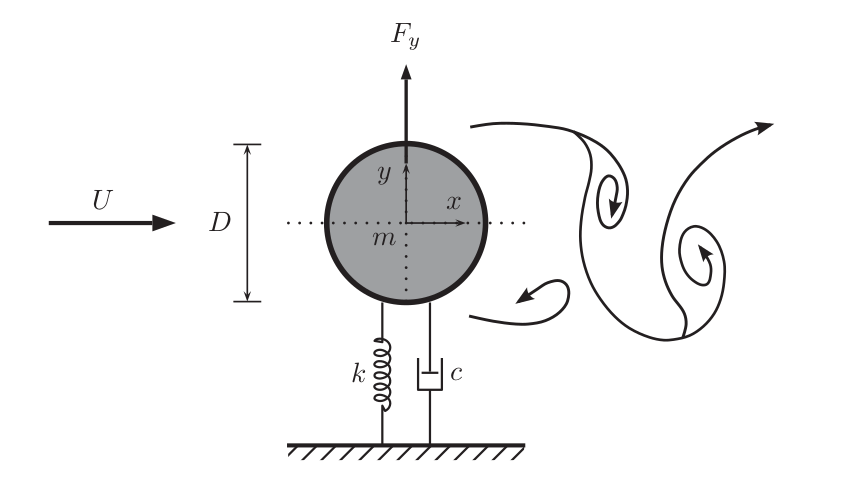
Figure 1: Cross flow vortex-induced vibrations

4.1 Description of the configuration and boundary conditions

Figure 2 depicts the 2D computational grid domain used, which also reports the boundary conditions imposed in the simulations. All the lengths reported are referred to as the problem characteristic length, which is the diameter of cylinder D = $1.0\text{\,}\mathrm{m}$. The grid features is 11 644 cells (control volumes) and 24 440 points, while the physical viscosity $\nu=$0.005\text{\,}\mathrm{k}\mathrm{g}\mathrm{/}{\mathrm{m}\mathrm{s}}$$. Uniform and constant horizontal velocities $\bm{U}_{\infty}=(U_{in},0)$ with $U_{in}=$1.0\text{\,}\mathrm{m}\text{\,}{\mathrm{s}}^{-1}$$ were imposed at the inlet boundary. This corresponds to a Reynolds number of 200. In OpenFOAM [19], the standard boundary conditions allowable are zero-gradient, fixed value, symmetry boundary condition, and moving-wall-velocity. In the simulations, we deal with three types of boundary conditions, namely: inflow ($\Gamma_{in}$), outflow ($\Gamma_{out}$), and solid wall ($\Gamma_{sw}$) as shown in Figure 2.

Figure 2: The OpenFOAM mesh used in the simulations for the unsteady case of the flow around a circular cylinder.

4.1.1 Non-linear solver of the fluid

The simulations are carried out using the non-steady solver pimpleFoam, which is based on merging the SIMPLE and PISO algorithms described in Subsection 3.1. The PimpleFoam solver in OpenFOAM has the capacity to adapt the time steps in a way that assures that the maximum Courant number CFL does not exceed a prescribed value which is, in this case, has been set to $CFL_{max}=0.9$ In the relation of time advancing schemes used in this case, the Euler scheme is used for the computation of the time derivative of the velocity field. As for the spatial gradients, a Gauss linear scheme is employed. The convective term has been approximated with the Van Leer limiter scheme [49]. Gauss linear scheme is used for the discretization of the diffusive term. The values of the relaxation factors $\alpha_{u}$ and $\alpha_{p}$ are fixed at 0.7 and 0.3, respectively. Only one non-orthogonal corrector iteration is used to deal with the mesh’s non-orthogonality. In addition, one correction pressure and three momentum correction are used in the simulations. As for the linear solvers, a smoother Gauss-Seidel solver is used for solving the pressure equation.

4.1.2 Structural solver

The second-order differential Equation 1 is solved using the Symplectic 2nd-order explicit time-integrator for solid-body motion [8]. An Arbitrary Lagrangian-Eulerian (ALE) method is used to deal with the moving mesh resulting from the fluid-structure coupling, where the displacement y and the velocity $\dot{y}=\dfrac{dy}{dt}$ of the cylinder are used to deform the mesh and update the flow velocities respectively. The non-dimensional flow and structure parameters are listed in Table 1 where $U^{*}=\frac{U_{\infty}}{f_{n}D}$ is the non-dimensional reduced velocity. The structural non-dimensional frequency $f_{n}^{*}=\frac{f_{n}D}{U_{\infty}}$, with $f_{n}$ satisfying $\omega_{n}=\sqrt{\dfrac{k}{m}}=2\pi f_{n}$ which leads to $f_{n}^{*}=\frac{1}{U^{*}}$ at the far field. We select a high damping ratio value to control the cylinder oscillations’ amplitude. The flow passes a cylinder for Reynolds number $Re=200$ resulting in the Strouhal number, $St=\frac{f_{sh}D}{U_{\infty}}\approx 0.2$( during the synchronization (lock-in) see Figure 11), where $f_{sh}$ is the frequency of vortex shedding frequency. The Strouhal frequency can be defined as the lift coefficient frequency or the fluctuation frequency of velocity for any point in the near wake. The non-dimensional cylinder frequency $f_{n}^{*}=0.185.$ An explicit expression of the Strouhal number as a function of Re (Reynolds number) can be given as $St=-0.0065\ln{Re}+0.21$ [38]. This means that the Strouhal number decreases as the Reynolds number increases.

Re	$f_{n}^{*}$	$U^{*}$	c (%)	k	m (kg)
200	0.185	5.405	40	0.135114884	0.1

Table 1: Simulation parameters

4.2 Results and discussion

This subsection presents the results of applying POD-Galerkin of a laminar vortex-induced vibration response at Re = 200. The Finite Volume Method (FVM) C++ library OpenFOAM [19] is used as the numerical solver at the full-order level; such a solver is widely used in industrial applications. One advantage of the FVM is that the equations are written in a conservative form, so the conservation law is enforced locally. At the reduced-order level, the reduction and resolution of the reduced order system are carried out using the C++-based library ITHACA-FV (In real Time Highly Advanced Computational Applications for Finite Volumes) [45, 44] developed in a Finite Volume environment based on OpenFOAM. The results generated by applying POD-RBF on the pointDisplacement field parametrized by the center of mass displacement are presented. The interpolation using the RBF in this work has been carried out using the C++ library SPLINTER [12]. A comparison of the response parameters (the lift and drag forces, cylinder displacement, and phase portraits) obtained from OpenFOAM and ITHACA-FV is portrayed. The non-homogeneous Dirichlet boundary condition at the inlet is enforced with the lifting method [47]. Figure 3 depicts the decay of the cumulative eigenvalues corresponding to the three correlation matrices. The energetic optimality of the POD basis functions suggests that only a minimal number of POD modes may be necessary to describe efficiently any flow realizations of the input data, i.e., $N_{Gal}\ll N_{POD}$ In practice, $N_{Gal}$ is usually determined as the smallest integer $M$ such that the Relative Information Content, $RIC(M)=\sum_{i=1}^{M}\lambda_{i}/\sum_{i=1}^{N_{POD}}\lambda_{i}$ is greater than a predefined percentage of energy $\delta=99.9\%$ in this work. It can be observed that the system energy $\geq\delta$ is concentrated in the first 1 POD mode for the pointDisplacement field. This observation implies that the ALE field can be reduced with just $k=1$ POD mode instead of 24 440 grid nodes. One reason for this observation is that the majority of the variance of the pointDisplacement is concentrated at the moving interface and propagates linearly to the far-field boundaries. Thus, with 1-mode, the full-order mesh can be reconstructed within a maximum absolute error less than $0.05\%$, see Figure 7. The POD modes have been obtained by applying POD analysis to snapshot matrices of velocity and pressure fields using 30 modes see Figure 9 and Figure 10.

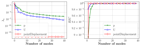
Figure 3: Distribution of modal energy for a laminar flow past a freely vibrating circular cylinder. From left to right, the eigenvalues decay and cumulative eigenvalues of the POD modes. The dashed blue line refers to the velocity eigenvalues, the dashed black line indicates the pressure eigenvalues, and the dashed red line finally refers to the pointDisplacement eigenvalues.

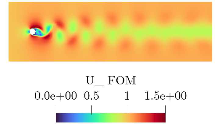
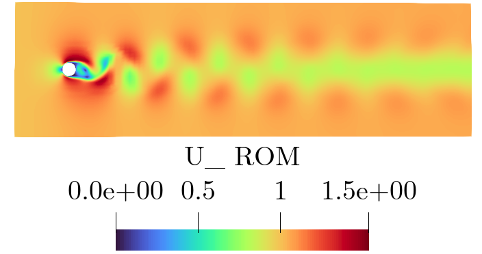
Figure 4: Vortex shedding modes inside the lock-in zone. FOM and ROM velocity solutions from left to right, respectively, at t = 190s.

The main objective of this numerical test is to build a reduced-order model (ROM) which can successfully reproduce the flow fields corresponding to the final periodic regime solution. Figure 4 and Figure 5 show that the ROM can accurately capture the wake dynamics of the velocity and pressure over time. The full-order model (FOM) simulator was run for enough time to reach a periodic regime. Then it was relaunched for 30 s with a constant simulation time step of $0.01\text{\,}\mathrm{s}$ exporting the solution fields every $0.1\text{\,}\mathrm{s}$. One can see in Figure 4 that the vortices are shed alternately from the upper and lower sides of the cylinder, according to the classical von Kármán streets or 2S mode(for 2 ”single”) vortices. The ROM is able to reproduce the vortex shedding patterns with 30 velocity and pressure modes. Figure 6 depicts the pointDisplacement fields of both FOM and POD-RBF reconstructed with one mode. Figure 7 shows the Frobenius norm of the errors of the pointDisplacement and the effect of the number of modes of velocity and pressure on this error. The above error is computed as follows:

$$\epsilon_{pointDisplacement}=\displaystyle\frac{||{pointDisplacement}_{FOM}-{pointDisplacement}_{POD-RBF}||_{F}}{||{pointDisplacement}_{FOM}||_{F}}\times 100\%$$ (55)

Additionally, Figure 8 shows the POD pointDisplacement coefficients obtained in each simulation by using one mode to reconstruct the pointDisplacement field. One can see how the number of velocities and pressure affect the pointDisplacement field. This is because the presence of the lift force in Equation 1 highly depends on the pressure field.

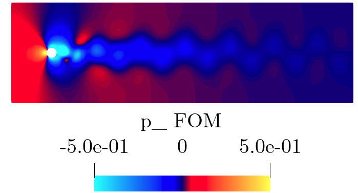
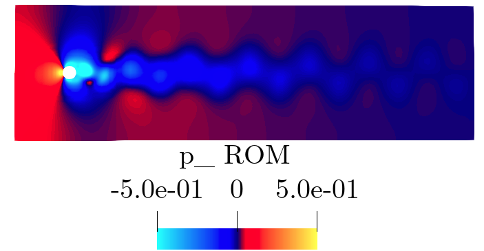
Figure 5: Vortex shedding modes inside the lock-in zone. FOM and ROM pressure solutions from left to right, respectively, at t = 190s.

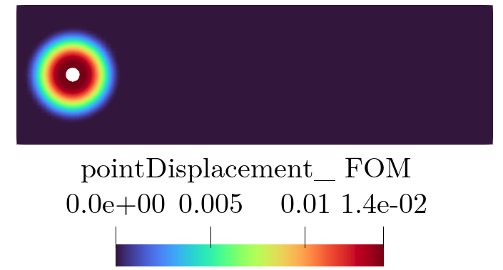
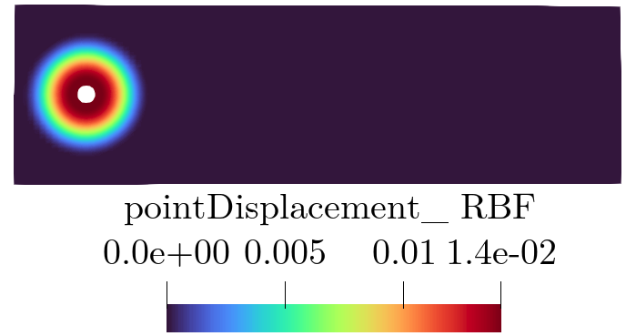
Figure 6: From left to right: FOM and POD-RBF pointDisplacement field solutions respectively at t = 190s.

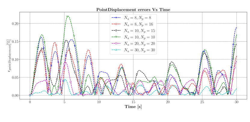
Figure 7: Errors plot of the pointDisplacement fields.

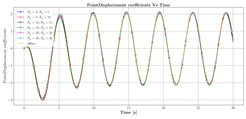
Figure 8: The effect of the number of velocity and pressure modes on the POD pointDisplacement coefficients.

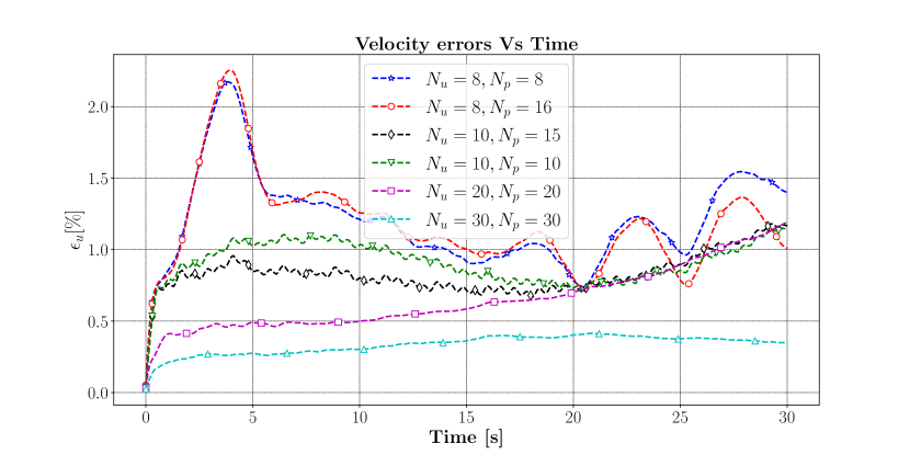
Figure 9: The time evolution of the $L^{2}$ relative errors of the velocity reduced approximation. The error values in both graphs are in percentages.

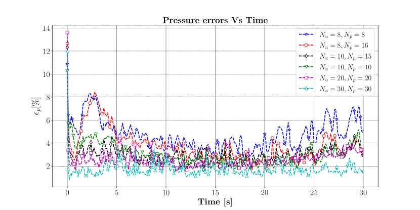
Figure 10: The time evolution of the $L^{2}$ relative errors of the pressure reduced approximation. The error values in both graphs are in percentages.

To provide a quantitative measurement of both models (FOM and ROM) performance, the relative $L^{2}$ error for velocity and pressure are illustrated in Figure 10 and Figure 9, namely:

$$\epsilon_{u}=\displaystyle\frac{||\bm{u}_{FOM}-\bm{u}_{ROM}||_{L^{2}(\Omega)}}{||\bm{u}_{FOM}||_{L^{2}(\Omega)}}\times 100\%\leavevmode\nobreak\ \leavevmode\nobreak\ \leavevmode\nobreak\ \leavevmode\nobreak\ \leavevmode\nobreak\ \leavevmode\nobreak\ \leavevmode\nobreak\ \leavevmode\nobreak\ \leavevmode\nobreak\ \leavevmode\nobreak\ \epsilon_{p}=\displaystyle\frac{||p_{FOM}-p_{ROM}||_{L^{2}(\Omega)}}{||p_{FOM}||_{L^{2}(\Omega)}}\times 100\%$$ (56)

One of the main goals for researchers and engineers studying fluid dynamic problems such as the cross-flow cylinder one here considered is often the evaluation of a force acting on a body or a boundary surface in general. As such forces depend on the local values of the pressure and velocity fields around the body of interest, global error evaluators shown so far (Figure 10 and Figure 9) might not be good indicators if the aim is the assessment on how well the ROM solvers are able to predict the fluid dynamic forces acting on a body. In the case of the present numerical test, for instance, a considerable pressure or velocity error localized in the small region around the cylinder might substantially impact the values of the force while having little effect on the global field errors [14]. For such reason, knowledge of the lift and drag forces acting on the cylinder is essential. As a recall, the expression of the lift and drag forces are given as follows:

$$C_{L} =\frac{1}{\frac{1}{2}\rho U_{\infty}^{2}D}\displaystyle\int_{\Gamma(t)}(\bm{\sigma}_{f}(\bm{x},t)\cdot\bm{n})\cdot\bm{n}_{y}d\Gamma$$ (57)

$$C_{D} =\frac{1}{\frac{1}{2}\rho U_{\infty}^{2}D}\displaystyle\int_{\Gamma(t)}(\bm{\sigma}_{f}(\bm{x},t)\cdot\bm{n})\cdot\bm{n}_{x}d\Gamma$$ (58)

The following analysis considers a side-by-side comparison of the time evolution of the lift and drag forces, displacement of the cylinder, and time series evolution of velocity and pressure coefficients. Figure 11 depicts a comparison of the time-series evolution of the lift and drag forces, respectively, obtained with OpenFOAM and ITHACA-FV. The accuracy of the results is rather satisfactory, especially concerning the values of the Strouhal number and of the lift coefficient, which should be precise as they play a significant role in the study of the VIV.

One of the most exciting characteristics of the fluid body interaction is that of synchronization, or ”lock-in,” between the vortex shedding and the cylinder vibration frequencies. When the wake is synchronized, the vortex-shedding frequency diverges from that corresponding to a fixed cylinder. It becomes equal to the frequency of the cylinder oscillation as shown in Figure 11.

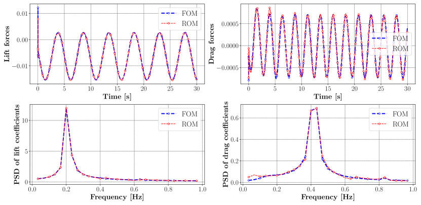
Figure 11: First row: the time histories of the hydrodynamic forces (from left to right the lift and drag forces. Dashed black line is from OpenFOAM, and the dashed red line is from ITHACA-FV) and second row: Power spectra density comparison of the lift and drag coefficients( from left to right respectively. Dashed black line is from OpenFOAM and the dashed red line is from ITHACA-FV)

The periodic state reached is characterized by the oscillation of the drag coefficient at twice ($f_{drag}\approx 2f_{sh}$) the lifting frequency [36] as one can see in the right plot of Figure 11. The time histories of the cylinder displacement are also interesting data because the motion is not known as apriori, as is the case with forced vibrations. The plot in Figure 12 highlights the comparison of the displacement of the center of the mass over time. How accurately the ROM reproduces the time history of the cylinder motion given by OpenFOAM can be observed.

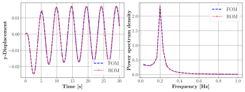
Figure 12: Time series evolution of the center of mass: Dashed black line is from OpenFOAM, and the dashed red line is from ITHACA-FV.

Moreover, phase portraits are an invaluable tool in studying dynamical systems. This reveals information such as whether an attractor, a repellor, or a limit cycle is present. The phase portrait given in Figure 13 complements the PSDs.

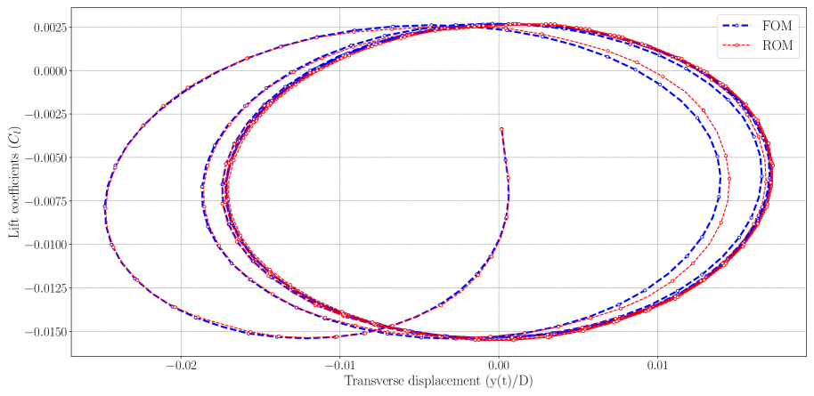
Figure 13: Phase portraits for the cylinder free to oscillate.

It represents the energy transfer (product of the fluctuating lift force characterized by the fluctuating lift coefficient $C_{L}$ and the a-dimensional cylinder displacement $y^{*}=y(t)/D$ between the motion of the cylinder and the fluid and thus provides an interesting description of how the system behaves. The existence of a unique limit cycle results from the perfect damped sinusoidal response, and the inclination of the cycle gives an estimation of the phase angle between the imposed displacement and the lift. It can be seen that the ROM captures the corresponding limit cycle present at the full-order level. In implementing the POD for low-dimensional modeling, we project the governing infinite dimensional evolution equation, such as the NS equations, onto a finite-dimensional empirical sub-space, of possibly quite low dimension. One natural question arises: How well do this truncation and projection approximate the attractor of the original dynamical system? [15]. Figure 15 and Figure 14 give an answer to this question. The ROM accurately reproduces the full-order model’s phase portraits with just 30 modes for both pressure and velocity.

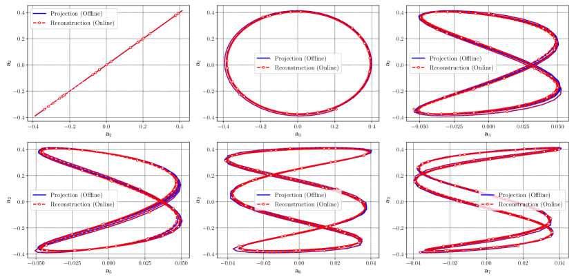
Figure 14: Evolution of the first eight (discard the first coefficient) POD coefficients for velocity obtained from 30 modes with zero initial condition: the blue line is from projection and the dashed red empty cycle from the reconstruction.

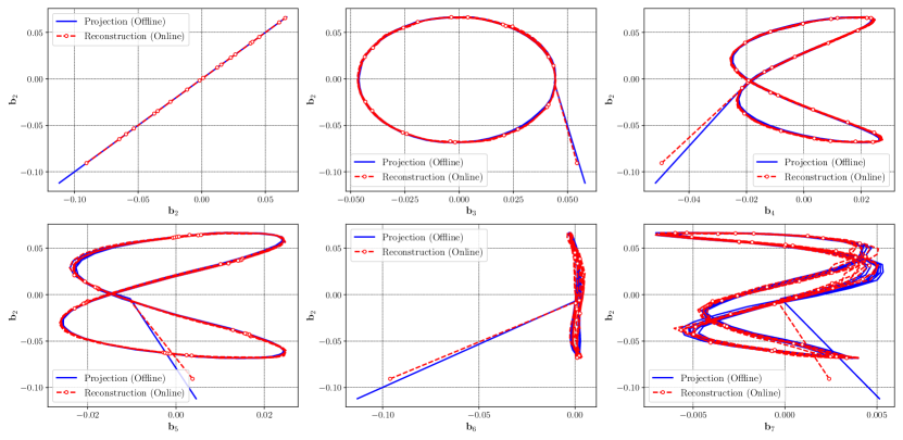
Figure 15: Evolution of the first eight (discard the first coefficient) POD coefficients for pressure reconstructed from 30 modes with zero initial condition: the blue line is from projection and the dashed red empty cycle from the reconstruction.

5 Conclusion and outlooks

This paper presents high-fidelity and surrogate simulations for a flow passing a cylinder with a moving mesh moving boundary in the Arbitrary Lagrangian-Eulerian approach. The computational mesh deformation is considered a part of the solution state vector while constructing the reduced POD basis. The method is demonstrated by using a case study of vortex-induced vibration of a cylinder at a low Reynolds number (Re=200). It has been shown that the design of ROMs for the PIMPLE algorithm with a moving boundary is possible using the ALE approach in the OpenFOAM library framework. This paper proves that the constructed reduced-order model can capture the physics of VIV of a given CFD code based on OpenFOAM solvers and reproduce the specific dynamics of a given laminar regime. It is shown that reduced-order model systems based on POD-ROM have the potential to reproduce changes in dynamics (bifurcations present in the system). The focus of future work will be to apply POD-ROM to flow passing an oscillating cylinder in high Reynolds numbers dependent on a-dimensional parameter-dependent such as mass-damping, rigidity, or reduced velocity.

References

- [1] J. S. Anttonen, P. I. King, and P. S. Beran. Applications of multi-POD to a pitching and plunging airfoil. Mathematical and Computer Modelling, 42(3-4):245–259, 2005.
- [2] J. S. R. Anttonen. Techniques for reduced order modeling of aeroelastic structures with deforming grids. Air Force Institute of Technology, 2001.
- [3] R. A. Ashley. Application of Trained POD-RBF to Interpolation in Heat Transfer and Fluid Mechanics. 2018.
- [4] M. H. Dao. Projection-based reduced order model for simulations of nonlinear flows with multiple moving objects. arXiv preprint arXiv:2106.02338, 2021.
- [5] A. de Boer, M. van der Schoot, and H. Bijl. Mesh deformation based on radial basis function interpolation. Computers & Structures, 85(11-14):784–795, June 2007.
- [6] A. Deane, I. Kevrekidis, G. E. Karniadakis, and S. Orszag. Low-dimensional models for complex geometry flows: application to grooved channels and circular cylinders. Physics of Fluids A: Fluid Dynamics, 3(10):2337–2354, 1991.
- [7] F. Di Donfrancesco, A. Placzek, and J.-C. Chassaing. A POD-DEIM Reduced Order Model with deforming mesh for aeroelastic applications.
- [8] A. Dullweber, B. Leimkuhler, and R. McLachlan. Symplectic splitting methods for rigid body molecular dynamics. The Journal of chemical physics, 107(15):5840–5851, 1997.
- [9] A. Falaize, E. Liberge, and A. Hamdouni. POD-based reduced order model for flows induced by rigid bodies in forced rotation. Journal of Fluids and Structures, 91:102593, Nov. 2019.
- [10] J. H. Ferziger, M. Perić, and R. L. Street. Computational methods for fluid dynamics, volume 3. Springer, 2002.
- [11] L. Garelli. Fluid structure interaction using an arbitrary lagrangian eulerian formulation. CIMEC Document Repository, 2011.
- [12] B. Grimstad et al. SPLINTER: a library for multivariate function approximation with splines. http://github.com/bgrimstad/splinter, 2015. Accessed: 2015-05-16.
- [13] R. Gupta and R. Jaiman. A hybrid partitioned deep learning methodology for moving interface and fluid-structure interaction. Computers & Fluids, 233:105239, 2022.
- [14] S. Hijazi, G. Stabile, A. Mola, and G. Rozza. Data-driven POD-Galerkin reduced order model for turbulent flows. Journal of Computational Physics, 416:109513, 2020.
- [15] P. J. Holmes, J. L. Lumley, G. Berkooz, J. C. Mattingly, and R. W. Wittenberg. Low-dimensional models of coherent structures in turbulence. Physics Reports, 287(4):337–384, Aug. 1997.
- [16] R. I. Issa. Solution of the implicitly discretised fluid flow equations by operator-splitting. Journal of computational physics, 62(1):40–65, 1986.
- [17] A. Ivagnes, G. Stabile, A. Mola, T. Iliescu, and G. Rozza. Hybrid data-driven closure strategies for reduced order modeling. Applied Mathematics and Computation, 448:127920, 2023.
- [18] H. Jasak. Error analysis and estimation for the finite volume method with applications to fluid flows. 1996.
- [19] H. Jasak, A. Jemcov, Z. Tukovic, et al. OpenFOAM: A C++ library for complex physics simulations. In International workshop on coupled methods in numerical dynamics, volume 1000, pages 1–20. IUC Dubrovnik Croatia, 2007.
- [20] H. Jasak and Željko Tuković. Automatic mesh motion for the unstructured finite volume method. Transactions of Famena, 30:1–20, 2007.
- [21] M. C. Kara, T. Stoesser, and R. McSherry. Calculation of fluid–structure interaction: methods, refinements, applications. Proceedings of the Institution of Civil Engineers-Engineering and Computational Mechanics, 168(2):59–78, 2015.
- [22] E. N. Karatzas, G. Stabile, L. Nouveau, G. Scovazzi, and G. Rozza. A reduced basis approach for PDEs on parametrized geometries based on the shifted boundary finite element method and application to a Stokes flow. Computer Methods in Applied Mechanics and Engineering, 347:568–587, 2019.
- [23] E. N. Karatzas, G. Stabile, L. Nouveau, G. Scovazzi, and G. Rozza. A Reduced-Order Shifted Boundary Method for Parametrized incompressible Navier-Stokes equations. Computer Methods in Applied Mechanics and Engineering, 370:113273, 2020.
- [24] K. Kunisch and S. Volkwein. Galerkin proper orthogonal decomposition methods for a general equation in fluid dynamics. SIAM Journal on Numerical Analysis, 40(2):492–515, Jan. 2002.
- [25] E. Liberge, M. Benaouicha, and A. Hamdouni. Proper orthogonal decomposition investigation in fluid structure interaction. European Journal of Computational Mechanics/Revue Européenne de Mécanique Numérique, 16(3-4):401–418, 2007.
- [26] E. Liberge and A. Hamdouni. Reduced order modelling method via proper orthogonal decomposition (POD) for flow around an oscillating cylinder. Journal of fluids and structures, 26(2):292–311, 2010.
- [27] E. Liberge, M. Pomarede, and A. Hamdouni. Reduced-order modelling by pod-multiphase approach for fluid-structure interaction. European Journal of Computational Mechanics/Revue Européenne de Mécanique Numérique, 19(1-3):41–52, 2010.
- [28] M. Mifsud. Reduced-order modelling for high-speed aerial weapon aerodynamics. PhD thesis, 2008.
- [29] T. Miyanawala and R. K. Jaiman. A hybrid data-driven deep learning technique for fluid-structure interaction. In International Conference on Offshore Mechanics and Arctic Engineering, volume 58776, page V002T08A004. American Society of Mechanical Engineers, 2019.
- [30] T. P. Miyanawala and R. K. Jaiman. Decomposition of wake dynamics in fluid–structure interaction via low-dimensional models. Journal of Fluid Mechanics, 867:723–764, 2019.
- [31] F. Moukalled, L. Mangani, M. Darwish, F. Moukalled, L. Mangani, and M. Darwish. The finite volume method. Springer, 2016.
- [32] M. Nonino, F. Ballarin, and G. Rozza. A monolithic and a partitioned, reduced basis method for fluid–structure interaction problems. Fluids, 6(6):229, June 2021.
- [33] S. V. Patankar and D. B. Spalding. A calculation procedure for heat, mass and momentum transfer in three-dimensional parabolic flows. In Numerical prediction of flow, heat transfer, turbulence and combustion, pages 54–73. Elsevier, 1983.
- [34] V. V. Patel. Reduced Order Modeling For Fluid-Structure Interaction Using Machine Learning. PhD thesis, The Ohio State University, 2021.
- [35] A. Placzek, J.-F. Sigrist, and A. Hamdouni. Numerical simulation of vortex shedding past a circular cylinder in a cross-flow at low reynolds number with finite volume-technique: Part 1 — forced oscillations. In Volume 4: Fluid-Structure Interaction. ASMEDC, Jan. 2007.
- [36] A. Placzek, J.-F. Sigrist, and A. Hamdouni. Numerical simulation of an oscillating cylinder in a cross-flow at low Reynolds number: Forced and free oscillations. Computers & Fluids, 38(1):80–100, Jan. 2009.
- [37] I. Prusak, M. Nonino, D. Torlo, F. Ballarin, and G. Rozza. An optimisation-based domain-decomposition reduced order model for the incompressible Navier-Stokes equations, 2022.
- [38] T. L. Resvanis, V. Jhingran, J. K. Vandiver, and S. Liapis. Reynolds number effects on the vortex-induced vibration of flexible marine risers. In International Conference on Offshore Mechanics and Arctic Engineering, volume 44922, pages 751–760. American Society of Mechanical Engineers, 2012.
- [39] C. M. Rhie and W. L. Chow. Numerical study of the turbulent flow past an airfoil with trailing edge separation. AIAA Journal, 21(11):1525–1532, Nov. 1983.
- [40] M. Selim and R. Koomullil. Mesh Deformation Approaches – A Survey. Journal of Physical Mathematics, 7(2), 2016.
- [41] M. M. Selim, R. Koomullil, and D. R. McDaniel. Finite Volume Based Fluid-Structure Interaction Solver. In 58th AIAA/ASCE/AHS/ASC Structures, Structural Dynamics, and Materials Conference, page 0868, 2017.
- [42] S. Shinde and M. Pandey. Modelling fluid structure interaction using one-way coupling and proper orthogonal decomposition (POD). WIT Transactions on Engineering Sciences, 105:27–35, 2016.
- [43] V. Shinde, E. Longatte, F. Baj, Y. Hoarau, and M. Braza. Galerkin-free model reduction for fluid-structure interaction using proper orthogonal decomposition. Journal of Computational Physics, 396:579–595, 2019.
- [44] G. Stabile, S. Hijazi, A. Mola, S. Lorenzi, and G. Rozza. POD-Galerkin reduced order methods for CFD using Finite Volume Discretisation: vortex shedding around a circular cylinder. Communications in Applied and Industrial Mathematics, 8(1):210–236, 2017.
- [45] G. Stabile and G. Rozza. Finite volume POD-Galerkin stabilised reduced order methods for the parametrised incompressible Navier–Stokes equations. Computers & Fluids, 173:273–284, 2018.
- [46] G. Stabile, M. Zancanaro, and G. Rozza. Efficient Geometrical parametrization for finite-volume based reduced order methods. International Journal for Numerical Methods in Engineering, 121(12):2655–2682, 2020.
- [47] S. K. Star, G. Stabile, F. Belloni, G. Rozza, and J. Degroote. A novel iterative penalty method to enforce boundary conditions in Finite Volume POD-Galerkin reduced order models for fluid dynamics problems. Communications in Computational Physics, 30(1):34–66, 2021.
- [48] Y.-Y. Tsui, Y.-C. Huang, C.-L. Huang, and S.-W. Lin. A finite-volume-based approach for dynamic fluid-structure interaction. Numerical Heat Transfer, Part B: Fundamentals, 64(4):326–349, 2013.
- [49] B. Van Leer. Towards the ultimate conservative difference scheme. II. Monotonicity and conservation combined in a second-order scheme. Journal of computational physics, 14(4):361–370, 1974.
- [50] Y. Wang, B. Yu, Z. Cao, W. Zou, and G. Yu. A comparative study of POD interpolation and POD projection methods for fast and accurate prediction of heat transfer problems. International Journal of Heat and Mass Transfer, 55(17-18):4827–4836, 2012.
- [51] M. J. Whisenant and K. Ekici. Galerkin-Free Technique for the Reduced-Order Modeling of Fluid-Structure Interaction via Machine Learning. In AIAA Scitech 2020 Forum, page 1637, 2020.
- [52] D. Xiao, P. Yang, F. Fang, J. Xiang, C. C. Pain, and I. M. Navon. Non-intrusive reduced order modelling of fluid–structure interactions. Computer Methods in Applied Mechanics and Engineering, 303:35–54, 2016.
- [53] B. Xu, H. Gao, M. Wei, and J. Hrynuk. Global POD-Galerkin ROMs for Fluid Flows with Moving Solid Structures. AIAA Journal, pages 1–15, 2021.
- [54] M. Zancanaro, M. Mrosek, G. Stabile, C. Othmer, and G. Rozza. Hybrid neural network reduced order modelling for turbulent flows with geometric parameters. Fluids, 6(8):296, 2021.
- [55] X. Zeng, G. Stabile, E. N. Karatzas, G. Scovazzi, and G. Rozza. Embedded domain Reduced Basis Models for the shallow water hyperbolic equations with the Shifted Boundary Method. Computer Methods in Applied Mechanics and Engineering, 398:115143, 2022.