Constraints on the Initial Mass, Age and Lifetime of Saturn’s Rings from Viscous Evolutions that Include Pollution and Transport due to Micrometeoroid Bombardment

Abstract

The Cassini spacecraft provided key measurements during its more than twelve year mission that constrain the absolute age of Saturn’s rings. These include the extrinsic micrometeoroid flux at Saturn, the volume fraction of non-icy pollutants in the rings, and a measurement of the ring mass. These observations taken together limit the ring {exposure age to be $\lesssim$ a few 100 Myr if the flux was persistent over that time [54]. In addition, Cassini observations during the Grand Finale further indicate the rings are losing mass [50, 87] suggesting the rings are ephemeral as well. In a companion paper [33], we show that the effects of micrometeoroid bombardment and ballistic transport of their impact ejecta can account for these loss rates for reasonable parameter choices. In this paper, we conduct numerical simulations of an evolving ring in a systematic way in order to determine initial conditions that are consistent with these observations.

We begin by revisiting the ancient massive ring scenario of Salmon et al. [79, Icarus 209, 771-785]. Here, we model not just the viscous evolution, but we subject the ring to pollution by micrometeoroid bombardment over the age of the Solar System. We find that regardless of initial mass, the ring always ends up with more pollutant than is currently observed, because the ring spends the majority of its lifetime at relatively low mass where it is most susceptible to darkening. We then show that models with initial disk masses of $\sim 1-3$ Mimas masses reach volume fractions of pollutant consistent with the observed volume fractions of non-icy material in the A and B rings within a time scale of $\sim$ a few 100 Myr.

Finally, we use the analysis of Durisen and Estrada [33] to add the dynamical effects of meteoroid bombardment into the evolution equations, namely, mass loading and ballistic transport. The treatment of mass loading is exact, while ballistic transport is handled in an approximate way. Simulations show that: (1) mass loading and ballistic transport applied to an initially high optical depth annulus inevitably produce a lower density C ring analog interior to the annulus; and (2) high density rings subject to persistent micrometeoroid bombardment do not have an asymptotic mass but instead have an asymptotic lifetime much shorter than the age of the Solar System. This is because micrometeoroid bombardment and ballistic transport drive the dynamical evolution of the ring once viscosity weakens, indicating that the exposure age of the rings and their dynamical age are connected.

1 Introduction

All of the giant planets of the Solar System have ring systems, the majority of which are relatively low mass and composed of ringlets, arcs or gossamer rings and whose photometric characteristics indicate that they are spectrally dark and that water ice is essentially absent or not a dominant compositional constituent [71, 76, 77, 23]. This is in stark contrast to the Saturnian rings which are relatively massive and composed of $>95$% water ice by mass [44, 26, 18, 90, 91]. That Saturn’s rings are so massive and icy is almost certainly a clue to their origin and age. Let us briefly review some current ideas.

1.1 Ring Origin

Several models have been proposed for the origin of Saturn’s rings. Primordial scenarios consider the rings to be unaccreted remnants from the Saturnian subnebula [75], which requires the rings to survive gas drag removal long enough for the subnebula to dissipate. A more recent idea envisions that initially massive rings could have formed from the tidally stripped icy mantle of a Titan-sized differentiated moon at the tail end of satellite accretion [5]. In this model, a Titan-sized, differentiated moon migrates via planetary tides and gas tidal-torques inside Saturn’s Roche limit where its mantle is stripped, while its core is lost to the planet. The rubble disk derived from the mantle forms a new, primarily icy Rhea-sized moon outside the Roche limit (but inside the synchronous radius) that would eventually migrate back inward after the gas disk had mostly dissipated, but still billions of years ago, to be tidally disrupted into a massive ring [see supp. material, 5].

Other ring origin scenarios require sizable interlopers of heliocentric origin. While these events are not all “primordial”, they are usually envisioned to happen billions of years ago and still lead to “ancient” rings. The idea traces back to Harris [46], who suggested that the rings were derived from a previously formed icy moon. The first variant considers the rings to be the remnant of a collisionally disrupted Mimas-mass moon that migrated inward due to gas tidal torque and/or gas drag and was left stranded in a nearly circular orbit near Saturn’s Roche limit when the gas disk dissipated [e.g., 69, 70]. Disruption of this moon probably requires a heliocentric impactor of tens of kilometers in size [7], because Saturn’s tides alone may not be able to disrupt and grind down a cold and solid Mimas-mass moon unless it is very close to the planet [within the C ring, 41, 22]. It has been shown [7] that a Mimas-sized moon located $10^{5}$ km from Saturn can be destroyed with significant probability during the Late Heavy Bombardment (LHB) some 700 Myr after Saturn formed [86]. The key is keeping the moon there long enough for the disruption event to occur. Dubinski [27] recently modeled this scenario in which he assumes that a Mimas-mass body remained close to Saturn because it was trapped in mean motion resonance with Enceladus and Dione.

Another scenario suggests that the rings may be the remnants from a tidally disrupted comet [25, 24]. In this picture, a large ($\gtrsim 200-300$ km) comet or Centaur that passes very close to Saturn may be tidally disrupted with the rings forming from some of the debris. Charnoz et al. [7] also considered this scenario at the LHB and showed that tens of Mimas masses could have been passed through Saturn’s Hill sphere, with a fraction of this material ending up within Saturn’s Roche radius. Although there are caveats [see 7, 6], ideas like these are considered the most plausible “extrinsic” models for ring origin. A significant problem arises, however, for rings that form late in the arc of Solar System history, because the number of suitable interlopers drops off steeply after the LHB [89], making ring formation more and more implausible.

1.2 Ring Age

Although the origin of Saturn’s rings remains unclear, it now seems much more certain when they most likely formed thanks to several key observations provided by the Cassini mission (summarized in Table 1). First, from gravity field measurements in the final orbits of the Cassini Grand Finale, the mass of the rings has been determined to be $\sim 0.4$ Mimas masses [51], lower than the post-Voyager estimate of a Mimas mass [34], but similar to estimates from wavelet-based analyses of several density waves in the B ring [48]. This mass is much lower than what had been envisioned earlier in the mission when it was discovered that the rings had a clump-and-gap structure. Numerical simulations of dense rings had suggested that density waves could hide large amounts of material leading to ring masses an order of magnitude or more than their current mass [84, 78], but apparently this is not the case.

Table 1: Summary of Relevant Cassini Observations

Observation	Instrument	Derived Value
a Flux ($\dot{\sigma}_{\infty}$)	CDA	$2.2\cdot 10^{-16}$ kg m-2 s-1
b Ring Mass	RSS	$(1.54\pm 0.49)\cdot 10^{19}$ kg
c Non-icy Fraction ($\upsilon$)	radiometer	$\sim 1-2$%, C ring/Cassini division
		$\sim 0.1-0.5$%, B and A rings
Mass Inflow	d INMS	$4800-45000$ kg s-1
	e CDA	$\sim 320-1200$ kg s-1
	f MIMI	$\sim 5$ kg s-1

• Kempf et al. [54]

• Iess et al. [51]; Cassini Radio Science Subsystem (RSS)

• Zhang et al. [90, 91]

• Waite et al. [87]

• Hsu et al. [50]

• Mitchell et al. [65]; Magnetospheric Imaging Instrument (MIMI)

Second, Zhang et al. [90, 91], using Cassini radiometer microwave data, showed that the volume fraction of non-icy material in the rings, or “pollutant”, was found to be $\sim 1-2\%$ in the darker, low optical depth C ring and Cassini division and $\sim 0.1-0.5\%$ in the brighter and optically thicker A and B rings. These fractions are consistent with those derived from Voyager observations [26, 18], HST [19] and VIMS results [10], if the pollutant is volumetrically intramixed within the icy grains as tiny inclusions. While visible and IR wavelengths only sample the surface layers of the particles, the microwave measurements sample the bulk of the ring particles, so that the radial variation of pollutants across the rings indeed indicates that the rings overall are not very polluted, and, moreover, have a distinct contrast in the level of pollution between low and high optical depth regions.

Third, observations using the Cassini Cosmic Dust Analyzer (CDA) alleviated the uncertainty about a critical parameter for determining the ring age by measuring the extrinsic micrometeoroid flux at Saturn [54]. CDA found that the flux entering the Hill sphere (which we refer to as “at infinity”) smaller by a factor of two [2, 1, 55, 54] than the previously accepted value [45, 17, 18]. Moreover, orbit reconstruction of the collected impactors shows that the population is consistent with an origin in the Edgeworth-Kuiper belt (EKB) and not the Oort cloud, as previously assumed. Particles from this dynamical population have much lower mean velocities (at infinity) as they enter Saturn’s Hill sphere than cometary particles and thus are about ten times more focused gravitationally by the planet [37]. This implies that the impact flux on the rings is an order of magnitude higher than previously estimated for cometary particles (See Sec. 2.1).

Moreover, measurements during the Cassini Grand Finale orbits, in which the spacecraft flew through the 2000 km region between Saturn’s D ring and the upper atmosphere, revealed that the rings are losing mass at a surprising rate [50, 87, 65]. Some of the mass flux falls as “ring rain” at higher latitudes consistent with the H${}_{3}^{+}$ infrared emission pattern thought to be produced by an influx of charged water products from the rings [73]. However, the contribution needed to account for the ring rain phenomenon is considerably less than the total measured mass influx using the Ion Neutral Mass Spectrometer (INMS) of $4800-45000$ kg s^-1 [87], requiring mechanisms other than the loss of small charged particles to explain. These observations imply that the rings are ephemeral.

Because of their huge surface-area-to-mass ratio, about $\sim 10^{4}-10^{5}$ times more than a moon of equal mass [36], the rings are continuously subjected to bombardment by extrinsic micrometeoroids. This has two main effects. First, micrometeoroid bombardment (MB) can lead to structural evolution of the rings both due to direct deposition of meteoroids and due to the ejecta produced from their impacts with ring particles. The ejecta cause mass and angular momentum transfer because they are often re-absorbed at different locations than where they originate [28, 32], a process referred to as ballistic transport [52]. Durisen and Estrada [33] have recently shown using the CDA measured flux [54] that these effects of MB are large enough to explain mass inflow rates of the magnitude measured by Waite et al. [87]. Second, MB causes icy rings to become more and more darkened with time due to pollution from the non-icy component of the incoming meteoroids [18].

Given these effects of MB, the Cassini measurements taken together constrain the ring age to be $\lesssim$ a few 100 Myr, provided the micrometeoroid flux has been sustained more or less at its currently observed value over that time [54, 33]. The current flux of heliocentric bodies that are large enough to either destroy a resident, differentiated Mimas-mass moon, or to themselves become a ring parent body by tidal disruption, gives a probability of only $\sim 10^{-4}$ for ring formation in the last $\sim 10^{8}$ years [e.g., 63, 53, 25, 7], apparently ruling out such an origin for the rings. So none of the scenarios reviewed in Section 1.1 seem viable, and we currently lack an accepted recent origin scenario [14]. The origin of Saturn’s rings remains an intriguing problem.

1.3 Ring Evolution

The age estimates cited in Section 1.2 are calculated for a static ring and do not take into account ring dynamical evolution. It is important to determine whether age estimates stand up to a proper evolutionary treatment. So this paper reports numerical simulations of a ring evolving under the influence of viscosity and subject to the various effects of MB. Previously, Salmon et al. [79] investigated the global and long-term 1D viscous evolution of an initially massive ring over the age of the Solar System. They used a realistic viscosity model that accounted for enhancement of the viscosity by gravitational instabilities [21]. We employ a similar model here, but we also follow the evolution of the volume fraction of pollutants over time as the ring evolves. We investigate both primordial/ancient ring scenarios and more recent, lower initial mass rings in an effort to determine which are more consistent with the observations. In these first models, we only consider the direct mass deposition (indicated as DD) of the impactors in addition to the pollutant they deliver, and thus these models evolve dynamically solely due to viscosity.

We then add the dynamical effects of mass loading (ML) and ballistic transport (BT) to the numerical evolutions. In this context, by mass loading we mean the mass deposition and the subsequent angular momentum changes that result as a consequence of the impacting meteoroid. Both ML and BT cause an inexorable inward radial drift and thus an influx of ring material toward the central planet. We find that this eventually drives the rings’ dynamical evolution over viscosity for rings whose masses become below a few to several Mimas masses. While ML can be included exactly in the simulations, modeling BT in global simulations is complicated [30, 36, 37] and beyond the scope of this initial study. Instead, we introduce BT approximately in a few of our models by adopting an approach similar to that of Durisen and Estrada [33]. Even though mass is conserved in this approach, it cannot capture the structural changes imposed by BT [e.g., see 36, 37] due to the mass exchanges between different ring regions, which are required for angular momentum conservation. Thus when BT effects are included herein, they should only be considered qualitatively as an indication of the magnitude and direction of its effects, and should be taken with caution. We plan to include BT properly in future work.

This paper is organized as follows. In Section 2, we describe our numerical model by first introducing the basic equations of ballistic transport and deriving the radial drift velocity components. We describe the form of the viscosity law for conditions where the disk is and is not self-gravitating. We also describe the numerical methods including how we follow the evolution of pollutants. In Section 3, we present our simulations. We first model a massive ring under the influence of only viscosity over the age of the Solar System, but include the consequences of pollution by micrometeoroids. We follow this with similar lower mass cases that are evolved over only a few 100 Myr. Finally, we add the dynamical effects of ML (and BT) to the viscous simulations, and show how ML (and BT) profoundly affect ring evolution. In Section 4, we discuss the implications of our findings. Section 5 provides a brief summary of our main conclusions.

2 Ring Evolution Model

In the following sections, we describe the set of equations used to follow the physical and compositional evolution of the rings due to viscosity and micrometeoroid bombardment. Our plan in this paper is to simulate the rings first using viscosity and direct deposition of polluting material only, and later to add the dynamical effects of mass loading and ballistic transport to demonstrate their influence on how fast the rings evolve. A summary of the simulations performed for this work is presented in Table 2.

Table 2: Summary of Simulations

Model type	Eq. solved	$M$(MMimas)	$a$ (m)	$F_{\rm{g}}$	$\eta$ (%)	Figure
V	(7), $\dot{\sigma}_{\rm{im}}=0$	$1-100$	1	…	…	1
DD	(7)	100	1	3	10	3
DD	(7)	100	1	3	$10,100$	4,6a,7a
DD	(7)	100	1	30	$10,100$	5,6b,7b
DD	(7)	$1-100$	1	$3,30$	$10,100$	8
ML	(13), $x{\cal{R}}{\cal{P}}=0$	1	1	30	10	9
ML	(13), $x{\cal{R}}{\cal{P}}=0$	2	1	30	10	10
ML	(13), $x{\cal{R}}{\cal{P}}=0$	3	1	30	10	11
ML	(13), $x{\cal{R}}{\cal{P}}=0$	1	5	30	10	12
ML	(13), $x{\cal{R}}{\cal{P}}=0$	$1-2$	$1-15$	30	10	13
ML[+BT]	(13)	1	1	30	10	14
ML[+BT]	(13)	2	1	30	20	16
ML[+BT]	(13)	$1-1000$	1	30	10	17,18

2.1 Basic Equations

Our approach in this paper is strictly 1D. We only address the radial evolution of ring material and neglect azimuthal and vertical variations. The equation governing the time-variation of the surface mass density $\Sigma$ under the influence of micrometeoroid bombardment and viscosity is given by [37]

$$\frac{\partial\Sigma}{\partial t}+\frac{1}{r}\frac{\partial}{\partial r}\left(r\Sigma v_{\rm{r}}\right)=\Gamma_{\rm{m}}-\Lambda_{\rm{m}}+\dot{\sigma}_{\rm{im}},$$ (1)

where $\Gamma_{\rm{m}}$ is the net gain rate of mass per unit area at some radius $r$ due to absorption of micrometeoroid impact ejecta emitted from other radial locations, $\Lambda_{\rm{m}}$ is the net loss rate of mass per unit area at $r$ due to ejecta emitted at $r$ and absorbed at other radial locations, and $v_{\rm{r}}$ is the total radial velocity of ring material due to viscosity and the effects of MB.

The two-sided micrometeoroid flux $\dot{\sigma}_{\rm{im}}$ that impacts the rings at $r$ is

$$\dot{\sigma}_{\rm{im}}\simeq 2\dot{\sigma}_{\infty}{\mathscr{A}}F_{\rm{g}}(r/r_{0})^{-0.8},$$ (2)

where $\dot{\sigma}_{\infty}$ is the single-sided, flat plate flux entering Saturn’s Hill sphere, $F_{\rm{g}}$ accounts for the gravitational focusing of the micrometeoroid flux by Saturn [17, 18] normalized to a reference radius $r_{0}=1.8$ R_S ($R_{\rm{S}}=60,268$ km is Saturn’s equatorial radius), and the function ${\mathscr{A}}(\tau)=\left[1-e^{-(\tau/\tau_{s})^{p}}\right]^{1/p}$ is a parameterized fit to the numerically determined impact probability [17, 31, 36, 37] as a function of the optical depth $\tau$. The fit parameters are $\tau_{s}=0.515$ and $p=1.0335$ [18]. The $(r/r_{0})^{-0.8}$ factor comes from a fit to the radial dependence of the focusing effect in Cuzzi and Durisen [17]. Most all previous modeling of the effects of MB on the rings [e.g., 30, 18, 36] have assumed the population of impactors are of Oort cloud origin, and adopted the derived value of $\dot{\sigma}_{\infty}=4.5\cdot 10^{-16}$ kg m^-2 s^-1 [see 52, 45, 17, 18]. This population which is isotropic in the heliocentric frame is characterized by a large velocity on entering the Hill sphere so that gravitational focusing is small with the value of $F_{\rm{g}}\approx 3$ [e.g., see 18].

The micrometeoroid flux as measured by Cassini is (see Table 1) $\dot{\sigma}_{\infty}=2.2\cdot 10^{-16}$ kg m^-2 s^-1 [54]. Although in the same ballpark as the previously derived flux, there are important differences. First, the dynamical origin of the population is the EKB (Sec. 1.2), which have isotropic velocities in the frame of the planet. As a consequence their mean velocity when entering the Hill sphere is considerably smaller and $F_{\rm{g}}\approx 30$ [54, see also Morfill et al. 66]. Thus, for a given $\dot{\sigma}_{\infty}$, ten times more mass is hitting the rings with time, and consequently the rings are more susceptible to pollution. Second, it has been previously assumed that the composition of the cometary grains is half water ice. For the EKB population, the volatile component of most grains of the radii detected ($\lesssim 20\mu$m) are not expected to survive their journey to Saturn because the sublimation temperature is reached at 10 AU [67, 43]. So we assume that all of the EKB micrometeoroids are composed of potential pollutant (Sec. 2.4.2). We noted above that the gravitational enhancement by the planet in Eq. (2) is a numerical fit to the radial dependence of the focusing derived from the calculations of Cuzzi and Durisen [17], and is for an Oort cloud population. As pointed out in Durisen and Estrada [33], a more careful treatment for the EKB population should be done along these lines, but the order of magnitude difference in focusing between the two populations remains valid, and has been understood for some time [66].

The continuity equation for the areal angular momentum density can be used to determine an expression for the radial velocity $v_{\rm{r}}$ [36]:

$$\frac{\partial}{\partial t}\left(h_{c}\Sigma\right)+\frac{1}{r}\frac{\partial}{\partial r}\left(rh_{c}\Sigma v_{\rm{r}}\right)=-\frac{1}{2\pi r}\frac{\partial g}{\partial r}+\Gamma_{\rm{h}}-\Lambda_{\rm{h}}+\dot{J}_{\rm{im}}.$$ (3)

Here, $h_{c}=r^{2}\Omega=(GMr)^{1/2}$ is the specific orbital angular momentum for circular motion, $M$ is the central planet mass, and $G$ the gravitational constant. $\Gamma_{\rm{h}}$ and $\Lambda_{\rm{h}}$ are the gain and loss rates of angular momentum per unit area at $r$ due to ejecta gained and lost, $\dot{J}_{\rm{im}}$ is the direct deposition rate of angular momentum per unit area by meteoroids [which is generally small and taken to be zero here; see 31, and below], and $g=-2\pi r^{3}\nu\Sigma(d\Omega/dr)$ is the viscous angular momentum flux in terms of the kinematic viscosity $\nu$. From Equations (1) and (3), one can easily find the radial velocity contributions due to viscosity, ballistic transport, and mass loading (plus associated torques) $v_{\rm{r}}=v_{\rm{r}}^{\rm{visc}}+v_{\rm{r}}^{\rm{ball}}+v_{\rm{r}}^{\rm{load}}$, where

$$v_{\rm{r}}^{\rm{visc}}=-\frac{1}{2\pi r\Sigma}\left[\frac{dh_{c}}{dr}\right]^{-1}\frac{\partial g}{\partial r}=-\frac{3}{r^{1/2}\Sigma}\frac{\partial}{\partial r}\left(r^{1/2}\Sigma\nu\right),$$ (4)

$$v_{\rm{r}}^{\rm{ball}}=\frac{1}{\Sigma}\left[\frac{dh_{c}}{dr}\right]^{-1}\left[\Gamma_{\rm{h}}-\Lambda_{\rm{h}}-h_{c}\left(\Gamma_{\rm{m}}-\Lambda_{\rm{m}}\right)\right],$$ (5)

$$v_{\rm{r}}^{\rm{load}}=\frac{1}{\Sigma}\left[\frac{dh_{c}}{dr}\right]^{-1}\left(\dot{J}_{\rm{im}}-h_{c}\dot{\sigma}_{\rm{im}}\right).$$ (6)

As a first effort to model the simultaneous ring evolution due to viscosity and pollution by extrinsic micrometeoroids, we will ignore those terms in Eq. (1) due to mass loading and ballistic transport and retain only the impact flux (Eq. [2]). As indicated previously, this means that for viscous only evolutions (DD), we will add the mass due to impacting meteoroids, but will ignore the radial drift due to mass loading (Eq. [6]). Treatment of mass inflow due to ML (which includes DD and $v^{\rm{load}}_{\rm{r}}$) will be discussed in a subsequent section. Eq. (1) reduces to the more simplified form

$$\frac{\partial\Sigma}{\partial t}=\frac{3}{r}\frac{\partial}{\partial r}\left[r^{1/2}\frac{\partial}{\partial r}\left(r^{1/2}\Sigma\nu\right)\right]+\dot{\sigma}_{\rm{im}},$$ (7)

for the time evolution of the total surface density, and with the exception of the $\dot{\sigma}_{\rm{im}}$ term is the same as that utilized by Salmon et al. [79] in their simulations. Equation (7) can be solved using a variety of techniques, given a model for the viscosity which we describe next.

2.2 Viscosity Model

The rings are treated as a Keplerian disk with negligible pressure where the viscosity leading to angular momentum transport arises from particle interactions. The various contributions to the viscosity can be divided into a local shear stress component due to particle random motions $\nu_{\rm{L}}$ [42], a non-local component $\nu_{\rm{NL}}$ (also referred to as a collisional viscosity) that comes as a result of the momentum transferred through physical collisions across ring particles [3], and, when the rings are sufficiently dense, a component $\nu_{\rm{grav}}$ due to gravitational scattering in self-gravity wakes [e.g., 80, 20]. The former two components are comparatively weak and only dominate viscous evolution when the ring small-scale transport is not dominated by self-gravity wakes, whereas in a dense, self-gravitating disk, the last component dominates and evolution can be extremely rapid. The gravitational state of the disk is described by the Toomre parameter $Q_{\rm{T}}=c\Omega/3.36G\Sigma$, where $c$ is the radial velocity dispersion of ring particles. The transition from gravitating to non-self gravitating occurs as $Q_{\rm{T}}$ decreases below $\sim 2$ [e.g., 81].

A simple prescription employed in this work [79, for a detailed discussion, see Schmidt et al. 83] is given by

$$\begin{split}\nu=\nu_{\rm{L}}+\nu_{\rm{NL}}+\nu_{\rm{grav}}=\;\;\;\;\;\;\;\;\;\\ \begin{cases}\frac{c^{2}}{2\Omega}\frac{0.46\tau}{1+\tau^{2}}+a^{2}\Omega\tau&\,Q_{\rm{T}}>2;\\ 26\left(r_{h}^{*}\right)^{5}\frac{G^{2}\Sigma^{2}}{\Omega^{3}}+a^{2}\Omega\tau&\,Q_{\rm{T}}\leq 2\\ \end{cases},\end{split}$$ (8)

where $r_{h}^{*}=r_{h}/2a=r(\pi\rho/9M)^{1/3}$ is the ratio of the mutual Hill sphere $r_{h}$ of two identical particles of mass $m$ and density $\rho$ to their mutual radii $a$ [21]. The velocity dispersion $c$ depends on the value of $r_{h}^{*}$: if $r_{h}^{*}\leq 1/2$, the velocity dispersion is regulated by collisions and is $c\sim 2a\Omega$, whereas when $r_{h}^{*}>1/2$ the dispersion velocity is determined by the escape velocity from the particle surface, $c\sim(Gm/a)^{1/2}$ [81, 20, 74]. A slight discontinuity can occur in the transition between the self-gravitating and non-self-gravitating viscosity laws about the value of $Q_{\rm{T}}=2$ in Eq. (8), so we make the choice of using a simple linear smoothing scheme to transition between them over a range of $\Delta Q_{\rm{T}}\pm 0.5$. However, the absence of smoothing does not affect the results.

The viscosity will depend on a variety of ring parameters, the most obvious of which is the mass surface density and its radial variation. Equation (8) is generally applied to an ensemble of same-sized particles, so that the dynamical optical depth $\tau=3\Sigma/4\rho a$. Given the relative simplicity of the the simulations we present herein, we will only explore cases that employ a single particle size and leave more complicated treatments for the future. The viscosity also depends on the porosity $\phi$ of the ring particles through their density, which itself evolves as the rings become more polluted. In this paper, we will model cases in which the ring particles are solid ($\phi=0$), but more generally we will choose $\phi=0.75$ in agreement with fits to ring thermal emission [90, 91].

We recognize that there may be uncertainties associated with adoption of this particular viscosity formulation, but our intention here is to use essentially the same prescription as in Salmon et al. [79] so that our results are directly comparable, and we can better discern effects of the additional physics of pollution, ML, and BT.

2.3 Mass Loading and Ballistic Transport

As discussed above in Sec. 2.1, mass loading (ML) due to micrometeoroid bombardment not only deposits mass and with it pollutant, it also causes radial drifts due to the change it produces in the specific angular momentum of a ring region. These drifts are inward [33].

Furthermore, MB leads to ballistic transport (BT) due to the copious ejecta from impacts that cause exchange of mass and angular momentum between ring regions. Because meteoroid impacts preferentially occur on the leading hemispheres of ring particles, the ejecta from the impacts tend to be prograde and thus decrease the specific orbital angular momentum of a ring region, causing it to drift inwards [32, 30, 29, 17, 36, 37]. This inward drift is derived in detail for a uniform ring evolved under BT alone in Durisen and Estrada [33] using Eqs. (1) and (5). $\Sigma$ stays constant to high order, but $v_{\rm{r}}^{\rm{ball}}$ is negative. The small negative direct mass exchange in Eq. (1) represented by $\Gamma_{\rm{m}}-\Lambda_{\rm{m}}$ is balanced to high-order accuracy by the divergence of the flux term on the LHS of Eq. (1) contributed by the non-zero, negative $v_{\rm{r}}^{\rm{ball}}$.

Thus a direct consequence of micrometeoroid bombardment is that both ML and BT lead to mass inflow in the rings. As shown in Durisen and Estrada [33], this inward transport of material from the B ring to the C ring is probably large enough to account for the mass influx of material observed by Cassini [87, 50].

Inclusion of ML is straightforward. In addition to the nonzero $\dot{\sigma}_{\rm{im}}$ in Eq. (1), we include the radial drift $v_{\rm{r}}^{\rm{load}}$ given by Eq. (6). For this paper, as in Durisen and Estrada [33], we make the simplification in Eq. (6) that the torque due to meteoroid deposition $\dot{J}_{\rm{im}}$ is zero. The actual value of $\dot{J}_{\rm{im}}$ is likely to be negative due to aberration and slant path effects, but the total contribution of angular momentum deposition to radial drift is relatively modest [see, for example, Fig. 1 of 31]. For the viscosity plus ML models discussed in Section 3.3, all the $\Gamma$’s and $\Lambda$’s plus $v_{\rm{r}}^{\rm{ball}}$ are set to zero in the evolution equations.

BT is more complex. The $\Gamma$’s and $\Lambda$’s due to ejecta exchanges are multiple integrals that depend on ejection direction and speed and contain several functions that depend on both $r$ and $\tau$ both at the point of ejection and at the point of absorption [see, for example, 36]. Typical distances over which ejecta are thrown range from 10’s to 1,000’s of kilometers. The multiple integrals increase the expense of calculations and the smaller scales involved are not well represented by our adopted grid-spacing of 78 km (see 2.4.1). Full implementation of BT is left to future work. Instead, we adopt a simplified approach that captures the scale and direction of BT’s effect on global ring evolution.

Durisen and Estrada [33] considered a quasi-steady uniform ring where $\Sigma$ and $\tau$ are constant [see also 32, 36, 37] and simplified the loss and gain integrals using approximations previously made by Lissauer [62] and Durisen [29]. They found that the induced inward radial drift due to ballistic transport (Eq. [5]) can be expressed as

$$\Sigma v_{\rm{r}}^{\rm{ball}}=-2xr{\cal{R}}{\cal{P}},$$ (9)

where $x=v_{\rm{ej}}/v_{\rm{K}}$ is the ratio of ejecta velocity $v_{\rm{ej}}$ to the local orbital speed $v_{\rm{K}}$. ${\cal{R}}$ and ${\cal{P}}$ are the $\tau$-dependent local ejecta mass emission rate, in units of mass per unit area per unit time, and the ejecta absorption probability. These are given by

$${\cal{R}}={\cal{R}}_{\infty}\left(1-e^{-\tau/\tau_{0}}+\frac{\tau}{\tau_{0}}e^{-\tau/\tau_{0}}\right).$$ (10)

$${\cal{P}}=\frac{1-e^{-\tau/\tau_{p}}}{1-e^{-2\tau/\tau_{p}}};$$ (11)

In the above equations, $\tau_{p}\approx 0.5$ represents a typical slant path through the rings, $\tau_{0}=0.28$ and

$${\cal{R}}_{\infty}=2\dot{\sigma}_{\infty}YF_{\rm{g}}(r/r_{0})^{-0.8}.$$ (12)

The functional form of Eq. (12) was determined originally by Cuzzi and Durisen [17].

It should be noted that $v_{\rm{r}}^{\rm{ball}}$ (similarly for $v_{\rm{r}}^{\rm{load}}$) is asymptotically non-zero as $\tau\rightarrow 0$ with both approaching a finite, but maximally negative value for the drift velocity. That is to say, the fastest inward drifts occur at the lowest $\tau$ [see also, 31, 33]. This can easily be seen, for instance, with $v_{\rm{r}}^{\rm{ball}}$ in Eq. (9). As $\tau\rightarrow 0$, the $\cal{R}$ on the RHS is proportional to $\tau$. For constant opacity, $\tau$ is proportional to $\Sigma$. So, as $\tau\rightarrow 0$, the $\Sigma$ on the RHS is canceled by a $\Sigma$ on the LHS.

The magnitude of BT effects is governed by the parameters in Eq. (12). The CDA results reported by Kempf et al. [54] constrain both $F_{\rm{g}}$ and $\dot{\sigma}_{\infty}$ (Sec. 2.1) with the latter being a factor of two lower than the value $4.5\cdot 10^{-16}$ kg m^-2 s^-1 adopted in Durisen et al. [30] and Estrada et al. [36, 37]. The most uncertain parameter is the ejecta yield $Y$ from a hypervelocity cratering event on a ring particle, defined as the ratio of the ejecta mass to the impactor mass. For the impact speeds expected in Saturn’s rings, $Y$ can typically range from $10^{4}$ for impacts into solid targets, to $10^{6}$ for granular or powdery surfaces. [see 36, and references therein]. For this work, we use a value of $Y=10^{4}$, though structural simulations using full BT indicate values as high as $Y\simeq 10^{5}$ are needed to maintain the inner B ring edge [36, 37]. Thus our choice may be conservative. We refer the reader to Durisen and Estrada [33] for discussion of the uncertainties in $Y$, especially as it may pertain to particle porosity.

With this approximation for $v_{\rm{r}}^{\rm{ball}}$, and including mass loading (Eq. [6]) as well, we can rewrite Eq. (1) as

$$\begin{split}\frac{\partial\Sigma}{\partial t}=\frac{3}{r}\frac{\partial}{\partial r}\left[r^{1/2}\frac{\partial}{\partial r}\left(r^{1/2}\Sigma\nu\right)\right]+\;\;\;\;\;\;\;\;\;\\ \frac{2}{r}\frac{\partial}{\partial r}\left[r^{2}\left(x{\cal{R}}{\cal{P}}+\dot{\sigma}_{\rm{im}}\right)\right]+\dot{\sigma}_{\rm{im}}.\end{split}$$ (13)

Equations (9) and (13) are valid for a single $x$, though ejecta will have a distribution of velocities. We thus choose an average value based on assuming an $x^{-3}$ power-law speed distribution from some lower bound $x_{b}$ to an upper bound $x_{t}\gg x_{b}$, as used in previous models of ballistic transport [30, 36]. The weighted average $x=2x_{b}$, with typically $x_{b}=10^{-4}$ [see 36]. This $x_{b}$ corresponds to an ejecta velocity of $2$ m s^-1 at the current radial location of the inner B ring edge. The upper bound on ejecta velocities for $x_{t}$ are typically up to a few 100 m s^-1 [see 33, for more discussion].

There are aspects of this BT approximation that need to be explained. We have omitted the net loss and gains due to mass exchanges between different ring regions $\Gamma_{\rm{m}}-\Lambda_{\rm{m}}$ (first term on the RHS of Eq. [1]). We cannot meaningfully compute those terms here without treating boundary regions properly and without a much higher grid resolution. On the other hand, the prograde nature of the ejecta must inexorably cause an inward drift of ring material, and this is important to include, even in an approximate way. Using Eq. (9) is similar to using the steady-state accretion disk inflow rate $\dot{M}=3\pi\nu\Sigma$ to estimate the viscous flow in an accretion disk. This is only strictly applicable to a steady-state disk [see, for example, 47] but is useful as a rough estimate for the mass inflow in the non-steady accretion case. In the same spirit, Eq. (9) provides a ballpark of the disk inflow even when a BT-active disk is not in a steady state, but we cannot properly account for the detailed mass restructuring. Setting $\Gamma_{\rm{m}}-\Lambda_{\rm{m}}$ to zero at least ensures mass conservation. But angular momentum is not conserved using Eq. (9) except for the idealized case of a strictly uniform ring. So our treatment of BT, while capturing the magnitude and $\tau$-dependence of the mass influx, is incomplete, and thus results including BT in this paper should be viewed with some caution.

In summary, it should be emphasized that our treatment of ML is physically exact and does conserve mass and angular momentum properly as long as the the external deposition torque $\dot{J}_{\rm{im}}$ is zero. Typically, $\dot{J}_{\rm{im}}<0$ can arise from the asymmetric absorption of micrometeoroids by ring particles or from asymmetric mass loss due to impacts, for example by production of hot vapor [31]. The latter could even influence $v_{\rm{r}}^{\rm{ball}}$. Apart from this external torque issue, ML is not only modeled in a physically precise way, but the parameters that determine its magnitude are much better constrained than for BT. For BT, the treatment we employ here is informative and effectively captures the influence of BT in a approximate way. While the magnitude of BT-induced radial drifts is more uncertain, primarily due to the uncertainty in impact yield $Y$, the drifts are likely to be greater than those induced by ML [33].

2.4 Numerical Methods

2.4.1 General Solution

We solve Eq. (7) using a variable time-step, semi-implicit finite-differencing scheme with source terms which are second-order in space and time. The method is only semi-implicit because viscosity is a complicated function of the surface density and optical depth so that expressing these time-variable expressions in tri-diagonal form is not possible. For this reason, we employ a variable time step that is determined from satisfying a Courant-like stability condition that depends on the viscous diffusion time across a bin, namely

$$\Delta t=0.2\frac{(\Delta r)^{2}}{3\nu_{\rm{max}}},$$ (14)

where $\Delta r$ is the uniform grid spacing and $\nu_{\rm{max}}$ is the maximum value of the viscosity at any location in the grid. This step-size criterion provides satisfactory stability with time steps ranging from a few days (from the initial state) to up to thousands of years at the later stages when the disk viscosity is weak. Our simulations are conducted over the age of the Solar System for massive ring cases, and over several 100 Myr for rings of recent origin.

We follow closely the work of Salmon et al. [79] and set our radial grid size to $N=1001$ bins over a radial domain ranging from $r_{\rm{inner}}=61,000$ km to $r_{\rm{outer}}=139,000$ km so that our grid bin size is $\Delta r=78$ km. The initial annulus of ring material can vary in width. For models in which we make direct comparisons to the results of Salmon et al. [79], we choose their initial annulus width of $\sim 3000$ km centered about $110,000$ km. For our massive disk cases, we choose an initial radial extent that also lies well within the grid, typically from $100,000$ to $120,000$ km. For our less massive, recent ring scenarios, the annuli may be thinner and varied in location. These will be pointed out when discussing the particular models.

Once the ring material reaches the inner and outer boundary, it is (1) assumed to be lost to the planet at the inner boundary and (2) assumed to contribute to the formation of an icy moon when lost at the outer boundary [8]. In either case, the boundary condition is determined by continuation of the mass flux (Neumann boundary condition) across the boundary using ghost points that are extrapolated from the grid values. Since mass is removed, we specifically choose $\Sigma=0$ there.

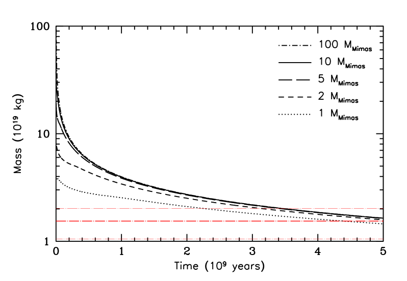
Figure 1: Ring mass as a function of time for different initial masses, which can be compared with Fig. 10 of Salmon et al. [79]. The mass loss for the most massive cases ($M\geq 5$ M_Mimas) occurs very rapidly, indicating that the rings spend most of their lifetime at low mass. As demonstrated by Salmon et al. [79], initially massive rings evolve viscously to an asymptotic mass near the currently observed mass of $1.54\pm 0.49$ kg ($0.41\pm 0.13$ M_Mimas) of the rings [bold dot-dashed red line; 51]. We plot the corresponding error bars given by the bracketing red dot-dashed lines for completeness. There is good agreement between our computational approach and that Salmon et al. [79].

Our solution method differs from Salmon et al. [79], who used a 1D finite elements code on a staggered mesh combined with an explicit, second-order Runge-Kutta scheme. As a test of our code, we reproduce the results from Fig. 10 of Salmon et al. [79] in Figure 1 where we plot the evolution of disk mass over 5 Gyr for initial disk masses of 1, 2, 5, 10 and also for 100 $M_{\rm{\rm Mimas}}$ under viscosity alone (labeled as model V, see Table 2). For these simulations, the mass deposition term $\dot{\sigma}_{\rm{im}}$ is set to zero in Eq. (1) and $v_{r}=v_{\rm{r}}^{\rm{visc}}$ only. We have used a mean particle size $a=1$ m, and the same initial annulus width and starting location ($\sim 3000$ km, centered at $110,000$ km) as in their simulations.

The agreement between the final masses in our evolutions and those in Salmon et al. [79] are within a few percent, while the overall qualitative behavior is the same in both sets of simulations. The disk initially spreads very quickly, especially for a massive ring, filling the domain after which time the ring begins to rapidly lose mass through the boundaries. The most massive case (100 M_Mimas, dash-dotted curve) has already lost 90% of its mass after the first $\sim 10^{7}$ years and is $\sim 3.5$ M_Mimas by $10^{8}$ years. Similar rapid loss rates are observed for the $M\geq 5$ M_Mimas cases, indicating that even in a massive ancient ring scenario, the ring spends the majority of its lifetime at low mass, which has strong implications for rings that are subject to micrometeoroid pollution. We also see that for all of the chosen initial disk masses, the rings viscously evolve to an asymptotic mass as found in Salmon et al. [79] over the age of the Solar System. Like these authors, we see little evolution after 4 Gyr and all ring masses are close to $\sim 1.54\cdot 10^{19}$ kg after 5 Gyr which is their current mass determined by Cassini [bold red dot-dashed line; 51]. The corresponding error bars for their determined mass are given by the bracketing red dot-dashed lines.

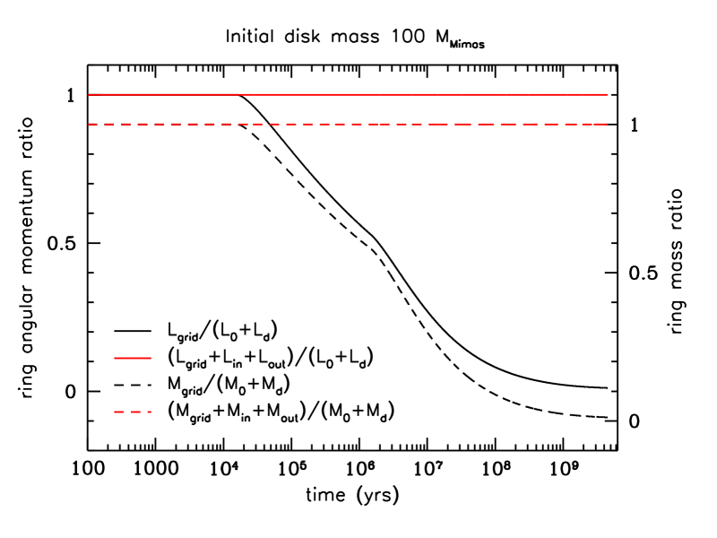
Figure 2: Conservation of mass and angular momentum in a simulation that includes the EKB flux (Sec. 2.4.2) for an initial disk mass of 100 M_Mimas using the same initial conditions as in Fig. 1. Plotted are the evolving ring mass and angular momentum $M_{\rm{grid}}$ and $L_{\rm{grid}}$ (black curves) and their sum with mass and angular momentum lost through the inner and outer boundaries (red curves) in ratio to the total initial and deposited mass and angular momentum associated with micrometeoroid bombardment.

Our numerical code conserves mass and angular momentum well when the ring material evolves only under the influence of viscosity. The total mass and angular momentum of the ring at all times is calculated from summing over all bins

$$M_{\rm{grid}}=2\pi\int_{r_{\rm{inner}}}^{r_{\rm{outer}}}\Sigma r\,dr=2\pi\sum_{i=1}^{N}\Sigma_{i}r_{i}\Delta r,$$ (15)

$$\begin{split}L_{\rm{grid}}=2\pi\int_{r_{\rm{inner}}}^{r_{\rm{outer}}}\Sigma h_{c}r\,dr=\;\;\;\;\;\;\\ 2\pi\sum_{i=1}^{N}\Sigma_{i}\sqrt{GM}r_{i}^{3/2}\Delta r.\end{split}$$ (16)

In Figure 2, we show the conservation of mass and angular momentum for a calculation using Eq. (7) presented in Sec. 2.1 in which the initial disk mass is $100$ M_Mimas, and we include the mass deposition due to the MB but not radial drifts (DD). We plot the ratio of the mass and angular momentum $M_{\rm{grid}},L_{\rm{grid}}$ in the ring (black curves), as well as sums that include the mass (e.g., $M_{\rm{in}}=\sum_{j}\dot{M}_{{\rm{grid}},j}(r_{\rm{inner}})\cdot\Delta t_{j}$) and angular momentum lost through the inner and outer boundaries (red curves), compared to the total (initial + deposited from bombardment), $M_{0}+M_{\rm{d}},L_{0}+L_{\rm{d}}$. The outer edge of the ring encounters the outer boundary of the grid just after $10^{4}$ years, and begins to lose mass rapidly. The inner boundary is encountered after $10^{6}$ years. Despite loss of most of the mass and angular momentum, these losses are well followed over the age of the Solar System, as indicated by the red curves, where we tally the flow of these quantities across the boundaries.

2.4.2 Pollution evolution

The rate per unit area at which a ring annulus of constant surface density $\Sigma$ at some location $r$ is polluted by direct deposition of incoming micrometeoroids is given by Eq. (2). In our code, we incorporate the amount of pollutant that accumulates with time and co-evolve it with the background total surface density $\Sigma=\Sigma_{\rm{pol}}+\Sigma_{\rm{ice}}$, where $\Sigma_{\rm{ice}}$ is the icy material surface density [e.g., see Eqns. 19 and 20 of 37]. Analogous to Eq. (7), the equations for $\Sigma_{\rm{pol}}$ and $\Sigma_{\rm{ice}}$ are

$$\frac{\partial\Sigma_{\rm{pol}}}{\partial t}=\frac{3}{r}\frac{\partial}{\partial r}\left[fr^{1/2}\frac{\partial}{\partial r}\left(r^{1/2}\Sigma\nu\right)\right]+f_{\rm{ext}}\eta\dot{\sigma}_{\rm{im}},$$ (17)

$$\begin{split}\frac{\partial\Sigma_{\rm{ice}}}{\partial t}=\frac{3}{r}\frac{\partial}{\partial r}\left[(1-f)r^{1/2}\frac{\partial}{\partial r}\left(r^{1/2}\Sigma\nu\right)\right]+\\ (1-f_{\rm{ext}}\eta)\dot{\sigma}_{\rm{im}},\end{split}$$ (18)

where $f=\Sigma_{\rm{pol}}/(\Sigma_{\rm{ice}}+\Sigma_{\rm{pol}})$ is the mass fraction of pollutant, $f_{\rm{ext}}$ is the non-icy fraction of the meteoroid and $\eta$ represents the fraction of non-icy pollutant post impact that remains as absorbing material, as assumed in previous ballistic transport modeling [18, 36]. We adopt two values for $f_{\rm{ext}}$: 50%, which corresponds to Oort cloud projectiles, and 100% for EKB projectiles (Sec. 2.1). Equation (13) can be similarly expressed. As the measured values from Cassini for the non-icy material in the rings are given in terms of volume fraction $\upsilon$ [90, 91], we choose to do the same in this paper, so in terms of the mass fraction, $\upsilon=(\rho/\rho_{\rm{pol}})\,f$. We assume the compacted material density of the micrometeoroids $\rho_{\rm{pol}}=2800$ kg m^-3 as is assumed in Kempf et al. [54], which is a mixture of fraction of 70 vol% silicate material, and 30 vol% carbonaceous material [88]. The solid density of a ring particle is then $\rho=\rho_{\rm{pol}}\upsilon+\rho_{\rm{ice}}(1-\upsilon)$ where we take $\rho_{\rm{ice}}=920$ kg m^-3.

At every time step, we calculate the mass fraction $f(r,t)$ from $\Sigma_{\rm{pol}}(r,t)$ and the total mass surface density $\Sigma(r,t)$. The mass fraction of pollutant is then used to calculate the new particle density, and thus the volume fraction $\upsilon(r,t)$, which in turn can affect the optical depth and viscosity at $r$ which must be updated accordingly. It should be noted that because the pollutant is also evolving, this means that an initially icy ring becomes less icy, but as it loses mass at the boundaries, it also loses pollutant. We thus track the total amount of pollutant that impacted the rings and compare it with what remains in the rings as a function of time.

Equation (1) assumes that all of the impactor mass (as given in Eq. [2]) is retained as solid material, but we do not necessarily assume that all of the material remains as a pollutant. We explore two values in our simulations regarding how much of the micrometeoroid retains its radiative absorptive properties after impact: $\eta=10$% and $\eta=100$%. This means that, depending on the choice of $\eta$, as much as 90% of the icy and non-icy components of impactors are assumed to be vaporized and recondensed on the rings, as water ice or as non-absorbing material [26, 18]. We consider the lower value of $\eta$ to be a conservative lower limit because Cuzzi and Estrada [18] found that it was not possible to use lower values and simultaneously explain the relatively sharp contrast in darkening (due to direct deposition) between the low-$\tau$ C ring and high-$\tau$ inner B ring regions, and the much more gradual color transition that arises from the advection of icier (and spectrally more red) material from the B ring to the C ring due to BT across the B-C ring boundary. When allowed to act long enough, BT homogenizes composition regionally, and also globally [independent of $\eta$; 18], but it can also eventually erase the contrast in darkening between the two ring regions, because the more polluted C ring becomes the dominant source of darkening of inner B ring material [36, 37]. On the other hand, too low an $\eta$ may never create a strong darkening contrast because the low-$\tau$ region would be overwhelmed by the advected icy material from the B ring and both regions would darken slowly at more similar rates. So the fact that a relatively sharp darkening contrast exists suggests both a lower limit on $\eta$, and that BT has not acted long enough since the contrast was created to erase it.

Finally, we also consider models in which the micrometeoroid flux was higher in the past. Although this may be a reasonable assumption, pinning an actual value on the flux and how it changes with time is speculative. A factor of ten higher at the LHB may be applicable (K. Zahnle, priv. comm.). Thus for specificity, we consider a model in which the flux is a factor of ten higher up to the LHB ($t_{\rm{LHB}}\sim 700$ Myr), and then let it exponentially decay to its current value as

$$\dot{\sigma}_{\infty}(t)=\dot{\sigma}_{\infty}(t_{\rm{SS}})\cdot 10^{{\rm{MIN}}\left[1,(t_{\rm{SS}}/t-1)t_{\rm{LHB}}/(t_{\rm{SS}}-t_{\rm{LHB}})\right]},$$ (19)

where $t_{\rm{SS}}=4.5$ Gyr.

3 Results

3.1 Long-Term Viscous Evolution of Initially Massive Rings

Let us first consider initially massive rings that are evolving viscously over the age of the Solar System $t_{\rm{SS}}$ while also subject to pollution by micrometeoroid bombardment. We conduct simulations using both the previously assumed Oort cloud (cometary) population and the EKB population because we do not know which may have been dominant over the Solar System lifetime. This means that for the former we choose $\dot{\sigma}_{\infty}=4.5\cdot 10^{-16}$ kg m^-2 s^-1 [45, 17], with a gravitational focusing factor $F_{\rm{g}}\approx 3$, and $\dot{\sigma}_{\infty}=2.2\cdot 10^{-16}$ kg m^-2 s^-1 [54, Sec. 2.4.2] with $F_{\rm{g}}\approx 30$ for the latter. For a few cases, we consider the possibility of a much higher flux during the LHB (Eq. [19]).

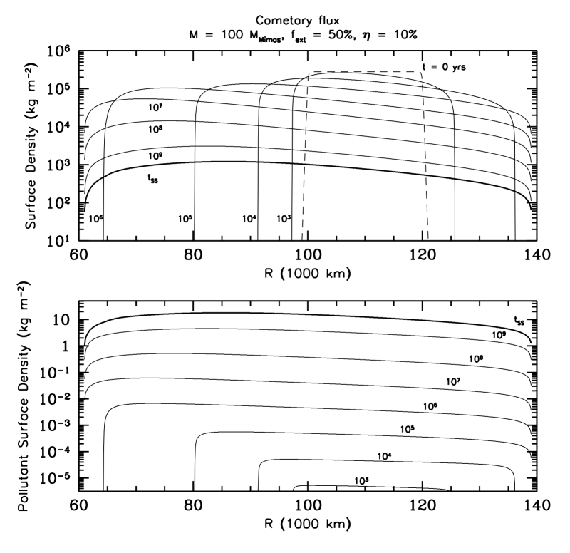
Figure 3: Simulation for an initial 100 M_Mimas ring subject to the cometary micrometeoroid flux for $f_{\rm{ext}}=50$% and $\eta=10$%. upper panel: Surface mass density plotted at various times over the age of the Solar System $t_{\rm{SS}}$. Such a massive ring has already spread to the outer boundary in $\lesssim 10^{5}$ years, while the inner edge is reached after $10^{6}$ years. The ring mass at $t=t_{\rm{SS}}$ is 0.94 M_Mimas. lower panel: Corresponding surface density of accumulated pollutant.

Our fiducial model will be an initial disk mass of 100 M_Mimas ($\sim 1.6\times$ the mass of Rhea), but we will consider the long-term evolution of smaller initial disk masses as well. Naturally, the largest initial disk mass should be the most resistant to pollution. We assume that the ring begins as pure ice. While this seems unlikely, we consider it a conservative assumption that will set an upper limit on the time it takes for the ring to be polluted to what we now observe. Although the current rings are characterized by a particle size distribution with different powerlaw dependencies for different ring regions [e.g, see 19], the viscosity model of Daisaka et al. [21, Sec. 2.2] is derived for a single particle size. We thus adopt a ring particle radius $a$ of one meter, which has been a common choice in $N$-body simulations [e.g., 78, 82], and is also a value similar to the effective radius for ring particles used in BT simulations [e.g., 30, 18, 36].

An initial ring formed from larger chunks will likely grind itself down as it spreads, and thus the size distribution in the rings would change with time affecting the viscosity, but we do not attempt to model this process here. The particle size would directly affect the non-wake viscosity, which increases with particle radius, and the wake viscosity indirectly through the Toomre parameter. Salmon et al. [79] showed that the effect of larger particles is to make the ring evolve more quickly compared to the non-self gravitating regime. We will consider different effective particle sizes for our younger, lower mass ring models in the next subsection.

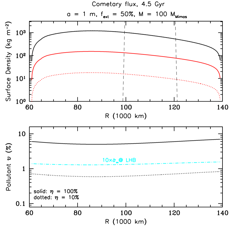
Figure 4: Comparison of simulations for an initial 100 M_Mimas ring at $t=t_{\rm{SS}}$ for the cometary flux with $f_{\rm{ext}}=50$%, and $\eta=10$% and $\eta=100$%. The former corresponds to the case in Fig. 3. upper panel: Final surface mass densities for the $\eta=10$% (dotted curves) and $\eta=100$% (solid curves). The black curves correspond to the total surface density, and the red curves to pollutant surface density. The dashed curve marks the radial extent of the initial annulus. Note that the black curves for the overall surface mass density lie on top of each other. lower panel: Accumulated volume fraction of pollutant for both models. An additional model is included in which the meteoroid influx was higher in the past (Sec. 2.4) for the $\eta=10$% model. The difference leads to about a factor of 2 increase in the non-icy fraction.

Figure 3 shows an evolution of the rings for cometary micrometeoroids with $f_{\rm{ext}}=50$% and $\eta=10$%. We plot the total (ice + pollutant, top panel) and pollutant mass surface densities (bottom panel) for several different times during the simulation. The initial ring annulus is given by the dashed curve. For this configuration, the time for the ring outer edge to reach the outer grid boundary and begin to shed ring mass is $\lesssim 10^{5}$ years, while the inner edge of the grid is reached after $\gtrsim 10^{6}$ years. The characteristic shape of the curves with higher densities inwards are characteristic of a self-gravitating disk. The relative sharpness of the ring edges is mainly due to the viscosity being such a strong function of the surface density. The higher surface density away from edges spreads much more quickly than the lower surface density edge can manage, which further steepens the edge [79]. The bottom panel shows the corresponding surface density of accumulated pollutant. After a time $t_{\rm{SS}}$ (bold curves), the rings have retained a peak value near $10$ kg m^-2 of non-icy material. The final ring mass is 0.94 M_Mimas.

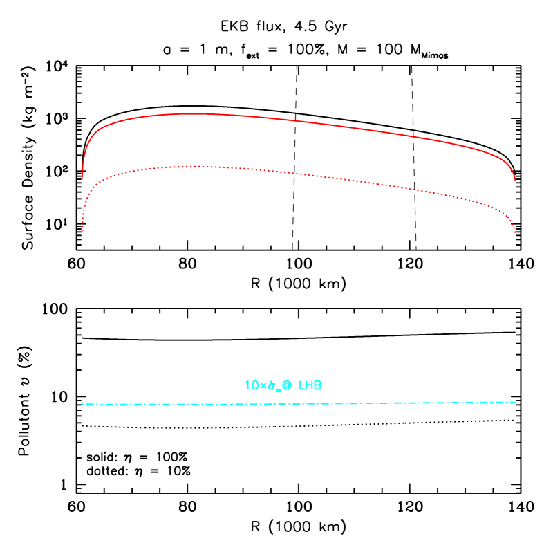
Figure 5: Descriptions are the same as Fig. 4, except that here the EKB meteoroid influx is used, and $f_{\rm{ext}}=100$%. The flux being much higher leads to much darker rings compared to the cometary case, and for the $\eta=100$% model the rings achieve a volume fraction of $\upsilon\sim 50$%. The factor of increase in pollution using a higher meteoroid influx in the past is not as large as it is for the cometary case (see text).

Figure 4 compares the final state of the above simulation (dotted curves) with two additional cases: one where $\eta=100$% (solid curves) and a case where the flux was ten times higher at LHB (dot-dashed, cyan curve) for $\eta=10$%. The dashed curves in the upper panel show the ring edges at $t=0$. The top panel shows the total final surface mass density (black curve) and the final mass densities of pollutants (red curves) for the constant $\dot{\sigma}_{\infty}$ runs. The final total densities curves cannot be distinguished and are generally consistent with surface densities one can infer from the current ring mass [51]. The bottom panel shows the volume fraction of accumulated pollutant. For the conservative case of $\eta=10$%, the pollutant volume fraction is $\sim 0.6-0.7$%, which is consistent with, but slightly larger than current measured values for the A and B rings. The simulation in which the flux is higher in the past and exponentially decays increases the fraction to roughly $1.4$%, or by a factor of two. Thus, an initially massive ring evolving dynamically under viscosity alone for our conservative choice of $\eta$ and the cometary flux apparently allows for ancient rings. The final ring mass is predicted to be larger than the currently observed mass based on the accumulation of micrometeoroids over this time, but the difference in mass is not significant enough to make it inconsistent (also see Fig. 8). On the other hand, the volume fraction for the $\eta=100$% case is nearly ten times larger than measured values, and would be consistent with much younger rings.

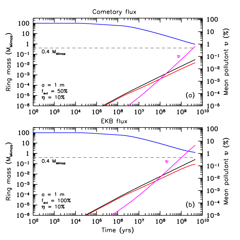
Figure 6: Time evolution of the ring mass (blue curves), accumulated volume fraction of pollutant (mass weighted mean, magenta curves), total mass of pollutant delivered (black curves) and total mass of pollutant retained in the rings (red curves). Compared are the cometary (upper panel) and EKB (lower panel) models show in Figs. 4 and 5 for $\eta=10$%. The dashed line marks the current ring mass. See text for details.

Redoing these simulations for the EKB flux provides a stark contrast, as shown in Figure 5. Now, the $\eta=10$% simulation yields a volume fraction of pollutant of $\sim 4-5$%, or a B ring that has more than ten times the pollution fraction currently observed. The higher flux in the past also increases the level of pollution by slightly less than a factor of two, thus lower than the cometary case, while the $\eta=100$% case produces a volume fraction near 50%, more than a factor of 100 more than currently observed in the B ring.

Figure 6 and Figure 7, for $\eta=10$% and 100%, respectively, summarize the time evolution of the ring mass (blue curves), and accumulated volume fraction of pollutant (magenta curves) for the simulations presented above. The cometary cases are listed in panel (a), and EKB cases in panel (b). The dashed lines indicate the current mass of the rings (Iess et al., 2019). The black solid curves in these figures indicate the total amount of pollutant in Mimas masses that were deposited in the rings, while the red curves are the amount of pollutant that remains in the rings. That is to say, when ring mass is lost at the boundaries, it not only carries away ice, it carries away pollutant with it. The final ring mass for the cometary cases is 0.94 M_Mimas, and 1.23 M_Mimas for the EKB case. The difference in final mass is due to a competition between the amount of mass that has been deposited in the rings versus the more rapid viscous evolution that results from higher surface mass densities. Over the course of the simulation, the rings in the EKB cases have been bombarded by $\gtrsim 2.5$ M_Mimas, but only by $\sim 0.5$ M_Mimas in the cometary case.

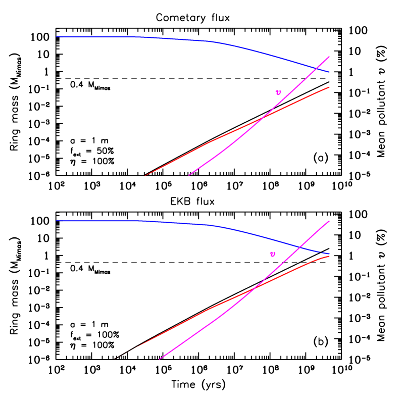
Figure 7: Same descriptions as Fig. 6, except here we compare the cometary (upper panel) and EKB (lower panel) models for $\eta=100$%.

This competition between mass deposition and viscosity is also at the root of the differences seen in the LHB case. Because the meteoroid flux is higher, much more mass is deposited in the rings up to LHB so that the mass of the rings and their level of pollution are higher compared to the nominal constant $\dot{\sigma}_{\infty}$ assumption. The higher mass means that the rings are evolving faster due to higher viscosity and the ring mass drops off more steeply, and with it, more pollutant is removed. The combination of this and a decaying flux eventually closes the gap between the level of pollution in both cases. In the cometary case, the final difference in pollution volume fraction is about a factor of $\gtrsim 2$ (Fig. 4), whereas it is $\sim 1.8$ in the EKB case (Fig. 5). The final masses are smaller, 0.91 M_Mimas and 1.09 M_Mimas for the cometary and EKB cases, respectively.

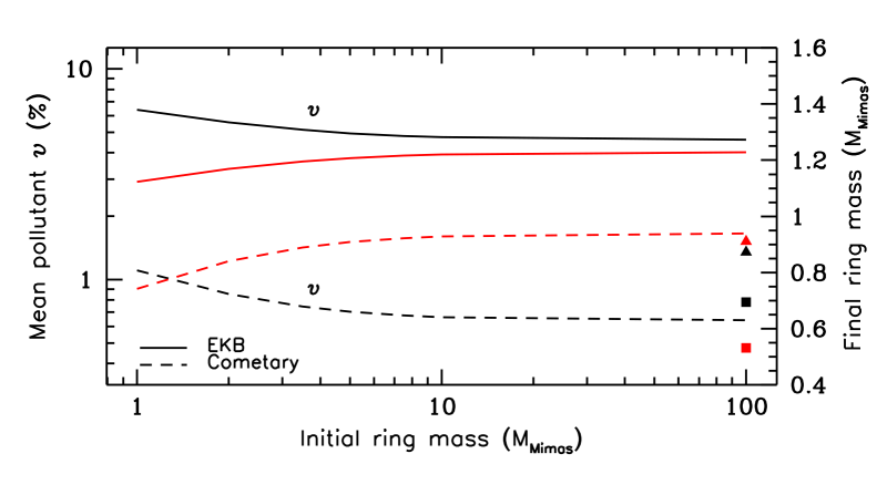
Figure 8: Plot of the overall level of pollutant (black curves), and final ring mass (red curves) as a function of the initial ring mass for a range of models spanning $1-100$ M_Mimas, for $\eta=10$%. The mean level of pollution over the age of the Solar System shows little variation, except at the lowest masses, where rings are darker. The final disk masses also show an asymptotic behavior. Also shown are two additional models for zero porosity (squares), and for the higher flux in the past (triangles).

In Figure 8, we explore the effect of initial disk mass on the overall level of mean pollutant in the rings and on the final ring mass after the age of the Solar System for $\eta=10$% with both cometary (dashed) and EKB (solid curves) fluxes for initial ring masses ranging from 1 to 100 M_Mimas. We find that there is very little difference in the final pollution state of the rings across the full range of initial disk masses (black curves). This is because the rings spend the majority of their lifetime at low mass. For instance, even in the 100 M_Mimas case, the ring mass has dropped due to rapid viscous evolution to $\sim 8-9$ M_Mimas after $10^{8}$ years and to $\sim 2$ M_Mimas after $10^{9}$ years (cf. Fig. 6). The final disk masses (red curves) also show asymptotic behavior with a final preferred ring mass consistent with previous viscous evolution models [79]. The only differences occur for very low initial ring masses where spreading is slower, and the extra time at low mass allows for slightly higher levels of pollutant. We also show results for the higher past LHB flux (triangles) and one with zero porosity (squares), both for 100 M_Mimas and the cometary flux. As noted before, the LHB case leads to a slightly lower final ring mass and rings that are a factor of two darker. The zero porosity case also leads to a much lower final ring mass ($\gtrsim 0.5$ M_Mimas) and is only slightly darker than our nominal $\phi=0.75$ porosity case.

3.2 Short-Term Evolution of Initially Low-Mass Rings

Even in the case of an evolution dominated by cometary meteoroids with $\eta=10\%$, the Solar System age simulations in the previous section give volume fractions of pollutant greater than $0.1-0.5$%. These are larger than what Cassini measurements give in the A and B rings [91], and we know that cometary meteoroids are not dominant at the present time [54]. The final masses of these simulations also do not match the current ring mass [51] even for the smallest initial masses considered due to mass added to the rings from direct deposition over time (see also below), Furthermore, they do not look like the current rings, where the C ring is relatively low mass.

This motivates us to consider simulations starting with lower initial ring masses that are subject to a sustained pollution rate over shorter time periods. In this subsection, and as before, we present models that evolve due to viscosity only (DD), i.e., radial drifts induced by mass loading or ballistic transport are still ignored (Table 2). Because the rings spend the majority of their lifetime at these lower masses, darkening is efficient and should not require long times to reach their current state, even under the assumption that they began as pure water ice.

Based on Cassini CDA measurements of the micrometeoroid flux at Saturn, the implied age of the rings is no more than a few 100 Myr [54, 33]. Moreover, as discussed in Sec. 1, the rings are losing mass at a surprising rate which is attributed in great part to effects caused by micrometeoroid bombardment [50, 87, 73, 33]. Implicit in these mass loss rates is that the rings were more massive in the past. From the results of INMS, which likely measures the total equatorial mass inflow, a constant loss rate would suggest an initial mass for the rings ranging from Mimas to somewhat larger than Enceladus, or from $\sim$ 1 to 3 M_Mimas, some 100’s Myr ago. Adopting this range of initial masses, we will compare the rates of pollution using the recently measured micrometeoroid flux [54] and conservatively assuming a pollutant retention of $\eta=10$%. Our nominal evolutions again assume ring particles with radius $a=1$ m, but we will also explore the effect of particle size on spreading rate (Table 2). Finally, all models presented here begin with a ring annulus from 125,000 km to 130,000 km, but we will later discuss the effects of different initial conditions.

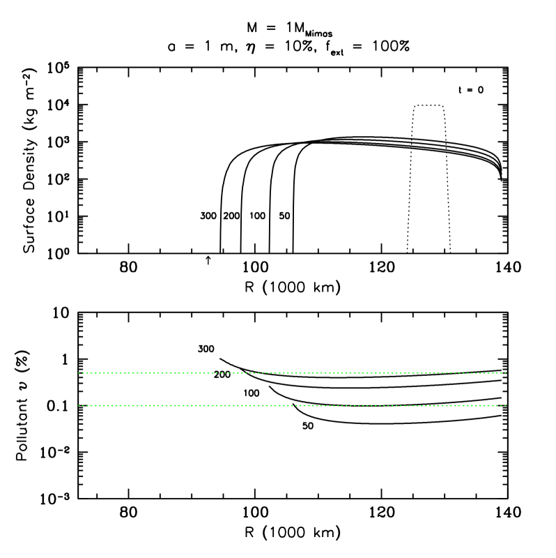
Figure 9: Simulations of an initial 1 M_Mimas ring for $a=1$ m, $f_{\rm{ext}}=100$% and $\eta=10$% for the EKB flux. upper panel: Surface mass density plotted at 50, 100, 200, and 300 Myr. The initial annulus at $t=0$ is shown by the dotted curve. The B-C ring boundary at 92,000 km is indicated by the small arrow. By 300 Myr, the inner edge of the annulus still lies outside the current B-C boundary. lower panel: Evolution of the volume fraction of pollutant at the same times. The 100 and 200 Myr curves bracket the range of observed volume fractions from Cassini for the A and B rings, as shown by the green dotted lines.

Figures 9$-$11 comprise a suite of simulations for initial disk annuli of 1 to 3 M_Mimas . Shown are a set of curves for 50, 100, 200, and 300 Myr. We here assume that, as determined by the CDA analysis [54], the influxing meteoroids are dominated by an EKB population and that this population has dominated at a constant rate over the relatively short duration of these simulations. The top panels plot the ring mass surface density evolution, while the bottom panels give the corresponding level of pollution in the rings. In the former, the dotted black curve shows the ring annulus at $t=0$. In the latter, the dotted green lines mark the range of currently observed non-icy volume fraction in the A and B rings, from $0.1-0.5$% [91].

In the top panel of Fig. 9, which is the lowest initial ring mass model, the spreading naturally occurs at the slowest rate due to the weaker viscosity. The ring encounters the outer edge of the grid and begins to shed mass there after 2 Myr. The disk mass (and masses lost) at 50, 100, 200 and 300 Myr are 0.67 (0.34), 0.62 (0.41), 0.57 (0.48), and 0.56 (0.52) M_Mimas. The amount of mass lost once the outer edge is reached is initially steady, but then begins to decrease with time as viscosity weakens further. The mass that is lost would be relatively icy, and could form its own moon, or contribute to the formation of a moon outside the Roche limit. The retained disk mass at the same time begins to asymptote; however, we expect the disk mass to actually increase at later times because continued direct deposition of incoming material will eventually overwhelm the rate at which viscosity can remove mass from the disk [33] through the outer edge, and, as the disk spreads inwards presenting a larger target for meteoroids, it will continue to accumulate even more mass. We note that in this lowest initial mass case, the inner edge of the annulus has not quite reached the current location of the B-C ring boundary at 92,000 km (marked by the small arrow) even after 300 Myr.

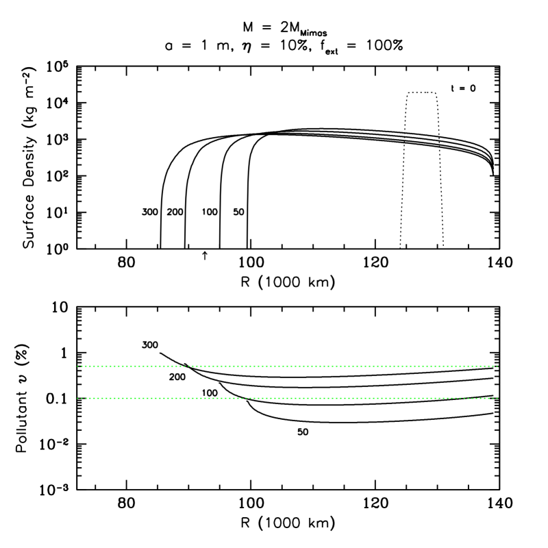
Figure 10: Simulations of an initial 2 M_Mimas ring for $a=1$ m, $f_{\rm{ext}}=100$% and $\eta=10$% for the EKB flux. upper panel: Surface mass density plotted at 50, 100, 200 and 300 Myr. The higher mass ring spreads much further inward, with the 100 Myr case nearly reaching the B-C ring boundary. These simulations shed about a Mimas mass beyond the A ring. lower panel: Evolution of the volume fraction of pollutant at the same times. The 200 and 300 Myr cases bracket the observations, while the 100 Myr marginally does so. Definitions are the same as in Fig. 9.

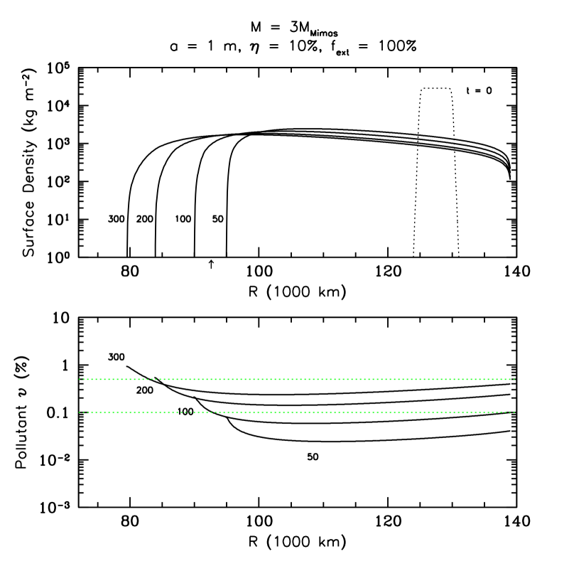
Figure 11: Simulations of an initial 3 M_Mimas ring for $a=1$ m, $f_{\rm{ext}}=100$% and $\eta=10$% for the EKB flux. upper panel: Surface mass density plotted at 50, 100, 200, and 300 Myr. lower panel: Evolution of the volume fraction of pollutant. The 200 and 300 Myr cases continue to bracket the observations, but their inner edges are far inside the B-C boundary. Definitions are the same as in Fig. 9.

The trend of volume fraction of pollutant in the bottom panel of Fig. 9 shows a systematic increase in darkening over time, with the 100 and 200 Myr curves nicely bracketed by the range of observed volume fraction in the A and B rings. Thus, the CDA measured value of the micrometeoroid flux, combined with this conservative choice for $\eta$ would probably be an appropriate fit. The characteristic turn-up of the volume fraction curves shows that lower optical depth regions (at the foot of the inner boundary) are darkening faster. This faster darkening rate is what would be expected to explain the contrast between the A and B ring and the lower optical depth C ring and Cassini division.

For the 2 and 3 M_Mimas mass simulations (Figs. 10 and 11), we see a similar trend in the surface mass density, but the spreading rate is systematically faster with increasing mass due to the higher viscosity, with the B-C boundary location encountered correspondingly sooner. The outer edge of the grid is reached at $\sim 5\cdot 10^{5}$ and $\sim 2\cdot 10^{5}$ yrs, respectively. In the 2 M_Mimas mass case, the disk masses (and masses lost) at 50, 100, 200 and 300 Myr are 1.09 (0.92), 0.99 (1.04), 0.91 (1.15) and 0.89 (1.22) M_Mimas. This model would thus shed about a Mimas mass by itself, but the moon formed would still be mostly ice by mass. The 3 M_Mimas model shows a similar behavior in retained disk mass and mass lost, though the amount of mass lost can be as high as 2 M_Mimas after 200 Myr. As one would expect, these higher mass models show the same behavior of the mass lost beyond the Roche limit decreasing with time, and the retained disk masses are leveling off as is the case in Fig. 9, though it will take more time for the direct deposition rate to eventually exceed the viscous mass loss rate.

In the bottom panels, we note that although there is an overall decrease in the volume fraction of pollutant obtained over these time scales compared with the 1 M_Mimas mass model, the differences are at most about a factor of 2 for the 3 M_Mimas model, so that the CDA measured flux would still satisfy the observed non-icy volume fractions in the A and B rings after $\sim 200-300$ Myrs. These models are conservative in the sense that we use a low value for $\eta$ and the rings are assumed to begin as pure ice. So, a plausible parameter space exists consistent with both very young rings and the current measured level of pollution in the A and B rings where the rings have spread viscously and were polluted by micrometeoroid influx determined by the CDA. Note that a significant feature missing from these evolutions is the development of a C ring structure. Recall, that in these type of models, the inner edge remains sharp because viscosity is such a strong function of the surface density [Sec. 3.1 79]. We will address the formation of C ring structure in Section 3.3 below.

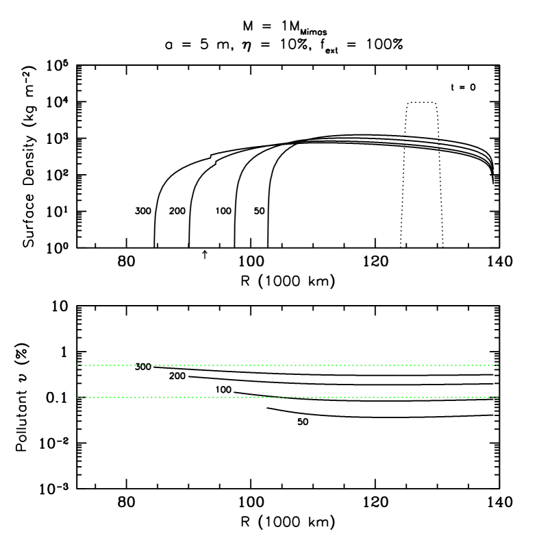
Figure 12: Simulations of an initial 1 M_Mimas ring for $a=5$ m, $f_{\rm{ext}}=100$% and $\eta=10$% for the EKB flux. upper panel: Surface mass density plotted at 50, 100, 200, and 300 Myr. A larger particle size leads to considerably faster evolution, with this case similar to the $a=1$ m, 2 M_Mimas case. The kinks in the curves are due to the ring transitioning from self-gravitating to non-self gravitating forms of viscosity. lower panel: Evolution of the volume fraction of pollutant. Again, similar to the 2 M_Mimas model (Fig. 10), the 200 and 300 Myr cases are bracketed by the observations, but the 100 Myr case only marginally so. Definitions are the same as in Fig. 9.

The initial boundary conditions will have little effect on these outcomes. A ring annulus that begins further inward would encounter the outer boundary at later times, and likely would lose less mass outside the Roche limit, whereas ring annuli that start far enough inward may begin to lose mass to the planet. The amount of mass (and thus pollutant) due to direct deposition that the ring will accumulate will be higher the longer it takes to evolve to a point where ring mass can be lost. The higher ring mass will cause more rapid evolution due to higher viscosity. Regardless of the initial conditions, the darkening rate would be more or less the same as we found for the case of ancient rings (cf. Fig. 8). An apparently robust outcome of these models then is that the level of pollution will reach the observed values over short time scales.

In Figure 12, we show an additional model for a 1 M_Mimas mass in which we choose a ring particle radius of $a=5$ m. As shown by Salmon et al. [79], the immediate effect of using a larger particle size is that the rings spread more quickly. For this choice of $a$, the ring edge reaches the outer boundary only slightly more quickly than the $a=1$ m case at about $\sim 1.9$ Myr. Because of this, slightly more mass is shed from the outer boundary compared to the $a=1$ m case (0.35, 0.43, 0.5, 0.55 M_Mimas for the 50, 100, 200, and 300 Myr curves, respectively).

Although the surface mass densities are considerably lower, the overall spreading behavior for the $a=5$ m case is similar in many respects to the 2 M_Mimas mass case (Fig. 10). In fact, a slight kink is visible near $95,000$ km in the 200 and 300 Myr curves because the ring is transitioning to the non-self gravitating regime. The volume fraction of obtained pollutant (bottom panel) is also more similar and consistent with the 2 M_Mimas model. The lack of a turn up in the volume fraction curves seen in this model compared with the $a=1$ m cases is caused by the overall lower optical depth at the ring edge (1/5 lower for a given surface density), which lowers the probabilities of deposition at the ring inner edge.

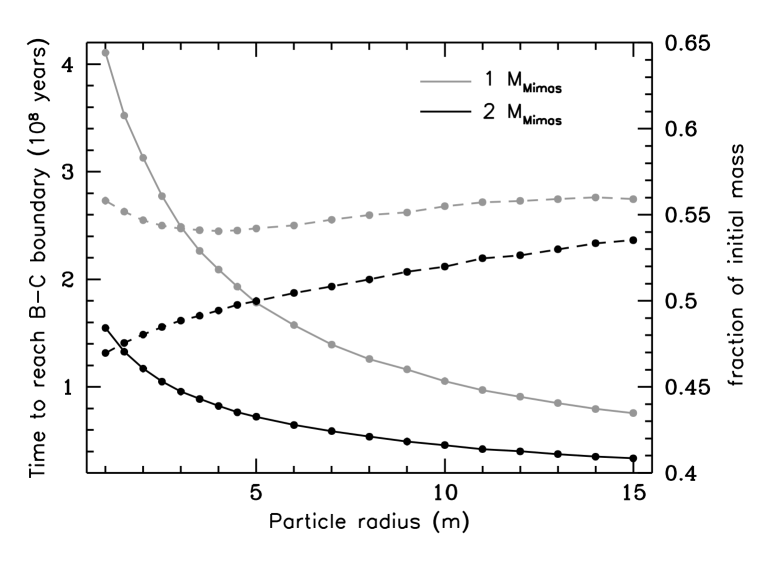
Figure 13: The effects of particle size on the viscous spreading rate for a 1 M_Mimas (grey curves) and 2 M_Mimas (black curves) model. Plotted are the time to spread from the inner annulus boundary at 125,000 km to the location of the B-C ring boundary at 92,000 km (solid curves), and the fraction of the initial mass retained (dashed curves) for particle sizes ranging (indicated by points) from $1-15$ m. The general trend of faster spreading with larger particle size was shown by Salmon et al. [79]. See text.

In Figure 13, we demonstrate the effect of different particle sizes on the viscous evolution of our low mass rings by plotting the time it takes for the ring’s inner edge to reach a reference location, which we take to be the current location of the B-C ring boundary at 92,000 km. Models are shown that correspond to 1 (grey curves) and 2 (black curves) Mimas masses. We also plot the fraction of initial mass left in the ring when the inner edge reaches the B-C boundary (dashed curves). The trends seen further confirm that spreading is much faster as a function of particle size [e.g., see Fig. 13, 79]. At $a\sim 5$ m, though, there appears to be an inflection point where the spreading time for smaller sizes steeply increases, while dropping off gradually for larger sizes. The spreading time to reach the B-C boundary can become quite long, over 400 Myr for the 1 Mimas mass, $a=1$ m case. On the other hand, it takes $\lesssim 100$ Myr when $a=15$ m for the same model. The mass curves generally show a trend of increasing mass retention with increasing particle size. This is simply due to having more time for mass to diffuse outside the Roche limit. However, an uptick is seen for the smallest sizes for the 1 Mimas mass case because spreading is slow enough that the ring has time to acquire a significant amount of mass by direct deposition. The same trend is not seen in the 2 M_Mimas model as of yet because the spreading times to the B-C boundary remain short in comparison even for the smaller particle sizes.

3.3 Effects of Mass Loading and Ballistic Transport on Ring Evolution

In the previous sections, we studied the effects on viscously-evolving rings of the addition of mass and pollutant. In this subsection, we demonstrate the dramatic effect of introducing mass loading (ML) due to direct deposition of bombarding micrometeoroids and a simplified treatment of the dynamical effects of ballistic transport (BT) of impact ejecta on the global evolution of the rings. As discussed in Section 2.3, we are able to compute mass loading exactly but here use an approximation for the inward drift due to ballistic transport that is strictly valid only for a uniform ring. We believe this gives us a correct sense for the direction and magnitude of BT over most of the rings but is inaccurate in the outer regions, over long times, and near edges. For all ML or ML+BT simulations shown in this subsection we assume the EKB population of impactors, and continue to adopt the CDA measured value for the micrometeoroid flux at infinity of $\dot{\sigma}_{\infty}=2.2\cdot 10^{-16}$ kg m^-2 s^-1 (see Table 2).

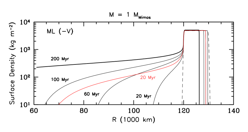
Figure 14: The effect of mass loading (ML), in the absence of viscosity for a 1 M_Mimas initial disk with $\eta=10$%, using the EKB flux (black curves). Curves are plotted at times between $2\cdot 10^{7}-2\cdot 10^{8}$ years. The evolution is characterized by a more rapid flow of material at low optical depths, away from the inner edge of the annulus. A low surface density ring interior to the high surface density annulus is created in a relatively short amount of time. As the material builds up there, the mass influx and loss to the planet becomes substantial. The red curve is a model that includes BT with $Y=10^{4}$ at $2\cdot 10^{7}$ years, which can be compared directly with its ML-only counterpart. The formation of the C ring feature is then much faster due to the much higher induced radial drift.

Figure 14 shows the evolution of a 1 M_Mimas initial mass ring evolving under the effects of ML in the absence of viscosity. The initial conditions are the same as in Section 3.2. The effect of ML is characterized by the flow of material at low surface densities (optical depths) away from the inner edge of the high surface density (optical depth) ring. This inflow is relatively rapid with material reaching the inner edge in $\sim 100$ Myr. Contrast this with the equivalent model in Fig. 13 with only viscosity, where it takes $\gtrsim 400$ Myr (grey solid curve) just to reach the B-C boundary. At first, the mass inflow rate is low, but, as the amount of material builds up in the inwardly extended region, the mass inflow rates from ML become substantial. In the absence of viscosity, the outer edge of the annulus moves inwards. The sharpness of the inner edge appears relatively unchanged because even though the mass flux is high there due to high surface density, the drift velocities are much lower compared with the lower surface density extended region. We show an additional case in Fig. 14 which includes both ML and BT (red curve) plotted at $2\cdot 10^{7}$ years. For BT, we have used the more conservative choice of $Y=10^{4}$. The general effect as expected is even more rapid induced radial drifts compared to ML alone away from the high-surface density inner edge of the annulus.

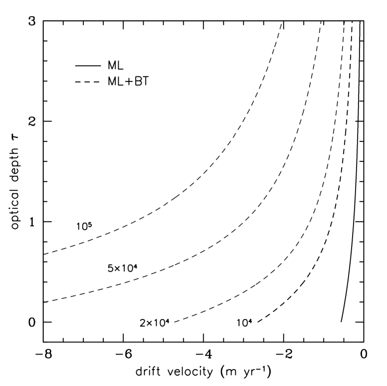
Figure 15: Magnitude of the inward radial drift velocities induced by mass loading (solid curve) and the combination of mass loading and ballistic transport (dashed curves) as a function of the optical depth. Curves for ML+BT are labeled with the value of the impact yield $Y$ assumed for ballistic transport. For reference, the radial location at which these velocities are computed is 120,000 km, the location of the initial inner boundary for the model shown in Fig. 14. The bold dashed curve shows the ML+BT inward drift velocity for our standard choice of $Y=10^{4}$.

This behavior can be better understood by looking at the magnitude of the induced radial drift velocities due to ML and BT. In Figure 15, we show the magnitudes of $v_{\rm{r}}^{\rm{load}}$ and $v_{\rm{r}}^{\rm{load}}+v_{\rm{r}}^{\rm{ball}}$ as a function of the optical depth for the radial location of the inner edge of the annulus of Fig. 14. At high $\tau$, the inward drift velocities are relatively low, but as the optical depth decreases, the drift velocities can increase by over an order of magnitude. For ML, the inward drift of the inner edge occurs because as impacts decrease the specific angular momentum of the material there, it drifts into previously empty regions where impacts at the new radial location decrease its specific angular momentum further, and so on. For BT, owing to the overwhelmingly prograde nature of ejecta, they carry away from their point of ejection more specific angular momentum than is required for a circular orbit there, and arrive at locations further out with less specific angular momentum than needed for a circular orbit [33]. So inward drifts are induced at both locations.

Moreover, the magnitude of the drift velocity for a given $\tau$ increases with decreasing $r$ due to the micrometeoroid impactor focusing by the planet, so for example the ML curve for $2\cdot 10^{7}$ years in Fig. 14 is further along than what the ML drift velocity would predict from Fig. 15 (solid curve) which is the drift velocity at $r=120,000$ km. These drifts become especially severe for BT if large values of the impact yield $Y$ are used in Eq. (12). So, even though the mass influx $2\pi r\Sigma v_{\rm{r}}$ itself may be relatively low, the speed at which ring material drifts inwards is fastest for the lowest optical depths and in fact approaches a limiting value for $\tau\rightarrow 0$ as $2\pi r\Sigma v_{\rm{r}}\rightarrow 0$. This explains why the region inside the annulus is quickly populated with material. The clear implication is that any disk subject to micrometeoroid bombardment will spread inward and lose material faster than by viscosity alone, and that it will continue to do so even when viscosity becomes relatively unimportant. Both ML alone and ML+BT ensure that a radially extended region of lower surface density and optical depth, like the C ring, will form inside an initial dense ring annulus.

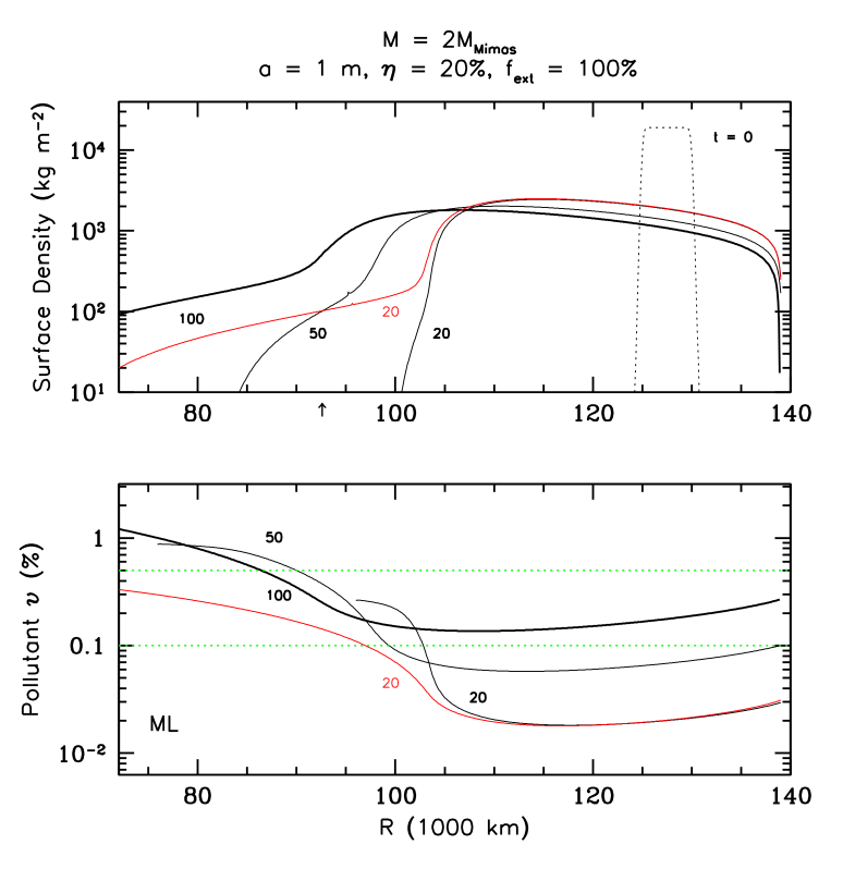
Figure 16: Simulations that includes ML with viscosity (solid curves) for an initial 2 M_Mimas ring with $a=1$ m, $f_{\rm{ext}}=100$%, $\eta=20$% and the EKB flux. upper panel: Surface mass density plotted at 20, 50 and 100 Myr. Like Fig. 14, the formation of a C ring analog occurs relatively rapidly, reaching the location of the inner C ring boundary (75,000 km) at $\sim 70-80$ Myr. The red curve shows the evolution for ML+BT with $Y=10^{4}$ after 20 Myr. lower panel: Evolution of the volume fraction of pollutant. The lower optical C ring analog darkens very quickly in both cases compared to the higher optical depth regions, but eventually becomes diluted as icier material spills in from the denser regions. Even so, after 100 Myr, the volume fraction of pollutant is consistent with observational values. Definitions are the same as in Fig. 9.

In Figure 16, we add viscosity to the effects of ML (black curves) to the evolution of a 2 M_Mimas initial disk (as in Fig. 10), plotted at 20, 50 and 100 Myr. Here we choose $\eta=20$% rather than our nominal $\eta=10$% because of the relatively short time scales involved compared to the model with viscosity only (Table 2). Comparing with Fig. 10, we see that the differences are quite pronounced compared to when only viscosity is included. Strong viscosity in the high surface density regions allows the ring to spread inwards and outwards, but after $\sim 20$ Myr we see a low surface density region forming which spreads to the current location of the inner edge of the C ring ($\sim 75,000$ km) in about $\sim 70-80$ Myr. After 100 Myr, mass is still being lost beyond the outer edge of what would be the A ring. We also include an ML+BT model (red curve) plotted at 20 Myr using $Y=10^{4}$ which shows inward spreading about a factor of $\sim 5$ faster than ML alone. A longer evolution including BT would eventually cause the outer edge of the ring to drift inwards as the magnitude of the induced inflow overwhelms the viscosity. This effect is not entirely realistic because of the approximate nature of our inclusion of BT. When treated properly, we expect the mass inflow will restructure the rings to conserve angular momentum. Until this is done, we cannot say definitively what the behavior at the outer edge will be in the presence of BT [though see Fig. 9.6, 37, also Durisen et al. 32].

The evolution of the volume fraction of pollutant (bottom panel) shows that the contrast between the high and low optical depth regions is strong in both cases. This is well know from earlier pollution evolution studies where the low optical depth regions darken much more quickly than high optical depth regions despite the absorption rates being higher when $\tau$ is large [18, 36, Sec. 2.4.2]. Another well known effect is plainly seen, namely that the radial drift of less polluted material from the higher optical depth regions into the low optical depth regions dilutes it and the volume fraction actually decreases. Comparing the ML curves at 50 and 100 Myr shows that the rings are less polluted in the region between 80,000 and 100,000 km than they were at 20 Myr. This effect would be more pronounced in the ML+BT case. We see that, after 100 Myr, the evolution has reached a non-icy volume fraction in the higher surface density regions that is consistent with the observed values in the B and A rings.

Adding the effects of ML (and BT) indeed appears to form a low surface density (optical depth) region that extends from the inner edge of the high surface density (optical depth) edge to the inner boundary. This idea has been suggested previously [see, for example, 35, 33], but has not until now been explicitly demonstrated. The simulations we conduct here imply that the high-density inner edge, such as the inner B ring edge, would continue to spread and increase the surface density of the lower density C ring. By virtue of the B ring’s less polluted state, this overly dilutes the non-icy material fraction in the C ring. We believe that this is not realistic and is also due to the limitations of our approximate treatment of BT in these simulations which we now explain.

An important effect in full BT simulations, where more than just the BT induced radial drifts are included, is that sharp edges like the inner B ring edge are sculpted and maintained by BT [30, 36]. The B ring inner edge is maintained at its present width through a balance between viscosity and BT because of the prograde-biased ejecta distribution, even as the edge drifts inwards as a unit over longer timescales [59, 61, 37]. The rate of drift of the edge is much slower than the rate at which ring material flows across it. A by-product of this in detailed BT simulations is the formation of a linear ramp of moderate-to-low optical depth that connects the B ring edge to the low optical depth C ring. The ramp is produced by a small excess over direct mass effects of surface density changes caused by differential radial drift when integrated over a power-law ejecta speed distribution [see Section 5a and Appendix B of 30]. When pollution evolution is combined with full BT, we find that the difference in pollution across the edge is sustained for longer times [36] than it is in our current more approximate treatment. Capturing these effects thus requires full BT simulations in which case angular momentum will also be conserved as well.

Clearly, detailed modeling will be required in the future to delineate the formation and maintenance of the C ring at low optical depth. Our current simulations at least suggest that the C ring formed from the B ring and that it can feed mass into the regions close to the planet at a rate regulated by the current mass density in the C ring and by the mass flowing from the B ring into the C ring region. With more detailed BT, we expect that the inner edge of the high-density region in Fig. 16 will remain sharp, and we speculate that this may allow for a mass inflow that achieves some sort of quasi-balance with the B ring inflow. Other effects, not currently included, such as ring rain, may also remove material from near the C ring/inner B ring edge.

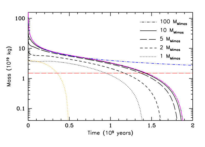
Figure 17: Evolutions of rings with initial disk masses of $1-1000$ M_Mimas under the influence of viscosity and ML. In these simulations, the EKB flux and $\phi=0$ are used. Simulations are stopped when the ring mass reaches $10^{-2}$ M_Mimas. The rings no longer have an asymptotic mass as time increases. Instead, with a given constant meteoroid influx, they have a finite lifetime, which has an asymptotic value as the initial ring mass increases. The 1000 M_Mimas curve, plotted in magenta, lies right on top of the 100 M_Mimas curve and cannot be readily distinguished from it. The red dashed curve indicates the current mass of the rings, and the blue curve is the 100 M_Mimas model when only transport by viscosity is included, as in Fig 1. We show one simulation for an initial mass of 1 M_Mimas (dotted orange curve) where we add BT (with $Y=10^{4}$). This simulation suggests that BT decreases the ring lifetime by a significant factor.

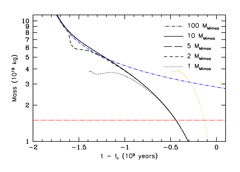
Figure 18: A different visualization of Fig. 17 which demonstrates at what disk mass the rings transition from a viscosity dominated regime to one in which ML dominates. Here we plot time as $t-t_{\rm{f}}$, where $t_{\rm{f}}$ is the time at which the disk mass reaches $10^{-2}$ M_Mimas. The blue curve is as before the viscosity-only 100 Mimas mass case. The ML curves begin to veer away from the latter curve when the disk mass is $\sim 6\cdot 10^{19}$ kg, or roughly 1.6 M_Mimas. Using this format, it is more easily seen that all disk masses eventually follow the same trajectory evolving to smaller masses. The ML+BT case (orange curve) is also plotted which shows that these disk models for a given $Y$ will belong to a different family of curves.

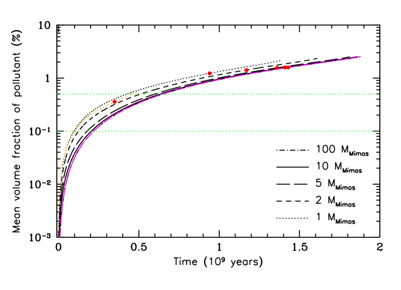
Figure 19: The mean (mass weighted) volume fraction of pollutant as a function of time for initial disk masses from $1-1000$ M_Mimas evolving under the influence of viscosity and ML. In these simulations, the EKB flux, $\phi=0$ and $\eta=10\%$ are used. Simulations are stopped when the ring mass reaches $10^{-2}$ M_Mimas. The green dashed lines mark the observed values of the non-icy volume fractions in the current A and B rings. The red dots indicate where the Saturn’s current ring mass is achieved. By 100 Myr the lowest masses already satisfy the observational constraints, and by 200 Myr all masses do. These simulations indicate that the level of accumulated pollutant is limited by the finite lifetimes. As in Fig. 17, the 1000 M_Mimas (magenta curve) lies on top of the 100 M_Mimas curve. The dotted orange curve corresponds to the 1 M_Mimas case with BT ($Y=10^{4}$) included. The darkening is less due to the faster evolution, but shows that a model with BT can match both the current ring mass and current pollution level constraint simultaneously. Recall that our choice of $\eta$ is conservative. Increasing to 20% would shift these curves upwards by a factor of two.

One result that is strongly suggested by our simulations is that ML and BT will eventually dominate over viscosity in driving the rings’ dynamical evolution. In Figure 17, we plot the evolution of ring mass under the effect of viscosity and ML only for initial disk masses of 1, 2, 5, 10 and 100 M_Mimas (cf. Fig. 1). For these models, we adopt the EKB flux and zero porosity, and have assumed the same initial conditions for the annulus as used by Salmon et al. [79, see Sec. 2.4]. The simulations were halted when the disk mass reached $10^{-2}$ M_Mimas. The black curves show that the rings do not slowly converge asymptotically in mass over long times, as in the viscosity-only cases shown in Fig. 1. For comparison, the blue curve shows the viscosity-only case for 100 M_Mimas. Instead, with ML included, the 100 M_Mimas disk has the longest but still finite lifetime of $\sim 1.88\cdot 10^{9}$ years. The lifetime of the 10 M_Mimas case is only slightly shorter. The lifetime then decreases more rapidly with mass, with the lifetime of the 1 M_Mimas case being $\sim 1.38\cdot 10^{9}$ years. In all cases, the current mass of the rings is achieved sooner than these times. For example, the 1 M_Mimas mass model reaches 0.4 M_Mimas in $\sim 900$ Myr.

Instead of having an asymptotic final mass, we find that the rings have an asymptotic lifetime as the initial ring mass increases. To demonstrate this, the solid magenta curve is for a 1000 M_Mimas initial disk mass which is nearly indistinguishable from the 100 M_Mimas curve. This is not surprising because rapid viscous evolution leads to identical masses for these two cases after only a few million years. Eventually though, the dynamical effects of MB become the leading factor in determining the mass inflow into the planet. Once the rings fall below a threshold mass, their dynamical evolution transitions from a viscosity-dominated regime to one dominated by ML and BT. From Fig. 17, the threshold mass when considering ML alone is $\sim 6\cdot 10^{19}$ kg, or $\sim 1.6$ M_Mimas (which occurs at $\sim 6.7\cdot 10^{8}$ years for for an initial mass $M\gtrsim 100$ M_Mimas). This can be seen more clearly in Figure 18 where we plot the same disk models in terms of $t-t_{\rm{f}}$, where $t_{\rm{f}}$ is the time that the disk reaches $10^{-2}$ M_Mimas.

This result suggests, based on ML alone, that a primordial massive ring would likely have become low mass one much earlier on in Solar System history, especially if the flux was much higher in the past. We have also included an ML+BT model (orange dotted curve) with $Y=10^{4}$ for comparison. Even though the decrease in lifetime (about a factor of three to $\sim 480$ Myr) is consistent with what we might expect, our approximate treatment does not allow us to take this number with confidence. However, it is clear from Figs. 14, 15, and 16 that BT greatly accelerates the evolution in the same sense as ML alone by increasing the radial inward drifts. If the yield is closer to $10^{5}$, the timescale would decrease by another factor of $\sim 5$. Moreover, because BT is even more dominant than ML, the threshold mass below which the effects of MB will dominate the dynamics over viscosity will increase as well.

Figure 19 summarizes the mean volume fraction of pollutant accumulated as a function of time for the ML plus viscosity models shown in Fig. 17. As in previous plots, the green dashed lines mark the range of observed volume fraction of non-icy material in the A and B rings [90, 91]. In these simulations, we have assumed $\eta=10$%. The lowest mass cases begin to satisfy the observational constraints by $\sim 100$ Myr, while all masses satisfy them by $\sim 200$ Myr. By this time, even the largest initial mass models have decreased to $\sim 2.5$ M_Mimas. As in the previous figure, the 1000 M_Mimas case shown by the magenta curve lies right on top of the 100 M_Mimas case. All these curves end as the rings reach $10^{-2}$ M_Mimas, so for each mass there is a similar finite level of pollution achieved ($\lesssim 3$%, though see below). These models with ML alone though are darker than the observed A and B ring non-icy fractions once Saturn’s current ring mass is achieved (red dots). The corresponding case for 1 Mimas mass with BT ($Y=10^{4}$) is shown by the orange dotted curve. The faster evolution further limits the level of pollution compared to ML, but demonstrates that the constraints of Saturn’s current ring mass and the current level of population can be satisfied simultaneously when BT is included. Recall though that we use a very conservative value for $\eta$ which may not be appropriate for impacting micrometeoroids composed primarily of silicates. Increasing $\eta$ can offset the faster evolution; for example increasing to 20% as we did in Fig. 16 would shift the volume fraction curves upwards by roughly a factor of two.

Given these results, the similarity between the current ring mass [51, marked by the red dashed line] and the asymptotic mass derived for ancient rings only subject to viscosity [79] is probably just a coincidence. The asymptotic ring mass simply does not apply to a ring subject to the radial inward drifts caused by micrometeoroid bombardment. The remaining ring lifetime, as derived from measurements of the current mass inflow into Saturn [50, 87, 65, 73] and as estimated from other recent theoretical treatments of mass loading and ballistic transport [33], is generally consistent with the trends as seen in Fig. 17.

4 Discussion

4.1 Simulations with Viscosity and Direct Deposition

4.1.1 Ancient Rings

In our simulations of primordial/ancient rings, we examine two extremes for the amount of pollutant that is retained from an impact, $\eta=10$% and $\eta=100$% and find that, regardless of the initial ring mass, the rings always end up considerably darker than observed for the Cassini measured EKB flux. For the previously assumed cometary flux [45], the current pollution levels could be consistent with the observations only for the $\eta=10$% case. Overall, the volume fractions for the old cometary influx range from $\sim 0.6-6$%, while they are $\sim 5-50$% for the EKB flux for surface densities that would be consistent with the current A and B rings. Since the EKB flux is a measured value, it would appear to rule out a primordial/ancient origin for the rings based on meteoroid deposition of pollutants alone. The amount of pollutant acquired over the age of the Solar System for a given $\eta$ is roughly independent of the initial ring mass, except in the lowest initial mass cases, which acquire more. This is because the rings spend the majority of their lifetime at low masses where they are most susceptible to pollution by MB.

The rings also appear to evolve to an asymptotic mass [as in 79], but this is not surprising since only viscosity is responsible for mass and angular momentum transport in these simulations. Massive rings evolve very quickly to a low mass state due to the high viscosity, and much of the disk mass is removed in short order by losses inwards to the planet or outwards beyond the Roche limit. This lost material also carries away pollutant, with the amount lost typically $\sim 30-50$% of what was delivered over the age of the Solar System. This asymptotic mass is higher than the limit determined by Salmon et al. ($\sim 0.4$ M_Mimas) simply because the rings have accumulated a significant amount of additional mass due to direct deposition over the simulation time (Sec. 3.1). Because of the constant mass deposition rate, eventually over very long time scales the rings will evolve to a state where the mass gained from MB and lost via viscous transport become similar.

We also explore simulations where the flux at LHB was a factor of 10 larger under the reasonable assumption that micrometeoroid flux was higher in the past. The flux is assumed to be ten times higher until LHB and decays exponentially to its current value today. Both for the cometary and EKB flux cases, the level of pollution accumulated is higher, a little more than a factor of two in the cometary case, but a slightly smaller factor of $\sim 1.8$ for EKB. The difference is that much more mass is deposited in the rings up to the LHB, giving them higher surface density compared to the nominal cases, and thus higher viscosity which leads to more rapid evolution. Even though the EKB case gains much more mass, the faster evolution means that the rate of material removal (and thus more pollutant) from the grid compared to the rate of mass deposition (the rate at which they are being polluted) is higher in the EKB case relative to the cometary one.

4.1.2 Young Rings

Our next set of simulations start with a lower initial ring mass and only evolve for a few 100 Myr, now using the observed value for the EKB flux, as given in Kempf et al. [54], in the conservative limit of $\eta=10$%. The mass influx rates of material falling into Saturn from the rings based on Cassini measurements during the last 22 orbits of the Grand Finale [87, 50, 65] imply that the rings were more massive in the recent past. For this reason, we chose to explore models with initial masses of $\sim 1-3$ M_Mimas.

All such simulations produce the observed volume fraction of pollutants in the A and B rings on the time scale of $\sim 100-300$ Myr, with higher masses naturally taking somewhat longer to darken to the same state as lower masses. A higher $\eta$ will make darkening that much easier and would suggest even younger ages for the rings. For the given initial conditions, larger initial mass disks spread further inwards maintaining a relatively sharp edge due to the viscosity being a strong function of $\Sigma$, but do not reach the planet in the simulation times, while models with $\gtrsim 2$ M_Mimas can shed a Mimas mass or more outside the Roche limit to perhaps contribute to the formation of an icy moon. We note that different initial conditions (in the location of the initial annulus) only lead to differences in how much mass is shed, not to the level of pollution.

4.2 Young Rings Including Mass Loading and Ballistic Transport

The inclusion of ML and BT produces radially inward drift velocities that increase both with decreasing optical depth, and with decreasing $r$ because of gravitational focusing of the micrometeoroid flux by the planet. So the material at the lowest optical depths, which occur at the base of the initial ring annulus, drifts inward faster than the material at high optical depth. As a result, ML and, to even greater extent, BT quickly lead to the formation of a low surface density, low optical depth ring interior to the main ring annulus. The drifts are always inwards due to ML because the meteoroid mass decreases the specific orbital angular momentum of the ring material. The drifts are also always inward due to BT because the ejecta from meteoroid impacts are predominantly prograde. Both mechanisms naturally produce a structure resembling the C ring that extends down to the planet, where material is lost to the parent body much more rapidly than by viscosity alone.

Viscous simulations for an initial mass of 2 M_Mimas that include either ML alone or both ML and BT do show much more rapid evolution. The formation of a C ring is a robust feature. We choose a slightly higher $\eta=20$% because of the shorter run times, but the darkening time remains roughly the same. The low optical depth region darkens very quickly relative to the higher optical region, but, as more and more mass fills the C ring region, the ring material becomes diluted by icier material flowing into it from the higher optical depth ring. Both of these effects are basic features of pollution under BT [e.g., see 18]. However, the rapid rate at which bright material flows from high to low optical depth regions in these simulations is exaggerated by the simplified treatment of BT in this paper. Important structural aspects of BT evolution (which incidentally are required for angular momentum conservation), such as maintenance of the B ring inner edge and the formation of the linear ramp at its base [30, 60, 61, 36], are not properly captured by our approximations. Even though material drifts across the edge, the edge itself should maintain a steady sharpness, even as it migrates inward at a reduced pace [59, 37]. We expect that in a full BT simulation, the C ring will still form but the edge between the low and high optical depth regions will stay relatively sharp and not smear out indefinitely in width so that the region interior to it will remain at lower optical depths. This will be the subject of future modeling.

In the viscous evolution of a massive ring, the ring approaches an asymptotic mass over the age of the Solar System independent of its initial mass (see Fig 1; see also Salmon et al. 79). As shown in Fig. 17, our simulations demonstrate that a disk subject to micrometeoroid bombardment no longer has an asymptotic mass at long times, but instead, given a sustained meteoroid influx, has an asymptotic lifetime as the initial ring mass increases. In fact, when ML is included in a viscous evolution, there is no perceivable difference in the lifetime of rings with initial masses of 100 and 1000 M_Mimas, whereas an initial 10 M_Mimas mass disk has a notably shorter lifetime, and the lifetime decreases systematically with decreasing mass. Including BT in addition to ML will undoubtedly make the lifetimes even shorter, up to more than an order of magnitude, depending on the assumed ejecta impact yield $Y$. However, we have less confidence in the quantitative accuracy of this last result because of the simplifying approximations made for BT used in this paper.

4.3 Some Caveats and Speculations

4.3.1 Ring End States

The results of Sec. 3.3 (Fig. 17) indicate that when ring simulations include ML a primordial massive ring may have an asymptotic lifetime much less than the age of the Solar System. Including BT significantly shortens this lifetime. However, all our simulations including ML or BT are idealized in the sense that all material is eventually “lost”. More realistic models which account properly for conservation of angular momentum due to BT will likely leave some material behind in the disk [see, e.g., 32, 37], albeit it at low optical depth/surface density where the effectiveness of mass and angular momentum transport due to ML and BT are lessened. For instance, a thin, low optical depth ringlet may be subject to MB, but the throw distances of ejecta (defined by their velocities) increasingly lie outside the radially thin ring so that the ejecta would return to their point of origin effectively neutralizing BT. Only ML would play a role. External torques due to moons [see 33, for more discussion on this issue], or shepherding of ring annuli by small moonlets might also influence the long term outcome. Moreover, such ringlet systems would be free to continue to darken from meteoroid bombardment beyond the values seen in Fig. 19.

Our results thus lead us to speculate that the eventual “end state” of a massive ring evolving under the combined effects of viscosity, mass loading, and ballistic transport may ultimately resemble something like the ring systems of Uranus and Neptune. This is in agreement with Crida and Charnoz [12] who first posited that these bodies may have initially had massive rings, but then could not explain why these planetary ring systems were well below their asymptotic mass. For instance, a similar calculation for Uranus as those shown in Fig. 1 yields an asymptotic mass of $\sim 0.06$ M_Mimas, or $\sim 2\cdot 10^{18}$ kg, which is more than two orders of magnitude larger than the estimated mass of the Uranian rings [40, 68, 9]. This mystery can apparently be solved, though, if one considers that MB can drive ring dynamics once viscosity is ineffective.

4.3.2 Micrometeoroid Flux

In all of our simulations, we have implicitly assumed that the micrometeoroid flux was constant at its Cassini measured value or was higher in the past. The latter is a reasonable assumption given that there would have been much more source material around up to the LHB [89]. Recall we found only one case, based on viscous evolution only for $\eta=10$% and the cometary flux, in which the rings current level of pollution can be compatible with ancient rings (Sec. 3.1). Given our findings from Sec. 3.3, and our discussion in Sec. 4.3.1, though, this result is not realistic. We cannot say for certain, though, that this has been the case in the more recent past. One could consider that it may be possible that the flux may have been weaker, or inactive for periods over that time potentially allowing for rings that could be considerably older than what our models predict.

We argue that this is unlikely based on a combination of our simulations here, and on detailed ballistic transport calculations which offer an argument in favor of a continuous flux with only minor variation. Simulations show that structural evolution of the rings due to BT requires a roughly constant flux over 100’s to 1000’s of gross erosion times to form and/or maintain observed structures such as the inner B ring edge and the roughly linear ramp that connects the edge to the C ring [36, 37]. The gross erosion time $t_{\rm{G}}=\Sigma/Y\dot{\sigma}_{\rm{im}}$ is the time it would take a ring region to completely erode away if all locally produced ejecta were lost, and none were gained [28]. We can compare this to the pollution time to darken the B ring ($\upsilon\sim 0.3$%) to its current state [see Sec. 2.4.2, 54, 33]

$$\Delta t_{\rm{pol}}\simeq\frac{\rho_{\rm{pol}}}{\rho}\upsilon\frac{Y}{\eta}t_{\rm{G}},$$ (20)

which for our range of $Y$ and $\eta$ gives $\sim 10^{2}-10^{4}$ t_G, in rough agreement with structural times mentioned above.

The structural time for the inner B ring and C ring ramp though are not necessarily the same as the exposure or formation age of the rings. As has been shown previously [59, 61, 37], the relative sharpness of the inner B ring edge can be maintained, even if it migrates inwards as a unit. This implies it would have formed further away from Saturn than its current radial location at $\sim 92,000$ km. It should be noted that micrometeoroid bombardment and BT cannot create the inner B ring edge, only sculpt and maintain it against viscosity [30, 36, 37, Sec. 3.3]. Therefore, an initial relatively sharp inner edge is required which is facilitated in our models because the initial massive ring annulus has a sharp edge due to the viscosity’s strong dependence on surface density (Sec. 2.4.1 and 3.1). We saw that in our simulations as the annulus evolves, a C ring structure is formed emerging from the low optical depth foot of the annulus, but the inner edge begins to smear out (Fig. 16). Including the structural effects of BT will work to prevent this. If the bombarding flux were to weaken or become inactive for any reason, however, BT’s hold on the inner B ring edge would be broken and the edge would spread due to viscosity, and BT would probably not be able to recreate it once active again. Since the inner B ring edge remains sharp, this would suggest that the flux has been relatively constant at least over time scales that are consistent with our young ring models.

A similar structure is present at the inner A ring edge. The linear ramp that connects the A ring to the Cassini Division has the same radial extent and slope as its B ring counterpart [see Fig. 1, 36]. As implied above, ML and BT cannot create the Cassini Division, but it can maintain the A ring inner edge once it forms and develop the ramp feature. Its presence in the context of our models requires then that it must have formed relatively recently. Recent work suggests that it could have formed due to the rings’ interaction with the inward migration of a Mimas moon as recently as $\sim 4$ Myr ago, and may eventually disappear in the next $\sim 40$ Myr [4, 72]. Such a scenario is consistent with our models, with the clear implication that the structural age of the inner A ring is younger than that of the inner B ring. We plan to incorporate such a scenario into our detailed models as part of our future study [33].

4.3.3 Composition of Mass Inflow

During the Cassini Grand Finale, the CDA [50], which was sensitive to tens of nanometer-sized grains, measured a total flux arriving at Saturn of $\sim 320-1200$ kg s^-1 of which 70% fell near the midplane and the remaining 30% at ring rain latitudes. The non-icy mass fraction range from $\sim 8-30$%, or $\upsilon\sim 3-12$%, with the lower bound close to C ring composition. The depletion in water of these nanograins at the ring rain latitudes appears consistent with the amount of charged water products needed to account for the latitudinal pattern of H${}_{3}^{+}$ emission in Saturn’s atmosphere [73] if one were to reconstitute the CDA flux to C ring composition [33]. Hsu et al. attribute these nanograins to high-speed ejecta that spiral along magnetic field lines and mainly originate from the C ring ($\sim 50$%), but with a significant fraction from the B ring ($\sim 40$%) where ring composition can be much icier. So the total amount of depleted water may be higher, but likely still consistent with what is needed to account for the ring rain phenomenon. Other factors, such as the dissociation of water molecules and recombination contributing to the production of the ring atmosphere of O₂ may account for some of this loss [see 16, and references therein].

On the other hand, the more than an order of magnitude larger inflow to Saturn claimed to be seen by INMS is only $\sim 25$% water by mass [87], or equivalent to a volume fraction of $\upsilon\sim 50$% of non-icy material, far larger than mean ring composition. It is important to note that, unlike CDA which is directly sampling the end point trajectories of the relatively small fraction of high-speed ejecta that can originate from all parts of the main rings, Waite et al. [87] infer that the INMS measured inflow mostly originates near the ring midplane close to the planet in an narrow equatorial band and requires a regular transfer of material from the C ring to the D ring to maintain it. That is to say, in the context of ML and BT, INMS is sampling the very end of the “conveyor belt” of the inflow produced by micrometeoroid impactors and the bulk of their ejecta distributions. Given that the mean C ring composition is $\sim 6$% non-icy material by mass [$\upsilon\sim 2$%, 90], this observation is puzzling. It would imply that the total mass flow should be $\sim 6\cdot 10^{4}-5.6\cdot 10^{5}$ kg s^-1 if it were reconstituted to ring composition, considerably higher than observed. BT and ML could continue to provide the observed INMS mass inflow, but it would require perhaps unrealistically high ejecta yields of $Y\gtrsim 10^{6}$ to account for $\sim 90$% fraction of the missing water, and the bulk of that ejecta cannot contribute to the angular momentum outflow, and thus the mass inflow.

This puzzling observation might lead to speculation that somehow micrometeoroid impacts are preferentially removing the non-icy component, but leaving the volatile behind suggesting the possibility that micrometeoroid bombardment and BT is cleaning the rings rather than polluting them. Ring “cleaning” has also been suggested by Crida et al. [14] as a possible explanation for the anomalous composition of the INMS inflow and ring rain, and that the rings may have started out much more non-icy than today [see 11]. Assuming there were some global process for redistribution of the vaporized water, one would then have to answer the question of how is it that the non-icy volume fraction near the planet ($\sim 50$%) is so decidedly different from the main rings ($\sim 0.1-2$%). It is worth reiterating that the INMS equatorial inflow originates close to Saturn whereas the CDA measurement, which is consistent with ring composition, samples ejecta material from across the rings. The latter is thus not consistent with a ring cleaning mechanism. Nevertheless, if ring cleaning were at work, then at the current observed rate, the rings would become pure ice in the next $\sim 10^{5}-10^{6}$ years. One would also have to explain how this process can produce exactly the same distribution of non-icy material in the rings that traditional micrometeoroid bombardment and BT theory naturally predicts - low$-\tau$ regions like the C ring and Cassini Division are polluted faster, and are darker than high-$\tau$ regions like the A and B rings.

Given these complications, we consider this scenario highly unlikely. Nevertheless, we can for the moment entertain the notion, and ask what implications it has for the rings. It would imply that the initial ring composition was much more non-icy, with a fraction perhaps similar to (and probably constrained by) the bulk composition of the Saturnian satellite system as a whole. This would not affect much the remaining lifetime we have calculated here because the mass inflow rates due to ML and BT would remain essentially unchanged. The age of the rings and their initial mass might then be constrained not by the time it takes for pure ice rings to evolve to their current state, but evolving the rings backwards in time to a compositional state similar to the mid-sized moons. Indeed, assuming a mass loss rate to the planet of $\sim 10^{3}-10^{4}$ kg s^-1 comparable to the INMS inflow, $\sim 75$% of which is non-icy material, and assuming that the liberated water fraction is somehow recondensed over their radial extent, it would suggest that the rings had a composition with mass fraction of non-icy material between $\sim 30-70$%, and with initial masses of $\sim 1-3$ M_Mimas, no more than a few $100$ Myr ago, not unlike the conclusions from our more standard pollution and evolution models. These times would be even shorter using the observed INMS rates, but the initial masses are also likely larger due to some mass loss due to viscous evolution earlier on.

We believe a much simpler explanation exists for the anomalous composition of the INMS inflow that does not require that we invoke an uncomfortably high ejecta yield $Y$ or create a missing water problem. Zhang et al. [90] found that in order to match both the thermal emission and the anomalous opacity in the C ring between $\sim 78000-87000$ km, there would need to be a large amount of dense, non-icy material embedded in the cores of the larger icy-mantled ring particles. They estimated the additional ring mass in this so-called “rubble belt” to be on the order of $10^{17}$ kg, or a mass fraction as high as $\sim 80$%, which is similar to the non-icy fraction of the equatorial inflow observed by INMS [87]. It may be then that INMS is seeing evidence for this reservoir of non-icy material, which we posit has continued to make its way inwards as part of the inflow and is now manifest in the innermost ring regions. How this embedded material is being liberated remains to be studied. For instance, material closer to the planet may be more easily ground down due to collisions. Moreover, micrometeoroid impact velocities are highest close to the planet which gives higher probability for smaller ring particles to be disrupted. Such material would naturally explain why the current makeup of the inflow is not representative of the rings as a whole. We will consider this, as well as the cleaning scenario above as the subject of future work that involve detailed BT simulations of ring evolution.

4.3.4 Implications for Ring Origin Scenarios

All giant planets have ring systems, but only Jupiter lacks any substantial rings, ringlets or arcs. The reason for this is not clear, but one notable architectural difference between Jupiter’s and the rest of the giant planets’ satellite systems are the family of mid-sized moons deep within the planet’s potential well, where stochastic processes may be the rule rather than deterministic ones [e.g., see Fig. 1, 69]. The latter may be a prerequisite for ring systems. If these planets had primordial or ancient rings, we have speculated above that they would look highly evolved (Sec. 4.3.1).

However the simulations in this paper, coupled with Cassini observations, appear to argue against Saturn’s current rings being primordial. This does not rule out that Saturn had rings previously, perhaps initially massive, that may have led to the formation of the mid-sized moons [12]. It would simply say that those rings would long have dissipated. Crida et al. [14, see also ] have recently argued that the rings of Saturn could be old, but appear to look young, so that their formation and exposure age are not the same thing. But, these authors do not take into account that ML and BT can drive the rings’ dynamical evolution over viscous spreading as we have done here. The effects of ML and BT do not allow the formation and exposure ages to be decoupled, even if the flux has varied in the past. Any contribution from an extrinsic micrometeoroid flux over time will influence the dynamics of the rings. Based on the observations, Saturn’s rings appear to be quite young, no more than a few $100$ Myr, and we have argued in this paper that their formation age and exposure age are most likely similar. If they are not, then we may need to revise our current understanding of the regular structures in the rings that detailed models tell us are due to ML and BT (Sec. 4.3.2).

This leaves open the question of how its rings could have formed so recently and what this implies about the origin and recent evolution of Saturn’s inner icy moons. Given the very low probability of a heliocentric interloper of sufficient size being available to break up a body, or by itself to form a ring of several Mimas masses, a suggestion might be that some event within the Saturn system itself may have served as the catalyst for recent ring formation. As mentioned above, families of mid-sized moons deep within the potential well of their parent giant planet are more prone to stochastic processes, perhaps always teetering precariously on some saddle point just requiring a little “push” to set things awry.

Recently, Ćuk et al. [15] advocated a recent dynamical instability within the inner Saturnian system which was initiated when an outward evolving moon entered an evection resonance in which the moon’s orbit precession rate about Saturn becomes commensurate with Saturn’s orbital motion. The resulting instability may have led to the destabilization, disruption and reaccretion of the system $\sim 100$ Myr ago, similar to the estimated age of the rings. In this picture, collisions between, and fragmentation of differentiated icy moons progressively closer to the planet means that the rings may even be composed of fragments from multiple satellites. Such a scenario is only beginning to be studied in proper detail [e.g., 85].

5 Main Conclusions

We have conducted numerical simulations of an evolving ring in order to determine the initial conditions consistent with the set of key Cassini observations (Table 1), which, taken together, constrain the age of Saturn’s rings to be $\lesssim$ a few 100 Myr. These key observations include the ring mass [51], the volume fraction of non-icy pollutants in the rings [90, 91], and the extrinsic micrometeoroid flux at Saturn [54]. The observations also constrain the remaining lifetime of the rings to be of the same order as their age (or less) due to mass loss to the planet [50, 87, 73, 33]. For these simulations, we added the effects of micrometeoroid bombardment to a 1-D viscous evolution model similar to that of Salmon et al. [79], with the same realistic viscosity treatment that accounts for the enhancement of the viscosity by gravitational instabilities [21], and we followed the evolution of the volume fraction of accumulated pollutant due to micrometeoroid deposition for primordial/ancient ring origin scenarios and for cases where the rings have lower mass and originate more recently. We then introduced into the simulations the mass inflow in the rings due to mass loading by the meteoroids and, in a simplified way [33], the inflow caused by the ballistic transport of meteoroid impact ejecta.

The implications of our results for the ring evolution and ring lifetime are profound:

1) Primordial or ancient ring models, where the rings persist over time spans similar to the age of the Solar System, are excluded on the basis of micrometeoroid deposition and pollution alone, except for the case of a very low $\eta$ and a constant value of micrometeoroid influx for meteoroids of cometary origin. Observations show that cometary micrometeoroids are not currently the dominant impactor population. Evolutions using the observed EKB micrometeoroid population produce unacceptably high levels of ring pollution.

2) When one uses the currently measured micrometeoroid influx rate and the observationally determined EKB nature of the impactor population, the current state of ring pollution suggests a relatively recent origin, up to a few 100 Myr from an original annulus of debris with a mass $\sim$ 1 to 3 M_Mimas.

3) Inclusion of the radial mass inflow due to micrometeoroid bombardment [33] induced by mass loading and ballistic transport has two important results: (a) A lower optical depth region inevitably forms interior to an initial high density annulus of debris. This occurs because the inflow speeds induced by mass loading and by ballistic transport are larger for lower optical depths, so the base of the inner edge of an initial annulus spreads inward much faster than the top of the edge. A structure resembling the C ring forms in only a matter of tens of millions of years. (b) The inward drifts induced by mass loading and ballistic transport cause a dense ring to have a relatively short lifetime once these processes become dominant over viscous spreading and drive the rings’ dynamical evolution. Instead of an asymptotic final mass at a Solar System lifetime for all initial ring masses, as in the case for pure viscous evolution, mass loading alone enforces a finite asymptotic upper limit on ring lifetime as the initial ring mass increases. This asymptotic lifetime is $\lesssim 2$ Gyr for very large initial masses. For smaller initial masses, the lifetimes can be much smaller, only about $\sim$ 1.4 Gyr for 1 M_Mimas, while the same ring reaches the currently observed Saturn’s rings mass in $\sim 900$ Myr. When we include our approximate treatment of ballistic transport, the lifetimes become a factor of several up to over an order of magnitude shorter, depending on the assumed impact yield $Y$.

4) Arguments [see, for example, 33] now converge from several directions to indicate that Saturn’s rings are quite young ($\sim$ few 100 Myr) and have a similarly short future lifetime as a dense ring system. This leaves us in search of a viable formation mechanism.

5) Ballistic transport is clearly a dominant mechanism for the global evolutions of dense rings once viscosity weakens. This paper used an approximate treatment based on the steady-state model of Durisen and Estrada [33]. Global simulations with an accurate treatment of ballistic transport are needed to understand the full implications of micrometeoroid bombardment for the global ring evolution and fate.

We speculate, given the implications of the results of this work, that even an initially massive ring subject to meteoroid bombardment over very long time scales may eventually become highly polluted and reach a low density, tenuous state similar to the ring systems of Uranus and Neptune where mass loading and ballistic transport are no longer efficient evolution mechanisms. This is in agreement with Crida and Charnoz [12] who first suggested that these ice giants may have initially had massive rings from which their regular moons formed.

Acknowledgements

We thank Jeff Cuzzi for many useful insights regarding Cassini observations, and their implications for the work presented here. We thank Kevin Zahnle, Dale Cruikshank, and Matt Hedman for useful discussions, and especially those with Sebastien Charnoz which helped to inspire this work. We also thank Pierre-Yves Longaretti, and an anonymous reviewer for their detailed and thoughtful reviews that have improved the exposition of this paper greatly. This work was supported by a grant from NASA’s Cassini Data Analysis Program (PRE).

References

- Altobelli et al. [2018] Altobelli, N., Kempf, S., Postberg, F., Fisher, C., Albin, T., Poppe, A., Srama, R., 2018. Exogenous dust at Saturn observed Cassini-CDA. Presented at the Cassini Science Symposium, 12-17 August, LASP, Boulder, CO.
- Altobelli et al. [2015] Altobelli, N., Kempf, S., Postberg, F., Horanyi, M., Srama, R., 2015. Dust Populations in the Outer Solar System: 10 years of monitoring by CASSINI-CDA. European Planetary Science Congress 10, EPSC2015–577.
- Araki and Tremaine [1986] Araki, S., Tremaine, S., 1986. The dynamics of dense particle disks. Icarus 65, 83–109. doi:10.1016/0019-1035(86)90065-5.
- Baillié et al. [2019] Baillié, K., Noyelles, B., Lainey, V., Charnoz, S., Tobie, G., 2019. Formation of the Cassini Division - I. Shaping the rings by Mimas inward migration. mnras 486, 2933–2946. doi:10.1093/mnras/stz548.
- Canup [2010] Canup, R.M., 2010. Origin of Saturn’s rings and inner moons by mass removal from a lost Titan-sized satellite. Nature 468, 943–946. doi:10.1038/nature09661.
- Charnoz et al. [2018] Charnoz, S., Canup, R.M., Crida, A., Dones, L., 2018. The Origin of Planetary Ring Systems, in: Tiscareno, M.S., Murray, C.D. (Eds.), Planetary Ring Systems. Properties, Structure, and Evolution, pp. 517–538. doi:10.1017/9781316286791.018.
- Charnoz et al. [2009] Charnoz, S., Dones, L., Esposito, L.W., Estrada, P.R., Hedman, M.M., 2009. Origin and Evolution of Saturn’s Ring System, in: Dougherty, M.K., Esposito, L.W., Krimigis, S.M. (Eds.), Saturn from Cassini-Huygens, p. 537. doi:10.1007/978-1-4020-9217-6-17.
- Charnoz et al. [2010] Charnoz, S., Salmon, J., Crida, A., 2010. The recent formation of Saturn’s moonlets from viscous spreading of the main rings. Nature 465, 752–754. doi:10.1038/nature09096.
- Chiang and Culter [2003] Chiang, E.I., Culter, C.J., 2003. Three-dimensional Dynamics of Narrow Planetary Rings. Astrophys. J. 599, 675–685. doi:10.1086/379151.
- Ciarniello et al. [2019] Ciarniello, M., Filacchione, G., D’Aversa, E., Capaccioni, F., Nicholson, P.D., Cuzzi, J.N., Clark, R.N., Hedman, M.M., Dalle Ore, C.M., Cerroni, P., Plainaki, C., Spilker, L.J., 2019. Cassini-VIMS observations of Saturn’s main rings: II. A spectrophotometric study by means of Monte Carlo ray-tracing and Hapke’s theory. Icarus 317, 242–265.
- Crida and Bramardi [2021] Crida, A., Bramardi, G., 2021. Effects of cleaning in Saturn’s rings, in: European Planetary Science Congress, pp. EPSC2021–393. doi:10.5194/epsc2021-393.
- Crida and Charnoz [2012] Crida, A., Charnoz, S., 2012. Formation of Regular Satellites from Ancient Massive Rings in the Solar System. Science 338, 1196. doi:10.1126/science.1226477.
- Crida and Charnoz [2014] Crida, A., Charnoz, S., 2014. Complex satellite systems: a general model of formation from rings, in: Complex Planetary Systems, Proceedings of the International Astronomical Union, pp. 182–189. doi:10.1017/S1743921314008229.
- Crida et al. [2019] Crida, A., Charnoz, S., Hsu, H.W., Dones, L., 2019. Are Saturn’s rings actually young? Nature Astronomy 3, 967–970. doi:10.1038/s41550-019-0876-y.
- Ćuk et al. [2016] Ćuk, M., Dones, L., Nesvorný, D., 2016. Dynamical Evidence for a Late Formation of Saturn’s Moons. Astrophys. J. 820, 97. doi:10.3847/0004-637X/820/2/97.
- Cuzzi et al. [2009] Cuzzi, J., Clark, R., Filacchione, G., French, R., Johnson, R., Marouf, E., Spilker, L., 2009. Ring Particle Composition and Size Distribution, in: Dougherty, M.K., Esposito, L.W., Krimigis, S.M. (Eds.), Saturn from Cassini-Huygens, p. 459. doi:10.1007/978-1-4020-9217-6-15.
- Cuzzi and Durisen [1990] Cuzzi, J.N., Durisen, R.H., 1990. Meteoroid bombardment of planetary rings; general formulation and effects of oort cloud projectiles. Icarus 84, 47–501.
- Cuzzi and Estrada [1998] Cuzzi, J.N., Estrada, P.R., 1998. Compositional evolution of saturn’s rings due to meteoroid bombardment. Icarus 132, 1–35.
- Cuzzi et al. [2018] Cuzzi, J.N., French, R.G., Hendrix, A.R., Olson, D.M., Roush, T., Vahidinia, S., 2018. HST-STIS spectra and the redness of Saturn’s rings. Icarus 309, 363–388. doi:10.1016/j.icarus.2018.02.025.
- Daisaka and Ida [1999] Daisaka, H., Ida, S., 1999. Spatial structure and coherent motion in dense planetary rings induced by self-gravitational instability. Earth Plan. Spa. 51, 1195–1213. doi:10.1186/BF03351594.
- Daisaka et al. [2001] Daisaka, H., Tanaka, H., Ida, S., 2001. Viscosity in a Dense Planetary Ring with Self-Gravitating Particles. Icarus 154, 296–312. doi:10.1006/icar.2001.6716.
- Davidsson [1999] Davidsson, B.J.R., 1999. Tidal Splitting and Rotational Breakup of Solid Spheres. Icarus 142, 525–535. doi:10.1006/icar.1999.6214.
- De Pater et al. [2018] De Pater, I., Hamilton, D.P., Showalter, M.R., Throop, H.B., Burns, J.A., 2018. The Rings of Jupiter, in: Tiscareno, M.S., Murray, C.D. (Eds.), Planetary Ring Systems. Properties, Structure, and Evolution, pp. 125–134. doi:10.1017/9781316286791.006.
- Dones et al. [2007] Dones, H.C., Agnor, C.B., Asphaug, E., 2007. Formation of Saturn’s Rings by Tidal Disruption of a Centaur, in: AAS/Division for Planetary Sciences Meeting Abstracts #39, p. 420.
- Dones [1991] Dones, L., 1991. A recent cometary origin for Saturn’s rings? Icarus 92, 194–203. doi:10.1016/0019-1035(91)90045-U.
- Doyle et al. [1989] Doyle, L.R., Dones, L., Cuzzi, J.N., 1989. Radiative transfer modeling of Saturn’s outer B ring. Icarus 80, 104–135. doi:10.1016/0019-1035(89)90163-2.
- Dubinski [2019] Dubinski, J., 2019. A recent origin for Saturn’s rings from the collisional disruption of an icy moon. Icarus 321, 291–306. doi:10.1016/j.icarus.2018.11.034.
- Durisen [1984] Durisen, R.H., 1984. Transport effects due to particle erosion mechanisms, in: Greenberg, R., Brahic, A. (Eds.), IAU Colloq. 75: Planetary Rings, pp. 416–446.
- Durisen [1995] Durisen, R.H., 1995. An instability in planetary rings due to ballistic transport. Icarus 115, 66–85. doi:10.1006/icar.1995.1079.
- Durisen et al. [1992] Durisen, R.H., Bode, P.W., Cuzzi, J.N., Cederbloom, S.E., Murphy, B.W., 1992. Ballistic transport in planetary ring systems due to particle erosion mechanisms. II - Theoretical models for Saturn’s A- and B-ring inner edges. Icarus 100, 364–393. doi:10.1016/0019-1035(92)90106-H.
- Durisen et al. [1996] Durisen, R.H., Bode, P.W., Dyck, S.G., Cuzzi, J.N., Dull, J.D., White, II, J.C., 1996. Ballistic Transport in Planetary Ring Systems Due to Particle Erosion Mechanisms. III. Torques and Mass Loading by Meteoroid Impacts. Icarus 124, 220–236. doi:10.1006/icar.1996.0200.
- Durisen et al. [1989] Durisen, R.H., Cramer, N.L., Murphy, B.W., Cuzzi, J.N., Mullikin, T.L., Cederbloom, S.E., 1989. Ballistic transport in planetary ring systems due to particle erosion mechanisms. I - Theory, numerical methods, and illustrative examples. Icarus 80, 136–166. doi:10.1016/0019-1035(89)90164-4.
- Durisen and Estrada [2023] Durisen, R.H., Estrada, P.R., 2023. Large mass inflow rates in Saturn’s rings due to ballistic transport and mass loading. Icarus 400, 115221. doi:10.1016/j.icarus.2022.115221.
- Esposito [1984] Esposito, L.W., 1984. Structure and dynamics of Saturn’s rings as seen by the Voyager stellar occultation, in: Brahic, A. (Ed.), Planetary Rings, pp. 229–250.
- Estrada and Durisen [2011] Estrada, P.R., Durisen, R.H., 2011. Modeling the long term evolution of the C ring due to ballistic transport. Presented at the Rings 2011 Workshop, 27-29 July, Cornell University, Ithaca, NY.
- Estrada et al. [2015] Estrada, P.R., Durisen, R.H., Cuzzi, J.N., Morgan, D.A., 2015. Combined structural and compositional evolution of planetary rings due to micrometeoroid impacts and ballistic transport. Icarus 252, 415–439. doi:10.1016/j.icarus.2015.02.005.
- Estrada et al. [2018] Estrada, P.R., Durisen, R.H., Latter, H.N., 2018. Meteoroid Bombardment and Ballistic Transport in Planetary Rings, in: Tiscareno, M.S., Murray, C.D. (Eds.), Planetary Ring Systems. Properties, Structure, and Evolution, pp. 198–224. doi:10.1017/9781316286791.009.
- Fuller et al. [2016] Fuller, J., Luan, J., Quataert, E., 2016. Resonance locking as the source of rapid tidal migration in the Jupiter and Saturn moon systems. Mon. Not. R. Astron. Soc. 458, 3867–3879. doi:10.1093/mnras/stw609.
- Goldreich et al. [1989] Goldreich, P., Murray, N., Longaretti, P.Y., Banfield, D., 1989. Neptune’s story. Science 245, 500–504. doi:10.1126/science.245.4917.500.
- Goldreich and Porco [1987] Goldreich, P., Porco, C.C., 1987. Shepherding of the Uranian Rings. II. Dynamics. Astron. J. 93, 730. doi:10.1086/114355.
- Goldreich and Tremaine [1982] Goldreich, P., Tremaine, S., 1982. The dynamics of planetary rings. Annu. Rev. Astron. Astrophys. 20, 249–283. doi:10.1146/annurev.aa.20.090182.001341.
- Goldreich and Tremaine [1978] Goldreich, P., Tremaine, S.D., 1978. The velocity dispersion in Saturn’s rings. Icarus 34, 227–239. doi:10.1016/0019-1035(78)90164-1.
- Grigorieva et al. [2007] Grigorieva, A., Thébault, P., Artymowicz, P., Brandeker, A., 2007. Survival of icy grains in debris discs. The role of photosputtering. Astronom. Astrophys. 475, 755–764. doi:10.1051/0004-6361:20077686.
- Grossman [1990] Grossman, A.W., 1990. Microwave imaging of Saturn’s deep atmosphere and rings. Ph.D. thesis. California Institute of Technology, Pasadena.
- Grün et al. [1985] Grün, E., Zook, H.A., Fechtig, H., Giese, R.H., 1985. Collisional balance of the meteoritic complex. Icarus 62, 244–272. doi:10.1016/0019-1035(85)90121-6.
- Harris [1984] Harris, A.W., 1984. The origin and evolution of planetary rings, in: Greenberg, R., Brahic, A. (Eds.), IAU Colloq. 75: Planetary Rings, pp. 641–659.
- Hartmann [2009] Hartmann, L., 2009. Accretion Processes in Star Formation: Second Edition. Cambridge University Press.
- Hedman and Nicholson [2016] Hedman, M.M., Nicholson, P.D., 2016. The B-ring’s surface mass density from hidden density waves: Less than meets the eye? Icarus 279, 109–124. doi:10.1016/j.icarus.2016.01.007.
- Hedman et al. [2013] Hedman, M.M., Nicholson, P.D., Cuzzi, J.N., Clark, R.N., Filacchione, G., Capaccioni, F., Ciarniello, M., 2013. Connections between spectra and structure in Saturn’s main rings based on Cassini VIMS data. Icarus 223, 105–130. doi:10.1016/j.icarus.2012.10.014.
- Hsu et al. [2018] Hsu, H.W., Schmidt, J., Kempf, S., Postberg, F., Moragas-Klostermeyer, G., Seiß, M., Hoffmann, H., Burton, M., Ye, S., Kurth, W.S., Horányi, M., Khawaja, N., Spahn, F., Schirdewahn, D., O’Donoghue, J., Moore, L., Cuzzi, J., Jones, G.H., Srama, R., 2018. In situ collection of dust grains falling from Saturn’s rings into its atmosphere. Science 362, aat3185. doi:10.1126/science.aat3185.
- Iess et al. [2019] Iess, L., Militzer, B., Kaspi, Y., Nicholson, P., Durante, D., Racioppa, P., Anabtawi, A., Galanti, E., Hubbard, W., Mariani, M.J., Tortora, P., Wahl, S., Zannoni, M., 2019. Measurement and implications of saturn’s gravity field and ring mass. Science doi:10.1126/science.aat2965.
- Ip [1984] Ip, W.H., 1984. Ring torque of Saturn from interplanetary meteoroid impact. Icarus 60, 547–552. doi:10.1016/0019-1035(84)90163-5.
- Ip [1988] Ip, W.H., 1988. An evaluation of a catastrophic fragmentation origin of the Saturnian ring system. Astronom. Astrophys. 199, 340–342.
- Kempf et al. [2023] Kempf, S., Altobelli, N., Schmidt, J., Cuzzi, J.N., Estrada, P.R., Srama, R., 2023. Micrometeoroid infall onto saturn’s rings constrains their age to no more than a few hundred million years. Science Advances 9, eadf8537. doi:10.1126/sciadv.adf8537.
- Kempf et al. [2017] Kempf, S., Altobelli, N., Srama, R., Cuzzi, J.N., Estrada, P.R., 2017. The Age of Saturn’s Rings Constrained by the Meteoroid Flux Into the System. AGU Fall Meeting Abstracts .
- Lainey et al. [2020] Lainey, V., Casajus, L.G., Fuller, J., Zannoni, M., Tortora, P., Cooper, N., Murray, C., Modenini, D., Park, R.S., Robert, V., Zhang, Q., 2020. Resonance locking in giant planets indicated by the rapid orbital expansion of Titan. Nature Astronomy 4, 1053–1058. doi:10.1038/s41550-020-1120-5.
- Lainey et al. [2017] Lainey, V., Jacobson, R.A., Tajeddine, R., Cooper, N.J., Murray, C., Robert, V., Tobie, G., Guillot, T., Mathis, S., Remus, F., Desmars, J., Arlot, J.E., De Cuyper, J.P., Dehant, V., Pascu, D., Thuillot, W., Le Poncin-Lafitte, C., Zahn, J.P., 2017. New constraints on Saturn’s interior from Cassini astrometric data. Icarus 281, 286–296. doi:10.1016/j.icarus.2016.07.014.
- Lainey et al. [2012] Lainey, V., Karatekin, Ö., Desmars, J., Charnoz, S., Arlot, J.E., Emelyanov, N., Le Poncin-Lafitte, C., Mathis, S., Remus, F., Tobie, G., Zahn, J.P., 2012. Strong Tidal Dissipation in Saturn and Constraints on Enceladus’ Thermal State from Astrometry. Astrophys. J. 752, 14. doi:10.1088/0004-637X/752/1/14.
- Latter et al. [2012] Latter, H.N., Ogilvie, G.I., Chupeau, M., 2012. The ballistic transport instability in Saturn’s rings - I. Formalism and linear theory. Mon. Not. R. Astron. Soc. 427, 2336–2348. doi:10.1111/j.1365-2966.2012.22122.x.
- Latter et al. [2014a] Latter, H.N., Ogilvie, G.I., Chupeau, M., 2014a. The ballistic transport instability in Saturn’s rings - II. Non-linear wave dynamics. Mon. Not. R. Astron. Soc. 441, 2760–2772. doi:10.1093/mnras/stu737.
- Latter et al. [2014b] Latter, H.N., Ogilvie, G.I., Chupeau, M., 2014b. The ballistic transport instability in Saturn’s rings - III. Numerical simulations. Mon. Not. R. Astron. Soc. 441, 2773–2781. doi:10.1093/mnras/stu657.
- Lissauer [1984] Lissauer, J.J., 1984. Ballistic transport in Saturn’s rings - an analytic theory. Icarus 57, 63–71. doi:10.1016/0019-1035(84)90008-3.
- Lissauer et al. [1988] Lissauer, J.J., Squyres, S.W., Hartmann, W.K., 1988. Bombardment history of the Saturn system. J. Geophys. Res. 93, 13776–13804. doi:10.1029/JB093iB11p13776.
- McKinnon [1984] McKinnon, W.B., 1984. On the origin of Triton and Pluto. Nature 311, 355–358. doi:10.1038/311355a0.
- Mitchell et al. [2018] Mitchell, D.G., Perry, M.E., Hamilton, D.C., Westlake, J.H., Kollmann, P., Smith, H.T., Carbary, J.F., Waite, J.H., Perryman, R., Hsu, H.W., Wahlund, J.E., Morooka, M.W., Hadid, L.Z., Persoon, A.M., Kurth, W.S., 2018. Dust grains fall from Saturn’s D-ring into its equatorial upper atmosphere. Science 362, aat2236. doi:10.1126/science.aat2236.
- Morfill et al. [1983] Morfill, G.E., Fechtig, H., Gruen, E., Goertz, C.K., 1983. Some consequences of meteoroid impacts on Saturn’s rings. Icarus 55, 439–447. doi:10.1016/0019-1035(83)90114-8.
- Moro-Martín and Malhotra [2002] Moro-Martín, A., Malhotra, R., 2002. A Study of the Dynamics of Dust from the Kuiper Belt: Spatial Distribution and Spectral Energy Distribution. Astron. J. 124, 2305–2321. doi:10.1086/342849.
- Mosqueira and Estrada [2002] Mosqueira, I., Estrada, P.R., 2002. Apse Alignment of the Uranian Rings. Icarus 158, 545–556. doi:10.1006/icar.2002.6878.
- Mosqueira and Estrada [2003a] Mosqueira, I., Estrada, P.R., 2003a. Formation of the regular satellites of giant planets in an extended gaseous nebula I: subnebula model and accretion of satellites. Icarus 163, 198–231. doi:10.1016/S0019-1035(03)00076-9.
- Mosqueira and Estrada [2003b] Mosqueira, I., Estrada, P.R., 2003b. Formation of the regular satellites of giant planets in an extended gaseous nebula II: satellite migration and survival. Icarus 163, 232–255. doi:10.1016/S0019-1035(03)00077-0.
- Nicholson et al. [1984] Nicholson, P.D., Jones, T.J., Matthews, K., 1984. Infrared observations of the Uranian rings, in: Brahic, A. (Ed.), Planetary Rings, pp. 169–179.
- Noyelles et al. [2019] Noyelles, B., Baillié, K., Charnoz, S., Lainey, V., Tobie, G., 2019. Formation of the Cassini Division - II. Possible histories of Mimas and Enceladus. Mon. Not. R. Astron. Soc. 486, 2947–2963. doi:10.1093/mnras/stz445.
- O’Donoghue et al. [2019] O’Donoghue, J., Moore, L., Connerney, J., Melin, H., Stallard, T.S., Miller, S., Baines, K.H., 2019. Observations of the chemical and thermal response of ’ring rain’ on Saturn’s ionosphere. Icarus 322, 251–260. doi:10.1016/j.icarus.2018.10.027.
- Ohtsuki [1999] Ohtsuki, K., 1999. Evolution of Particle Velocity Dispersion in a Circumplanetary Disk Due to Inelastic Collisions and Gravitational Interactions. Icarus 137, 152–177. doi:10.1006/icar.1998.6041.
- Pollack et al. [1976] Pollack, J.B., Grossman, A.S., Moore, R., Graboske, Jr., H.C., 1976. The formation of Saturn’s satellites and rings, as influenced by Saturn’s contraction history. Icarus 29, 35–48. doi:10.1016/0019-1035(76)90100-7.
- Porco et al. [1987] Porco, C.C., Cuzzi, J.N., Ockert, M.E., Terrile, R.J., 1987. The color of the Uranian rings. Icarus 72, 69–78. doi:10.1016/0019-1035(87)90120-5.
- Porco et al. [1995] Porco, C.C., Nicholson, P.D., Cuzzi, J.N., Lissauer, J.J., Esposito, L.W., 1995. Neptune’s ring system., in: Cruikshank, D.P., Matthews, M.S., Schumann, A.M. (Eds.), Neptune and Triton, pp. 703–804.
- Robbins et al. [2010] Robbins, S.J., Stewart, G.R., Lewis, M.C., Colwell, J.E., Sremčevíc, M., 2010. Estimating the masses of Saturn’s A and B rings from high-optical depth N-body simulations and stellar occultations. Icarus 206, 431–445. doi:10.1016/j.icarus.2009.09.012.
- Salmon et al. [2010] Salmon, J., Charnoz, S., Crida, A., Brahic, A., 2010. Long-term and large-scale viscous evolution of dense planetary rings. Icarus 209, 771–785. doi:10.1016/j.icarus.2010.05.030.
- Salo [1992] Salo, H., 1992. Gravitational wakes in Saturn’s rings. Nature 359, 619–621. doi:10.1038/359619a0.
- Salo [1995] Salo, H., 1995. Simulations of dense planetary rings. III. Self-gravitating identical particles. Icarus 117, 287–312. doi:10.1006/icar.1995.1157.
- Salo et al. [2018] Salo, H., Ohtsuki, K., Lewis, M.C., 2018. Computer Simulations of Planetary Rings, in: Planetary Ring Systems. Properties, Structure, and Evolution, Edited by M.S. Tiscareno and C.D. Murray. ISBN: 9781316286791. Cambridge University Press, 2018, p. 434-493, pp. 434–493. doi:10.1017/9781316286791.016.
- Schmidt et al. [2009] Schmidt, J., Ohtsuki, K., Rappaport, N., Salo, H., Spahn, F., 2009. Dynamics of Saturn’s Dense Rings, in: Dougherty, M.K., Esposito, L.W., Krimigis, S.M. (Eds.), Saturn from Cassini-Huygens, p. 413. doi:10.1007/978-1-4020-9217-6-14.
- Stewart et al. [2007] Stewart, G.R., Robbins, S.J., Colwell, J.E., 2007. Evidence for a Primordial Origin of Saturn’s Rings, in: AAS/Division for Planetary Sciences Meeting Abstracts #39, p. 420.
- Teodoro et al. [2023] Teodoro, L.F.A., Kegerreis, J.A., Estrada, P.R., Ćuk, M., Eke, V.R., Cuzzi, J.N., Massey, R.J., Sandnes, T.D., 2023. A recent impact origin of Saturn’s rings and mid-sized moons, Submitted to ApJ.
- Tsiganis et al. [2005] Tsiganis, K., Gomes, R., Morbidelli, A., Levison, H.F., 2005. Origin of the orbital architecture of the giant planets of the Solar System. Nature 435, 459–461. doi:10.1038/nature03539.
- Waite et al. [2018] Waite, J.H., Perryman, R.S., Perry, M.E., Miller, K.E., Bell, J., Cravens, T.E., Glein, C.R., Grimes, J., Hedman, M., Cuzzi, J., Brockwell, T., Teolis, B., Moore, L., Mitchell, D.G., Persoon, A., Kurth, W.S., Wahlund, J.E., Morooka, M., Hadid, L.Z., Chocron, S., Walker, J., Nagy, A., Yelle, R., Ledvina, S., Johnson, R., Tseng, W., Tucker, O.J., Ip, W.H., 2018. Chemical interactions between Saturn’s atmosphere and its rings. Science 362, aat2382. doi:10.1126/science.aat2382.
- Wooden et al. [2017] Wooden, D.H., Ishii, H.A., Zolensky, M.E., 2017. Cometary dust: the diversity of primitive refractory grains. Phil. Trans. R. Soc. A 375, 20160260. doi:10.1098/rsta.2016.0260.
- Zahnle et al. [2003] Zahnle, K., Schenk, P., Levison, H., Dones, L., 2003. Cratering rates in the outer Solar System. Icarus 163, 263–289. doi:10.1016/S0019-1035(03)00048-4.
- Zhang et al. [2017a] Zhang, Z., Hayes, A.G., Janssen, M.A., Nicholson, P.D., Cuzzi, J.N., de Pater, I., Dunn, D.E., 2017a. Exposure age of Saturn’s A and B rings, and the Cassini Division as suggested by their non-icy material content. Icarus 294, 14–42.
- Zhang et al. [2017b] Zhang, Z., Hayes, A.G., Janssen, M.A., Nicholson, P.D., Cuzzi, J.N., de Pater, I., Dunn, D.E., Estrada, P.R., Hedman, M.M., 2017b. Cassini microwave observations provide clues to the origin of Saturn’s C ring. Icarus 281, 297–321.