Multiply robust estimation for causal survival analysis with treatment noncompliance

Abstract

Comparative effectiveness research frequently addresses a time-to-event outcome and can require unique considerations in the presence of treatment noncompliance. Motivated by the challenges in addressing noncompliance in the ADAPTABLE pragmatic trial, we develop a multiply robust estimator to estimate the principal survival causal effects under the principal ignorability and monotonicity assumption. The multiply robust estimator involves several working models including that for the treatment assignment, the compliance strata, censoring, and time-to-event of interest. The proposed estimator is consistent even if one, and sometimes two, of the working models are misspecified. We apply the multiply robust method in the ADAPTABLE trial to evaluate the effect of low- versus high-dose aspirin assignment on patients’ death and hospitalization from cardiovascular diseases. We find that, comparing to low-dose assignment, assignment to the high-dose leads to differential effects among always high-dose takers, compliers, and always low-dose takers. Such treatment effect heterogeneity contributes to the null intention-to-treatment effect, and suggests that policy makers should design personalized strategies based on potential compliance patterns to maximize treatment benefits to the entire study population. We further perform a formal sensitivity analysis for investigating the robustness of our causal conclusions under violation of two identification assumptions specific to noncompliance.

Keywords: Causal inference, pragmatic clinical trials, principal stratification, principal score, sensitivity analysis, time-to-event data.

1 Introduction

1.1 ADAPTABLE pragmatic trial and motivating question

ADAPTABLE (Aspirin Dosing: A Patient-Centric Trial Assessing Benefits and Long-Term Effectiveness) is an open-label, pragmatic, randomized trial to study the effectivenss of two strategies of aspirin dosing—325 mg versus 81 mg per day—for lowering risk on death and hospitalization among patients with existing cardiovascular diseases (Jones et al., 2021). A total of 15,076 participants were enrolled in study, where 7,540 were randomized to the 81-mg group (low dose) and 7,536 were randomized to the 325-mg group (high dose). The primary efficacy outcome is a composite of death from any cause and hospitalization for stroke or myocardial infarction, assessed by time to first event. Standard intention-to-treat (ITT) analysis suggested no statistically significant difference between the two dosing strategies in reducing patients’ risk on death and cardiovascular events (Jones et al., 2021).

As a pragmatic trial, the ADAPTABLE includes a substantial proportion of participants who did not adhere to their assigned aspirin dosage after randomization, which is likely to have been an important factor driving the null results in the ITT analysis. We are interested in evaluating the causal effects of aspirin dosing among subgroups of patients according to their treatment compliance status and separating the treatment efficay from the direct effect of treatment assignment. We consider the principal stratification framework (Frangakis and Rubin, 2002) to subset patients into subgroups, including always high-dose takers who would stick to the 325-mg aspirin dosage regardless of their assignment, always low-dose takers who would stick to low-dose regardless of their assignment, and compliers who would comply with their assignment. The causal effect within each subgroup is referred to as the principal causal effect, which is a meaningful measure that can offer insights into whether one specific aspirin dosage benefits patients in each subgroup.

Several complications arise for estimating the principal causal effects in ADAPTABLE. First, addressing noncompliance requires identification assumptions. Since ADAPTABLE is an open-label trial, these assumptions should ideally allow for possible direct effect from treatment assignment on the outcome among always high-dose and low-dose takers. Therefore, the exclusion restriction (ER), a conventional assumption in the existing noncompliance literature, may be questionable since it rules out any direct effect of assignment (Hirano et al., 2000). Second, identification assumptions are often unverifiable from the observed data, and sensitivity methods tailored for studying noncompliance are especially important to provide a context for interpreting the study results. Third, the primary outcome is time-to-event and requires unique handling as it is only partially observed due to right censoring from study dropout or end of follow-up. Despite randomization, patients’ censoring status may still depend on their baseline characteristics (Robins and Finkelstein, 2000), which must be accounted for. Last but not the least, the validity of existing methods for addressing noncompliance often heavily relies on the correct model specification. For example, to estimate the principal causal effects with a time-to-event outcome, one may need to specify multiple working models addressing the treatment assignment process, compliance status, censoring process, or the actual time-to-event outcome. Whereas the treatment assignment is known under randomization, all other models must be estimated from data and their potential misspecifications may lead to biased estimates (Jo and Stuart, 2009). Model-robust survival methods that can protect from working model misspecifications are desirable to address challenges in the ADAPTABLE study.

1.2 Related literature and our contributions

Several methods have been proposed to identify principal causal effects in the presence of noncompliance. Under monotonicity and the ER assumption, the instrumental variable (IV) approach was first used to identify the complier average causal effect (Imbens and Angrist, 1994; Baker and Lindeman, 1994; Angrist et al., 1996), which was later generalized to a principal stratification framework to deal with more general post-treatment confounding problems (Frangakis and Rubin, 2002). Despite the extensions of Angrist et al. (1996) and Frangakis and Rubin (2002)’s work in a variety of directions, there are only a few methods that are geared toward studying noncompliance with a time-to-event outcome. Baker (1998) proposed a likelihood-based approach for the complier average causal effect on a hazard scale without covariates. Later, several authors considered semiparametric mixture models to estimate complier treatment effect defined on survival probabilities; for example, the proportional hazard model used in Loeys and Goetghebeur (2003) and Cuzick et al. (2007) and semiparametric transformation models used in Yu et al. (2015). A couple of nonparametric approaches also have been developed to address noncompliance with time-to-event outcomes; for example, the Kaplan–Meier estimator in Frangakis and Rubin (1999), the empirical likelhood approach in Nie et al. (2011), and the nonparametric estimator for complier quantile causal effect in Wei et al. (2021).

In the majority of these previous work, ER serves as a key assumption to identify the causal effect (see Web Table 1 in the Supplementary Material for a full survey of these existing developments), and assumes that the treatment assignment exerts no direct effect on patients who would receive the same treatment regardless of assignment. However, this assumption may not be easily justified, especially in open-label trials like ADAPTABLE. As an alternative to ER, we consider the principal ignorability assumption to identify the principal causal effect (Jo and Stuart, 2009; Ding and Lu, 2017). Principal ignorability assumes that the observed pre-treatment covariates are adequate to controlling for the confounding due to the patients’ compliance status without excluding the direct effect of assignment, and therefore allows us to estimate, in addition to the complier average causal effect, the causal effect of assignment among the always high-dose takers and always low-dose takers.

Despite advancement of causal inference methods under principal ignorability (Ding and Lu, 2017; Jiang et al., 2022), little development has been made to address survival outcomes, which require unique handling due to right-censoring. We therefore contribute a new multiply robust estimator for the principal survival causal effect, and implement this new estimator to estimate the principal causal estimands in ADAPTABLE. Although this work is motivated by a randomized trial, the proposed estimator is also applicable to observational studies where the assignment process is ignorable. The core components of the multiply robust estimator include working models for the treatment propensity score, principal score, censoring process and survival outcome of interest. We show that it is multiply robust in the sense it is consistent to the principal causal effects even if one, and sometimes two, of the working models are misspecified, and thus our estimator provides stronger protection against model misspecification. Finally, because the validity of our estimator depends on the principal ignorability and monotonicity assumptions, which are empirically unverifiable, we develop a sensitivity analysis framework for their violations and operationalize this framework in ADAPTABLE.

2 Notation, estimands, and structural assumptions

Consider a comparative effectiveness study with $n$ patients for comparing two treatments (high versus low aspirin dosage). For each patient $i=1,\dots,n$, we record a vector of pre-treatment covariates $\bm{X}_{i}$. Let $Z_{i}\in\{0,1\}$ be the treatment assignment for patient $i$, with $Z_{i}=1$ if the patient is assigned to the high-dose group and $Z_{i}=0$ if assigned to the low-dose group. Let $S_{i}\in\{0,1\}$ be the actual treatment that patient $i$ received, with $S_{i}=1$ if the patient received the high aspirin dose and $S_{i}=0$ if received the low aspirin dose. Each patient is associated with a failure time $T_{i}$ that is incompletely observed due to right-censoring at time $C_{i}$. Therefore, we only have the observed failure time $U_{i}=\min(T_{i},C_{i})$ and a censoring indicator $\delta_{i}=\mathbb{I}(T_{i}\leq C_{i})$, where $\mathbb{I}(\cdot)$ is the indicator function. The observed data consists of $n$ independent and identically distributed copies of the quintuple ${\mathcal{O}}_{i}=\{\bm{X}_{i},Z_{i},S_{i},U_{i},\delta_{i}\}$.

We adopt the potential outcome framework to to define the causal estimands (Rubin, 1974), and assume the Stable Unit Treatment Value Assumption (SUTVA) such that the assignment is defined unambiguously and there is no patient-level interference. For patient $i$, let $S_{i}(z)$ be the potential treatment receipt if the patient is assigned to treatment $z\in\{0,1\}$. Therefore, $S_{i}(z)=1$ indicates that the patient $i$ would receive the high dose if assigned to treatment $z$ and $S_{i}(z)=0$ otherwise. Under SUTVA, we can connect the observed treatment receipt $S_{i}$ and potential treatment receipt $S_{i}(z)$ by recognizing $S_{i}=Z_{i}S_{i}(1)+(1-Z_{i})S_{i}(0)$. Similarly, we define the potential failure time and the potential censoring time for patient $i$ under assignment $z$ by $T_{i}(z)$ and $C_{i}(z)$. Under SUTVA, we also have $T_{i}=Z_{i}T_{i}(1)+(1-Z_{i})T_{i}(0)$ and $C_{i}=Z_{i}C_{i}(1)+(1-Z_{i})C_{i}(0)$.

Under the principal stratification framework (Frangakis and Rubin, 2002), we use the joint potential values of the treatment receipt, $G_{i}=\left(S_{i}(1),S_{i}(0)\right)\in\{0,1\}^{\otimes 2}$, to define the principal strata. We refer to the four possible principal strata, $G_{i}=\{(1,1),(1,0),(0,1),(0,0)\}$, as the always high-dose takers who take the 325-mg aspirin dosage regardless of randomized assignment, the compliers who comply with the randomized aspirin dosage, the defiers who take the the opposite aspirin dosage to their randomized assignment, and the always low-dose takers who take the 81-mg aspirin dosage regardless of randomized assignment. Hereafter, we abbreviate the four principal strata as $G\in\{a,c,d,n\}$. A central property of the principal strata is that it is unaffected by assignment and therefore can be considered as a pre-treatment covariate, conditional on which the subgroup causal effects are well-defined. Within each strata, our interest lies in the principal survival causal effect (PSCE):

$$\Delta_{g}(u)=\mathcal{S}_{1,g}(u)-\mathcal{S}_{0,g}(u)=\mathbb{P}(T(1)\geq u|G=g)-\mathbb{P}(T(0)\geq u|G=g),$$ (1)

for $g\in\{n,c,d,a\}$, where $u$ is a pre-specified time point at which the counerfactual survival function is evaluated. In words, the PSCE estimand quantifies the survival benefit at time $u$ when the subpopulation with the compliance pattern $g$ is placed under the high-dose group versus when placed under the low-dose group. In particular, $\Delta_{c}$ has been referred to as the complier average causal effect (CACE) in survival probability (Yu et al., 2015). In a similar fashion, if we consider the low-dose group as the “usual care” group, we can also refer to $\Delta_{a}$ and $\Delta_{n}$ as the always-taker average causal effect (AACE) and the never-taker average causal effect (NACE), which characterize the the direct effect of treatment assignment that could possibly be attributed to mechanisms that are unmeasured in the study. With a survival outcome, identification of PSCE requires the following assumptions.

Assumption 1

(Unconfoundedness and overlap) $\{T(1),T(0),S(1),S(0)\}\perp Z|\bm{X}$, where the symbol “$\perp$” denotes independence. Furthermore, the propensity score $\pi(\bm{X})=\mathbb{P}(Z=1|\bm{X})$ is strictly bounded away from $0$ and $1$.

Assumption 1 is routinely invoked for observational comparisons of treatments and assumes away unmeasured baseline confounding. In a randomized trial such as ADAPTABLE, however, a stronger assumption, $\{T(1),T(0),S(1),S(0),\bm{X}\}\perp Z$, holds as a result of the study design. In what follows, we maintain this more general assumption 1 to unify developments for both randomized trials and observational studies.

Assumption 2

(Monotonicity) $S_{i}(1)\geq S_{i}(0)$ for all $i$.

The monotonicity assumption excludes defiers. The defiers in the ADAPTABLE trial, if exist, would consist of patients who take the 81-mg aspirin if assigned to the high-dose group, but take the 325-mg aspirin if assigned to the low-dose group. This type of patients is considered unlikely in the context of ADAPTABLE, though it might be applicable in other settings. However, monotonicity cannot be empirically verifiable based on the observed data alone, and we will consider sensitivity analysis strategies to assess assumed departure from this assumption in Section 4.2.

Under Assumption 2, the principal strata membership for each individual only is partially identified. That is, the observed cells with $(Z=1,S=0)$ and $(Z=0,S=1)$ include only the always low-dose takers and the always high-dose takers, respectively. The observed cells with $(Z=0,S=0)$ and $(Z=1,S=1)$, however, are a mixture of patients in two principal strata—the $(Z=0,S=0)$ cell consists of the always low-dose takers and the compliers, while the $(Z=1,S=1)$ cell consists of the always high-dose takers and the compliers. The following assumption thus is central to disentangle the latent membership within the $(Z=0,S=0)$ and $(Z=1,S=1)$ cells.

Assumption 3

(Prinicipal ignorability) For all $u\geq 0$, we have $\mathbb{P}\left(T(1)\geq u|G=a,\bm{X}\right)=\mathbb{P}\left(T(1)\geq u|G=c,\bm{X}\right)$ and $\mathbb{P}\left(T(0)\geq u|G=c,\bm{X}\right)=\mathbb{P}\left(T(0)\geq u|G=n,\bm{X}\right)$.

Assumption 3 assumes that, conditional on pre-treatment covariates, the survival functions for $T(1)$ remain the same between the always high-dose takers and the compliers conditional on covariates, and likewise, the survival functions for $T(0)$ remain the same between the always low-dose takers and the compliers (Jo and Stuart, 2009; Ding and Lu, 2017). This implicitly requires a sufficient set of covariates, $\bm{X}$, have been collected to capture the confounding between noncompliance status and the survival outcome. As a pragmatic trial leveraging routinely-collected data, ADAPTABLE included patients’ demographics, smoking status, medical history and aspirin use prior to randomization, which are critical in explaining the compliance patterns. However, since the principal ignorability is also not empirically verifiable based on the observed data itself, we will consider a sensitivity analysis strategy in Section 4.1 under assumed departure from this assumption.

Under Assumptions 1–2, Assumption 3 implies that

$$\mathbb{P}(T(1)\geq u|G=g,Z=1,S=1,\bm{X})=\mathbb{P}(T\geq u|Z=1,S=1,\bm{X}),\text{ for }g\in\{a,c\},$$ (2)

$$\mathbb{P}(T(0)\geq u|G=g,Z=0,S=0,\bm{X})=\mathbb{P}(T\geq u|Z=0,S=0,\bm{X}),\text{ for }g\in\{n,c\},$$ (3)

for all $u\geq 0$. These two equations allow us to identify a set of conditional survival functions for the potential survival times, $T(1)$ and $T(0)$. For example, equation (2) suggests that, within the observed subpopulation who were assigned to the high-dose group and also received the high dose, the compliance strata variable does not further affect $T(1)$ given pre-treatment covariates. Therefore the conditional survival function given the compliance status $G$, $\mathbb{P}(T(1)\geq u|G=g,Z=1,S=1,\bm{X})$, simplifies to a function of the observed data only, $\mathbb{P}(T\geq u|Z=1,S=1,\bm{X})$.

Finally, noting that the survival outcome may be partially observable due to right censoring, we adopt the following conditionally independent censoring assumption:

Assumption 4

(Conditionally independent censoring) $T(z)\perp C(z)|\{Z=z,S,\bm{X}\}$.

Assumption 4 stipulates that the potential censoring time does not provide any information about the potential failure time other than that the latter exceeds the censoring time conditional on pre-treatment covariates, and strata defined based on treatment assignment and the treatment receipt. Assumption 4 resembles the independent censoring or coarsening at random assumption in the standard survival analysis literature (Gill et al., 1997).

3 Estimating Principal Survival Causal Effects

3.1 Working models for aspects of the data generating process

To analyze the PSCE estimands, there are four possible working models that can be estimated from the observed data, and each working model represents a distinct aspect of the data generating process. These models are:

• $\pi(\bm{X})=\mathbb{P}(Z=1|\bm{X})$: the propensity score of assignment to the high-dose group. Also, we define $\pi=\mathbb{E}[\pi(\bm{X})]=\mathbb{P}(Z=1)$ as the marginal allocation proportion. In ADAPTABLE, we have $\pi(\bm{X})=\pi=0.5$ by the study design, but more generally $\pi(\bm{X})\neq\pi$ in observational studies.

• $e_{g}(\bm{X})=\mathbb{P}(G=g|\bm{X})$, for $g\in\{a,c,n\}$: the principal score of being in the always high-dose, complier, and always low-dose strata, respectively. Similarly, we write $e_{g}=\mathbb{E}[e_{g}(X)]=P(G=g)$ as the marginal strata proportion.

• $\mathcal{S}^{C}_{zs}(u|\bm{X})=\mathbb{P}(C\geq u|Z=z,S=s,\bm{X})$, for $\{z,s\}\in\{0,1\}^{\otimes 2}$: the conditional survival function of the censoring time given the assignment, treatment receipt and covariates.

• $\mathcal{S}_{zs}(u|\bm{X})=\mathbb{P}(T\geq u|Z=z,S=s,\bm{X})$, for $\{z,s\}\in\{0,1\}^{\otimes 2}$: the conditional survival function of the outcome given the assignment, treatment receipt and covariates.

A working logistic regression can be applied to model the propensity score such that $\pi(\bm{X};\bm{\alpha})=1/(1+e^{-\bm{\alpha}^{T}\bm{X}})$, where $\widehat{\bm{\alpha}}$ can be obtained by solving the score equation $\mathbb{P}_{n}[\bm{X}(Z-\\ \pi(\bm{X};\bm{\alpha}))]=\bm{0}$. Here, $\mathbb{P}_{n}[\cdot]=\frac{1}{n}\sum_{i=1}^{n}[\cdot]$ defines the empirical average. Although the true propensity score is known in randomized trials, one may preferably use the estimated propensity score to control for chance imbalance in covariates. As demonstrated by Zeng et al. (2021), estimating the known propensity scores in a randomized trial can often increase the efficiency of a causal effect estimator as long as prognostic covariates are included in the working propensity score model.

To estimate the principal scores, we recognize the one-to-one relationship between $\{e_{a}(\bm{X}),e_{c}(\bm{X}),e_{n}(\bm{X})\}$ and $\{p_{0}(\bm{X}),p_{1}(\bm{X})\}$ that defined below (Ding and Lu, 2017):

$$e_{a}(\bm{X})=p_{0}(\bm{X}),\quad e_{n}(\bm{X})=1-p_{1}(\bm{X}),\quad e_{c}(\bm{X})=p_{1}(\bm{X})-p_{0}(\bm{X}).\vspace{-0.3cm}$$ (4)

Here, $p_{z}(\bm{X})=\mathbb{P}(S=1|Z=z,\bm{X})$ is the observed probability of receiving the high dose conditional on assignment to group $z\in\{0,1\}$ and covariates. Therefore, one can specify working models $p_{z}(\bm{X};\bm{\gamma}_{z})$ for $p_{z}(\bm{X})$ and then utilize the relationships in (4) to calculate $e_{g}(\bm{X})$. For the analysis of ADAPTABLE, we consider logistic regressions such that $p_{z}(\bm{X};\bm{\gamma}_{z})=1/(1+e^{-\bm{\gamma}_{z}^{T}\bm{X}})$, where $\widehat{\bm{\gamma}}_{z}$ is obtained by maximum likelihood based on the subset with $Z=z$. Then, $e_{a}(\bm{X})$, $e_{c}(\bm{X})$, and $e_{n}(\bm{X})$ can be estimated by $e_{a}(\bm{X};\widehat{\bm{\gamma}})=p_{0}(\bm{X};\widehat{\bm{\gamma}}_{0})$, $e_{c}(\bm{X};\widehat{\bm{\gamma}})=p_{1}(\bm{X};\widehat{\bm{\gamma}}_{1})-p_{0}(\bm{X};\widehat{\bm{\gamma}}_{0})$, and $e_{n}(\bm{X};\widehat{\bm{\gamma}})=1-p_{1}(\bm{X};\widehat{\bm{\gamma}}_{1})$, respectively.

The last two working models correspond to regression for the observed censoring time and survival time across each observed cell $(Z,S)\in\{0,1\}^{\otimes 2}$. We consider the Cox proportional hazard model for the censoring process such that $\mathcal{S}^{C}_{zs}(u|\bm{X};\bm{\theta}_{zs})=\exp\left(-\Lambda_{zs,0}^{C}(u)e^{-\widetilde{\bm{\theta}}_{zs}^{T}\bm{X}}\right)$, where $\Lambda_{zs,0}^{C}(u)$ is the cumulative baseline hazard, $\widetilde{\bm{\theta}}_{zs}$ is the coefficient, and $\bm{\theta}_{zs}=[\widetilde{\bm{\theta}}_{zs}^{T},\Lambda_{zs,0}^{C}]^{T}$. The estimator $\widehat{\widetilde{\bm{\theta}}}_{zs}$ can be obtained by maximum partial likelihood within the observed cell $(Z=z,S=s)$ and $\widehat{\Lambda}_{zs,0}^{C}(u)$ can be obtained by the Breslow estimator (Breslow, 1972). We denote the estimated survival distribution of the censoring time is $\mathcal{S}^{C}_{zs}(u|\bm{X};\widehat{\bm{\theta}}_{zs})$. A similar working proportional hazards model for the survival outcome can be considered as $\mathcal{S}_{zs}(u|\bm{X};\bm{\beta}_{zs})=\exp\left(-\Lambda_{zs,0}(u)e^{-\widetilde{\bm{\beta}}_{zs}^{T}\bm{X}}\right)$ with unknown parameters $\bm{\beta}_{zs}=[\widetilde{\bm{\beta}}_{zs}^{T},\Lambda_{zs,0}]^{T}$; the estimation of $\bm{\beta}_{zs}$ is analogous to that of $\bm{\theta}_{zs}$.

Throughout, we use $\mathcal{M}_{\pi},\mathcal{M}_{e},\mathcal{M}_{C},\mathcal{M}_{T}$ to denote the working models $\pi(\bm{X};\bm{\alpha})$, $e_{g}(\bm{X};\bm{\gamma})$, $\mathcal{S}^{C}_{zs}(u|\bm{X};\bm{\theta}_{zs})$, and $\mathcal{S}_{zs}(u|\bm{X};\bm{\beta}_{zs})$, respectively. To facilitate presentation, we define $p_{z}=\mathbb{E}[p_{z}(\bm{X})]$, which is a key component for estimating the PSCE (1). One intuitive method to estimate $p_{z}$ is by $\mathbb{P}_{n}[p_{z}(\bm{X};\widehat{\bm{\gamma}}_{z})]$, which is consistent only if $\mathcal{M}_{e}$ is correctly specified. We utilize a more robust estimator for $p_{z}$, suggested by Jiang et al. (2022):

$$\widehat{p}_{0}=\mathbb{P}_{n}\left[\frac{(1-Z)(S-p_{0}(\bm{X};\widehat{\bm{\gamma}}))}{1-\pi(\bm{X};\widehat{\bm{\alpha}})}+p_{0}(\bm{X};\widehat{\bm{\gamma}})\right],\quad\widehat{p}_{1}=\mathbb{P}_{n}\left[\frac{Z(S-p_{1}(\bm{X};\widehat{\bm{\gamma}}))}{\pi(\bm{X};\widehat{\bm{\alpha}})}+p_{1}(\bm{X};\widehat{\bm{\gamma}})\right],$$ (5)

which leads to unbiased estimation under the union model $\mathcal{M}_{\pi}\cup\mathcal{M}_{e}$; i.e., it is consistent if either $\mathcal{M}_{\pi}$ or $\mathcal{M}_{e}$ is correctly specified, but not necessary both. Throughout, we use the union notation, “$\cup$”, to denote correct specification of at least one model. The estimators for proportion of each prinicpal stratum are therefore $\widehat{e}_{a}=\widehat{p}_{0}$, $\widehat{e}_{n}=1-\widehat{p}_{1}$, and $\widehat{e}_{c}=\widehat{p}_{1}-\widehat{p}_{0}$.

3.2 Identification formulas

Despite the fact that the data generating process includes multiple working models, identification of the PSCE estimands do not require the specification of all working models. We use the following result to summarize three different strategies to identify the target estimands within each principal strata.

Result 1 (Identification)

Suppose Assumptions 1–4 hold, $e_{g}(\bm{X})>0$ for all $g\in\{a,c,n\}$, and $S_{zs}^{C}(u|\bm{X})>0$ for all $(z,s)\in\{0,1\}^{\otimes 2}$, the PSCEs are nonparametrically identified.

• Using propensity score, principal score, and censoring survival function, we have

  $$\Delta_{c}(u) =\mathbb{E}\left[\frac{e_{c}(\bm{X})}{p_{1}-p_{0}}\frac{S}{p_{1}(\bm{X})}\frac{Z}{\pi(\bm{X})}\frac{\mathbb{I}(U\geq u)}{\mathcal{S}^{C}_{11}(u|\bm{X})}\right]-\mathbb{E}\left[\frac{e_{c}(\bm{X})}{p_{1}-p_{0}}\frac{(1-S)}{1-p_{0}(\bm{X})}\frac{1-Z}{1-\pi(\bm{X})}\frac{\mathbb{I}(U\geq u)}{\mathcal{S}^{C}_{00}(u|\bm{X})}\right],$$

  $$\Delta_{n}(u) =\mathbb{E}\left[\frac{1-S}{1-p_{1}}\frac{Z}{\pi(\bm{X})}\frac{\mathbb{I}(U\geq u)}{\mathcal{S}^{C}_{10}(u|\bm{X})}\right]-\mathbb{E}\left[\frac{e_{n}(\bm{X})}{1-p_{1}}\frac{1-S}{1-p_{0}(\bm{X})}\frac{1-Z}{1-\pi(\bm{X})}\frac{\mathbb{I}(U\geq u)}{\mathcal{S}^{C}_{00}(u|\bm{X})}\right],$$

  $$\Delta_{a}(u) =\mathbb{E}\left[\frac{e_{a}(\bm{X})}{p_{0}}\frac{S}{p_{1}(\bm{X})}\frac{Z}{\pi(\bm{X})}\frac{\mathbb{I}(U\geq u)}{\mathcal{S}^{C}_{11}(u|\bm{X})}\right]-\mathbb{E}\left[\frac{S}{p_{0}}\frac{1-Z}{1-\pi(\bm{X})}\frac{\mathbb{I}(U\geq u)}{\mathcal{S}^{C}_{01}(u|\bm{X})}\right].$$

• Using prinicpal score and outcome survival function, we have

  $$\Delta_{c}(u) =\mathbb{E}\left[\frac{e_{c}(\bm{X})}{p_{1}-p_{0}}\{\mathcal{S}_{11}(u|\bm{X})-\mathcal{S}_{00}(u|\bm{X})\}\right],$$

  $$\Delta_{n}(u) =\mathbb{E}\left[\frac{e_{n}(\bm{X})}{1-p_{1}}\{\mathcal{S}_{10}(u|\bm{X})-\mathcal{S}_{00}(u|\bm{X})\}\right],$$

  $$\Delta_{a}(u) =\mathbb{E}\left[\frac{e_{a}(\bm{X})}{p_{0}}\{\mathcal{S}_{11}(u|\bm{X})-\mathcal{S}_{01}(u|\bm{X})\}\right].$$

• Using propensity score and outcome survival function, we have

  $$\Delta_{c}(u) =\frac{1}{p_{1}-p_{0}}\mathbb{E}\left[\left(\frac{SZ}{\pi(\bm{X})}-\frac{S(1-Z)}{1-\pi(\bm{X})}\right)\{\mathcal{S}_{11}(u|\bm{X})-\mathcal{S}_{00}(u|\bm{X})\}\right],$$

  $$\Delta_{n}(u) =\frac{1}{1-p_{1}}\mathbb{E}\left[\left(1-\frac{SZ}{\pi(\bm{X})}\right)\{\mathcal{S}_{10}(u|\bm{X})-\mathcal{S}_{00}(u|\bm{X})\}\right],$$

  $$\Delta_{a}(u) =\frac{1}{p_{0}}\mathbb{E}\left[\frac{S(1-Z)}{1-\pi(\bm{X})}\{\mathcal{S}_{11}(u|\bm{X})-\mathcal{S}_{01}(u|\bm{X})\}\right].$$

Result 1 extends the identification formulas in Ding and Lu (2017) and Jiang et al. (2022) to a right-censored time-to-event outcome. The proof is presented in Web Appendix A.1, where all appendices are shown in Supplementary Material. Using $\Delta_{c}(u)$ as an example, we intuitively interpret the rationale underlying each identification formula below.

Result 1(i) suggests that $\Delta_{c}(u)$ can be written as difference between two weighted averages of patients’ observed survival status at $u$ within each treatment group, which consist of 3 components. The first component, $\frac{Z}{\pi(\bm{X})}$ for the high-dose group and $\frac{1-Z}{1-\pi(\bm{X})}$ for the low-dose group, is the standard inverse probability weight to account for potential confounding due to treatment assignment. The second component, $\frac{e_{c}(\bm{X})S}{(p_{1}-p_{0})p_{1}(\bm{X})}$ for the high-dose group and $\frac{e_{c}(\bm{X})(1-S)}{(p_{1}-p_{0})(1-p_{0}(\bm{X}))}$ for the low-dose group, leverages the principal scores to account for the confounding due to noncompliance. The third component, $\frac{I(U\geq u)}{\mathcal{S}_{11}^{C}(u|\bm{X})}$ for the high-dose group and $\frac{I(U\geq u)}{\mathcal{S}_{00}^{C}(u|\bm{X})}$ for the low-dose group, addresses the selection bias associated with the right-censoring; this is also referred to as the inverse probability of censoring weight (Robins and Finkelstein, 2000).

Result 1(ii) suggests an alternative strategy to identify $\Delta_{c}$ by using the prinipal score and the outcome survival function. The formulation is based on a combination of two components, $\mathcal{S}_{11}(u|\bm{X})-\mathcal{S}_{00}(u|\bm{X})$ and $\frac{e_{c}(\bm{X})}{p_{1}-p_{0}}$, where the second component equals to $\frac{e_{c}(\bm{X})}{e_{c}}$ by noting $p_{1}-p_{0}=e_{c}$ from (4). One can rewrite the first component to

$$\mathcal{S}_{11}(u|\bm{X})-\mathcal{S}_{00}(u|\bm{X})=\mathbb{P}(T(1)\geq u|G=c,\bm{X})-\mathbb{P}(T(0)\geq u|G=c,\bm{X}),$$

by applying principal ignorability, which is the PSCE for compliers conditional on covariates, refered to $\Delta(u|G=c,\bm{X})$. Let $f(\bm{X})$ denote the density function of the covariates, then taking expectation of the multiplication of the first and second component equals to the following integral over $\bm{X}$:

$$\mathbb{E}\left[\frac{e_{c}(\bm{X})}{p_{1}-p_{0}}\{\mathcal{S}_{11}(u|\bm{X})-\mathcal{S}_{00}(u|\bm{X})\}\right]=\int\Delta(u|G=c,\bm{x})\frac{\mathbb{P}(G=c|\bm{x})f(\bm{x})}{\mathbb{P}(G=c)}d\bm{x},$$

where by the Bayes’ rule, $\frac{\mathbb{P}(G=c|\bm{x})f(\bm{x})}{\mathbb{P}(G=c)}$ is the density of $\bm{X}$ among compliers. It clearly suggests that the expression of $\Delta_{c}(u)$ in Result 1(ii) integrates the conditional PSCE, $\Delta(u|G=c,\bm{X})$, over the distribution of $\bm{X}$ defined over the compliers. Result 1(iii) bears resemblance to Result 1(ii), which replaces $e_{c}(\bm{X})$ in the expression of $\Delta_{c}(u)$ in Result 1(ii) by $\frac{SZ}{\pi(\bm{X})}-\frac{S(1-Z)}{1-\pi(\bm{X})}$. Under Assumptions 1–2, we can verify that $\mathbb{E}\left[\frac{SZ}{\pi(\bm{X})}-\frac{S(1-Z)}{1-\pi(\bm{X})}|\bm{X}\right]=e_{c}(\bm{X})$. This reveals that that the identification formula from Result 1(iii) only replaces $e_{c}(\bm{X})$ in that from Result 1(ii) by its unconditional counterpart without compromising the estimation target.

Result 1 motivates three moment-type estimators of $\Delta_{g}$, $\widehat{\Delta}_{g}^{1}(u)$, $\widehat{\Delta}_{g}^{2}(u)$, and $\widehat{\Delta}_{g}^{3}(u)$, each corresponding to one identification strategy. We refer to these estimators as singly robust estimators as they are consistent to PSCEs when all associated working models are correctly specified and will be biased otherwise. To obtain these singly robust estimators, we can replace the true expectation “$\mathbb{E}$” in each identification formula with the empirical average “$\mathbb{P}_{n}$” operator after substituting the true probabilities, $p_{z}$, $p_{z}(\bm{X})$, $\pi(\bm{X})$, $e_{g}(\bm{X})$, $\mathcal{S}_{zs}^{C}(u|\bm{X})$, and $\mathcal{S}_{zs}(u|\bm{X})$, with their corresponding estimators introduced in Section 3.1, $\widehat{p}_{z}$, $p_{z}(\bm{X};\widehat{\bm{\gamma}})$, $\pi(\bm{X};\widehat{\bm{\alpha}})$, $e_{g}(\bm{X};\widehat{\bm{\gamma}})$, $\mathcal{S}_{zs}^{C}(u|\bm{X};\widehat{\bm{\theta}}_{zs})$, and $\mathcal{S}_{zs}(u|\bm{X};\widehat{\bm{\beta}}_{zs})$, respectively. Explicit expressions of these singly robust estimators are provided in Web Appendix A.2.

3.3 Multiply robust estimation of principal survival causal effects

The identification formulas in Result 1 motivate three singly robust estimators, $\widehat{\Delta}_{g}^{1}(u)$, $\widehat{\Delta}_{g}^{2}(u)$, and $\widehat{\Delta}_{g}^{3}(u)$, which produce consistent estimation under $\mathcal{M}_{\pi+e+C}$, $\mathcal{M}_{e+T}$, and $\mathcal{M}_{\pi+T}$, respectively. Here, we use the symbol “+” to denote the interaction of models such that $\mathcal{M}_{\pi+e+C}$ denotes models with correctly specified $\pi(\bm{X};\bm{\alpha})$, $e_{g}(\bm{X};\bm{\gamma})$, and $S_{zs}^{C}(t|\bm{X};\bm{\theta}_{zx})$, and so on. Since the PSCE estimates may be different based on the use of different identification results, we propose a multiply robust estimator $\widehat{\Delta}_{g}^{mr}(u)=\widehat{\mathcal{S}}_{1,g}^{mr}(u)-\widehat{\mathcal{S}}_{0,g}^{mr}(u)$, for $g=a,c$ and $n$, that integrate these different identification results without the need to choose among the identification strategies. We use the superscript ‘$mr$’ to highlight that this estimator is multiply robust in the sense that it does not require all of $\mathcal{M}_{\pi}$, $\mathcal{M}_{e}$, $\mathcal{M}_{C}$, and $\mathcal{M}_{T}$ are correctly specified. To simplify the presentation, we only develop $\widehat{\mathcal{S}}_{1,c}^{mr}(u)$ in this section, where explicit forms of $\widehat{\mathcal{S}}_{0,c}^{mr}(u)$, $\widehat{\mathcal{S}}_{z,n}^{mr}(u)$, and $\widehat{\mathcal{S}}_{z,a}^{mr}(u)$, for $z\in\{0,1\}$, can be similarly developed and are deferred to Web Appendix B.

We start by considering the complete data scenario without censoring such that $C_{i}=\infty$ for all $i$. With complete data, we have $\mathcal{\bm{A}}_{i}=\{\bm{X}_{i},Z_{i},S_{i},T_{i}\}$ for each patient, in contrast to the observed data $\mathcal{\bm{O}}_{i}=\{\bm{X}_{i},Z_{i},S_{i},U_{i},\delta_{i}\}$ in the presence of censoring. With complete data and under assumptions 1 to 3, Jiang et al. (2022) developed a multiply robust estimator of $\mathcal{S}_{1,c}(u)$ based on solving the following unbiased estimating equation,

$$\mathbb{P}_{n}\left[\psi_{1,c}^{mr}\left(\mathcal{A}\right)\right]=0,$$ (6)

where

$$\psi_{1,c}^{mr}\left(\mathcal{\bm{A}}\right)= \frac{e_{c}(\bm{X})}{\widetilde{p}_{1}-\widetilde{p}_{0}}\frac{S}{p_{1}(\bm{X})}\frac{Z}{\pi(\bm{X})}\mathbb{I}(T\geq u)-\mathcal{S}_{1,c}(u)+\frac{e_{c}(\bm{X})}{\widetilde{p}_{1}-\widetilde{p}_{0}}\left(1-\frac{Z}{\pi(\bm{X})}\right)\mathcal{S}_{11}(u|\bm{X})$$

$$+\frac{\mathcal{S}_{11}(u|\bf X)}{\widetilde{p}_{1}-\widetilde{p}_{0}}\left[\frac{1-Z}{1-\pi(\bm{X})}(S-p_{0}(\bm{X}))+\frac{p_{0}(\bm{X})}{p_{1}(\bm{X})}\frac{Z}{\pi(\bm{X})}(p_{1}(\bm{X})-S)\right],$$

is the estimating function, $\widetilde{p}_{0}=\mathbb{P}_{n}\left[\frac{(1-Z)(S-p_{0}(\bm{X}))}{1-\pi(\bm{X})}+p_{0}(\bm{X})\right]$ and $\widetilde{p}_{1}=\mathbb{P}_{n}[\frac{Z(S-p_{1}(\bm{X}))}{\pi(\bm{X})}+p_{1}(\bm{X})]$ are the doubly robust estimating function of $p_{0}$ and $p_{1}$ in equation (5). One can verify that the expectation of first two terms in $\psi_{1,c}^{mr}\left(\mathcal{\bm{A}}\right)$ is 0 by using Result 1(i) without the censoring weighting. The third and fourth terms in $\psi_{1,c}^{mr}\left(\mathcal{\bm{A}}\right)$ are two mean-zero augmentation terms to help achieve additional robustness if models in the first two terms, including $\mathcal{M}_{e}$ and $\mathcal{M}_{\pi}$, are misspecified. Jiang et al. (2022) shows that the solution of (6) is a consistent and locally efficient estimator of $\mathcal{S}_{1,c}(u)$ when $\mathcal{M}_{\pi+e+T}$ is correctly specified and is also consistent under $\mathcal{M}_{\pi+e}\cup\mathcal{M}_{\pi+T}\cup\mathcal{M}_{e+T}$; that is, the corresponding estimator is also valid even if one of $\mathcal{M}_{\pi}$, $\mathcal{M}_{e}$, and $\mathcal{M}_{T}$ is incorrect.

In the presence of censoring, however, the estimating equation (6) is no longer directly applicable due to the partially observed outcome. To accomondate right-censored survival outcomes, we follow Chapter 9 of Tsiatis (2006) to formalize an augmented inverse probability of weighted complete-case (AIPWCC) estimator. Specifically, we can modify $\psi_{1,c}^{mr}(\mathcal{A})$ to the following AIPWCC estimating score that depends only on observed data $\mathcal{O}$:

$$\psi_{1,c}(\mathcal{O})=\frac{\delta\psi_{1,c}^{mr}(\mathcal{A})}{\mathcal{S}_{ZS}^{C}(U|\bm{X})}+\int h(r,Z,S,\bm{X})dM_{ZS}^{C}(r|\bm{X}),$$ (7)

where $h(t,Z,S,\bm{X})$ is an arbitrary function of $(t,Z,S,\bm{X})$, $dM_{zs}^{C}(t|\bm{X})=dN^{C}(t)-\mathbb{I}(U\geq t)d\Lambda^{C}_{zs}(t|X)$ is a martingale for the censoring mechanism conditional on $(Z=z,S=s,\bm{X})$, and $N^{C}(t)=I(U\leq t,\delta=0)$ and $\Lambda^{C}_{zs}(t|\bm{X})=-\log\mathcal{S}_{zs}^{C}(t|\bm{X})$ are the counting process and cumulative hazard function relative to the censoring mechanism. The first term in (7) is a complete data estimating score weighted by the inverse probability of censoring. The second term in (7) is an augmentation term on the nuisance tangent space $\mathcal{T}_{C}=\left\{\int h^{*}(r,Z,S,\bm{X})dM_{ZS}^{C}(r|\bm{X}):\forall h^{*}\right\}$ of the censoring process under the conditional independent censoring assumption (Assumption 4). Thus, a class of estimating functions defined by $\psi_{1,c}^{mr}(\mathcal{A})$ is index by each unique $h(t,Z,S,\bm{X})$, which is an element in the tangent space $\mathcal{T}_{C}$. In addition, the optimal choice of $h(t,Z,S,\bm{X})$, that is, the estimator with the smallest asymptotic variance, is given by $h^{opt}(t,Z,S,\bm{X})=\Pi\left\{\frac{\delta\psi_{1,c}^{mr}(\mathcal{A})}{\mathcal{S}_{ZS}^{C}(U|\bm{X})}\Big{|}\mathcal{T}_{C}\right\},$ where $\Pi\{\cdot|\mathcal{T}_{C}\}$ is a projection operator onto the nuisance tangent space of censoring, $\mathcal{T}_{C}$. We show in Web Appendix B.1 that $h^{opt}(t,Z,S,\bm{X})$ can be rewritten as $h^{opt}(t,Z,S,\bm{X})=\frac{\mathbb{E}[\psi_{1,c}^{mr}(\mathcal{A})|T\geq t,Z,S,\bm{X}]}{\mathcal{S}_{ZS}^{C}(t|\bm{X})}$. Therefore, the optimal estimating function in the class of estimating scores that $\psi_{1,c}^{mr}(\mathcal{A})$ belongs to is:

$$\psi_{1,c}^{opt}(\mathcal{O})=\frac{\delta\psi_{1,c}^{mr}(\mathcal{A})}{\mathcal{S}_{ZS}^{C}(U|\bm{X})}+\int\frac{\mathbb{E}[\psi_{1,c}^{mr}(\mathcal{A})|T\geq r,Z,S,\bm{X}]}{\mathcal{S}_{ZS}^{C}(r|\bm{X})}dM_{ZS}^{C}(r|\bm{X}).$$

After some algebra (see Web Appendix B.1 for details), we obtain the following explicit expression of $\psi_{1,c}^{opt}(\mathcal{O})$:

$$\psi_{1,c}^{opt}(\mathcal{O})= \frac{e_{c}(\bm{X})}{\widetilde{p}_{1}-\widetilde{p}_{0}}\frac{S}{p_{1}(\bm{X})}\frac{Z}{\pi(\bm{X})}\left\{\frac{\mathbb{I}(U\geq u)}{\mathcal{S}_{11}^{C}(u|\bm{X})}+\mathcal{S}_{11}(u|\bm{X})\int_{0}^{u}\frac{dM_{11}^{C}(r|\bm{X})}{S_{11}(r|\bm{X})S_{11}^{C}(r|\bm{X})}\right\}-\mathcal{S}_{1,c}(u)$$

$$+\frac{\mathcal{S}_{11}(u|\bf X)}{\widetilde{p}_{1}-\widetilde{p}_{0}}\left[\frac{1-Z}{1-\pi(\bm{X})}(S-p_{0}(\bm{X}))+\frac{p_{0}(\bm{X})}{p_{1}(\bm{X})}\frac{Z}{\pi(\bm{X})}(p_{1}(\bm{X})-S)\right]$$

$$+\frac{e_{c}(\bm{X})}{\widetilde{p}_{1}-\widetilde{p}_{0}}\left(1-\frac{Z}{\pi(\bm{X})}\right)\mathcal{S}_{11}(u|\bm{X}).$$ (8)

Interestingly, $\psi_{1,c}^{opt}(\mathcal{O})$ shares an similar form to its complete data counterpart, $\psi_{1,c}^{mr}(\mathcal{A})$, where their last three terms are identical but the first term in $\psi_{1,c}^{opt}(\mathcal{O})$ has been specially to account for right censoring. Substituting the unknown probabilities in equation (8) by their estimators provided by the working models in Section 3.1, we arrive at the following optimal AIPWCC estimator,

$$\widehat{\mathcal{S}}_{1,c}^{mr}(u)\!= \mathbb{P}_{n}\Bigg{\{}\frac{e_{c}(\bm{X};\widehat{\bm{\gamma}})}{\widehat{p}_{1}-\widehat{p}_{0}}\frac{S}{p_{1}(\bm{X};\widehat{\bm{\gamma}}_{1})}\frac{Z}{\pi(\bm{X};\widehat{\bm{\alpha}})}\left[\frac{\mathbb{I}(U\geq u)}{\mathcal{S}_{11}^{C}(u|\bm{X};\widehat{\bm{\theta}}_{11})}\!+\!\mathcal{S}_{11}(u|\bm{X};\widehat{\bm{\beta}}_{11})\int_{0}^{u}\!\!\frac{d\widehat{M}_{11}^{C}(r|\bm{X})}{\mathcal{S}_{11}(r|\bm{X};\widehat{\bm{\beta}}_{11})\mathcal{S}_{11}^{C}(r|\bm{X};\widehat{\bm{\theta}}_{11})}\right]$$

$$\quad+\frac{\mathcal{S}_{11}(u|\bm{X};\widehat{\bm{\beta}}_{11})}{\widehat{p}_{1}-\widehat{p}_{0}}\left[\frac{1-Z}{1-\pi(\bm{X};\widehat{\bm{\alpha}})}(S-p_{0}(\bm{X};\widehat{\bm{\gamma}}_{0}))+\frac{p_{0}(\bm{X};\widehat{\bm{\gamma}})}{p_{1}(\bm{X};\widehat{\bm{\gamma}}_{1})}\frac{Z}{\pi(\bm{X};\widehat{\bm{\alpha}})}(p_{1}(\bm{X};\widehat{\bm{\gamma}})-S)\right]$$

$$\quad+\frac{e_{c}(\bm{X})}{\widehat{p}_{1}-\widehat{p}_{0}}\left(1-\frac{Z}{\pi(\bm{X};\widehat{\bm{\gamma}})}\right)\mathcal{S}_{11}(u|\bm{X};\widehat{\bm{\beta}}_{11})\Bigg{\}},$$ (9)

where $d\widehat{M}_{zs}^{C}(t|\bm{X})=dN^{C}(t)-\mathbb{I}(U\geq t)\frac{\widehat{\lambda}_{zs}^{C}(t|\bm{X})}{\mathcal{S}_{zs}^{C}(t|\bm{X};\widehat{\bm{\theta}}_{zs})}$ and $\widehat{\lambda}_{zs}^{C}(t|\bm{X})=-\frac{d}{dt}\log\mathcal{S}_{zs}^{C}(t|\bm{X};\widehat{\bm{\theta}}_{zs})$. In Web Appendix B.3, we prove that expectation of the right hand side of (9) converges to $\mathcal{S}_{1,c}(u)$ if either, $\mathcal{M}_{\pi+e+C}$, $\mathcal{M}_{\pi+T}$, or $\mathcal{M}_{e+T}$ is correctly specified, which is formalized in the following result.

Result 2 (Multiple robustness)

Suppose that assumptions 1–4 hold. For all $z\in\{0,1\}$ and $g\in\{c,n,a\}$, $\widehat{\mathcal{S}}_{z,g}^{mr}(u)$ is a triply robust estimator for $\mathcal{S}_{z,g}(u)$ in the sense that $\widehat{\mathcal{S}}_{z,g}^{mr}(u)$ is consistent to $\mathcal{S}_{z,g}(u)$ under the union model $\mathcal{M}_{\pi+e+C}\cup\mathcal{M}_{\pi+T}\cup\mathcal{M}_{e+T}$, where $\widehat{\mathcal{S}}_{1,c}^{mr}(u)$ is defined in (9) and other $\widehat{\mathcal{S}}_{z,g}^{mr}(u)$’s are defined in Web Appendix B.2. As a consequence, $\widehat{\Delta}_{g}^{mr}(u)$ is also consistent to $\Delta_{g}(u)$ under $\mathcal{M}_{\pi+e+C}\cup\mathcal{M}_{\pi+T}\cup\mathcal{M}_{e+T}$ for all $g\in\{c,n,a\}$.

Under randomized assignment as in ADAPTABLE, the true propensity score ($\pi(\bm{X})=\pi$) is known and estimating the known propensity score (through a working propensity score model) will at most improve the asymptotic efficiency of an estimator. Because the working propensity score is technically correctly specified, $\widehat{\mathcal{S}}_{z,g}^{mr}(u)$ and $\widehat{\Delta}_{g}^{mr}(u)$ become doubly robust (rather than triply robust) estimators, in the sense that they are consistent when either $\mathcal{M}_{e+C}$ (the weighting models) or $\mathcal{M}_{T}$ (the outcome models) is correctly specified.

Standard error and confidence intervals for the multiply robust PSCE estimators can be constructed via nonparametric bootstrap. Specifically, we re-sample the entire dataset and re-estimate $\widehat{\mathcal{S}}_{z,g}^{mr}(u)$ for $B$ iterations, where $B$ is a large number (for example, 500 or more). Then, we re-estimate $\widehat{\mathcal{S}}_{z,g}^{mr}(u)$ within each bootstrap dataset. Finally, the empirical variance of $\widehat{\mathcal{S}}_{z,g}^{mr}(u)$ among the the $B$ bootstrap datasets is a valid estimation of $\text{Var}\left(\widehat{\mathcal{S}}_{z,g}^{mr}(u)\right)$. Also, the $\frac{\alpha}{2}\times 100\%$ and $(1-\frac{\alpha}{2})\times 100\%$ percentiles of empirical distribution of $\widehat{\mathcal{S}}_{z,g}^{mr}(u)$ among the $B$ bootstrap datasets can be taken as its $(1-\alpha)\times 100$% confidence interval. Standard error and interval estimation of $\widehat{\Delta}_{g}^{mr}(u)$ can be similarly operationalized.

3.4 A simulation study

We conduct Monte Carlo simulations to evaluate the finite-sample performance of the singly robust estimators and the proposed triply robust estimator for estimating the PSCEs under ignorable treatment assignment. We consider two simulation settings where (i) the treatment assignment depends on baseline covariates to mimic an observational study and (ii) the treatment assignment process is randomized to mimic a randomized trial. We examine the bias, Monte Carlo standard error, and 95% bootstrap confidence interval converge rate under correct and incorrect specifications of the working models. The detail data generation process and the simulation results are provided in Web Appendix C. Overall, the simulation results are consistent with our theoretical prediction. In the observational study setting, the triply robust estimator exhibits minimal bias and close-to-nominal coverage when $\mathcal{M}_{\pi+e+C}\cup\mathcal{M}_{\pi+T}\cup\mathcal{M}_{e+T}$ is correctly specified; the three singly robust estimators only present minimal bias when all of working models used for constructing the estimator are correctly specified. The pattern of simulation results under a randomized study setting is similar to that in the observational study setting, but now the multiply robust estimator is a doubly robust estimator and exhibits minimal bias with nominal coverage when the union model $\mathcal{M}_{e+C}\cup\mathcal{M}_{T}$ is correctly specified.

4 Sensitivity analyses for identification assumptions

4.1 Violation of principal ignorability

We develop a sensitivity analysis strategy to evaluate robustness of the proposed estimators under departure from principal ignorability, which is a key assumption that enables the identification of PSCE estimands. We consider the following two sensitivity functions:

$$\varepsilon_{1}(t,\bm{X})=\frac{\mathbb{P}(T(1)\geq t|G=c,\bm{X})}{\mathbb{P}(T(1)\geq t|G=a,\bm{X})},\quad\varepsilon_{0}(t,\bm{X})=\frac{\mathbb{P}(T(0)\geq t|G=c,\bm{X})}{\mathbb{P}(T(0)\geq t|G=n,\bm{X})},$$

which depend on the follow-up time $t$ and covariates $\bm{X}$. Assumption 3 is then equivalent to $\varepsilon_{1}(t,\bm{X})=\varepsilon_{1}(t,\bm{X})=1$ for all $t\geq 0$; and $\varepsilon_{1}(t,\bm{X})$ or $\varepsilon_{1}(t,\bm{X})\neq 1$ implies that Assumption 3 does not hold. Therefore, the two sensitivity functions encode the magnitude and direction of departure from principal ignorability. For instance, in ADAPTABLE, $\varepsilon_{1}(t,\bm{X})$ is the survival probability ratio between compliers and always high-dose takers if both groups of patients were assigned to high-dose group. If $\varepsilon_{1}(t,\bm{X})>1$, the compliers has a higher survival probability at a time $t$ as compared to the always high-dose takers conditional on $\bm{X}$, which means that the compliers are still healthier than the always high-dose takers due to other unobserved factors. On the contrary, if $\varepsilon_{1}(t,\bm{X})<1$, then the always high-dose takers are healthier than the compliers due to unobserved factors. Similar interpretations extend to $\varepsilon_{0}(t,\bm{X})$.

To implement the sensitivity analysis method, we propose the following explicit forms of the two sensitivity functions:

$$\varepsilon_{1}(t,\bm{X})=\exp\left\{\xi_{1}(\bm{X})\left(\frac{t}{t_{\max}}\right)^{\eta_{1}(\bm{X})}\right\},\quad\varepsilon_{0}(t,\bm{X})=\exp\left\{\xi_{0}(\bm{X})\left(\frac{t}{t_{\max}}\right)^{\eta_{0}(\bm{X})}\right\},$$

where $t_{\max}$ is the maximum follow-up time or the maximum time of interest in defining the PSCE (1). Here, $\{\xi_{1}(\bm{X}),\xi_{0}(\bm{X})\}\in\mathbb{R}^{\otimes 2}$ and $\{\eta_{1}(\bm{X}),\eta_{0}(\bm{X})\}\in(0,\infty)^{\otimes 2}$ are user-specified parameters controlling the shape of the sensitivity functions, which, for simplicity, may be taken as constant values such as $\{\xi_{1},\xi_{0}\}$ and $\{\eta_{1},\eta_{0}\}$, but can depend on covariates more generally. The shape of $\varepsilon_{1}(t,\bm{X})$ is visualized in Figure 1, where we recognize that $\varepsilon_{1}(t,\bm{X})$ is a monotone function that increases (or decreases) from 1 at $t=0$ to $\exp(\xi_{1}(\bm{X}))$ at $t=t_{\max}$, when $\xi_{1}(\bm{X})>0$ (or $<0$). Therefore, the exponential transformation of $\xi_{1}(\bm{X})$ defines the value of $\varepsilon_{1}(t,\bm{X})$ at the maximum time of interest, and is referred to as the extremum parameter. The sensitivity parameter $\eta_{1}(\bm{X})$ is referred to as the curvature parameter because it captures the rate of change in $\varepsilon_{1}(t,\bm{X})$. When $\eta_{1}(\bm{X})<1$, $\varepsilon_{1}(t,\bm{X})$ changes more slowly for small $t$ but more dramatically when $t$ close to $t_{\max}$; in contrast, when $\eta_{1}(\bm{X})>1$, $\varepsilon_{1}(t,\bm{X})$ changes dramatically when $t$ is close to 0 but more mildly when $t$ gets bigger. When $\eta_{1}(\bm{X})=1$, $\varepsilon_{1}(t,\bm{X})$ changes as a linear function in the follow-up time. Interpretations of extreme parameter $\xi_{0}(\bm{X})$ and curvature parameter $\eta_{0}(\bm{X})$ on the sensitivity function $\varepsilon_{0}(t,\bm{X})$ are similar to those for $\varepsilon_{1}(t,\bm{X})$.

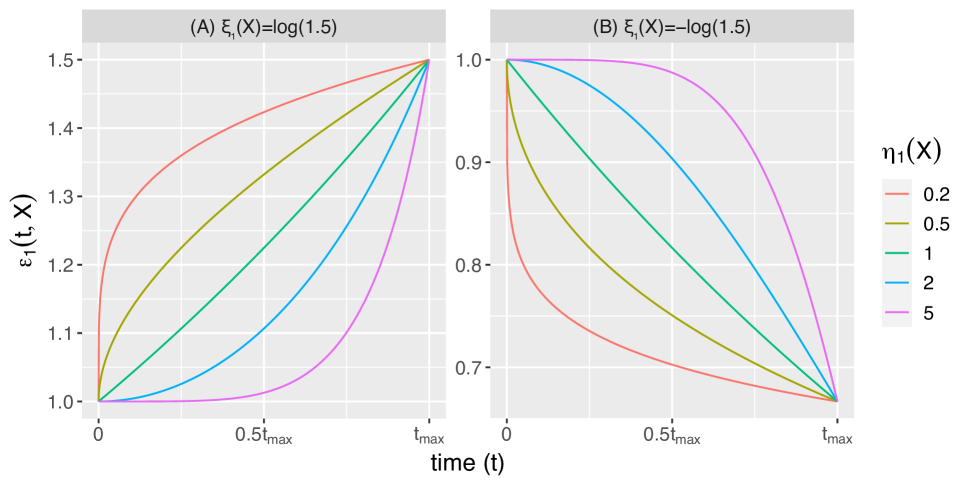
Figure 1: Graphical illustration of the sensitivity function $\varepsilon_{1}(t,\bm{X})$, when the $\xi_{1}(\bm{X})=\log(1.5)$ (Panel A) or $\xi_{1}(\bm{X})=-\log(1.5)$ (Panel B), with $\eta_{1}(\bm{X})\in\{0.2,0.5,1,2,5\}$.

When $\varepsilon_{0}(t,\bm{X})\neq 1$ or $\varepsilon_{1}(t,\bm{X})\neq 1$, the proposed single and multiply robust estimators in Section 3 will in theory be biased. However, we introduce the following weights based on the sensitivity functions to restore unbiased estimation of PSCE:

$$\widehat{w}_{1,c}(t,\bm{X})=\frac{\varepsilon_{1}(t,\bm{X})e_{c}(\bm{X};\widehat{\bm{\gamma}})+\varepsilon_{1}(t,\bm{X})e_{a}(\bm{X};\widehat{\bm{\gamma}})}{\varepsilon_{1}(t,\bm{X})e_{c}(\bm{X};\widehat{\bm{\gamma}})+e_{a}(\bm{X};\widehat{\bm{\gamma}})},\quad\widehat{w}_{1,a}(t,\bm{X})=\frac{e_{c}(\bm{X};\widehat{\bm{\gamma}})+e_{a}(\bm{X};\widehat{\bm{\gamma}})}{\varepsilon_{1}(t,\bm{X})e_{c}(\bm{X};\widehat{\bm{\gamma}})+e_{a}(\bm{X};\widehat{\bm{\gamma}})},$$

$$\widehat{w}_{0,n}(t,\bm{X})=\frac{e_{c}(\bm{X};\widehat{\bm{\gamma}})+e_{n}(\bm{X};\widehat{\bm{\gamma}})}{\varepsilon_{0}(t,\bm{X})e_{c}(\bm{X};\widehat{\bm{\gamma}})+e_{n}(\bm{X};\widehat{\bm{\gamma}})},\quad\widehat{w}_{0,c}(t,\bm{X})=\frac{\varepsilon_{0}(t,\bm{X})e_{c}(\bm{X};\widehat{\bm{\gamma}})+\varepsilon_{0}(t,\bm{X})e_{n}(\bm{X};\widehat{\bm{\gamma}})}{\varepsilon_{0}(t,\bm{X})e_{c}(\bm{X};\widehat{\bm{\gamma}})+e_{n}(\bm{X};\widehat{\bm{\gamma}})}.$$

In Web Appendix D.1, we generalize Result 1 to the scenario with $\varepsilon_{1}(t,\bm{X})$ or $\varepsilon_{1}(t,\bm{X})\neq 1$ by including the additional weights $\{\widehat{w}_{1,c}(u,\bm{X}),\widehat{w}_{0,c}(u,\bm{X})\}$ to remove the bias due to violation of Assumption 3. The explicit forms of the bias-corrected singly robust estimators are developed in Web Appendix D.1. In Web Appendix D.2, we generalize the multiply robust estimator, $\widehat{\mathcal{S}}_{z,g}^{mr}(\bm{X})$, by rewighting the original estimator with the weights $\widehat{w}_{z,g}(t,\bm{X})$; for example, the new expression of $\widehat{\mathcal{S}}_{1,c}^{mr}(\bm{X})$, i.e., the first componment in $\widehat{\Delta}_{g}^{mr}(\bm{X})$, is

$$\widehat{\mathcal{S}}_{1,c}^{mr}(u)$$

$$= \mathbb{P}_{n}\Bigg{\{}\widehat{w}_{1,c}(u,\bm{X})\frac{e_{c}(\bm{X};\widehat{\bm{\gamma}})}{\widehat{p}_{1}-\widehat{p}_{0}}\frac{S}{p_{1}(\bm{X};\widehat{\bm{\gamma}}_{1})}\frac{Z}{\pi(\bm{X};\widehat{\bm{\alpha}})}\left[\frac{\mathbb{I}(U\geq u)}{\mathcal{S}_{11}^{C}(u|\bm{X};\widehat{\bm{\theta}}_{11})}\!+\!\mathcal{S}_{11}(u|\bm{X};\widehat{\bm{\beta}}_{11})\int_{0}^{u}\!\!\frac{d\widehat{M}_{11}^{C}(r|\bm{X})}{\mathcal{S}_{11}(r|\bm{X};\widehat{\bm{\beta}}_{11})\mathcal{S}_{11}^{C}(r|\bm{X};\widehat{\bm{\theta}}_{11})}\right]$$

$$\quad+\frac{\widehat{w}_{1,c}^{2}(u,\bm{X})}{\varepsilon_{1}(u,\bm{X})}\frac{\mathcal{S}_{11}(u|\bm{X};\widehat{\bm{\beta}}_{11})}{\widehat{p}_{1}-\widehat{p}_{0}}\left[\frac{1-Z}{1-\pi(\bm{X};\widehat{\bm{\alpha}})}(S-p_{0}(\bm{X};\widehat{\bm{\gamma}}_{0}))+\frac{p_{0}(\bm{X};\widehat{\bm{\gamma}})}{p_{1}(\bm{X};\widehat{\bm{\gamma}}_{1})}\frac{Z}{\pi(\bm{X};\widehat{\bm{\alpha}})}(p_{1}(\bm{X};\widehat{\bm{\gamma}})-S)\right]$$

$$\quad+\widehat{w}_{1,c}(u,\bm{X})\frac{e_{c}(\bm{X})}{\widehat{p}_{1}-\widehat{p}_{0}}\left(1-\frac{Z}{\pi(\bm{X};\widehat{\bm{\gamma}})}\right)\mathcal{S}_{11}(u|\bm{X};\widehat{\bm{\beta}}_{11})\Bigg{\}}.$$ (10)

The following result summarizes the properties of such bias-corrected multiply robust estimators, where the technical details are provided in Web Appendix D.3.

Result 3 (Double robustness under violation of principal ignorability)

Suppose that assumptions 1–2 and 4 hold and the sensitivity functions $\{\varepsilon_{1}(t,\bm{X}),\varepsilon_{0}(t,\bm{X})\}$ are known. For all $z\in\{0,1\}$ and $g\in\{c,n,a\}$, $\widehat{\mathcal{S}}_{z,g}^{mr}(u)$ developed in Web Appendix D.2 is a doubly robust estimator for $\mathcal{S}_{z,g}(u)$ in the sense that $\widehat{\mathcal{S}}_{z,g}^{mr}(u)$ is consistent to $\mathcal{S}_{z,g}(u)$ under the union model $\mathcal{M}_{\pi+e+C}\cup\mathcal{M}_{e+T}$. As a consequence, $\widehat{\Delta}_{g}^{mr}(u)=\widehat{\mathcal{S}}_{1,g}^{mr}(u)-\widehat{\mathcal{S}}_{0,g}^{mr}(u)$ is also doubly robust and consistent to $\Delta_{g}(u)$ under $\mathcal{M}_{\pi+e+C}\cup\mathcal{M}_{e+T}$ for all $g\in\{c,n,a\}$.

Notice that $\widehat{\mathcal{S}}_{z,g}^{mr}(u)$ (and $\widehat{\Delta}_{g}^{mr}(u)$) is a doubly robust estimator in the sense that it can provide consistent estimation under either $\mathcal{M}_{\pi+e+C}$ or $\mathcal{M}_{e+T}$. In a randomized trial such as ADAPTABLE, however, we can always consistently estimate $\mathcal{M}_{\pi}$ by a working logistic regression $\pi(\bm{X};\widehat{\bm{\alpha}})$ due to randomization. In that case, $\widehat{\mathcal{S}}_{z,g}^{mr}(u)$ (and $\widehat{\Delta}_{g}^{mr}(u)$) remains doubly robust and is consistent under the union model $\mathcal{M}_{e+C}\cup\mathcal{M}_{e+T}$. To conduct the sensitivity analysis, one can report $\widehat{\mathcal{S}}_{z,g}^{mr}(u)$ or $\widehat{\Delta}_{g}^{mr}(u)$ over a range of values of $\{\xi_{1}(\bm{X}),\xi_{0}(\bm{X})\}$, which capture how the PSCE estimates are affected by deviations from Assumption 3.

4.2 Violation of monotonicity

If the monotonicity assumption (Assumption 2) does not hold, we cannot rule out defiers and we four principal strata $G=\{c,n,a,d\}$ need to be considered for estimating PSCEs. We consider the sensitivity function proposed in Ding and Lu (2017) to capture the deviation from monotonicity:

$$\zeta(\bm{X})=\frac{\mathbb{P}(G=d|\bm{X})}{\mathbb{P}(G=c|\bm{X})},$$

which takes values from 0 to $\infty$. The sensitivity function is $\zeta(\bm{X})$ is the ratio between the probabilities of defiers and compliers conditional on $\bm{X}$. When $\zeta(\bm{X})=0$, then monotonicity holds, but $\zeta(\bm{X})>0$ implies that the defier strata cannot be ignored. With a fixed value of $\zeta(\bm{X})$, we have then developed bias-corrected estimators for $\mathcal{S}_{z,g}(u)$, $z\in\{0,1\}$ and $g=\{c,n,a,d\}$ in Web Appendix E. Importantly, the multiply robust estimators, $\widehat{\mathcal{S}}_{z,g}^{mr}(u)$, given in Web Appendix E.2 remain triply robust under the union model $\mathcal{M}_{\pi+e+C}\cup\mathcal{M}_{\pi+T}\cup\mathcal{M}_{e+T}$, as summarized in the following result (proof provided in Web Appendix E.3).

Result 4 (Multiple robustness in the presence of defiers)

Suppose $\zeta(\bm{X})$ is known and Assumptions 1, 4 and the generalized principal ignorability assumption (Assumption 5 in Web Appendix E) hold. For all $z\in\{0,1\}$ and $g\in\{c,n,a,d\}$, $\widehat{\mathcal{S}}_{z,g}^{mr}(u)$ developed in Web Appendix E.2 is a triply robust estimator for $\mathcal{S}_{z,g}(u)$ in the sense that $\widehat{\mathcal{S}}_{z,g}^{mr}(u)$ is consistent to $\mathcal{S}_{z,g}(u)$ under the union model $\mathcal{M}_{\pi+e+C}\cup\mathcal{M}_{\pi+T}\cup\mathcal{M}_{e+T}$. As a consequence, $\widehat{\Delta}_{g}^{mr}(u)=\widehat{\mathcal{S}}_{1,g}^{mr}(u)-\widehat{\mathcal{S}}_{0,g}^{mr}(u)$ is also consistent to $\Delta_{g}(u)$ under $\mathcal{M}_{\pi+e+C}\cup\mathcal{M}_{\pi+T}\cup\mathcal{M}_{e+T}$ for all $g\in\{c,n,a\}$.

Similar to Section 4.1, one can report $\widehat{\mathcal{S}}_{z,g}^{mr}(u)$ or $\widehat{\Delta}_{g}^{mr}(u)$ over a range of values of $\zeta(\bm{X})$, which help assess how the PSCE estimates are affected by departures from Assumption 2.

5 Applications to the ADAPTABLE pragmatic trial

5.1 Description of data and intention-to-treat analysis

We evaluate the comparative effectiveness of two aspirin dosing strategies, 325 mg versus 81 mg per day, in the ADAPTABLE trial. The ADAPTABLE trial began patient enrollment in 2016, and included 15,076 participants with established atherosclerotic cardiovascular disease that were randomly assigned in a 1:1 ratio to take the high dose and low dose. The participants were followed up until June 2020, with a median duration of follow-up time at 26 months and an interquartile range from 19 to 35 months. During follow up, 2,493 paticipants withdrew consent from study or discontinued aspirin intake, and were excluded from our analysis. Table 1 summarizes the baseline covariates among the $n=10,030$ complete-case participants that we used for our analysis to illustrate the main issue of noncompliance. Our data include all participants who neither have missing values in their baseline characteristics nor drop out from the study. In our dataset, all baseline characteristics are well balanced, ensuring to a certain extent that the exclusion of incomplete cases does not lead to systematic difference between the compliance groups.

Table 1: Mean and standard deviation of baseline characteristics stratified by the treatment assignment. ASD is the absolute standardized difference between patients assigned to the 325-mg group and those assigned to the 81-mg group. Given a specific baseline covariate, its ASD is calculated as ${|\bar{x}_{1}-\bar{x}_{0}|}/{\sqrt{0.5(s_{1}^{2}+s_{0}^{2})}}$, where $\bar{x}_{z}$ and $s_{z}^{2}$ are the mean and variance of this covariate within the 325-mg group ($z=1$) or the 81-mg group ($z=0$).

	81-mg Group	325-mg Group	ASD
Variable	(sample size $5239$)	(sample size $4791$)
Age (years)	67.00 (9.45)	66.77 (9.32)	0.02
Female sex	0.29 (0.46)	0.31 (0.46)	0.04
White race	0.84 (0.37)	0.85 (0.36)	0.02
Hispanic ethnicity	0.03 (0.18)	0.03 (0.17)	0.01
Non-internet users	0.15 (0.35)	0.14 (0.35)	0.02
Current smokers	0.09 (0.29)	0.10 (0.30)	0.01
P2Y12 inhibitor	0.23 (0.42)	0.23 (0.42)	0.00
Medical History
Myocardial infarction	0.37 (0.48)	0.36 (0.48)	0.01
Atrial fibrillation	0.08 (0.27)	0.09 (0.28)	0.03
Percutaneous coronary intervention	0.42 (0.49)	0.42 (0.49)	0.01
Coronary artery disease	0.95 (0.21)	0.96 (0.20)	0.04
Coronary‐artery bypass grafting	0.25 (0.44)	0.25 (0.43)	0.02
Hypertension	0.87 (0.34)	0.87 (0.33)	0.01
Hyperlipidemia	0.90 (0.30)	0.91 (0.29)	0.01
Peripheral artery disease	0.24 (0.43)	0.25 (0.44)	0.03
Congestive heart failure	0.23 (0.42)	0.25 (0.43)	0.04
History of bleeding	0.08 (0.28)	0.09 (0.29)	0.03
Aspirin use prior to randomization
Prior dose: 81 mg	0.85 (0.36)	0.86 (0.35)	0.02
Prior dose: 325 mg	0.12 (0.33)	0.12 (0.33)	0.01

Similar to the primary report of ADAPTABLE, we consider the primary outcome to be the time to first occurrence of death from any reason and hospitalization from stroke or myocardial infarction. We restrict the maximum follow-up time at $t_{\max}=38$ months after randomization, and censor any outcomes beyond this point. The outcome occurred in 358 participants in the low-dose arm (event rate 7.5%) and 386 participants in the high-dose arm (event rate 7.4%). We performed an ITT analysis to estimate the differences of counterfactural survival functions based on the doubly robust approach developed in Bai et al. (2013), where Cox proportional hazard regression was used to model the arm-specific time-to-censoring and time-to-event process conditional on all pre-randomization covariates in Table 1. The ITT results are provided in Web Figure 1 (all Web Figures are available in Supplementary Material), and suggest no differences between these two aspirin dosages on the time-to-event outcome (the two counterfactual survival functions almost overlapped). The ITT analysis, however, does not take treatment noncompliance into consideration, and offer no insights into potential treatment effect heterogeneity across subpopulations defined by compliance patterns. In ADAPTABLE, 38.0% of patients who were assigned to the high-dose arm took the low-dose and 6.5% of patients who were assigned to the low-dose arm took the high-dose, and we apply the proposed methods to investigate the PSCE estimands defined for compliers, always high-dose and always low-dose takers.

5.2 Model specification, balance check and strata characteristics

The four working models described in Section 3.1 are used to estimate the treatment assignment process, noncompliance status, the time to censoring, and the time to outcome in the ADAPTABLE trial, adjusting for all baseline characteristics in Table 1. In particular, the working logistic propensity score model is fitted for adjusting any chance imbalance in baseline covariates, rather than addressing confounding due to assignment.

While the treatment is considered randomized, the noncompliance behavior is not randomized and the principal score models are fitted to address compliance-outcome confounding. To check adequacy of the principal score models, we empirically assess the balance for each baseline covariate across before and after principal score weighting; this step is analogous to balance check for propensity score weighted analysis of observational studies (Li et al., 2018). Specifically, we extend the strategy in Ding and Lu (2017) by defining the following three balancing metrics to quantify the weighted standardized mean differences (SMD) of a given covariate $X$ across the four observed $(Z,S)$ cell, $(Z=1,S=1)$, $(Z=0,S=1)$, $(Z=1,S=0)$, and $(Z=0,S=0)$:

$$\text{SMD}_{c} =\frac{1}{s_{c}}\left|\mathbb{P}_{n}\left[\frac{ZS\mathcal{W}_{1,c}(\bm{X})X}{\mathbb{P}_{n}[ZS]}-\frac{(1-Z)(1-S)\mathcal{W}_{0,c}(\bm{X})X}{\mathbb{P}_{n}[(1-Z)(1-S)]}\right]\right|,$$

$$\text{SMD}_{n} =\frac{1}{s_{n}}\left|\mathbb{P}_{n}\left[\frac{Z(1-S)\mathcal{W}_{1,n}(\bm{X})X}{\mathbb{P}_{n}[Z(1-S)]}-\frac{(1-Z)(1-S)\mathcal{W}_{0,n}(\bm{X})X}{\mathbb{P}_{n}[(1-Z)(1-S)]}\right]\right|,$$

$$\text{SMD}_{a} =\frac{1}{s_{a}}\left|\mathbb{P}_{n}\left[\frac{ZS\mathcal{W}_{1,a}(\bm{X})X}{\mathbb{P}_{n}[ZS]}-\frac{(1-Z)S\mathcal{W}_{0,a}(\bm{X})X}{\mathbb{P}_{n}[(1-Z)S]}\right]\right|,$$

where $\mathcal{W}_{z,g}(\bm{X})$ for $z\in\{0,1\}$ and $g\in\{c,a,n\}$ are weights, the normalization factor is defined as $s_{c}=\sqrt{\frac{s_{11}^{2}+s_{00}^{2}}{2}}$, $s_{n}=\sqrt{\frac{s_{10}^{2}+s_{00}^{2}}{2}}$, $s_{a}=\sqrt{\frac{s_{11}^{2}+s_{01}^{2}}{2}}$, and $s_{zs}^{2}$ is the empirical variance of $X$ within all subjects in the $(Z=z,S=s)$ cell. By definition, $\text{SMD}_{c}$ quantifies the weighted mean difference of $X$ between the $(Z=1,S=1)$ and $(Z=0,S=0)$ cells, $\text{SMD}_{n}$ quantifies the weighted mean difference of $X$ between the $(Z=1,S=0)$ and $(Z=0,S=0)$ cells, and $\text{SMD}_{a}$ quantifies the weighted mean difference of $X$ between the $(Z=1,S=1)$ and $(Z=0,S=1)$ cells. When $\mathcal{W}_{z,g}(\bm{X})\equiv 1$, the SMDs measure the systematic difference across different $(Z,S)$-strata, and therefore reflects the amount of confounding due to noncompliance. When $\mathcal{W}_{z,g}(\bm{X})$ is specified as the corresponding principal score weights, that is, $\mathcal{W}_{1,c}(\bm{X})=\frac{e_{c}(\bm{X};\widehat{\bm{\gamma}})}{p_{1}(\bm{X};\widehat{\bm{\gamma}}_{1})}\Big{/}\frac{\widehat{e}_{c}}{\widehat{p}_{1}}$, $\mathcal{W}_{0,c}(\bm{X})=\frac{e_{c}(\bm{X};\widehat{\bm{\gamma}})}{1-p_{0}(\bm{X};\widehat{\bm{\gamma}}_{0})}\Big{/}\frac{\widehat{e}_{c}}{1-\widehat{p}_{0}}$, $\mathcal{W}_{1,n}(\bm{X})=1$, $\mathcal{W}_{0,n}(\bm{X})=\frac{e_{n}(\bm{X};\widehat{\bm{\gamma}})}{1-p_{0}(\bm{X};\widehat{\bm{\gamma}}_{0})}\Big{/}\frac{\widehat{e}_{n}}{1-\widehat{p}_{0}}$, and $\mathcal{W}_{1,a}(\bm{X})=\frac{e_{a}(\bm{X};\widehat{\bm{\gamma}})}{p_{1}(\bm{X};\widehat{\bm{\gamma}}_{0})}\Big{/}\frac{\widehat{e}_{a}}{\widehat{p}_{1}}$, $\mathcal{W}_{0,a}(\bm{X})=1$, the SMDs quantifies the extent to which the confounding is addressed by weighting. In theory, if the principal score models are correctly specified, the SMDs after the weighting converges to 0, and therefore can be used as a diagnostic check for $e_{g}(\bm{X};\bm{\gamma})$.

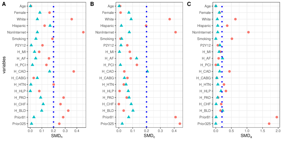
Figure 2: Balance check for baseline characteristics for $\text{SMD}_{n}$ (panel A), $\text{SMD}_{c}$ (panel B), and $\text{SMD}_{a}$ (panel C). The red ‘$\bullet$’ symbol indicates the unweighted SMDs and the blue ‘$\blacktriangle$’ symbol indicates principal score weighted SMDs. The vertical axis shows the names of the variables. Abbreviations: NonInternet - non-internet users; Smoking: current smokers; P2Y12: P2Y12 inhibitor; H_MI: Myocardial infarction; H_AF: Atrial fibrillation; H_PCI: Percutaneous coronary intervention; H_CAD: Coronary artery disease; H_CABG: coronary‐artery bypass grafting; H_HTN: Hypertension; H_HLP: Hyperlipidemia; H_PAD: peripheral artery disease; H_CHF: congestive heart failure; H_BLD: History of bleeding; Prior81: Prior aspirin dose - 81 mg; Prior325: Prior aspirin dose - 325 mg.

Figure 2 provides the love plots of the $\text{SMD}_{c}$, $\text{SMD}_{n}$, and $\text{SMD}_{a}$ for all baseline characteristics before and after principal score weighting. A vertical line is superimposed on this figure to denote a standardized difference of 20%, which we chose as a threshold for adequate balance. It is evident that the principal score weighting improves the balance of baseline characteristics across the $(Z,S)$-strata. The SMDs after principal score weighting are generally controlled below 20%, where the only exceptions are the $\text{SMD}_{c}$ of the coronary artery disease and the $\text{SMD}_{a}$ of the atrial fibrillation and history of bleeding are slightly (at 21%, 22%, and 22%, respectively). Further inspections indicate that the prevalence of these 3 covariates are either close to 0 or 1, and additional attempts on including interactions into the principal score models has limited improvements on the SMD. Therefore we consider the fitted principal score models adequate.

Table 2: Mean and standard deviation of baseline characteristics among tha always low-dose takers, compliers, and always high-dose takers. Max ASD is the maximum pairwise absolute standardized difference across the three principal strata. Given a specific baseline covariate, its Max ASD is calculated as the maximum of ${|\bar{x}_{g}-\bar{x}_{g^{\prime}}|}/{\sqrt{0.5(s_{g}^{2}+s_{g^{\prime}}^{2})}}$ for all $g,g^{\prime}\in\{c,n,a\}$, where $\bar{x}_{g}$ and $s_{g}^{2}$ are the estimated mean and variance of this covariate in the stratum $g$.

Variable	Always low-dose	Compliers	Always high-dose	Max
	takers		takers	ASD
Expected sample size	3811	5577	642
Age (years)	67.70 (9.34)	66.44 (9.36)	66.02 (9.56)	0.18
Female sex	0.32 (0.47)	0.29 (0.45)	0.28 (0.45)	0.09
White race	0.78 (0.41)	0.89 (0.31)	0.80 (0.40)	0.29
Hispanic ethnicity	0.04 (0.20)	0.03 (0.16)	0.04 (0.19)	0.08
Non-internet users	0.21 (0.41)	0.09 (0.28)	0.24 (0.42)	0.41
Current smokers	0.10 (0.31)	0.08 (0.28)	0.14 (0.35)	0.18
P2Y12 inhibitor	0.25 (0.43)	0.22 (0.41)	0.22 (0.42)	0.07
Medical History
Myocardial infarction	0.39 (0.49)	0.35 (0.48)	0.38 (0.49)	0.09
Atrial fibrillation	0.09 (0.28)	0.08 (0.27)	0.10 (0.30)	0.09
Percutaneous coronary intervention	0.46 (0.50)	0.40 (0.49)	0.39 (0.49)	0.15
Coronary artery disease	0.96 (0.19)	0.95 (0.21)	0.94 (0.24)	0.12
Coronary‐artery bypass grafting	0.26 (0.44)	0.25 (0.43)	0.25 (0.43)	0.02
Hypertension	0.89 (0.32)	0.85 (0.35)	0.90 (0.30)	0.13
Hyperlipidemia	0.91 (0.28)	0.90 (0.30)	0.88 (0.32)	0.10
Peripheral artery disease	0.29 (0.45)	0.22 (0.41)	0.25 (0.44)	0.16
Congestive heart failure	0.27 (0.44)	0.22 (0.41)	0.26 (0.44)	0.12
History of bleeding	0.11 (0.31)	0.07 (0.26)	0.10 (0.30)	0.12
Aspirin use prior to randomization
Prior dose: 81 mg	0.90 (0.30)	0.87 (0.34)	0.45 (0.50)	1.11
Prior dose: 325 mg	0.08 (0.27)	0.11 (0.32)	0.47 (0.50)	0.97

Based on the principal score estimates, we calculate the proportion of the three principal strata. The always low-dose takers and compliers constitute the majority of study population (38.0% and 55.6%), and 6.4% of the study population are always high-dose takers. To provide further intuitions on each subpopulation, Table 2 summarizes the moments of baseline characteristic for each principal stratum. The estimated mean of a baseline covariate $X\in\bm{X}$ in a specific stratum $g\in\{a,c,n\}$ is calculated by $\bar{x}_{g}=\mathbb{P}_{n}[\frac{e_{g}(\bm{X};\widehat{\bm{\gamma}})}{\widehat{e}_{g}}X]$. Similarly, the estimated standard deviation of $X$ in the stratum $g$ is obtained by the square root of $\mathbb{P}_{n}[\frac{e_{g}(\bm{X};\widehat{\bm{\gamma}})}{\widehat{e}_{g}}(X-\bar{x}_{g})^{2}]$. The baseline characteristics appear to be substantially different across principal strata, as quantified by the maximum pairwise absolute standardized difference (Li and Li, 2019) in the last column of Table 2. For example, the always low-dose takers are older and include slightly more female patients than the compliers and the always high-dose takers. The compliers include fewer non-internet users and more white patients. The always high-dose takers are the youngest but more smokers. In addition, the always low-dose takers appear to be more likely to have cardiovascular disease histories, with higher prevalence of peripheral artery disease, percutaneous coronary intervention, and bleeding history (less healthier subpopulation). Moreover, aspirin use prior to randomization is strongly associated with the aspirin use during the trial and is a strong predictor for the principal strata membership.

5.3 Assessing principal survival causal effects

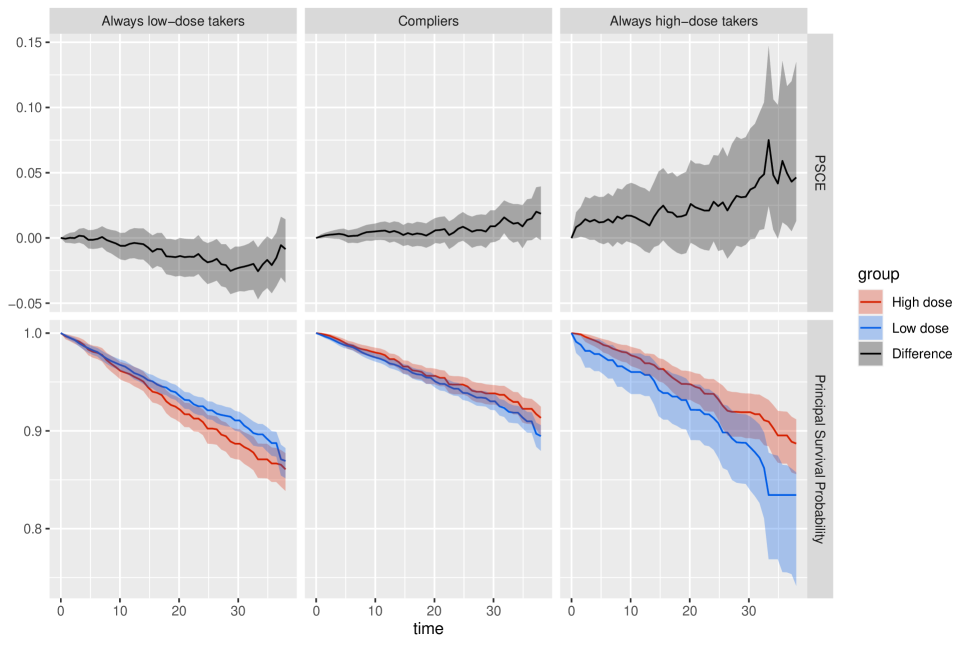
Figure 3: The principal survival causal effects (PSCEs) and the corresponding counterfactual survival functions among the always low-dose takers, compliers, and always high-dose takers, evaluated over 50 equally-spaced grid values. The 95% confidence bands are based on 1000 bootstrap replicates.

Figure 3 presents the PSCE estimates using the proposed multiply robust estimators, along with the counterfactual survival functions within each principal stratum. The point-wise 95% confidence bands are obtained by the nonparametric bootstrap with $B=1,000$ replicates. The results suggest the heterogeneity of causal effects across strata which contributes to the null ITT effect. In particular, the counterfactual survival functions are more separated (compared to ITT) once we stratify by noncompliance patterns. For the always low-dose takers, assignment to the high-dose group leads to a lower survival probability; the magnitude of PSCE peaks at around 33 months ($\widehat{\Delta}_{n}^{mr}(33)=-0.025$ with 95% CI from -0.047 to -0.007). For the compliers, however, assignment to the high-dose group has a protective effect on survival during the entire follow-up time. The magnitude of PSCE increases over time but the 95% confidence band generally includes 0. For the always high-dose takers, assignment to the high-dose arm provides the strongest protective effect on patients’ risk on death and hospitalization, and the magnitude of PSCE increases over time. For example, the PSCE among the always high-dose takers increases from 0.016 (95% CI: -0.011,0.047) at 18 months follow-up to 0.059 (95% CI: 0.012,0.145) at 36 months follow-up. However, the confidence interval for the always high-dose stratum is wider than the other two strata, possibly due to its small sample size (6.4% of total population are always high-dose takers). In summary, we identify a protective effect due to the high dose strategy among the compliers, and provide preliminary evidence for efficacy. In addition, there appears to be an opposite effect due to assignment to the high-dose arm among the always low-dose takers and the always high-dose takers, possibly due to unmeasured factors and medications for patients in those strata. The nonzero direct effects among these two strata indicate that the commonly-use ER assumption may not be plausible in the ADAPTABLE trial.

5.4 Sensitivity analysis for principal ignorability

To better interpret the analysis in Section 5.3, we first examine the sensitivity of PSCE estimates under violations of the principal ignorability assumption. Resuming notation from Section 4.1, we consider constant values $\{\xi_{1},\xi_{0}\}$ for the extremum parameters and fix the two curvature parameters to 1 (i.e., $\eta_{1}(\bm{X})=\eta_{0}(\bm{X})=1$); this assumes that the sensitivity functions $\varepsilon_{1}(t,\bm{X})$ and $\varepsilon_{0}(t,\bm{X})$ changes at a constant rate during the follow-up time. Due to low event rate (7.4% at $t_{\max}=38$ months), if the counterfactual survival function in one stratum is 10% larger or 10% lower than its counterpart in another stratum at the maximum of follow-up time, one of the counterfactual survival function may exceed 1 and hence becomes invalid. Therefore, we only allow $(\xi_{1},\xi_{0})$ to vary within the region $[\log(0.9),\log(1.1)]\times[\log(0.9),\log(1.1)]$ as an exploratory sensitivity analysis.

Table 2 suggests that the always low-dose takers are older and are generally the least healthiest, followed by the the compliers and then the always high-dose takers. If this pattern persists and can be further attributed to unmeasured factors that affect survival, the extremum parameters should be restricted such that $\xi_{1}<0$ and $\xi_{0}>0$. Intuitively, this would be the case if unhealthier patients at baseline concern about adverse effects that may occur due to taking the high dose, and therefore healthier patients are more willing to be adhere to the high-dose assignment. Under this avoid-harm scenario, Figure 4 presents the PSCE estimates at four values of $(\xi_{1},\xi_{0})$ within the region $[\log(0.9),0)\times(0,\log(1.1)]$. We observe that $\widehat{\Delta}_{a}^{mr}(u)$ is more robust to such violation of principal ignorability, as $\widehat{\Delta}_{a}^{mr}(u)$ is always positive (95% confidence bands exclude zero) for different values of $(\xi_{1},\xi_{0})$. In contrast, $\widehat{\Delta}_{c}^{mr}(u)$ and $\widehat{\Delta}_{n}^{mr}(u)$ are more sensitive to different values of $(\xi_{1},\xi_{0})$ and there exists a tipping point. Specifically, the point estimates, $\widehat{\Delta}_{n}^{mr}(u)$ and $\widehat{\Delta}_{c}^{mr}(u)$ for $u\leq t_{\max}$ generally attenuate toward the null when $\xi_{0}=\log(1.05)$ and can move to the opposite direction when $\xi_{0}=\log(1.1)$. In other words, an unmeasured factor that contributes to 5% higher (on a relative scale) survival among compliers relative to the always low-dose takers (adjusting for all other observed covariates) can explain away the observed causal effects among the compliers and the always low-dose takers strata.

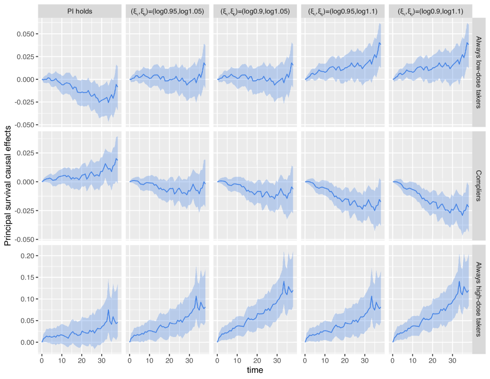
Figure 4: Sensitivity of the PSCEs to the violation of the principal ignorability assumption, under the hypothetical scenario that the always low-dose takers are the unhealthiest group and the always high-dose takers are the healthiest group. The PSCEs under principal ignorability assumption are included in the first column for ease of comparison.

We further consider an opposite scenario by restricting the extremum parameters within $\xi_{1}>0$ and $\xi_{0}<0$ such that the always low-dose takers are the healthiest and the always high-dose takers are the unhealthiest due to unmeasured factors. Intuitively, this scenario would occur if patients with more comorbidity consider the high-dose medication as the last resort and there are no better alternative medications. Under this last-resort scenario, the estimated PSCEs at four values of $(\xi_{1},\xi_{0})$ within the region $(0,\log(1.1)]\times[\log(0.9),0)$ are summarized in Web Figure 2. We observe that $\widehat{\Delta}_{c}^{mr}(u)$ and $\widehat{\Delta}_{n}^{mr}(u)$ are generally robust to this specific type of violation of principal ignorability. The effect estimates $\widehat{\Delta}_{c}^{mr}(u)$ and $\widehat{\Delta}_{n}^{mr}(u)$ become even stronger as we vary the sensitivity parameters and their 95% confidence bands often exclude zero. However, $\widehat{\Delta}_{a}^{mr}(u)$ attenuates toward the null when $\xi_{1}$ and $\xi_{0}$ deviates from 0, and the associated 95% confidence bands straddle the null.

5.5 Sensitivity analysis for monotonicity

While there is little empirical grounds to indicate the existence of defiers, the monotonicity assumption is unverifiable from the observed data alone. We therefore further consider a sensitivity function defined in Section 4.2. For simplicity, we assume $\zeta(\bm{X})=\zeta$ does not depend on baseline covariates, and choose values of $\zeta$ under the range suggested in Proposition 2 of the Supplementary Material to ensure that the proportion of each principal stratum is not negative. Specifically, our previous analysis suggests that $\widehat{p}_{1}=0.620$ and $\widehat{p}_{0}=0.064$, and therefore the range of $\zeta$ are expected to lie between $\left[0,1-\frac{\widehat{p}_{1}-\widehat{p}_{0}}{\min(\widehat{p}_{1},1-\widehat{p}_{0})}\right]=[0,0.103]$. This range motivates us to explore $\zeta=\{0,0.05,0.08,0.09\}$, and we present the results of $\widehat{\Delta}_{g}^{mr}(u)$ under each $\zeta$ in Web Figure 3. The results imply that the PSCE estimates among the always low-dose takers and compliers are robust even if there exist defiers. The PSCE among the always high-dose takers, however, are relatively sensitive of $\zeta$. As $\zeta$ increases, $\widehat{\Delta}_{a}^{mr}(u)$ is further attenuated toward the null and the 95% confidence bands also increase with a larger $\zeta$. This is likely because the existence of defiers reduce the sample size for the always high-dose takers, increasing the uncertainty for the PSCE among the always high-dose takers.

6 Discussion

We provide a general approach for identification of the principal causal effects in the presence of treatment noncompliance with a right-censored time-to-event outcome. Our approach is particularly useful when the exclusion restriction assumption is likely not plausible. Instead of using the exclusion restriction, we leverage the principal ignorability assumption and develop a multiply robust approach to identify the PSCE. The multiply robust estimator offers additional protection on model misspecification and represents a principled approach to integrate different identification formulas for the PSCE. We implement the multiply robust estimator to the ADAPTABLE study, and our analysis of the ADAPTABLE trial reveals that the heterogeneity of the average causal effects across principal strata likely contributes to the null effect under the ITT analysis. In particular, we observe a small efficacy signal due to the high-dose aspirin medication among compliers who would always take the assigned treatment. However, the direct effect of assignment has an opposite direction among the always high-dose takers and always low-dose takers, possibly due to unmeasured factors. These results suggest the need to further investigate the mechanisms for such treatment effect heterogeneity across the study subpopulations.

We recognize that the analysis of ADAPTABLE trial relies on two key identification assumptions required for studying noncompliance. First, the principal ignorability assumption is only appropriate when sufficient baseline covariates have been collected to fully deconfound the relationship between noncompliance and the survival outcome of interest. Based on the assumed sensitivity parameters, we investigate to what extent the estimated PSCE may change under two types of violation of the principal ignorability assumption—the avoid-harm and the last-resort scenarios. We found that the causal effects in certain strata can be more sensitive to one type of violation than the other. For example, the avoid-harm scenario may arise when digestive disease is an unmeasured factor such that patients with digestive diseases may prefer not to take high aspirin dosage due to its risk on bleeding but having digestive disease can increase the risk of death. If the impact of such an unmeasured factor on survival leads to 5% more (on a relative scale) survival among the compliers relative to the always low-dose takers, then the observed PSCE within those two strata may be fully explained away. However, in the last-resort scenario, the PSCE within these two strata is robust to unmeasured factors and can even further deviate from the null. Second, we have also assessed the PSCE assuming the existence of defiers and the PSCE within the compliers and always low-dose takers strata are generally robust to violation of the monotonicity assumption, but the PSCE among the always high-dose takers are relatively sensitive to violation of the monotonicity, possibly due to its attenuated sample size in the presence of defiers.

By focusing on the noncompliance as a major factor that contributes to the null ITT effect, our analysis is currently restricted to a subset of the original participants in ADAPTABLE without missing baseline covariates or aspirin discontinuation. Addressing missing baseline covariates and treatment discontinuation necessitates additional structural assumptions and working models to point identify the PSCE, and it remains to be explored whether the multiply robustness property of the proposed estimator can hold in the presence of these additional complexities. While we recognize that randomization may not hold within the subset of participants without missing baseline covariates or aspirin discontinuation (say, for example, when treatment discontinuation is differential across arms), Table 1 suggests that the two arms are balanced in terms of all observed baseline covariates and does not provide clear evidence against randomization within this subset we analyzed. In addition, our development of the multiply robust estimator relies on the standard unconfoundedness assumption in observational studies, and by estimating a treatment propensity score given baseline covariates, our results should still be interpretable if conditional randomization (Assumption 1) holds.

Finally, the unbiased estimation of PSCE requires the correct specification of a certain subset of working models. We consider using finite-dimensional parametric models to estimate these nuisance models, as is commonly done in clinical research practice. When the vector of baseline covariates is high-dimensional, improved estimation of the PSCE may be possible with recent advances in the causal machine learning literature. For example, in the context of the non-censored outcomes, the multiply robust estimating function already provides a natural vehicle to integrate machine learning nuisance models, and admits an optimal estimator that achieve root-${n}$ convergence rate under cross fitting (Chernozhukov et al., 2018). Given the recent advances on causal machine learning estimators for survival data in the absence of noncompliance (Westling et al., 2023; Vansteelandt et al., 2022), expanding the current approach to integrate state-of-the-art machine learners represents a fruitful direction for future research.

Supplementary Material

The supplementary material, including the web appendices, tables, and figures, is available at https://sites.google.com/view/chaocheng.

References

- Angrist et al. (1996) Angrist, J., Imbens, G., and Rubin, D. (1996), “Identification of causal effects using instrumental variables,” Journal of the American Statistical Association, 91, 444–455.
- Bai et al. (2013) Bai, X., Tsiatis, A. A., and O’Brien, S. M. (2013), “Doubly-Robust estimators of treatment-specific survival distributions in observational studies with stratified sampling,” Biometrics, 69, 830–839.
- Baker (1998) Baker, S. G. (1998), “Analysis of survival data from a randomized trial with all-or-none compliance: estimating the cost-effectiveness of a cancer screening program,” Journal of the American Statistical Association, 93, 929–934.
- Baker and Lindeman (1994) Baker, S. G. and Lindeman, K. S. (1994), “The paired availability design: a proposal for evaluating epidural analgesia during labor,” Statistics in Medicine, 13, 2269–2278.
- Breslow (1972) Breslow, N. E. (1972), “Discussion of Professor Cox’s paper,” Journal of Royal Statistical Society: Series B (Statistical Methodology), 34, 216–217.
- Chernozhukov et al. (2018) Chernozhukov, V., Chetverikov, D., Demirer, M., Duflo, E., Hansen, C., Newey, W., and Robins, J. (2018), “Double/debiased machine learning for treatment and structural parameters,” The Econometrics Journal, 21.
- Cuzick et al. (2007) Cuzick, J., Sasieni, P., Myles, J., and Tyrer, J. (2007), “Estimating the effect of treatment in a proportional hazards model in the presence of non-compliance and contamination,” Journal of the Royal Statistical Society: Series B (Statistical Methodology), 69, 565–588.
- Ding and Lu (2017) Ding, P. and Lu, J. (2017), “Principal stratification analysis using principal scores,” Journal of the Royal Statistical Society: Series B (Statistical Methodology), 79, 757–777.
- Frangakis and Rubin (2002) Frangakis, C. and Rubin, D. (2002), “Principal Stratification in Causal Inference,” Biometrics, 58, 21–29.
- Frangakis and Rubin (1999) Frangakis, C. E. and Rubin, D. B. (1999), “Addressing complications of intention-to-treat analysis in the combined presence of all-or-none treatment-noncompliance and subsequent missing outcomes,” Biometrika, 86, 365–379.
- Gill et al. (1997) Gill, R. D., Laan, M. J., and Robins, J. M. (1997), “Coarsening at random: Characterizations, conjectures, counter-examples,” in Proceedings of the First Seattle Symposium in Biostatistics, Springer, 255–294.
- Hirano et al. (2000) Hirano, K., Imbens, G., Rubin, D., and Zhou, X.-H. (2000), “Assessing the effect of an influenza vaccine in an encouragement design,” Biostatistics, 1, 69–88.
- Imbens and Angrist (1994) Imbens, G. and Angrist, J. (1994), “Identification and estimation of local average treatment effects,” Econometrica, 62, 467–475.
- Jiang et al. (2022) Jiang, Z., Yang, S., and Ding, P. (2022), “Multiply robust estimation of causal effects under principal ignorability,” Journal of the Royal Statistical Society: Series B (Statistical Methodology), 84, 1423–1445.
- Jo and Stuart (2009) Jo, B. and Stuart, E. A. (2009), “On the use of propensity scores in principal causal effect estimation,” Statistics in Medicine, 28, 2857–2875.
- Jones et al. (2021) Jones, W. S., Mulder, H., Wruck, L. M., Pencina, M. J., Kripalani, S., Muñoz, D., Crenshaw, D. L., Effron, M. B., Re, R. N., Gupta, K., et al. (2021), “Comparative Effectiveness of Aspirin Dosing in Cardiovascular Disease,” New England Journal of Medicine, 384, 1981–1990.
- Li and Li (2019) Li, F. and Li, F. (2019), “Propensity score weighting for causal inference with multiple treatments,” The Annals of Applied Statistics, 13, 2389–2415.
- Li et al. (2018) Li, F., Morgan, K. L., and Zaslavsky, A. M. (2018), “Balancing covariates via propensity score weighting,” Journal of the American Statistical Association, 113, 390–400.
- Loeys and Goetghebeur (2003) Loeys, T. and Goetghebeur, E. (2003), “A causal proportional hazards estimator for the effect of treatment actually received in a randomized trial with all-or-nothing compliance,” Biometrics, 59, 100–105.
- Nie et al. (2011) Nie, H., Cheng, J., and Small, D. S. (2011), “Inference for the effect of treatment on survival probability in randomized trials with noncompliance and administrative censoring,” Biometrics, 67, 1397–1405.
- Robins and Finkelstein (2000) Robins, J. M. and Finkelstein, D. M. (2000), “Correcting for noncompliance and dependent censoring in an AIDS clinical trial with inverse probability of censoring weighted (IPCW) log-rank tests,” Biometrics, 56, 779–788.
- Rubin (1974) Rubin, D. B. (1974), “Estimating causal effects of treatments in randomized and nonrandomized studies.” Journal of Educational Psychology, 66, 688.
- Tsiatis (2006) Tsiatis, A. A. (2006), Semiparametric theory and missing data, Springer.
- Vansteelandt et al. (2022) Vansteelandt, S., Dukes, O., Van Lancker, K., and Martinussen, T. (2022), “Assumption-lean Cox regression,” Journal of the American Statistical Association, 1–10.
- Wei et al. (2021) Wei, B., Peng, L., Zhang, M.-J., and Fine, J. P. (2021), “Estimation of causal quantile effects with a binary instrumental variable and censored data,” Journal of the Royal Statistical Society: Series B (Statistical Methodology), 83, 559–578.
- Westling et al. (2023) Westling, T., Luedtke, A., Gilbert, P. B., and Carone, M. (2023), “Inference for treatment-specific survival curves using machine learning,” Journal of the American Statistical Association, 1–26.
- Yu et al. (2015) Yu, W., Chen, K., Sobel, M. E., and Ying, Z. (2015), “Semiparametric transformation models for causal inference in time to event studies with all-or-nothing compliance,” Journal of the Royal Statistical Society: Series B (Statistical Methodology), 77, 397.
- Zeng et al. (2021) Zeng, S., Li, F., Wang, R., and Li, F. (2021), “Propensity score weighting for covariate adjustment in randomized clinical trials,” Statistics in Medicine, 40, 842–858.