Phenomenological aspects of the fermion and scalar sectors of a $S_{4}$ flavored 3-3-1 model

Abstract

We propose a viable and predictive model based on the $SU(3)_{C}\times SU(3)_{L}\times U(1)_{X}$ gauge symmetry, supplemented by the global $U(1)_{Lg}$ symmetry, the $S_{4}$ family symmetry and several auxiliary cyclic symmetries, which successfully reproduces the observed SM fermion mass and mixing pattern. The SM charged fermion mass and quark mixing hierarchy is caused by the spontaneous breaking of the discrete symmetries, whereas the tiny active neutrino masses are generated through an inverse seesaw mechanism mediated by right-handed Majorana neutrinos. The model is consistent with the SM fermion masses and mixings and successfully accommodates the current Higgs diphoton decay rate constraints as well as the constraints arising from oblique $S$, $T$ and $U$ parameters and meson oscillations.

I Introduction

The Standard Model of particles is a widely accepted theory describing subatomic particles’ fundamental interactions. This theory has successfully explained and predicted numerous phenomena observed in particle physics experiments. Despite the great success of the Standard Model (SM), it has several unresolved problems. For example, the SM cannot explain the fermion sector’s hierarchy of masses and mixings. The range of fermion mass values extends approximately 13 orders of magnitude from the light-active neutrino mass scale up to the mass of the top quark. Whereas in the lepton sector two of the mixing angles are large and one is small, the mixing angles of the quark sector are very small, thus implying that the quark mixing matrix approaches the identity matrix. These different mass and mixing patters in the quark and lepton sectors corresponds to the SM flavor puzzle, which is not explained by the SM. In addition to this, there are other issues not explained by the SM, such as, for example, the number of families of SM fermions as well the quantization of the electric charge. Explaining the aforementioned issues motivates to consider extensions of the SM, with enlarged particle spectrum and symmetries. Possible SM extension options include models based on the $SU(3)_{C}\times SU(3)_{L}\times U(1)_{X}$ gauge group (also known as 3-3-1 models). These models have been extensively worked on in the literature Valle:1983dk ; Pisano:1991ee ; Frampton:1992wt ; Foot:1994ym ; Hoang:1995vq ; CarcamoHernandez:2005ka ; Chang:2006aa ; Hernandez:2013mcf ; CarcamoHernandez:2013krw ; Boucenna:2014ela ; CarcamoHernandez:2014wdl ; Okada:2015bxa ; Hernandez:2016eod ; Fonseca:2016tbn ; CarcamoHernandez:2017cwi ; CarcamoHernandez:2018iel ; CarcamoHernandez:2019vih ; CarcamoHernandez:2019iwh ; CarcamoHernandez:2019lhv ; CarcamoHernandez:2020ehn ; Binh:2020aal ; CarcamoHernandez:2021tlv ; Hernandez:2021zje ; Thu:2023xai because they provide an explanation of the number of fermion generations and why there are non-universal gauge assignments under the group $U(1)_{X}$ for left-handed quark fields (LH), which implies the cancellation of chiral anomalies when the number of the fermionic triplet and the anti-triplet of $SU(3)_{L}$ are equal, which occurs when the number of fermion families is a multiple of 3. Another feature of these 3-3-1 models is that the Peccei-Quinn (PQ) symmetry (a solution to the strong CP problem) is obtained, which occurs naturally, and besides that, these theories contain several sources of CP violation, and explain the quantization of the electric charge. There are two most widely used versions of 3-3-1 models, a minimal one where the lepton components are in the same triplet representation $(\nu,l,l^{C})_{L}$ and a variant where right-handed (RH) neutrinos are included in the same triplet $(\nu,l,\nu^{C})_{L}$. In addition, within the framework of 3-3-1 models, research focuses on implementing radiative Seesaw mechanisms and non-renormalizable terms through a Froggen-Nilsen (FN) mechanism to explain the pattern of mass and mixing of SM fermions. It should be noted that the FN mechanism will not produce a new break scale since the flavor break scale is the same as the symmetry break scale of the 3-3-1 model.

In this work, we propose an extension of the SM through a 3-3-1 model with (RH) neutrinos, also adding a global lepton symmetry $U(1)_{Lg}$ to ensure the conservation of the lepton number, a discrete non-abelian symmetry $S_{4}$ to reproduce the masses and mixing of the fermionic sector and three other auxiliary cyclic symmetries $Z_{4}\times Z_{4}^{\prime}\times Z_{2}$, where the $Z_{4}$ symmetry is introduced to obtain a texture with zeros in the entries of the up type quark mass matrix, in addition, the symmetry $Z_{4}^{\prime}$ together with the VEV pattern of the scalar triplets associated with the sector of charged leptons is necessary to get a diagonal charged lepton mass matrix. Finally, the $Z_{2}$ symmetry is necessary to obtain all the complete entries of the third column of the mass matrix of the down quarks and thus with the values of the VEVs of the scalars that participate in the Yukawa terms of this sector. Given that the charged lepton mass matrix is predicted to be diagonal, the lepton mixing entirely arises from the neutrino sector, where we will use an inverse seesaw mechanism Mohapatra:1986bd mediated by right-handed heavy neutrinos to generate the tiny active neutrinos masses. The $S_{4}$ symmetry group is a compelling choice due to its unique properties and its ability to efficiently describe the observed pattern of fermion masses and mixing angles in the standard model. As the smallest non-abelian group with irreducible representations of doublet, triplet, and singlet, $S_{4}$ allows for an elegant accommodation of the three fermion families. Furthermore, its cyclic structure and spontaneous breaking provide a suitable framework for generating fermion masses through mechanisms such as the Froggatt-Nielsen mechanism Froggatt:1978nt for charged fermions and the inverse seesaw mechanism Mohapatra:1986bd for light active neutrinos. The application of S 4 has demonstrated success in describing the observed patterns of SM fermion masses and mixings Altarelli:2009gn ; Bazzocchi:2009da ; Bazzocchi:2009pv ; deAdelhartToorop:2010vtu ; Patel:2010hr ; Morisi:2011pm ; Altarelli:2012bn ; Mohapatra:2012tb ; BhupalDev:2012nm ; deMedeirosVarzielas:2012apl ; Ding:2013hpa ; Ishimori:2010fs ; Ding:2013eca ; Hagedorn:2011un ; Campos:2014zaa ; Dong:2010zu ; Vien:2015fhk ; deAnda:2017yeb ; deAnda:2018oik ; CarcamoHernandez:2019eme ; CarcamoHernandez:2019iwh ; deMedeirosVarzielas:2019cyj ; DeMedeirosVarzielas:2019xcs ; Chen:2019oey ; Garcia-Aguilar:2022gfw ; CarcamoHernandez:2022vjk .

The non-abelian symmetry $S_{4}$ provides a solid theoretical framework for constructing scalar fields and understanding various phenomenologies. Scalar fields, transforming according to the representations of $S_{4}$, allow us to determine the phenomenon of meson oscillations. These oscillations are of great interest as they provide valuable information about flavor symmetry violations in the Standard Model. In addition, the scalar mass spectrum is analyzed and discussed in detail. Its analysis allows to study the implications of our model in the decay of the Standard Model like Higgs boson into a photon pair as well as in meson oscillations. Finally, besides providing new physics contribution to meson mixingz and Higgs decay into two photons, the considered model succesfully satisfies the constraints imposed by the oblique parameters, where the corresponding analysis is performed consideing the low energy effective field theory below the scale of spontaneous breaking of the $SU(3)_{L}\times U(1)_{X}\times U(1)_{L_{g}}$ symmetry. These parameters, derived from precision measurements in electroweak physics, are essential for evaluating the consistency between the theoretical model and experimental data. The consistency of our model with the oblique parameters demonstrates its ability to reproduce experimental observations in the context of electroweak physics for energy scales below $1$ TeV.

This paper is organized as follows. The section II presents the model and its details, such as symmetries, particle content, field assignments under the symmetry group, and describe the spontaneous symmetry breaking pattern. In the sections III and IV, the implications of the model in the masses and mixings in quark and lepton sectors, respectively, are discussed and analyzed. In addition, section V describes the scalar potential, the resulting scalar mass spectrum and the mixing in the scalar sector. The section VI provides an analysis and discussion of the phenomenological implications of the model in meson mixings. On the other hand, the decay rate of the Higgs to two photons is also studied in section VII. In section VIII, the contribution of the model to the oblique parameters through the masses of the new scalar fields is discussed. We state our conclusions in section IX.

II The model

The model is based on the $SU(3)_{C}\times SU(3)_{L}\times U(1)_{X}$ gauge symmetry, supplemented by the $S_{4}$ family symmetry and the $Z_{4}\times Z^{\prime}_{4}\times Z_{2}$ auxiliary cyclic symmetries, whose spontaneous breaking generates the observed SM fermion mass and mixing pattern. We also introduce a global $U(1)_{L_{g}}$ of the generalized leptonic number $L_{g}$ Chang:2006aa ; CarcamoHernandez:2017cwi ; CarcamoHernandez:2019lhv . That global $U(1)_{L_{g}}$ lepton number symmetry will be spontaneously broken down to a residual discrete lepton number symmetry $Z_{2}^{(L_{g})}$ by a VEV of the gauge-singlet scalars $\varphi$ and $\xi$ to be introduced below. The correspoding massless Goldstone bosons, the Majoron, are phenomenologically harmless since they are gauge singlets. It is worth mentioning that under the discrete lepton number symmetry $Z_{2}^{(L_{g})}$, the leptons are charged and the other particles are neutral, thus implying that in any interaction leptons can appear only in pair, thus, forbidding proton decay. The $S_{4}$ symmetry is the smallest non-Abelian discrete symmetry group having five irreducible representations (irreps), explicitly, two singlets (trivial and no-trivial), one doublet and two triplets (3 and 3’) Ishimori:2010au . While the auxiliary cyclic symmetries $Z_{4}$, $Z^{\prime}_{4}$ and $Z_{2}$ select the allowed entries of the SM fermion mass matrices that yield a viable pattern of SM fermion masses and mixings, and at the same time, the cyclic symmetries also allow a successful implementation of the inverse seesaw mechanism. The $\mathcal{G}$ chosen symmetry exhibits the following three-step spontaneous breaking:

$$\mathcal{G}=SU(3)_{C}\times SU(3)_{L}\times U(1)_{X}\times U(1)_{L_{g}}\times S_{4}\times Z_{4}\times Z_{4}^{\prime}\times Z_{2}$$ (1)

$$\Downarrow\Lambda_{\text{int }}$$

$$SU(3)_{C}\times SU(3)_{L}\times U(1)_{X}\times U(1)_{L_{g}}$$

$$\Downarrow v_{\chi}$$

$$SU(3)_{C}\times SU(2)_{L}\times U(1)_{Y}\times Z_{2}^{(L_{g})}$$

$$\ \ \ \ \ \Downarrow v_{\eta_{2}},v_{\rho}$$

$$SU(3)_{C}\times U(1)_{Q}\times Z_{2}^{(L_{g})}$$

where the different symmetry breaking scales satisfy the following hierarchy:

$$v=246\text{GeV}=\sqrt{v_{\rho}^{2}+v_{\eta_{2}}^{2}}\ll v_{\chi}\sim\mathcal{O}\left(9.9\right)\ \text{TeV}\ll\Lambda_{\textbf{int}},$$ (2)

which corresponds in our model to the VEVs of the scalar fields.
The electric charge operator is defined Valle:1983dk ; Dong:2010zu in terms of the $SU(3)$ generators $T_{3}$ and $T_{8}$ and the identity $I_{3\times 3}$ as follows:

$$Q=T_{3}+\beta T_{8}+I_{3\times 3}X.$$ (3)

where for our model we choose $\beta=-1/\sqrt{3}$, and $X$ are the charge associated with gauge group $U(1)_{X}$.

The fermionic content in this model under $SU(3)_{C}\times SU(3)_{L}\times U(1)_{X}$ Valle:1983dk ; Long:1995ctv ; CarcamoHernandez:2017cwi . The leptons are in triplets of flavor, in which the third component is an RH neutrino. The three generations of leptons for anomaly cancellation are:

$$L_{iL}=\begin{pmatrix}\nu_{i}\\ l_{i}\\ \nu_{i}^{c}\\ \end{pmatrix}_{L}\sim\left(\textbf{1},\textbf{3},-1/3\right),\quad l_{iR}\sim\left(\textbf{1},\textbf{1},-1\right),\quad N_{iR}\sim\left(\textbf{1},\textbf{1},0\right),$$ (4)

where $i=1,2,3$ is the family index. Here $\nu^{c}\equiv\nu_{R}^{c}$ is the RH neutrino and $\nu_{iL}$ are the family of neutral leptons, while $l_{iL}\ (e_{L},\mu_{L},\tau_{L})$ is the family of charged leptons, and $N_{iR}$ are three right handed Majorana neutrinos, singlets under the $3$-$3$-$1$ group. Regarding the quark content, the first two generations are antitriplet of flavor, while the third family is a triplet of flavor; note that the third generation has different gauge content compared with the first two generations, which is required by the anomaly cancellation.

$$Q_{nL}=\begin{pmatrix}d_{n}\\ -u_{n}\\ J_{n}\\ \end{pmatrix}_{L}\sim\left(\textbf{3},\overline{\textbf{3}},0\right),\quad Q_{3L}=\begin{pmatrix}u_{3}\\ d_{3}\\ T\\ \end{pmatrix}_{L}\sim\left(\textbf{3},\textbf{3},1/3\right),\quad n=1,2.$$ (5)

$$u_{iR}\sim\left(\textbf{3},\textbf{1},2/3\right),\quad d_{iR}\sim\left(\textbf{3},\textbf{1},-1/3\right),\quad J_{nR}\sim\left(\textbf{3},\textbf{1},-1/3\right),\quad T_{R}\sim\left(\textbf{3},\textbf{1},2/3\right).$$

We can observe that the $d_{iR}$ and $J_{iR}$ quarks have the same $X$ quantum number, and so are the $u_{iR}$ and $T_{R}$ quarks. Here $u_{iL}$ and $d_{iL}$ are the LH up and down type quarks fields in the flavor basis, respectively. Furthermore, $u_{iR}$ and $d_{iR}$ are the RH SM quarks, and $J_{nR}$ and $T_{R}$ are the RH exotic quarks. And the scalar sector contains four scalar triplets of flavor,

$$\rho = \begin{pmatrix}\rho_{1}^{+}\\ \frac{1}{\sqrt{2}}(v_{\rho}+\xi_{\rho}\pm i\zeta_{\rho})\\ \rho_{3}^{+}\end{pmatrix}\sim\left(\textbf{1},\textbf{3},\frac{2}{3}\right),\quad\chi\ =\ \begin{pmatrix}\chi_{1}^{0}\\ \chi_{2}^{-}\\ \frac{1}{\sqrt{2}}(v_{\chi}+\xi_{\chi}\pm i\zeta_{\chi})\end{pmatrix}\sim\left(\textbf{1},\textbf{3},-\frac{1}{3}\right),$$

$$\eta_{2} = \begin{pmatrix}\frac{1}{\sqrt{2}}(v_{\eta_{2}}+\xi_{\eta_{2}}\pm i\zeta_{\eta_{2}})\\ \eta_{22}^{-}\\ \eta_{32}^{0}\end{pmatrix}\sim\left(\textbf{1},\textbf{3},-\frac{1}{3}\right),\quad\eta_{1}\ =\ \begin{pmatrix}\frac{1}{\sqrt{2}}(\xi_{\eta_{1}}\pm i\zeta_{\eta_{1}})\\ \eta_{21}^{-}\\ \eta_{31}^{0}\end{pmatrix}\sim\left(\textbf{1},\textbf{3},-\frac{1}{3}\right).$$

where $\eta_{1}$ is an inert triplet scalar, on the other hand, the $SU(3)_{L}$ scalars $\rho$, $\chi$, and $\eta_{2}$ acquire the following vacuum expectation value (VEV) patterns:

$$\left\langle\chi\right\rangle^{T}=\left(0,0,v_{\chi}/\sqrt{2}\right),\quad\left\langle\rho\right\rangle^{T}=\left(0,v_{\rho}/\sqrt{2},0\right),\quad\left\langle\eta_{2}\right\rangle^{T}=\left(v_{\eta_{2}}/\sqrt{2},0,0\right).$$ (7)

In addition, some singleton scalars are introduced: $\left\{\sigma,\Theta_{n},\zeta_{n},\varphi,S_{k},\Phi,\xi\right\}$, $\left(k=e,\mu,\tau\right)$ where all fields transform $\left(\textbf{1},\textbf{1},0\right)$ under $SU(3)_{C}\times SU(3)_{L}\times U(1)_{X}$.

With respect to the global leptonic symmetry defined as Chang:2006aa :

$$L=\frac{4}{\sqrt{3}}T_{8}+I_{3\times 3}L_{g},$$ (8)

where $L_{g}$ is a conserved charge corresponding to the $U(1)_{L_{g}}$ global symmetry, which commutes with the gauge symmetry. The difference between the $SU(3)_{L}$ Higgs triplet can be explained using different charges $L_{g}$ the generalized lepton number. The lepton and anti-lepton are in the triplet, the leptonic number operator $L$ does not commute with gauge symmetry.
The choice of the $S_{4}$ symmetry group containing irreducible triplet, doublet, trivial singlet and non-trivial singlet representations, allows us to naturally group the three charged left lepton families, and the three right-handed majonara neutrinos into $S_{4}$ triplets; $\left(L_{1L},L_{2L},L_{2L}\right)\sim\textbf{3}$, $N_{R}=\left(N_{1R},N_{2N},N_{2N}\right)\sim\textbf{3}$, while the first two families of left Sm quarks, and the second and third families of right SM quarks in $S_{4}$ doublets; $Q_{L}=\left(Q_{1L},Q_{2L}\right)\sim\mathbf{2}$, $U_{R}=\left(u_{2R},u_{3R}\right)\sim\mathbf{2}$ respectively, as well as the following exotic quarks; $J_{R}=\left(J_{1R},J_{2R}\right)\sim\textbf{2}$, the remaining fermionic fields $Q_{3L}$, $T_{R}$, and $l_{iR}$ as trivial singlet, $u_{1R}$ and $d_{iR}$ non-trivial singlet of $S_{4}$. The assignments under $S_{4}$, the scalar fields $S_{k}$, $\Phi$, and $\xi$ are grouped into triplets. In our model, the $S_{k}$ fields play a fundamental role in the vacuum configurations for the $S_{4}$ triplets leading to diagonal mass matrices for the charged leptons of the standard model. The inert field $\eta_{1}$ and $\eta_{2}$ in doublet $\eta=\left(\eta_{1},\eta_{2}\right)\sim\textbf{2}$, there are two nontrivial singlets; $\{\Theta_{2},\ \zeta_{2}\}\sim\textbf{1'}$ and six trivial singlets $\{\rho,\chi,\sigma,\Theta_{1},\varphi,\zeta_{1}\}$.

Using the particle spectrum and symmetries given in Tables 1 and 2, we can write the Yukawa interactions for the quark and lepton sectors:

$$-\mathcal{L}_{Y}^{\left(q\right)} = y_{1}^{\left(T\right)}\overline{Q}_{3L}\chi T_{R}+\sum_{j=2}^{3}y_{j}^{\left(J\right)}\left(\overline{Q}_{L}\chi^{\ast}J_{R}\right)_{\mathbf{1}}+y_{3}^{\left(u\right)}\overline{Q}_{3L}\left(\eta U_{R}\right)_{\mathbf{1}}+y_{2}^{\left(u\right)}\varepsilon_{abc}\left(\overline{Q}_{L}^{a}\eta^{b}\right)_{\mathbf{2}}\chi^{c}U_{R}\frac{\sigma}{\Lambda^{2}}$$

$$+y_{1}^{\left(u\right)}\varepsilon_{abc}\left(\overline{Q}_{L}^{a}\eta^{b}\right)_{\mathbf{1^{\prime}}}\chi^{c}u_{1R}\frac{\sigma^{2}}{\Lambda^{3}}+y_{13}^{\left(d\right)}\left(\overline{Q}_{L}\eta^{\ast}\right)_{\mathbf{1^{\prime}}}d_{3R}\frac{\zeta_{1}}{\Lambda}+y_{12}^{\left(d\right)}\left(\overline{Q}_{L}\eta^{\ast}\right)_{\mathbf{1^{\prime}}}d_{2R}\frac{\Theta_{1}}{\Lambda}$$

$$+y_{11}^{\left(d\right)}\left(\overline{Q}_{L}\eta^{\ast}\right)_{\mathbf{1^{\prime}}}d_{1R}\frac{\sigma^{2}}{\Lambda^{2}}+y_{23}^{\left(d\right)}\left(\overline{Q}_{L}\eta^{\ast}\right)_{\mathbf{1}}d_{3R}\frac{\zeta_{2}}{\Lambda}+y_{22}^{\left(d\right)}\left(\overline{Q}_{L}\eta^{\ast}\right)_{\mathbf{1}}d_{2R}\frac{\Theta_{2}}{\Lambda}+y_{33}^{\left(d\right)}\overline{Q}_{3L}\rho d_{3R}$$

$$-\mathcal{L}_{Y}^{\left(l\right)} = y_{1}^{\left(L\right)}\overline{L}_{L}\rho l_{1R}\frac{S_{e}}{\Lambda}+y_{2}^{\left(L\right)}\overline{L}_{L}\rho l_{2R}\frac{S_{\mu}}{\Lambda}+y_{3}^{\left(L\right)}\overline{L}_{L}\rho l_{3R}\frac{S_{\tau}}{\Lambda}+y_{\chi}^{\left(L\right)}\left(\overline{L}_{L}\chi N_{R}\right)_{\mathbf{\mathbf{1}}}$$

$$+y_{\nu}\varepsilon_{abc}\left(\overline{L}_{L}^{a}\rho^{*c}\left(L_{L}^{C}\right)^{b}\right)_{\mathbf{3}}\frac{\Phi}{\Lambda}+h_{1N}\left(N_{R}\overline{N_{R}^{C}}\right)_{\mathbf{\mathbf{1}}}\varphi\frac{\sigma^{2}}{\Lambda^{2}}+h_{2N}\left(N_{R}\overline{N_{R}^{C}}\right)_{\mathbf{\mathbf{3}}}\xi\frac{\sigma^{2}}{\Lambda^{2}}+H.c.,$$

The parametric freedom of the scalar potential allows us to consider the following configuration of the VEV value for the $S_{4}$ triplets

$$\left\langle S_{e}\right\rangle = v_{S_{e}}\left(1,0,0\right),\hskip 28.45274pt\left\langle S_{\mu}\right\rangle=v_{S_{\mu}}\left(0,1,0\right),\hskip 28.45274pt\left\langle S_{\tau}\right\rangle=v_{S_{\tau}}\left(0,0,1\right),\hskip 28.45274pt$$ (11)

$$\left\langle\Phi\right\rangle = v_{\Phi}\left(1,r_{1}e^{i\theta},r_{1}e^{i\theta}\right),\hskip 28.45274pt\left\langle\xi\right\rangle=v_{\xi}\left(1,1,r_{2}\right)$$ (12)

in doublets,

$$\left\langle\eta\right\rangle=\frac{v_{\eta_{2}}}{\sqrt{2}}\left(0,1\right),$$ (13)

and in a scalar singlets

$$\left\langle\chi\right\rangle=v_{\chi},\quad\left\langle\rho\right\rangle=v_{\rho},\quad\left\langle\sigma\right\rangle=v_{\sigma},\quad\left\langle\Theta_{n}\right\rangle=v_{\Theta_{n}},\quad\left\langle\varphi\right\rangle=v_{\varphi},\quad\left\langle\zeta_{n}\right\rangle=v_{\zeta_{n}}.$$ (14)

The above given VEV pattern allows to get a predictive and viable pattern of SM fermion masses and mixings as it will be shown in the next sections.

	$\rho$	$\eta$	$\chi$	$\sigma$	$\Theta_{1}$	$\Theta_{2}$	$\varphi$	$\zeta_{1}$	$\zeta_{2}$	$S_{1}$	$S_{2}$	$S_{3}$	$\Phi$	$\xi$
$U(1)_{L_{g}}$	$-2/3$	$-2/3$	$4/3$	$0$	$0$	$0$	$2$	$0$	$0$	$0$	$0$	$0$	$0$	$2$
$S_{4}$	$\mathbf{1}$	$\mathbf{2}$	$\mathbf{1}$	$\mathbf{1}$	$\mathbf{1}$	$\mathbf{1}^{\prime}$	$\mathbf{1}$	$\mathbf{1}$	$\mathbf{1}^{\prime}$	$\mathbf{3}$	3	3	$\mathbf{3}$	$\mathbf{3}$
$Z_{4}$	$0$	$1$	$0$	$-1$	$0$	$0$	$0$	$0$	$0$	$-1$	$-1$	$-1$	$-2$	$0$
$Z_{4}^{\prime}$	$0$	$0$	$0$	$0$	$0$	$0$	$0$	$0$	$0$	$1$	$1$	$1$	$0$	$0$
$Z_{2}$	$-1$	$0$	$0$	$0$	$0$	$0$	$0$	$-1$	$-1$	$0$	$0$	$0$	$1$	$0$

Table 1: Scalar assignments under $U(1)_{L_{g}}\times S_{4}\times Z_{4}\times Z_{4}^{\prime}\times Z_{2}$.

	$Q_{L}$	$Q_{3L}$	$u_{1R}$	$U_{R}$	$d_{1R}$	$d_{2R}$	$d_{3R}$	$T_{R}$	$J_{R}$	$L_{L}$	$l_{1R}$	$l_{2R}$	$l_{3R}$	$N_{R}$
$U(1)_{L_{g}}$	$2/3$	$-2/3$	$0$	$0$	$0$	$0$	$0$	$-2$	$2$	$1/3$	$1$	$1$	$1$	$-1$
$S_{4}$	2	1	$\textbf{1}^{\prime}$	2	$\textbf{1}^{\prime}$	$\textbf{1}^{\prime}$	$\textbf{1}^{\prime}$	1	2	3	1	1	1	3
$Z_{4}$	$-1$	$0$	$0$	$-1$	$2$	$0$	$0$	$0$	$-1$	$-1$	$0$	$0$	$0$	$1$
$Z_{4}^{\prime}$	$0$	$0$	$0$	$0$	$0$	$0$	$0$	$0$	$0$	$0$	$-1$	$-1$	$-1$	$0$
$Z_{2}$	$0$	$0$	$0$	$0$	$0$	$0$	$1$	$0$	$0$	$0$	$1$	$1$	$1$	$0$

Table 2: Fermion assignments under $U(1)_{L_{g}}\times S_{4}\times Z_{4}\times Z_{4}^{\prime}\times Z_{2}$.

III Quark masses and mixings

After the spontaneous symmetry breaking of the Lagrangian of Eq.(II), we obtain the following $3\times 3$ low-scale quark mass matrices:

$$M_{U} = \left(\begin{array}[]{ccc}\frac{v_{\eta_{2}}v_{\chi}v_{\sigma}^{2}}{\Lambda^{3}}y_{1}^{(u)}&0&\frac{v_{\eta_{2}}v_{\chi}v_{\sigma}^{2}}{\Lambda^{3}}y_{2}^{(u)}\\ 0&\frac{v_{\eta_{2}}v_{\chi}v_{\sigma}^{2}}{\Lambda^{3}}y_{3}^{(u)}&0\\ 0&0&v_{\eta_{2}}y_{1}^{(u)}\end{array}\right)=\left(\begin{array}[]{ccc}C&0&A\\ 0&A&0\\ 0&0&B\end{array}\right),$$ (21)

$$M_{D} = \left(\begin{array}[]{ccc}-\frac{v_{\eta_{2}}v_{\sigma}^{2}}{\Lambda^{2}}y_{12}^{(d)}&-\frac{v_{\eta_{2}}v_{\Theta_{1}}}{\Lambda}y_{12}^{(d)}&-\frac{v_{\eta_{2}}v_{\zeta_{1}}}{\Lambda}y_{13}^{(d)}\\ 0&\frac{v_{\eta_{2}}v_{\Theta_{2}}}{\Lambda}y_{22}^{(d)}&\frac{v_{\eta_{2}}v_{\zeta_{2}}}{\Lambda}y_{23}^{(d)}\\ 0&0&v_{\rho}y_{33}^{(d)}\end{array}\right)=\left(\begin{array}[]{ccc}C_{1}&A_{1}&B_{1}\\ 0&A_{2}&B_{2}\\ 0&0&B_{3}\end{array}\right),$$ (28)

Observable	Model Value	Experimental Value
$m_{u}\;(MeV)$	$2.035$	$2.16_{-0.26}^{+0.49}$
$m_{c}\;(GeV)$	$1.263$	$1.27\pm 0.02$
$m_{t}\;(GeV)$	$172.5$	$172.69\pm 0.30$
$m_{d}\;(MeV)$	$4.399$	$4.67_{-0.17}^{+0.48}$
$m_{s}\;(MeV)$	$93.66$	$93.4_{-3.4}^{+8.6}$
$m_{b}\;(GeV)$	$4.183$	$4.18_{-0.02}^{+0.03}$
$\sin\theta_{12}$	$0.2253$	$0.22500\pm 0.00067$
$\sin\theta_{23}$	$0.04332$	$0.04182_{-0.00074}^{+0.00085}$
$\sin\theta_{13}$	$0.003904$	$0.00369\pm 0.00011$
$J_{q}$	$2.932\times 10^{-5}$	$\left(3.08_{-0.13}^{+0.15}\right)\times 10^{-5}$

Table 3: Model and experimental values for observables in the quarks sector. The experimental values are taken from Workman:2022ynf

Considering the complex coupling $B_{2}$, we can fit the quark sector observables by minimizing a $\chi^{2}$ function defined as:

$$\chi^{2} = \frac{\left(m_{u}^{\exp}-m_{u}^{th}\right)^{2}}{\sigma_{m_{u}}^{2}}+\frac{\left(m_{c}^{\exp}-m_{c}^{th}\right)^{2}}{\sigma_{m_{c}}^{2}}+\frac{\left(m_{t}^{\exp}-m_{t}^{th}\right)^{2}}{\sigma_{m_{t}}^{2}}+\frac{\left(m_{d}^{\exp}-m_{d}^{th}\right)^{2}}{\sigma_{m_{d}}^{2}}+\frac{\left(m_{s}^{\exp}-m_{s}^{th}\right)^{2}}{\sigma_{m_{s}}^{2}}+\frac{\left(m_{b}^{\exp}-m_{b}^{th}\right)^{2}}{\sigma_{m_{b}}^{2}}$$ (29)

$$+\frac{\left(s_{\theta_{12}}^{\exp}-s_{\theta_{12}}^{th}\right)^{2}}{\sigma_{s_{12}}^{2}}+\frac{\left(s_{\theta_{23}}^{\exp}-s_{\theta_{23}}^{th}\right)^{2}}{\sigma_{s_{23}}^{2}}+\frac{\left(s_{\theta_{13}}^{\exp}-s_{\theta_{13}}^{th}\right)^{2}}{\sigma_{s_{13}}^{2}}+\frac{\left(J^{\exp}-J^{th}\right)^{2}}{\sigma_{J}^{2}}\;,$$

where $m_{i}$ are the masses of the quarks ($i=u,c,t,d,s,b$), $s_{\theta_{jk}}$ is the sine function of the mixing angles (with $j,k=1,2,3$) and $J$ is the Jarlskog invariant. The supra indices represent the experimental (“exp”) and theoretical (“$th$”) values, and the $\sigma$ are the experimental errors. The best-fit point of our model is shown in table 3 together with the current experimental values, while Eq. (30) shows the benchmark point of the low energy quark sector effective parameters that allow to successfully reproduce the measured SM quark masses and CKM parameters:

$$C =2.03\;\text{MeV} A =1.26\;\text{GeV} B =172.5\;\text{GeV} C_{1} =-4.52\;\text{MeV}$$

$$A_{1} =21\;\text{MeV} A_{2} =-91.3\;\text{MeV} B_{1} =14.3\;\text{MeV} B_{2} =1.04e^{2.231i}\;\text{MeV} B_{3} =4.18\;\text{GeV}.$$ (30)

Furthermore, in Fig. 1 we can see the correlation plot between the quark mixing angles $\sin\theta_{13}$ and $\sin\theta_{23}$ versus the Jarlskog invariant, as well as the correlation plot between the quark mixing angles. These correlation plots were obtained by varying the best-fit point of the quark sector parameters around $20\%$, whose values are shown in Eq. (30). As indicated by Fig.1, the model predicts that $\sin\theta_{13}$ is found in the range $0.0034\lesssim\sin\theta_{13}\lesssim 0.0040$ in the allowed parameter space and, moreover, it increases when the Jarlskog invariant takes larger values. Meanwhile, a similar situation occurs with $\sin\theta_{23}$ which is found in the range $0.039\lesssim\sin\theta_{23}\lesssim 0.044$ in the allowed parameter space and, also, it increases when the Jarlskog invariant takes larger values. The last plot, Fig.(1c), shows a correlation between $\sin\theta_{13}$ versus $\sin\theta_{23}$, in which the first variable takes on a wider range of values, with a lower limit decreasing while the upper limit remains constant, when the second one acquires larger values.

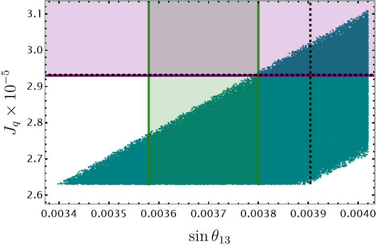
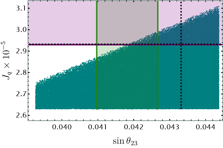
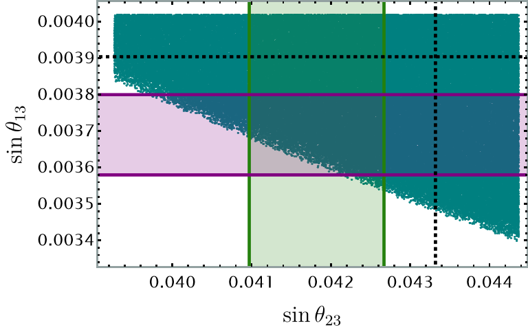
Figure 1: Correlation plot between the mixing angles of the quarks and the Jarlskog invariant obtained with our model. The green and purple bands represent the $1\sigma$ range in the experimental values, while the dotted line (black) represents the best-fit point by our model.

IV Lepton masses and mixings

IV.1 Charged lepton sector

The $Z_{4}^{\prime}$ charge assignments of the model fields shown in the table 1, as well the VEV pattern of the $S_{4}$ scalar triplets $S_{e}$, $S_{\mu}$ and $S_{\tau}$ shown in Eq. (11) imply that the charged lepton Yukawa terms of (II), yield a diagonal charged lepton mass matrix:

$$M_{l}=\left(\begin{array}[]{ccc}m_{e}&0&0\\ 0&m_{\mu}&0\\ 0&0&m_{\tau}\end{array}\right),$$ (31)

Where the masses of the SM charged leptons are given by:

$$m_{e}=y_{1}^{\left(L\right)}\frac{v_{S_{e}}v_{\rho}}{\Lambda}=a_{1}\frac{v_{\rho}}{\Lambda},\hskip 28.45274ptm_{\mu}=y_{2}^{\left(L\right)}\frac{v_{S_{\mu}}v_{\rho}}{\Lambda}=a_{2}\frac{v_{\rho}}{\Lambda},\hskip 28.45274ptm_{\tau}=y_{3}^{\left(L\right)}\frac{v_{S_{\tau}}v_{\rho}}{\Lambda}=a_{3}\frac{v_{\rho}}{\Lambda}$$ (32)

IV.2 Neutrino sector

The neutrino Yukawa interactions of Eq. (II) give rise to the following neutrino mass terms:

$$-\mathcal{L}_{mass}^{\left(\nu\right)}=\frac{1}{2}\left(\begin{array}[]{ccc}\overline{\nu_{L}^{C}}&\overline{\nu_{R}}&\overline{N_{R}}\end{array}\right)M_{\nu}\left(\begin{array}[]{c}\nu_{L}\\ \nu_{R}^{C}\\ N_{R}^{C}\end{array}\right)+H.c,$$ (33)

where the neutrino mass matrix reads:

$$M_{\nu}=\begin{pmatrix}0_{3\times 3}&m_{\nu_{D}}&0_{3\times 3}\\ m_{\nu_{D}}^{T}&0_{3\times 3}&M\\ 0_{3\times 3}&M^{T}&\mu\end{pmatrix},$$ (34)

and the submatrices are given by:

$$m_{\nu_{D}} = \frac{y_{\nu}v_{\rho}v_{\Phi}}{\sqrt{2}\Lambda}\left(\begin{array}[]{ccc}0&r_{1}e^{i\theta}&r_{1}e^{i\theta}\\ -r_{1}e^{i\theta}&0&1\\ -r_{1}e^{i\theta}&-1&0\end{array}\right),\hskip 28.45274pt\hskip 28.45274ptM=y_{\chi}^{\left(L\right)}\frac{v_{\chi}}{\sqrt{2}}\left(\begin{array}[]{ccc}1&0&0\\ 0&1&0\\ 0&0&1\end{array}\right),$$ (41)

$$\mu = \left(\begin{array}[]{ccc}h_{1N}v_{\varphi}&h_{2N}v_{\xi}r_{2}&h_{2N}v_{\xi}\\ h_{2N}v_{\xi}r_{2}&h_{1N}v_{\varphi}&h_{2N}v_{\xi}\\ h_{2N}v_{\xi}&h_{2N}v_{\xi}&h_{1N}v_{\varphi}\end{array}\right)\frac{v_{\sigma}^{2}}{\Lambda^{2}}.$$ (45)

The light active masses arise from an inverse seesaw mechanism and the resulting physical neutrino mass matrices take the form:

$$\widetilde{M}_{\nu} = m_{\nu_{D}}\left(M^{T}\right)^{-1}\mu M^{-1}m_{\nu_{D}}^{T},$$ (46)

$$\widetilde{M}_{\nu}^{(1)} = \frac{1}{2}\mu-\frac{1}{2}\left(M+M^{T}\right),$$ (47)

$$\widetilde{M}_{\nu}^{(2)} = \frac{1}{2}\mu+\frac{1}{2}\left(M+M^{T}\right).$$ (48)

Here, $\widetilde{M}_{\nu}$ is the mass matrix for the active neutrino ($\nu_{\alpha}$), whereas $\widetilde{M}_{\nu}^{(1)}$ and $\widetilde{M}_{\nu}^{(2)}$ are the sterile neutrinos mass matrices.
Thus, the light active neutrino mass matrix is given by:

$$\widetilde{M}_{\nu}=\left(\begin{array}[]{ccc}2a^{2}\left(y_{2}+z\right)&a\left(b\left(y_{2}+z\right)-a\left(y_{1}+y_{2}\right)\right)&-a\left(a\left(y_{1}+y_{2}\right)+b\left(y_{2}+z\right)\right)\\ a\left(b\left(y_{2}+z\right)-a\left(y_{1}+y_{2}\right)\right)&z\left(a^{2}+b^{2}\right)-2aby_{2}&a^{2}z+ab\left(y_{1}-y_{2}\right)-b^{2}y_{2}\\ -a\left(a\left(y_{1}+y_{2}\right)+b\left(y_{2}+z\right)\right)&a^{2}z+ab\left(y_{1}-y_{2}\right)-b^{2}y_{2}&z\left(a^{2}+b^{2}\right)+2aby_{1}\\ \end{array}\right),$$ (49)

where:

$$a =\frac{y_{\nu}v_{\rho}v_{\Phi}r_{1}}{y_{\chi}^{(L)}v_{\chi}\Lambda}e^{i\theta}, b =\frac{y_{\nu}v_{\rho}v_{\Phi}}{y_{\chi}^{(L)}v_{\chi}\Lambda}, y_{1} =\frac{v_{\sigma}^{2}h_{2N}v_{\xi}r_{2}}{\Lambda^{2}},$$

$$y_{2} =\frac{v_{\sigma}^{2}h_{2N}v_{\xi}}{\Lambda^{2}}, z =\frac{v_{\sigma}^{2}h_{1N}v_{\varphi}}{\Lambda^{2}}.$$ (50)

If we considering the parameter $b$ as pure imaginary, we obtain a cobimaximal texture for the mass matrix of the light-active neutrinos in the equation. (49) and adapting the function $\chi^{2}$ from Eq. (29) for the neutrino sector observables, we obtain the following error function:

$$\chi^{2}=\frac{\left(m_{21}^{\exp}-m_{21}^{th}\right)^{2}}{\sigma_{m_{21}}^{2}}+\frac{\left(m_{31}^{\exp}-m_{31}^{th}\right)^{2}}{\sigma_{m_{31}}^{2}}+\frac{\left(s_{\theta_{12}}^{\exp}-s_{\theta_{12}}^{th}\right)^{2}}{\sigma_{s_{12}}^{2}}+\frac{\left(s_{\theta_{23}}^{\exp}-s_{\theta_{23}}^{th}\right)^{2}}{\sigma_{s_{23}}^{2}}+\frac{\left(s_{\theta_{13}}^{\exp}-s_{\theta_{13}}^{th}\right)^{2}}{\sigma_{s_{13}}^{2}}+\frac{\left(\delta_{CP}^{\exp}-\delta_{CP}^{th}\right)^{2}}{\sigma_{\delta}^{2}}\;,$$ (51)

which allows us to adjust the parameters of the model. Therefore, after minimizing Eq. (51), we get the following values for the model parameters:

$$a =0.5208e^{-3.027i}, b =1.080i, y_{1} =-0.08645,\;\text{eV}^{2}$$

$$y_{2} =2.053,\;\text{eV}^{2} z =-2.300,\;\text{eV}^{2}$$ (52)

The diagonalization of the matrix (49) gives us the following eigenvalues:

$$m_{1}^{2} = 0,$$ (53)

$$m_{2}^{2} = \left(a^{2}\left(y_{2}+2z\right)+ab\left(y_{1}-y_{2}\right)+b^{2}z\right.$$ (54)

$$-\left.\sqrt{2a^{2}y_{1}^{2}\left(a^{2}+b^{2}\right)+2ay_{2}y_{1}(a-b)\left(2a^{2}+ab+b^{2}\right)+y_{2}^{2}\left(a^{2}+b^{2}\right)\left(3a^{2}+2ab+b^{2}\right)}\right)^{2},$$

$$m_{3}^{2} = \left(a^{2}\left(y_{2}+2z\right)+ab\left(y_{1}-y_{2}\right)+b^{2}z\right.$$ (55)

$$+\left.\sqrt{2a^{2}y_{1}^{2}\left(a^{2}+b^{2}\right)+2ay_{2}y_{1}(a-b)\left(2a^{2}+ab+b^{2}\right)+y_{2}^{2}\left(a^{2}+b^{2}\right)\left(3a^{2}+2ab+b^{2}\right)}\right)^{2}.$$

With the values of the parameters of our best-fit point of the equation (52), we obtain the results of the neutrino sector that are shown in the table 4, together with the experimental values in the range of $3\sigma$, whose experimental data were taken from deSalas:2020pgw . In the 4 table, we can see that all the values obtained by our model of the neutrino oscillation range from $1\sigma$ to $3\sigma$.

Observable	range	$\Delta m_{21}^{2}$ [$10^{-5}$eV2]	$\Delta m_{31}^{2}$ [$10^{-3}$eV2]	$\sin\theta^{(l)}_{12}/10^{-1}$	$\sin\theta^{(l)}_{13}/10^{-3}$	$\sin\theta^{(l)}_{23}/10^{-1}$	$\delta^{(l)}_{CP}(^{\circ})$
Experimental	$1\sigma$	$7.50_{-0.20}^{+0.22}$	$2.55_{-0.03}^{+0.02}$	$3.18\pm 0.16$	$2.200_{-0.062}^{+0.069}$	$5.74\pm 0.14$	$194_{-22}^{+24}$
Value	$3\sigma$	$6.94-8.14$	$2.47-2.63$	$2.71-3.69$	$2.000-2.405$	$4.34-6.10$	$128-359$
Fit	$1\sigma-3\sigma$	$7.498$	$2.541$	$3.024$	$2.191$	$5.931$	$246.4$

Table 4: Model predictions for the scenario of normal order (NO) neutrino mass. The experimental values are taken from Ref. deSalas:2020pgw

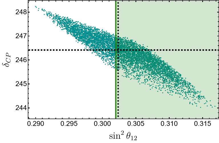
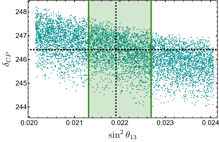
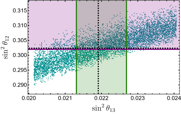
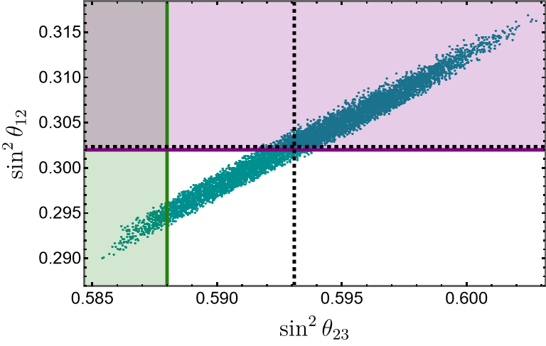
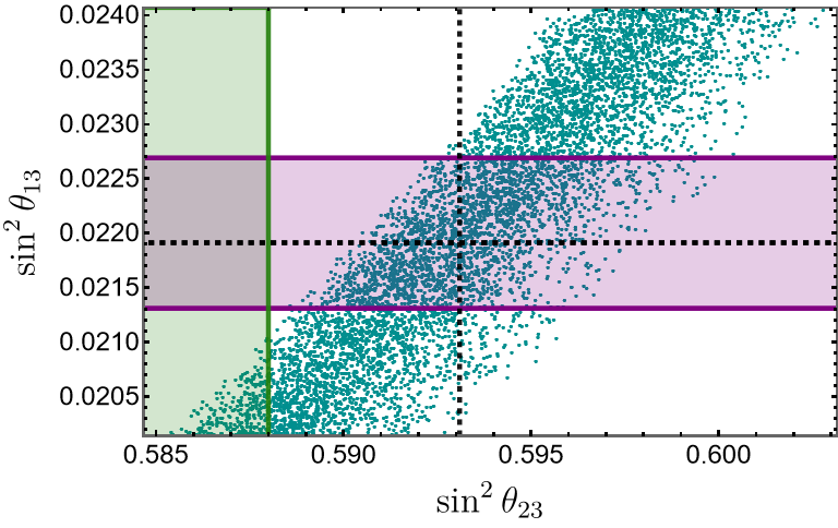
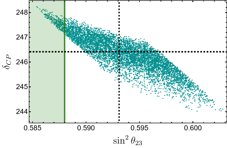
Figure 2: Correlation between the mixing angles of the neutrino sector and the CP violation phase obtained with our model. The green and purple bands represent the $1\sigma$ range in the experimental values, while the dotted line (black) represents the best-fit point of our model.

Fig. 2 shows the correlation between the leptonic Dirac CP violating phase and the neutrino mixing angles as well as the correlations among the leptonic mixing angles, where the green and purple background fringes represent the $1\sigma$ range of the experimental values and the black bands the dotted lines represent our best-fit point for each observable. In Fig. 2, we see that for the mixing angles, we can get values in the $1\sigma$ range, while for the CP violating phase, we obtain values up to $3\sigma$, where each lepton sector observable is obtained in the following range of values: $0.290\leq\sin^{2}\theta_{12}\leq 0.317$, $0.0201\leq\sin^{2}\theta_{13}\leq 0.0241$, $0.584\leq\sin^{2}\theta_{23}\leq 0.603$ and $244^{\circ}\leq\delta_{CP}\leq 248^{\circ}$.

V Scalar potential for the $SU(3)_{L}$ triplets.

The most general renormalizable potential invariant under $S_{4}$ which we can write with the four triplets of the Eqs. (II) is given by

$$V = -\mu_{\chi}^{2}(\chi^{\dagger}\chi)+\mu_{\eta_{1}}^{2}\eta_{1}^{\dagger}\eta_{1}-\mu_{\eta_{2}}^{2}\eta_{2}^{\dagger}\eta_{2}-\mu_{\rho}^{2}(\rho^{\dagger}\rho)+A\eta_{2}\rho\chi+\lambda_{1}(\chi^{\dagger}\chi)(\chi^{\dagger}\chi)+\lambda_{2}(\eta^{\dagger}\eta)_{\mathbf{1}}(\eta^{\dagger}\eta)_{\mathbf{1}}$$

$$+\lambda_{3}(\eta^{\dagger}\eta)_{\mathbf{1}^{\prime}}(\eta^{\dagger}\eta)_{\mathbf{1}^{\prime}}+\lambda_{4}(\eta^{\dagger}\eta)_{\mathbf{2}}(\eta^{\dagger}\eta)_{\mathbf{2}}+\lambda_{5}(\eta^{\dagger}\eta)_{\mathbf{1}}(\chi^{\dagger}\chi)+\lambda_{6}\left[(\eta^{\dagger}\chi)(\chi^{\dagger}\eta)\right]_{\mathbf{1}}$$

$$+\lambda_{7}(\rho^{\dagger}\rho)^{2}+\lambda_{8}(\eta^{\dagger}\eta)_{\mathbf{1}}(\rho^{\dagger}\rho)+\lambda_{9}(\chi^{\dagger}\chi)(\rho^{\dagger}\rho)+h.c$$

where $\eta_{1}$ is an inert $SU(3)_{L}$ scalar triplet, the $\mu$’s are mass parameters and $A$ is the trilinear scalar coupling, while $\lambda$’s are the quartic dimensionless couplings. Furthermore, the minimization conditions of the scalar potential yield the following relations

$$\mu_{\chi}^{2} = -\frac{A}{\sqrt{2}}\frac{v_{\eta_{2}}v_{\rho}}{v_{\chi}}+\frac{\lambda_{5}}{2}v_{\eta_{2}}^{2}+\frac{\lambda_{9}}{2}v_{\rho}^{2}+\lambda_{1}v_{\chi}^{2},$$

$$\mu_{\eta_{2}}^{2} = -\frac{A}{\sqrt{2}}\frac{v_{\rho}v_{\chi}}{v_{\eta_{2}}}+\frac{\lambda_{8}}{2}v_{\rho}^{2}+\frac{\lambda_{5}}{2}v_{\chi}^{2}+\left(\lambda_{2}+\lambda_{4}\right)v_{\eta_{2}}^{2},$$ (57)

$$\mu_{\rho}^{2} = -\frac{A}{\sqrt{2}}\frac{v_{\eta_{2}}v_{\chi}}{v_{\rho}}+\frac{\lambda_{8}}{2}v_{\eta_{2}}^{2}+\frac{\lambda_{9}}{2}v_{\chi}^{2}+\lambda_{7}v_{\rho}^{2}.$$

After spontaneous symmetry breaking, the Higgs mass spectrum comes from the diagonalization of the squared mass matrices (see appendix B). The mixing angles for the physical eigenstates are:

$$\tan\alpha = \frac{v_{\eta_{2}}}{v_{\chi}},\quad\tan\beta\ =\ \frac{v_{\rho}}{v_{\chi}},\quad\tan\tau\ =\ \frac{v_{\eta_{2}}}{v_{\rho}},\quad\tan\delta=\frac{v_{\chi}}{v_{\rho}\sin\tau},\quad\tan 2\vartheta=\frac{2\sqrt{2}\lambda_{8}}{Av_{\chi}}\frac{v_{\eta_{2}}^{2}v_{\rho}^{2}}{v_{\rho}^{2}-v_{\eta_{2}}^{2}},$$ (58)

the figure 3, presents correlation plots demonstrating the relationships between mixing angles and physical scalar masses. These plots highlight specific correlations, such as the correlation between the $\tau$ angle and charged fields, and the correlation between the $\delta$ angle and charged and pseudo-scalar fields. These correlations provide invaluable insights into the interactions among scalar fields and enhance our understanding of particle properties and the relationships between their masses and mixing angles. Moreover, similar correlations were observed for other mixing angles. The correlation analyses of the mixing angles offer valuable information regarding the underlying theoretical structure and relationships within the model.

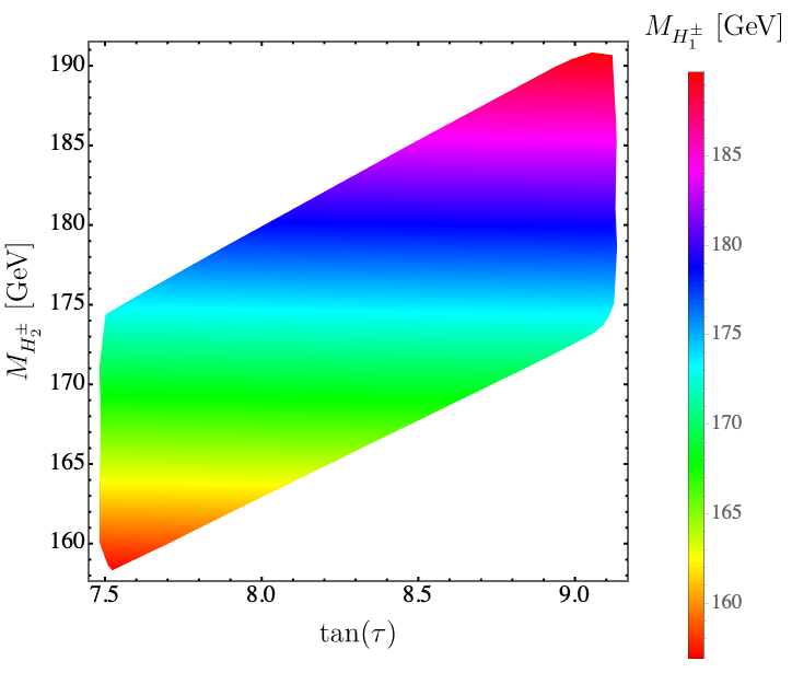
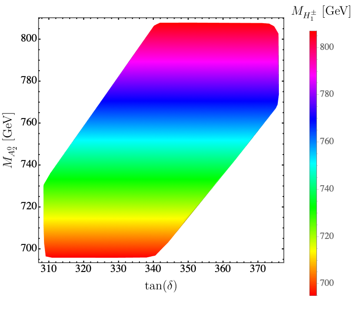
Figure 3: Correlations between mixing angles and the masses of the physical charged scalar, neutral scalar/pseudoscalar fields.

We find that the charged sector is composed of two Goldstone bosons and three massive charged scalars.

$$M_{G_{1}^{\pm}}^{2} = M_{G_{2}^{\pm}}^{2}=0,$$ (59)

$$M_{H_{1}^{\pm}}^{2} = \frac{Av_{\eta_{2}}v_{\rho}}{\sqrt{2}v_{\chi}}+\frac{A_{2}v_{\eta_{2}}v_{\chi}}{\sqrt{2}v_{\rho}},$$ (60)

$$M_{H_{2}^{\pm}}^{2} = \frac{Av_{\eta_{2}}v_{\chi}}{\sqrt{2}v_{\rho}}+\frac{Av_{\rho}v_{\chi}}{\sqrt{2}v_{\eta_{2}}},$$ (61)

$$M_{H_{3}^{\pm}}^{2} = \mu_{\eta_{1}}^{2}+\left(\lambda_{2}-\lambda_{4}\right)v_{\eta_{2}}^{2}+\frac{\lambda_{8}v_{\rho}^{2}}{2}+\frac{\lambda_{5}v_{\chi}^{2}}{2}.$$ (62)

The Goldstone bosons come only from mixing between $\rho_{3}^{\pm}$ and $\eta_{22}^{\pm}$, through the angle $\tau$, while $\chi_{2}^{\pm}$ is a massive field charged, the other two bulk fields correspond to the blending of $\rho_{1}^{\pm}$ and the charged component of the scalar intert $\eta_{21}^{\pm}$ by blending angle $\beta$, i.e,

$$\begin{array}[]{lll}G_{1}^{\pm}=\cos\tau\ \rho_{3}^{\pm}-\sin\tau\ \eta_{22}^{\pm},&&G_{2}^{\pm}=\sin\tau\ \rho_{3}^{\pm}+\cos\tau\ \eta_{22}^{\pm},\\ H_{1}^{\pm}=\cos\beta\ \rho_{1}^{\pm}-\sin\beta\ \eta_{21}^{\pm},&&H_{2}^{\pm}=\sin\beta\ \rho_{1}^{\pm}+\cos\beta\ \eta_{21}^{\pm},\\ H_{3}^{\pm}=\chi_{2}^{\pm}.&&\end{array}$$ (63)

The physical mass eigenvalues of the CP odd scalars $A_{1}^{0},\ A_{2}^{0}$ and the Goldstone bosons $G_{1}^{0},\ G_{2}^{0}$ can be written as:

$$M_{G_{1}^{0}}^{2} = M_{G_{2}^{0}}^{2}\ =\ 0,$$ (64)

$$M_{A_{1}^{0}}^{2} = \frac{Av_{\eta_{2}}v_{\rho}}{\sqrt{2}v_{\chi}}+\frac{A}{\sqrt{2}}\left(v_{\eta_{2}}^{2}+v_{\rho}^{2}\right)v_{\chi}^{2},$$ (65)

$$M_{A_{2}^{0}}^{2} = \mu_{\eta_{1}}^{2}+v_{\eta_{2}}^{2}\left(\lambda_{2}-2\lambda_{3}-\lambda_{4}\right)+\frac{\lambda_{8}v_{\rho}^{2}}{2}+\frac{\lambda_{5}v_{\chi}^{2}}{2}.$$ (66)

We have the following relationship between the original physical eigenstates:

$$\begin{array}[]{lll}G_{1}^{0}=\cos\tau\ \zeta_{\rho}-\cos\delta\cos\tau\ \zeta_{\eta_{1}}-\sin\tau\ \zeta_{\eta_{2}},&&G_{2}^{0}=\cos\delta\ \zeta_{\rho}+\sin\delta\ \zeta_{\eta_{1}},\\ A_{1}^{0}=\sin\tau\ \zeta_{\rho}-\cos\delta\sin\tau\ \zeta_{\eta_{1}}+\cos\tau\ \zeta_{\eta_{2}},&&A_{2}^{0}=\zeta_{\chi},\end{array}$$ (67)

where consider the following limit $v_{\chi}\gg v_{\rho},v_{\eta_{2}}$.

The masses of the light and heavy eigenstates for CP even scalars are given as:

$$M^{2}_{h} = A\frac{\left(v_{\eta_{2}}^{2}+v_{\rho}^{2}\right)v_{\chi}}{2\sqrt{2}v_{\eta_{2}}v_{\rho}}-\frac{1}{2\sqrt{2}v_{\eta_{2}}v_{\rho}}\sqrt{A^{2}\left(v_{\eta_{2}}^{2}-v_{\rho}^{2}\right)^{2}v_{\chi}^{2}+8\lambda_{8}v_{\eta_{2}}^{4}v_{\rho}^{4}},$$ (68)

$$M_{H_{1}^{0}} = A\frac{\left(v_{\eta_{2}}^{2}+v_{\rho}^{2}\right)v_{\chi}}{2\sqrt{2}v_{\eta_{2}}v_{\rho}}+\frac{1}{2\sqrt{2}v_{\eta_{2}}v_{\rho}}\sqrt{A^{2}\left(v_{\eta_{2}}^{2}-v_{\rho}^{2}\right)^{2}v_{\chi}^{2}+8\lambda_{8}v_{\eta_{2}}^{4}v_{\rho}^{4}},$$ (69)

$$M_{H_{2}^{0}} = \mu_{\eta_{1}}^{2}+\left(\lambda_{2}+\lambda_{4}\right)v_{\eta_{2}}^{2}+\frac{\lambda_{8}}{2}v_{\rho}^{2}+\frac{\lambda_{5}}{2}v_{\chi}^{2},$$ (70)

$$M_{H_{3}^{0}} = 2\lambda_{1}v_{\chi}^{2}.$$ (71)

The lighter mass eigenstate $h$ is identified as the SM Higgs boson. The two mass eigenstates $h$ and $H_{1}^{0}$ are related with the $\xi_{\eta_{2}}$ and $\xi_{\rho}$ fields through the rotation angle $\vartheta$ as:

$$h \simeq \xi_{\eta_{2}}\cos\vartheta-\xi_{\rho}\sin\vartheta,$$ (72)

$$H_{1}^{0} \simeq \xi_{\eta_{2}}\sin\vartheta+\xi_{\rho}\cos\vartheta,$$ (73)

while the heavier fields are related as $H_{2}^{0}\simeq\xi_{\eta_{1}}$ and $H_{3}^{0}\simeq\xi_{\chi}$.

Finally, for the pseudoscalar and scalar neutral complex fields, we have composed the mixture of the Imaginary and Real parts of $\eta_{31}^{0},\ \eta_{32}^{0},\ \chi_{1}^{0}$, respectively,

$$M_{G_{3}^{0}}^{2} = M_{G_{4}^{0}}^{2}\ =\ 0$$ (74)

$$M_{A_{3}^{0}}^{2} = \sqrt{2}A\left(\frac{v_{\eta_{2}}v_{\rho}}{v_{\chi}}+\frac{v_{\rho}v_{\chi}}{v_{\eta_{2}}}\right)-\lambda_{6}\left(v_{\chi}^{2}+v_{\eta_{2}}^{2}\right)$$ (75)

$$M_{A_{4}^{0}}^{2} = 2\mu_{\eta_{1}}^{2}+2\left(\lambda_{2}-\lambda_{4}\right)v_{\eta_{2}}^{2}+\lambda_{8}v_{\rho}^{2}+\left(\lambda_{5}-\lambda_{6}\right)v^{2}_{\chi}$$ (76)

$$M_{H_{4}^{0}}^{2} = \sqrt{2}A\left(\frac{v_{\eta_{2}}v_{\rho}}{v_{\chi}}+\frac{v_{\rho}v_{\chi}}{v_{\eta_{2}}}\right)+\lambda_{6}\left(v_{\chi}^{2}+v_{\eta_{2}}^{2}\right)$$ (77)

$$M_{H_{5}^{0}}^{2} = 2\mu_{\eta_{1}}^{2}+2\left(\lambda_{2}-\lambda_{4}\right)v_{\eta_{2}}^{2}+\lambda_{8}v_{\rho}^{2}+\left(\lambda_{5}+\lambda_{6}\right)v_{\chi}^{2}$$ (78)

In the physical eigenstates, there are two Goldstone bosons and one pseudoscalar massive boson, and a scalar from the mixture of the complex neutral part of $\eta_{1}$ and $\eta_{2}$, while,

$$\begin{array}[]{lll}G_{3}^{0}=\sin\alpha\ \text{Im}\eta_{31}^{0}-\cos\alpha\ \text{Im}\eta_{32}^{0},&&G_{4}^{0}=-\sin\alpha\ \text{Re}\eta_{31}^{0}+\cos\alpha\ \text{Re}\eta_{32}^{0},\\ A_{3}^{0}=\cos\alpha\ \text{Im}\eta_{31}^{0}+\sin\alpha\ \text{Im}\eta_{32}^{0},&&H_{4}^{0}=\cos\alpha\ \text{Re}\eta_{31}^{0}+\sin\alpha\ \text{Re}\eta_{32}^{0},\\ A_{4}^{0}=\text{Im}\chi_{1}^{0},&&H_{5}^{0}=\text{Re}\chi_{1}^{0}.\end{array}$$ (79)

In our model for the physical scalar spectrum, the light scalar field $h$, is identified as the SM-like Higgs boson, additionally six charged fields $\left(H_{1}^{\pm},H_{2}^{\pm},H_{3}^{\pm}\right)$, four CP even $\left(H_{1}^{0},H_{2}^{0},H_{3}^{0},H_{4}^{0},H_{5}^{0}\right)$ and three CP odd fields $\left(A_{1}^{0},A_{2}^{0},A_{3}^{0},A_{4}^{0}\right)$, in figure 4, corresponds to cases of the correlation between the charged and neutral scalar masses, figure 4 (a), shows a linear correlation between of the masses between the charged field and the pseudoscalar neutral field, $H_{1}^{\pm}$ and $A_{1}^{0}$ respectively, in figure 4 (b), a linear correlation between the masses of the pseudoscalar and scalar neutral field, $A_{3}^{0}$ and $H_{3}^{0}$ respectively. The charged Goldstone bosons $\left(G_{1}^{\pm},G_{2}^{\pm}\right)$ are related to the longitudinal components of the $W^{\pm}$ and $W^{\prime\pm}$ gauge bosons respectively; while the neutral Goldstone bosons $\left(G_{1}^{0},G_{2}^{0},G_{3}^{0},G_{4}^{0}\right)$ are associated to the longitudinal components of the $Z$, $Z^{\prime}$, $K^{0}$ and $K^{\prime 0}$ gauge bosons. Our best fit point that allows to successfully accommodate the $125$ GeV mass for the SM like Higgs boson found at the LHC corresponds to the following VEV values:

$$v_{\chi}\simeq 9.994\ \text{TeV},\quad v_{\rho}\simeq 29.54\ \text{GeV},\quad v_{\eta_{2}}\simeq 244.2\ \text{GeV}$$ (80)

which yield a mass of $m_{h}=125.387\ \text{GeV}$ for the SM like Higgs boson. However, to determine the specific benchmark that reproduces the $125$ GeV mass value for the SM-like Higgs boson, the numerical values of the relevant parameters in the model are required. With the adjustment of these parameters, the numerical contributions of the physical spectrum can be determined. These parameters are necessary for accommodating phenomenological processes that arise in this model and provide more precise determinations of phenomena such as K meson oscillations. In the SM-type two-photon Higgs decay constraints, where extra-charged scalar fields induce one loop level corrections to the Higgs diphoton decay. At the same time, the oblique corrections are affected by the presence of extra scalar fields. These phenomenological processes are studied in more detail in the following sections.

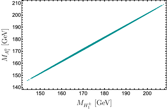
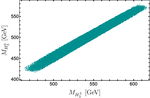
Figure 4: Correlation plot between the pseudoscalar neutral, scalar neutral, and scalar charged masses.

VI Meson mixings

In this section we discuss the implications of our model in the Flavour Changing Neutral Current (FCNC) interactions in the down type quark sector. These FCNC down type quark Yukawa interactions produce $K^{0}-\bar{K}^{0}$, $B_{d}^{0}-\bar{B}_{d}^{0}$ and $B_{s}^{0}-\bar{B}_{s}^{0}$ meson oscillations, whose corresponding effective Hamiltonians are:

$$\mathcal{H}_{eff}^{\left(K\right)}\mathcal{=}\sum_{j=1}^{3}\kappa_{j}^{\left(K\right)}\left(\mu\right)\mathcal{O}_{j}^{\left(K\right)}\left(\mu\right),$$ (81)

$$\mathcal{H}_{eff}^{\left(B_{d}\right)}\mathcal{=}\sum_{j=1}^{3}\kappa_{j}^{\left(B_{d}\right)}\left(\mu\right)\mathcal{O}_{j}^{\left(B_{d}\right)}\left(\mu\right),$$ (82)

$$\mathcal{H}_{eff}^{\left(B_{s}\right)}\mathcal{=}\sum_{j=1}^{3}\kappa_{j}^{\left(B_{s}\right)}\left(\mu\right)\mathcal{O}_{j}^{\left(B_{s}\right)}\left(\mu\right),$$ (83)

where:

$$\mathcal{O}_{1}^{\left(K\right)} = \left(\overline{s}_{R}d_{L}\right)\left(\overline{s}_{R}d_{L}\right),\hskip 19.91684pt\hskip 19.91684pt\mathcal{O}_{2}^{\left(K\right)}=\left(\overline{s}_{L}d_{R}\right)\left(\overline{s}_{L}d_{R}\right),\hskip 19.91684pt\hskip 19.91684pt\mathcal{O}_{3}^{\left(K\right)}=\left(\overline{s}_{R}d_{L}\right)\left(\overline{s}_{L}d_{R}\right),$$ (84)

$$\mathcal{O}_{1}^{\left(B_{d}\right)} = \left(\overline{d}_{R}b_{L}\right)\left(\overline{d}_{R}b_{L}\right),\hskip 19.91684pt\hskip 19.91684pt\mathcal{O}_{2}^{\left(B_{d}\right)}=\left(\overline{d}_{L}b_{R}\right)\left(\overline{d}_{L}b_{R}\right),\hskip 19.91684pt\hskip 19.91684pt\mathcal{O}_{3}^{\left(B_{d}\right)}=\left(\overline{d}_{R}b_{L}\right)\left(\overline{d}_{L}b_{R}\right),$$ (85)

$$\mathcal{O}_{1}^{\left(B_{s}\right)} = \left(\overline{s}_{R}b_{L}\right)\left(\overline{s}_{R}b_{L}\right),\hskip 19.91684pt\hskip 19.91684pt\mathcal{O}_{2}^{\left(B_{s}\right)}=\left(\overline{s}_{L}b_{R}\right)\left(\overline{s}_{L}b_{R}\right),\hskip 19.91684pt\hskip 19.91684pt\mathcal{O}_{3}^{\left(B_{s}\right)}=\left(\overline{s}_{R}b_{L}\right)\left(\overline{s}_{L}b_{R}\right),$$ (86)

and the Wilson coefficients take the form:

$$\kappa_{1}^{\left(K\right)} = \frac{x_{h\overline{s}_{R}d_{L}}^{2}}{m_{h}^{2}}+\sum_{m=1}^{5}\sum_{n=1}^{4}\left(\frac{x_{H_{m}^{0}\overline{s}_{R}d_{L}}^{2}}{m_{H_{m}^{0}}^{2}}-\frac{x_{A_{n}^{0}\overline{s}_{R}d_{L}}^{2}}{m_{A_{n}^{0}}^{2}},\right)$$ (87)

$$\kappa_{2}^{\left(K\right)} = \frac{x_{h\overline{s}_{L}d_{R}}^{2}}{m_{h}^{2}}+\sum_{m=1}^{5}\sum_{n=1}^{4}\left(\frac{x_{H_{m}^{0}\overline{s}_{L}d_{R}}^{2}}{m_{H_{m}^{0}}^{2}}-\frac{x_{A_{n}^{0}\overline{s}_{L}d_{R}}^{2}}{m_{A_{n}^{0}}^{2}}\right),\hskip 19.91684pt\hskip 19.91684pt$$ (88)

$$\kappa_{3}^{\left(K\right)} = \frac{x_{h\overline{s}_{R}d_{L}}x_{h\overline{s}_{L}d_{R}}}{m_{h}^{2}}+\sum_{m=1}^{5}\sum_{n=1}^{4}\left(\frac{x_{H_{m}^{0}\overline{s}_{R}d_{L}}x_{H_{m}^{0}\overline{s}_{L}d_{R}}}{m_{H_{m}^{0}}^{2}}-\frac{x_{A_{n}^{0}\overline{s}_{R}d_{L}}x_{A_{n}^{0}\overline{s}_{L}d_{R}}}{m_{A_{n}^{0}}^{2}}\right),$$ (89)

$$\kappa_{1}^{\left(B_{d}\right)} = \frac{x_{h\overline{d}_{R}b_{L}}^{2}}{m_{h}^{2}}+\sum_{m=1}^{5}\sum_{n=1}^{4}\left(\frac{x_{H_{m}^{0}\overline{d}_{R}b_{L}}^{2}}{m_{H_{m}^{0}}^{2}}-\frac{x_{A_{n}^{0}\overline{d}_{R}b_{L}}^{2}}{m_{A_{n}^{0}}^{2}}\right),$$ (90)

$$\kappa_{2}^{\left(B_{d}\right)} = \frac{x_{h\overline{d}_{L}b_{R}}^{2}}{m_{h}^{2}}+\sum_{m=1}^{5}\sum_{n=1}^{4}\left(\frac{x_{H_{m}^{0}\overline{d}_{L}b_{R}}^{2}}{m_{H_{m}^{0}}^{2}}-\frac{x_{A_{n}^{0}\overline{d}_{L}b_{R}}^{2}}{m_{A_{n}^{0}}^{2}}\right),$$ (91)

$$\kappa_{3}^{\left(B_{d}\right)} = \frac{x_{h\overline{d}_{R}b_{L}}x_{h\overline{d}_{L}b_{R}}}{m_{h}^{2}}+\sum_{m=1}^{5}\sum_{n=1}^{4}\left(\frac{x_{H_{m}^{0}\overline{d}_{R}b_{L}}x_{H_{m}^{0}\overline{d}_{L}b_{R}}}{m_{H_{m}^{0}}^{2}}-\frac{x_{A_{n}^{0}\overline{d}_{R}b_{L}}x_{A_{n}^{0}\overline{d}_{L}b_{R}}}{m_{A_{n}^{0}}^{2}}\right),$$ (92)

$$\kappa_{1}^{\left(B_{s}\right)} = \frac{x_{h\overline{s}_{R}b_{L}}^{2}}{m_{h}^{2}}+\sum_{m=1}^{5}\sum_{n=1}^{4}\left(\frac{x_{H_{m}^{0}\overline{s}_{R}b_{L}}^{2}}{m_{H_{m}^{0}}^{2}}-\frac{x_{A_{n}^{0}\overline{s}_{R}b_{L}}^{2}}{m_{A_{n}^{0}}^{2}}\right),$$ (93)

$$\kappa_{2}^{\left(B_{s}\right)} = \frac{x_{h\overline{s}_{L}b_{R}}^{2}}{m_{h}^{2}}+\sum_{m=1}^{5}\sum_{n=1}^{4}\left(\frac{x_{H_{m}^{0}\overline{s}_{L}b_{R}}^{2}}{m_{H_{m}^{0}}^{2}}-\frac{x_{A_{n}^{0}\overline{s}_{L}b_{R}}^{2}}{m_{A_{n}^{0}}^{2}}\right),$$ (94)

$$\kappa_{3}^{\left(B_{s}\right)} = \frac{x_{h\overline{s}_{R}b_{L}}x_{h\overline{s}_{L}b_{R}}}{m_{h}^{2}}+\sum_{m=1}^{5}\sum_{n=1}^{4}\left(\frac{x_{H_{m}^{0}\overline{s}_{R}b_{L}}x_{H_{m}^{0}\overline{s}_{L}b_{R}}}{m_{H_{m}^{0}}^{2}}-\frac{x_{A_{n}^{0}\overline{s}_{R}b_{L}}x_{A_{n}^{0}\overline{s}_{L}b_{R}}}{m_{A_{n}^{0}}^{2}}\right),$$ (95)

where we have used the notation of section V for the physical scalars, assuming $h$ is the lightest of the CP-even ones and corresponds to the SM Higgs. The $K-\bar{K}$, $B_{d}^{0}-\bar{B}_{d}^{0}$ and $B_{s}^{0}-\bar{B}_{s}^{0}$ meson mass splittings read:

$$\Delta m_{K}=\Delta m_{K}^{\left(SM\right)}+\Delta m_{K}^{\left(NP\right)},\hskip 28.45274pt\Delta m_{B_{d}}=\Delta m_{B_{d}}^{\left(SM\right)}+\Delta m_{B_{d}}^{\left(NP\right)},\hskip 28.45274pt\Delta m_{B_{s}}=\Delta m_{B_{s}}^{\left(SM\right)}+\Delta m_{B_{s}}^{\left(NP\right)},$$ (96)

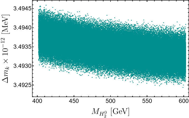
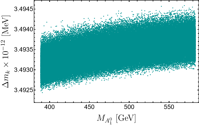
Figure 5: Correlation a) between the $\Delta m_{B_{k}}$ mass splitting and the lightest CP even scalar mass $m_{H_{2}^{0}}$, b) between the $\Delta m_{B_{k}}$ mass splitting and the lightest CP odd scalar mass $m_{A_{1}^{0}}$.

where $\Delta m_{K}^{\left(SM\right)}$, $\Delta m_{B_{d}}^{\left(SM\right)}$ and $\Delta m_{B_{s}}^{\left(SM\right)}$ correspond to the SM contributions, while $\Delta m_{K}^{\left(NP\right)}$, $\Delta m_{B_{d}}^{\left(NP\right)}$ and $\Delta m_{B_{s}}^{\left(NP\right)}$ are due to new physics effects. Our model predicts the following new physics contributions for the $K-\bar{K}$, $B_{d}^{0}-\bar{B}_{d}^{0}$ and $B_{s}^{0}-\bar{B}_{s}^{0}$ meson mass differences:

$$\Delta m_{K}^{\left(NP\right)} \simeq \frac{8}{3}f_{K}^{2}\eta_{K}B_{K}m_{K}\left[r_{2}^{\left(K\right)}\kappa_{3}^{\left(K\right)}+r_{1}^{\left(K\right)}\left(\kappa_{1}^{\left(K\right)}+\kappa_{2}^{\left(K\right)}\right)\right]\leavevmode\nobreak\ ,$$ (97)

$$\Delta m_{B_{d}}^{\left(NP\right)} \simeq \frac{8}{3}f_{B_{d}}^{2}\eta_{B_{d}}B_{B_{d}}m_{B_{d}}\left[r_{2}^{\left(B_{d}\right)}\kappa_{3}^{\left(B_{d}\right)}+r_{1}^{\left(B_{d}\right)}\left(\kappa_{1}^{\left(B_{d}\right)}+\kappa_{2}^{\left(B_{d}\right)}\right)\right]\leavevmode\nobreak\ ,$$ (98)

$$\Delta m_{B_{s}}^{\left(NP\right)} \simeq \frac{8}{3}f_{B_{s}}^{2}\eta_{B_{s}}B_{B_{s}}m_{B_{s}}\left[r_{2}^{\left(B_{s}\right)}\kappa_{3}^{\left(B_{s}\right)}+r_{1}^{\left(B_{s}\right)}\left(\kappa_{1}^{\left(B_{s}\right)}+\kappa_{2}^{\left(B_{s}\right)}\right)\right]\leavevmode\nobreak\ .$$ (99)

Since the contribution arising from the flavor changing down type quark interaction involving the $Z^{\prime}$ gauge boson exchange is very small and subleading, the main contributions to the meson mass differences is due to the virtual exchange of additional scalar and pseudosalar fields participating in the flavor violating Yukawa interactions of the model under consideration. Using the following numerical values of the meson parameters Dedes:2002er ; Aranda:2012bv ; Khalil:2013ixa ; Queiroz:2016gif ; Buras:2016dxz ; Ferreira:2017tvy ; NguyenTuan:2020xls :

$$\left(\Delta m_{K}\right)_{\exp} = \left(3.484\pm 0.006\right)\times 10^{-12}\,\mathrm{{MeV},\hskip 42.67912pt\left(\Delta m_{K}\right)_{SM}=3.483\times 10^{-12}\,{MeV}}$$

$$f_{K} = 155.7\,\mathrm{{MeV},\hskip 42.67912ptB_{K}=0.85,\hskip 42.67912pt\eta_{K}=0.57,}$$

$$r_{1}^{\left(K\right)} = -9.3,\hskip 42.67912ptr_{2}^{\left(K\right)}=30.6,\hskip 42.67912ptm_{K}=\left(497.611\pm 0.013\right)\,\mathrm{{MeV},}$$ (100)

$$\left(\Delta m_{B_{d}}\right)_{\exp} = \left(3.334\pm 0.013\right)\times 10^{-10}\,\mathrm{{MeV},\hskip 42.67912pt\left(\Delta m_{B_{d}}\right)_{SM}=\left(3.653\pm 0.037\pm 0.019\right)\times 10^{-10}\,{MeV},}$$

$$f_{B_{d}} = 188\,\mathrm{{MeV},\hskip 42.67912ptB_{B_{d}}=1.26,\hskip 42.67912pt\eta_{B_{d}}=0.55,}$$

$$r_{1}^{\left(B_{d}\right)} = -0.52,\hskip 42.67912ptr_{2}^{\left(B_{d}\right)}=0.88,\hskip 42.67912ptm_{B_{d}}=\left(5279.65\pm 0.12\right)\,\mathrm{{MeV},}$$ (101)

$$\left(\Delta m_{B_{s}}\right)_{\exp} = \left(1.1683\pm 0.0013\right)\times 10^{-8}\,\mathrm{{MeV},\hskip 42.67912pt\left(\Delta m_{B_{s}}\right)_{SM}=\left(1.1577\pm 0.022\pm 0.051\right)\times 10^{-8}\,{MeV},}$$

$$f_{B_{s}} = 225\,\mathrm{{MeV},\hskip 42.67912ptB_{B_{s}}=1.33,\hskip 42.67912pt\eta_{B_{s}}=0.55,}$$

$$r_{1}^{\left(B_{s}\right)} = -0.52,\hskip 42.67912ptr_{2}^{\left(B_{s}\right)}=0.88,\hskip 42.67912ptm_{B_{s}}=\left(5366.9\pm 0.12\right)\,\mathrm{{MeV},}$$ (102)

Fig. 5 (a) and Fig. 5 (b) show the correlations of the mass splitting $\Delta m_{B_{k}}$ with the mass of the lightest CP-even and CP-odd scale $m_{H_{2}^{0}}$ and $m_{A_{1}^{0}}$, respectively. In our numerical analysis, for the sake of simplicity, we have set the couplings of flavor-changing Yukawa neutral interactions that produce $(K^{0}-\overline{K}^{0})$ mixings to be equal to $10^{-6}$. In addition, we have varied the masses around 20% of their best fit-point values obtained in the analysis of the scalar sector shown in the plots of Fig. 4. As indicated in Fig. 5, our model can successfully accommodate the experimental constraints arising from $(K^{0}-\overline{K}^{0})$ meson oscillations for the above specified range of parameter space. We have numerically verified that in the range of masses described above, the values obtained for the mass splittings $\Delta m_{B_{d}}$ and $\Delta m_{B_{s}}$ are consistent with the experimental data on meson oscillations for flavor violating Yukawa couplings equal to $10^{-4}$ and $2.5\times 10^{-4}$, respectively.

VII Higgs di-photon decay rate

In order to study the implications of our model in the decay of the $125\ \mathrm{GeV}$ Higgs into a photon pair, one introduces the Higgs diphoton signal strength $R_{\gamma\gamma}$, which is defined as Bhattacharyya:2014oka :

$$R_{\gamma\gamma}=\frac{\sigma(pp\rightarrow h)\Gamma(h\rightarrow\gamma\gamma)}{\sigma(pp\rightarrow h)_{\text{SM}}\Gamma(h\rightarrow\gamma\gamma)_{\text{SM}}}\simeq a_{htt}^{2}\frac{\Gamma(h\rightarrow\gamma\gamma)}{\Gamma(h\rightarrow\gamma\gamma)_{\text{SM}}}.$$ (103)

That Higgs diphoton signal strength, normalizes the $\gamma\gamma$ signal predicted by our model in relation to the one given by the SM. Here we have used the fact that in our model, single Higgs production is also dominated by gluon fusion as in the Standard Model. In the 3-3-1 model $\sigma\left(pp\rightarrow h\right)=a_{htt}^{2}\sigma\left(pp\rightarrow h\right)_{\text{SM}}$, so $R_{\gamma\gamma}$ reduces to the ratio of branching ratios.
The decay rate for the $h\rightarrow\gamma\gamma$ process takes the form Bhattacharyya:2014oka ; Logan:2014jla ; Hernandez:2021uxx :

$$\Gamma(h\rightarrow\gamma\gamma)=\frac{\alpha_{\text{em}}^{2}m_{h}^{3}}{256\pi^{3}v^{2}}\left|\sum_{f}a_{hff}N_{C}Q_{f}^{2}F_{1/2}\left(\varrho_{f}\right)+a_{hWW}F_{1}\left(\varrho_{W}\right)+\sum_{k}\frac{C_{hH_{k}^{\pm}H_{k}^{\mp}}v}{2m_{H_{k}^{\pm}}^{2}}F_{0}\left(\varrho_{H_{k}^{\pm}}\right)\right|^{2}$$ (104)

where $\alpha_{\text{em}}$ is the fine structure constant, $N_{C}$ is the color factor ($N_{C}=3$ for quarks and $N_{C}=1$ for leptons) and $Q_{f}$ is the electric charge of the fermion in the loop. From the fermion-loop contributions we only consider the dominant top quark term. The $\varrho_{i}$ are the mass ratios $\varrho_{i}=4M_{i}^{2}/m_{h}^{2}$ with $M_{i}=m_{f},M_{W},M_{H_{k}^{\pm}}$ with $k=1,2,3$. Furthermore, $C_{hH_{k}^{\pm}H_{k}^{\mp}}$ is the trilinear coupling between the SM-like Higgs and a pair of charged Higges, whereas $a_{htt}$ and $a_{hWW}$ are the deviation factors from the SM Higgs-top quark coupling and the SM Higgs-W gauge boson coupling, respectively (in the SM these factors are unity). Such deviation factors are close to unity in our model, which is a consequence of the numerical analysis of its scalar, Yukawa and gauge sectors.

The form factors for the contributions from spin-$0$, $1/2$ and $1$ particles are:

$$F_{0}(\varrho) = -\varrho(1-\varrho f(\varrho)),$$ (105)

$$F_{1/2}(\varrho) = 2\varrho(1+(1-\varrho)f(\varrho)),$$ (106)

$$F_{1}(\varrho) = -\left(2+3\varrho+3\varrho\left(2-\varrho\right)f(\varrho)\right),$$ (107)

with

$$f(\varrho)=\begin{cases}\arcsin^{2}\sqrt{\varrho^{-1}}&\text{ for }\varrho\geq 1\\ -\frac{1}{4}\left[\ln\left(\frac{1+\sqrt{1-\varrho}}{1-\sqrt{1-\varrho}}\right)-i\pi\right]^{2}&\text{ for }\varrho<1\end{cases}$$ (108)

Table 5 displays the best-fit values of the $R_{\gamma\gamma}$ ratio in comparison to the best-fit signals measured in CMS 10.1007/978-981-19-2354-8_33 and ATLAS ATLAS:2022tnm . In this analysis, the charged fields play a key role in determining the value of the ratio, while the other fields have an indirect impact through the parameter space involving the VEV (vacuum expectation values) and the trilinear scalar coupling $A$, as well as some $\lambda_{i}$. From our numerical analysis, it follows that our model favors a Higgs diphoton decay rate lower than the SM expectation but inside the $3\sigma$ experimentally allowed range. The correlation of the Higgs diphoton signal strength with the charged scalar mass $M_{H_{2}^{\pm}}$ is shown in Fig. 6, which indicates that our model successfully accommodates the current Higgs diphoton decay rate constraints. Additionally, it should be noted that the correlation with $M_{H_{1}^{\pm}}$ is similar; however, the correlation is weaker than for $M_{H_{3}^{\pm}}$.

	Model value	CMS	ATLAS
$R_{\gamma\gamma}$	$0.982\pm 0.08$	$1.02_{-0.09}^{+0.11}$	$1.04_{-0.09}^{+0.10}$

Table 5: The best fit for the ratio of Higgs boson diphoton decay obtained from the model indicates a lower Higgs decay rate into two photons compared to the expectation of the Standard Model in ATLAS ATLAS:2022tnm and CMS 10.1007/978-981-19-2354-8_33 collaboration. However, this value still falls within the $3\sigma$ experimentally allowed range.

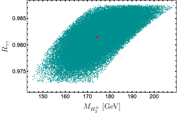
Figure 6: Correlation of the Higgs di-photon signal strength with the charged scalar mass. The red star point corresponds to the best fit for $R_{\gamma\gamma}$ (see Table 5).

VIII Oblique $T$, $S$ and $U$ parameters

The parameters $S$, $T$, and $U$ basically quantify the corrections to the two-point functions of gauge bosons through loop diagrams. In our case, where there are three $SU(3)_{L}$ scalar triplets that introduce new scalar particles, which lead to new Higgs-mediated contributions to the self-energies of gauge bosons through loop diagrams. Based on references Peskin:1991sw ; Altarelli:1990zd ; Barbieri:2004qk , the parameters $S$, $T$, and $U$ can be defined as follows:

$$T = \frac{1}{\alpha_{\text{em}}M_{W}}\left.\left[\Pi_{11}\left(q^{2}\right)-\Pi_{33}\left(q^{2}\right)\right]\right|_{q=0}$$ (109)

$$S = -\left.\frac{4c_{W}s_{W}}{\alpha_{\text{em}}}\frac{d}{dq^{2}}\Pi_{30}\left(q^{2}\right)\right|_{q^{2}=0},$$ (110)

$$U = \frac{4s_{W}}{\alpha_{\text{em}}}\left.\frac{d}{dq^{2}}\left[\Pi_{11}\left(q^{2}\right)-\Pi_{33}\left(q^{2}\right)\right]\right|_{q^{2}=0},$$ (111)

with $s_{W}=\sin\theta_{W}$ and $c_{W}=\cos\theta_{W}$, where $\theta_{W}$ is the electroweak mixing angle, the quantity $\Pi_{ij}\left(q\right)$ is defined in terms of the vacuum-polarization tensors

$$\Pi_{ij}^{\mu\nu}\left(q^{2}\right)=g^{\mu\nu}\Pi_{ij}\left(q^{2}\right)-iq^{\mu}q^{\nu}\Delta_{ij}\left(q^{2}\right),$$ (112)

where $i,j=0,1,3$ for the $B$, $W_{1}$ and $W_{3}$ bosons respectively, or possibly $i,j=W,Z,\gamma$. If the new physics enters at the TeV scale, the effect of the theory will be well-described by an expansion up to linear order in $q^{2}$ for $\Pi_{ij}\left(q^{2}\right)$ as presented in reference Peskin:1991sw .

For our 331 model, the scalar fields directly contribute to the new physics values of the $T$, $S$, and $U$ oblique parameters, and we must take into account the scalar mixing angles. We can calculate the parameters considering that the low energy effective field theory below the scale of spontaneos breaking of the $SU(3)_{L}\times U(1)_{X}\times U(1)_{L_{g}}$ symmetry corresponds to a three Higgs doublet model (3HDM), where the three Higgs doublets arise from the $\eta_{1}$, $\eta_{2}$ and $\rho$ $SU(3)_{L}$ scalar triplets. Then, following these considerations, in the above described low energy limit scenario, the leading contributions to the oblique $T$, $S$ and $U$ parameters take the form Long:1999bny ; Long:2018dun ; CarcamoHernandez:2022vjk ; Batra:2022arl :

$$T \simeq t_{0}\left[\sum_{a=1}^{2}\sum_{k=1}^{2}\left[\left(R_{C}\right)_{ak}\right]^{2}m_{H_{k}^{\pm}}^{2}+\sum_{a=1}^{2}\sum_{i=1}^{2}\sum_{j=1}^{2}\left[\left(R_{H}\right)_{ai}\left(R_{A}\right)_{aj}\right]^{2}F\left(m_{H_{i}^{0}}^{2},m_{A_{j}^{0}}^{2}\right)\right.,$$

$$\left.-\sum_{a=1}^{2}\sum_{i=1}^{2}\sum_{k=1}^{2}\left\{\left[\left(R_{H}\right)_{ai}\left(R_{C}\right)_{ak}\right]^{2}F\left(m_{H_{i}^{0}}^{2},m_{H_{k}^{\pm}}^{2}\right)+\left[\left(R_{A}\right)_{ai}\left(R_{C}\right)_{ak}\right]^{2}F\left(m_{A_{i}^{0}}^{2},m_{H_{k}^{\pm}}^{2}\right)\right\}\right]$$

$$S \simeq \frac{1}{12\pi}\sum_{i=1}^{2}\sum_{j=1}^{2}\sum_{k=1}^{2}\left[\left(R_{H}\right)_{ki}\left(R_{A}\right)_{kj}\right]^{2}K\left(m_{H_{i}^{0}}^{2},m_{A_{j}^{0}}^{2},m_{H_{k}^{\pm}}^{2}\right),$$ (114)

$$U \simeq -S+\sum_{a=1}^{2}\sum_{i=1}^{2}\sum_{k=1}^{2}\left\{\left[\left(R_{A}\right)_{ai}\left(R_{C}\right)_{ak}\right]^{2}G\left(m_{A_{i}^{0}}^{2},m_{H_{k}^{\pm}}^{2}\right)+\left[\left(R_{H}\right)_{ai}\left(R_{C}\right)_{ak}\right]^{2}G\left(m_{H_{i}^{0}}^{2},m_{H_{k}^{\pm}}^{2}\right)\right\},$$ (115)

where $t_{0}=\left(16\pi^{2}v^{2}\alpha_{\text{em}}\left(M_{Z}\right)\right)^{-1}$ and $R_{C}$, $R_{H}$, $R_{A}$ are the mixing matrices for the charged scalar fields, neutral scalar and pseudoscalars, respectively presented in the Sec. V. Furthermore, the following loop functions $F\left(m_{1}^{2},m_{2}^{2}\right)$, $G\left(m_{1}^{2},m_{2}^{2}\right)$ and $K\left(m_{1}^{2},m_{2}^{2},m_{3}^{2}\right)$ were introduced in CarcamoHernandez:2022vjk :

$$F\left(m_{1}^{2},m_{2}^{2}\right) = \frac{m_{1}^{2}m_{2}^{2}}{m_{1}^{2}-m_{2}^{2}}\ln\left(\frac{m_{1}^{2}}{m_{2}^{2}}\right),$$ (116)

$$G\left(m_{1}^{2},m_{2}^{2}\right) = \frac{-5m_{1}^{6}+27m_{1}^{4}m_{2}^{2}-27m_{1}^{2}m_{2}^{4}+6\left(m_{1}^{6}-3m_{1}^{4}m_{2}^{2}\right)\ln\left(\frac{m_{1}^{2}}{m_{2}^{2}}\right)+5m_{2}^{6}}{6\left(m_{1}^{2}-m_{2}^{2}\right)^{3}},$$ (117)

$$K\left(m_{1}^{2},m_{2}^{2},m_{3}^{2}\right) = \frac{1}{\left(m_{2}^{2}-m_{1}^{2}\right)^{3}}\left\{m_{1}^{4}\left(3m_{2}^{2}-m_{1}^{2}\right)\ln\left(\frac{m_{1}^{2}}{m_{3}^{2}}\right)-m_{2}^{4}\left(3m_{1}^{2}-m_{2}^{2}\right)\ln\left(\frac{m_{2}^{2}}{m_{3}^{2}}\right)\right.$$

$$\left.-\frac{1}{6}\left[27m_{1}^{2}m_{2}^{2}\left(m_{1}^{2}-m_{2}^{2}\right)+5\left(m_{2}^{6}-m_{1}^{6}\right)\right]\right\}.$$

Besides that, the experimental limits for $S$, $T$, and $U$ are given in ref Workman:2022ynf :

$$T_{\text{exp}} = 0.03\pm 0.12$$ (119)

$$S_{\text{exp}} = -0.02\pm 0.1$$ (120)

$$U_{\text{exp}} = 0.01\pm 0.11$$ (121)

From the numerical analysis, the $S_{4}$ flavored $331$ model has restricted parameters because the determination of the new physics from $S$, $T$, and $U$ is determined by the physical masses of the model, also within the limit indicated by the oblique parameters present some correlation shown in figure 7, we see that the evolution of parameter space is adjusted within the $1\sigma$ experimental range, which corresponds to the overlying region. The figures 7 (a) and (c) of dispersion involving the $U$ parameter is produced with values larger than the central one, despite this, the values of $U$ fit within the range of $1\sigma$ and the statistical discrepancy is minimal. In the case of the $S$ value, due to the large uncertainty value, the value fits more naturally, as shown in the figure 7 (b).

Our analysis shows that our model allows a successfull fit for the oblique $S$, $T$ and $U$ parameters, consistent with their current experimental limits. The obtained best fit point values for the oblique $S$, $T$ and $U$ parameters in our model are:

$$T = 0.029\pm 0.009,$$ (122)

$$S = -0.016\pm 0.006,$$ (123)

$$U = 0.14\pm 0.04$$ (124)

Our results also suggest that the model favors a larger value for $U$ within statistical uncertainty. While the values for $S$ and $T$ fit within the relative error $0.2$ and $0.1$, respectively.

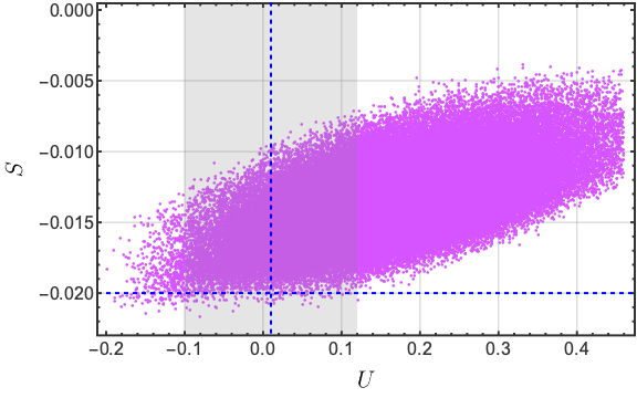
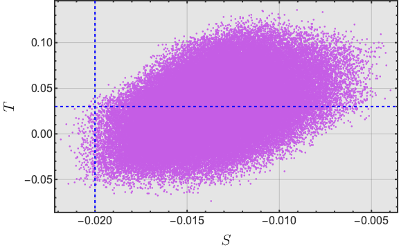
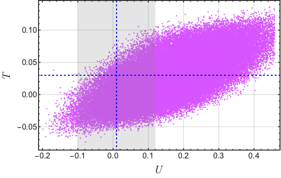
Figure 7: Correlation between the oblique parameters, the shaded region represents the measured values at $1\sigma$, while the dashed line represents the central value of the ref. Workman:2022ynf

IX Conclusions

We have constructed a 3-3-1 model where the $SU(3)_{C}\times SU(3)_{L}\times U(1)_{X}$ symmetry is enlarged by the inclusion of the spontaneously broken $U(1)_{L_{g}}\times S_{4}\times Z_{4}\times Z_{4}^{\prime}\times Z_{2}$ symmetry group. In our theory under consideration, the observed SM charged fermion mass hierarchy and the quark mixing pattern arise from the spontaneous breaking of discrete symmetries and the tiny active neutrino masses are generated from an inverse seesaw mechanism. Our proposed model leads to a successful fit to quark and lepton masses, mixing angles, and CP phases, whose obtained values are consistent with the experimental data within the $3\sigma$ range. The symmetries of the model give rise to correlations between the mixing angles and the Jarlskog invariant for the quark sector. Regarding the lepton sector, our model predicts a diagonal SM charged lepton mass matrix, thus implying that the leptonic mixing only arises from the neutrino sector, where correlations between the leptonic mixing angles and the leptonic CP violating phase are obtained. In addition, flavor-changing neutral current interactions in the quark sector mediated by CP even and odd CP scalars give rise to meson oscillations, such as the $(K^{0}-\overline{K}^{0})$ mixing, whose experimental constraints are successfully satisfied for an appropriate region of the parameter space. The theory under consideration is consistent with the masses and mixings of SM fermions as well as with the constraints arising from $(K^{0}-\overline{K}^{0})$ and $(B_{d,s}^{0}-\overline{B}_{d,s}^{0})$ meson oscillations. The charged scalars of our model provide the new physics contribution to the Higgs diphoton decay rate. In contrast, the rest of the scalar fields have an indirect influence involving the VEVs and the trilinear scalar coupling $A$, where our model favors a $R_{\gamma\gamma}$ value lower than SM, however, is within the $3\sigma$ experimentally allowed range measured by the CMS and ATLAS collaborations. The extra scalar fields of our model produce radiative corrections to the oblique parameters $S$, $T$, and $U$, where the numerical analysis yield correlations between these parameters and, in addition, their obtained values are within the $1\sigma$ experimentally allowed range.

Appendix A The product rules of the $S_{4}$ discrete group

The $S_{4}$ is the smallest non abelian group having doublet, triplet and singlet irreducible representations. $S_{4}$ is the group of permutations of four objects, which includes five irreducible representations, i.e., $\mathbf{1,1^{\prime},2,3,3^{\prime}}$ fulfilling the following tensor product rules Ishimori:2010au :

$$\begin{gathered}\mathbf{3}\otimes\mathbf{3}=\mathbf{1}\oplus\mathbf{2}\oplus\mathbf{3}\oplus\mathbf{3}^{\prime},\quad\mathbf{3}^{\prime}\otimes\mathbf{3}^{\prime}=\mathbf{1}\oplus\mathbf{2}\oplus\mathbf{3}\oplus\mathbf{3}^{\prime},\quad\mathbf{3}\otimes\mathbf{3}^{\prime}=\mathbf{1}^{\prime}\oplus\mathbf{2}\oplus\mathbf{3}\oplus\mathbf{3}^{\prime},\\ \mathbf{2}\otimes\mathbf{2}=\mathbf{1}\oplus\mathbf{1}^{\prime}\oplus\mathbf{2},\quad\mathbf{2}\otimes\mathbf{3}=\mathbf{3}\oplus\mathbf{3}^{\prime},\quad\mathbf{2}\otimes\mathbf{3}^{\prime}=\mathbf{3}^{\prime}\oplus\mathbf{3}\\ \mathbf{3}\otimes\mathbf{1}^{\prime}=\mathbf{3}^{\prime},\quad\mathbf{3}^{\prime}\otimes\mathbf{1}^{\prime}=\mathbf{3},\quad\mathbf{2}\otimes\mathbf{1}^{\prime}=\mathbf{2}\end{gathered}$$

Explicitly, the basis used in this paper corresponds to Ref. Ishimori:2010au and results in

$$\begin{pmatrix}a_{1}\\ a_{2}\\ a_{3}\end{pmatrix}_{\mathbf{3}}\otimes\begin{pmatrix}b_{1}\\ b_{2}\\ b_{3}\end{pmatrix}_{\mathbf{3}} = (a_{1}b_{1}+a_{2}b_{2}+a_{3}b_{3})_{\mathbf{1}_{1}}\oplus\begin{pmatrix}\frac{1}{\sqrt{2}}(a_{2}b_{2}-a_{3}b_{3})\\ \frac{1}{\sqrt{6}}(-2a_{1}b_{1}+a_{2}b_{2}+a_{3}b_{3})\end{pmatrix}_{\mathbf{2}}$$ (125)

$$\oplus\begin{pmatrix}a_{2}b_{3}+a_{3}b_{2}\\ a_{1}b_{3}+a_{3}b_{1}\\ a_{1}b_{2}+a_{2}b_{1}\end{pmatrix}_{\mathbf{3}}\oplus\begin{pmatrix}a_{3}b_{2}-a_{2}b_{3}\\ a_{1}b_{3}-a_{3}b_{1}\\ a_{2}b_{1}-a_{1}b_{2}\end{pmatrix}_{\mathbf{3^{\prime}}\ ,}$$

$$\begin{pmatrix}a_{1}\\ a_{2}\\ a_{3}\end{pmatrix}_{\mathbf{3^{\prime}}}\otimes\begin{pmatrix}b_{1}\\ b_{2}\\ b_{3}\end{pmatrix}_{\mathbf{3^{\prime}}} = (a_{1}b_{1}+a_{2}b_{2}+a_{3}b_{3})_{\mathbf{1}_{1}}\oplus\begin{pmatrix}\frac{1}{\sqrt{2}}(a_{2}b_{2}-a_{3}b_{3})\\ \frac{1}{\sqrt{6}}(-2a_{1}b_{1}+a_{2}b_{2}+a_{3}b_{3})\end{pmatrix}_{\mathbf{2}}$$ (126)

$$\oplus\begin{pmatrix}a_{2}b_{3}+a_{3}b_{2}\\ a_{1}b_{3}+a_{3}b_{1}\\ a_{1}b_{2}+a_{2}b_{1}\end{pmatrix}_{\mathbf{3}}\oplus\begin{pmatrix}a_{3}b_{2}-a_{2}b_{3}\\ a_{1}b_{3}-a_{3}b_{1}\\ a_{2}b_{1}-a_{1}b_{2}\end{pmatrix}_{\mathbf{3^{\prime}}\ ,}$$

$$\begin{pmatrix}a_{1}\\ a_{2}\\ a_{3}\end{pmatrix}_{\mathbf{3}}\otimes\begin{pmatrix}b_{1}\\ b_{2}\\ b_{3}\end{pmatrix}_{\mathbf{3^{\prime}}} = (a_{1}b_{1}+a_{2}b_{2}+a_{3}b_{3})_{\mathbf{1}_{2}}\oplus\begin{pmatrix}\frac{1}{\sqrt{6}}(2a_{1}b_{1}-a_{2}b_{2}-a_{3}b_{3})\\ \frac{1}{\sqrt{2}}(a_{2}b_{2}-a_{3}b_{3})\end{pmatrix}_{\mathbf{2}}$$ (127)

$$\oplus\begin{pmatrix}a_{3}b_{2}-a_{2}b_{3}\\ a_{1}b_{3}-a_{3}b_{1}\\ a_{2}b_{1}-a_{1}b_{2}\end{pmatrix}_{\mathbf{3}}\oplus\begin{pmatrix}a_{2}b_{3}+a_{3}b_{2}\\ a_{1}b_{3}+a_{3}b_{1}\\ a_{1}b_{2}+a_{2}b_{1}\end{pmatrix}_{\mathbf{3^{\prime}}\ .}$$

$$\begin{pmatrix}a_{1}\\ a_{2}\end{pmatrix}_{\mathbf{2}}\otimes\begin{pmatrix}b_{1}\\ b_{2}\end{pmatrix}_{\mathbf{2}} = (a_{1}b_{1}+a_{2}b_{2})_{\mathbf{1}}\oplus(-a_{1}b_{2}+a_{2}b_{1})_{\mathbf{1^{\prime}}}\oplus\begin{pmatrix}a_{1}b_{2}+a_{2}b_{1}\\ a_{1}b_{1}-a_{2}b_{2}\end{pmatrix}_{\mathbf{2}\ ,}$$ (128)

$$\begin{pmatrix}a_{1}\\ a_{2}\end{pmatrix}_{\mathbf{2}}\otimes\begin{pmatrix}b_{1}\\ b_{2}\\ b_{3}\end{pmatrix}_{\mathbf{3}} = \begin{pmatrix}a_{2}b_{1}\\ -\frac{1}{2}(\sqrt{3}a_{1}b_{2}+a_{2}b_{2})\\ \frac{1}{2}(\sqrt{3}a_{1}b_{3}-a_{2}b_{3})\end{pmatrix}_{\mathbf{3}}\oplus\begin{pmatrix}a_{1}b_{1}\\ \frac{1}{2}(\sqrt{3}a_{2}b_{2}-a_{1}b_{2})\\ -\frac{1}{2}(\sqrt{3}a_{2}b_{3}+a_{1}b_{3})\end{pmatrix}_{\mathbf{3^{\prime}}\ ,}$$ (129)

$$\begin{pmatrix}a_{1}\\ a_{2}\end{pmatrix}_{\mathbf{2}}\otimes\begin{pmatrix}b_{1}\\ b_{2}\\ b_{3}\end{pmatrix}_{\mathbf{3^{\prime}}} = \begin{pmatrix}a_{1}b_{1}\\ \frac{1}{2}(\sqrt{3}a_{2}b_{2}-a_{1}b_{2})\\ -\frac{1}{2}(\sqrt{3}a_{2}b_{3}+a_{1}b_{3})\end{pmatrix}_{\mathbf{3}}\oplus\begin{pmatrix}a_{2}b_{1}\\ -\frac{1}{2}(\sqrt{3}a_{1}b_{2}+a_{2}b_{2})\\ \frac{1}{2}(\sqrt{3}a_{1}b_{3}-a_{2}b_{3})\end{pmatrix}_{\mathbf{3^{\prime}}\ ,}$$ (130)

Appendix B Mass squared mastrices for scalar sector

In the de Born level analysis of the mass spectrum of the Higgs bosons and the physical basis of scalar particles, we must construct the scalar mass matrices of the model. Then substituting the equations of constraintst (57), and Eq.(II) into the scalar potential Eq.(V), the square mass matrices are determined, calculating the second derivatives of the potential

$$\left(M^{2}_{\phi^{\pm}}\right)_{ij}=\left.\frac{\partial V}{\partial\phi^{+}_{i}\partial\phi_{j}^{-}}\right|_{\left\langle\phi^{\pm}\right\rangle},\quad\quad\left(M^{2}_{\phi}\right)_{ij}=\left.\frac{\partial V}{\partial\phi_{i}\partial\phi_{j}}\right|_{\left\langle\phi\right\rangle},$$ (131)

where $\phi^{\pm}=\chi_{2}^{+},\rho_{1}^{+},\rho_{3}^{+},\eta_{21}^{+},\eta_{22}^{+},\chi_{2}^{-},\rho_{1}^{-},\rho_{3}^{-},\eta_{21}^{-},\eta_{22}^{-}$, for chaged fields and $\phi=$ $\xi_{\chi},\xi_{\rho},\xi_{\eta_{1}},\xi_{\eta_{2}},\zeta_{\chi},$ $\zeta_{\rho},$ $\zeta_{\eta_{1}},$ $\zeta_{\eta_{2}},$ $\chi_{1}^{0},\eta_{31}^{0},\eta_{32}^{0}$, for neutral scalar fields. Due to the symmetry of our models, the matrices of the CP odd and CP even sectors contain two diagonal blocks, a situation similar to that presented in other works on 3-3-1 models CarcamoHernandez:2019iwh , however, our results differ in higher dimension matrices due to the extra intert field.

In the charged sector, we can obtain a mass squared matrix in the basis $\left(\eta_{21}^{\pm},\eta_{22}^{\pm},\rho_{1}^{\pm},\rho_{3}^{\pm},\chi_{2}^{\pm}\right)$ of the form.

$$M^{2}_{\phi^{\pm}}=\left(\begin{array}[]{ccccc}\mu_{\eta_{1}}^{2}+\left(\lambda-\lambda_{4}\right)v_{\eta}^{2}+\frac{\lambda_{8}}{2}v_{\rho}^{2}+\frac{\lambda_{5}}{2}v_{\chi}^{2}&0&0&0&0\\ 0&\frac{Av_{\rho}v_{\chi}}{\sqrt{2}v_{\eta_{2}}}&\frac{Av_{\chi}}{\sqrt{2}}&0&0\\ 0&\frac{Av_{\chi}}{\sqrt{2}}&\frac{Av_{\chi}v_{\eta_{2}}}{\sqrt{2}v_{\rho}}&0&0\\ 0&0&0&\frac{Av_{\chi}v_{\eta_{2}}}{\sqrt{2}v_{\rho}}&\frac{Av_{\eta_{2}}}{\sqrt{2}}\\ 0&0&0&\frac{Av_{\eta_{2}}}{\sqrt{2}}&\frac{Av_{\rho}v_{\eta_{2}}}{\sqrt{2}v_{\chi}}\\ \end{array}\right)$$ (132)

In sector CP odd, the square matrices in the pseudoscalar neutral basis $\left(\zeta_{\eta_{1}},\zeta_{\eta_{2}},\zeta_{\rho},\zeta_{\chi}\right)$

$$M^{2}_{\zeta}=\left(\begin{array}[]{cccc}\mu_{\eta_{1}}^{2}+\left(\lambda_{2}-2\lambda_{3}-\lambda_{4}\right)v_{\eta_{2}}^{2}+\frac{\lambda_{8}}{2}v_{\rho}^{2}+\frac{\lambda_{5}}{2}v_{\chi}^{2}&0&0&0\\ 0&\frac{Av_{\rho}v_{\chi}}{\sqrt{2}v_{\eta_{2}}}&\frac{Av_{\chi}}{\sqrt{2}}&\frac{Av_{\rho}}{\sqrt{2}}\\ 0&\frac{Av_{\chi}}{\sqrt{2}}&\frac{Av_{\chi}v_{\eta_{2}}}{\sqrt{2}v_{\rho}}&\frac{Av_{\eta_{2}}}{\sqrt{2}}\\ 0&\frac{Av_{\rho}}{\sqrt{2}}&\frac{Av_{\eta_{2}}}{\sqrt{2}}&\frac{Av_{\rho}v_{\eta_{2}}}{\sqrt{2}v_{\chi}}\\ \end{array}\right)$$ (133)

and neutral scalar complex at the basis $\left(\text{Im}\eta_{31}^{0},\text{Im}\eta_{32}^{0},\text{Im}\chi_{1}^{0}\right)$

$$M_{\phi_{\text{Im}}}^{2}=\left(\begin{array}[]{ccc}2\mu_{\eta_{1}}^{2}+2\left(\lambda_{2}-\lambda_{4}\right)v_{\eta_{2}}^{2}+\lambda_{8}v_{\rho}^{2}+\left(\lambda_{5}-\lambda_{6}\right)v_{\chi}^{2}&0&0\\ 0&\frac{\sqrt{2}Av_{\rho}v_{\chi}}{v_{\eta_{2}}}-\lambda_{6}v_{\chi}^{2}&\lambda_{6}v_{\eta_{2}}v_{\chi}-\sqrt{2}Av_{\rho}\\ 0&\lambda_{6}v_{\eta_{2}}v_{\chi}-\sqrt{2}Av_{\rho}&\frac{\sqrt{2}Av_{\eta_{2}}v_{\rho}}{v_{\chi}}-\lambda_{6}v_{\eta_{2}}^{2}\\ \end{array}\right)$$ (134)

In the sector CP even, the square mass matrices in the scalar neutral basis $\left(\xi_{\eta_{1}},\xi_{\eta_{2}},\xi_{\rho},\xi_{\chi}\right)$

$$M^{2}_{\xi}=\left(\begin{array}[]{cccc}\mu_{\eta_{1}}^{2}+\left(\lambda_{2}+\lambda_{4}\right)v_{\eta_{2}}^{2}+\frac{\lambda_{8}}{2}v_{\rho}^{2}+\frac{\lambda_{5}}{2}v_{\chi}^{2}&0&0&0\\ 0&\frac{Av_{\rho}v_{\chi}}{\sqrt{2}v_{\eta_{2}}^{2}}+2\left(\lambda_{2}+\lambda_{4}\right)v_{\eta_{2}}^{2}&\lambda_{8}v_{\eta_{2}}v_{\rho}-\frac{Av_{\chi}}{\sqrt{2}}&\lambda_{5}v_{\eta_{2}}v_{\chi}-\frac{Av_{\rho}}{\sqrt{2}}\\ 0&\lambda_{8}v_{\eta_{2}}v_{\rho}-\frac{Av_{\chi}}{\sqrt{2}}&\frac{Av_{\eta_{2}}v_{\chi}}{\sqrt{2}v_{\rho}}+2\lambda_{7}v_{\rho}^{2}&\lambda_{9}v_{\rho}v_{\chi}-\frac{Av_{\eta_{2}}}{\sqrt{2}}\\ 0&\lambda_{5}v_{\eta_{2}}v_{\chi}-\frac{Av_{\rho}}{\sqrt{2}}&\lambda_{9}v_{\rho}v_{\chi}-\frac{Av_{\eta_{2}}}{\sqrt{2}}&\frac{Av_{\eta_{2}}v_{\rho}}{\sqrt{2}v_{\chi}}+2\lambda_{1}v_{\chi}^{2}\\ \end{array}\right)$$ (135)

and neutral scalar complex at the basis $\left(\text{Re}\eta_{31}^{0},\text{Re}\eta_{32}^{0},\text{Re}\chi_{1}^{0}\right)$

$$M_{\phi_{\text{Re}}}^{2}=\left(\begin{array}[]{ccc}2\mu_{\eta_{1}}^{2}+2\left(\lambda_{2}-\lambda_{4}\right)v_{\eta_{2}}^{2}+\lambda_{8}v_{\rho}^{2}+\left(\lambda_{5}+\lambda_{6}\right)v_{\chi}^{2}&0&0\\ 0&\frac{\sqrt{2}Av_{\rho}v_{\chi}}{v_{\eta_{2}}}+\lambda_{6}v_{\chi}^{2}&\sqrt{2}Av_{\rho}+\lambda_{6}v_{\eta_{2}}v_{\chi}\\ 0&\sqrt{2}Av_{\rho}+\lambda_{6}v_{\eta_{2}}v_{\chi}&\frac{\sqrt{2}Av_{\eta_{2}}v_{\rho}}{v_{\chi}}+\lambda_{6}v_{\eta_{2}}^{2}\\ \end{array}\right)$$ (136)

References

(1)
J. W. F. Valle and M. Singer, “Lepton Number Violation With Quasi Dirac
Neutrinos,”
Phys. Rev.D28 (1983) 540.
(15)
A. E. Cárcamo Hernández, S. Kovalenko, H. N. Long, and I. Schmidt, “A
variant of 3-3-1 model for the generation of the SM fermion mass and mixing
pattern,” JHEP07 (2018) 144,
arXiv:1705.09169 [hep-ph].
(18)
A. E. Cárcamo Hernández, N. A. Pérez-Julve, and Y. Hidalgo Velásquez,
“Fermion masses and mixings and some phenomenological aspects of a 3-3-1
model with linear seesaw mechanism,”
Phys. Rev.D100 no. 9, (2019) 095025,
arXiv:1907.13083 [hep-ph].
(19)
A. E. Cárcamo Hernández, D. T. Huong, and H. N. Long, “Minimal model for
the fermion flavor structure, mass hierarchy, dark matter, leptogenesis, and
the electron and muon anomalous magnetic moments,”
Phys. Rev. D102 no. 5, (2020) 055002,
arXiv:1910.12877
[hep-ph].
(21)
V. H. Binh, D. T. Binh, A. E. Cárcamo Hernández, D. T. Huong, D. V. Soa,
and H. N. Long, “Higgs sector phenomenology in the 3-3-1 model with axion
like particle,” arXiv:2007.05004 [hep-ph].
(23)
A. E. C. Hernández, C. Hati, S. Kovalenko, J. W. F. Valle, and C. A.
Vaquera-Araujo, “Scotogenic neutrino masses with gauged matter parity and
gauge coupling unification,”
JHEP03
(2022) 034, arXiv:2109.05029 [hep-ph].
(24)
P. N. Thu, N. T. Duy, A. E. Carcamo Hernandez, and D. T. Huong, “Lepton
universality violation in the MF331 model,”
arXiv:2304.03003
[hep-ph].
(25)
R. Mohapatra and J. W. F. Valle, “Neutrino Mass and Baryon Number
Nonconservation in Superstring Models,”
Phys.Rev.D34 (1986) 1642.
(26)
C. D. Froggatt and H. B. Nielsen, “Hierarchy of Quark Masses, Cabibbo Angles
and CP Violation,”
Nucl. Phys. B147 (1979) 277–298.
(27)
G. Altarelli, F. Feruglio, and L. Merlo, “Revisiting Bimaximal Neutrino
Mixing in a Model with S(4) Discrete Symmetry,”
JHEP05 (2009) 020, arXiv:0903.1940 [hep-ph].
(30)
R. de Adelhart Toorop, F. Bazzocchi, and L. Merlo, “The Interplay Between GUT
and Flavour Symmetries in a Pati-Salam x S4 Model,”
JHEP08
(2010) 001, arXiv:1003.4502
[hep-ph].
(37)
G.-J. Ding, S. F. King, C. Luhn, and A. J. Stuart, “Spontaneous CP violation
from vacuum alignment in models of leptons,”
JHEP05
(2013) 084, arXiv:1303.6180
[hep-ph].
(44)
F. J. de Anda, S. F. King, and E. Perdomo, “ grand unified theory of flavour and leptogenesis,”
JHEP12
(2017) 075, arXiv:1710.03229 [hep-ph]. [Erratum: JHEP 04, 069 (2019)].
(50)
J. D. García-Aguilar, A. E. P. Ramírez, M. M. S. Castañeda, and
J. C. Gómez-Izquierdo, “Soft breaking of the
symmetry by ,”
arXiv:2209.01316
[hep-ph].
(51)
A. E. Cárcamo Hernández, C. Espinoza, J. C. Gómez-Izquierdo, J. M.
González, and M. Mondragón, “Predictive extended 3HDM with family
symmetry,” arXiv:2212.12000 [hep-ph].
(54)Particle Data Group Collaboration, R. L. Workman and Others,
“Review of Particle Physics,”
PTEP2022
(2022) 083C01.
(55)
P. F. de Salas, D. V. Forero, S. Gariazzo, P. Martínez-Miravé, O. Mena,
C. A. Ternes, M. Tórtola, and J. W. F. Valle, “2020 global reassessment
of the neutrino oscillation picture,”
JHEP02
(2021) 071, arXiv:2006.11237 [hep-ph].
(61)
P. M. Ferreira, I. P. Ivanov, E. Jiménez, R. Pasechnik, and H. Serôdio,
“CP4 miracle: shaping Yukawa sector with CP symmetry of order four,”
JHEP01
(2018) 065, arXiv:1711.02042 [hep-ph].
(66)
P. Saha, “Recent measurements of higgs boson properties in the diphoton decay
channel with the cms detector,” in Proceedings of the XXIV DAE-BRNS
High Energy Physics Symposium, Jatni, India, B. Mohanty, S. K. Swain,
R. Singh, and V. K. S. Kashyap, eds., pp. 183–186.
Springer Nature Singapore, Singapore, 2022.
(67)ATLAS Collaboration, “Measurement of the properties of Higgs
boson production at TeV in the channel
using fb-1 of collision data with the ATLAS experiment,”
arXiv:2207.00348
[hep-ex].