DiffusionNER: Boundary Diffusion for Named Entity Recognition

Abstract

In this paper, we propose DiffusionNER, which formulates the named entity recognition task as a boundary-denoising diffusion process and thus generates named entities from noisy spans. During training, DiffusionNER gradually adds noises to the gold entity boundaries by a fixed forward diffusion process and learns a reverse diffusion process to recover the entity boundaries. In inference, DiffusionNER first randomly samples some noisy spans from a standard Gaussian distribution and then generates the named entities by denoising them with the learned reverse diffusion process. The proposed boundary-denoising diffusion process allows progressive refinement and dynamic sampling of entities, empowering DiffusionNER with efficient and flexible entity generation capability. Experiments on multiple flat and nested NER datasets demonstrate that DiffusionNER achieves comparable or even better performance than previous state-of-the-art models.

1 Introduction

Named Entity Recognition (NER) is a basic task of information extraction (Tjong Kim Sang and De Meulder, 2003), which aims to locate entity mentions and label specific entity types such as person, location, and organization. It is fundamental to many structured information extraction tasks, such as relation extraction (Li and Ji, 2014; Miwa and Bansal, 2016) and event extraction (McClosky et al., 2011; Wadden et al., 2019).

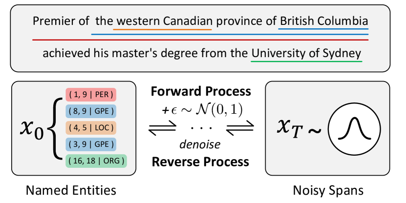
Figure 1: Boundary diffusion in named entity recognition. The fixed forward diffusion process adds Gaussian noise to the entity boundaries at each timestep, and the noisy boundaries recover original state by denoising with the learnable reverse diffusion process. For inference, the reverse diffusion process generates entity boundaries and performs entity typing based on the noisy spans sampled from the Gaussian distribution.

Most traditional methods (Chiu and Nichols, 2016) formulate the NER task into a sequence labeling task by assigning a single label to each token. To accommodate the nested structure between entities, some methods (Ju et al., 2018; Wang et al., 2020) further devise cascaded or stacked tagging strategies. Another class of methods treat NER as a classification task on text spans (Sohrab and Miwa, 2018; Eberts and Ulges, 2020), and assign labels to word pairs (Yu et al., 2020; Li et al., 2022a) or potential spans (Lin et al., 2019; Shen et al., 2021). In contrast to the above works, some pioneer works (Paolini et al., 2021; Yan et al., 2021b; Lu et al., 2022) propose generative NER methods that formulate NER as a sequence generation task by translating structured entities into a linearized text sequence. However, due to the autoregressive manner, the generation-based methods suffer from inefficient decoding. In addition, the discrepancy between training and evaluation leads to exposure bias that impairs the model performance.

We move to another powerful generative model for NER, namely the diffusion model. As a class of deep latent generative models, diffusion models have achieved impressive results on image, audio and text generation (Rombach et al., 2022; Ramesh et al., 2022; Kong et al., 2021; Li et al., 2022b; Gong et al., 2022). The core idea of diffusion models is to systematically perturb the data through a forward diffusion process, and then recover the data by learning a reverse diffusion process.

Inspired by this, we present DiffusionNER, a new generative framework for named entity recognition, which formulates NER as a denoising diffusion process (Sohl-Dickstein et al., 2015; Ho et al., 2020) on entity boundaries and generates entities from noisy spans. As shown in Figure 1, during training, we add Gaussian noise to the entity boundaries step by step in the forward diffusion process, and the noisy spans are progressively denoised by a reverse diffusion process to recover the original entity boundaries. The forward process is fixed and determined by the variance schedule of the Gaussian Markov chains, while the reverse process requires learning a denoising network that progressively refines the entity boundaries. For inference, we first sample noisy spans from a prior Gaussian distribution and then generate entity boundaries using the learned reverse diffusion process.

Empowered by the diffusion model, DiffusionNER presents three advantages. First, the iterative denoising process of the diffusion model gives DiffusionNER the ability to progressively refine the entity boundaries, thus improve performance. Second, independent of the predefined number of noisy spans in the training stage, DiffusionNER can sample a different number of noisy spans to decode entities during evaluation. Such dynamic entity sampling makes more sense in real scenarios where the number of entities is arbitrary. Third, different from the autoregressive manner in generation-based methods, DiffusionNER can generate all entities in parallel within several denoising timesteps. In addition, the shared encoder across timesteps can further speed up inference. We will further analyze these advantages of DiffusionNER in § 6.2. In summary, our main contributions are as follows:

• DiffusionNER is the first to use the diffusion model for NER, an extractive task on discrete text sequences. Our exploration provides a new perspective on diffusion models in natural language understanding tasks.

• DiffusionNER formulates named entity recognition as a boundary denoising diffusion process from the noisy spans. DiffusionNER is a novel generative NER method that generates entities by progressive boundary refinement over the noisy spans.

• We conduct experiments on both nested and flat NER to show the generality of DiffusionNER. Experimental results show that our model achieves better or competitive performance against the previous SOTA models.

2 Related Work

2.1 Named Entity Recognition

Named entity recognition is a long-standing study in natural language processing. Traditional methods can be divided into two folders: tagging-based and span-based. For tagging-based methods (Chiu and Nichols, 2016; Ju et al., 2018; Wang et al., 2020), they usually perform sequence labeling at the token level and then translate into predictions at the span level. Meanwhile, the span-based methods (Sohrab and Miwa, 2018; Eberts and Ulges, 2020; Shen et al., 2021; Li et al., 2022a) directly perform entity classification on potential spans for prediction. Besides, some methods attempt to formulate NER as sequence-to-set (Tan et al., 2021; Wu et al., 2022) or reading comprehension (Li et al., 2020; Shen et al., 2022) tasks for prediction. In addition, autoregressive generative NER works (Athiwaratkun et al., 2020; De Cao et al., 2021; Yan et al., 2021b; Lu et al., 2022) linearize structured named entities into a sequence, relying on sequence-to-sequence language models, such as BART (Lewis et al., 2020), T5 (Raffel et al., 2020), etc., to decode entities. These works designed various translation schemas, including from word index sequence to entities (Yan et al., 2021b) and from label-enhanced sequence to entities (Paolini et al., 2021), to unify NER to the text generation task and achieved promising performance and generalizability. Other works (Zhang et al., 2022) focus on the disorder of the entities and mitigate incorrect decoding bias from a causal inference perspective.

Different from previous works, our proposed DiffusionNER is the first one to explore the utilization of the generative diffusion model on NER, which enables progressive refinement and dynamic sampling of entities. Furthermore, compared with previous generation-based methods, our DiffusionNER can also decode entities in a non-autoregressive manner, and thus result in a faster inference speed with better performance.

2.2 Diffusion Model

Diffusion model is a deep latent generative model proposed by (Sohl-Dickstein et al., 2015). With the development of recent work (Ho et al., 2020), diffusion model has achieved impressive results on image and audio generation (Rombach et al., 2022; Ramesh et al., 2022; Kong et al., 2021). Diffusion model consists of the forward diffusion process and the reverse diffusion process. The former progressively disturbs the data distribution by adding noise with a fixed variance schedule (Ho et al., 2020), and the latter learns to recover the data structure. Despite the success of the diffusion model in continuous state spaces (image or waveform), the application to natural language still remains some open challenges due to the discrete nature of text (Austin et al., 2021; Hoogeboom et al., 2022; Strudel et al., 2022; He et al., 2022). Diffusion-LM (Li et al., 2022b) models discrete text in continuous space through embedding and rounding operations and proposes an extra classifier as a guidance to impose constraints on controllable text generation. DiffuSeq (Gong et al., 2022) and SeqDiffuSeq (Yuan et al., 2022a) extend diffusion-based text generation to a more generalized setting. They propose classifier-free sequence-to-sequence diffusion frameworks based on encoder-only and encoder-decoder architectures, respectively.

Although diffusion models have shown their generative capability on images and audio, its potential on discriminative tasks has not been explored thoroughly. Several pioneer works (Amit et al., 2021; Baranchuk et al., 2022; Chen et al., 2022) have made some attempts on diffusion models for object detection and semantic segmentation. Our proposed DiffusionNER aims to solve an extractive task on discrete text sequences.

3 Preliminary

In diffusion models, both the forward and reverse processes can be considered a Markov chain with progressive Gaussian transitions. Formally, given a data distribution $\mathbf{x}_{0}\sim q\left(\mathbf{x}_{0}\right)$ and a predefined variance schedule $\{\beta_{1},\ldots,\beta_{T}\}$, the forward process $q$ gradually adds Gaussian noise with variance $\beta_{t}\in(0,1)$ at timestep $t$ to produce latent variables $\mathbf{x}_{1},\mathbf{x}_{2},\ldots,\mathbf{x}_{T}$ as follows:

$$q\left(\mathbf{x}_{1},\ldots,\mathbf{x}_{T}\mid\mathbf{x}_{0}\right)=\prod_{t=1}^{T}q\left(\mathbf{x}_{t}\mid\mathbf{x}_{t-1}\right)$$ (1)

$$q \left(\mathbf{x}_{t}\mid\mathbf{x}_{t-1}\right)=\mathcal{N}\left(\mathbf{x}_{t};\sqrt{1-\beta_{t}}\mathbf{x}_{t-1},\beta_{t}\mathbf{I}\right)$$ (2)

An important property of the forward process is that we can sample the noisy latents at an arbitrary timestep conditioned on the data $x_{0}$. With the notation $\alpha_{t}:=1-\beta_{t}$ and $\bar{\alpha}_{t}:=\prod_{s=0}^{t}\alpha_{s}$, we have:

$$q\left(\mathbf{x}_{t}\mid\mathbf{x}_{0}\right) =\mathcal{N}\left(\mathbf{x}_{t};\sqrt{\bar{\alpha}_{t}}\mathbf{x}_{0},\left(1-\bar{\alpha}_{t}\right)\mathbf{I}\right)$$ (3)

As $\bar{\alpha}_{T}$ approximates 0, $\mathbf{x}_{T}$ follows the standard Gaussian distribution: $p\left(\mathbf{x}_{T}\right)\approx\mathcal{N}\left(\mathbf{x}_{T};\mathbf{0},\mathbf{I}\right)$. Unlike the fixed forward process, the reverse process $p_{\theta}\left(\mathbf{x}_{0:T}\right)$ is defined as a Markov chain with learnable Gaussian transitions starting at a prior $p\left(\mathbf{x}_{T}\right)=\mathcal{N}\left(\mathbf{x}_{T};\mathbf{0},\mathbf{I}\right)$:

$$p_{\theta}\left(\mathbf{x}_{0:T}\right) =p\left(\mathbf{x}_{T}\right)\prod_{t=1}^{T}p_{\theta}\left(\mathbf{x}_{t-1}\mid\mathbf{x}_{t}\right)$$

$$p_{\theta}\left(\mathbf{x}_{t-1}\mid\mathbf{x}_{t}\right) =\mathcal{N}\left(\mathbf{x}_{t-1};\mu_{\theta}\left(\mathbf{x}_{t},t\right),\Sigma_{\theta}\left(\mathbf{x}_{t},t\right)\right)$$

where $\theta$ denotes the parameters of the model and ${\mu}_{\theta}$ and ${\Sigma}_{\theta}$ are the predicted covariance and mean of $q\left(\mathbf{x}_{t-1}\mid\mathbf{x}_{t}\right)$. We set ${\Sigma}_{\theta}\left(\mathbf{x}_{t},t\right)=\sigma_{t}^{2}\mathbf{I}$ and build a neural network $f_{\theta}$ to predict the data $x_{0}$, denoted as $\hat{\mathbf{x}}_{0}=f_{\theta}\left(\mathbf{x}_{t},t\right)$. Then we have ${\mu}_{\theta}\left(\mathbf{x}_{t},t\right)=\tilde{{\mu}}_{t}\left(\mathbf{x}_{t},\hat{\mathbf{x}}_{0}\right)=\tilde{{\mu}}_{t}\left(\mathbf{x}_{t},f_{\theta}\left(\mathbf{x}_{t},t\right)\right)$, where $\tilde{\mu}_{t}$ denotes the mean of posterior $q\left(\mathbf{x}_{t-1}\mid\mathbf{x}_{t},\hat{\mathbf{x}}_{0}\right)$. The reverse process is trained by optimizing a variational upper bound of $-\log\left(p_{\theta}\left(\mathbf{x}_{0}\right)\right)$. According to the derivation in Ho et al. (2020), we can simplify the training objective of the diffusion model by training the model $f_{\theta}(\cdot)$ to predict the data $\mathbf{x}_{0}$.

4 Method

In this section, we first present the formulation of diffusion model for NER (i.e., the boundary denoising diffusion process) in § 4.1. Then, we detail the architecture of the denoising network for boundary reverse process in § 4.2. Finally, we describe the inference procedure of DiffusionNER in § 4.3.

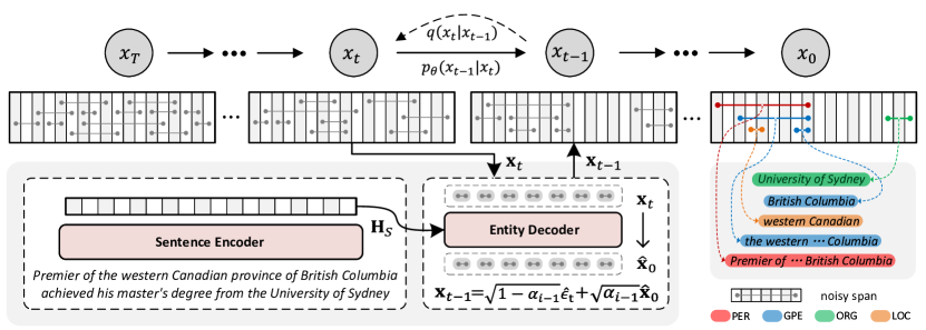
Figure 2: Overview of DiffusionNER. Boundary denoising diffusion process for NER with a denoising network.

4.1 Boundary Denoising Diffusion Model

Given a sentence $S$ with length $M$, the named entity recognition task is to extract the entities $E=\{(l_{i},r_{i},t_{i})\}_{i=0}^{N}$ contained in the sentence, where $N$ is the number of entities and $l_{i},r_{i},t_{i}$ denote the left and right boundary indices and type of the $i$-th entity. We formulate NER as a boundary denoising diffusion process, as shown in Figure 2. We regard entity boundaries as data samples, then the boundary forward diffusion is to add Gaussian noise to the entity boundaries while the reverse diffusion process is to progressively recover the original entity boundaries from the noisy spans.

Boundary Forward Diffusion

Boundary forward diffusion is the process of adding noise to the entity boundary in a stepwise manner. In order to align the number of entities in different instances, we first expand the entity set to a fixed number $K$ ($>N$). There are two ways to expand the entities, repetition strategy and random strategy, which add $K-N$ entities by duplicating entities or sampling random spans from a Gaussian distribution. For convenience, we use $\mathbf{B}\in\mathbb{R}^{K\times 2}$ to denote the boundaries of the $K$ expanded entities, with all of them normalized by the sentence length $M$ and scaled to $(-\lambda,\lambda)$ interval.

Formally, given the entity boundaries as data samples $\mathbf{x}_{0}=\mathbf{B}$, we can obtain the noisy spans at timestep $t$ using the forward diffusion process. According to  Equation 3, we have:

$$\mathbf{x}_{t} =\sqrt{\bar{\alpha}_{t}}\mathbf{x}_{0}+\sqrt{1-\bar{\alpha}_{t}}\epsilon$$ (4)

where $\epsilon\sim\mathcal{N}(\textbf{0},\mathbf{I})$ is the noise sampled from the standard Gaussian. At each timestep, the noisy spans have the same shape as $\mathbf{x}_{0}$, i.e., $\mathbf{x}_{1},\mathbf{x}_{2},\ldots,\mathbf{x}_{T}\in\mathbb{R}^{K\times 2}$.

Boundary Reverse Diffusion

Starting from the noisy spans $\mathbf{x}_{T}$ sampled from the Gaussian distribution, boundary reverse diffusion adopts a non-Markovian denoising practice used in DDIM (Song et al., 2021) to recover entities boundaries. Assuming $\tau$ is an arithmetic subsequence of the complete timestep sequence $[1,\ldots,T]$ of length $\gamma$ with $\tau_{\gamma}=T$. Then we refine the noisy spans $\mathbf{x}_{\tau_{i}}$ to $\mathbf{x}_{\tau_{i-1}}$ as follows:

$$\mathbf{\hat{x}}_{0} =f_{\theta}(\mathbf{x}_{\tau_{i}},S,\tau_{i})$$ (5)

$$\mathbf{\hat{\epsilon}}_{\tau_{i}} =\frac{\mathbf{x}_{\tau_{i}}-\sqrt{\alpha_{\tau_{i}}}\mathbf{\hat{x}}_{0}}{\sqrt{1-\alpha_{\tau_{i}}}}$$ (6)

$$\mathbf{x}_{\tau_{i-1}}= \sqrt{\alpha_{\tau_{i-1}}}\mathbf{\hat{x}}_{0}+\sqrt{1-\alpha_{\tau_{i-1}}}\mathbf{\hat{\epsilon}}_{\tau_{i}}$$ (7)

where $\mathbf{\hat{x}}_{0}$ and $\mathbf{\hat{\epsilon}}_{\tau_{i}}$ are the predicted entity boundary and noise at timestep $\tau_{i}$. $f_{\theta}(\mathbf{x}_{t},S,t)$ is a learnable denoising network and we will cover the network architecture in the next section (§ 4.2). After $\gamma$ iterations of DDIM, the noisy spans are progressively refined to the entity boundaries.

4.2 Network Architecture

Denoising network $f_{\theta}(\mathbf{x}_{t},S,t)$ accepts the noisy spans $\mathbf{x}_{t}$ and the sentence $S$ as inputs and predicts the corresponding entity boundaries $\mathbf{\hat{x}}_{0}$. As shown in Figure 2, we parameterize the denoising network with a sentence encoder and an entity decoder.

Sentence Encoder

consists of a BERT (Devlin et al., 2019) plus a stacked bi-directional LSTM. The whole span encoder takes the sentence ${S}$ as input and outputs the sentence encoding $\mathbf{H}_{S}\in\mathbb{R}^{M\times h}$. The sentence encoding $\mathbf{H}_{S}$ will be calculated only once and reused across all timesteps to save computations.

Entity Decoder

uses the sentence encoding $\mathbf{H}_{S}$ to first compute the representations of $K$ noisy spans $\mathbf{x}_{t}$ and then predicts the corresponding entity boundaries. Specifically, we discretize the noisy spans into word indexes by rescaling, multiplying and rounding, then perform mean pooling over the inner-span tokens. The extracted span representations can be denoted as $\mathbf{H}_{{X}}\in\mathbb{R}^{K\times h}$. To further encode the spans, we design a span encoder that consists of a self-attention and a cross-attention layer. The former enhances the interaction between spans with key, query, and value as $\mathbf{H}_{{X}}$. And the latter fuses the sentence encoding to the span representation with key, value as $\mathbf{H}_{S}$, and query as $\mathbf{H}_{{X}}$. We further add the sinusoidal embedding $\mathbf{E}_{t}$ (Vaswani et al., 2017) of timestep $t$ to the span representations. Thus the new representations $\bar{\mathbf{H}}_{{X}}$ of the noisy spans can be computed:

$$\bar{\mathbf{H}}_{{X}} =\operatorname{SpanEncoder}(\mathbf{H}_{S},\mathbf{H}_{{X}})+\mathbf{E}_{t},$$

Then we use two boundary pointers to predict the entity boundaries. For boundary $\delta\in\{l,r\}$, we compute the fusion representation $\mathbf{H}^{\delta}_{SX}\in\mathbb{R}^{K\times M\times h}$ of the noisy spans and the words, and then the probability of the word as the left or right boundaries $\mathbf{P}^{\delta}\in\mathbb{R}^{K\times M}$ can be computed as:

$$\mathbf{H}^{\delta}_{SX} =\mathbf{H}_{S}\mathbf{W}^{\delta}_{S}+\bar{\mathbf{H}}_{X}\mathbf{W}^{\delta}_{X}$$

$$\mathbf{P}^{\delta} =\operatorname{sigmoid}(\operatorname{MLP}(\mathbf{H}^{\delta}_{SX}))$$

where $\mathbf{W}^{\delta}_{S},\mathbf{W}^{\delta}_{X}\in\mathbb{R}^{h\times h}$ are two learnable matrixes and MLP is a two-layer perceptron. Based on the boundary probabilities, we can predict the boundary indices of the $K$ noisy spans. If the current step is not the last denoising step, we compute $\mathbf{\hat{x}}_{0}$ by normalizing the indices with sentence length $M$ and scaling to $(-\lambda,\lambda)$ intervals. Then we conduct the next iteration of the reverse diffusion process according to Equations 5 to 7.

1 repeat

2       Sample a sentence $S$ with entities $E$ from $\mathcal{D}$

3       Expand $E$ and get entity boundaries B

4       $\mathbf{x}_{0}=\textbf{B}\in\mathbb{R}^{K\times 2}$

5       $t\sim$ Uniform $(\{1,\ldots,T\})$

6       $\epsilon\sim\mathcal{N}(\mathbf{0},\mathbf{I})$

7       $\mathbf{x}_{t}=\sqrt{\bar{\alpha}_{t}}\mathbf{x}_{0}+\sqrt{1-\bar{\alpha}_{t}}\epsilon$

8       Compute $\mathbf{P}^{l}$, $\mathbf{P}^{r}$ and $\mathbf{P}^{c}$ by running $f_{\theta}(\mathbf{x}_{t},S,t)$

9       Take gradient descent step by optimize $-\sum_{i=1}^{K}\left(\log\mathbf{P}_{i}^{c}(\pi^{c}(i))+\sum_{\delta\in{l,r}}\log\mathbf{P}_{i}^{\delta}(\pi^{\delta}(i))\right)$

10until converged;

Algorithm 1 Training

It is worth noting that we should not only locate entities but also classify them in named entity recognition. Therefore, we use an entity classifier to classify the noisy spans. The classification probability $\mathbf{P}^{c}\in\mathbb{R}^{K\times\mathcal{C}}$ is calculated as follows:

$$\mathbf{P}^{c}=\operatorname{Classifier}(\bar{\mathbf{H}}_{X})$$

where $\mathcal{C}$ is the number of entity types and Classifier is a two-layer perceptron with a softmax layer.

1 $\mathbf{x}_{T}\sim\mathcal{N}(\mathbf{0},\mathbf{I})\in\mathbb{R}^{K_{eval}\times 2}$

2 $\tau$ is an arithmetic sequence of length $\gamma$ with $\tau_{\gamma}=T$

3 for $i=\gamma,\ldots,1$ do

4       Compute $\hat{\mathbf{x}}_{0}$, $\mathbf{P}^{l}$, $\mathbf{P}^{r}$ and $\mathbf{P}^{c}$ via $f_{\theta}(\mathbf{x}_{t},S,t)$

5       $\mathbf{x}_{\tau_{i-1}}=\sqrt{\alpha_{\tau_{i-1}}}\mathbf{\hat{x}}_{0}+\sqrt{1-\alpha_{\tau_{i-1}}}\cdot\frac{\mathbf{x}_{\tau_{i}}-\sqrt{\alpha_{\tau_{i}}}\mathbf{\hat{x}}_{0}}{\sqrt{1-\alpha_{\tau_{i}}}}$

6 end for

7Decode entities ${(l_{i},r_{i},c_{i})}^{K_{eval}}_{i=0}$, where $\delta_{i}=\operatorname{argmax}\mathbf{P}_{i}^{\delta},\delta\in\{l,r,c\}$

8 Perform post-processing on ${(l_{i},r_{i},c_{i})}^{K_{eval}}_{i=0}$

return final entities

Algorithm 2 Inference

Training Objective

With $K$ entities predicted from the noisy spans and $N$ ground-truth entities, we first use the Hungarian algorithm (Kuhn, 1955) to solve the optimal matching $\hat{\pi}$ between the two sets as in Carion et al. (2020). $\hat{\pi}(i)$ denotes the ground-truth entity corresponding to the $i$-th noisy span. Then, we train the boundary reverse process by maximizing the likelihood of the prediction:

$$\mathcal{L}=-\sum_{i=1}^{K}\sum_{\delta\in\{l,r,c\}}\log\mathbf{P}_{i}^{\delta}\left(\hat{\pi}^{\delta}(i)\right)$$

where $\hat{\pi}^{l}(i)$, $\hat{\pi}^{r}(i)$ and $\hat{\pi}^{c}(i)$ denote the left and right boundary indexes and type of the $\hat{\pi}(i)$ entity. Overall, Algorithm 1 displays the whole training procedure of our model for an explanation.

Model	ACE04			ACE05			GENIA			Agerage F1-score
	Pr.	Rec.	F1	Pr.	Rec.	F1	Pr.	Rec.	F1
Tagging-based
Straková et al. (2019)	-	-	81.48	-	-	80.82	-	-	77.80	80.03
Ju et al. (2018)	-	-	-	74.20	70.30	72.20	78.50	71.30	74.70	-
Wang et al. (2020)	86.08	86.48	86.28	83.95	85.39	84.66	79.45	78.94	79.19	83.57
Generation-based
Straková et al. (2019)	-	-	84.40	-	-	84.33	-	-	78.31	82.35
Yan et al. (2021b)	87.27	86.41	86.84	83.16	86.38	84.74	78.87	79.60	79.23	83.60
Tan et al. (2021)	88.46	86.10	87.26	87.48	86.63	87.05	82.31	78.66	80.44	84.91
Lu et al. (2022)	-	-	86.89	-	-	85.78	-	-	-	-
Span-based
Yu et al. (2020)	87.30	86.00	86.70	85.20	85.60	85.40	81.80	79.30	80.50	84.20
Li et al. (2020)	85.05	86.32	85.98	87.16	86.59	86.88	81.14	76.82	78.92	83.92
Shen et al. (2021)	87.44	87.38	87.41	86.09	87.27	86.67	80.19	80.89	80.54	84.87
Wan et al. (2022)	86.70	85.93	86.31	84.37	85.87	85.11	77.92	80.74	79.30	83.57
Lou et al. (2022)	87.39	88.40	87.90	85.97	87.87	86.91	-	-	-	-
Zhu and Li (2022)	88.43	87.53	87.98	86.25	88.07	87.15	-	-	-	-
Yuan et al. (2022b)	87.13	87.68	87.40	86.70	86.94	86.82	80.42	82.06	81.23	85.14
Li et al. (2022a)	87.33	87.71	87.52	85.03	88.62	86.79	83.10	79.76	81.39	85.23
DiffusionNER	88.11	88.66	88.39	86.15	87.72	86.93	82.10	80.97	81.53	85.62

Table 1: Results on nested NER datasets.

4.3 Inference

During inference, DiffusionNER first samples $K_{eval}$ noisy spans from a Gaussian distribution, then performs iterative denoising with the learned boundary reverse diffusion process based on the denoising timestep sequence $\tau$. Then with the predicted probabilities on the boundaries and type, we can decode $K_{eval}$ candidate entities ${(l_{i},r_{i},c_{i})}^{K_{eval}}_{i=0}$, where $\delta_{i}=\operatorname{argmax}\mathbf{P}_{i}^{\delta},\delta\in\{l,r,c\}$. After that, we employ two simple post-processing operations on these candidates: de-duplication and filtering. For spans with identical boundaries, we keep the one with the maximum type probability. For spans with the sum of prediction probabilities less than the threshold $\varphi$, we discard them. The inference procedure is shown in Algorithm 2.

5 Experimental Settings

5.1 Datasets

For nested NER, we choose three widely used datasets for evaluation: ACE04 (Doddington et al., 2004), ACE05 (Walker et al., 2006), and GENIA (Ohta et al., 2002). ACE04 and ACE05 belong to the news domain and GENIA is in the biological domain. For flat NER, we use three common datasets to validate: CoNLL03 (Tjong Kim Sang and De Meulder, 2003), OntoNotes (Pradhan et al., 2013), and MSRA (Levow, 2006). More details about datasets can be found in Appendix B.

5.2 Baselines

We choose a variety of recent advanced methods as our baseline, which include: 1) Tagging-based methods (Straková et al., 2019; Ju et al., 2018; Wang et al., 2020); 2) Span-based methods (Yu et al., 2020; Li et al., 2020; Wan et al., 2022; Lou et al., 2022; Zhu and Li, 2022; Yuan et al., 2022b); 3) Generation-based methods (Tan et al., 2021; Yan et al., 2021b; Lu et al., 2022). More details about baselines can be found in Appendix D.

5.3 Implementation Details

For a fair comparison, we use bert-large (Devlin et al., 2019) on ACE04, ACE05, CoNLL03 and OntoNotes, biobert-large (Chiu et al., 2016) on GENIA and chinese-bert-wwm (Cui et al., 2020) on MSRA. We adopt the Adam (Kingma and Ba, 2015) as the default optimizer with a linear warmup and linear decay learning rate schedule. The peak learning rate is set as $2e-5$ and the batch size is 8. For diffusion model, the number of noisy spans $K$ ($K_{eval}$) is set as 60, the timestep $T$ is 1000, and the sampling timestep $\gamma$ is 5 with a filtering threshold $\varphi=2.5$. The scale factor $\lambda$ for noisy spans is 1.0. Please see Appendix C for more details.

6 Results and Analysis

6.1 Performance

Table 1 illustrates the performance of DiffusionNER as well as baselines on the nested NER datasets. Our results in Table 1 demonstrate that DiffusionNER is a competitive NER method, achieving comparable or superior performance compared to state-of-the-art models on the nested NER. Specifically, on ACE04 and GENIA datasets, DiffusionNER achieves F1 scores of 88.39% and 81.53% respectively, with an improvement of +0.77% and +0.41%. And on ACE05, our method achieves comparable results. Meanwhile, DiffusionNER also shows excellent performance on flat NER, just as shown in Table 2. We find that DiffusionNER outperforms the baselines on OntoNotes with +0.16% improvement and achieves a comparable F1-score on both the English CoNLL03 and the Chinese MSRA. These improvements demonstrate that our DiffusionNER can locate entities more accurately due to the benefits of progressive boundary refinement, and thus obtain better performance. The results also validate that our DiffusionNER can recover entity boundaries from noisy spans via boundary denoising diffusion.

Model	CoNLL03
	Pr.	Rec.	F1
Lu et al. (2022)	-	-	92.99
Shen et al. (2021)	92.13	93.73	92.94
Li et al. (2020)†	92.33	94.61	93.04
Yan et al. (2021b)	92.56	93.56	93.05
Li et al. (2022a)†	92.71	93.44	93.07
DiffusionNER	92.99	92.56	92.78
Model	OntoNotes
	Pr.	Rec.	F1
Yan et al. (2019)	-	-	89.78
Yan et al. (2021b)	89.62	90.92	90.27
Li et al. (2020)†	90.14	89.95	90.02
Li et al. (2022a)†	90.03	90.97	90.50
DiffusionNER	90.31	91.02	90.66
Model	MSRA
	Pr.	Rec.	F1
Yan et al. (2019)	-	-	92.74
Shen et al. (2021)	92.20	90.72	91.46
Li et al. (2020)†	91.98	93.29	92.63
Li et al. (2022a)†	94.88	95.06	94.97
DiffusionNER	95.71	94.11	94.91

Table 2: Results on flat NER datasets. $\dagger$ means that we reproduce the results under the same setting.

6.2 Analysis

Inference Efficiency

To further validate whether our DiffusionNER requires more inference computations, we also conduct experiments to compare the inference efficiency between DiffusionNER and other generation-based models (Lu et al., 2022; Yan et al., 2021a). Just as shown in Table 3, we find that DiffusionNER could achieve better performance while maintaining a faster inference speed with minimal parameter scale. Even with a denoising timestep of $\gamma=10$, DiffusionNER is 18$\times$ and 3$\times$ faster than them. This is because DiffusionNER generates all entities in parallel within several denoising timesteps, which avoids generating the linearized entity sequence in an autoregressive manner. In addition, DiffusionNER shares sentence encoder across timesteps, which further accelerates inference speed.

Model	# P	F1	Sents/s	SpeedUp
Lu et al. (2022)	849M	86.89	1.98	1.00$\times$
Yan et al. (2021a)	408M	86.84	13.75	6.94$\times$
DiffusionNER[τ=1]	381M	88.40	82.44	41.64$\times$
DiffusionNER[τ=5]	381M	88.53	57.08	28.83$\times$
DiffusionNER[τ=10]	381M	88.57	37.10	18.74$\times$

Table 3: Comparison with generation-based methods in terms of parameters, performance, and inference speed. # P means the number of parameters. All experiments are conducted on a single GeForce RTX 3090 with the same setting. The results are reported on ACE04.

Denoising Timesteps

We also conduct experiments to analyze the effect of different denoising timesteps on model performance and inference speed of DiffusionNER under various numbers of noisy spans. Just as shown in Figure 3, we find that, with an increase of denoising steps, the model obtains incremental performance improvement while sacrificing inference speed. Considering the trade-off between performance and efficiency, we set $\gamma=5$ as the default setting. In addition, when the noisy spans are smaller, the improvement brought by increasing the denoising timesteps is more obvious. This study indicates that our DiffusionNER can effectively counterbalance the negative impact of undersampling noise spans on performance by utilizing additional timesteps.

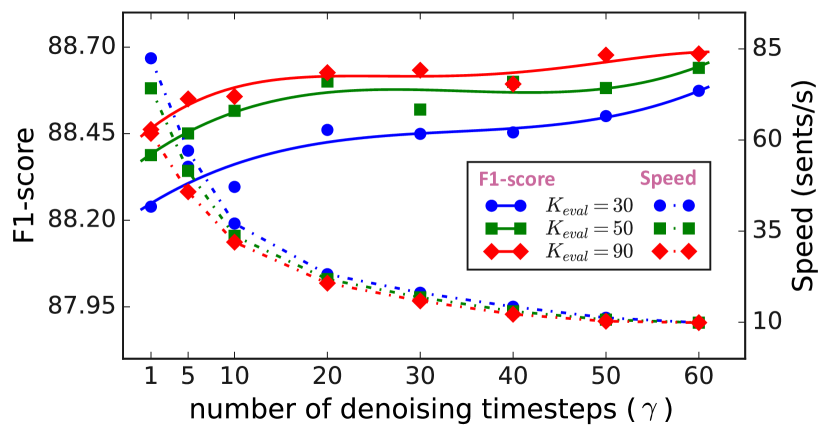
Figure 3: Analysis of denoising timestep $\gamma$ on ACE04.

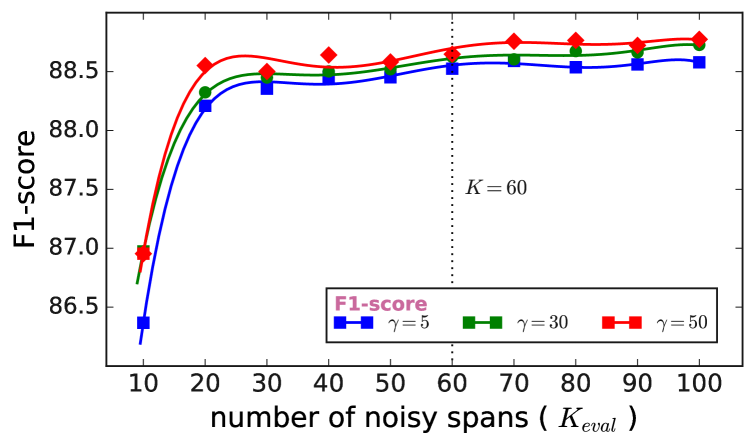
Figure 4: Analysis of #sampled noisy spans on ACE04.

Sampling Number

As a generative latent model, DiffusionNER can decouple training and evaluation, and dynamically sample noisy spans during evaluation. To manifest this advantage, we train DiffusionNER on ACE04 with $K=60$ noisy spans and evaluate it with different sampling numbers $K_{eval}$. The results are shown in Figure 4. Overall, the model performance becomes better as the sampling number of noisy spans increases. Specifically, we find that DiffusionNER performs worse when $K_{eval}<30$. We guess this is because fewer noisy spans may not cover all potential entities. When sampling number $K_{eval}>60$, we find it could also slightly improve model performance. Overall, the dynamic sampling of noisy spans in DiffusionNER has the following advantages: 1) we can improve model performance by controlling it to sample more noisy spans; 2) dynamic sampling strategy also allows the model to predict an arbitrary number of entities in any real-world application, avoiding the limitations of the sampling number at the training stage.

6.3 Ablation Study

Network Architecture

As shown in Table 4, we conduct experiments to investigate the network architecture of the boundary reverse diffusion process. We found that DiffusionNER performs better with a stronger pre-trained language model (PLM), as evidenced by an improvement of +0.53% on ACE04 and +0.11% on CoNLL03 when using roberta-large. Additionally, for the span encoder, we find that directly removing self-attention between noisy spans or cross-attention of spans to the sentence can significantly impair performance. When both are ablated, model performance decreases by 1.37% and 1.15% on ACE04 and CoNLL03. These results indicate that the interaction between the spans or noisy spans and the sentence is necessary.

	Setting	ACE04	CoNLL03
PLM	RoBERTa-Large	88.99	92.89
	BERT-Large	88.39	92.78
	BERT-Base	86.93	92.02
Module	Default	88.39	92.78
	w/o self-attention	87.94	92.25
	w/o cross-attention	87.22	91.40
	w/o span encoder	87.09	91.63

Table 4: Ablation study of network architecture.

Variance Scheduler

The variance scheduler plays a crucial role in controlling the intensity of the added noise at each timestep during boundary forward diffusion process. Therefore, we analyze the performance of DiffusionNER on different variance schedulers with different noise timesteps $T$. The results on ACE04 and CoNLL03 are shown in Table 5. We find that the cosine scheduler generally yields superior results on the ACE04, while the linear scheduler proves to be more effective on CoNLL03. In addition, the performance of DiffusionNER varies with the choice of noise timestep, with the best performance achieved at $T=1000$ for ACE04 and $T=1500$ for CoNLL03.

Scheduler	Timesteps ($T$)	ACE04	CoNLL03
cosine	${T=1000}$	88.39	91.56
	${T=1500}$	87.49	92.04
	${T=2000}$	88.33	91.79
linear	${T=1000}$	88.38	92.78
	${T=1500}$	87.83	92.87
	${T=2000}$	88.17	92.56

Table 5: Ablation study of variance scheduler.

Strategy	# Noisy Spans	ACE04	CoNLL03
Repetition	${K=\ \ 60}$	88.15	92.66
	${K=120}$	88.49	92.54
	${K=150}$	88.19	92.71
Random	${K=\ \ 60}$	88.46	92.78
	${K=120}$	88.53	92.79
	${K=150}$	88.11	92.60

Table 6: Ablation study of expansion strategy.

Expansion Stratagy

The expansion stratagy of the entity set can make the number of $K$ noisy spans consistent across instances during training. We conduct experiments to analyze the performance of DiffusionNER for different expansion strategies with various numbers of noisy spans. The experimental results are shown in Table 6. Generally, we find that the random strategy could achieve similar or better performance than the repetitive strategy. In addition, Table 6 shows that DiffusionNER is insensitive to the number of noisy spans during training. Considering that using more noisy spans brings more computation and memory usage, we set $K=60$ as the default setting.

7 Conclusion

In this paper, we present DiffusionNER, a novel generative approach for NER that converts the task into a boundary denoising diffusion process. Our evaluations on six nested and flat NER datasets show that DiffusionNER achieves comparable or better performance compared to previous state-of-the-art models. Additionally, our additional analyses reveal the advantages of DiffusionNER in terms of inference speed, progressive boundary refinement, and dynamic entity sampling. Overall, this study is a pioneering effort of diffusion models for extractive tasks on discrete text sequences, and we hope it may serve as a catalyst for more research about the potential of diffusion models in natural language understanding tasks.

Limitations

We discuss here the limitations of the proposed DiffusionNER. First, as a latent generative model, DiffusionNER relies on sampling from a Gaussian distribution to produce noisy spans, which leads to a random characteristic of entity generation. Second, DiffusionNER converges slowly due to the denoising training and matching-based loss over a large noise timestep. Finally, since discontinuous named entities often contain multiple fragments, DiffusionNER currently lacks the ability to generate such entities. We can design a simple classifier on top of DiffusionNER, which is used to combine entity fragments and thus solve the problem of discontinuous NER.

Appendix A Optimal Matching $\hat{\pi}$

Given a fixed-size set of $K$ noisy spans, DiffusionNER infers $K$ predictions, where $K$ is larger than the number of $N$ entities in a sentence. One of the main difficulties of training is to assign the ground truth to the prediction. Thus we first produce an optimal bipartite matching between predicted and ground truth entities and then optimize the likelihood-based loss.

Assuming that $\hat{Y}=\{\hat{Y}_{i}\}^{K}_{i=1}$ are the set of $K$ predictions, where $\hat{Y}_{i}=\left(\mathbf{P}_{i}^{l},\mathbf{P}_{i}^{r},\mathbf{P}_{i}^{c}\right)$. We denote the ground truth set of $N$ entities as $Y=\left\{\left(l_{i},r_{i},c_{i}\right)\right\}_{i=1}^{N}$, where $l_{i},r_{i},c_{i}$ are the boundary indices and type for the $i$-th entity. Since $K$ is larger than the number of $N$ entities, we pad $Y$ with $\varnothing$ (no entity). To find a bipartite matching between these two sets we search for a permutation of $K$ elements $\pi\in\mathfrak{S}(K)$ with the lowest cost:

$$\hat{\pi}=\underset{\pi\in\mathfrak{S}(K)}{\arg\min}\sum_{i}^{K}\mathcal{L}_{\operatorname{match}}\left(\hat{Y}_{i},{Y}_{\pi(i)}\right)$$

where $\mathcal{L}_{\operatorname{match}}\left(\hat{Y}_{i},{Y}_{\pi(i)}\right)$ is a pair-wise matching cost between the prediction $\hat{Y}_{i}$ and ground truth ${Y}_{\pi(i)}$ with index $\pi(i)$. We define it as $-\mathds{1}({Y}_{\pi(i)}\neq\varnothing)\sum_{\sigma\in\{l,r,c\}}\mathbf{P}_{i}^{\sigma}\left(Y^{\sigma}_{\pi(i)}\right)$, where $\mathds{1}(\cdot)$ denotes an indicator function. Finally, the optimal assignment $\hat{\pi}$ can be computed with the Hungarian algorithm.

	ACE04			ACE05			GENIA
	Train	Dev	Test	Train	Dev	Test	Train	Test
number of sentences	6200	745	812	7194	969	1047	16692	1854
- with nested entities	2712	294	388	2691	338	320	3522	446
number of entities	22204	2514	3035	24441	3200	2993	50509	5506
- nested entities	10149	1092	1417	9389	1112	1118	9064	1199
- nesting ratio (%)	45.71	46.69	45.61	38.41	34.75	37.35	17.95	21.78
average sentence length	22.50	23.02	23.05	19.21	18.93	17.2	25.35	25.99
maximum number of entities	28	22	20	27	23	17	25	14
average number of entities	3.58	3.37	3.73	3.39	3.30	2.86	3.03	2.97

	CoNLL03			OntoNotes			Chinese MSRA
	Train	Dev	Test	Train	Dev	Test	Train	Dev	Test
number of sentences	14041	3250	3453	49706	13900	10348	41728	4636	4365
number of entities	23499	5942	5648	128738	20354	12586	70446	4257	6181
average sentence length	14.50	15.80	13.45	24.94	20.11	19.74	46.87	46.17	39.54
maximum number of entities	20	20	31	32	71	21	125	18	461
average number of entities	1.67	1.83	1.64	2.59	1.46	1.22	1.69	0.92	1.42

Table 7: Statistics of the nested and flat datasets used in our experiments.

Appendix B Datasets

We conduct experiments on six widely used NER datasets, including three nested and three flat datasets. Table 7 reports detailed statistics about the datasets.

ACE04 and ACE05

(Doddington et al., 2004; Walker et al., 2006) are two nested NER datasets and contain 7 entity categories, including PER, ORG, LOC, GPE, WEA, FAC and VEH categories. We follow the same setup as previous works Katiyar and Cardie (2018); Lin et al. (2019).

GENIA

(Ohta et al., 2002) is a biology nested NER dataset and contains 5 entity types, including DNA, RNA, protein, cell line and cell type categories. Follow Huang et al. (2022); Shen et al. (2021), we train the model on the concatenation of the train and dev sets.

CoNLL03

(Tjong Kim Sang and De Meulder, 2003) is a flat dataset with 4 types of named entities: LOC, ORG, PER and MISC. Follow Yu et al. (2020); Yan et al. (2021c); Shen et al. (2021), we train our model on the combination of the train and dev sets.

OntoNotes

(Pradhan et al., 2013) is a flat dataset with 18 types of named entities, including 11 entity types and 7 value types. We use the same train, development, and test splits as Li et al. (2020); Shen et al. (2022).

MSRA

(Levow, 2006) is a Chinese flat dataset with 3 entity types, including ORG, PER, LOC. We keep the same dataset splits and pre-processing with Li et al. (2022a); Shen et al. (2021).

Appendix C Detailed Parameter Settings

Entity boundaries are predicted at the word level, and we use max-pooling to aggregate subwords into word representations. We use the multi-headed attention with 8 heads in the span encoder, and add a feedforward network layer after the self-attention and cross-attention layer. During training, we first fix the parameters of BERT and train the model for $5$ epochs to warm up the parameters of the entity decoder. We tune the learning rate from $\{1e-5,2e-5,3e-5\}$ and the threshold $\varphi$ from range $[2.5,2.7]$ with a step $0.05$, and select the best hyperparameter setting according to the performance of the development set. The detailed parameter settings are shown in Table 8.

Hyperparameter	ACE04	ACE05	GENIA
learning rate	2e-5	3e-5	2e-5
weight decay	0.1	0.1	0.1
lr warmup	0.1	0.1	0.1
batch size	8	8	8
epoch	100	50	50
hidden size $h$	1024	1024	1024
threshold $\varphi$	2.55	2.65	2.50
scale factor $\lambda$	1.0	1.0	2.0

Hyperparameter	CoNLL03	Ontonotes	MSRA
learning rate	2e-5	2e-5	5e-6
weight decay	0.1	0.1	0.1
lr warmup	0.1	0.1	0.1
batch size	8	8	16
epoch	100	50	100
hidden size $h$	1024	1024	768
threshold $\varphi$	2.50	2.55	2.60
scale factor $\lambda$	1.0	2.0	1.0

Table 8: Detailed Hyperparameter Settings

Appendix D Baselines

We use the following models as baselines:

• LinearedCRF (Straková et al., 2019) concatenates the nested entity multiple labels into one multilabel, and uses CRF-based tagger to decode flat or nested entities.

• CascadedCRF (Ju et al., 2018) stacks the flat NER layers and identifies nested entities in an inside-to-outside way.

• Pyramid (Wang et al., 2020) constructs the representations of mentions from the bottom up by stacking flat NER layers in a pyramid, and allows bidirectional interaction between layers by an inverse pyramid.

• Seq2seq (Straková et al., 2019) converts the labels of nested entities into a sequence and then uses a seq2seq model to decode entities.

• BARTNER (Yan et al., 2021b) is also a sequence-to-sequence framework that transforms entity labels into word index sequences and decodes entities in a word-pointer manner.

• Seq2Set (Tan et al., 2021)treats NER as a sequence-to-set task and constructs learnable entity queries to generate entities.

• UIE (Lu et al., 2022) designs a special schema for the conversion of structured information to sequences, and adopts a generative model to generate linearized sequences to unify various information extraction tasks.

• Biaffine (Yu et al., 2020) reformulates NER as a structured prediction task and adopts a dependency parsing approach for NER.

• MRC (Li et al., 2020) reformulates NER as a reading comprehension task and extracts entities to answer the type-specific questions.

• Locate&label (Shen et al., 2021) is a two-stage method that first regresses boundaries to locate entities and then performs entity typing.

• SpanGraph (Wan et al., 2022) utilizes a retrieval-based span-level graph to improve the span representation, which can connect spans and entities in the training data.

• LLCP (Lou et al., 2022) treat NER as latent lexicalized constituency parsing and resort to constituency trees to model nested entities.

• BoundarySmooth (Zhu and Li, 2022), inspired by label smoothing, proposes boundary smoothing for span-based NER methods.

• Triffine (Yuan et al., 2022b) proposes a triaffine mechanism to integrate heterogeneous factors to enhance the span representation, including inside tokens, boundaries, labels, and related spans.

• Word2Word (Li et al., 2022a) treats NER as word-word relation classification and uses multi-granularity 2D convolutions to construct the 2D word-word grid representations.

References

- Amit et al. (2021) Tomer Amit, Eliya Nachmani, Tal Shaharbany, and Lior Wolf. 2021. Segdiff: Image segmentation with diffusion probabilistic models. ArXiv, abs/2112.00390.
- Athiwaratkun et al. (2020) Ben Athiwaratkun, Cicero Nogueira dos Santos, Jason Krone, and Bing Xiang. 2020. Augmented natural language for generative sequence labeling. In Proceedings of the 2020 Conference on Empirical Methods in Natural Language Processing (EMNLP), pages 375–385, Online. Association for Computational Linguistics.
- Austin et al. (2021) Jacob Austin, Daniel D. Johnson, Jonathan Ho, Daniel Tarlow, and Rianne van den Berg. 2021. Structured denoising diffusion models in discrete state-spaces. In Advances in Neural Information Processing Systems, volume 34, pages 17981–17993. Curran Associates, Inc.
- Baranchuk et al. (2022) Dmitry Baranchuk, Andrey Voynov, Ivan Rubachev, Valentin Khrulkov, and Artem Babenko. 2022. Label-efficient semantic segmentation with diffusion models. In International Conference on Learning Representations.
- Carion et al. (2020) Nicolas Carion, Francisco Massa, Gabriel Synnaeve, Nicolas Usunier, Alexander Kirillov, and Sergey Zagoruyko. 2020. End-to-end object detection with transformers. In Computer Vision – ECCV 2020, pages 213–229, Cham. Springer International Publishing.
- Chen et al. (2022) Shoufa Chen, Peize Sun, Yibing Song, and Ping Luo. 2022. Diffusiondet: Diffusion model for object detection. arXiv preprint arXiv:2211.09788.
- Chiu et al. (2016) Billy Chiu, Gamal Crichton, Anna Korhonen, and Sampo Pyysalo. 2016. How to train good word embeddings for biomedical NLP. In Proceedings of the 15th Workshop on Biomedical Natural Language Processing, pages 166–174, Berlin, Germany. Association for Computational Linguistics.
- Chiu and Nichols (2016) Jason P.C. Chiu and Eric Nichols. 2016. Named Entity Recognition with Bidirectional LSTM-CNNs. Transactions of the Association for Computational Linguistics, 4:357–370.
- Cui et al. (2020) Yiming Cui, Wanxiang Che, Ting Liu, Bing Qin, Shijin Wang, and Guoping Hu. 2020. Revisiting pre-trained models for Chinese natural language processing. In Findings of the Association for Computational Linguistics: EMNLP 2020, pages 657–668, Online. Association for Computational Linguistics.
- De Cao et al. (2021) Nicola De Cao, Gautier Izacard, Sebastian Riedel, and Fabio Petroni. 2021. Autoregressive entity retrieval. In 9th International Conference on Learning Representations, ICLR 2021, Virtual Event, Austria, May 3-7, 2021. OpenReview.net.
- Devlin et al. (2019) Jacob Devlin, Ming-Wei Chang, Kenton Lee, and Kristina Toutanova. 2019. BERT: Pre-training of deep bidirectional transformers for language understanding. In Proceedings of the 2019 Conference of the North American Chapter of the Association for Computational Linguistics: Human Language Technologies, Volume 1 (Long and Short Papers), pages 4171–4186, Minneapolis, Minnesota. Association for Computational Linguistics.
- Doddington et al. (2004) George Doddington, Alexis Mitchell, Mark Przybocki, Lance Ramshaw, Stephanie Strassel, and Ralph Weischedel. 2004. The automatic content extraction (ACE) program – tasks, data, and evaluation. In Proceedings of the Fourth International Conference on Language Resources and Evaluation (LREC’04), Lisbon, Portugal. European Language Resources Association (ELRA).
- Eberts and Ulges (2020) Markus Eberts and Adrian Ulges. 2020. Span-based joint entity and relation extraction with transformer pre-training. In Proceedings of the 24th European Conference on Artificial Intelligence, Santiago de Compostela, Spain.
- Gong et al. (2022) Shansan Gong, Mukai Li, Jiangtao Feng, Zhiyong Wu, and Lingpeng Kong. 2022. Diffuseq: Sequence to sequence text generation with diffusion models. arXiv preprint arXiv:2210.08933.
- He et al. (2022) Zhengfu He, Tianxiang Sun, Kuanning Wang, Xuanjing Huang, and Xipeng Qiu. 2022. Diffusionbert: Improving generative masked language models with diffusion models. arXiv preprint arXiv:2211.15029.
- Ho et al. (2020) Jonathan Ho, Ajay Jain, and Pieter Abbeel. 2020. Denoising diffusion probabilistic models. In Advances in Neural Information Processing Systems, volume 33, pages 6840–6851. Curran Associates, Inc.
- Hoogeboom et al. (2022) Emiel Hoogeboom, Alexey A. Gritsenko, Jasmijn Bastings, Ben Poole, Rianne van den Berg, and Tim Salimans. 2022. Autoregressive diffusion models. In International Conference on Learning Representations.
- Huang et al. (2022) Xin Huang, Ashish Khetan, Rene Bidart, and Zohar Karnin. 2022. Pyramid-BERT: Reducing complexity via successive core-set based token selection. In Proceedings of the 60th Annual Meeting of the Association for Computational Linguistics (Volume 1: Long Papers), pages 8798–8817, Dublin, Ireland. Association for Computational Linguistics.
- Ju et al. (2018) Meizhi Ju, Makoto Miwa, and Sophia Ananiadou. 2018. A neural layered model for nested named entity recognition. In Proceedings of the 2018 Conference of the North American Chapter of the Association for Computational Linguistics: Human Language Technologies, Volume 1 (Long Papers), pages 1446–1459, New Orleans, Louisiana. Association for Computational Linguistics.
- Katiyar and Cardie (2018) Arzoo Katiyar and Claire Cardie. 2018. Nested named entity recognition revisited. In Proceedings of the 2018 Conference of the North American Chapter of the Association for Computational Linguistics: Human Language Technologies, Volume 1 (Long Papers), pages 861–871, New Orleans, Louisiana. Association for Computational Linguistics.
- Kingma and Ba (2015) Diederik P. Kingma and Jimmy Ba. 2015. Adam: A method for stochastic optimization. In 3th International Conference on Learning Representations, ICLR 2021.
- Kong et al. (2021) Zhifeng Kong, Wei Ping, Jiaji Huang, Kexin Zhao, and Bryan Catanzaro. 2021. Diffwave: A versatile diffusion model for audio synthesis. In International Conference on Learning Representations.
- Kuhn (1955) Harold W Kuhn. 1955. The hungarian method for the assignment problem. Naval research logistics quarterly, 2(1-2):83–97.
- Levow (2006) Gina-Anne Levow. 2006. The third international Chinese language processing bakeoff: Word segmentation and named entity recognition. In Proceedings of the Fifth SIGHAN Workshop on Chinese Language Processing, pages 108–117, Sydney, Australia. Association for Computational Linguistics.
- Lewis et al. (2020) Mike Lewis, Yinhan Liu, Naman Goyal, Marjan Ghazvininejad, Abdelrahman Mohamed, Omer Levy, Veselin Stoyanov, and Luke Zettlemoyer. 2020. BART: Denoising sequence-to-sequence pre-training for natural language generation, translation, and comprehension. In Proceedings of the 58th Annual Meeting of the Association for Computational Linguistics, pages 7871–7880, Online. Association for Computational Linguistics.
- Li et al. (2022a) Jingye Li, Hao Fei, Jiang Liu, Shengqiong Wu, Meishan Zhang, Chong Teng, Donghong Ji, and Fei Li. 2022a. Unified named entity recognition as word-word relation classification. In Proceedings of the AAAI Conference on Artificial Intelligence, volume 36, pages 10965–10973.
- Li and Ji (2014) Qi Li and Heng Ji. 2014. Incremental joint extraction of entity mentions and relations. In Proceedings of the 52nd Annual Meeting of the Association for Computational Linguistics (Volume 1: Long Papers), pages 402–412, Baltimore, Maryland. Association for Computational Linguistics.
- Li et al. (2022b) Xiang Lisa Li, John Thickstun, Ishaan Gulrajani, Percy Liang, and Tatsunori Hashimoto. 2022b. Diffusion-lm improves controllable text generation. ArXiv, abs/2205.14217.
- Li et al. (2020) Xiaoya Li, Jingrong Feng, Yuxian Meng, Qinghong Han, Fei Wu, and Jiwei Li. 2020. A unified MRC framework for named entity recognition. In Proceedings of the 58th Annual Meeting of the Association for Computational Linguistics, pages 5849–5859, Online. Association for Computational Linguistics.
- Lin et al. (2019) Hongyu Lin, Yaojie Lu, Xianpei Han, and Le Sun. 2019. Sequence-to-nuggets: Nested entity mention detection via anchor-region networks. In Proceedings of the 57th Annual Meeting of the Association for Computational Linguistics, pages 5182–5192, Florence, Italy. Association for Computational Linguistics.
- Lou et al. (2022) Chao Lou, Songlin Yang, and Kewei Tu. 2022. Nested named entity recognition as latent lexicalized constituency parsing. In Proceedings of the 60th Annual Meeting of the Association for Computational Linguistics (Volume 1: Long Papers), pages 6183–6198, Dublin, Ireland. Association for Computational Linguistics.
- Lu et al. (2022) Yaojie Lu, Qing Liu, Dai Dai, Xinyan Xiao, Hongyu Lin, Xianpei Han, Le Sun, and Hua Wu. 2022. Unified structure generation for universal information extraction. In Proceedings of the 60th Annual Meeting of the Association for Computational Linguistics (Volume 1: Long Papers), pages 5755–5772, Dublin, Ireland. Association for Computational Linguistics.
- McClosky et al. (2011) David McClosky, Mihai Surdeanu, and Christopher Manning. 2011. Event extraction as dependency parsing. In Proceedings of the 49th Annual Meeting of the Association for Computational Linguistics: Human Language Technologies, pages 1626–1635, Portland, Oregon, USA. Association for Computational Linguistics.
- Miwa and Bansal (2016) Makoto Miwa and Mohit Bansal. 2016. End-to-end relation extraction using LSTMs on sequences and tree structures. In Proceedings of the 54th Annual Meeting of the Association for Computational Linguistics (Volume 1: Long Papers), pages 1105–1116, Berlin, Germany. Association for Computational Linguistics.
- Ohta et al. (2002) Tomoko Ohta, Yuka Tateisi, and Jin-Dong Kim. 2002. The genia corpus: An annotated research abstract corpus in molecular biology domain. In Proceedings of the Second International Conference on Human Language Technology Research, page 82–86, San Francisco, USA. Morgan Kaufmann Publishers Inc.
- Paolini et al. (2021) Giovanni Paolini, Ben Athiwaratkun, Jason Krone, Jie Ma, Alessandro Achille, RISHITA ANUBHAI, Cicero Nogueira dos Santos, Bing Xiang, and Stefano Soatto. 2021. Structured prediction as translation between augmented natural languages. In International Conference on Learning Representations.
- Pradhan et al. (2013) Sameer Pradhan, Alessandro Moschitti, Nianwen Xue, Hwee Tou Ng, Anders Björkelund, Olga Uryupina, Yuchen Zhang, and Zhi Zhong. 2013. Towards robust linguistic analysis using OntoNotes. In Proceedings of the Seventeenth Conference on Computational Natural Language Learning, pages 143–152, Sofia, Bulgaria. Association for Computational Linguistics.
- Raffel et al. (2020) Colin Raffel, Noam Shazeer, Adam Roberts, Katherine Lee, Sharan Narang, Michael Matena, Yanqi Zhou, Wei Li, and Peter J. Liu. 2020. Exploring the limits of transfer learning with a unified text-to-text transformer. Journal of Machine Learning Research, 21(140):1–67.
- Ramesh et al. (2022) Aditya Ramesh, Prafulla Dhariwal, Alex Nichol, Casey Chu, and Mark Chen. 2022. Hierarchical text-conditional image generation with clip latents.
- Rombach et al. (2022) Robin Rombach, Andreas Blattmann, Dominik Lorenz, Patrick Esser, and Björn Ommer. 2022. High-resolution image synthesis with latent diffusion models. In 2022 IEEE/CVF Conference on Computer Vision and Pattern Recognition (CVPR), pages 10674–10685.
- Shen et al. (2021) Yongliang Shen, Xinyin Ma, Zeqi Tan, Shuai Zhang, Wen Wang, and Weiming Lu. 2021. Locate and label: A two-stage identifier for nested named entity recognition. In Proceedings of the 59th Annual Meeting of the Association for Computational Linguistics and the 11th International Joint Conference on Natural Language Processing (Volume 1: Long Papers), pages 2782–2794, Online. Association for Computational Linguistics.
- Shen et al. (2022) Yongliang Shen, Xiaobin Wang, Zeqi Tan, Guangwei Xu, Pengjun Xie, Fei Huang, Weiming Lu, and Yueting Zhuang. 2022. Parallel instance query network for named entity recognition. In Proceedings of the 60th Annual Meeting of the Association for Computational Linguistics (Volume 1: Long Papers), pages 947–961, Dublin, Ireland. Association for Computational Linguistics.
- Sohl-Dickstein et al. (2015) Jascha Sohl-Dickstein, Eric Weiss, Niru Maheswaranathan, and Surya Ganguli. 2015. Deep unsupervised learning using nonequilibrium thermodynamics. In Proceedings of the 32nd International Conference on Machine Learning, volume 37 of Proceedings of Machine Learning Research, pages 2256–2265, Lille, France. PMLR.
- Sohrab and Miwa (2018) Mohammad Golam Sohrab and Makoto Miwa. 2018. Deep exhaustive model for nested named entity recognition. In Proceedings of the 2018 Conference on Empirical Methods in Natural Language Processing, pages 2843–2849, Brussels, Belgium. Association for Computational Linguistics.
- Song et al. (2021) Jiaming Song, Chenlin Meng, and Stefano Ermon. 2021. Denoising diffusion implicit models. In International Conference on Learning Representations.
- Straková et al. (2019) Jana Straková, Milan Straka, and Jan Hajic. 2019. Neural architectures for nested NER through linearization. In Proceedings of the 57th Annual Meeting of the Association for Computational Linguistics, pages 5326–5331, Florence, Italy. Association for Computational Linguistics.
- Strudel et al. (2022) Robin Strudel, Corentin Tallec, Florent Altché, Yilun Du, Yaroslav Ganin, Arthur Mensch, Will Grathwohl, Nikolay Savinov, Sander Dieleman, Laurent Sifre, et al. 2022. Self-conditioned embedding diffusion for text generation. arXiv preprint arXiv:2211.04236.
- Tan et al. (2021) Zeqi Tan, Yongliang Shen, Shuai Zhang, Weiming Lu, and Yueting Zhuang. 2021. A sequence-to-set network for nested named entity recognition. In Proceedings of the Thirtieth International Joint Conference on Artificial Intelligence, IJCAI-21, pages 3936–3942. International Joint Conferences on Artificial Intelligence Organization. Main Track.