Bound and Optimal Design of Dallenbach Absorber Under Finite-Bandwidth Multiple-Angle Illumination

Abstract

Dallenbach absorbers are lossy substances attached to a perfect electric conductor sheet. For such a configuration Rozanov derived a sum rule that relates the absorber’s efficacy with its thickness and frequency-band of operation. Rozanov’s derivation is valid only for layer impinged by a normally incident plane wave. Later, this relation was extended for oblique incidence considering both transverse electric and transverse magnetic polarizations. Here, we follow the same approach and present a sum rule that is valid for multiple and possibly a spectrum of oblique incident waves which are arbitrarily weighted. We recast the design of the Dallenbach absorber as an optimization problem, where optimization is performed over its electromagnetic properties. The optimization problem is applicable for practical implementations where finite spectral bandwidth is considered, as well as for theoretical aspects such as determining the tightness of the sum rule over an infinite bandwidth. We provide a numerical example for a practical case where we perform an optimization procedure for a given weight function and finite bandwidth. Additionally, we demonstrate the effect of the weight function on the optimization results.

I Introduction

Wave absorbers have been fascinating researchers throughout the history [1, 2, 3, 4, 5, 6, 7, 8, 9, 10, 11], as they are being used in a variety of electromagnetic applications such as reducing reflections [12, 13, 14, 15], enhanced accuracy of antenna measurements in anechoic chambers [16, 17, 18], decreasing undesired emissions of discrete electric components and printed circuit boards (PCBs) [19, 20, 21] and to capture light in solar cells [22, 23], to name a few. Among the different types of wave absorbers, Dallenbach layer, a lossy substance backed by a perfect electric conductor (PEC) sheet, is widely used due to its compatibility with planar geometries [1]. Rozanov [24] has derived a sum rule relation, a bound, between the absorption efficacy, thickness and the operating frequency band that is valid when the absorber is illuminated by a normal incidence plane wave. Rozanov’s derivation relies on the typical assumptions of passivity, linearity and time-invariance (LTI) and causality, while in addition it is based on the long wavelength (i.e. static) behaviour of the reflection coefficient. Over the past few years, several research groups investigated an approach to bypass Rozanov’s bound which involves revoking the time-invariance assumption and permitting certain time-variations in the absorbing structure [25, 26, 27]. However, practical implementation of the proposed designs remains an open challenge. Recently, it was shown by our group [28] that by replacing the PEC boundary with a transparent impedance sheet (inductive, capacitive, or resistive), it is possible to bypass the limits imposed by Rozanov’s bound. Importantly, this improvement was achieved by revoking the last assumption on the long wavelength behaviour of the reflection coefficient without sacrificing the key assumptions of passivity and LTI. For these configurations, when possible, we have also derived the relevant sum rules.

An extension of Rozanov’s bound for oblique incidence of a single plane wave, for both transverse electric (TE) and transverse magnetic (TM) polarizations was proposed by Volakis’s group [29, 30]. Duality principle dictates that these sum rules apply not only for absorbing systems but also for infinite radiating antenna arrays that are placed above a PEC surface. This insight led several researches to use these bounds as a figure of merit in the design of antenna arrays [31, 32]. Here, we extend the sum rule trade-off for the case of multiple and possibly a continuous spectrum of oblique incidence plane waves. Moreover, we introduce in the sum rule the possibility to include an arbitrary angular weight function $W(\theta)$ (for both TE and TM polarizations) that reflects the designer absorption requirements for each angle of incidence. We verify numerically that the new sum rule is tight when integrating along the entire bandwidth spectrum. To account for practical systems that operate in a specific (i.e. finite) bandwidth, we set a non-convex optimization problem to obtain the optimal design parameters, namely the permittivity $\epsilon$ and electric conductivity $\sigma$ of the Dallenbach absorber. While being restricted to the new relation, the optimal solution maximizes the contribution within the desired bandwidth while simultaneously minimizing it outside. We introduce a numerical example that its aim is to optimize a Dallenbach layer with thickness of $0.4\left[\rm{m}\right]$, operating at the free-space bandwidth $0.1$ to $3$ meters subject to a uniform windowed weight function. Moreover, we consider different weight functions over a finite bandwidth and show that distinct optimization parameters are obtained.

II Mathematical Formulation

Consider a Dallenbach planar layer that is backed by a PEC sheet with electrical permittivity ($\epsilon$), magnetic permeability ($\mu$) and electrical conductivity ($\sigma$) surrounded by vacuum ($\epsilon_{0},\mu_{0}$). The layer extends infinitely in the $x$ and $y$ directions and has a finite thickness $d$ in the $z$ direction. The layer is impinged by a wave field that is composed of an angular spectrum of propagating oblique incidence plane waves with either TE or TM polarizations (see Fig. 1 for illustration). Due to the interaction with the Dallenbach layer, some of the wave field is reflected backwards, while the rest is absorbed within the layer. Note that the PEC boundary enforces that there is no transmitted wave beyond the absorbing layer. By following similar approach as in Rozanov’s derivation [24], Volakis’s group proposed a generalized sum rule that is valid for a single oblique incidence plane-wave at an angle $\theta$ with TE or TM polarization [29],

$$\left|\int_{0}^{\infty}\!\!\ln\left|\rho(\lambda,\theta)\right|\!\,d\lambda\right|\leq 2\pi^{2}\mu_{s}d\begin{cases}\rm{cos}\left(\theta\right),&\!\!\rm{TE}\\ 1/\rm{cos}\left(\theta\right),&\!\!\rm{TM}\end{cases}\triangleq\rm{RB}\left(\theta\right).$$ (1)

Where $\rho$ is the reflection coefficient at the interface between the Dallenbach absorber and its surroundings, $\lambda$ is the free space wavelength and $\mu_{s}$ is the static relative permeability. The relationship described in Eq. (1) illustrates a polarization-dependent trade-off between the absorption performance of the layer, its thickness, its static permeability and the angle of incidence. Here, we present an extension to the relationship in Eq. (1) for a wave field that comprises a spectrum (multiple) of oblique incidence plane waves with arbitrary weights. To enrich the discussion for the real-world applications where systems are typically designed to operate at a specific bandwidth, we truncate the wavelength domain into $[\lambda_{1},\lambda_{2}]$, where $\lambda_{1}$ [$\lambda_{2}$] is the minimal [maximal] free-space wavelength of interest. Since both handsides of Eq. (1) are non-negative for any selection of the layer’s characteristic parameters $\{\epsilon,\sigma,\mu\}$, multiplying it by a normalized non-negative weight function $W(\theta)$ and integrating with respect to the angle of incidence ($\theta$) yields,

$$\int_{\theta_{1}}^{\theta_{2}}W(\theta)\left|\int_{\lambda_{1}}^{\lambda_{2}}\!\!\ln\left|\rho(\lambda,\theta)\right|\!\,d\lambda\right|d\theta\leq$$ (2)

$$\int_{\theta_{1}}^{\theta_{2}}W(\theta)\left|\int_{0}^{\infty}\!\!\ln\left|\rho(\lambda,\theta)\right|\!\,d\lambda\right|d\theta\leq\int_{\theta_{1}}^{\theta_{2}}W(\theta)\rm{RB}\left(\theta\right)d\theta,$$

where $[\theta_{1},\theta_{2}]$ are the minimal and maximal desired angles of incidence, respectively and $\int_{\theta_{1}}^{\theta_{2}}W(\theta)d\theta=1,\hskip 2.84544ptW(\theta)\geq 0\hskip 2.84544pt\forall\hskip 2.84544pt\theta\in[\theta_{1},\theta_{2}]$. The relationship in Eq. (2) describes the appropriate sum rule (bound) for wave fields composed of a spectrum (multiple) of oblique incidence plane waves with arbitrary weights. The right hand side of Eq. (2) bounds from above the left and middle sides for any selection of the properties of the layers (namely $\{\epsilon,\mu,\sigma\}$). This gives rise to an optimization problem for designing a Dallenbach absorber. By employing Eq. (2) as a $W$-weighted $L^{1}$ norm on $\theta$ space, we formulate the following optimization problem to obtain the absorber’s characteristic parameters,

$$\min_{\epsilon,\sigma}\int_{\theta_{1}}^{\theta_{2}}\left|W(\theta)\rm{RB}-W(\theta)\left|\int_{\lambda_{1}}^{\lambda_{2}}\!\!\ln\left|\rho(\lambda,\theta)\right|\!\,d\lambda\right|\right|d\theta$$ (3)

$$\rm{subject\hskip 5.69046ptto}\hskip 28.45274pt\rho(\lambda,\theta)=\frac{Z_{\mbox{\scriptsize in}}(\lambda,\theta)-\eta_{0}(\theta)}{Z_{\mbox{\scriptsize in}}(\lambda,\theta)+\eta_{0}(\theta)}.$$

The impedance $Z_{\mbox{\scriptsize in}}$ refers to the input impedance at the interface between the absorbing layer and its surroundings, while $\eta_{0}$ is the free space (TE and TM) characteristic impedance (see [33, 34, 35]). An alternative (equivalent) way to express (3) as a maximization problem is to normalize the cost function by dividing Eq. (2) by its right-hand side. The resulting value of the expression is between $0$ and $1$, where a score of $1$ indicates the highest achievable value of the cost function, i.e., tightest bound, for any given set of design parameters ($\epsilon,\sigma$). The alternative optimization problem reads,

$$\max_{\epsilon,\sigma}\hskip 5.69046pt\frac{\int_{\theta_{1}}^{\theta_{2}}W(\theta)\left|\int_{\lambda_{1}}^{\lambda_{2}}\ln\left|\rho(\lambda,\theta)\right|\!\,d\lambda\right|d\theta}{\int_{\theta_{1}}^{\theta_{2}}W(\theta)\rm{RB}\left(\theta\right)d\theta}$$ (4)

$$\rm{subject\hskip 5.69046ptto}\hskip 11.38092pt\rho(\lambda,\theta)=\frac{Z_{\mbox{\scriptsize in}}(\lambda,\theta)-\eta_{0}(\theta)}{Z_{\mbox{\scriptsize in}}(\lambda,\theta)+\eta_{0}(\theta)}.$$

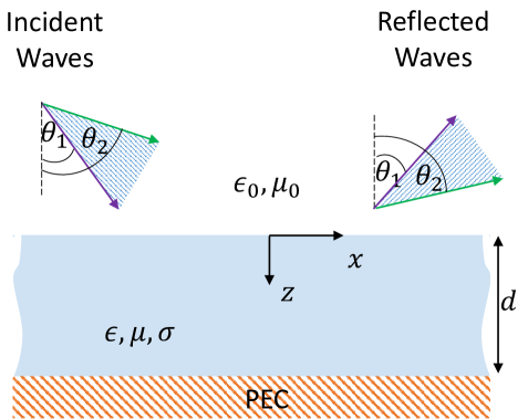
Figure 1: Illustration of the problem. A Dallenbach layer with thickness $d$ is impinged by a wave field that is composed of multiple propagating plane waves within the angular domain $\theta\in\left[\theta_{1},\theta_{2}\right]$. As a result of the interaction with the Dallenbach layer, a portion of the wave field is reflected backwards, while the remaining portion is absorbed inside the layer. The wave field may consist of either one or both of the TE and TM polarizations.

In the following sections we use Eqs. (2)-(4) to explore the tightness of the new sum rule and to design a practical Dallenbach absorber that operates within a finite frequency spectrum and angular spectrum of incidence waves. In addition we explore the influence of the weight function on the optimization results.

III The Tightness of the Sum Rule

Here, we aim to verify the tightness of the sum rule in Eq. (2), for the case of a wave field with an infinite frequency spectrum within the angular domain $[\theta_{1},\theta_{2}]=[0,\pi/3]$. For that purpose we consider a non-magnetic layer ($\mu=\mu_{0},\mu_{s}=1$) with thickness $d=0.4\left[\rm{m}\right]$. The layer is composed of wavelength dependent permittivity $\epsilon\left(\lambda\right)$ and electric conductivity $\sigma(\lambda)$ having a Lorentzian form (note that these parameters satisfy Kramers–Kronig relations - a fundamental requirement for causal materials, [36]),

$$\epsilon\left(\lambda\right) =\epsilon_{0}\left(1+\frac{A}{1+j\frac{\lambda_{\rm{rel}}}{\lambda}-(\frac{\lambda_{\rm{res}}}{\lambda})^{2}}\right)$$ (5)

$$\sigma\left(\lambda\right) =\frac{\sigma_{\rm{s}}}{1+j\frac{2\pi c_{0}\tau_{\sigma}}{\lambda}},$$

where $A$ denotes the strength of the dielectric response, $\lambda_{\rm{res}}[\lambda_{\rm{rel}}]$ is the resonant [relaxation] wavelength, $\sigma_{\rm{s}}$ is the static (long wavelength) electric conductivity, $c_{0}=1/\sqrt{\epsilon_{0}\mu_{0}}$ is the speed of light in vacuum and $\tau_{\sigma}$ is a time constant of the conductor. By combining Ampere’s law with Ohm’s law and Eq. (5), an effective electric permittivity, $\epsilon_{\rm{eff}}(\lambda)$, can be expressed. This effective permittivity takes into account both polarization and conductance effects and is given by $\epsilon_{\rm{eff}}(\lambda)=\epsilon\left(\lambda\right)+\sigma\left(\lambda\right)/(j2\pi c_{0}\lambda^{-1})$.

For the sake of simplicity and concreteness, we set the following parameters: $A=1,\lambda_{\rm{res}}=\lambda_{\rm{rel}}=1\left[\rm{m}\right],\tau_{\sigma}=10^{-12}\left[\rm{sec}\right]$, while the only remaining free-parameter is $\sigma_{\rm{s}}$ that will be scanned over a wide range of values to demonstrate its effect on the tightness of the bound. In addition, we define three weight functions {$W_{1}(\theta),W_{2}(\theta),W_{3}(\theta)$} within the angular domain $\theta\in[\theta_{1},\theta_{2}]$ (see Fig. 2 (a)),

$$W_{1}(\theta)=\frac{3}{\pi},$$ (6)

$$W_{2}(\theta)=4.5496\hskip 2.84544pt\theta^{5}$$

$$W_{3}(\theta)=5.015\hskip 2.84544pte^{-10|\theta-\pi/6|},$$

and zero elsewhere. The three weight functions were selected to have specific characteristics. Firstly, $W_{1}(\theta)$ is uniformly distributed, indicating that all angles hold equal importance. Secondly, $W_{2}(\theta)$ prioritizes larger angles, where extreme values are observed in the sum rule (see Eqs. (1) and (2)). Lastly, $W_{3}(\theta)$ exhibits symmetry around $\theta=\pi/6$ and follows an exponential distribution. We define the tightness of the bound as the ratio in the argument of the optimization problem in Eq. (4),

$$T=\frac{\int_{\theta_{1}}^{\theta_{2}}W_{i}(\theta)\left|\int_{0}^{\infty}\ln\left|\rho(\lambda,\theta)\right|\!\,d\lambda\right|d\theta}{\int_{\theta_{1}}^{\theta_{2}}W_{i}(\theta)\rm{RB}\left(\theta\right)d\theta},\qquad 0\leq T\leq 1.$$ (7)

Figures 2 (b) and (c) depict the evaluation of $T$ for multiple values of $\sigma_{\rm{s}}$ (sweeping process) and for each $W_{i}(\theta)$ with $i\in{1,2,3}$ and for both TE and TM polarizations. The numerical evaluation of the infinite integral in the numerator was performed over a finite but wide wavelength range $\lambda\in\left[0.001,10^{4}\right]\left[\rm{m}\right]$ with $10^{7}$ uniform sample points that ensures converges. The evaluation of the integration in the numerator uses the exact value of the reflection coefficient, $\rho(\lambda,\theta)$, that was calculated using the equivalent transmission line model of the layer [33, 34], see in Eqs. (3)-(4). A tight bound with values approaching $1$, as shown in Fig. 2, can be observed for any of the three weight functions considered, provided that the free parameter $\sigma_{\rm{s}}$ is properly selected.

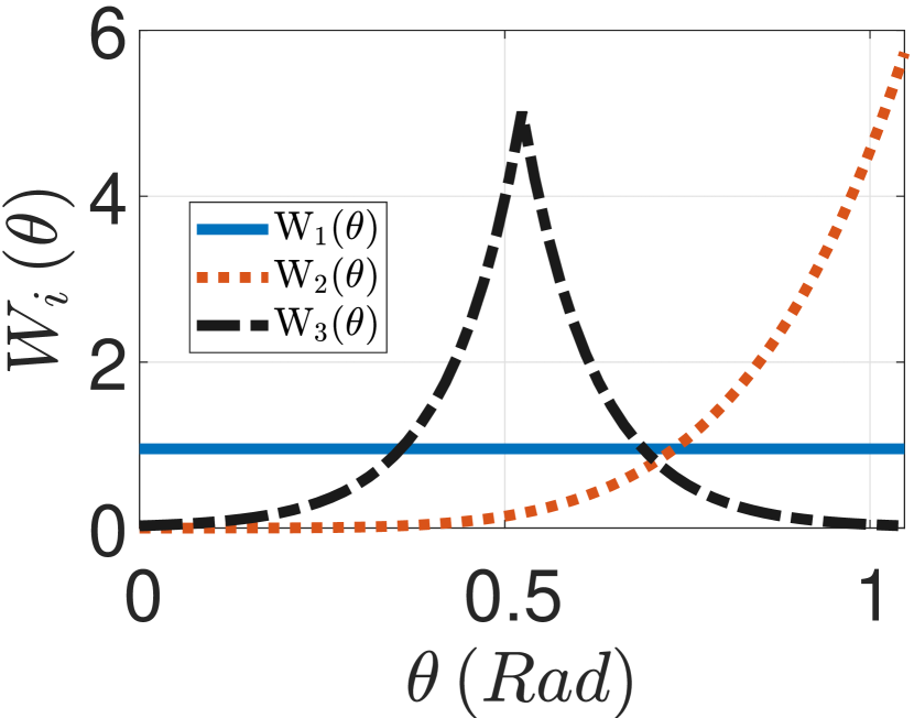
(a)

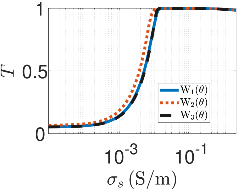
(b)

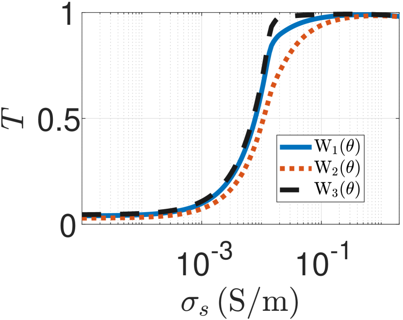
(c)

Figure 2: Tightness of the bound for several weight functions. In accordance with Eq. (2), the ratio is bounded from above by $1$ and is non-negative. The ratio is calculated for a wide range of $\sigma_{\rm{s}}$, while holding all other parameters in Eq. (5) constant. (a) The three weight functions. (b) TE polarization. (c) TM polarization.

It is important to note that the scanning process can be further refined by including additional free-parameters, such as $A$, $\lambda_{\rm{res}}$, $\lambda_{\rm{rel}}$, and $\tau_{\sigma}$ or even to incorporate multiple resonance terms in the Lorentizian model. By exploring different combinations of these parameters, it is possible to identify alternative sets that may also maximize the ratio.

IV Practical Numerical Example - Finite Bandwidth

The discussion in Sec. III aims to verify the tightness of the sum rule in Eq. (2), where an infinite bandwidth is considered. However, in practical systems, absorption performance is typically optimized within a specific bandwidth $\lambda\in[\lambda_{1},\lambda_{2}]$, $\lambda_{1}>0$ and $\lambda_{2}<\infty$. In this section, we present a practical numerical example where we optimize the absorption performance of a Dallenbach absorber with thickness $d=0.4[\rm{m}]$ via the formulations in Eqs. (3) and (4) over a finite bandwidth of $[\lambda_{1},\lambda_{2}]=[0.1,3][\rm{m}]$, while, first, considering a uniform weight function of $W(\theta)=W_{1}(\theta)$ within the angular range of $[\theta_{1},\theta_{2}]=[0,\pi/3]$. This implies that we maximize the contribution within the desired bandwidth, while simultaneously minimizing it outside. Due to the polarization sensitivity of the design, the optimization process is performed separately for TE and TM polarizations. The optimization process that we consider allows also for the design of a stratified inhomogeneous Dallenbach layers. In that case, we consider a piecewise homogeneous design, where, the layer of thickness $d$ is truncated into $N$ parallel sub-layers with identical thickness, each of which is homogeneous (see Fig. 3 for illustration). For any value of $N$ we aim to find optimal design parameters ($\epsilon,\sigma$) that maximizes the tightness, $T$, in Eq. (7). For each sub-layer, we consider the following two models for the design parameters:

• Model $1$ - constant parameters. We use Eq. (5) with $\lambda_{\rm{rel}}=\lambda_{\rm{res}}\approx 0$ and $\frac{2\pi c_{0}\tau_{\sigma}}{\lambda}\ll 1$, resulting in an approximately constant $\epsilon=\epsilon_{0}\epsilon_{r}$ and $\sigma=\sigma_{\rm{s}}$, where $\epsilon_{r}=1+A$ is the relative permittivity. In this model, there are two design parameters, $\epsilon_{r}$ and $\sigma$, which provide only a conductive loss mechanism.

• Model $2$ - frequency dependent parameters. We use Eq. (5) with $\epsilon(\lambda)$ providing three design parameters, $A$, $\lambda_{\rm{rel}}$, and $\lambda_{\rm{res}}$. To reduce the number of design parameters, we set $\sigma_{s}=0$, providing only a polarization loss mechanism.

Model $1$ is widely used in microwave engineering, such as for example in transmission-lines where the parameters usually vary slowly within the desired frequency band to maintain wideband impedance matching. In this model the resonances are typically positioned at much higher frequencies than of interest, as opposed to Model $2$ where they are within (or near the edge) of the operational region. Both models satisfy Karmerts-Kronig relation over the entire infinite frequency range. Note that other models, such as incorporating electric conductivity $\sigma(\lambda)$ in Model $2$ or incorporating multi-resonance polarization response, may also be applicable. However, as the complexity of the model increases, with additional design parameters per sub-layer, the optimization process becomes more involved while the relative improvement decreases.

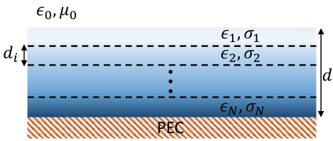
Figure 3: A piecewise homogenous design where the non-magnetic absorbing layer of thickness $d$ is truncated into $N$ parallel sub-layers with identical thickness $d_{i}=d/N$ ($i\in[1,N]$), each of which is homogeneous with $\epsilon_{i},\sigma_{i}$.

The optimization problem to obtain the absorber’s parameters giving the tightest design is non-convex. To solve this optimization problem, we adopt a four-level search approach. First forming a relatively coarse calculation grid. In Model 1 realization, the parameters $\epsilon_{r}$ and $\sigma$ of each layer are uniformly distributed with $M$ points in the rages $0.1\leq\epsilon_{r}\leq 10$ and $0\leq\sigma\leq 0.1\left[\rm{S/m}\right]$. While in Model $2$ realization, the parameters of each layer $A$, $\lambda_{\rm{rel}}$ and $\lambda_{\rm{res}}$ are uniformly distributed with $M$ points in the ranges $0.1\leq A\leq 10$ and $0.1\leq\lambda_{\rm{rel}},\lambda_{\rm{rel}}\leq 10\left[\rm{m}\right]$. Overall, with the parameters of $N$ sub-layers, the total number of calculation grid points in Model $1$ is $M^{2N}$, and for Model $2$ is $M^{3N}$. To ensure memory limitations are not exceeded, for a given $N$, we choose $M$ such to limit the number of grid points to no more than $500$ million. For each calculation grid point, in the first calculation level, we evaluate the cost function in Eq. (3) (or its equivalent in Eq. (4)). In the second step, we focus on the top-performing results from the first-level, coarse grid, calculation step, limiting our search to no more than $0.5\%$ of the total number of grid points. To refine our search further, we perform a local search around each candidate solution of the first-level, evaluating the cost function at steps that are smaller by factor $10$ than in the first-level. Once we have explored possible refinement in the vicinity of the top-performing results of the previous step, the most optimal solution obtained so far is set as an input to the third step. In the third step, we employ a subsequent round of local search, which involves exploring the immediate surroundings of the optimal solution using smaller step sizes, specifically reduced by a factor of $25$ compared to the initial step. This process allows us to fine-tune the optimal solution and achieve even greater refinement. As a final step we perform the optimization procedure described in steps $1-3$ multiple times, adjusting the upper limit of $\epsilon_{r},\lambda_{\rm{rel}},\lambda_{\rm{res}}$ in the first step from $10$ to $3,4.5,7.5$. This step aims to improve the optimized results, as the initial grid points are modified. The entire process is done for both TE and TM polarizations and for several values of $N$. We define a ’parameter of optimality’ $\tau\left(\theta\right)$, as the optimal ratio between the numerator and the denominator integrands in Eq. (4), i.e., the tightness at a specific incident angle as opposed to $T$ in Eq. (7) that is a global tightness,

$$\tau\left(\theta\right)\triangleq\frac{\left|\int_{\lambda_{1}}^{\lambda_{2}}\ln\left|\rho^{\rm{opt}}(\lambda,\theta)\right|\!\,d\lambda\right|}{\rm{RB}\left(\theta\right)},$$ (8)

where $\rho^{\rm{opt}}(\lambda,\theta)$ is the optimal reflection coefficient that was calculated using the optimized parameters. Note that $\rho^{\rm{opt}}(\lambda,\theta)$ and also $\tau\left(\theta\right)$ depend on the weight function $W(\theta)$ via the optimization. By its definition, $\tau\left(\theta\right)$ is bounded between $0$ to $1$ for any $\theta$, where the value $1$ indicates a maximal best (supremum) result that cannot be improved any further. Figure 4 depicts the optimization results for the practical example with $[\lambda_{1},\lambda_{2}]=[0.1,3][\rm{m}]$ and $W(\theta)=W_{1}(\theta)$. Figures 4 (a) and (b) show the optimization results for TE and TM polarizations, respectively, using Model $1$ (with constant parameters) for $N\in[1,7]$. Similarly, Figures 4 (c) and (d) depict the corresponding results for Model $2$ for $N\in[1,4]$ (with frequency-dependent parameters) for TE and TM polarizations, respectively. It can be observed in Fig. 4 that in both models the results at large angles of the TE polarization are better (on average) in comparison to the TM case. This result can be explained by Eq. (1), which shows that for TM polarization the right-hand side of the equation increases infinitely as $\theta$ increases, implying that in order to maintain high values of $\tau\left(\theta\right)$ the left hand side should also grow significantly (without enlarging the finite frequency range of operation). This suggests that at large angles, the primary contribution originate at larger (or smaller) wavelengths that are beyond the range considered in our example. Table I presents the optimal values of the design parameters and the corresponding value of the normalized cost function in Eq. (4) for TE polarization. Results have been rounded and truncated. Similarly, the corresponding results for the TM case are presented in Table II.

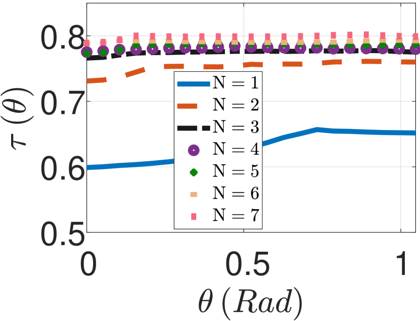
(a)

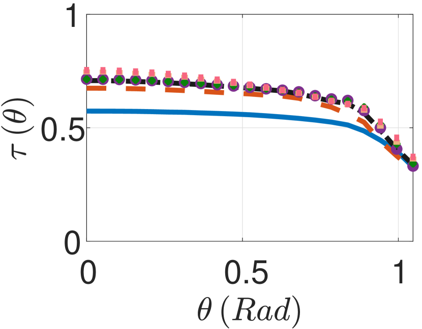
(b)

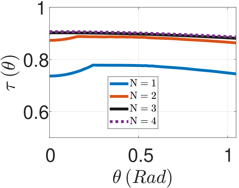
(c)

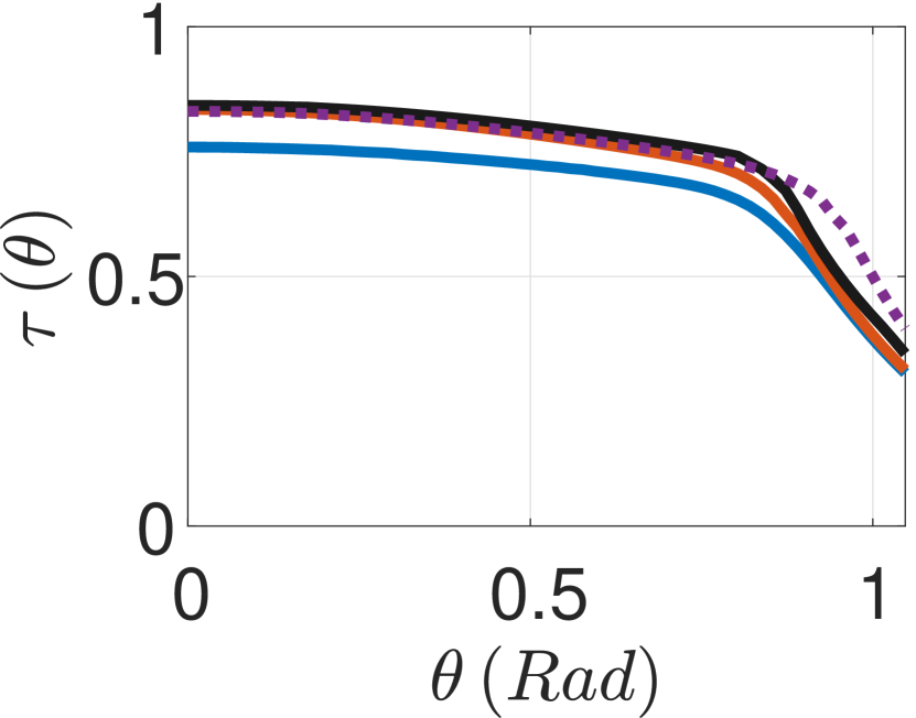
(d)

Figure 4: Optimized results for the practical example with $[\lambda_{1},\lambda_{2}]=[0.1,3][\rm{m}]$ and $W(\theta)=W_{1}(\theta)$. (a) and (b) show the optimized results of the ’parameter of optimality’,$\tau\left(\theta\right)$, for TE and TM polarizations, respectively, using Model $1$ (constant parameters) for $N\in[1,7]$. Similarly, (c) and (d) depict the corresponding results for Model $2$ (with frequency-dependent parameters) for $N\in[1,4]$ for TE and TM polarizations, respectively.

TABLE I: Optimization Results for TE Polarization

	Model $1$ - Optimal $\{\overline{\epsilon}_{r},\overline{\sigma}\}$	Model $1$ - Cost Function	Model $2$ - Optimal $\{\overline{A},\overline{\lambda}_{\rm{rel}},\overline{\lambda}_{\rm{res}}\}$	Model $2$ - Cost Function
		in Eq.(4)		in Eq.(4)
	$\!\!\!\!\!\!\!\!\!\!\!\!\overline{\epsilon}_{r}\!\!=\!\!\{1.45\}\!\!\!\!$		$\!\!\!\!\!\!\!\!\;\;\;\;\overline{A}=\!\!\{3.164\}\!\!\!\!$
$\!\!\!N=1\!\!\!$	$\!\!\!\!\overline{\sigma}\!\!=\!\!\{0.0123\}\!\!\!\!$	$0.6264$	$\!\!\!\!\!\!\!\overline{\lambda}_{\rm{rel}}\!\!=\!\!\{3.05\}\!\!\!\!$	$0.764$
			$\!\!\!\!\!\!\!\overline{\lambda}_{\rm{res}}\!\!=\!\!\{0.01\}\!\!\!\!$
	$\!\!\!\!\overline{\epsilon}_{r}\!\!=\!\!\{2.18,4.03\}\!\!\!\!$		$\!\!\!\!\!\!\!\!\;\;\;\;\overline{A}=\!\!\{0.801,6.947\}\!\!\!\!$
$\!\!\!N=2\!\!\!$	$\!\!\!\!\overline{\sigma}\!\!=\!\!\{0,0.0547\}\!\!\!\!$	$0.7521$	$\!\!\!\!\overline{\lambda}_{\rm{rel}}\!\!=\!\!\{0.553,2.038\}\!\!\!\!$	$0.8805$
			$\!\!\!\!\!\!\!\!\overline{\lambda}_{\rm{res}}\!\!=\!\!\{0.01,0.677\}\!\!\!\!$
	$\!\!\!\!\!\!\!\!\!\!\overline{\epsilon}_{r}\!\!=\!\!\{1.47,2.03,2.72\}\!\!\!\!$		$\!\!\!\!\!\!\!\!\;\;\;\;\overline{A}=\!\!\{0.842,2.946,9.033\}\!\!\!\!$
$\!\!\!N=3\!\!\!$	$\!\!\!\!\overline{\sigma}\!\!=\!\!\{0,0.0164,0.0721\}\!\!\!\!$	$0.7748$	$\!\!\!\!\overline{\lambda}_{\rm{rel}}\!\!=\!\!\{0.223,1.337,1.585\}\!\!\!\!$	$0.8962$
			$\!\!\!\!\!\!\!\!\overline{\lambda}_{\rm{res}}\!\!=\!\!\{0.01,0.347,1.337\}\!\!\!\!$
	$\!\!\!\!\!\!\!\!\!\!\!\!\!\!\!\!\!\!\!\overline{\epsilon}_{r}\!\!=\!\!\{1.88,2.3,3.59,8.43\}\!\!\!\!$		$\!\!\!\!\!\!\!\!\;\;\;\;\overline{A}=\!\!\{1.287,0.01,7.472,8.067\}\!\!\!\!$
$\!\!\!N=4\!\!\!$	$\!\!\!\!\overline{\sigma}\!\!=\!\!\{0,0.0033,0.0289,0.1109\}\!\!\!\!$	$0.7809$	$\!\!\!\!\overline{\lambda}_{\rm{rel}}\!\!=\!\!\{0.345,0.01,1.325,1.447\}\!\!\!\!$	$0.9005$
			$\!\!\!\!\!\!\!\!\!\!\overline{\lambda}_{\rm{res}}\!\!=\!\!\{0.01,0.11,0.01,1.617\}\!\!\!\!$
	$\!\!\!\!\!\!\!\!\!\!\!\!\!\!\!\!\!\!\!\!\!\!\!\!\!\!\!\!\overline{\epsilon}_{r}\!\!=\!\!\{1.8,1.7,3.12,4.86,4.59\}\!\!\!\!$
$\!\!\!N=5\!\!\!$	$\!\!\!\!\overline{\sigma}\!\!=\!\!\{0,0.0025,0.0025,0.0685,0.1125\}\!\!\!\!$	$0.7859$	-	-
	$\!\!\!\!\overline{\epsilon}_{r}\!\!=\!\!\{1.7,1.61,2.49,3.80,4.41,4.75\}\!\!\!\!$
$\!\!\!N=6\!\!\!$	$\!\!\!\!\!\!\!\!\overline{\sigma}\!\!=\!\!\{0,0,0.005,0.0175,0.09,0.1\}\!\!\!\!$	$0.791$	-	-
	$\!\!\!\!\!\!\!\!\!\!\!\!\!\!\!\!\!\!\!\overline{\epsilon}_{r}\!\!=\!\!\{1.57,1.58,1.93,2.88,4.26,4.51,3.67\}\!\!\!\!$
$\!\!\!N=7\!\!\!$	$\!\!\!\overline{\sigma}\!\!=\!\!\{0,0,0.0033,0.0033,0.0367,0.1133,0.0767\}\!\!\!\!$	$0.7982$	-	-

TABLE II: Optimization Results for TM Polarization

	Model $1$ - Optimal $\{\overline{\epsilon}_{r},\overline{\sigma}\}$	Model $1$ - Cost Function	Model $2$ - Optimal $\{\overline{A},\overline{\lambda}_{\rm{rel}},\overline{\lambda}_{\rm{res}}\}$	Model $2$ - Cost Function
		in Eq.(4)		in Eq.(4)
	$\!\!\!\!\!\!\!\!\!\!\!\!\overline{\epsilon}_{r}\!\!=\!\!\{1.51\}\!\!\!\!$		$\!\!\!\!\!\!\!\!\;\;\overline{A}=\!\!\{3.54\}\!\!\!\!$
$\!\!\!N=1\!\!\!$	$\!\!\!\!\overline{\sigma}\!\!=\!\!\{0.0165\}\!\!\!\!$	$0.5217$	$\!\!\!\!\!\!\!\overline{\lambda}_{\rm{rel}}\!\!=\!\!\{2.85\}\!\!\!\!$	$0.6498$
			$\!\!\!\!\!\!\!\overline{\lambda}_{\rm{res}}\!\!=\!\!\{0.01\}\!\!\!\!$
	$\!\!\!\!\!\!\!\!\!\!\!\!\!\!\!\!\!\!\overline{\epsilon}_{r}\!\!=\!\!\{1.96,2.69\}\!\!\!\!$		$\!\!\!\!\!\!\!\!\;\;\overline{A}=\!\!\{1.35,9.896\}\!\!\!\!$
$\!\!\!N=2\!\!\!$	$\!\!\!\!\overline{\sigma}\!\!=\!\!\{0.0063,0.0464\}\!\!\!\!$	$0.5881$	$\!\!\!\!\overline{\lambda}_{\rm{rel}}\!\!=\!\!\{0.777,2.653\}\!\!\!\!$	$0.7015$
			$\!\!\!\!\!\!\!\!\overline{\lambda}_{\rm{res}}\!\!=\!\!\{0.01,0.4126\}\!\!\!\!$
	$\!\!\!\!\!\!\!\!\!\!\overline{\epsilon}_{r}\!\!=\!\!\{2.31,3.44,4.38\}\!\!\!\!$		$\!\!\!\!\!\!\!\!\;\;\;\;\overline{A}=\!\!\{1.09,4.876,10.471\}\!\!\!\!$
$\!\!\!N=3\!\!\!$	$\!\!\!\!\overline{\sigma}\!\!=\!\!\{0,0.0209,0.0918\}\!\!\!\!$	$0.6192$	$\!\!\!\!\overline{\lambda}_{\rm{rel}}\!\!=\!\!\{0.224,1.585,1.982\}\!\!\!\!$	$0.7236$
			$\!\!\!\!\!\overline{\lambda}_{\rm{res}}\!\!=\!\!\{0.01,0.1225,1.514\}\!\!\!\!$
	$\!\!\!\!\!\!\!\!\!\!\!\!\!\!\!\!\!\!\!\overline{\epsilon}_{r}\!\!=\!\!\{2,2.67,3.3,3.72\}\!\!\!\!$		$\!\!\!\!\!\!\!\!\;\;\;\;\overline{A}=\!\!\{1.832,1.288,9.107,8.762\}\!\!\!\!$
$\!\!\!N=4\!\!\!$	$\!\!\!\!\overline{\sigma}\!\!=\!\!\{0,0.011,0.037,0.114\}\!\!\!\!$	$0.6255$	$\!\!\!\!\!\!\!\overline{\lambda}_{\rm{rel}}\!\!=\!\!\{0.44,2.515,1.405,1.382\}\!\!\!\!$	$0.7328$
			$\!\!\!\!\!\!\!\!\overline{\lambda}_{\rm{res}}\!\!=\!\!\{0.01,1.477,0.267,1.985\}\!\!\!\!$
	$\!\!\!\!\!\!\!\!\!\!\!\!\!\!\!\!\!\!\!\!\!\!\!\!\overline{\epsilon}_{r}\!\!=\!\!\{2,2.72,3.4,3.75,4.48\}\!\!\!\!$
$\!\!\!N=5\!\!\!$	$\!\!\!\!\overline{\sigma}\!\!=\!\!\{0,0.0033,0.024,0.053,0.138\}\!\!\!\!$	$0.629$	-	-
	$\!\!\!\!\overline{\epsilon}_{r}\!\!=\!\!\{2.39,0.96,3.64,5.15,4.78,3.91\}\!\!\!\!$
$\!\!\!N=6\!\!\!$	$\!\!\!\!\!\!\!\!\overline{\sigma}\!\!=\!\!\{0,0.0005,0,0.03,0.107,0.14\}\!\!\!\!$	$0.6368$	-	-
	​​​​$\hskip 14.22636pt\overline{\epsilon}_{r}\!\!=\!\!\{2.46,0.9,2.85,4.96,6.24,4.4,4.56\}\!\!\!\!\hskip 14.22636pt$
$\!\!\!N=7\!\!\!$	$\!\!\!\!\!\!\!\!\!\!\!\overline{\sigma}\!\!=\!\!\{0,0,0,0,0.0637,0.1257,0.1553\}\!\!\!\!$	$0.644$	-	-

IV-A The importance of $W(\theta)$

In Section III, we numerically demonstrated that the sum rule in Eq. (2) is tight for several different choices of the weight function $W\left(\theta\right)$, when performing an integration over the entire frequency bandwidth. However, close inspection of Fig. 2 shows weak variations with respect to $W\left(\theta\right)$, indicating that the results are relatively insensitive to the choice of the weight function. This observation may raise doubts about the significance of selecting the weight function $W(\theta)$, as similar parameters lead to a tight sum rule irrespective of the choice of $W(\theta)$. However, in this section, we demonstrate that the situation is different for practical systems that operate within a finite bandwidth. Namely, we investigate how the design parameters are influenced when integrating over a finite bandwidth as can be encountered in practical systems. To this end, we use the same parameters as in the previous practical example (as in Sec. IV) and design two types of layers: a homogenized layer with $N=1$ and a truncated layer with $N=2$. Both of these layers consist of constant parameters (Model 1). We then repeat the optimization process for the weight functions $W_{1}(\theta)$, $W_{2}(\theta)$, and $W_{3}(\theta)$ with $[\lambda_{1},\lambda_{2}]=[0.1,3][\rm{m}]$ for both TE and TM polarizations. Figure 5 (a) shows the optimized results for TE polarization with $N=1$, Figure 5 (b) shows the optimized results for TM polarization with $N=1$, Figure 5 (c) shows the optimized results for TE polarization with $N=2$ and Figure 5 (d) shows the optimized results for TM polarization with $N=2$. Fig. 5 shows that $\tau\left(\theta\right)$ is affected by the choice of $W\left(\theta\right)$. Note that the blue lines in Figs. 5 (a)-(d) represent $W_{1}(\theta)$ cases for $N=1,N=2$. Therefore, the blue lines in Figs. 4 (a) and (b) and Figs. 5 (a) and (b) are identical, respectively ($N=1$). Similarly, the blue lines in Figs. 5 (c) and (d) are identical to the red dashed line in Figs. 4 (a) and (b) ($N=2$). It can be observed by comparing Figs. 5 (a) and (c) with Figs. 5 (b) and (d) that $W_{2}(\theta)$ achieves the highest score for TE polarization, whereas it yields the lowest score for TM polarization. To provide a comprehensive view, the optimized design parameters, ($\epsilon_{r},\sigma$), are listed in Table III for each weight function in both polarizations. Table III indicates that the optimized design parameters vary with the choice of the weight function. This implies that as opposed to the theoretical simulations in Sec. III, when designing a practical Dallenbach absorber that operate within a specific bandwidth, the optimization process should be performed with respect to a specific $W\left(\theta\right)$.

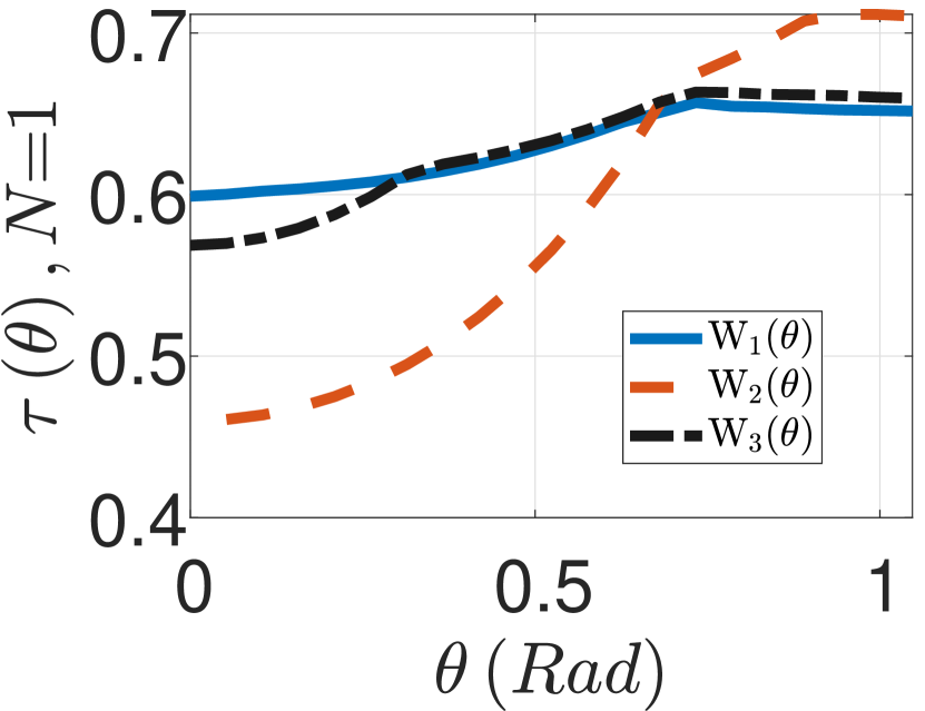
(a)

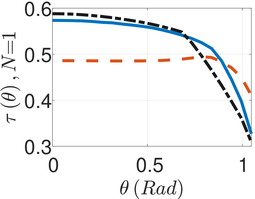
(b)

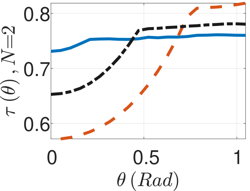
(c)

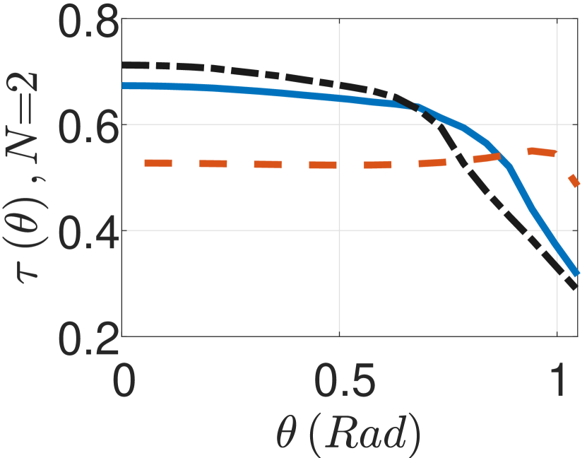
(d)

Figure 5: $\tau\left(\theta\right)$ for homogenized Dallenbach layer ($N=1$) and a truncated layer with $N=2$ for different weight functions $W_{1}(\theta),W_{2}(\theta)$ and $W_{3}(\theta)$ with $[\lambda_{1},\lambda_{2}]=[0.1,3][\rm{m}]$. (a) $N=1$, TE polarization. (b) $N=1$, TM polarization. (c) $N=2$, TE polarization. (d) $N=2$, TM polarization.

TABLE III: The Importance of $W(\theta)$ in Uniform Layers

	Optimized design	Optimized design
	parameters TE	parameters TM
$N\!\!=\!\!1$	$\!\!\!\!\overline{\epsilon}_{r}\!\!=\!\!\{1.4568\}\!\!$	$\!\!\overline{\epsilon}_{r}\!\!=\!\!\{1.5149\}\!\!$
$W_{1}(\theta)$	$\!\!\overline{\sigma}\!\!=\!\!\{0.0123\}\!\!$	$\overline{\sigma}\!\!=\!\!\{0.0165\}\!\!$
$N\!\!=\!\!1$	$\!\!\!\!\overline{\epsilon}_{r}\!\!=\!\!\{1.4024\}\!\!$	$\!\!\!\!\!\!\!\!\overline{\epsilon}_{r}\!\!=\!\!\{2.31\}\!\!$
$W_{2}(\theta)$	$\!\!\overline{\sigma}\!\!=\!\!\{0.0096\}\!\!$	$\overline{\sigma}\!\!=\!\!\{0.0204\}\!\!$
$N\!\!=\!\!1$	$\!\!\!\!\overline{\epsilon}_{r}\!\!=\!\!\{1.5512\}\!\!$	$\!\!\overline{\epsilon}_{r}\!\!=\!\!\{1.4224\}\!\!$
$W_{3}(\theta)$	$\!\!\overline{\sigma}\!\!=\!\!\{0.0118\}\!\!$	$\overline{\sigma}\!\!=\!\!\{0.0144\}\!\!$
$N\!\!=\!\!2$	$\!\!\overline{\epsilon}_{r}\!\!=\!\!\{2.18,4.03\}\!\!$	$\!\!\!\!\!\!\!\!\!\!\!\!\!\!\overline{\epsilon}_{r}\!\!=\!\!\{1.96,2.69\}\!\!$
$W_{1}(\theta)$	$\!\!\overline{\sigma}\!\!=\!\!\{0,0.0547\}\!\!$	$\overline{\sigma}\!\!=\!\!\{0.0063,0.0464\}\!\!$
$N\!\!=\!\!2$	$\!\!\overline{\epsilon}_{r}\!\!=\!\!\{1.73,2.88\}\!\!$	$\!\!\!\!\!\!\!\!\!\!\!\!\!\!\overline{\epsilon}_{r}\!\!=\!\!\{2.86,3.03\}\!\!$
$W_{2}(\theta)$	$\!\!\overline{\sigma}\!\!=\!\!\{0,0.0406\}\!\!$	$\overline{\sigma}\!\!=\!\!\{0.0121,0.0553\}\!\!$
$N\!\!=\!\!2$	$\!\!\!\!\!\!\!\!\!\!\!\!\!\!\!\!\overline{\epsilon}_{r}\!\!=\!\!\{1.88,3.25\}\!\!$	$\!\!\!\!\!\!\!\!\!\!\!\!\!\!\overline{\epsilon}_{r}\!\!=\!\!\{1.95,3.01\}\!\!$
$W_{3}(\theta)$	$\!\!\overline{\sigma}\!\!=\!\!\{0.0005,0.0478\}\!\!$	$\!\!\!\!\!\!\overline{\sigma}\!\!=\!\!\{0.0037,0.05\}\!\!$

V Conclusion

In this work, we presented a sum rule bound for Dallenbach layers subjected to a continuous weighted angular spectrum of oblique incidence plane waves with TE or TM polarizations. We showed that the sum rule is tight when an infinite bandwidth is considered. Moreover, we presented a practical example of designing an optimal absorber operating within a finite bandwidth and specific angular range for both TE and TM cases. By numerically solving an optimization problem, we obtained the design parameters for a piecewise inhomogeneous stratified absorber as a function of the number of sub-layers. Finally, we demonstrated that the optimized design parameters are sensitive to the choice of angular weight function when considering a finite bandwidth.

References

- [1] G. Ruck, Radar Cross Section Handbook. Springer, 1970.
- [2] C. Sohl, M. Gustafsson, and G. Kristensson, “Physical limitations on metamaterials: restrictions on scattering and absorption over a frequency interval,” Journal of Physics D: Applied Physics, vol. 40, no. 22, pp. 7146–7151, 2007.
- [3] N. I. Landy, S. Sajuyigbe, J. J. Mock, D. R. Smith, and W. J. Padilla, “Perfect Metamaterial Absorber,” Physical Review Letters, vol. 100, no. 20, 2008.
- [4] C. Sohl, C. Larsson, M. Gustafsson, and G. Kristensson, “A scattering and absorption identity for metamaterials: Experimental results and comparison with theory,” Journal of Applied Physics, vol. 103, no. 5, p. 054906, 2008.
- [5] Y. Ra’di C.R. Simovski, and S.A. Tretyakov, “Thin Perfect Absorbers for Electromagnetic Waves: Theory, Design, and Realizations,” Physical Review Applied, vol. 3, no. 3, 2015.
- [6] D. E. Fernandes and M. G. Silveirinha, “Topological Origin of Electromagnetic Energy Sinks,” Physical Review Applied, vol. 12, no. 1, 2019.
- [7] A. Krasnok, D. Baranov, H. Li, M.-A. Miri, F. Monticone, and A. Alù, “Anomalies in light scattering,” Advances in Optics and Photonics, vol. 11, no. 4, p. 892, 2019.
- [8] M. Gustafsson, K. Schab, L. Jelinek, and M. Capek, “Upper bounds on absorption and scattering,” New Journal of Physics, vol. 22, no. 7, p. 073013, 2020.
- [9] K. Schab, A. Rothschild, K. Nguyen, M. Capek, L. Jelinek, and M. Gustafsson, “Trade-offs in absorption and scattering by nanophotonic structures,” Optics Express, vol. 28, no. 24, p. 36584, 2020.
- [10] S. Qu and P. Sheng, “Microwave and Acoustic Absorption Metamaterials,” Physical Review Applied, vol. 17, no. 4, 2022.
- [11] M. I. Abdelrahman and F. Monticone, “How Thin and Efficient Can a Metasurface Reflector Be? Universal Bounds on Reflection for Any Direction and Polarization,” Advanced Optical Materials, vol. 11, no. 4, p. 2201782, 2022.
- [12] D. Ye et al., “Ultrawideband Dispersion Control of a Metamaterial Surface for Perfectly-Matched-Layer-Like Absorption,” Physical Review Letters, vol. 111, no. 18, 2013.
- [13] Z. Cao et al., “Backend-Balanced-Impedance Concept for Reverse Design of Ultra-Wideband Absorber,” IEEE Transactions on Antennas and Propagation, vol. 70, no. 11, pp. 11217–11222, 2022.
- [14] A. Parameswaran, A. A. Ovhal, D. Kundu, H. S. Sonalikar, J. Singh, and D. Singh, “A Low-Profile Ultra-Wideband Absorber Using Lumped Resistor-Loaded Cross Dipoles With Resonant Nodes,” IEEE Transactions on Electromagnetic Compatibility, vol. 64, no. 5, pp. 1758–1766, 2022.
- [15] Z.-C. Lin, Y. Zhang, L. Li, Y.-T. Zhao, J. Chen, and K.-D. Xu, “Extremely Wideband Metamaterial Absorber Using Spatial Lossy Transmission Lines and Resistively Loaded High Impedance Surface,” IEEE Transactions on Microwave Theory and Techniques, pp. 1–10, 2023.
- [16] C. L. Holloway, R. R. DeLyser, R. F. German, P. McKenna, and M. Kanda, “Comparison of electromagnetic absorber used in anechoic and semi-anechoic chambers for emissions and immunity testing of digital devices,” IEEE Transactions on Electromagnetic Compatibility, vol. 39, no. 1, pp. 33–47, 1997.
- [17] B.-K. . Chung and H.-T. . Chuah, “Modeling of RF Absorber for Application in the Design of Anechoic Chamber,” Progress In Electromagnetics Research, vol. 43, pp. 273–285, 2003.
- [18] C. Méjean et al., “Electromagnetic absorber composite made of carbon fibers loaded epoxy foam for anechoic chamber application,” Materials Science and Engineering: B, vol. 220, pp. 59–65, 2017
- [19] Y. Arien, P. Dixon, M. Khorrami, A. Degraeve, and D. Pissoort, “Study on the reduction of heatsink radiation by combining grounding pins and absorbing materials,” 2015 IEEE International Symposium on Electromagnetic Compatibility (EMC), 2015.
- [20] J. Xing et al., “Ultra-Thin SSPP-Based Sheet for Suppressing Microwave Radiated Emission in SiP Modules,” IEEE Transactions on Electromagnetic Compatibility, vol. 65, pp. 1–10, 2022.
- [21] A. Khoshniat and R. Abhari, “Metamaterial Absorbers for Lining System Shield Box and Packaging: Cavity Analysis and Equivalent Material Design,” IEEE Transactions on Electromagnetic Compatibility, vol. 63, no. 4, pp. 1007–1014, 2021.
- [22] C. Hägglund and S. P. Apell, “Plasmonic Near-Field Absorbers for Ultrathin Solar Cells,” The Journal of Physical Chemistry Letters, vol. 3, no. 10, pp. 1275–1285, 2012.
- [23] B. Mulla and C. Sabah, “Perfect metamaterial absorber design for solar cell applications,” Waves in Random and Complex Media, vol. 25, no. 3, pp. 382–392, 2015.
- [24] K. N. Rozanov, “Ultimate thickness to bandwidth ratio of radar absorbers,” IEEE Transactions on Antennas and Propagation, vol. 48, no. 8, pp. 1230–1234, 2000.
- [25] H. Li and A. Alù, “Temporal switching to extend the bandwidth of thin absorbers,” Optica, vol. 8, no. 1, p. 24, 2020.
- [26] Z. Hayran, A. Chen, and F. Monticone, “Spectral causality and the scattering of waves,” Optica, vol. 8, no. 8, p. 1040, 2021.
- [27] C. Firestein, A. Shlivinski, and Y. Hadad, “Absorption and Scattering by a Temporally Switched Lossy Layer: Going beyond the Rozanov Bound,” Physical Review Applied, vol. 17, no. 1, 2022.
- [28] C. Firestein, A. Shlivinski, and Y. Hadad, “Sum Rule Bounds Beyond Rozanov Criterion in Linear and Time-Invariant Thin Absorbers,” arXiv:2210.06949 [physics], 2022.
- [29] J. P. Doane, K. Sertel, and J. L. Volakis, “Matching bandwidth limits for arrays backed by a conducting ground plane,” IEEE Trans. Antennas Propag., vol. 61, no. 5, pp. 2511–2518, 2013.
- [30] J. P. Doane, K. Sertel, and J. L. Volakis, “Bandwidth Limits for Lossless, Reciprocal PEC-backed Arrays of Arbitrary Polarization,” IEEE Transactions on Antennas and Propagation, vol. 62, no. 5, pp. 2531–2542, 2014.
- [31] M. H. Novak, F. A. Miranda, and J. L. Volakis, “Ultra-Wideband Phased Array for Millimeter-Wave ISM and 5G Bands, Realized in PCB,” IEEE Transactions on Antennas and Propagation, vol. 66, no. 12, pp. 6930–6938, 2018.
- [32] J. Zhong, A. Johnson, E. A. Alwan, and J. L. Volakis, “Dual-Linear Polarized Phased Array With 9:1 Bandwidth and 60° Scanning Off Broadside,” IEEE Transactions on Antennas and Propagation, vol. 67, no. 3, pp. 1996–2001, 2019.
- [33] R. B. Adler, L. J. Chu, and R. M. Fano, Electromagnetic Energy Transmission and Radiation, Hoboken, NJ, USA: Wiley, 1968.
- [34] R. E. Collin, Foundations for Microwave Engineering. McGraw-Hill, New York, 1966.
- [35] D. M. Pozar, Microwave Engineering. 4th ed. John Wiley Sons, Hoboken, NJ, 2011.
- [36] J. D. Jackson, Classical Electrodynamics. John Wiley & Sons, Hoboken, 2007.