Time Fairness in Online Knapsack Problems

Abstract

The online knapsack problem is a classic problem in the field of online algorithms. Its canonical version asks how to pack items of different values and weights arriving online into a capacity-limited knapsack so as to maximize the total value of the admitted items. Although optimal competitive algorithms are known for this problem, they may be fundamentally unfair, i.e., individual items may be treated inequitably in different ways. Inspired by recent attention to fairness in online settings, we develop a natural and practically-relevant notion of time fairness for the online knapsack problem, and show that the existing optimal algorithms perform poorly under this metric. We propose a parameterized deterministic algorithm where the parameter precisely captures the Pareto-optimal trade-off between fairness and competitiveness. We show that randomization is theoretically powerful enough to be simultaneously competitive and fair; however, it does not work well in practice, using trace-driven experiments. To further improve the trade-off between fairness and competitiveness, we develop a fair, robust (competitive), and consistent learning-augmented algorithm with substantial performance improvement in trace-driven experiments.

1 Introduction

The online knapsack problem ($\mathsf{OKP}$) is a well-studied problem in online algorithms. It models a resource allocation process, in which one provider allocates a limited resource (i.e., the knapsack’s capacity) to consumers (i.e., items) arriving sequentially in order to maximize the total return (i.e., optimally pack items subject to the capacity constraint).

In $\mathsf{OKP}$, as in many other online decision problems, there is a trade-off between efficiency, i.e., maximizing the value of the packed items, and fairness, i.e., ensuring equitable “treatment” for different items across some desirable criteria. To illustrate the importance of these considerations in the context of $\mathsf{OKP}$, it is perhaps best to start with an example.

Consider a cloud computing resource accepting heterogeneous jobs online from clients sequentially. Each job includes a bid that the client is willing to pay, and an amount of resources required to execute it. The cloud computing resource is limited – there are not enough resources to service all of the incoming requests. We define the quality of a job as the ratio of the bid price paid by the client to the quantity of resources required for it.

How do we algorithmically solve the problem posed in Example 1? Note that the limit on the resource implies that the problem of accepting and rejecting items reduces precisely to the online knapsack problem. If we cared only about the overall quality of accepted jobs, we would intuitively be solving the unconstrained online knapsack problem. However, at the same time, it might be desirable for an algorithm to apply the same quality criteria to each job that arrives. As we will show in §3, existing optimal algorithms for online knapsack do not fulfill this second requirement. In particular, although two jobs may have a priori identical quality, the optimal algorithm discriminates between them based on their arrival time in the online queue: a typical job, therefore, may have a higher chance of being accepted if it happens to arrive earlier rather than later. Preventing these kinds of choices while still maintaining competitive standards of overall quality will form this work’s focus.

Precursors to this work. $\mathsf{OKP}$ was first studied in [Marchetti:95], with important optimal results following in [ZCL:08]. Recent work [sentinel21, Zeynali:21, Bockenhauer:14] has explored this problem with additional information and/or learning augmentation, which we also consider. In the context of fairness, our work is most closely aligned with the notions of time fairness recently studied for prophet inequalities [arsenis22] and the secretary problem [Buchbinder:09], which considered stochastic and random order input arrivals. To the best of our knowledge, our work is the first to consider any notions of fairness in $\mathsf{OKP}$, which considered the adversarial input arrivals. We present a comprehensive review of related studies on the knapsack problem and fairness in Appendix 2.

Our contributions. First, we formalize a natural notion of time-independent fairness (introduced by [arsenis22]) in the context of $\mathsf{OKP}$. Through impossibility results (Thms. 4.1, 4.1, 4.1), we show that this notion is too restrictive, and motivate a revised definition which is feasible for $\mathsf{OKP}$. We design a deterministic algorithm to achieve the desired fairness properties and show that it captures the Pareto-optimal trade-off between fairness and competitiveness (Thms. 5.1, 5.1). We further investigate randomization, showing that a randomized algorithm can optimize both competitive ratio and fairness in theory (Thm. 3, Prop. 5.2); however, in trace-driven experiments, randomization underperforms significantly. Motivated by this observation, we incorporate predictions to simultaneously improve fairness and competitiveness. We introduce a fair, deterministic learning-augmented algorithm with bounded consistency and robustness (Thms. 5.3, 5.3). Finally, we present empirical results evaluating our proposed algorithms on real-world cloud traces for the online job scheduling problem.

Our research introduces three primary technical contributions. First, we develop a novel definition of $\alpha$-conditional time-independent fairness. This notion of fairness, which is generalizable to many online problems, captures a natural perspective on fairness in online settings. Second, we present a constructive lower-bound technique to derive a Pareto-optimal trade-off between fairness and competitiveness, illustrating the inherent challenges in this problem. This result provides a strong understanding of the necessary compromise between fair decision-making and efficiency in $\mathsf{OKP}$, and gives insight into time fairness results achievable in other online problems. Lastly, we propose a novel weak prediction model inspired by the offline approximation algorithms literature. Like our notion of fairness, this prediction model is generalizable to other online problems, and our results suggest that even simple accurate predictions can concurrently improve an online algorithm’s fairness and performance.

2 Related Work

We consider the online knapsack problem ($\mathsf{OKP}$), a classical resource allocation problem wherein items with different weights and values arrive sequentially, and we wish to admit them into a capacity-limited knapsack, maximizing the total value subject to the capacity constraint.

Our work contributes to several active lines of research, including a rich literature on $\mathsf{OKP}$ first studied in [Marchetti:95], with important optimal results following in [ZCL:08]. In the past several years, research in this area has surged, with many works considering variants of the problem, such as removable items [Cygan:16], item departures [sun2022online], and generalizations to multidimensional settings [Yang2021Competitive]. Closest to this work, several studies have considered the online knapsack problem with additional information or in a learning-augmented setting, including frequency predictions [sentinel21], online learning [Zeynali:21], and advice complexity [Bockenhauer:14].

In the literature on the knapsack problem, fairness has been recently considered in [Patel:20] and [Fluschnik:19]. Unlike our work, both deal exclusively with the standard offline setting of knapsack, and consequently do not consider time fairness. [Patel:20] introduces a notion of group fairness for the knapsack problem, while [Fluschnik:19] introduces three notions of “individually best, diverse, and fair” knapsacks which aggregate the voting preferences of multiple voters. To the best of our knowledge, our work is the first to consider notions of fairness in the online knapsack problem.

In the broader literature on online algorithms and dynamic settings, several studies explore fairness, although most consider notions of fairness that are different from the ones in our work. Online fairness has been explored in resource allocation [Manshadi:21, Sinclair:20, Bateni:16, Sinha:23], fair division [Kash:13], refugee assignment [Freund:23], matchings [Deng:23, Ma:22], prophet inequalities [Correa:21], organ allocation [Bertsimas:13], and online selection [Benomar:23]. [Banerjee:22] shows competitive algorithms for online resource allocation which seek to maximize the Nash social welfare, a metric which quantifies a trade-off between fairness and performance. [Deng:23] also explicitly considers the intersection between predictions and fairness in the online setting. In addition to these problems, there are also several online problems adjacent to $\mathsf{OKP}$ in the literature which would be interesting to explore from a fairness perspective, including one-way trading [ElYaniv:01, sun2022online], bin packing [Balogh:17:BP, Johnson:74:BP], and single-leg revenue management [Balseiro:22, Ma:21].

In the online learning literature, several works consider fairness using regret as a performance metric. In particular, [Talebi:18] studies a stochastic multi-armed bandit setting where tasks must be assigned to servers in a proportionally fair manner. Several other works including [Baek:21:MAB, Patil:21:MAB, Chen:20:MAB] build on these results using different notions of fairness. For a general resource allocation problem, [Sinha:23] presents a fair online resource allocation policy achieving sublinear regret with respect to an offline optimal allocation. Furthermore, many works in the regret setting explicitly consider fairness from the perspective of an $\alpha$-fair utility function, including [Sinha:23, Si:22:alpha, Wang:22:alpha] , which partially inspires our parameterized definition of $\alpha$-CTIF (Def. 4.2).

In the broader ML research community, fairness has seen burgeoning recent interest, particularly from the perspective of bias in trained models. Mirroring the literature above, multiple definitions of fairness in this setting have been proposed and studied, including equality of opportunity [Hardt:16:ML], conflicting notions of fairness [Kleinberg:17:ML], and inherent trade-offs between performance and fairness constraints [Bertsimas:12]. Fairness has also been extensively studied in impact studies such as [Chouldechova:17:ML], which demonstrated the disparate impact of recidivism prediction algorithms used in the criminal justice system on different demographics.

3 Problem & Preliminaries

Problem formulation. In the online knapsack problem ($\mathsf{OKP}$), we have a knapsack (resource) with capacity $B$ and items arriving online. We denote an instance $\mathcal{I}$ of $\mathsf{OKP}$ as a multiset of $n$ items, where each item has a value and a weight. Formally, $\mathcal{I}=\left[(v_{j},w_{j})_{j=1}^{n}\right]$.We assume that $v_{j}$ and $w_{j}$ correspond to the value and weight respectively of the $j$th item in the arrival sequence, where $j$ also denotes the arrival time of this item. We denote by $\Omega$ the set of all feasible input instances.

The objective in $\mathsf{OKP}$ is to accept items into the knapsack to maximize the sum of values while not violating the capacity limit of $B$. As is standard in the literature on online algorithms, at each time step $j$, the algorithm is presented with an item, and must immediately decide whether to accept it ($x_{j}=1$) or reject it ($x_{j}=0$). The offline version of $\mathsf{OKP}$ (i.e., $\mathsf{Knapsack}$) is a classical combinatorial problem with strong connections to resource allocation. It can be summarized as $\max\sum_{j=1}^{n}v_{j}x_{j},\;\;\text{s.t.}\;\;\sum_{j=1}^{n}w_{j}x_{j}\leq~{}B,\;\;x_{j}\in\{0,1\}\text{ for all }j\in[n].$

$\mathsf{Knapsack}$ is a canonical NP-complete problem (strongly NP-complete for non-integral inputs [strongNPC]). There is a folklore pseudopolynomial algorithm known for the exact problem. $\mathsf{Knapsack}$ is one of the hardest but most ubiquitous problems arising in applications today.

Competitive analysis. $\mathsf{OKP}$ has been extensively studied under the framework of competitive analysis, where the goal is to design an online algorithm that maintains a small competitive ratio [Borodin:92], i.e., performs nearly as well as the offline optimal algorithm. For an online algorithm $\mathsf{ALG}$ and an offline algorithm $\mathsf{OPT}$, the competitive ratio for a problem with a maximization objective is defined as $\max_{\mathcal{I}\in\Omega}\mathsf{OPT}(\mathcal{I})/\mathsf{ALG}(\mathcal{I})$, where $\mathsf{OPT}(\mathcal{I})$ is the optimal profit on the input $\mathcal{I}$, and $\mathsf{ALG}(\mathcal{I})$ is the profit obtained by the online algorithm on this input. The competitive ratio is always at least one, and the lower it is, the better the algorithm.

Assumptions and additional notation. We assume that the set of value densities $\{v_{j}/w_{j}\}_{j\in[n]}$ has bounded support, i.e., $v_{j}/w_{j}\in[L,U]$ for all $j$, where $L$ and $U$ are known. These are standard assumptions in the literature for many online problems, including $\mathsf{OKP}$, one-way trading, and online search; without them, the competitive ratio of any online algorithm is unbounded [Marchetti:95, ZCL:08]. We also adopt a second assumption from the literature on $\mathsf{OKP}$, assuming that the weight of each individual item is sufficiently small compared to the knapsack’s capacity, which is typically reasonable in practice [ZCL:08]. This is a mild assumption that is necessary for any meaningful result. For the rest of this paper, we will assume WLOG that $B=1$. We can scale everything down by a factor of $B$ otherwise. We let $z_{j}\in[0,1]$ denote the knapsack utilization when the $j$th item arrives, i.e. the fraction of the knapsack’s total capacity that is currently filled with previously accepted items.

Existing results. Prior work on $\mathsf{OKP}$ has resulted in an optimal deterministic algorithm for the problem described above, shown by ZCL:08 in a seminal work using the framework of online threshold-based algorithms (OTA). In OTA, a carefully designed threshold function is used to facilitate the decisions made at each time step. This threshold is specifically designed such that greedily accepting inputs whose values meet or exceed the threshold at each step provides a competitive guarantee. This algorithmic framework has seen success in the related online search and one-way trading problems [Lee:22, Sun:21, Lorenz:08, ElYaniv:01] as well as $\mathsf{OKP}$ [ZCL:08, sun2022online, Yang2021Competitive].

The $\mathsf{ZCL}$ algorithm: The algorithm shown by ZCL:08 is a deterministic threshold-based algorithm that achieves a competitive ratio of $\ln(\nicefrac{{U}}{{L}})+1$; they also show that this is the optimal competitive ratio for any deterministic or randomized algorithm. We henceforth refer to this algorithm as the $\mathsf{ZCL}$ algorithm. In the $\mathsf{ZCL}$ algorithm, items are admitted based on the monotonically increasing threshold function $\Phi(z)=\left(\nicefrac{{Ue}}{{L}}\right)^{z}\left(\nicefrac{{L}}{{e}}\right)$, where $z\in[0,1]$ is the current utilization (see Fig. 2(a)). The $j$th item in the sequence is accepted iff it satisfies $v_{j}/w_{j}\geq\Phi(z_{j})$, where $z_{j}$ is the utilization at the time of the item’s arrival. This algorithm is optimally competitive [ZCL:08, Thms. 3.2, 3.3].

4 Time Fairness

In Example 1, the constraint that was infringed was one of time fairness. In this section, inspired by prior work [arsenis22] which explores the concept of time fairness in the context of prophet inequalities, we formally define the notion in the context of $\mathsf{OKP}$. We relegate formal proofs to Appendix 4.1.

4.1 Time-Independent Fairness (TIF)

In Example 1, it is reasonable to ask that the probability of an item’s admission into the knapsack depend solely on its value density $x$, and not on its arrival time $j$. This is a natural generalization to $\mathsf{OKP}$ of the time-independent fairness constraint, proposed in [arsenis22]. [Time-Independent Fairness (TIF) for $\mathsf{OKP}$]

An $\mathsf{OKP}$ algorithm $\mathsf{ALG}$ is said to satisfy TIF if there exists a function $p:[L,U]\rightarrow[0,1]$ such that:

$$\Pr\left[\mathsf{ALG}\text{ accepts }j\text{th item in }\mathcal{I}\;\lvert\;v_{j}/w_{j}=x\right]=p(x),\;\text{ for all }\mathcal{I}\in\Omega,j\in[n],x\in[L,U].$$

In other words, the probability of admitting an item of value density $x$ depends only on $x$, and not on its arrival time. Note that this definition makes sense only in the online setting. We start by noting that the $\mathsf{ZCL}$ algorithm is not TIF.

The $\mathsf{ZCL}$ algorithm [ZCL:08] is not TIF.

Proof.

Let $z_{j}\in[0,1]$ be the knapsack’s utilization when the $j$th item arrives. When the knapsack is empty, $z_{j}=0$, and when the knapsack is close to full, $z_{j}=1-\epsilon$ for some small $\epsilon>0$. Pick any instance with sufficiently many items, and pick $z_{A}<z_{B}$ such that at least one admitted item, say the $k$th one, satisfies $\Phi(z_{A})\leq v_{k}<\Phi(z_{B})$. Note that this implies that the $k$th item arrived between the utilization being at $z_{A}$ and at $z_{B}$. Now, modify this same instance by adding a copy of the $k$th item after the utilization has reached $z_{B}$. Note that this item now has probability zero of being admitted. This implies that two items with the same value-to-weight ratio have different probabilities of being admitted into the knapsack, contradicting the definition of TIF. ∎

We seek to design an algorithm for $\mathsf{OKP}$ that satisfies TIF while being competitive against an optimal offline solution. Given Observation 4.1, a natural question is whether any such algorithm exists that maintains a bounded competitive ratio. Of course, the trivial algorithm which rejects all items is TIF, as the probability of accepting any item is zero. We now show that there is no other algorithm for $\mathsf{OKP}$ that achieves our desired conditions simultaneously.

[] There is no nontrivial algorithm for $\mathsf{OKP}$ that guarantees TIF without additional information about the input.

Proof.

WLOG assume that all items have the same value density $x=L=U$. Assume for the sake of a contradiction that there is some algorithm $\mathsf{ALG}$ which guarantees TIF, and suppose we have a instance $\mathcal{I}$ with $n$ items (which we will set later).

Since we assume that $\mathsf{ALG}$ guarantees TIF, consider $p(x)$, the probability of admitting an item with value density $x$. Let $p(x)=\texttt{p}$. Note that $\texttt{p}>0$, and also that it cannot depend on the input length $n$. Note that we can have have all items of equal weight $w$, so that for $n\gg 3B/w\texttt{p}$, the knapsack is full with high probability. But now consider modifying the input sequence from $\mathcal{I}$ to $\mathcal{I}^{\prime}$, by appending a copy of itself, i.e., increasing the input with another $n$ items of exactly the same type. The probability of admitting these new items must be (eventually) zero, even though they have the same value-to-weight ratio as the first half of the input (and, indeed, the same weights). Therefore, the algorithm violates the TIF constraint on the instance $\mathcal{I}^{\prime}$, which is a contradiction. ∎

Theorem 4.1 implies that achieving TIF is impossible without leveraging additional information about the input instance. sentinel21 present the first work, to our knowledge, that incorporates ML predictions into $\mathsf{OKP}$. The predictions used in their setting are in the form of frequency predictions, which give upper and lower bounds on the total weight of items with a given value density in the input instance. Formally, for each value density $x$, where $s_{x}:=\sum_{j:v_{j}/w_{j}=x}w_{j}$ is the total weight of items with value density $x$, we get a predicted pair $(\ell_{x},u_{x})$ satisfying $\ell_{x}\leq s_{x}\leq u_{x}$ for all $x\in[L,U]$.

For their analysis, [sentinel21] assumes that the $\mathsf{OKP}$ instance respects these predictions, although it can be adversarial within these bounds. It is conceivable that additional information in the form of either the total number of items or these frequency predictions can enable a nontrivial $\mathsf{OKP}$ algorithm to guarantee TIF. The following two results, however, give negative answers to this idea, even for perfect predictions, i.e., $\ell_{x}=u_{x}=s_{x}$ for all $x\in[L,U]$ (i.e., the algorithm knows each $s_{x}$ in advance).

There is no nontrivial competitive algorithm for $\mathsf{OKP}$ which guarantees TIF, even given perfect frequency predictions as defined in [sentinel21].

Proof.

Again WLOG assume that all items have the same value density $x=L=U$, so that $s_{x}=\sum_{i=1}^{n}w_{i}$. Assume for the sake of a contradiction that there is some competitive algorithm $\mathsf{ALG}^{\texttt{FP}}$ which uses frequency predictions to guarantee TIF.

Since we assume that $\mathsf{ALG}^{\texttt{FP}}$ guarantees TIF, consider $p(x)$, the probability of admitting any item. Let $p(x)=\texttt{p}$. Again, note that $\texttt{p}>0$, and also that it cannot depend on the input length $n$, but can depend on $s_{x}$ this time.

Consider two instances $\mathcal{I}$ and $\mathcal{I}^{\prime}$ as follows: $\mathcal{I}$ consists exclusively of “small” items of (constant) weight $w_{\delta}\ll B$ each, whereas $\mathcal{I}^{\prime}$ consists of a small, constant number of such small items followed by a single “large” item of weight $B-\delta/2$. Note that by taking enough items in $\mathcal{I}$, we can ensure the two instances have the same total weight $s(x)$. Therefore, $p(x)$ must be the same for these two instances, by assumption. Of course, the items all have value $x$ by our original assumption.

Note that the optimal packing in both instances would nearly fill up the knapsack. However, $\mathcal{I}^{\prime}$ has the property that any competitive algorithm must reject all the initial smaller items, as admitting any of them would imply that the large item can no longer be admitted. By making $w_{\delta}$ arbitrarily small, we can make the algorithm arbitrarily non-competitive.

The instance $\mathcal{I}$ guarantees that $p(x)$ is sufficiently large (i.e., bounded below by some constant), and so with high probability, at least one item in $\mathcal{I}^{\prime}$ is admitted within the first constant number of items. Therefore, with high probability, $\mathsf{ALG}^{\texttt{FP}}$ does not admit the large-valued item in $\mathcal{I}^{\prime}$, and so it cannot be competitive. ∎

There is no nontrivial competitive algorithm for $\mathsf{OKP}$ which guarantees TIF, even if the algorithm knows the input length $n$ in advance.

Proof.

Again WLOG assume that all items have the same value density $x=L=U$. Assume for the sake of a contradiction that there is some competitive algorithm $\mathsf{ALG}^{\texttt{N}}$ which uses knowledge of the input length $n$ to guarantee TIF.

We will consider only input sequences of length $n$ (assumed to be sufficiently large), consisting only of items with value density $x$. Again, since we assume that $\mathsf{ALG}^{\texttt{FP}}$ guarantees TIF, consider $p(x)$, the probability of admitting any item. Let $p(x)=\texttt{p}$. Again, note that $\texttt{p}>0$, and also that it must be the same for all input sequences of length $n$.

Consider such an instance $\mathcal{I}$, consisting of identical items of (constant) weight $w_{c}$ each. Suppose the total weight of the items is very close to the knapsack capacity $B$. Since the expected number of items admitted is $n\texttt{p}$, the total value admitted is $x\cdot n\texttt{p}$ on expectation. The optimal solution admits a total value of $nx$ (since the total weight is close to $B$), and therefore, the competitive ratio is roughly $1/\texttt{p}$. Since we assumed the algorithm was competitive, it follows that p must be bounded below by a constant.

Now consider a different instance $\mathcal{I}^{\prime}$, consisting of $3\log(n)/\texttt{p}^{2}$ items of weight $w_{\delta}\ll B$, followed by $n-3\log(n)/\texttt{p}^{2}$ “large” items of weight $B-w_{\delta}/2$. Note that these are well-defined, as p is bounded below by a constant, and $n$ is sufficiently large. The instance $\mathcal{I}^{\prime}$ again has the property that any competitive algorithm must reject all the initial smaller items, as admitting any of them would imply that none of the large items can be admitted.

However, by the coupon collector problem, with high probability ($1-\text{poly}(1/n)$), at least one of the $3\log(n)/\texttt{p}^{2}$ small items is admitted, which contradicts the competitiveness of $ALG^{\texttt{N}}$. As before, by making $w_{\delta}$ arbitrarily small, we can make the algorithm arbitrarily non-competitive. ∎

Theorems 4.1 and 4.1 essentially close off TIF as a feasible candidate for the fairness constraint that can be imposed on competitive algorithms. An algorithm that knows both $n$ and the weights of items in the input is closer in spirit to an offline algorithm than an online one. We remark that [arsenis22, Thm. 6.2] shows a TIF impossibility result in a similar vein, wherein certain secretary problem variants which are forced to hire at least one candidate cannot satisfy TIF.

4.2 Conditional Time-Independent Fairness (CTIF)

Motivated by the results in §4.1, we now present a revised but still natural notion of fairness in Definition 4.2. This notion relaxes the constraint and narrows the scope of fairness to consider items which arrive while the knapsack’s utilization is within a subinterval of the knapsack’s capacity.

[$\alpha$-Conditional Time-Independent Fairness ($\alpha$-CTIF) for $\mathsf{OKP}$] For $\alpha\in[0,1]$, an $\mathsf{OKP}$ algorithm $\mathsf{ALG}$ is said to satisfy $\alpha$-CTIF if there exists a subinterval $\mathcal{A}=[a,b]\subseteq[0,1]$ where $b-a=\alpha$, and a function $p:[L,U]\rightarrow[0,1]$ such that:

$$\Pr\left[\mathsf{ALG}\text{ accepts }j\text{th item in }\mathcal{I}\;\lvert\;\left(v_{j}/w_{j}=x\right)\text{and}\ (z_{j}+w_{j}\in\mathcal{A})\right]=p(x),$$

$$\text{ for all }\mathcal{I}\in\Omega,j\in[n],x\in[L,U].$$

In particular, note that if $\alpha=1$, then $\mathcal{A}=[0,1]$, and any item that arrives while the knapsack still has the capacity to admit it is considered within this definition. In fact, $1$-CTIF is the same as TIF provided that the knapsack has capacity remaining for the item under consideration. Furthermore, the larger the value of $\alpha$, the stronger the notion of fairness, but even the strongest notion of CTIF, namely $1$-CTIF, is strictly weaker than TIF. This notion of fairness circumvents many of the challenges associated with TIF, and is a feasible goal to achieve in the online setting while preserving competitive guarantees. However, we note that the canonical $\mathsf{ZCL}$ algorithm [ZCL:08] still is not $1$-CTIF.

[] The $\mathsf{ZCL}$ algorithm is not 1-CTIF.

Proof.

This follows immediately from the fact that the threshold value in $\mathsf{ZCL}$ changes each time an item is accepted, which corresponds to the utilization changing. Consider two items with the same value density (close to $L$), where one of the items arrives first in the sequence, and the other arrives when the knapsack is roughly half-full, and assume that there is enough space in the knapsack to accommodate both items when they arrive. The earlier item will be admitted with certainty, whereas the later item will with high probability be rejected. So despite having the same value, the items will have a different admission probability purely based on their position in the sequence, violating $1$-CTIF. ∎

Our definition of $\alpha$-CTIF offers a fairness concept that is both achievable for $\mathsf{OKP}$ and potentially adaptable to other online problems, such as online search [Lorenz:08, Lee:22], one-way trading [ElYaniv:01, Sun:21], bin-packing [Balogh:17:BP, Johnson:74:BP], and single-leg revenue management [Ma:21, Balseiro:22]. We are now ready to present our main results, including deterministic, randomized, and learning-augmented algorithms which satisfy $\alpha$-CTIF and provide competitive guarantees.

5 Online Fair Algorithms

Table 1: A summary of key notations.

Notation	Description
$j\in[n]$	Current position in sequence of items
$x_{j}\in\{0,1\}$	Decision for $j$th item. $x_{j}=1$ if accepted, $x_{j}=0$ if not accepted
$U$	Upper bound on the value density of any item
$L$	Lower bound on the value density of any item
$\alpha$	Fairness parameter, defined in Definition 4.2
$w_{j}$	(Online input) Item weight revealed to the player when $j$th item arrives
$v_{j}$	(Online input) Item value revealed to the player when $j$th item arrives

In this section, we start with some simple fairness-competitiveness trade-offs. In §5.1, we develop algorithms that satisfy CTIF constraints while remaining competitive. Finally, we explore the power of randomization in §5.2 and predictions in §5.3 for further performance improvement. For the sake of brevity, we relegate most of the proofs to Appendix 5, but provide proof sketches in a few places. We start with a warm-up result capturing the essence of the inherent trade-offs through an examination of constant threshold-based algorithms for $\mathsf{OKP}$. Such an algorithm sets a single threshold $\phi$ and greedily accepts any items with value density $\geq\phi$.

Any constant threshold-based algorithm for $\mathsf{OKP}$ is $1$-CTIF. Furthermore, any constant threshold-based deterministic algorithm for $\mathsf{OKP}$ cannot be better than $(\nicefrac{{U}}{{L}})$-competitive.

Proof.

Consider an arbitrary threshold-based algorithm $\mathsf{ALG}$ with constant threshold value $\phi$. For any instance $\mathcal{I}$, and any item, say the $j$th one, in this instance, note that the probability of admitting the item depends entirely on the threshold $\phi$, and nothing else, as long there is enough space in the knapsack to admit it. So for any value density $x\in[L,U]$, the admission probability $p(x)$ is just the indicator variable capturing whether there is space for the item or not.

For the second part, given a deterministic $\mathsf{ALG}$ with a fixed constant threshold $\phi\in[L,U]$, there are two cases. If $\phi>L$, the instance $\mathcal{I}$ consisting entirely of $L$-valued items induces an unbounded competitive ratio, as no items are admitted by $\mathsf{ALG}$. If $\phi=L$, consider the instance $\mathcal{I}^{\prime}$ consisting of $m$ equal-weight items with value $L$ followed by $m$ items with value $U$, and take $m$ large enough that the knapsack can become full with only $L$-valued items. $\mathsf{ALG}$ here admits only $L$-valued items, whereas the optimal solution only admits $U$-valued items, and so $\mathsf{ALG}$ cannot do better than the worst-case competitive ratio of $\frac{U}{L}$ for $\mathsf{OKP}$. ∎

How does this trade-off manifest itself in the $\mathsf{ZCL}$ algorithm? We know from Observation 4.2 that $\mathsf{ZCL}$ is not $1$-CTIF. In the next result, we show that this algorithm is, in fact, $\alpha$-CTIF for some $\alpha>0$.

The $\mathsf{ZCL}$ algorithm is $\frac{1}{\ln(\nicefrac{{U}}{{L}})+1}$-CTIF.

Proof.

Consider the interval $\left[0,\frac{1}{\ln(\frac{U}{L})+1}\right]$, viewed as an utilization interval. An examination of the $\mathsf{ZCL}$ algorithm reveals that the value of the threshold is below $L$ on this subinterval. But since we have a guarantee that the value-to-weight ratio is at least $L$, while the utilization is within this interval, the $\mathsf{ZCL}$ algorithm is exactly equivalent to the algorithm using the constant threshold $L$. By Proposition 5, therefore, the algorithm is $1$-CTIF within this interval, and therefore is $\frac{1}{\ln(\frac{U}{L})+1}$-CTIF. ∎

5.1 Pareto-optimal deterministic algorithms

In this section, we present threshold-based deterministic algorithms that are $\alpha$-CTIF, parameterized by $\alpha\in[0,1]$, while maintaining competitive guarantees in terms of $U$, $L$, and $\alpha$.

Baseline algorithm. Proposition 5 together with the competitive optimality of the $\mathsf{ZCL}$ algorithm shows that we can get a competitive, $\alpha$-CTIF algorithm for $\mathsf{OKP}$ when $\alpha\leq\nicefrac{{1}}{{\ln(\nicefrac{{U}}{{L}})+1}}$. Now, let $\alpha\in\left[\nicefrac{{1}}{{\ln(\nicefrac{{U}}{{L}})+1}},1\right]$ be a parameter capturing our desired fairness. To design a competitive $\alpha$-CTIF algorithm, we can use Proposition 5 and apply it to the “constant threshold” portion of the utilization interval, as described in the proof of Proposition 5. The idea is to define a new threshold function that “stretches” out the portion of the threshold from $\left[0,\nicefrac{{1}}{{\ln(\nicefrac{{U}}{{L}})+1}}\right]$ (where $\Phi(z)\leq L$) to our desired length of a subinterval. The intuitive idea above is captured by function $\Phi^{\alpha}(z)=\left(\nicefrac{{Ue}}{{L}}\right)^{\nicefrac{{z-\ell}}{{1-\ell}}}\left(\nicefrac{{L}}{{e}}\right)$, where $\ell=\alpha+\nicefrac{{\alpha-1}}{{\ln(U/L)}}$ (Fig. 2(a)). Note that $\Phi^{\alpha}(z)\leq L$ for all $z\leq\alpha$.

For $\alpha\in\left[\nicefrac{{1}}{{\ln(\nicefrac{{U}}{{L}})+1}},1\right]$, the baseline algorithm is $\frac{U[\ln(\nicefrac{{U}}{{L}})+1]}{L\alpha[\ln(\nicefrac{{U}}{{L}})+1]+(U-L)(1-\ell)}$-competitive and $\alpha$-CTIF for $\mathsf{OKP}$.

Proof.

To prove the competitive ratio of the parameterized baseline algorithm (call it $\mathsf{BASE}[\alpha]$), consider the following:

Fix an arbitrary instance $\mathcal{I}\in\Omega$. When the algorithm terminates, suppose the utilization of the knapsack is $z_{T}$. Assume we obtain a value of $\mathsf{BASE}[\alpha](\mathcal{I})$. Let $\mathcal{P}$ and $\mathcal{P}^{\star}$ respectively be the sets of items picked by $\mathsf{BASE}[\alpha]$ and the optimal solution.

Denote the weight and the value of the common items (i.e., the items picked by both $\mathsf{BASE}$ and $\mathsf{OPT}$) by $W=w(\mathcal{P}\cap\mathcal{P}^{\star})$ and $V=v(\mathcal{P}\cap\mathcal{P}^{\star})$. For each item $j$ which is not accepted by $\mathsf{BASE}[\alpha]$, we know that its value density is $<\Phi^{\alpha}(z_{j})\leq\Phi^{\alpha}(z_{T})$ since $\Phi^{\alpha}$ is a non-decreasing function of $z$. Thus, using $B=1$, we get

$$\mathsf{OPT}(\mathcal{I})\leq V+\Phi^{\alpha}(z_{T})(1-W).$$

Since $\mathsf{BASE}[\alpha](\mathcal{I})=V+v(\mathcal{P}\setminus\mathcal{P}^{\star})$, the inequality above implies that

$$\frac{\mathsf{OPT}(\mathcal{I})}{\mathsf{BASE}[\alpha](\mathcal{I})}\leq\frac{V+\Phi^{\alpha}(z_{T})(1-W)}{V+v(\mathcal{P}\setminus\mathcal{P}^{\star})}.$$

Note that, by definition of the algorithm, each item $j$ picked in $\mathcal{P}$ must have value density of at least $\Phi^{\alpha}(z_{j})$, where $z_{j}$ is the knapsack utilization when that item arrives. Thus, we have:

$$V\quad \geq\sum_{j\in\mathcal{P}\cap\mathcal{P}^{\star}}\Phi^{\alpha}(z_{j})\;w_{j}=:V_{1},$$

$$v(\mathcal{P}\setminus\mathcal{P}^{\star})\quad \geq\sum_{j\in\mathcal{P}\setminus\mathcal{P}^{\star}}\Phi^{\alpha}(z_{j})\;w_{j}=:V_{2}.$$

Since $\mathsf{OPT}(\mathcal{I})\geq\mathsf{BASE}[\alpha](\mathcal{I})$, we have:

$$\frac{\mathsf{OPT}(\mathcal{I})}{\mathsf{BASE}[\alpha](\mathcal{I})}\leq\frac{V+\Phi^{\alpha}(z_{T})(1-W)}{V+v(\mathcal{P}\setminus\mathcal{P}^{\star})}\leq\frac{V_{1}+\Phi^{\alpha}(z_{T})(1-W)}{V_{1}+v(\mathcal{P}\setminus\mathcal{P}^{\star})}\leq\frac{V_{1}+\Phi^{\alpha}(z_{T})(1-W)}{V_{1}+V_{2}},$$

where the second inequality follows because $\Phi^{\alpha}(z_{T})(1-W)\geq v(\mathcal{P}\setminus\mathcal{P}^{\star})$ and $V_{1}\leq V$.

Note that $V_{1}\leq\Phi^{\alpha}(z_{T})w(\mathcal{P}\cap\mathcal{P}^{\star})=\Phi^{\alpha}(z_{T})W$, and by plugging in the actual values of $V_{1}$ and $V_{2}$, we get:

$$\frac{\mathsf{OPT}(\mathcal{I})}{\mathsf{BASE}[\alpha](\mathcal{I})}\leq\frac{\Phi^{\alpha}(z_{T})}{\sum_{j\in\mathcal{P}}\Phi^{\alpha}(z_{j})\;w_{j}}.$$

Based on the assumption that individual item weights are much smaller than $1$, we can substitute for $w_{j}$ with $\delta z_{j}=z_{j+1}-z_{j}$ for all $j$. This substitution gives an approximate value of the summation via integration.

$$\sum_{j\in\mathcal{P}}\Phi^{\alpha}(z_{j})\;w_{j} \approx\int_{0}^{z_{T}}\Phi^{\alpha}(z)dz$$

$$=\int_{0}^{\alpha}Ldz+\int_{\alpha}^{z_{T}}\left(\frac{Ue}{L}\right)^{\frac{z-\ell}{1-\ell}}\left(\frac{L}{e}\right)dz$$

$$=L\alpha+\left(\frac{L}{e}\right)(1-\ell)\left[\frac{\left(\frac{Ue}{L}\right)^{\frac{z-\ell}{1-\ell}}}{\ln(Ue/L)}\right]_{\alpha}^{z_{T}}$$

$$=L\alpha+\frac{\Phi^{\alpha}(z_{T})}{\ln(Ue/L)}-\frac{\Phi^{\alpha}(\alpha)}{\ln(Ue/L)}-\frac{\ell\Phi^{\alpha}(z_{T})}{\ln(Ue/L)}+\frac{\ell\Phi^{\alpha}(\alpha)}{\ln(Ue/L)}$$

$$=L\left(\alpha-\frac{1}{\ln(Ue/L)}+\frac{\ell}{\ln(Ue/L)}\right)+\frac{\Phi^{\alpha}(z_{T})}{\ln(Ue/L)}-\frac{\ell\Phi^{\alpha}(z_{T})}{\ln(Ue/L)}$$

$$=L\left(\alpha-\frac{1-\ell}{\ln(\nicefrac{{U}}{{L}})+1}\right)+\frac{(1-\ell)\Phi^{\alpha}(z_{T})}{\ln(U/L)+1},$$

where the fourth equality has used the fact that $\Phi^{\alpha}(z_{j})=(L/e)(Ue/L)^{\frac{z-\ell}{1-\ell}}$, and the fifth equality has used $\Phi^{\alpha}(\alpha)=L$. Substituting back in, we get:

$$\frac{\mathsf{OPT}(\mathcal{I})}{\mathsf{BASE}[\alpha](\mathcal{I})}\leq\frac{\Phi^{\alpha}(z_{T})}{L\left(\alpha-\frac{1-\ell}{\ln(\nicefrac{{U}}{{L}})+1}\right)+\frac{(1-\ell)\Phi^{\alpha}(z_{T})}{\ln(U/L)+1}}\leq\frac{U[\ln(\nicefrac{{U}}{{L}})+1]}{L\alpha[\ln(\nicefrac{{U}}{{L}})+1]-L(1-\ell)+U(1-\ell)}.$$

Thus, the baseline algorithm is $\frac{U[\ln(\nicefrac{{U}}{{L}})+1]}{L\alpha[\ln(\nicefrac{{U}}{{L}})+1]-L(1-\ell)+U(1-\ell)}$-competitive.

The fairness constraint of $\alpha$-CTIF is immediate, because the threshold $\Phi^{\alpha}(z)\leq L$ in the interval $[0,\alpha]$, and so it can be replaced by the constant threshold $L$ in that interval. Applying Proposition 5 yields the result. ∎

The proof (Appendix 5) relies on keeping track of the common items picked by the algorithm and an optimal offline one, and approximating the total value obtained by the algorithm by an integral. Although this algorithm is competitive and $\alpha$-CTIF, in the following, we will demonstrate a gap between the algorithm and the Pareto-optimal lower bound from Theorem 5.1 (Fig. 2).

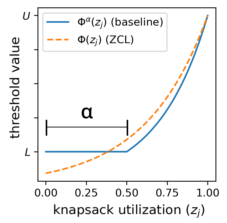
(a)

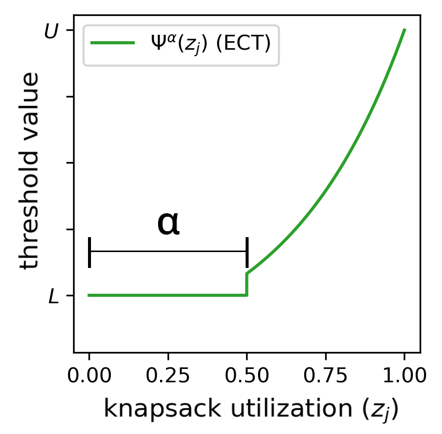
(b)

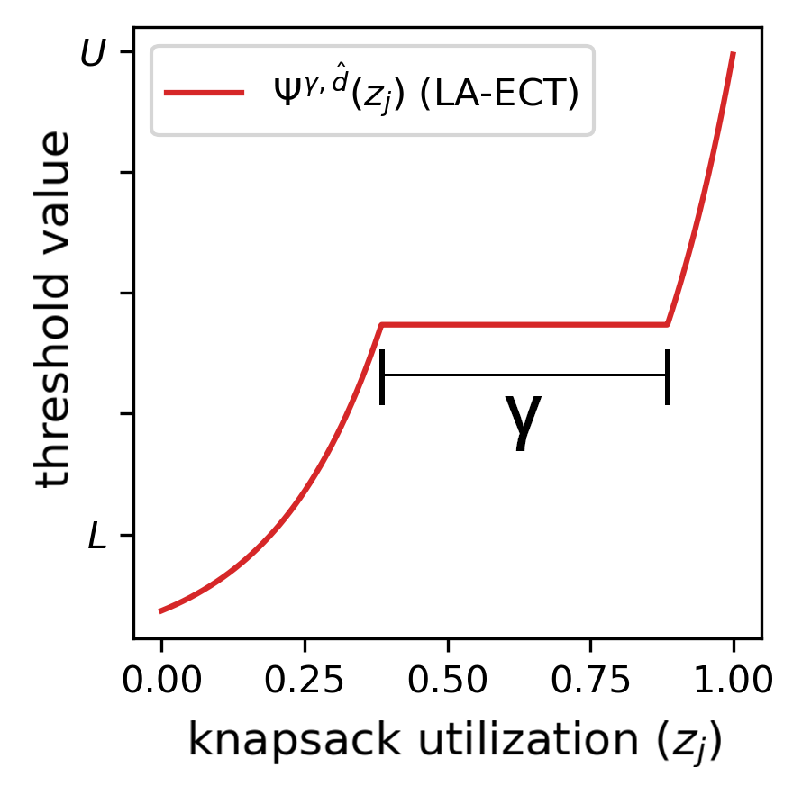
(c)

Figure 1: Plotting the threshold functions for several $\mathsf{OKP}$ algorithms. (a) $\mathsf{ZCL}$ (§3) and the baseline algorithm (see §4); (b) $\mathsf{ECT}$ (§5.1); (c) $\mathsf{LA\text{-}ECT}$ (§5.3)

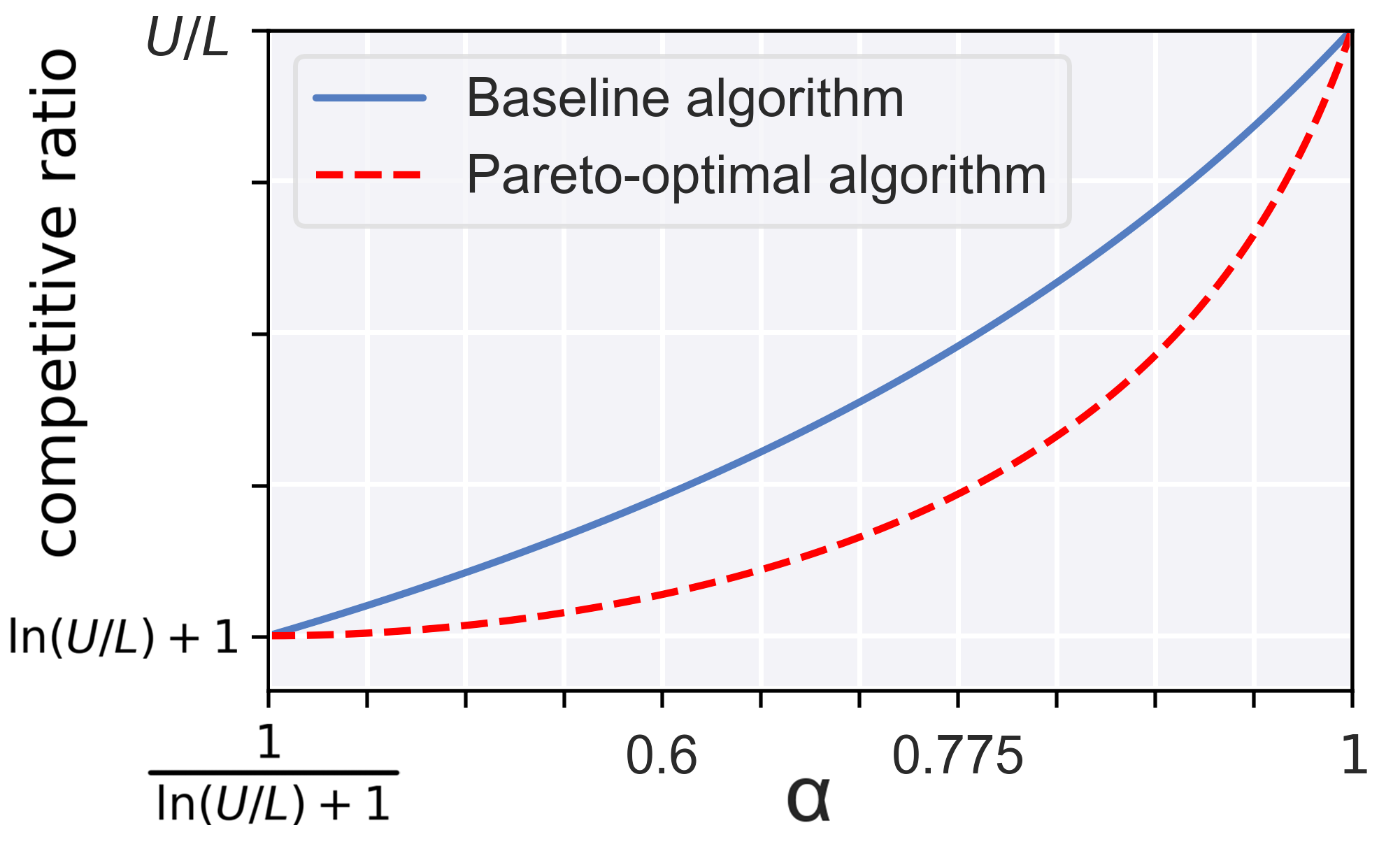
Figure 2: Trade-off for the baseline algorithm and the Pareto-optimal lower bound. $\nicefrac{{U}}{{L}}=5$.

Lower bound. We consider how the $\alpha$-CTIF constraint impacts the achievable competitive ratio for any online deterministic algorithm. To show such a lower bound, we first construct a family of special instances and then show that for any $\alpha$-CTIF online deterministic algorithm (which is not necessarily threshold-based), the competitive ratio is lower bounded under the constructed special instances. It is known that difficult instances for $\mathsf{OKP}$ occur when items arrive at the algorithm in a non-decreasing order of value density [ZCL:08, sun2020competitive]. We now formalize such a family of instances $\{\mathcal{I}_{x}\}_{x\in[L,U]}$, where $\mathcal{I}_{x}$ is called an $x$-continuously non-decreasing instance.

Let $N,m\in\mathbb{N}$ be sufficiently large, and $\delta:=(U-L)/N$. For $x\in[L,U]$, an instance $\mathcal{I}_{x}\in\Omega$ is $x$-continuously non-decreasing if it consists of $N_{x}:=\lceil(x-L)/\delta\rceil+1$ batches of items and the $i$-th batch ($i\in[N_{x}]$) contains $m$ identical items with value density $L+(i-1)\delta$ and weight ${1}/{m}$. Note that $\mathcal{I}_{L}$ is simply a stream of $m$ items, each with weight $\nicefrac{{1}}{{m}}$ and value density $L$. See Fig. 3 for an illustration of an $x$-continuously non-decreasing instance.

No $\alpha$-CTIF deterministic online algorithm for $\mathsf{OKP}$ can achieve a competitive ratio smaller than $\frac{W\left(\frac{U(1-\alpha)}{L\alpha}\right)}{1-\alpha}$, where $W(\cdot)$ is the Lambert $W$ function. Consider the “fair” utilization region of length $\alpha$ for any $\alpha$-CTIF algorithm, and consider the lowest value density $v$ that it accepts in this interval. We show (Lemma 5.1) that it is sufficient to focus on $v=L$ since the competitive ratio is strictly worst if $v>L$. Under an instance $\mathcal{I}_{x}$ (for which the offline optimum is $x$), any $\beta^{\prime}$-competitive deterministic algorithm obtains a value of $\alpha L+\int_{\alpha\beta^{\prime}L}^{x}udg(u)$, where the integrand represents the approximate value obtained from items with value density $u$ and weight allocation $dg(u)$. Using Grönwall’s Inequality yields a necessary condition for the competitive ratio $\beta^{\prime}$ to be $\ln(U/\alpha\beta^{\prime}L)/\beta^{\prime}=1-\alpha$, and the result follows.

Proof.

For any $\alpha$-CTIF deterministic online algorithm $\mathsf{ALG}$, there must exist some utilization region $[a,b]$ with $b-a=\alpha$. Any item that arrives in this region is treated fairly, i.e., by definition of CTIF there exists a function $p(x):[L,U]\rightarrow\{0,1\}$ which characterizes the fair decisions of $\mathsf{ALG}$. We define $v=\min\{x\in[L,U]:p(x)=1\}$ (i.e., $v$ is the lowest value density that $\mathsf{ALG}$ is willing to accept during the fair region).

We first state a lemma (proven afterwards), which asserts that the feasible competitive ratio for any $\alpha$-CTIF deterministic online algorithm with $v>L$ is strictly worse than the feasible competitive ratio when $v=L$.

For any $\alpha$-CTIF deterministic online algorithm $\mathsf{ALG}$ for $\mathsf{OKP}$, if the minimum value density $v$ that $\mathsf{ALG}$ accepts during the fair region of the utilization (of length $\alpha$) is $>L$, then it must have a competitive ratio $\beta^{\prime}\geq{W(\frac{U(1-\alpha)}{L\alpha}e^{\frac{1}{\alpha}})}/{(1-\alpha)}-\frac{1}{\alpha}$, where $W(\cdot)$ is the Lambert W function.

By Lemma 5.1, it suffices to consider the algorithms that set $v=L$.

Given $\mathsf{ALG}$, let $g(x):[L,U]\rightarrow[0,1]$ denote the acceptance function of $\mathsf{ALG}$, where $g(x)$ is the final knapsack utilization under the instance $\mathcal{I}_{x}$. Note that for small $\delta$, processing $\mathcal{I}_{x+\delta}$ is equivalent to first processing $\mathcal{I}_{x}$, and then processing $m$ identical items, each with weight $\frac{1}{m}$ and value density $x+\delta$. Since this function is unidirectional (item acceptances are irrevocable) and deterministic, we must have $g(x+\delta)\geq g(x)$, i.e. $g(x)$ is non-decreasing in $[L,U]$. Once a batch of items with maximum value density $U$ arrives, the rest of the capacity should be used, i.e., $g(U)=1$.

For any algorithm with $v=L$, it will admit all items greedily for an $\alpha$ fraction of the knapsack. Therefore, under the instance $\mathcal{I}_{x}$, the online algorithm with acceptance function $g$ obtains a value of $\mathsf{ALG}(\mathcal{I}_{x})=\alpha L+g(r)r+\int_{r}^{x}udg(u)$, where $udg(u)$ is the value obtained by accepting items with value density $u$ and total weight $dg(u)$, and $r$ is defined as the lowest value density that $\mathsf{ALG}$ is willing to accept during the unfair region, i.e., $r=\inf_{x\in(L,U]:g(x)\geq\alpha}x$.

For any $\beta^{\prime}$-competitive algorithm, we must have $r\leq\alpha\beta^{\prime}L$ since otherwise the worst-case ratio is larger than $\beta^{\prime}$ under an instance $\mathcal{I}_{x}$ with $x=\alpha\beta^{\prime}L+\epsilon$, ($\epsilon>0$). To derive a lower bound of the competitive ratio, observe that it suffices WLOG to focus on algorithms with $r=\alpha\beta^{\prime}L$. This is because if a $\beta^{\prime}$-competitive algorithm sets $r<\alpha\beta^{\prime}L$, then an alternative algorithm can postpone the item acceptance to $r=\alpha\beta^{\prime}L$ and maintain $\beta^{\prime}$-competitiveness.

Under the instance $\mathcal{I}_{x}$, the offline optimal solution obtains a total value of $\mathsf{OPT}(\mathcal{I}_{x})=x$. Therefore, any $\beta^{\prime}$-competitive online algorithm must satisfy:

$$\mathsf{ALG}(\mathcal{I}_{x})=g(L)L+\int_{L}^{x}udg(u)=\alpha L+\int_{r}^{x}udg(u)\geq\frac{x}{\beta^{\prime}},\quad\forall x\in[L,U].$$

By integral by parts and Grönwall’s Inequality (Theorem 1, p. 356, in [Mitrinovic:91]), a necessary condition for the competitive constraint above to hold is the following:

$$g(x) \geq\frac{1}{\beta^{\prime}}-\frac{\alpha L-g(r)r}{x}+\frac{1}{x}\int_{r}^{x}g(u)du$$ (1)

$$\geq\frac{1}{\beta^{\prime}}-\frac{\alpha L}{r}+g(r)+\frac{1}{\beta^{\prime}}\ln\frac{x}{r}=g(\alpha\beta^{\prime}L)+\frac{1}{\beta^{\prime}}\ln\frac{x}{\alpha\beta^{\prime}L},\quad\forall x\in[L,U].$$ (2)

By combining $g(U)=1$ with equation (2), it follows that any deterministic $\alpha$-CTIF and $\beta^{\prime}$-competitive algorithm must satisfy $1=g(U)\geq g(\alpha\beta^{\prime}L)+\frac{1}{\beta^{\prime}}\ln\frac{x}{\alpha\beta^{\prime}L}\geq\alpha+\frac{1}{\beta^{\prime}}\ln\frac{x}{\alpha\beta^{\prime}L}$. The minimal value for $\beta^{\prime}$ can be achieved when both inequalities are tight, and is the solution to $\ln(\frac{U}{\alpha\beta^{\prime}L})/\beta^{\prime}=1-\alpha$. Thus, $\frac{W\left(\frac{U-U\alpha}{L\alpha}\right)}{1-\alpha}$ is a lower bound of the competitive ratio, where $W(\cdot)$ denotes the Lambert $W$ function. ∎

Proof of Lemma 5.1

We use the same definition of the acceptance function $g(x)$ as that in Theorem 5.1. Based on the choice of $v$ by $\mathsf{ALG}$, we consider the following two cases.

Case I: when $v\geq\frac{U}{1+\alpha\beta^{\prime}}$.

Under the instance $\mathcal{I}_{x}$ with $x\in[L,v)$, the offline optimum is $\mathsf{OPT}(\mathcal{I}_{x})=x$ and $\mathsf{ALG}$ can achieve $\mathsf{ALG}(\mathcal{I}_{x})=Lg(L)+\int_{L}^{x}udg(u)$. Thus, any $\beta^{\prime}$-competitive algorithm must satisfy:

$$\mathsf{ALG}(\mathcal{I}_{x})=Lg(L)+\int_{L}^{x}udg(u)\geq\frac{x}{\beta^{\prime}},\quad x\in[L,v).$$

By integral by parts and Grönwall’s Inequality (Theorem 1, p. 356, in [Mitrinovic:91]), a necessary condition for the inequality above to hold is:

$$g(x)\geq\frac{1}{\beta^{\prime}}+\frac{1}{x}\int_{L}^{x}g(u)du\geq\frac{1}{\beta^{\prime}}+\frac{1}{\beta^{\prime}}\ln\frac{x}{L},\forall x\in[L,v).$$

Under the instance $\mathcal{I}_{v}$, to maintain $\alpha$-CTIF , we must have $g(v)\geq\lim_{x\to v}[\frac{1}{\beta^{\prime}}+\frac{1}{\beta^{\prime}}\ln\frac{x}{L}]+\alpha=\frac{1}{\beta^{\prime}}+\frac{1}{\beta^{\prime}}\ln\frac{v}{L}+\alpha$. Thus, we have $1\geq g(v)\geq\frac{1}{\beta^{\prime}}+\frac{1}{\beta^{\prime}}\ln\frac{v}{L}+\alpha$, which gives:

$$\beta^{\prime}\geq\frac{1+\ln\frac{v}{L}}{1-\alpha}.$$ (3)

This lower bound is achieved when $g(x)=\frac{1}{\beta^{\prime}}+\frac{1}{\beta^{\prime}}\ln\frac{x}{L},x\in[L,v)$ and $g(v)=\frac{1}{\beta^{\prime}}+\frac{1}{\beta^{\prime}}\ln\frac{x}{L}+v$. In addition, the total value of accepted items is $\mathsf{ALG}(\mathcal{I}_{v})=\frac{v}{\beta^{\prime}}+\alpha v$.

Under the instance $\mathcal{I}_{x}$ with $x\in(v,U]$, we observe that the worst-case ratio is:

$$\frac{\mathsf{OPT}(\mathcal{I}_{x})}{\mathsf{ALG}(\mathcal{I}_{x})}\leq\frac{U}{\mathsf{ALG}(\mathcal{I}_{v})}=\beta^{\prime}\frac{U}{v(1+\alpha\beta^{\prime})}\leq\beta^{\prime}.$$

Thus, the lower bound of the competitive ratio is dominated by equation (3), and $\beta^{\prime}\geq\frac{1+\ln\frac{v}{L}}{1-\alpha}\geq\frac{1+\ln\frac{U}{L(1+\alpha\beta^{\prime})}}{1-\alpha}$.

Case II: when $L<v<\frac{U}{1+\alpha\beta^{\prime}}$.

In this case, we have the same results under instances $\mathcal{I}_{x},x\in[L,v]$. In particular, $g(v)=\frac{1}{\beta^{\prime}}+\frac{1}{\beta^{\prime}}\ln\frac{x}{L}+v$ and $\mathsf{ALG}(\mathcal{I}_{v})=\frac{v}{\beta^{\prime}}+\alpha v$.

Under the instance $\mathcal{I}_{x}$ with $x\in(v,U]$, the online algorithm can achieve

$$\mathsf{ALG}(\mathcal{I}_{x})=\mathsf{ALG}(\mathcal{I}_{v})+\int_{r}^{x}udg(u),x\in(v,U],$$ (4)

where $r$ is the lowest value density that $\mathsf{ALG}$ admits outside of the fair region. Using the same argument as that in the proof of Theorem 5.1, WLOG we can consider $r=\beta^{\prime}\cdot{\mathsf{ALG}(\mathcal{I}_{v})}=v(1+\alpha\beta^{\prime}),(r<U)$. By integral by parts and Grönwall’s Inequality, a necessary condition for equation (4) is:

$$g(x) \geq\frac{1}{\beta^{\prime}}-\frac{\mathsf{ALG}(\mathcal{I}_{v})-g(r)r}{x}+\frac{1}{x}\int_{r}^{x}g(u)du$$

$$\geq\frac{1}{\beta^{\prime}}-\frac{\mathsf{ALG}(\mathcal{I}_{v})-g(r)r}{r}+\frac{1}{\beta^{\prime}}\ln\frac{x}{r}$$

$$=g(r)+\frac{1}{\beta^{\prime}}\ln\frac{x}{r}.$$

Combining with $g(U)=1$ and $g(r)\geq g(v)$, we have:

$$1=g(U)\geq g(r)+\frac{1}{\beta^{\prime}}\ln\frac{U}{r}\geq\alpha+\frac{1}{\beta^{\prime}}+\frac{1}{\beta^{\prime}}\ln\frac{v}{L}+\frac{1}{\beta^{\prime}}\ln\frac{U}{v(1+\alpha\beta^{\prime})},$$

and thus, the competitive ratio must satisfy:

$$\beta^{\prime}\geq\frac{1+\ln\frac{U}{L(1+\alpha\beta^{\prime})}}{1-\alpha}.$$ (5)

Recall that under the instance $\mathcal{I}_{x}$ with $x\in[L,v)$, the worst-case ratio is:

$$\frac{\mathsf{OPT}(\mathcal{I}_{x})}{\mathsf{ALG}(\mathcal{I}_{x})}\leq\frac{1+\ln\frac{v}{L}}{1-\alpha}<\frac{1+\ln\frac{U}{L(1+\alpha\beta^{\prime})}}{1-\alpha}.$$

Therefore, the lower bound is dominated by equation (5).

Summarizing above two cases, for any $\alpha$-CTIF deterministic online algorithm, if the minimum value density $v$ that it is willing to accept during the fair region is $>L$, then its competitive ratio must satisfy $\beta^{\prime}\geq\frac{1+\ln\frac{U}{L(1+\alpha\beta^{\prime})}}{1-\alpha}$, and the lower bound of the competitive ratio is $\frac{W\left(\frac{(1-\alpha)U}{L\alpha}e^{1/\alpha}\right)}{1-\alpha}$. It is also easy to verify that $\frac{W\left(\frac{(1-\alpha)U}{L\alpha}e^{1/\alpha}\right)}{1-\alpha}\geq\frac{W\left(\frac{U-U\alpha}{L\alpha}\right)}{1-\alpha},\forall\;\alpha\in[\frac{1}{\ln(U/L)+1},1]$. Thus, for any $\alpha$-CTIF algorithm, we focus on the algorithms where $v=L$ in order to minimize the competitive ratio. ∎

Motivated by this Pareto-optimal trade-off, in the following, we design an improved algorithm that closes the theoretical gap between the intuitive baseline algorithm and the lower bound by developing a new threshold function utilizing a discontinuity to be more selective outside the fair region.

Extended Constant Threshold ($\mathsf{ECT}$) for $\mathsf{OKP}$. Let $\alpha\in[\nicefrac{{1}}{{\ln(U/L)+1}},1]$ be a fairness parameter. Given this $\alpha$, we define a threshold function $\Psi^{\alpha}(z)$ on the interval $z\in[0,1]$, where $z$ is the current knapsack utilization. $\Psi^{\alpha}$ is defined as follows (Fig. 2(b)):

$$\Psi^{\alpha}(z)=\begin{cases}L&z\in[0,\alpha],\\ Ue^{\beta(z-1)}&z\in(\alpha,1],\end{cases}$$ (6)

where $\beta=\frac{W\left(\frac{U(1-\alpha)}{L\alpha}\right)}{1-\alpha}$. Let us call this algorithm $\mathsf{ECT}[\alpha]$. The following result shows the achieved trade-off between fairness and competitiveness in $\mathsf{ECT}[\alpha]$.

For any $\alpha\in\left[\nicefrac{{1}}{{\ln(\nicefrac{{U}}{{L}})+1}},1\right]$, $\mathsf{ECT}[\alpha]$ is $\beta$-competitive and $\alpha$-CTIF. For an instance $\mathcal{I}\in\Omega$, suppose $\mathsf{ECT}[\alpha]$ terminates with the utilization at $z_{T}$, and let $W$ and $V$ denote the total weight and total value of the common items picked by $\mathsf{ECT}[\alpha](\mathcal{I})$ and $\mathsf{OPT}(\mathcal{I})$ respectively. Using $\mathsf{OPT}(\mathcal{I})\leq V+\Psi^{\alpha}(z_{T})(1-W)$, we can bound the ratio $\mathsf{OPT}(\mathcal{I})/\mathsf{ECT}[\alpha](\mathcal{I})$ by $\Psi^{\alpha}(z_{T})/\sum_{j\in\mathcal{P}}\Psi^{\alpha}(z_{j})w_{j}$, where $\mathcal{P}$ is the set of items picked by $\mathsf{ECT}[\alpha]$. Taking item weights to be very small, we can approximate this denominator by $\int_{0}^{z_{T}}\Psi^{\alpha}(z)dz$. This quantity can be lower bounded by $L\alpha$ when $z_{T}=\alpha$, and by $\Psi^{\alpha}(z_{T})/\beta$ when $z_{T}>\alpha$, using some careful case analysis. In either case, we can bound the competitive ratio by $\beta$. The $\alpha$-CTIF result is by definition.

Proof.

Fix an arbitrary instance $\mathcal{I}\in\Omega$. When $\mathsf{ECT}[\alpha]$ terminates, suppose the utilization of the knapsack is $z_{T}$, and assume we obtain a value of $\mathsf{ECT}[\alpha](\mathcal{I})$. Let $\mathcal{P}$ and $\mathcal{P}^{\star}$ respectively be the sets of items picked by $\mathsf{ECT}[\alpha]$ and the optimal solution.

Denote the weight and the value of the common items (i.e., the items picked by both $\mathsf{ECT}$ and $\mathsf{OPT}$) by $W=w(\mathcal{P}\cap\mathcal{P}^{\star})$ and $V=v(\mathcal{P}\cap\mathcal{P}^{\star})$. For each item $j$ which is not accepted by $\mathsf{ECT}[\alpha]$, we know that its value density is $<\Psi^{\alpha}(z_{j})\leq\Psi^{\alpha}(z_{T})$ since $\Psi^{\alpha}$ is a non-decreasing function of $z$. Thus,

$$\mathsf{OPT}(\mathcal{I})\leq V+\Psi^{\alpha}(z_{T})(1-W).$$

Since $\mathsf{ECT}[\alpha](\mathcal{I})=V+v(\mathcal{P}\setminus\mathcal{P}^{\star})$, the above inequality implies that

$$\frac{\mathsf{OPT}(\mathcal{I})}{\mathsf{ECT}[\alpha](\mathcal{I})}\leq\frac{V+\Psi^{\alpha}(z_{T})(1-W)}{V+v(\mathcal{P}\setminus\mathcal{P}^{\star})}.$$

Note that, by definition of the algorithm, each item $j$ picked in $\mathcal{P}$ must have value density at least $\Psi^{\alpha}(z_{j})$, where $z_{j}$ is the knapsack utilization when that item arrives. Thus, we have:

$$V\quad \geq\sum_{j\in\mathcal{P}\cap\mathcal{P}^{\star}}\Psi^{\alpha}(z_{j})\;w_{j}=:V_{1},$$

$$v(\mathcal{P}\setminus\mathcal{P}^{\star})\quad \geq\sum_{j\in\mathcal{P}\setminus\mathcal{P}^{\star}}\Psi^{\alpha}(z_{j})\;w_{j}=:V_{2}.$$

Since $\mathsf{OPT}(\mathcal{I})\geq\mathsf{ECT}[\alpha](\mathcal{I})$, we have:

$$\frac{\mathsf{OPT}(\mathcal{I})}{\mathsf{ECT}[\alpha](\mathcal{I})}\leq\frac{V+\Psi^{\alpha}(z_{T})(1-W)}{V+v(\mathcal{P}\setminus\mathcal{P}^{\star})}\leq\frac{V_{1}+\Psi^{\alpha}(z_{T})(1-W)}{V_{1}+v(\mathcal{P}\setminus\mathcal{P}^{\star})}\leq\frac{V_{1}+\Psi^{\alpha}(z_{T})(1-W)}{V_{1}+V_{2}},$$

where the second inequality follows because $\Psi^{\alpha}(z_{T})(1-W)\geq v(\mathcal{P}\setminus\mathcal{P}^{\star})$ and $V_{1}\leq V$.

Note that $V_{1}\leq\Psi^{\alpha}(z_{T})w(\mathcal{P}\cap\mathcal{P}^{\star})=\Psi^{\alpha}(z_{T})W$, and by plugging in for the actual values of $V_{1}$ and $V_{2}$ we get:

$$\frac{\mathsf{OPT}(\mathcal{I})}{\mathsf{ECT}[\alpha](\mathcal{I})}\leq\frac{\Psi^{\alpha}(z_{T})}{\sum_{j\in\mathcal{P}}\Psi^{\alpha}(z_{j})\;w_{j}}.$$

Based on the assumption that individual item weights are much smaller than $1$, we can substitute for $w_{j}$ with $\delta z_{j}=z_{j+1}-z_{j}$ for all $j$. This substitution gives an approximate value of the summation via integration:

$$\sum_{j\in\mathcal{P}}\Psi^{\alpha}(z_{j})\;w_{j} \approx\int_{0}^{z_{T}}\Psi^{\alpha}(z)dz$$

Now there are two cases to analyze – the case where $z_{T}=\alpha$, and the case where $z_{T}>\alpha$. Note that $z_{T}<\alpha$ is impossible, as this means $\mathsf{ECT}[\alpha]$ rejected some item that it had capacity for even when the threshold was at $L$, which is a contradiction. We explore each of the two cases in turn below.

Case I.

If $z_{T}=\alpha$, then $\sum_{j\in\mathcal{P}}\Psi^{\alpha}(z_{j})\;w_{j}\geq L\alpha$.
This follows because $\mathsf{ECT}[\alpha]$ is effectively greedy for at least $\alpha$ utilization of the knapsack, and so the admitted items during this portion must have value at least $L\alpha$. Substituting into the original equation gives us the following:

$$\frac{\mathsf{OPT}(\mathcal{I})}{\mathsf{ECT}[\alpha](\mathcal{I})}\leq\frac{\Psi^{\alpha}(z_{T})}{L\alpha}\leq\beta.$$

Case II.

If $z_{T}>\alpha$, then $\sum_{j\in\mathcal{P}}\Psi^{\alpha}(z_{j})\;w_{j}\approx\int_{0}^{\alpha}Ldz+\int_{\alpha}^{z_{T}}\Psi^{\alpha}(z)dz$.
Solving for the integration, we obtain the following:

$$\sum_{j\in\mathcal{P}}\Psi^{\alpha}(z_{j})\;w_{j} \approx\int_{0}^{\alpha}Ldz+\int_{\alpha}^{z_{T}}\Psi^{\alpha}(z)dz$$

$$=L\alpha+\int_{\alpha}^{z_{T}}Ue^{\beta(z-1)}dz\;=\;L\alpha+\left[\frac{Ue^{\beta(z-1)}}{\beta}\right]_{\alpha}^{z_{T}}$$

$$=L\alpha-\frac{Ue^{\beta(\alpha-1)}}{\beta}+\frac{Ue^{\beta(z_{T}-1)}}{\beta}\;=L\alpha-\frac{\Psi^{\alpha}(\alpha)}{\beta}+\frac{\Psi^{\alpha}(z_{T})}{\beta}=\frac{\Psi^{\alpha}(z_{T})}{\beta}.$$

Substituting into the original equation, we can bound the competitive ratio:

$$\frac{\mathsf{OPT}(\mathcal{I})}{\mathsf{ECT}[\alpha](\mathcal{I})}\leq\frac{\Psi^{\alpha}(z_{T})}{\frac{1}{\beta}\Psi^{\alpha}(z_{T})}=\beta,$$

and the result follows.

Furthermore, the value of $\beta$ which solves the equation $x=\frac{Ue^{x(\alpha-1)}}{L\alpha}$ can be shown as $\frac{W\left(\frac{U-U\alpha}{L\alpha}\right)}{1-\alpha}$, which matches the lower bound from Theorem 5.1. ∎

5.2 Randomization helps

In a follow-up to Theorem 5.1, we can ask whether a randomized algorithm for $\mathsf{OKP}$ exhibits similar trade-offs as in the deterministic setting. We refute this, showing that randomization can satisfy $1$-CTIF while simultaneously obtaining the optimal competitive ratio in expectation.

Motivated by related work on randomized $\mathsf{OKP}$ algorithms, as well as by Theorem 5, we highlight one such randomized algorithm and show that it provides the best possible fairness guarantee. In addition to their optimal deterministic $\mathsf{ZCL}$ algorithm, ZCL:08 also show a related randomized algorithm for $\mathsf{OKP}$; we will henceforth refer to this algorithm as $\mathsf{ZCL\text{-}Randomized}$.

$$\underbrace{{\boxed{\vphantom{i}{}^{v_{.}=L/m}_{w_{.}=1/m}}}{},\dots,{\boxed{\vphantom{i}{}^{v_{.}=L/m}_{w_{.}=1/m}}}{}}_{\text{Batch 0 with }m\text{ items}},\;\underbrace{{\boxed{\vphantom{i}{}^{v_{.}=(L+\delta)/m}_{w_{.}=1/m}}}{},\dots,{\boxed{\vphantom{i}{}^{v_{.}=(L+\delta)/m}_{w_{.}=1/m}}}{}}_{\text{Batch 1 with }m\text{ items}},\;\dots\;\underbrace{{\boxed{\vphantom{i}{}^{v_{.}=x/m}_{w_{.}=1/m}}}{},\dots,{\boxed{\vphantom{i}{}^{v_{.}=x/m}_{w_{.}=1/m}}}{}}_{\text{Batch $N_{x}$ with }m\text{ items}}$$

Figure 3: $\mathcal{I}_{x}$ consists of $N_{x}$ batches of items, arriving in increasing order of value density.

$\mathsf{ZCL\text{-}Randomized}$ samples a constant threshold $\phi$ from the continuous distribution $\mathcal{D}$ over the interval $[0,U]$, with probability density function $f(x)=c/x$ for $L\leq x\leq U$, and $f(x)=c/L$ for $0\leq x\leq L$, where $c=1/[\ln(\nicefrac{{U}}{{L}})+1]$. When item $j$ arrives, $\mathsf{ZCL\text{-}Randomized}$ accepts it iff $v_{j}/w_{j}\geq\phi$ and $z_{j}+w_{j}\leq 1$ (i.e., the item’s value density is above the threshold, and there is enough space for it). The following result shows the competitive optimality of $\mathsf{ZCL\text{-}Randomized}$.

[[ZCL:08], Thms. 3.1, 3.3] $\mathsf{ZCL\text{-}Randomized}$ is $\ln(\nicefrac{{U}}{{L}})+1$-competitive over every input sequence. Furthermore, no online algorithm can achieve a better competitive ratio.

Because $\mathsf{ZCL\text{-}Randomized}$ chooses a random constant threshold before any items arrive, it is trivially $1$-CTIF by Proposition 5. We state this below as a proposition without proof.

$\mathsf{ZCL\text{-}Randomized}$ is $1$-CTIF. Although $\mathsf{ZCL\text{-}Randomized}$ seems to provide the “best of both worlds” from a theoretical perspective, in practice (see §6) we find that it falls short compared to the deterministic algorithms. We believe this is consistent with what has been observed in algorithms for caching [Reineke:14], where randomized techniques are theoretically superior but not used in practice. Motivated by these findings and our deterministic lower bounds, in the next section we draw inspiration from the emerging field of learning-augmented algorithms.

5.3 Prediction helps

In this section, we explore how predictions might help to achieve a better trade-off between competitiveness and fairness. We propose an algorithm, $\mathsf{LA\text{-}ECT}$, which integrates black-box predictions to enhance fairness and competitiveness. We first introduce and formalize our prediction model.

Prediction model. Consider a $1$-CTIF constant threshold algorithm as highlighted in Proposition 5. Although Proposition 5 indicates that any such algorithm with threshold $\phi>L$ cannot have a non-trivial competitive ratio, we know intuitively that increasing $\phi$ makes the algorithm more selective and more competitive. The question, then, is what constant threshold minimizes the competitive ratio on a typical instance? We posit that simple predictions can have a big impact. To motivate the model, we first define an optimal threshold $d^{\star}\in[L,U]$, as follows.

[Optimal threshold $d^{\star}$] Consider an offline approximation algorithm $\mathsf{APX}$ for $\mathsf{OKP}$. Given any $\mathcal{I}\in\Omega$, $\mathsf{APX}(\mathcal{I})$ sorts the items by non-increasing value density and accepts them greedily in this order. If all items are of weight at most $\epsilon$, $\mathsf{APX}(\mathcal{I})$ fills at least $(1-\epsilon)$ portion of the knapsack with the highest value density items, and so $\mathsf{APX}$ has an approximation factor of $1/(1-\epsilon)$. Let $x\in[L,U]$ and $V$ denote the lowest value density of any item and the total value obtained by $\mathsf{APX}(\mathcal{I})$. Then, if the total value of items with value density $x$ chosen in $\mathsf{APX}(\mathcal{I})$ is $\geq V/2$, define $d^{\star}:=x$. Otherwise, define $d^{\star}:=x^{+}$, where $x^{+}$ is the smallest value density in $\mathcal{I}$ larger than $x$. Since $d^{\star}$ is unknown to the online algorithm, we propose a prediction model such that an algorithm receives a single prediction $\hat{d}\in[L,U]$ for each $\mathcal{I}$, where the prediction is perfect if $\hat{d}=d^{\star}$ for $\mathcal{I}$. With this prediction model, we present an online algorithm that incorporates the prediction into its threshold function. We follow the emerging literature on learning-augmented algorithms, where it is standard to evaluate an algorithm based on its consistency and robustness [Lykouris:18, Purohit:18]. Consistency is defined as the competitive ratio of the algorithm when predictions are accurate, while robustness is the worst-case competitive ratio over any prediction errors. These two metrics quantify the power of an algorithm to exploit accurate predictions and ensure bounded competitiveness with poor predictions.

Learning-Augmented Extended Constant Threshold ($\mathsf{LA\text{-}ECT}$) for $\mathsf{OKP}$. Fix two parameters $\gamma\in[0,1]$ and $\hat{d}$, where $\gamma$ is the trust parameter ($\gamma=0$ and $\gamma=1$ correspond to untrusted and fully trusted predictions respectively), and $\hat{d}$ is the prediction. We define a threshold function $\Psi^{\gamma,\hat{d}}(z)$ on the utilization interval $z\in[0,1]$ as follows (see Fig. 2(c)):

$$\Psi^{\gamma,\hat{d}}(z)=\begin{cases}\left(Ue/L\right)^{\frac{z}{1-\gamma}}\left(L/e\right)&z\in[0,\kappa],\\ \hat{d}&z\in(\kappa,\kappa+\gamma),\\ \left(Ue/L\right)^{\frac{z-\gamma}{1-\gamma}}\left(L/e\right)&z\in[\kappa+\gamma,1],\end{cases}$$ (7)

where $\kappa\in[0,1]$ is the point where $(Ue/L)^{(z/1-\gamma)}(L/e)=\hat{d}$. Call the resulting threshold-based algorithm $\mathsf{LA\text{-}ECT}[\gamma]$. The following results characterize the fairness of this algorithm, followed by the results for consistency and robustness, respectively. We omit the proof for Proposition 5.3.

$\mathsf{LA\text{-}ECT}[\gamma]$ is $\gamma$-CTIF.

For any $\mathcal{I}\in\Omega$, let $d_{\max}$ be the highest value density of any item in $\mathcal{I}$, and define $\varrho:=d_{\max}/d^{\star}\geq 1$. Then, for any $\gamma\in(0,1]$, $\mathsf{LA\text{-}ECT}[\gamma]$ is $\frac{\varrho+2}{\gamma}$-consistent for accurate predictions. Assuming the predictions are accurate, the competitive ratio of the algorithm can be analyzed against a semi-online algorithm called $\mathsf{ORACLE}^{\star}$ (Lemma 5.3), which we show to be within a constant factor of $\mathsf{OPT}$. The idea is, for a given arbitrary instance $\mathcal{I}$, to compare the utilization and the total value attained for $\mathcal{I}$ between $\mathsf{ORACLE}^{\star}$ and $\mathsf{LA\text{-}ECT}[\gamma]$ carefully. If our algorithm terminates within the fair region, we can show that it accepts a superset of what $\mathsf{ORACLE}^{\star}$ obtains. If our algorithm terminates after the fair region, we can approximate the total value by means of an integral once again, and carry out a similar case analysis as in Theorems 5.1 or 5.1.

Proof.

For consistency, assume that the prediction $\hat{d}$ is accurate (i.e. $\hat{d}=d^{\star}$). We first consider how well any algorithm can compete against $\mathsf{OPT}$, given that it knows $d^{\star}$ exactly.

In Lemma 5.3, we describe $\mathsf{ORACLE}^{\star}$, a competitive semi-online algorithm [Seiden:00:SemiOnline, Tan:07:SemiOnline, Kumar:19:SemiOnline, Dwibedy:22:SemiOnline]. In other words, it is an algorithm that has full knowledge of the items in the instance, but must process items sequentially using a threshold it has to set in advance. Items still arrive in an online manner, decisions are immediate and irrevocable, and the order of arrival is unknown.

There is a deterministic semi-online algorithm, $\mathsf{ORACLE}^{\star}$, which is $1$-CTIF, and has an approximation factor of $2/(1-\epsilon)$, where $\epsilon$ is the upper bound for item weights. Moreover, no deterministic semi-online algorithm with an approximation factor less than $2-L/U$ is $1$-CTIF.

Proof of Lemma 5.3

Upper bound: Recall the definitions of the offline approximation algorithm $\mathsf{APX}$ and optimal threshold $d^{\star}$ from Definition 5.3. For an arbitrary instance $\mathcal{I}$, let $V$ denote the value obtained by $\mathsf{APX}(\mathcal{I})$, and let $x\in[L,U]$ denote the lowest value density of any item chosen in $\mathsf{APX}(\mathcal{I})$.

Note that $\mathsf{ORACLE}^{\star}$ can compute $d^{\star}$ before the items start coming in. So now suppose $\mathsf{ORACLE}^{\star}$ sets its threshold at $d^{\star}$, and therefore admits any items with value density above $d^{\star}$.

There are two cases, listed below. In each case, we show that $\mathsf{ORACLE}^{\star}$ obtains a value of at least $V/2$:

• If $d^{\star}=x$, we know that the total value of items with value density equal to $x$ in the knapsack of $\mathsf{APX}(\mathcal{I})$ is $V/2$ or larger. Thus, $\mathsf{ORACLE}^{\star}(\mathcal{I})$ accepts items with value density at least $x$, and the total value of items in the knapsack of $\mathsf{ORACLE}^{\star}$ will be $V/2$ or larger.

• Otherwise, if $d^{\star}=x^{+}$ (where $x^{+}$ is strictly larger than $x$ and strictly smaller than the next density in the sorted order), we know that the total value of items with value density $x$ in the knapsack of $\mathsf{APX}$ is less than $V/2$. Thus, $\mathsf{ORACLE}^{\star}(\mathcal{I})$ will reject items of value density $x$, and accept anything with value density larger than $x$, thus obtaining a solution of value at least $V/2$.

Therefore, $\mathsf{ORACLE}^{\star}$ admits a value of at least $V/2$, and its approximation factor is at most $2/(1-\epsilon)$.

Lower bound: Consider an input formed by a large number of infinitesimal items of density $L$ and total weight 1, followed by infinitesimal items of density $U$ and total weight $L/U$. An optimal algorithm accepts all items of density $U$ and fills the remaining space with items of density $L$, giving its knapsack a total value of $(L/U)U+(1-L/U)L=2L-L^{2}/U$. Any deterministic algorithm that satisfies $1$-CTIF, however, must accept either all items of density $L$, giving its knapsack a value of $L$, or reject all items of density $L$, giving it a value of $(L/U)U=L$. In both cases, the approximation factor of the algorithm would be $\frac{2L-L^{2}/U}{L}=2-L/U$. ∎

Using $\mathsf{ORACLE}^{\star}$ as a benchmark, we continue with the proof of Theorem 5.3. Fix an arbitrary input $\mathcal{I}\in\Omega$. Let $\mathsf{LA\text{-}ECT}[\gamma]$ terminate filling $z_{T}$ fraction of the knapsack and obtaining a value of $\mathsf{LA\text{-}ECT}[\gamma](\mathcal{I})$. Let $\mathsf{ORACLE}^{\star}$ terminate filling $z_{O}$ fraction of the knapsack and obtaining a value of $\mathsf{ORACLE}^{\star}(\mathcal{I})$. Denote the maximum possible (offline) value as $\mathsf{OPT}(\mathcal{I})$.

We know that $z_{T}\geq\kappa$, because $\hat{d}$ is an accurate prediction and thus there exist sufficiently many items in the sequence with value density $\geq\hat{d}$. Now we consider two cases – the case where $z_{T}<\kappa+\gamma$, and the case where $z_{T}\geq\kappa+\gamma$. We explore each below.

Case I.

If $z_{T}<\kappa+\gamma$, the following statements must be true:

• $\mathsf{ORACLE}^{\star}(\mathcal{I})$ does not fill the knapsack. If it did, $\mathsf{LA\text{-}ECT}[\gamma](\mathcal{I})$ would be able to accept additional items such that $z_{T}\geq\kappa+\gamma$.

• It must be the case that $z_{O}\leq z_{T}$. Otherwise, since the threshold function $\Psi^{\gamma,\hat{d}}(z)\leq\hat{d}\forall z\leq\kappa+\gamma$, $\mathsf{LA\text{-}ECT}[\gamma](\mathcal{I})$ should have accepted more items such that $z_{T}\geq z_{O}$.

• if $z_{O}=z_{T}$, $\mathsf{ORACLE}^{\star}(\mathcal{I})=\mathsf{LA\text{-}ECT}[\gamma](\mathcal{I})$, and both algorithms admit the same set of items. By definition, any item accepted by $\mathsf{ORACLE}^{\star}(\mathcal{I})$ is accepted by $\mathsf{LA\text{-}ECT}[\gamma](\mathcal{I})$. If any items are accepted by $\mathsf{LA\text{-}ECT}[\gamma](\mathcal{I})$ which are not accepted by $\mathsf{ORACLE}^{\star}(\mathcal{I})$, then it must be the case that $z_{T}>z_{O}$.

• Furthermore, if $z_{O}<z_{T}$, $\mathsf{ORACLE}^{\star}(\mathcal{I})<\mathsf{LA\text{-}ECT}[\gamma](\mathcal{I})$. Again, any item accepted by $\mathsf{ORACLE}^{\star}(\mathcal{I})$ is accepted by $\mathsf{LA\text{-}ECT}[\gamma](\mathcal{I})$, and both knapsacks are not full. Thus, any additional items accepted by $\mathsf{LA\text{-}ECT}[\gamma](\mathcal{I})$ add to the total value achieved by $\mathsf{ORACLE}^{\star}(\mathcal{I})$.

Note that Case I implies that as $\gamma$ approaches $1$, the value obtained by $\mathsf{LA\text{-}ECT}[\gamma](\mathcal{I})$ is greater than or equal to that obtained by $\mathsf{ORACLE}^{\star}(\mathcal{I})$, and we inherit the competitive bound of $\mathsf{ORACLE}^{\star}(\mathcal{I})$ (i.e., $\frac{\mathsf{OPT}(\mathcal{I})}{\mathsf{LA\text{-}ECT}[\gamma\rightarrow 1](\mathcal{I})}\leq 2/(1-\epsilon)$).

Case II.

If $z_{T}\geq\kappa+\gamma$, we consider two sub-cases based on the definition of $d^{\star}$.

First, we derive the worst-case value obtained by $\mathsf{LA\text{-}ECT}$. Denote the items picked by $\mathsf{LA\text{-}ECT}$ by $\mathcal{P}$. Note that each item $j$ picked in $\mathcal{P}$ must have value density of at least $\Psi^{\gamma,\hat{d}}(z_{j})$, where $z_{j}$ is the knapsack utilization when that item arrives. Thus, we have that:

$$\mathsf{LA\text{-}ECT}[\gamma](\mathcal{I}) \geq\sum_{j\in\mathcal{P}}\Psi^{\gamma,\hat{d}}(z_{j})\;w_{j}.$$ (8)

Based on the assumption that individual item weights are much smaller than $1$, we can substitute for $w_{j}$ with $\delta z_{j}:=z_{j+1}-z_{j}$ for all $j$. This substitution allows us to approximate the summation by an integral. We obtain:

$$\sum_{j\in\mathcal{S}}\Psi^{\gamma,\hat{d}}(z_{j})\;w_{j} \approx\int_{0}^{z_{T}}\Psi^{\gamma,\hat{d}}(z)dz=\int_{0}^{z_{T}-\gamma}\left(\frac{Ue}{L}\right)^{\frac{z}{1-\gamma}}\left(\frac{L}{e}\right)dz+\int_{\kappa}^{\kappa+\gamma}d^{\star}\;dz$$

$$\geq d^{\star}\gamma+\int_{0}^{z_{T}-\gamma}\left(\frac{Ue}{L}\right)^{\frac{z}{1-\gamma}}\left(\frac{L}{e}\right)dz$$

$$\geq d^{\star}\gamma+(1-\gamma)\left(\frac{L}{e}\right)\left[\frac{\left(\frac{Ue}{L}\right)^{\frac{z}{1-\gamma}}}{\ln(Ue/L)}\right]_{0}^{z_{T}-\gamma}=d^{\star}\gamma+(1-\gamma)\frac{\Psi^{\gamma,\hat{d}}(z_{T})}{\ln(Ue/L)}.$$

Let $d_{\max}$ denote the largest value density of any item in the sequence $\mathcal{I}$, and note that $\Psi^{\gamma,\hat{d}}(z_{T})=d_{\max}$ by definition. We now consider two different sub-cases based on the definition of $d^{\star}$ (see Definition 5.3) – the case where $d^{\star}=x$, and the case where $d^{\star}=x^{+}$. We explore each below.

• Sub-case II(a): $d^{\star}=x$, where $x\in[L,U]$ is the lowest value density of any item packed into the knapsack of $\mathsf{APX}(\mathcal{I})$. By definition of $\mathsf{ORACLE}^{\star}$ and $d^{\star}$, an algorithm which accepts all of the items with value density $d^{\star}$ in the sequence will be at most $2/(1-\epsilon)$-competitive against $\mathsf{OPT}(\mathcal{I})$. Thus, since $\mathsf{LA\text{-}ECT}[\gamma](\mathcal{I})\geq d^{\star}\gamma+(1-\gamma)\frac{d_{\max}}{\ln(Ue/L)}$, the following holds:

  $$\frac{\mathsf{OPT}(\mathcal{I})}{\mathsf{LA\text{-}ECT}[\gamma](\mathcal{I})}\leq\frac{\mathsf{OPT}(\mathcal{I})}{d^{\star}\gamma+(1-\gamma)\frac{d_{\max}}{\ln(Ue/L)}}\leq\frac{\mathsf{OPT}(\mathcal{I})}{d^{\star}\gamma}\leq\frac{2/(1-\epsilon)}{\gamma}.$$ (9)

• Sub-case II(b): $d^{\star}=x^{+}$, where $x^{+}\in[L,U]$ denotes the value density marginally higher than $x$ (lowest value density in the knapsack of $\mathsf{APX}(\mathcal{I})$) but lower than the next highest value density in the list of sorted value densities. Since $d_{\max}$ is the highest value density for any item in the instance, it is also the largest value density accepted by $\mathsf{APX}(\mathcal{I})$.

  In the worst-case, items arrive in non-decreasing order of value density, so $\mathsf{LA\text{-}ECT}[\gamma](\mathcal{I})$ fills $\gamma$ fraction of its knapsack with items of value density exactly equal to $d^{\star}$.

  Suppose that the next higher value density is $d_{\max}$. In the worst-case, by definition of $\mathsf{APX}(\mathcal{I})$, the total weight of items with value density $d_{\max}$ is at most $(1-\gamma)$ (otherwise, $\mathsf{LA\text{-}ECT}[\gamma](\mathcal{I})$ will be able to accept some of these higher-valued items in the $\gamma$-CTIF region). $\mathsf{OPT}(\mathcal{I})$ will accept all of the items in the instance with value densities $d_{\max}$, $d^{\star}$, and potentially some items with value densities lower than $d^{\star}$ to fill the rest of the knapsack – in the worst-case, $\mathsf{OPT}(\mathcal{I})\leq d^{\star}\gamma+d_{\max}(1-\gamma)$. Recalling that $\varrho=d_{\max}/d^{\star}$, we have the following:

  $$\frac{\mathsf{OPT}(\mathcal{I})}{\mathsf{LA\text{-}ECT}[\gamma](\mathcal{I})}\leq\frac{d^{\star}\gamma+d_{\max}(1-\gamma)}{d^{\star}\gamma+(1-\gamma)\frac{d_{\max}}{\ln(Ue/L)}}\leq\frac{d^{\star}\gamma+d_{\max}(1-\gamma)}{d^{\star}\gamma}\leq\frac{d_{\max}}{d^{\star}\gamma}=\frac{\varrho}{\gamma}$$ (10)

It follows in either case that $\mathsf{LA\text{-}ECT}[\gamma]$ is $\frac{\varrho+2}{\gamma}$-consistent for accurate predictions.

In practice, it is often reasonable to assume that $\varrho=d_{\max}/d^{\star}$ is relatively small, e.g. $\varrho=O(1)$. Recall that in sub-case II(b), $d_{\max}$ is the largest value density of any item in the sequence and $d^{\star}=x^{+}$. Observe that $d_{\max}$ and $d^{\star}$ correspond to the largest and (nearly) smallest value densities accepted into the knapsack of $\mathsf{APX}(\mathcal{I})$, which sorts items by value density in non-increasing order and accepts them greedily in that order. Thus, if such an assumption holds, $\mathsf{LA\text{-}ECT}[\gamma]$ is at most $O\left(\frac{1}{\gamma}\right)$-consistent for accurate predictions. In §6, our experimental results further support this assumption.

It is important, however, to note that in theory, there are simple, artificial counterexamples where this assumption may not hold. For instance, if the $\varrho\approx\frac{U}{L}$, our assumption no longer holds and the consistency bound is no longer meaningful. Notably, under such a counterexample we know that any nontrivial algorithm achieves good empirical competitiveness, as $d^{\star}\thicksim L$ implies that a knapsack of unit capacity can accept all or nearly all of the items. ∎

Remark .

For most instances, we assume that $\varrho=O(1)$, implying that $d_{\max}=O(d^{\star})$. Whenever this assumption holds, Theorem 5.3 implies that $\mathsf{LA\text{-}ECT}[\gamma]$ is $O(1/\gamma)$-consistent.
In §6, our experimental results further support this assumption as reasonable in practice.

For any $\gamma\in[0,1]$, $\mathsf{LA\text{-}ECT}[\gamma]$ is $\frac{1}{1-\gamma}\left(\ln(\nicefrac{{U}}{{L}})+1\right)$-robust for any $\mathcal{I}\in\Omega$. As in the proof of Theorem 5.1, we can bound $\mathsf{OPT}(\mathcal{I})/\mathsf{LA\text{-}ECT}[\gamma](\mathcal{I})$ for any $\mathcal{I}\in\Omega$ by $\Psi^{\gamma,\hat{d}}(z_{T})/\sum_{j\in\mathcal{P}}\Psi^{\gamma,\hat{d}}(z_{j})w_{j}$, where the notation follows from before. By assuming that the individual weights are much smaller than $1$, we can approximate this denominator by an integral once again, and consider three cases. When $z_{T}<\kappa$, we can bound the integral by $(1-\gamma)\Psi^{\gamma,\hat{d}}(z_{T})/\ln(Ue/L)$, which suffices for our bound. When $\kappa\leq z_{T}<\kappa+\gamma$, we can show an improvement from the previous case, inheriting the same worst-case bound. Finally, when $z_{T}\geq\kappa+\gamma$, we can inherit the same approximation as in the first case with a negligible additive term of $\hat{d}\gamma$. In each case, the bound on the competitive ratio follows in a straightforward way.

Proof.

Fix an arbitrary input sequence $\mathcal{I}$. Let $\mathsf{LA\text{-}ECT}[\gamma]$ terminate filling $z_{T}$ fraction of the knapsack and obtaining a value of $\mathsf{LA\text{-}ECT}[\gamma](\mathcal{I})$. Let $\mathcal{P}$ and $\mathcal{P}^{\star}$ respectively be the sets of items picked by $\mathsf{LA\text{-}ECT}[\gamma]$ and the optimal solution.

Denote the weight and the value of the common items (items picked by both $\mathsf{LA\text{-}ECT}$ and $\mathsf{OPT}$) by $W=w(\mathcal{P}\cap\mathcal{P}^{\star})$ and $V=v(\mathcal{P}\cap\mathcal{P}^{\star})$. For each item $j$ which is not accepted by $\mathsf{LA\text{-}ECT}[\gamma]$, we know that its value density is $<\Psi^{\gamma,\hat{d}}(z_{j})\leq\Psi^{\gamma,\hat{d}}(z_{T})$ since $\Psi^{\gamma,\hat{d}}$ is a non-decreasing function of $z$. Thus, we have:

$$\mathsf{OPT}(\mathcal{I})\leq V+\Psi^{\gamma,\hat{d}}(z_{T})(1-W).$$

Since $\mathsf{LA\text{-}ECT}[\gamma](\mathcal{I})=V+v(\mathcal{P}\setminus\mathcal{P}^{\star})$, the inequality above implies that:

$$\frac{\mathsf{OPT}(\mathcal{I})}{\mathsf{LA\text{-}ECT}[\gamma](\mathcal{I})}\leq\frac{V+\Psi^{\gamma,\hat{d}}(z_{T})(1-W)}{V+v(\mathcal{P}\setminus\mathcal{P}^{\star})}.$$

Note that each item $j$ picked in $\mathcal{P}$ must have value density of at least $\Psi^{\gamma,\hat{d}}(z_{j})$, where $z_{j}$ is the knapsack utilization when that item arrives. Thus, we have that:

$$V\quad \geq\sum_{j\in\mathcal{P}\cap\mathcal{P}^{\star}}\Psi^{\gamma,\hat{d}}(z_{j})\;w_{j}=:V_{1},$$

$$v(\mathcal{P}\setminus\mathcal{P}^{\star})\quad \geq\sum_{j\in\mathcal{P}\setminus\mathcal{P}^{\star}}\Psi^{\gamma,\hat{d}}(z_{j})\;w_{j}=:V_{2}.$$

Since $\mathsf{OPT}(\mathcal{I})\geq\mathsf{LA\text{-}ECT}[\gamma](\mathcal{I})$, we have that

$$\frac{\mathsf{OPT}(\mathcal{I})}{\mathsf{LA\text{-}ECT}[\gamma](\mathcal{I})}\leq\frac{V+\Psi^{\gamma,\hat{d}}(z_{T})(1-W)}{V+v(\mathcal{P}\setminus\mathcal{P}^{\star})}\leq\frac{V_{1}+\Psi^{\gamma,\hat{d}}(z_{T})(1-W)}{V_{1}+V_{2}}.$$

Note that $V_{1}\leq\Psi^{\gamma,\hat{d}}(z_{T})w(\mathcal{P}\cap\mathcal{P}^{\star})=\Psi^{\gamma,\hat{d}}(z_{T})W$, and so, plugging in the actual values of $V_{1}$ and $V_{2}$, we get:

$$\frac{\mathsf{OPT}(\mathcal{I})}{\mathsf{LA\text{-}ECT}[\gamma](\mathcal{I})}\leq\frac{\Psi^{\gamma,\hat{d}}(z_{T})}{\sum_{j\in\mathcal{P}}\Psi^{\gamma,\hat{d}}(z_{j})\;w_{j}}.$$

Based on the assumption that individual item weights are much smaller than $1$, we can substitute for $w_{j}$ with $\delta z_{j}=z_{j+1}-z_{j}$ for all $j$. This substitution allows us to obtain an approximate value of the summation via integration:

$$\sum_{j\in\mathcal{P}}\Psi^{\gamma,\hat{d}}(z_{j})\;w_{j} \approx\int_{0}^{z_{T}}\Psi^{\gamma,\hat{d}}(z)dz$$

Now we consider three separate cases – the case where $z_{T}\in[0,\kappa)$, the case where $z_{T}\in[\kappa,\kappa+\gamma)$, and the case where $z_{T}\in[\kappa+\gamma,1]$. We explore each below.

Case I.

If $z_{T}\in[0,\kappa)$, $\mathsf{OPT}(\mathcal{I})$ is bounded by $\Psi^{\gamma,\hat{d}}(z_{T})\leq\hat{d}$. Furthermore,

$$\sum_{j\in\mathcal{P}}\Psi^{\gamma,\hat{d}}(z_{j})\;w_{j} \approx\int_{0}^{z_{T}}\Psi^{\gamma,\hat{d}}(z)dz\;=\int_{0}^{z_{T}}\left(\frac{Ue}{L}\right)^{\frac{z}{1-\gamma}}\left(\frac{L}{e}\right)dz$$

$$=(1-\gamma)\left(\frac{L}{e}\right)\left[\frac{\left(\frac{Ue}{L}\right)^{\frac{z}{1-\gamma}}}{\ln(Ue/L)}\right]_{0}^{z_{T}}=(1-\gamma)\frac{\Psi^{\gamma,\hat{d}}(z_{T})}{\ln(Ue/L)}$$

Combined with the previous equation for the competitive ratio, this gives us the following:

$$\frac{\mathsf{OPT}(\mathcal{I})}{\mathsf{LA\text{-}ECT}[\gamma](\mathcal{I})}\leq\frac{\Psi^{\gamma,\hat{d}}(z_{T})}{(1-\gamma)\frac{\Psi^{\gamma,\hat{d}}(z_{T})}{\ln(\nicefrac{{U}}{{L}})+1}}\leq\frac{\hat{d}}{(1-\gamma)\frac{\hat{d}}{\ln(\nicefrac{{U}}{{L}})+1}}=\frac{1}{1-\gamma}\left(\ln(\nicefrac{{U}}{{L}})+1\right).$$

Case II.

If $z_{T}\in[\kappa,\kappa+\gamma)$, $\mathsf{OPT}(\mathcal{I})$ is bounded by $\Psi^{\gamma,\hat{d}}(z_{T})=\hat{d}$. Furthermore,

$$\int_{0}^{z_{T}}\Psi^{\gamma,\hat{d}}(z)dz=\int_{0}^{\kappa}\left(\frac{Ue}{L}\right)^{\frac{z}{1-\gamma}}\left(\frac{L}{e}\right)dz+\int_{\kappa}^{z_{T}}\hat{d}\;dz\geq\int_{0}^{\kappa}\left(\frac{Ue}{L}\right)^{\frac{z}{1-\gamma}}\left(\frac{L}{e}\right)dz.$$

Note that since the bound on $\mathsf{OPT}(\mathcal{I})$ can be the same (i.e. $\mathsf{OPT}(\mathcal{I})\leq\hat{d}$), Case I is strictly worse than Case II for the competitive ratio, and we inherit the worse bound:

$$\frac{\mathsf{OPT}(\mathcal{I})}{\mathsf{LA\text{-}ECT}[\gamma](\mathcal{I})}\leq\frac{\hat{d}}{(1-\gamma)\frac{\hat{d}}{\ln(\nicefrac{{U}}{{L}})+1}}=\frac{1}{1-\gamma}\left(\ln(\nicefrac{{U}}{{L}})+1\right).$$

Case III.

If $z_{T}\in[\kappa+\gamma,1]$, $\mathsf{OPT}(\mathcal{I})$ is bounded by $\Psi^{\gamma,\hat{d}}(z_{T})\leq U$. Furthermore,

$$\sum_{j\in\mathcal{P}}\Psi^{\gamma,\hat{d}}(z_{j})\;w_{j} \approx\int_{0}^{z_{T}}\Psi^{\gamma,\hat{d}}(z)dz\;=\int_{0}^{z_{T}-\gamma}\left(\frac{Ue}{L}\right)^{\frac{z}{1-\gamma}}\left(\frac{L}{e}\right)dz+\int_{\kappa}^{\kappa+\gamma}\hat{d}\;dz$$

$$=(1-\gamma)\left(\frac{L}{e}\right)\left[\frac{\left(\frac{Ue}{L}\right)^{\frac{z}{1-\gamma}}}{\ln(Ue/L)}\right]_{0}^{z_{T}-\gamma}+\gamma\hat{d}$$

$$=(1-\gamma)\frac{\Psi^{\gamma,\hat{d}}(z_{T})}{\ln(Ue/L)}+\gamma\hat{d}.$$

Combined with the previous equation for the competitive ratio, this gives us the following:

$$\frac{\mathsf{OPT}(\mathcal{I})}{\mathsf{LA\text{-}ECT}[\gamma](\mathcal{I})}\leq\frac{\Psi^{\gamma,\hat{d}}(z_{T})}{(1-\gamma)\frac{\Psi^{\gamma,\hat{d}}(z_{T})}{\ln(\nicefrac{{U}}{{L}})+1}+\gamma\hat{d}}\leq\frac{\Psi^{\gamma,\hat{d}}(z_{T})}{(1-\gamma)\frac{\Psi^{\gamma,\hat{d}}(z_{T})}{\ln(\nicefrac{{U}}{{L}})+1}}=\frac{1}{1-\gamma}\left(\ln(\nicefrac{{U}}{{L}})+1\right).$$

Since we have shown that $\mathsf{LA\text{-}ECT}[\gamma](\mathcal{I})$ obtains at least $\frac{1}{1-\gamma}\left(\ln(\nicefrac{{U}}{{L}})+1\right)$ of the value obtained by $\mathsf{OPT}(\mathcal{I})$ in each case, we conclude that $\mathsf{LA\text{-}ECT}[\gamma](\mathcal{I})$ is $\frac{1}{1-\gamma}\left(\ln(\nicefrac{{U}}{{L}})+1\right)$-robust. ∎

6 Numerical Experiments

In this section, we present experimental results for $\mathsf{OKP}$ algorithms in the context of the online job scheduling problem from Example 1. We evaluate our proposed algorithms, including $\mathsf{ECT}$ and $\mathsf{LA\text{-}ECT}$, against existing algorithms from the literature.

Setup and data set. To validate the performance of our algorithms and estimate the impact of fairness constraints in an application, we conduct experiments using a real-world data set for online cloud job scheduling. Specifically, we extract item sequences from Google cluster traces [Reiss:12]. We consider a server with a one-dimensional resource (i.e., CPU) and set the capacity to $1$. The resource requirement of each job is uniformly drawn from three possible “weights” $w_{j}\in[0.01,0.03,0.05]$. Each job in the data has a innate value of $\iota_{j}$. The ratio between the maximum and minimum such values is 50. To simulate different value density ratios $\nicefrac{{U}}{{L}}$, we set the value of each job to $v_{j}=\tau_{j}\iota_{j}w_{j}$, where $\tau_{j}$ is a uniform random variable in $[1,\mu]$. We then evaluate the average and worst-case performances of the tested algorithms when $\mu\in\{10,25,50\}$, which correspond to values for $\nicefrac{{U}}{{L}}$ of $500$, $1250$, and $2500$, respectively. We report the cumulative density functions of the empirical competitive ratios, which show the average and the worst-case performances of several algorithms as described below.

Comparison algorithms. As an offline benchmark, we use a dynamic programming approach to calculate the optimal offline solution for each given sequence and objective, which allows us to report the empirical competitive ratio for each tested algorithm. In the setting without predictions, we compare our proposed $\mathsf{ECT}$ algorithm against three other algorithms: $\mathsf{ZCL}$, the baseline $\alpha$-CTIF algorithm, and $\mathsf{ZCL\text{-}Randomized}$ (§3, §5.1, and §5.2 respectively). For $\mathsf{ECT}$, we set several values for $\alpha$ to show how performance degrades with more stringent fairness guarantees.
In the setting with predictions, we compare our proposed $\mathsf{LA\text{-}ECT}$ algorithm (§5.3) against two other algorithms: $\mathsf{ZCL}$ and $\mathsf{ECT}$. Simulated predictions are obtained by first solving for the perfect value $d^{\star}$ (Defn. 5.3). For simulated prediction error, we set $\hat{d}=d^{\star}(1+\eta)$, where $\eta\sim\mathcal{N}(0,\sigma)$. In this setting, we fix a single value for $\nicefrac{{U}}{{L}}$ and report results for different levels of error obtained by changing $\sigma$.

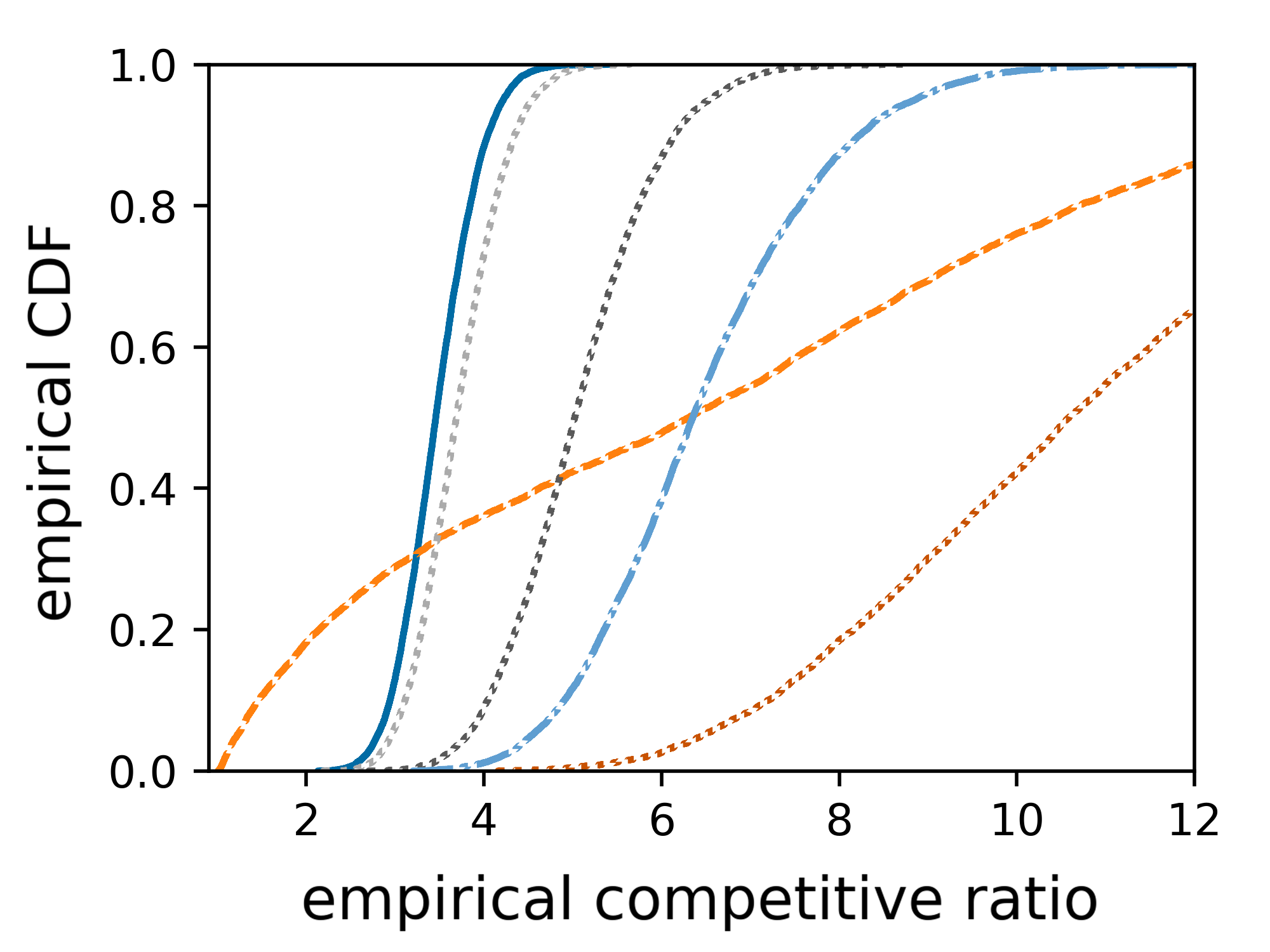
(a) $\nicefrac{{U}}{{L}}=500$

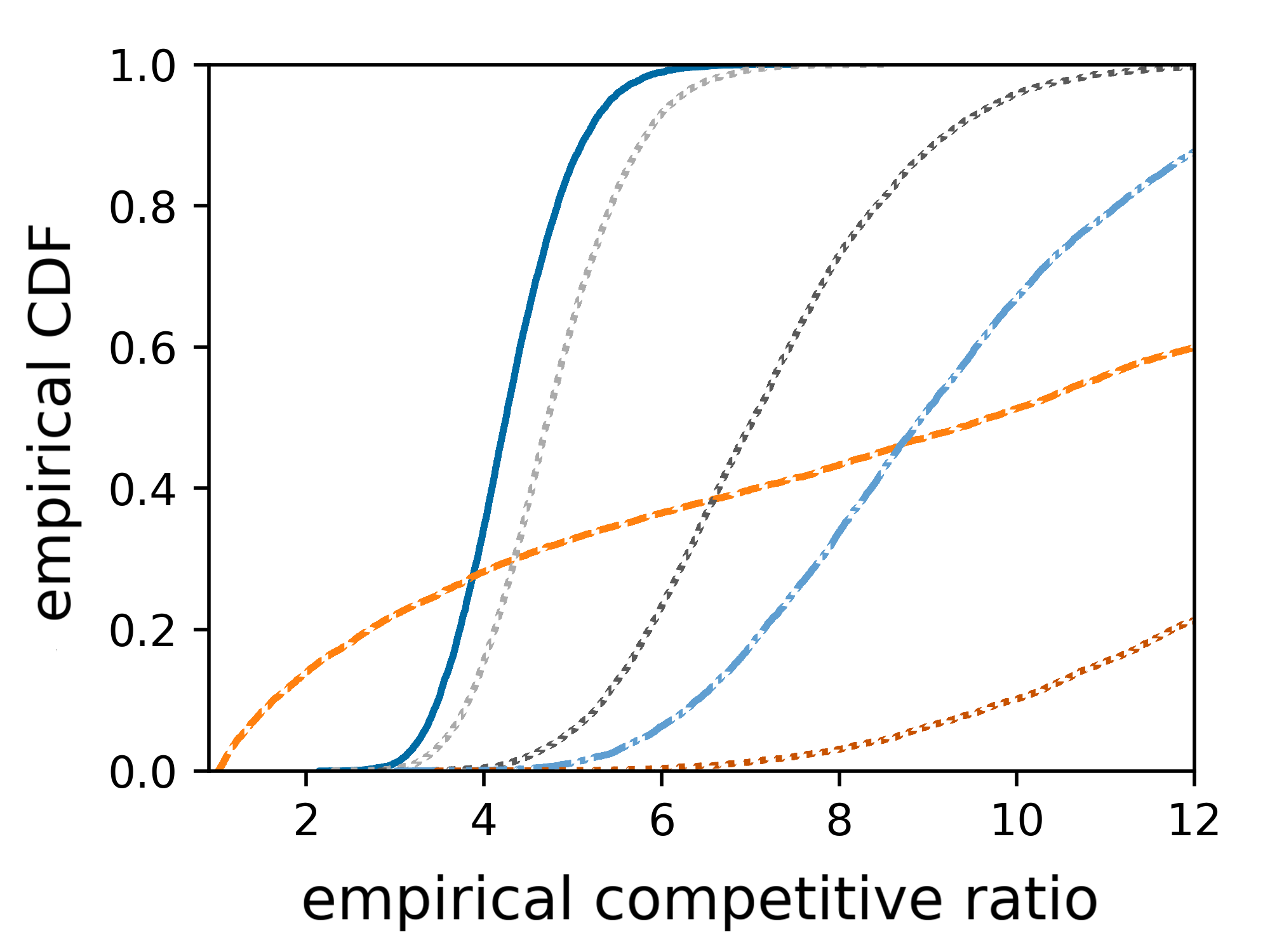
(b) $\nicefrac{{U}}{{L}}=2500$

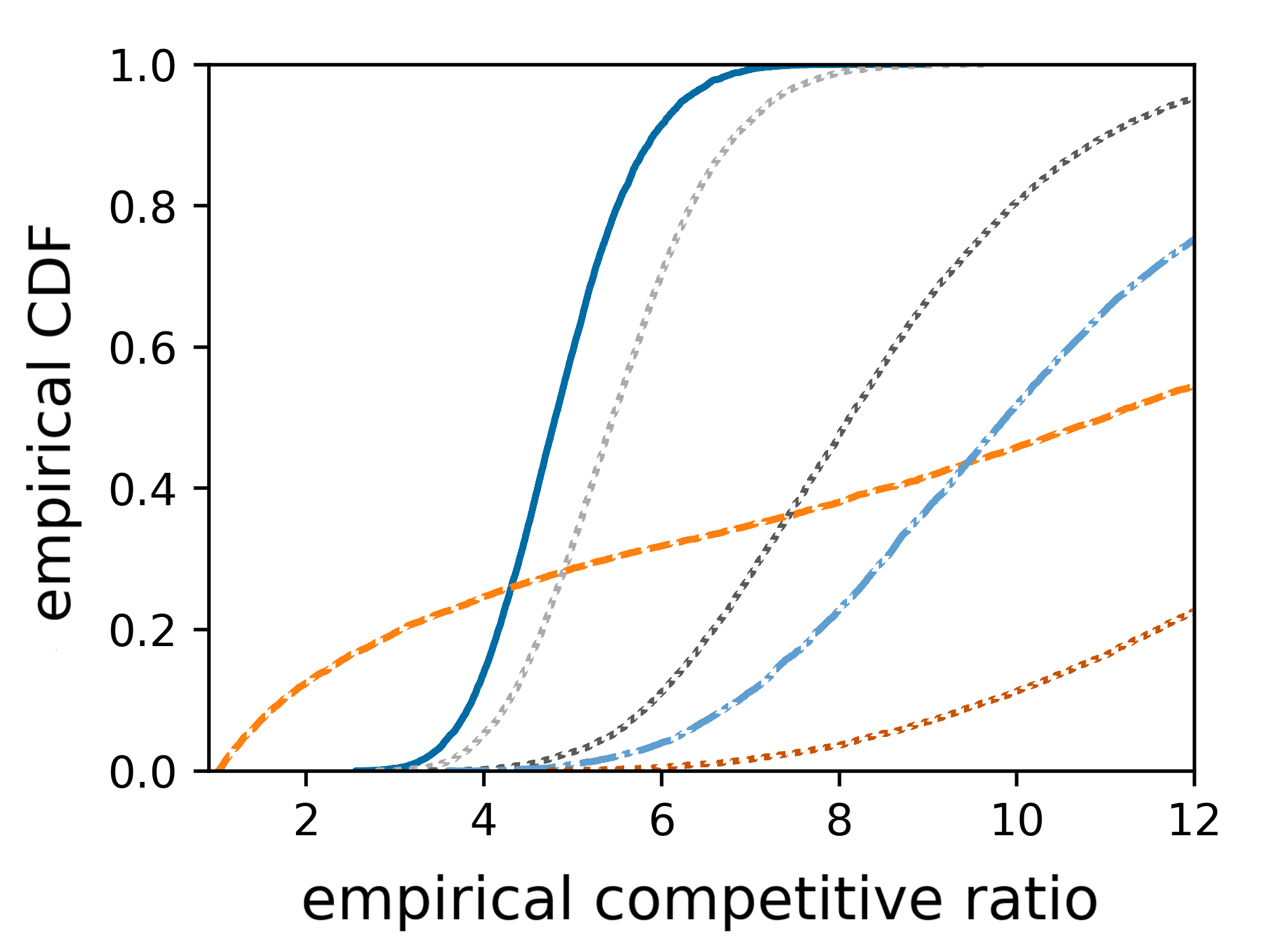
(c) $\nicefrac{{U}}{{L}}=10000$

Figure 4: Cloud scheduling experiments, with varying value density fluctuation $\nicefrac{{U}}{{L}}$.

Experimental results. We report the empirical competitive ratio, and intuitively, we expect worse empirical competitiveness for those algorithms which provide stronger fairness guarantees. In the first experiment, we test the deterministic and randomized algorithms for $\mathsf{OKP}$ in the setting without predictions, for several values of $\nicefrac{{U}}{{L}}$. As $\nicefrac{{U}}{{L}}$ grows, the upper bounds on the competitive ratios of all tested algorithms also grow. In Fig. 4, we show the CDF of the empirical competitive ratios for each tested value of $\nicefrac{{U}}{{L}}$. We observe that the performance of $\mathsf{ECT}[\alpha]$ exactly corresponds with the fairness parameter $\alpha$, meaning that a greater value of $\alpha$ corresponds with a worse competitive ratio, as shown in Theorems 5.1 and 5.1. Reflecting the theoretical results, $\mathsf{ECT}[\alpha]$ outperforms the baseline algorithm for $\alpha=0.66$ by an average of $20.9\%$ across all experiments.
Importantly, we also observe that $\mathsf{ZCL\text{-}Randomized}$ performs poorly compared to the deterministic algorithms. This is an interesting departure from the theory since Theorem 3 and Proposition 5.2 tell us that $\mathsf{ZCL\text{-}Randomized}$ should be optimally competitive and completely fair. We attribute this gap to the “one-shot” randomization used in the design of $\mathsf{ZCL\text{-}Randomized}$ – although picking a single random threshold may yield good performance in expectation, the probability of picking a bad threshold is relatively high. Coupled with the observation that $\mathsf{ZCL}$ and $\mathsf{ECT}$ often significantly outperform their theoretical bounds, this leaves $\mathsf{ZCL\text{-}Randomized}$ at a disadvantage.

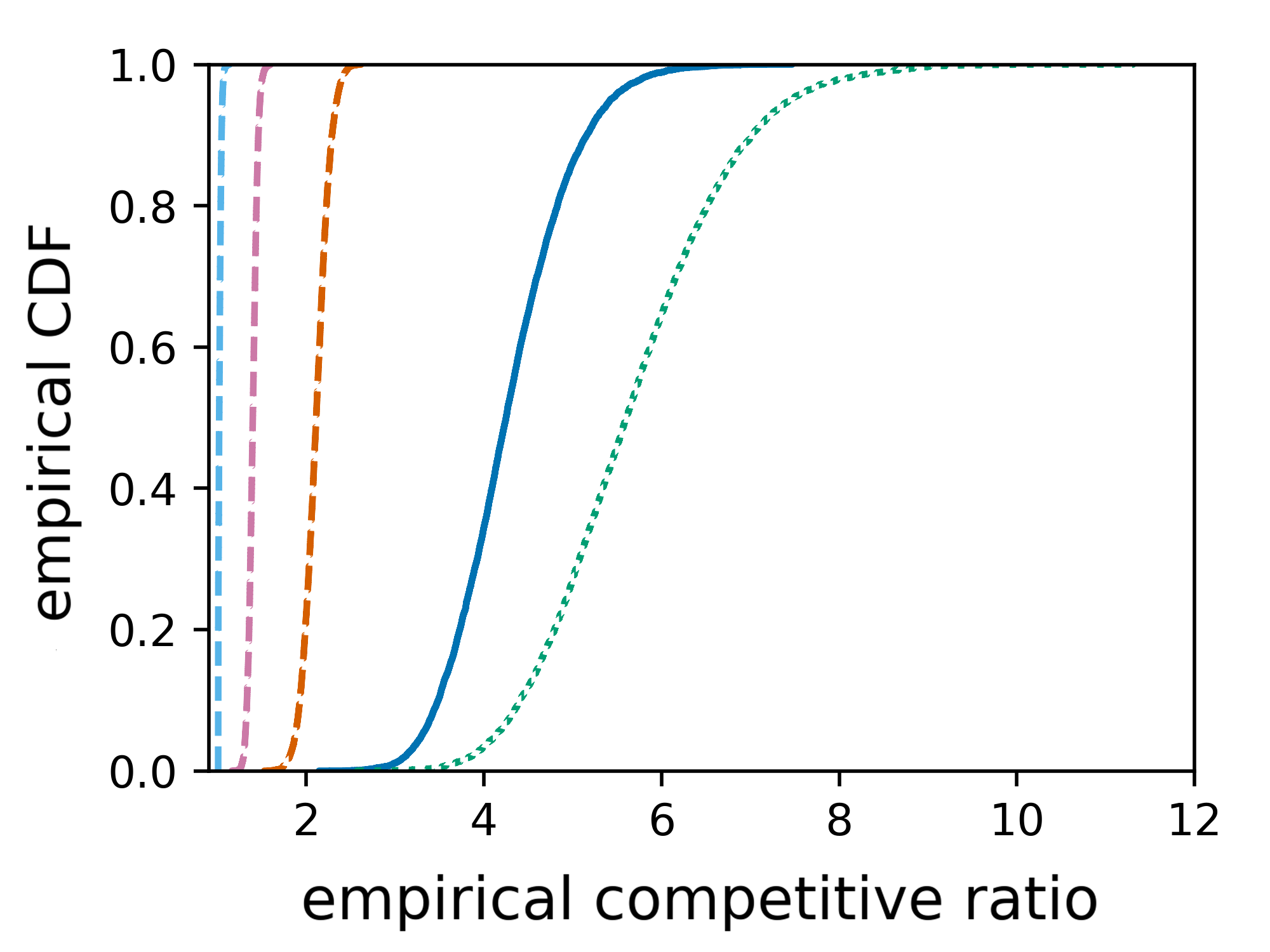
(a) $\sigma=0$ (perfect predictions)

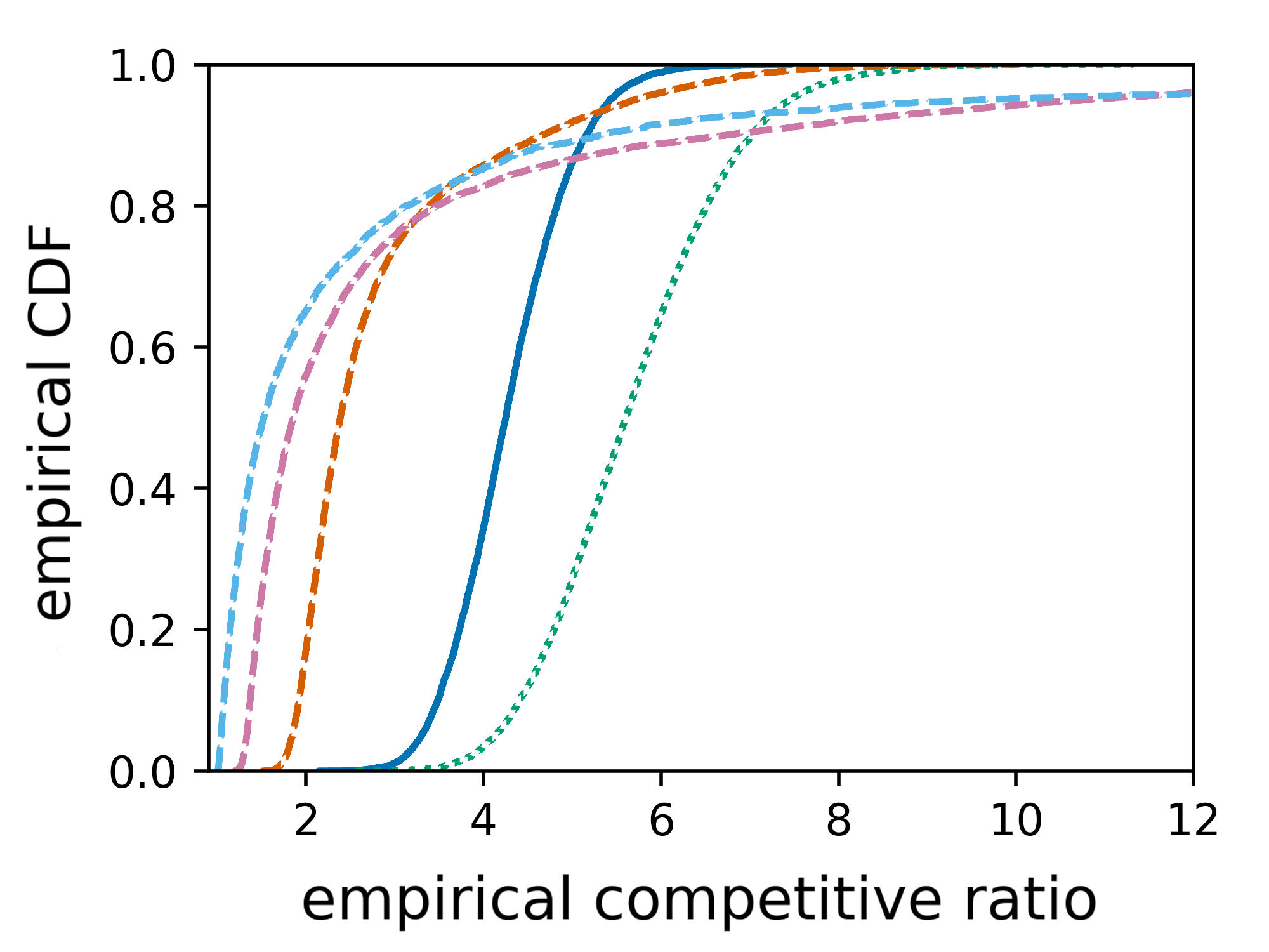
(b) $\sigma=1/2$

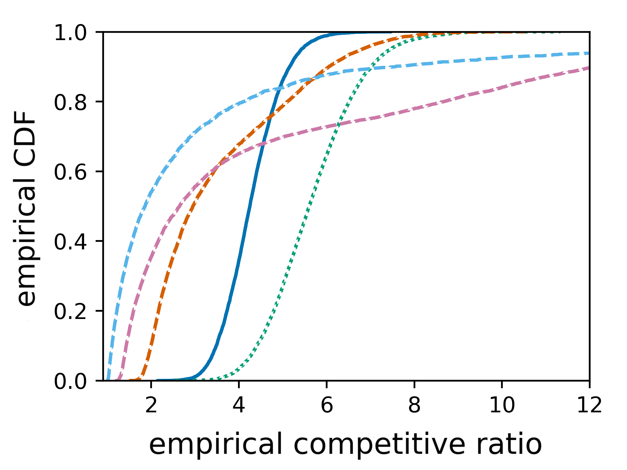
(c) $\sigma=1$

Figure 5: Learning-augmented experiments, with $\nicefrac{{U}}{{L}}=2500$ and different prediction errors.

In the second experiment, we investigate the impact of prediction error in the setting with predictions. We fix $\nicefrac{{U}}{{L}}=2,500$ and vary $\sigma$, which is the standard deviation of the multiplicative error quantity $\eta$. In Fig. 5, we show the CDF of the empirical competitive ratios for each error regime. $\mathsf{LA\text{-}ECT}[\gamma]$ performs very well with perfect predictions (Fig. 5(a)) – with fully trusted predictions, it is nearly $1$-competitive against $\mathsf{OPT}$, and all of the learning-augmented algorithms significantly outperform both $\mathsf{ZCL}$ and $\mathsf{ECT}$. As the prediction error increases (Figs. 5(b) and 5(c)), the tails of the CDFs degrade accordingly. $\mathsf{LA\text{-}ECT}[\gamma=1]$ fully trusts the prediction and there is no robustness guarantee – as such, increasing the prediction error induces an unbounded empirical competitive ratio for this case. For other values of $\gamma$, higher error intuitively has a greater impact when the trust parameter $\gamma$ is larger. Notably, $\mathsf{LA\text{-}ECT}[\gamma=0.33]$ maintains a worst-case competitive ratio roughly on par with $\mathsf{ECT}$ in every error regime while performing better than $\mathsf{ZCL}$ and $\mathsf{ECT}$ on average across the board.

7 Conclusion

We study time fairness in the online knapsack problem ($\mathsf{OKP}$), showing impossibility results for existing notions, and proposing a definition of conditional time-independent fairness, which is generalizable. We give a deterministic algorithm achieving the Pareto-optimal trade-off between fairness and efficiency, and explore the power of randomization and simple predictions. Evaluating our $\mathsf{ECT}$ and $\mathsf{LA\text{-}ECT}$ algorithms in trace-driven experiments, we observe positive results for competitiveness compared to existing algorithms in exchange for significantly improved fairness guarantees.

Limitations and future work.

There are several interesting directions of inquiry that we have not considered which would be good candidates for future work. It would be interesting to apply our notion of time fairness in other online problems such as one-way trading and bin packing, among others [ElYaniv:01, Lorenz:08, Balogh:17:BP, Johnson:74:BP, Ma:21, Balseiro:22]. Another fruitful direction is exploring the notion of group fairness [Patel:20] in $\mathsf{OKP}$. Finally, it would be interesting to consider consistency and robustness results for our new prediction model in $\mathsf{OKP}$ without fairness constraints.

References

- Arsenis and Kleinberg [2022] M. Arsenis and R. Kleinberg. Individual fairness in prophet inequalities. In Proceedings of the 23rd ACM Conference on Economics and Computation, EC ’22, page 245, New York, NY, USA, 2022. Association for Computing Machinery. ISBN 9781450391504. doi: 10.1145/3490486.3538301. URL https://doi.org/10.1145/3490486.3538301.
- Baek and Farias [2021] J. Baek and V. Farias. Fair exploration via axiomatic bargaining. Advances in Neural Information Processing Systems (NeurIPS), 34:22034–22045, 2021.
- Balogh et al. [2017] J. Balogh, J. Békési, G. Dósa, L. Epstein, and A. Levin. A new and improved algorithm for online bin packing, 2017.
- Balseiro et al. [2022] S. Balseiro, C. Kroer, and R. Kumar. Single-leg revenue management with advice, 2022.
- Banerjee et al. [2022] S. Banerjee, V. Gkatzelis, A. Gorokh, and B. Jin. Online nash social welfare maximization with predictions. In Proceedings of the 2022 Annual ACM-SIAM Symposium on Discrete Algorithms (SODA), pages 1–19, 2022. doi: 10.1137/1.9781611977073.1.
- Bateni et al. [2016] M. H. Bateni, Y. Chen, D. F. Ciocan, and V. Mirrokni. Fair resource allocation in a volatile marketplace. In Proceedings of the 2016 ACM Conference on Economics and Computation, EC ’16, page 819, New York, NY, USA, 2016. Association for Computing Machinery. ISBN 9781450339360. doi: 10.1145/2940716.2940763. URL https://doi.org/10.1145/2940716.2940763.
- Benomar et al. [2023] Z. Benomar, E. Chzhen, N. Schreuder, and V. Perchet. Addressing bias in online selection with limited budget of comparisons, 2023.
- Bertsimas et al. [2012] D. Bertsimas, V. F. Farias, and N. Trichakis. On the efficiency-fairness trade-off. Management Science, 58(12):2234–2250, 2012.
- Bertsimas et al. [2013] D. Bertsimas, V. F. Farias, and N. Trichakis. Flexibility in organ allocation for kidney transplantation. Operations Research, 61(1), 2013. ISSN 73-87.
- Borodin et al. [1992] A. Borodin, N. Linial, and M. E. Saks. An optimal on-line algorithm for metrical task system. J. ACM, 39(4):745–763, Oct 1992. ISSN 0004-5411. doi: 10.1145/146585.146588. URL https://doi.org/10.1145/146585.146588.
- Buchbinder et al. [2009] N. Buchbinder, K. Jain, and M. Singh. Secretary problems and incentives via linear programming. SIGecom Exch., 8(2), dec 2009. doi: 10.1145/1980522.1980528. URL https://doi.org/10.1145/1980522.1980528.
- Böckenhauer et al. [2014] H.-J. Böckenhauer, D. Komm, R. Královič, and P. Rossmanith. The online knapsack problem: Advice and randomization. Theoretical Computer Science, 527:61–72, 2014. ISSN 0304-3975. doi: https://doi.org/10.1016/j.tcs.2014.01.027. URL https://www.sciencedirect.com/science/article/pii/S0304397514000644.
- Chen et al. [2020] Y. Chen, A. Cuellar, H. Luo, J. Modi, H. Nemlekar, and S. Nikolaidis. Fair contextual multi-armed bandits: Theory and experiments. In Conference on Uncertainty in Artificial Intelligence, pages 181–190. PMLR, 2020.
- Chouldechova [2017] A. Chouldechova. Fair prediction with disparate impact: A study of bias in recidivism prediction instruments. Big Data., 5(2):153–163, 2017.
- Correa et al. [2021] J. Correa, A. Cristi, P. Duetting, and A. Norouzi-Fard. Fairness and bias in online selection. In M. Meila and T. Zhang, editors, Proceedings of the 38th International Conference on Machine Learning, volume 139 of Proceedings of Machine Learning Research, pages 2112–2121. PMLR, 18–24 Jul 2021. URL https://proceedings.mlr.press/v139/correa21a.html.
- Cygan et al. [2016] M. Cygan, Ł. Jeż, and J. Sgall. Online knapsack revisited. Theory of Computing Systems, 58:153–190, 2016.
- Deng et al. [2023] Y. Deng, N. Golrezaei, P. Jaillet, J. C. N. Liang, and V. Mirrokni. Fairness in the autobidding world with machine-learned advice, 2023.
- Dwibedy and Mohanty [2022] D. Dwibedy and R. Mohanty. Semi-online scheduling: A survey. Computers & Operations Research, 139:105646, 2022. ISSN 0305-0548. doi: https://doi.org/10.1016/j.cor.2021.105646. URL https://www.sciencedirect.com/science/article/pii/S0305054821003518.
- El-Yaniv et al. [2001] R. El-Yaniv, A. Fiat, R. M. Karp, and G. Turpin. Optimal search and one-way trading online algorithms. Algorithmica, 30(1):101–139, May 2001. doi: 10.1007/s00453-001-0003-0. URL https://doi.org/10.1007/s00453-001-0003-0.
- Fluschnik et al. [2019] T. Fluschnik, P. Skowron, M. Triphaus, and K. Wilker. Fair knapsack. Proceedings of the AAAI Conference on Artificial Intelligence, 33(01):1941–1948, Jul. 2019. doi: 10.1609/aaai.v33i01.33011941. URL https://ojs.aaai.org/index.php/AAAI/article/view/4022.
- Freund et al. [2023] D. Freund, T. Lykouris, E. Paulson, B. Sturt, and W. Weng. Group fairness in dynamic refugee assignment, 2023.
- Hardt et al. [2016] M. Hardt, E. Price, and N. Srebro. Equality of opportunity in supervised learning. Advances in neural information processing systems (NeurIPS), 29, 2016.
- Im et al. [2021] S. Im, R. Kumar, M. Montazer Qaem, and M. Purohit. Online knapsack with frequency predictions. In Advances in Neural Information Processing Systems (NeurIPS), volume 34, pages 2733–2743, 2021. URL https://proceedings.neurips.cc/paper/2021/file/161c5c5ad51fcc884157890511b3c8b0-Paper.pdf.
- Johnson et al. [1974] D. S. Johnson, A. Demers, J. D. Ullman, M. R. Garey, and R. L. Graham. Worst-case performance bounds for simple one-dimensional packing algorithms. SIAM Journal on Computing, 3(4):299–325, 1974. doi: 10.1137/0203025.
- Kash et al. [2013] I. Kash, A. D. Procaccia, and N. Shah. No agent left behind: Dynamic fair division of multiple resources. In Proceedings of the 2013 International Conference on Autonomous Agents and Multi-Agent Systems, AAMAS ’13, page 351–358, Richland, SC, 2013. International Foundation for Autonomous Agents and Multiagent Systems. ISBN 9781450319935.
- Kleinberg et al. [2017] J. Kleinberg, S. Mullainathan, and M. Raghavan. Inherent trade-offs in the fair determination of risk scores. In C. H. Papadimitriou, editor, 8th Innovations in Theoretical Computer Science Conference (ITCS 2017), volume 67 of Leibniz International Proceedings in Informatics (LIPIcs), pages 43:1–43:23, Dagstuhl, Germany, 2017. Schloss Dagstuhl–Leibniz-Zentrum fuer Informatik. ISBN 978-3-95977-029-3. doi: 10.4230/LIPIcs.ITCS.2017.43. URL http://drops.dagstuhl.de/opus/volltexte/2017/8156.
- Kumar et al. [2019] R. Kumar, M. Purohit, A. Schild, Z. Svitkina, and E. Vee. Semi-online bipartite matching, 2019.
- Lee et al. [2022] R. Lee, B. Sun, J. C. S. Lui, and M. Hajiesmaili. Pareto-optimal learning-augmented algorithms for online k-search problems, Nov. 2022. URL https://arxiv.org/abs/2211.06567.
- Lorenz et al. [2008] J. Lorenz, K. Panagiotou, and A. Steger. Optimal algorithms for k-search with application in option pricing. Algorithmica, 55(2):311–328, Aug. 2008. doi: 10.1007/s00453-008-9217-8. URL https://doi.org/10.1007/s00453-008-9217-8.
- Lykouris and Vassilvtiskii [2018] T. Lykouris and S. Vassilvtiskii. Competitive caching with machine learned advice. In J. Dy and A. Krause, editors, Proceedings of the 35th International Conference on Machine Learning, volume 80 of Proceedings of Machine Learning Research, pages 3296–3305. PMLR, 10–15 Jul 2018. URL https://proceedings.mlr.press/v80/lykouris18a.html.
- Ma et al. [2021] W. Ma, D. Simchi-Levi, and C.-P. Teo. On policies for single-leg revenue management with limited demand information. Operations Research, 69(1):207–226, Jan. 2021. doi: 10.1287/opre.2020.2048. URL https://doi.org/10.1287/opre.2020.2048.
- Ma et al. [2023] W. Ma, P. Xu, and Y. Xu. Fairness maximization among offline agents in online-matching markets. ACM Trans. Econ. Comput., 10(4), apr 2023. ISSN 2167-8375. doi: 10.1145/3569705. URL https://doi.org/10.1145/3569705.
- Manshadi et al. [2021] V. Manshadi, R. Niazadeh, and S. Rodilitz. Fair dynamic rationing. In Proceedings of the 22nd ACM Conference on Economics and Computation, EC ’21, page 694–695, New York, NY, USA, 2021. Association for Computing Machinery. ISBN 9781450385541. doi: 10.1145/3465456.3467554. URL https://doi.org/10.1145/3465456.3467554.
- Marchetti-Spaccamela and Vercellis [1995] A. Marchetti-Spaccamela and C. Vercellis. Stochastic on-line knapsack problems. Mathematical Programming, 68(1-3):73–104, Jan. 1995. doi: 10.1007/bf01585758. URL https://doi.org/10.1007/bf01585758.
- Mitrinovic et al. [1991] D. S. Mitrinovic, J. E. Pečarić, and A. M. Fink. Inequalities Involving Functions and Their Integrals and Derivatives, volume 53. Springer Science & Business Media, 1991.
- Patel et al. [2020] D. Patel, A. Khan, and A. Louis. Group fairness for knapsack problems. In Proceedings of the International Conference on Autonomous Agents and Multiagent Systems, 2020.
- Patil et al. [2021] V. Patil, G. Ghalme, V. Nair, and Y. Narahari. Achieving fairness in the stochastic multi-armed bandit problem. J. Mach. Learn. Res., 22(1), jan 2021. ISSN 1532-4435.
- Purohit et al. [2018] M. Purohit, Z. Svitkina, and R. Kumar. Improving online algorithms via ML predictions. In Advances in Neural Information Processing Systems (NeurIPS), volume 31, 2018. URL https://proceedings.neurips.cc/paper_files/paper/2018/file/73a427badebe0e32caa2e1fc7530b7f3-Paper.pdf.
- Reineke [2014] J. Reineke. Randomized caches considered harmful in hard real-time systems. Leibniz Transactions on Embedded Systems, 1(1):03:1–03:13, Jun. 2014. doi: 10.4230/LITES-v001-i001-a003. URL https://ojs.dagstuhl.de/index.php/lites/article/view/LITES-v001-i001-a003.
- Reiss et al. [2012] C. Reiss, A. Tumanov, G. R. Ganger, R. H. Katz, and M. A. Kozuch. Heterogeneity and dynamicity of clouds at scale: Google trace analysis. In Proceedings of the Third ACM Symposium on Cloud Computing, SoCC ’12, New York, NY, USA, 2012. Association for Computing Machinery. ISBN 9781450317610. doi: 10.1145/2391229.2391236. URL https://doi.org/10.1145/2391229.2391236.
- Seiden et al. [2000] S. Seiden, J. Sgall, and G. Woeginger. Semi-online scheduling with decreasing job sizes. Operations Research Letters, 27(5):215–221, 2000. ISSN 0167-6377. doi: https://doi.org/10.1016/S0167-6377(00)00053-5. URL https://www.sciencedirect.com/science/article/pii/S0167637700000535.
- Si Salem et al. [2022] T. Si Salem, G. Iosifidis, and G. Neglia. Enabling long-term fairness in dynamic resource allocation. Proceedings of the ACM on Measurement and Analysis of Computing Systems, 6(3):1–36, 2022.
- Sinclair et al. [2020] S. R. Sinclair, G. Jain, S. Banerjee, and C. L. Yu. Sequential fair allocation of limited resources under stochastic demands. CoRR, abs/2011.14382, 2020. URL https://arxiv.org/abs/2011.14382.
- Sinha et al. [2023] A. Sinha, A. Joshi, R. Bhattacharjee, C. Musco, and M. Hajiesmaili. No-regret algorithms for fair resource allocation, 2023.
- Sun et al. [2020] B. Sun, A. Zeynali, T. Li, M. Hajiesmaili, A. Wierman, and D. H. Tsang. Competitive algorithms for the online multiple knapsack problem with application to electric vehicle charging. Proceedings of the ACM on Measurement and Analysis of Computing Systems, 4(3):1–32, 2020.
- Sun et al. [2021] B. Sun, R. Lee, M. H. Hajiesmaili, A. Wierman, and D. H. Tsang. Pareto-optimal learning-augmented algorithms for online conversion problems. In Advances in Neural Information Processing Systems (NeurIPS), 2021.
- Sun et al. [2022] B. Sun, L. Yang, M. Hajiesmaili, A. Wierman, J. C. Lui, D. Towsley, and D. H. Tsang. The online knapsack problem with departures. Proceedings of the ACM on Measurement and Analysis of Computing Systems, 6(3):1–32, 2022.
- Talebi and Proutiere [2018] M. S. Talebi and A. Proutiere. Learning proportionally fair allocations with low regret. Proceedings of the ACM on Measurement and Analysis of Computing Systems, 2(2):1–31, 2018.
- Tan and Wu [2007] Z. Tan and Y. Wu. Optimal semi-online algorithms for machine covering. Theoretical Computer Science, 372(1):69–80, 2007. ISSN 0304-3975. doi: https://doi.org/10.1016/j.tcs.2006.11.015. URL https://www.sciencedirect.com/science/article/pii/S0304397506008723.
- Wang et al. [2022] Z. Wang, J. Ye, D. Lin, and J. C. S. Lui. Achieving efficiency via fairness in online resource allocation. In Proceedings of the Twenty-Third International Symposium on Theory, Algorithmic Foundations, and Protocol Design for Mobile Networks and Mobile Computing, MobiHoc ’22, page 101–110, New York, NY, USA, 2022. Association for Computing Machinery. ISBN 9781450391658. doi: 10.1145/3492866.3549724. URL https://doi.org/10.1145/3492866.3549724.
- Wojtczak [2018] D. Wojtczak. On strong NP-Completeness of rational problems. In F. V. Fomin and V. V. Podolskii, editors, Computer Science – Theory and Applications, pages 308–320, Cham, 2018. Springer International Publishing. ISBN 978-3-319-90530-3.
- Yang et al. [2021] L. Yang, A. Zeynali, M. H. Hajiesmaili, R. K. Sitaraman, and D. Towsley. Competitive algorithms for online multidimensional knapsack problems. Proceedings of the ACM on Measurement and Analysis of Computing Systems, 5(3), Dec 2021.
- Zeynali et al. [2021] A. Zeynali, B. Sun, M. Hajiesmaili, and A. Wierman. Data-driven competitive algorithms for online knapsack and set cover. Proceedings of the AAAI Conference on Artificial Intelligence, 35(12):10833–10841, May 2021. doi: 10.1609/aaai.v35i12.17294. URL https://ojs.aaai.org/index.php/AAAI/article/view/17294.
- Zhou et al. [2008] Y. Zhou, D. Chakrabarty, and R. Lukose. Budget constrained bidding in keyword auctions and online knapsack problems. In Proceedings of the 17th International Conference on World Wide Web, WWW ’08, page 1243–1244, New York, NY, USA, 2008. Association for Computing Machinery. ISBN 9781605580852. doi: 10.1145/1367497.1367747. URL https://doi.org/10.1145/1367497.1367747.