Achieving the Minimax Optimal Sample Complexity of Offline Reinforcement Learning: A DRO-Based Approach

Abstract

Offline reinforcement learning aims to learn from pre-collected datasets without active exploration. This problem faces significant challenges, including limited data availability and distributional shifts. Existing approaches adopt a pessimistic stance towards uncertainty by penalizing rewards of under-explored state-action pairs to estimate value functions conservatively. In this paper, we show that the distributionally robust optimization (DRO) based approach can also address these challenges and is minimax optimal. Specifically, we directly model the uncertainty in the transition kernel and construct an uncertainty set of statistically plausible transition kernels. We then find the policy that optimizes the worst-case performance over this uncertainty set. We first design a metric-based Hoeffding-style uncertainty set such that with high probability the true transition kernel is in this set. We prove that to achieve a sub-optimality gap of $\epsilon$, the sample complexity is $\mathcal{O}(S^{2}C^{\pi^{*}}\epsilon^{-2}(1-\gamma)^{-4})$, where $\gamma$ is the discount factor, $S$ is the number of states, and $C^{\pi^{*}}$ is the single-policy clipped concentrability coefficient which quantifies the distribution shift. To achieve the optimal sample complexity, we further propose a less conservative Bernstein-style uncertainty set, which, however, does not necessarily include the true transition kernel. We show that an improved sample complexity of $\mathcal{O}(SC^{\pi^{*}}\epsilon^{-2}(1-\gamma)^{-3})$ can be obtained, which matches with the minimax lower bound for offline reinforcement learning, and thus is minimax optimal.

1 Introduction

Reinforcement learning (RL) has achieved impressive empirical success in many domains, e.g., [41, 60]. Nonetheless, most of the success stories rely on the premise that the agent can actively explore the environment and receive feedback to further promote policy improvement. This trial-and-error procedure can be costly, unsafe, or even prohibitory in many real-world applications, e.g., autonomous driving [32] and health care [75]. To address the challenge, offline (or batch) reinforcement learning [35, 36] was developed, which aims to learn a competing policy from a pre-collected dataset without access to online exploration.

A straightforward idea for offline RL is to use the pre-collected dataset to learn an estimated model of the environment, and then learn an optimal policy for this model. This approach performs well when the dataset sufficiently explored the environment, e.g., [1]. However, under more general offline settings, the static dataset can be limited, which results in the distribution shift challenge and inaccurate model estimation [31, 53, 37]. Namely, the pre-collected dataset is often restricted to a small subset of state-action pairs, and the behavior policy used to collect the dataset induces a state-action visitation distribution that is different from the one induced by the optimal policy. This distribution shift and the limited amount of data lead to uncertainty in the estimation of the model, i.e., transition kernel and/or reward function.

To address the above challenge, one natural approach is to first quantify the uncertainty, and further take a pessimistic (conservative) approach in face of such uncertainty. Despite of the fact that the uncertainty exists in the transition kernel estimate, existing studies mostly take the approach to penalize the reward function for less-visited state-action pairs to obtain a pessimistic estimation of the value function, known as the Lower Confidence Bound (LCB) approach [51, 37, 57, 72]. In this paper, we develop a direct approach to analyzing such uncertainty in the transition kernel by constructing a statistically plausible set of transition kernels, i.e., uncertainty set, and optimizing the worst-case performance over this uncertainty set. This principle is referred to as "distributionally robust optimization (DRO)" in the literature [45, 27]. This DRO-based approach directly tackles the uncertainty in the transition kernel. We show that our approach achieves the minimax optimal sample complexity [51]. We summarize our major contributions as follows.

1.1 Main Contributions

In this work, we focus on the most general partial coverage setting (see Section 2.3 for the definition). We develop a DRO-based framework that efficiently solves the offline RL problem. More importantly, we design a Bernstein-style uncertainty set and show that its sample complexity is minimax optimal.

DRO-based Approach Solves Offline RL. We construct a Hoeffding-style uncertainty set centered at the empirical transition kernel to guarantee that with high probability, the true transition kernel lies within the uncertainty set. Then, optimizing the worst-case performance over the uncertainty set provides a lower bound on the performance under the true environment. Our uncertainty model enables easy solutions using the robust dynamic programming approach developed for robust MDP in [27, 45] within a polynomial computational complexity. We further show the sample complexity to achieve an $\epsilon$-optimal policy using our approach is $\mathcal{O}\left(\frac{S^{2}C^{\pi^{*}}}{(1-\gamma)^{4}\epsilon^{2}}\right)$ (up to a log factor), where $\gamma$ is the discount factor, and $C^{\pi^{*}}$ is the single-policy concentrability for any comparator policy $\pi^{*}$ (see Definition 1). This sample complexity matches with the best-known complexity of the Hoeffding-style model-uncertainty method [51, 62], which demonstrates that our DRO framework can directly tackle the model uncertainty and effectively solve offline RL.

Achieving Minimax Optimality via Design of Bernstein-style Uncertainty Set. While the approach described above is effective in achieving an $\epsilon$-optimal policy with relatively low sample complexity, it tends to exhibit excessive conservatism as its complexity surpasses the minimax lower bound for offline RL algorithms [51] by a factor of $S(1-\gamma)^{-1}$. To close this gap, we discover that demanding the true transition kernel to be within the uncertainty set with high probability, i.e., the true environment and the worst-case one are close, can be overly pessimistic and unnecessary. What is of paramount importance is that the value function under the worst-case transition kernel within the uncertainty set (almost) lower bounds the one under the true transition kernel. Notably, this requirement is considerably less stringent than mandating that the actual kernel be encompassed by the uncertainty set. We then design a less conservative Bernstein-style uncertainty set, which has a smaller radius and thus is a subset of the Hoeffding-style uncertainty set. We prove that to obtain an $\epsilon$-optimal policy, the sample complexity is $\mathcal{O}\left(\frac{SC^{\pi^{*}}}{(1-\gamma)^{3}\epsilon^{2}}\right)$. This complexity indicates the minimax optimality of our approach by matching with the minimax lower bound of the sample complexity for offline RL [51] and the best result from the LCB approach [37].

1.2 Related Works

There has been a proliferation of works on offline RL. In this section, we mainly discuss works on model-based approaches. There are also model-free approaches, e.g., [40, 34, 2, 72, 57], which are not the focus here.

Offline RL under global coverage. Existing studies on offline RL often make assumptions on the coverage of the dataset. This can be measured by the distribution shift between the behavior policy and the occupancy measure induced by the target policy, which is referred to as the concentrability coefficient [42, 51]. Many previous works, e.g., [55, 14, 29, 64, 38, 39, 79, 43, 61, 17, 69, 36, 3, 18], assume that the density ratio between the above two distributions is finite for all state-action pairs and policies, which is known as global coverage. This assumption essentially requires the behavior policy to be able to visit all possible state-action pairs, which is often violated in practice [23, 2, 19].

Offline RL under partial coverage. Recent studies relax the above assumption of global coverage to partial coverage or single-policy concentrability. Partial coverage assumes that the density ratio between the distributions induced by a single target policy and the behavior policy is bounded for all state-action pairs. Therefore, this assumption does not require the behavior policy to be able to visit all possible state-action pairs, as long as it can visit those state-actions pairs that the target policy will visit. This partial coverage assumption is more feasible and applicable in real-world scenarios. In this paper, we focus on this practical partial coverage setting. Existing approaches under the partial coverage assumption can be divided into three categories as follows.

Regularized Policy Search. The first approach regularizes the policy so that the learned policy is close to the behavior policy [21, 68, 28, 50, 59, 65, 33, 20, 22, 44, 81, 80]. Thus, the learned policy is similar to the behavior policy which generates the dataset, hence this approach works well when the dataset is collected from experts [68, 19].

Reward Penalization or LCB Approaches. One of the most widely used approaches is to penalize the reward in face of uncertainty to obtain an pessimistic estimation that lower bounds the real value function, e.g., [31, 77, 76, 11, 30, 70, 74, 40, 16, 15, 82]. The most popular and potential approach VI-LCB [51, 37] penalizes the reward with a bonus term that is inversely proportional to the number of samples. The tightest sample complexity is obtained in [37] by designing a Bernstein-style penalty term, which matches the minimax lower bound in [51].

DRO-based Approaches. Another approach is to first construct a set of “statistically plausible” MDP models based on the empirical transition kernel, and then find the policy that optimizes the worst-case performance over this set [78, 62, 52, 8, 24, 26, 13, 9]. However, finding such a policy under the models proposed in these works can be NP-hard, hence some heuristic approximations without theoretical optimality guarantee are used to deploy their approaches. Our work falls into this category, but the computational complexity is polynomial, and the sample complexity of our approach is minimax optimal. A recent work [49] also proposes a similar Hoeffding-style DRO framework as ours, and their sample complexity results match ours in the first part, but fails to obtain the minimax optimality as our second part.

Robust RL with distributional uncertainty. In this paper, our algorithm is based on the framework of robust MDP [27, 45, 6, 54, 67], which finds the policy with the best worst-case performance over an uncertainty set of transition dynamics. When the uncertainty set is fully known, the problem can be solved by robust dynamic programming. The sample complexity of model-based approaches without full knowledge of the uncertainty sets were studied in, e.g., [73, 71, 47, 58, 47], where a generative model is typically assumed. This model-based approach is further adapted to the robust offline setting in [48, 56]. Yet in these works, the challenge of partial coverage is addressed using the LCB aproach, i.e., penalizing the reward functions, whereas we show that the DRO framework itself can also address the challenge of partial coverage in the offline setting.

2 Preliminaries

2.1 Markov Decision Process (MDP)

An MDP can be characterized by a tuple $(\mathcal{S},\mathcal{A},\mathsf{P},r)$, where $\mathcal{S}$ and $\mathcal{A}$ are the state and action spaces, $\mathsf{P}=\left\{\mathsf{P}^{a}_{s}\in\Delta(\mathcal{S}),a\in\mathcal{A},s\in\mathcal{S}\right\}$ is the transition kernel, $r:\mathcal{S}\times\mathcal{A}\to[0,1]$ is the deterministic reward function, and $\gamma\in[0,1)$ is the discount factor. Specifically, $\mathsf{P}^{a}_{s}=(p^{a}_{s,s^{\prime}})_{s^{\prime}\in\mathcal{S}}$, where $p^{a}_{s,s^{\prime}}$ denotes the probability that the environment transits to state $s^{\prime}$ if taking action $a$ at state $s$. The reward of taking action $a$ at state $s$ is given by $r(s,a)$. A stationary policy $\pi$ is a mapping from $\mathcal{S}$ to a distribution over $\mathcal{A}$, which indicates the probabilities of the agent taking actions at each state. At each time $t$, an agent takes an action $a_{t}\sim\pi(s_{t})$ at state $s_{t}$, the environment then transits to the next state $s_{t+1}$ with probability $p^{a_{t}}_{s_{t},s_{t+1}}$, and the agent receives reward $r(s_{t},a_{t})$.

The value function of a policy $\pi$ starting from any initial state $s\in\mathcal{S}$ is defined as the expected accumulated discounted reward by following $\pi$: $V^{\pi}_{\mathsf{P}}(s)\triangleq\mathbb{E}_{\mathsf{P}}\left[\sum_{t=0}^{\infty}\gamma^{t}r(S_{t},A_{t})|S_{0}=s,\pi\right],$ where $\mathbb{E}_{\mathsf{P}}$ denotes the expectation when the state transits according to $\mathsf{P}$. Let $\rho$ denote the initial state distribution, and denote the value function under the initial distribution $\rho$ by $V^{\pi}_{\mathsf{P}}(\rho)\triangleq\mathbb{E}_{s\sim\rho}[V^{\pi}_{\mathsf{P}}(s)]$.

2.2 Robust Markov Decision Process

In the robust MDP, the transition kernel is not fixed and lies in some uncertainty set $\mathcal{P}$. Define the robust value function of a policy $\pi$ as the worst-case expected accumulated discounted reward over the uncertainty set: $V^{\pi}_{\mathcal{P}}(s)\triangleq\min_{\mathsf{P}\in\mathcal{P}}\mathbb{E}_{\mathsf{P}}\left[\sum_{t=0}^{\infty}\gamma^{t}r(S_{t},A_{t})|S_{0}=s,\pi\right].$ Similarly, the robust action-value function for a policy $\pi$ is defined as $Q^{\pi}_{\mathcal{P}}(s,a)=\min_{\mathsf{P}\in\mathcal{P}}\mathbb{E}_{\mathsf{P}}\left[\sum_{t=0}^{\infty}\gamma^{t}r(S_{t},A_{t})|S_{0}=s,A_{0}=a,\pi\right].$ The goal of robust RL is to find the optimal robust policy that maximizes the worst-case accumulated discounted reward, i.e., $\pi_{r}=\arg\max_{\pi}V^{\pi}_{\mathcal{P}}(s),\forall s\in\mathcal{S}.$ It is shown in [27, 45, 67] that the optimal robust value function is the unique solution to the optimal robust Bellman equation $V^{\pi_{r}}_{\mathcal{P}}(s)=\max_{a}\{r(s,a)+\gamma\sigma_{\mathcal{P}^{a}_{s}}(V^{\pi_{r}}_{\mathcal{P}})\},$ where $\sigma_{\mathcal{P}^{a}_{s}}(V)\triangleq\min_{p\in{\mathcal{P}^{a}_{s}}}p^{\top}V$ denotes the support function of $V$ on a set $\mathcal{P}^{a}_{s}$ and the corresponding robust Bellman operator is a $\gamma$-contraction.

2.3 Offline Reinforcement Learning

Under the offline setting, the agent cannot interact with the MDP and instead is given a pre-collected dataset $\mathcal{D}$ consisting of $N$ tuples $\{(s_{i},a_{i},s^{\prime}_{i},r_{i}):i=1,...,N\}$, where $r_{i}=r(s_{i},a_{i})$ is the deterministic reward, and $s^{\prime}_{i}\sim\mathsf{P}^{a_{i}}_{s_{i}}$ follows the transition kernel $\mathsf{P}$ of the MDP. The $(s_{i},a_{i})$ pairs in $\mathcal{D}$ are generated i.i.d. according to an unknown data distribution $\mu$ over the state-action space. In this paper, we consider the setting where the reward functions $r$ is deterministic but unknown. We denote the number of samples transitions from $(s,a)$ in $\mathcal{D}$ by $N(s,a)$, i.e., $N(s,a)=\sum_{i=1}^{N}\textbf{1}_{(s_{i},a_{i})=(s,a)}$ and $\textbf{1}_{X=x}$ is the indicator function.

The goal of offline RL is to find a policy $\pi$ which optimizes the value function $V^{\pi}_{\mathsf{P}}$ based on the offline dataset $\mathcal{D}$. Let $d^{\pi}$ denote the discounted occupancy distribution associated with $\pi$: $d^{\pi}(s)=(1-\gamma)\sum^{\infty}_{t=0}\gamma^{t}\mathbb{P}(S_{t}=s|S_{0}\sim\rho,\pi,\mathsf{P}).$ In this paper, we focus on the partial coverage setting and adopt the following definition from [37] to measure the distribution shift between the dataset distribution and the occupancy measure induced by a single policy $\pi^{*}$:

Definition 1.

(Single-policy clipped concentrability) The single-policy clipped concentrability coefficient of a policy $\pi^{*}$ is defined as

$$C^{\pi^{*}}\triangleq\max_{s,a}\frac{\min\{d^{\pi^{*}}(s,a),\frac{1}{S}\}}{\mu(s,a)},$$ (1)

where $S\triangleq|\mathcal{S}|$ denotes the number of states.

We note another unclipped version of $C^{\pi^{*}}$ is also commonly used in the literature, e.g., [51, 62], defined as $\tilde{C}^{\pi^{*}}\triangleq\max_{s,a}\frac{d^{{\pi^{*}}}(s,a)}{\mu(s,a)}.$ It is straightforward to verify that $C^{\pi^{*}}\leq\tilde{C}^{\pi^{*}}$, and all of our results remain valid if $C^{\pi^{*}}$ is replaced by $\tilde{C}^{\pi^{*}}$. A more detailed discussion can be found in [37, 56].

The goal of this paper is to find a policy $\pi$ which minimizes the sub-optimality gap compared to a comparator policy $\pi^{*}$ under some initial state distribution $\rho$: $V^{\pi^{*}}_{\mathsf{P}}(\rho)-V^{\pi}_{\mathsf{P}}(\rho).$

3 Offline RL via Distributionally Robust Optimization

Model-based methods usually commence by estimating the transition kernel employing its maximum likelihood estimate. Nevertheless, owing to the inherent challenges associated with distribution shift and limited data in the offline setting, uncertainties can arise in these estimations. For instance, the dataset may not encompass every state-action pair, and the sample size may be insufficient to yield a precise estimate of the transition kernel. In this paper, we directly quantify the uncertainty in the empirical estimation of the transition kernel, and construct a set of "statistically possible" transition kernels, referred to as uncertainty set, so that it encompasses the actual environment. We then employ the DRO approach to optimize the worst-case performance over the uncertainty set. Notably, this formulation essentially transforms the problem into a robust Markov Decision Process (MDP), as discussed in Section 2.2.

In Section 3.1,we first introduce a direct metric-based Hoeffding-style approach to construct the uncertainty set such that the true transition kernel is in the uncertainty set with high probability. We then present the robust value iteration algorithm to solve the DRO problem. We further theoretically characterize the bound on the sub-optimality gap and show that the sample complexity to achieve an $\epsilon$-optimality gap is $\mathcal{O}((1-\gamma)^{-4}\epsilon^{-2}SC^{\pi^{*}})$. This gap matches with the best-known sample complexity for the LCB method using the Hoeffding-style bonus term [51]. This result shows the effectiveness of our DRO-based approach in solving the offline RL problem.

We then design a less conservative Bernstein-style uncertainty set aiming to achieve the minimax optimal sample complexity in Section 3.2. We theoretically establish that our approach attains an enhanced and minimax optimal sample complexity of $\mathcal{O}\left((1-\gamma)^{-3}\epsilon^{-2}SC^{\pi^{*}}\right)$. Notably, this sample complexity matches with the minimax lower bound [51] and stands on par with the best results achieved using the LCB approach [37].

Our approach starts with learning an empirical model of the transition kernel and reward from the dataset as follows. These empirical transition kernels will be used as the centroid of the uncertainty set. For any $(s,a)$, if $N(s,a)>0$, set

$$\hat{\mathsf{P}}^{a}_{s,s^{\prime}}=\frac{\sum_{i\leq N}\textbf{1}_{(s_{i},a_{i},s^{\prime}_{i})=(s,a,s^{\prime})}}{N(s,a)},\hat{r}(s,a)=r_{i}(s,a);$$ (2)

And if $N(s,a)=0$, set

$$\hat{\mathsf{P}}^{a}_{s,s^{\prime}}=\textbf{1}_{s^{\prime}=s},\hat{r}(s,a)=0.$$ (3)

The MDP $\hat{\mathsf{M}}=(\mathcal{S},\mathcal{A},\hat{\mathsf{P}},\hat{r})$ with the empirical transition kernel $\hat{\mathsf{P}}$ and empirical reward $\hat{r}$ is referred to as the empirical MDP. For unseen state-action pairs $(s,a)$ in the offline dataset, we take a conservative approach and let the estimated $\hat{r}(s,a)=0$, and set $s$ as an absorbing state if taking action $a$. Then the action value function at $(s,a)$ for the empirical MDP shall be zero, which discourages the choice of action $a$ at state $s$.

For each state-action pair $(s,a)$, we construct an uncertainty set centered at the empirical transition kernel $\hat{\mathsf{P}}^{a}_{s}$, with a radius inversely proportional to the number of samples in the dataset. Specifically, set the uncertainty set as $\hat{\mathcal{P}}=\bigotimes_{s,a}\hat{\mathcal{P}}^{a}_{s}$ and

$$\hat{\mathcal{P}}^{a}_{s}=\left\{q\in\Delta(\mathcal{S}):D(q,\hat{\mathsf{P}}^{a}_{s})\leq R^{a}_{s}\right\},$$ (4)

where $D(\cdot,\cdot)$ is some function that measures the difference between two probability distributions, e.g., total variation, Chi-square divergence, $R^{a}_{s}$ is the radius ensuring that the uncertainty set adapts to the dataset size and the degree of confidence, which will be determined later. We then construct the robust MDP as $\hat{\mathcal{M}}=(\mathcal{S},\mathcal{A},\hat{\mathcal{P}},\hat{r})$.

As we shall show later, the optimal robust policy

$$\pi_{r}=\arg\max_{\pi}\min_{\mathsf{P}\in\hat{\mathcal{P}}}V_{\mathsf{P}}^{\pi}(s),\forall s\in\mathcal{S}.$$ (5)

w.r.t. $\hat{\mathcal{M}}$ performs well in the real environment and reaches a small sub-optimality gap. In our construction in eq. 4, the uncertainty set is $(s,a)$-rectangular, i.e., for different state-action pairs, the corresponding uncertainty sets are independent. With this rectangular structure, the optimal robust policy can be found by utilizing the robust value iteration algorithm or robust dynamic programming (Algorithm 1), and the corresponding robust value iteration at each step can be solved in polynomial time [67]. In contrast, the uncertainty set constructed in [62, 8], defined as $\mathcal{T}=\{\mathsf{Q}:\mathbb{E}_{\mathcal{D}}[\|\hat{\mathsf{P}}^{a}_{s}-\mathsf{Q}^{a}_{s}\|^{2}]\leq\zeta\}$, does not enjoy such a rectangularity. Solving a robust MDP with such an uncertainty set can be, however, NP-hard [67]. The approach developed in [52] to solve it is based on the heuristic approach of adversarial training, and therefore is lack of theoretical guarantee.

INPUT: $\hat{r},\hat{\mathcal{P}},V,\mathcal{D}$

1:  while TRUE do

2:     for $s\in\mathcal{S}$ do

3:        $V(s)\leftarrow\max_{a}\{\hat{r}(s,a)+\gamma\sigma_{\hat{\mathcal{P}}^{a}_{s}}(V)\}$

4:     end for

5:  end while

6:  for $s\in\mathcal{S}$ do

7:     $\pi_{r}(s)\in\arg\max_{a\in\mathcal{A}}\{\hat{r}(s,a)+\gamma\sigma_{\hat{\mathcal{P}}^{a}_{s}}(V)\}\}$

8:  end for

Output: $\pi_{r}$

Algorithm 1 Robust Value Iteration [45, 27]

The algorithm converges to the optimal robust policy linearly since the robust Bellman operator is a $\gamma$-contraction [27]. The computational complexity of the support function $\sigma_{\hat{\mathcal{P}}^{a}_{s}}(V)$ in Lines 3 and 7 w.r.t. the uncertainty sets we constructed matches the ones of the LCB approaches [51, 37].

In the following two sections, we specify the constructions of the uncertainty sets.

3.1 Hoeffding-style Radius

We first employ the total variation to construct this uncertainty set. Specifically, we let $D$ be the total variation distance and $R^{a}_{s}\triangleq\min\left\{1,\sqrt{\frac{S\log\frac{SA}{\delta}}{8N(s,a)}}\right\}.$ The radius is inversely proportional to the number of samples. Fewer samples result in a larger uncertainty set and imply that we should be more conservative in estimating the transition dynamics at this state-action pair. Other distance function of $D$ can also be used, contingent upon the concentration inequality being applied.

In Algorithm 1, $\sigma_{\hat{\mathcal{P}}^{a}_{s}}(V)=\min_{q\in\hat{\mathcal{P}}^{a}_{s}}\{q^{\top}V\}$ can be equivalently solved by solving its dual form [27], which is a convex optimization problem: $\max_{0\leq\mu\leq V}\{\hat{\mathsf{P}}^{a}_{s}(V-\mu)-R_{s}^{a}\text{Span}(V-\mu)\}$, and $\text{Span}(X)=\max_{i}X(i)-\min_{i}X(i)$ is the span semi-norm of vector $X$. The computational complexity associated with solving it is $\mathcal{{O}}(S\log(S))$. Notably, this polynomial computational complexity is on par with the complexity of the VI-LCB approach [37].

We then show that with this Hoeffding-style radius, the true transition kernel falls into the uncertainty set with high probability.

Lemma 1.

With probability at least $1-\delta$, it holds that for any $s,a$, $\mathsf{P}^{a}_{s}\in\hat{\mathcal{P}}^{a}_{s}$, i.e., $\|\mathsf{P}^{a}_{s}-\hat{\mathsf{P}}^{a}_{s}\|\leq 2R^{a}_{s}$.

This result implies that the real environment $\mathsf{P}$ falls into the uncertainty set $\hat{\mathcal{P}}$ with high probability, and hence finding the optimal robust policy of $\hat{\mathcal{M}}$ provides a worst-case performance guarantee. We further present our result of the sub-optimality gap in the following theorem.

Theorem 1.

Consider an arbitrary deterministic comparator policy $\pi^{*}$. With probability at least $1-2\delta$, the output policy $\pi_{r}$ of Algorithm 1 satisfies

$$V^{\pi^{*}}_{\mathsf{P}}(\rho)-V^{\pi_{r}}_{\mathsf{P}}(\rho)\leq\frac{16SC^{\pi^{*}}\log\frac{NS}{\delta}}{(1-\gamma)^{2}N}+\sqrt{\frac{96S^{2}C^{\pi^{*}}\log\frac{SA}{\delta}}{(1-\gamma)^{4}N}}.$$ (6)

To achieve an $\epsilon$-optimality gap, a dataset of size $N=\mathcal{O}\left((1-\gamma)^{-4}\epsilon^{-2}S^{2}C^{\pi^{*}}\right)$ is required for a Hoeffding-style uncertainty model. This sample complexity matches with the best-known sample complexity for LCB methods with Hoeffding-style bonus term [51] and model uncertainty type approach [49]. It suggests that our DRO-based approach can effectively address the offline RL problem.

However, there is still a gap between this sample complexity and the minimax lower bound in [51] and the best-known sample complexity of LCB-based method [37], which is $\mathcal{O}\left((1-\gamma)^{-3}\epsilon^{-2}SC^{\pi^{*}}\right)$. We will address this problem via a Bernstein-style uncertainty set design in the next subsection.

Remark 1.

The choice of total variation and radius when construct the uncertainty set and obtain the results are not essential. We can also use alternative distance functions or divergence, and set radius according to the corresponding concentration inequalities, e.g., including Chi-square divergence, KL-divergence and Wasserstein distance [12, 7, 5]. Our results and methods can be further generalized to large-scale problems when a low-dimensional latent representation is presented, e.g., linear MDPs or low-rank MDPs [49].

3.2 Bernstein-style Radius

As discussed above, using a Hoeffding-style radius is able to achieve an $\epsilon$-optimal policy, however, with an unnecessarily large sample complexity. Compared with the minimax lower bound and the tightest result obtained in [37], there exists a gap of order $\mathcal{O}(S(1-\gamma)^{-1})$. This gap is mainly because the Hoeffding-style radius is overly conservative and the bound is loose. Specifically, Hoeffding-style approach can be viewed as distribution based. That is, to construct the uncertainty set $\hat{\mathcal{P}}$ centered at $\hat{\mathsf{P}}$ large enough such that the true transition kernel $\mathsf{P}$ falls into $\hat{\mathcal{P}}$ with high probability (Lemma 1). Therefore, it holds that $V^{\pi_{r}}_{\hat{\mathcal{P}}}\leq V^{\pi_{r}}_{\mathsf{P}}$ and the sub-optimality gap can be bounded as

$$V^{\pi^{*}}_{\mathsf{P}}-V^{\pi_{r}}_{\mathsf{P}}=\underbrace{V^{\pi^{*}}_{\mathsf{P}}-V^{\pi_{r}}_{\hat{\mathcal{P}}}}_{\Delta_{1}}+\underbrace{V^{\pi_{r}}_{\hat{\mathcal{P}}}-V^{\pi_{r}}_{\mathsf{P}}}_{\Delta_{2}\leq 0}\leq\Delta_{1}.$$ (7)

To further bound $\Delta_{1}$, we utilize the distance between the two transition kernels which is upper bounded by the radius $R$ of the uncertainty set, and obtain a sub-optimal bound of order $\mathcal{O}\left(\frac{1}{\sqrt{N(1-\gamma)^{4}}}\right)$.

This result can be improved from two aspects. Firstly, we note that the uncertainty set under the Hoeffding-style construction is too large to include $\mathsf{P}$ with high probability. Although this construction implies $\Delta_{2}\leq 0$, as the price of it, the large radius implies a loose bound on $\Delta_{1}$. Another observation is that both two terms are in fact the differences between the expectations under two different distributions. Instead of merely using the distance of the two distributions to bound them, we can utilizes other tighter concentration inequalities like Bernstein’s inequality, to obtain an involved but tighter bound.

Toward this goal, we construct a smaller and less conservative uncertainty set such that: (1). It implies a tighter bound on $\Delta_{1}$ combining with Bernstein’s inequality; And (2). Although non-zero, the term $\Delta_{2}$ can also be tightly bounded. Specifically, note that $\Delta_{2}=\underbrace{V^{\pi_{r}}_{\hat{\mathcal{P}}}-V^{\pi_{r}}_{\hat{\mathsf{P}}}}_{(a)}+\underbrace{V^{\pi_{r}}_{\hat{\mathsf{P}}}-V^{\pi_{r}}_{\mathsf{P}}}_{(b)}$. Term $(b)$ can be viewed as an estimation error which is from the inaccurate estimation from the dataset; And Term $(a)$ is the difference between robust value function and the value function under the centroid transition kernel $\hat{\mathsf{P}}$, which is always negative and can be bounded using the dual-form solutions for specific uncertainty sets [27]. We hence choose a radius such that: (1). the negative bound on $(a)$ cancels with the higher-order terms in the bound on $(b)$ and further implies a tighter bound on $\Delta_{2}$; And (2). the bound on $\Delta_{1}$ is also tight by utilizing Bernstein’s inequality.

We then construct the Bernstein-style uncertainty set as follows. Instead of total variation, we construct the uncertainty set using the Chi-square divergence, i.e., $D(p,q)=\chi^{2}(p||q)=\sum_{s}q(s)\left(1-\frac{p(s)}{q(s)}\right)^{2}$. The reason why we adapt the Chi-square divergence instead of the total variation will be discussed later. We further set the radius as $R^{a}_{s}\triangleq\frac{48\log\frac{4N}{\delta}}{N(s,a)},$ and construct the robust MDP $\hat{\mathcal{M}}=(\mathcal{S},\mathcal{A},\hat{\mathcal{P}}=\bigotimes_{s,a}\hat{\mathcal{P}}^{a}_{s},\hat{r})$.

Remark 2.

From Pinsker’s inequality and the fact that $D_{KL}(p||q)\leq\chi^{2}(p||q)$ [46], it holds that $\|p-q\|\leq\sqrt{2\chi^{2}(p||q)}$. Hence the Bernstein-style uncertainty set is a subset of the Hoeffding-style uncertainty set in Section 3.1, and is less conservative.

Similarly, we find the optimal robust policy w.r.t. the corresponding robust MDP $\hat{\mathcal{M}}=(\mathcal{S},\mathcal{A},\hat{\mathcal{P}},\hat{r})$ using the robust value iteration with a slight modification, which is presented in Algorithm 2.

INPUT: $\hat{r},\hat{\mathcal{P}},V,\mathcal{D}$

1:  while TRUE do

2:     for $s\in\mathcal{S}$ do

3:        $N(s)\leftarrow\sum^{N}_{i=1}\textbf{1}_{(s_{i})=s}$

4:        $V(s)\leftarrow\max_{a}\{\hat{r}(s,a)+\gamma\sigma_{\hat{\mathcal{P}}^{a}_{s}}(V)\}$

5:     end for

6:  end while

7:  for $s\in\mathcal{S}$ do

8:     if $N(s)>0$ then

9:        $\pi_{r}(s)\in\{\arg\max_{a\in\mathcal{A}}\{\hat{r}(s,a)+\gamma\sigma_{\hat{\mathcal{P}}^{a}_{s}}(V)\}\}\cap\{a:N(s,a)>0\}$

10:     end if

11:     $\pi_{r}(s)\in\arg\max_{a\in\mathcal{A}}\{\hat{r}(s,a)+\gamma\sigma_{\hat{\mathcal{P}}^{a}_{s}}(V)\}\}$

12:  end for

Output: $\pi_{r}$

Algorithm 2 Robust Value Iteration

Specifically, the output policy $\pi_{r}$ in Algorithm 2 is set to be the greedy policy satisfying $N(s,a)>0$ if $N(s)>0$. The existence of such a policy is proved in Lemma 3 in the appendix. This is to guarantee that when there is a tie of taking greedy actions, we will take an action that has appeared in the pre-collected dataset $\mathcal{D}$.

The support function $\sigma_{\hat{\mathcal{P}}^{a}_{s}}(V)$ w.r.t. the Chi-square divergence uncertainty set can also be computed using its dual form [27]: $\sigma_{\hat{\mathcal{P}}^{a}_{s}}(V)=\max_{\alpha\in[V_{\min},V_{\max}]}\{\hat{\mathsf{P}}^{a}_{s}V_{\alpha}-\sqrt{R^{a}_{s}\textbf{Var}_{\hat{\mathsf{P}}^{a}_{s}}(V_{\alpha})}\}$, where $V_{\alpha}(s)=\min\{\alpha,V(s)\}$. The dual form is also a convex optimization problem and can be solved efficiently within a polynomial time $\mathcal{O}(S\log S)$ [27].

Using the Chi-square divergence enables a smaller radius and yields a tighter bound on $\Delta_{2}=(a)+(b)$. Namely, $(b)$ can be bounded by a $N^{-0.5}$-order bound according to the Bernstein’s inequality (see Lemma 6 in the Appendix). Simultaneously, our goal is to obtain a bound with the same order on $(a)$, which effectively offsets the bound on $(b)$, and yields a tighter bound on $\Delta_{2}$. The robust value function w.r.t. the total variation uncertainty set, however, depends on $R^{a}_{s}$ linearly (see the dual form we discussed above); On the other hand, the solution to the Chi-square divergence uncertainty set incorporates a term of $\sqrt{R^{a}_{s}}$ which enables us to set a lower-order radius (i.e., set $R^{a}_{s}=({N(s,a)})^{-1}$) to offset the $N^{-0.5}$-order bound on $(b)$.

We then characterize the optimality gap obtained from Algorithm 2 in the following theorem.

Theorem 2.

If $N\geq\frac{1}{(1-\gamma)KSC^{\pi^{*}}\mu^{2}_{\min}}$, then the output policy $\pi_{r}$ of Algorithm 2 satisfies

$$V^{\pi^{*}}_{\mathsf{P}}(\rho)-V^{\pi_{r}}_{\mathsf{P}}(\rho)\leq\sqrt{\frac{KSC^{\pi^{*}}\log\frac{4N}{\delta}}{(1-\gamma)^{3}N}},$$ (8)

with probability at least $1-4\delta$, where $\mu_{\min}=\min\{\mu(s,a):\mu(s,a)>0\}$ denotes the minimal non-zero probability of $\mu$, and $K$ is some universal constant that independent with $S,\gamma,C^{\pi^{*}}$ and $N$.

Theorem 2 implies that our DRO approach can achieve an $\epsilon$-optimality gap, as long as the size of the dataset exceeds the order of

$$\mathcal{O}\bigg{(}\underbrace{\frac{SC^{\pi^{*}}}{(1-\gamma)^{3}\epsilon^{2}}}_{\epsilon\text{-dependent}}+\underbrace{\frac{1}{(1-\gamma)SC^{\pi^{*}}\mu^{2}_{\min}}}_{\text{burn-in cost}}\bigg{)}.$$ (9)

The burn-in cost term indicates that the asymptotic bound of the sample complexity becomes relevant after the dataset size surpasses the burn-in cost. It represents the minimal requirement for the amount of data. In fact, if the dataset is too small, we should not expect to learn a well-performed policy from it. In our case, if the dataset is generated under a generative model [48, 73, 58] or uniform distribution, the burn-in cost term is in order of $\frac{SA^{2}}{1-\gamma}$. Burn-in cost also widely exists in the sample complexity studies of RL, e.g., $H^{9}SC^{\pi^{*}}$ in [70], $\frac{S^{3}A^{2}}{(1-\gamma)^{4}}$ in [25], and $\frac{SC^{\pi^{*}}}{(1-\gamma)^{5}}$ in [72], $\frac{H}{\mu_{\min}p_{\min}}$ in [56]. Note that the burn-in cost term is independent of the accuracy level $\epsilon$, which implies the sample complexity is less than $\mathcal{O}\bigg{(}{\frac{SC^{\pi^{*}}}{(1-\gamma)^{3}\epsilon^{2}}}\bigg{)},$ as long as $\epsilon$ is small. This result matches the optimal complexity according to the minimax lower bound in [51], and also matches the tightest bound obtained using the LCB approach [37]. This suggests that our DRO approach can effectively address offline RL while imposing minimal demands on the dataset, thus optimizing the sample complexity associated with offline RL.

Remark 3.

We further discuss the major differences in our approach and the LCB approaches [37, 51]. Firstly, the motivations are different. The LCB approach can be viewed as ‘value-based’, which aims to obtain a pessimistic estimation of the value function by subtracting a penalty term from the reward, e.g., eq (83) in [37]. Our DRO approach aims to construct an uncertainty set that contains the statistical plausible transition dynamics, and optimize the worst-case performance among this uncertainty set. Our approach can be viewed as ‘model-based’, meaning that we directly tackle the uncertainty from the model estimation, without using the value function as an intermediate step.

Our proof techniques are also different from the ones in LCB approaches. To make the difference more clear, we first rewrite our update rule using the LCB fashion. The update of robust value iteration Algorithm 1 can be written as

$$V(s)\leftarrow\max_{a}\{r(s,a)+\gamma\sigma_{\hat{\mathcal{P}}^{a}_{s}}(V)\}=\max_{a}\{r(s,a)+\gamma\hat{\mathsf{P}}^{a}_{s}V-b(s,a,V)\},$$ (10)

where $b(s,a,V)\triangleq\gamma\sigma_{\hat{\mathcal{P}}^{a}_{s}}(V)-\gamma\hat{\mathsf{P}}^{a}_{s}V.$

In LCB approaches, the penalty term $b(s,a,V)$ is carefully designed such that $|\hat{\mathsf{P}}^{a}_{s}V-\mathsf{P}^{a}_{s}V|\leq b(s,a.V)$ to make sure that $V$ obtained is smaller than the value function. And to ensure the inequality holds, it can result in a very complicated penalty term involving variance (e.g., eq (28) in [37]). In our DRO case, the above inequality does not generally hold, especially when the radius is simply and clearly defined only using number of samples as our constructions. The failure of this inequality fundamentally invalidates the LCB techniques in our setting, which further prevents the direct adaptation of LCB results here.

We compare our results with the most related works in Table 1. Our approach is the first model-uncertainty-based approach obtaining the minimax optimal sample complexity in offline RL.

	Approach Type	Sample Complexity	Computational Cost
Our Approach	DRO	$\mathcal{O}\left(\frac{SC^{\pi^{*}}}{\epsilon^{2}(1-\gamma)^{3}}\right)$	Polynomial
[51]	LCB	$\mathcal{O}\left(\frac{SC^{\pi^{*}}}{\epsilon^{2}(1-\gamma)^{5}}\right)$	Polynomial
[62]	DRO	$\mathcal{O}\left(\frac{S^{2}C^{\pi^{*}}}{\epsilon^{2}(1-\gamma)^{4}}\right)$	NP-Hard
[49]	DRO	$\mathcal{O}\left(\frac{S^{2}C^{\pi^{*}}}{\epsilon^{2}(1-\gamma)^{4}}\right)$	Polynomial
[37]	LCB	$\mathcal{O}\left(\frac{SC^{\pi^{*}}}{\epsilon^{2}(1-\gamma)^{3}}\right)$	Polynomial
[51]	Minimax Lower bound	$\mathcal{O}\left(\frac{SC^{\pi^{*}}}{\epsilon^{2}(1-\gamma)^{3}}\right)$	-

Table 1: Comparision with related works.

4 Experiments

We adapt our DRO framework under two problems, the Garnet problem $\mathcal{G}(30,20)$ [4], and the Frozen-Lake problem [10] to numerically verify our results.

In the Garnet problem, $|\mathcal{S}|=30$ and $|\mathcal{A}|=20$. The transition kernel $\mathsf{P}=\{\mathsf{P}^{a}_{s},s\in\mathcal{S},a\in\mathcal{A}\}$ is randomly generated following a normal distribution: $\mathsf{P}^{a}_{s}\sim\mathcal{N}(\omega^{a}_{s},\sigma^{a}_{s})$ and then normalized, and the reward function $r(s,a)\sim\mathcal{N}(\nu^{a}_{s},\psi^{a}_{s})$, where $\omega^{a}_{s},\sigma^{a}_{s},\nu^{a}_{s},\psi^{a}_{s}\sim\textbf{Uniform}[0,100]$.

In the Frozen-Lake problem, an agent aim to cross a $4\times 4$ frozen lake from Start to Goal without falling into any Holes by walking over the frozen lake.

In both problems, we deploy our approach under both global coverage and partial coverage conditions. Specifically, under the global coverage setting, the dataset is generated by the uniform policy $\pi(a|s)=\frac{1}{|\mathcal{A}|}$; And under the partial coverage condition, the dataset is generated according to $\mu(s,a)=\frac{\textbf{1}_{a=\pi^{*}(s)}}{2}+\frac{\textbf{1}_{a=\eta}}{2}$, where $\eta$ is an action randomly chosen from the action space $\mathcal{A}$.

At each time step, we generate $40$ new samples and add them to the offline dataset and deploy our DRO approach on it. We also deploy the LCB approach [37] and non-robust model-based dynamic programming as the baselines. We run the algorithms independently 10 times and plot the average value of the sub-optimality gaps over all 10 trajectories. We also plot the 95th and 5th percentiles of the 10 curves as the upper and lower envelopes of the curves. The results are presented in Figure 1. It can be seen from the results that our DRO approach finds the optimal policy with relatively less data; The LCB approach has a similar convergence rate to the optimal policy, which verifies our theoretical results; The non-robust DP converges much slower, and can even converge to a sub-optimal policy. The results hence demonstrate the effectiveness and efficiency of our DRO approach.

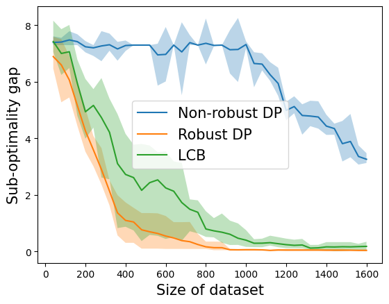
(a) Garnet Problem under global coverage

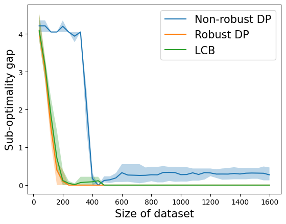
(b) Garnet Problem under partial coverage

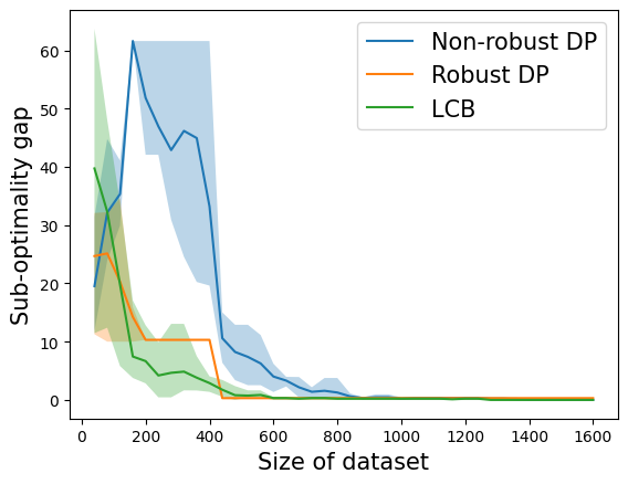
(c) Frozen-Lake under global coverage

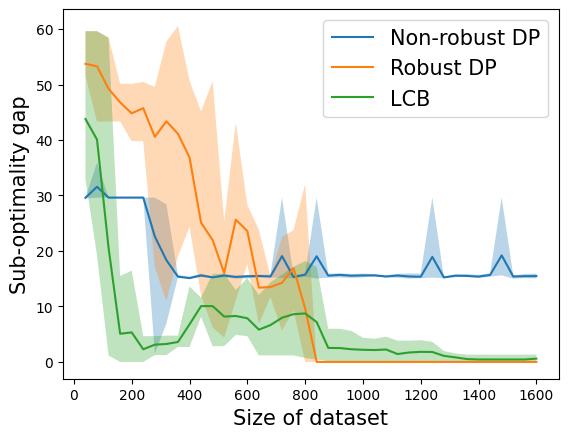
(d) Frozen-Lake under partial coverage

Figure 1: Sub-optimality gaps of Robust DP, LCB approach, and Non-robust DP.

5 Conclusion

In this paper, we revisit the problem of offline reinforcement learning from a novel angle of distributional robustness. We develop a DRO-based approach to solve offline reinforcement learning. Our approach directly incorporates conservatism in estimating the transition dynamics instead of penalizing the reward of less-visited state-action pairs. Our algorithms are based on the robust dynamic programming approach, which is computationally efficient. We focus on the challenging partial coverage setting, and develop two uncertainty sets: the Hoeffding-style and the less conservative Bernstein-style. For the Hoeffding-style uncertainty set, we theoretically characterize its sample complexity, and show it matches with the best one of the LCB-based approaches using the Hoeffding-style bonus term. For the Bernstein-style uncertainty set, we show its sample complexity is minimax optimal. Our results provide a DRO-based framework to efficiently and effectively solve the problem of offline reinforcement learning.

Appendix A Notations

We first introduce some notations that are used in our proofs. We denote the numbers of states and actions by $S,A$, i.e., $|\mathcal{S}|=S$, $|\mathcal{A}|=A$. For a transition kernel $\mathsf{P}$ and a policy $\pi$, $\mathsf{P}^{\pi}$ denotes the transition matrix induced by them, i.e., $\mathsf{P}^{\pi}(s)=\sum_{a}\pi(a|s)\mathsf{P}^{a}_{s}\in\Delta(\mathcal{S})$.

For any vector $V\in\mathbb{R}^{S}$, $V\circ V\in\mathbb{R}^{S}$ denotes the entry-wise multiplication, i.e., $V\circ V(s)=V(s)*V(s)$. For a distribution $q\in\Delta(\mathcal{S})$, it is straightforward to verify that the variance of $V$ w.r.t. $q$ can be rewritten as $\textbf{Var}_{q}(V)=q(V\circ V)-(qV)^{2}$.

Appendix B A Straightforward Analysis: Hoeffding’s Inequality

Lemma 2.

([12, 66]) With probability at least $1-\delta$, it holds that for any $s,a$, $\mathsf{P}^{a}_{s}\in\hat{\mathcal{P}}^{a}_{s}$.

Theorem 3.

(Restatement of Thm 1) With probability at least $1-2\delta$, it holds that

$$V^{\pi^{*}}_{\mathsf{P}}(\rho)-V^{\pi_{r}}_{\mathsf{P}}(\rho)\leq\frac{2}{(1-\gamma)^{2}}\frac{8SC^{\pi^{*}}\log\frac{NS}{\delta}}{N}+\frac{2}{(1-\gamma)^{2}}\sqrt{\frac{24S^{2}C^{\pi^{*}}\log\frac{SA}{\delta}}{N}},$$ (11)

To obtain an $\epsilon$-optimal policy, a dataset of size

$$N=\mathcal{O}\left(\frac{SC^{\pi^{*}}}{(1-\gamma)^{4}\epsilon^{2}}\right)$$ (12)

is required.

Proof.

In the following proof, we only focus on the case when

$$N>\frac{8SC^{\pi^{*}}\log\frac{NS}{\delta}}{1-\gamma};$$ (13)

Otherwise, eq. 6 follows directly from the trivial bound $V^{\pi^{*}}_{\mathsf{P}}(\rho)-V^{\pi_{r}}_{\mathsf{P}}(\rho)\leq\frac{1}{1-\gamma}$.

According to Lemma 1, with probability at least $1-\delta$, $\mathsf{P}\in\hat{\mathcal{P}}$. Moreover, due to the fact $r(s,a)\geq\hat{r}(s,a)$, hence

$$V^{\pi}_{\mathsf{P}}(s)\geq V^{\pi}_{\hat{r},\mathsf{P}}(s)\geq V^{\pi}_{\hat{r},\hat{\mathcal{P}}}(s)=V^{\pi}_{\hat{\mathcal{P}}}(s)$$ (14)

for any $\pi$ and $s\in\mathcal{S}$, where $V^{\pi}_{\hat{r},\mathsf{P}}$ denotes the value function w.r.t. $\mathsf{P}$ and reward $\hat{r}$. Thus $V^{\pi}_{\mathsf{P}}\geq V^{\pi}_{\hat{\mathcal{P}}}$ for any policy $\pi$.

Therefore,

$$V^{\pi^{*}}_{\mathsf{P}}(s)-V^{\pi_{r}}_{\mathsf{P}}(s)$$

$$=V^{\pi^{*}}_{\mathsf{P}}(s)-V^{\pi_{r}}_{\hat{\mathcal{P}}}(s)+V^{\pi_{r}}_{\hat{\mathcal{P}}}(s)-V^{\pi_{r}}_{\mathsf{P}}(s)$$

$$\leq V^{\pi^{*}}_{\mathsf{P}}(s)-V^{\pi_{r}}_{\hat{\mathcal{P}}}(s)$$

$$=r(s,\pi^{*}(s))+\gamma\mathsf{P}^{\pi^{*}(s)}_{s}V^{\pi^{*}}_{\mathsf{P}}-V^{\pi_{r}}_{\hat{\mathcal{P}}}(s)$$

$$\overset{(a)}{\leq}r(s,\pi^{*}(s))-\hat{r}(s,\pi^{*}(s))+\gamma\mathsf{P}^{\pi^{*}(s)}_{s}V^{\pi^{*}}_{\mathsf{P}}-\gamma\sigma_{\hat{\mathcal{P}}^{\pi^{*}(s)}_{s}}(V^{\pi_{r}}_{\hat{\mathcal{P}}})$$

$$=r(s,\pi^{*}(s))-\hat{r}(s,\pi^{*}(s))+\gamma\mathsf{P}^{\pi^{*}(s)}_{s}V^{\pi^{*}}_{\mathsf{P}}-\gamma\mathsf{P}^{\pi^{*}(s)}_{s}V^{\pi_{r}}_{\hat{\mathcal{P}}}+\gamma\mathsf{P}^{\pi^{*}(s)}_{s}V^{\pi_{r}}_{\hat{\mathcal{P}}}-\gamma\sigma_{\hat{\mathcal{P}}^{\pi^{*}(s)}_{s}}(V^{\pi_{r}}_{\hat{\mathcal{P}}})$$

$$=r(s,\pi^{*}(s))-\hat{r}(s,\pi^{*}(s))+\gamma\mathsf{P}^{\pi^{*}(s)}_{s}(V^{\pi^{*}}_{\mathsf{P}}-V^{\pi_{r}}_{\hat{\mathcal{P}}})+\gamma(\mathsf{P}^{\pi^{*}(s)}_{s}V^{\pi_{r}}_{\hat{\mathcal{P}}}-\sigma_{\hat{\mathcal{P}}^{\pi^{*}(s)}_{s}}(V^{\pi_{r}}_{\hat{\mathcal{P}}}))$$

$$\triangleq\gamma\mathsf{P}^{\pi^{*}(s)}_{s}(V^{\pi^{*}}_{\mathsf{P}}-V^{\pi_{r}}_{\hat{\mathcal{P}}})+b^{*}(V^{\pi_{r}}_{\hat{\mathcal{P}}}),$$ (15)

where $(a)$ is from $V^{\pi_{r}}_{\hat{\mathcal{P}}}(s)=\max_{a}Q^{\pi_{r}}_{\hat{\mathcal{P}}}(s,a)\geq Q^{\pi_{r}}_{\hat{\mathcal{P}}}(s,\pi^{*}(s))=\hat{r}(s,\pi^{*}(s))+\gamma\sigma_{\hat{\mathcal{P}}^{\pi^{*}(s)}_{s}}(V^{\pi_{r}}_{\hat{\mathcal{P}}})$, and $b^{*}(V)(s)\triangleq r(s,\pi^{*}(s))-\hat{r}(s,\pi^{*}(s))+\gamma\mathsf{P}^{\pi^{*}(s)}_{s}V-\gamma\sigma_{\hat{\mathcal{P}}^{\pi^{*}(s)}_{s}}(V)$.

Recursively applying this inequality further implies

$$V^{\pi^{*}}_{\mathsf{P}}(\rho)-V^{\pi_{r}}_{\mathsf{P}}(\rho)\leq\frac{1}{1-\gamma}\left\langle d^{\pi^{*}},b^{*}(V^{\pi_{r}}_{\hat{\mathcal{P}}})\right\rangle,$$ (16)

where $d^{\pi^{*}}(\cdot)=(1-\gamma)\sum^{\infty}_{t=0}\gamma^{t}\mathbb{P}(S_{t}=\cdot|S_{0}\sim\rho,\pi^{*},\mathsf{P})$ is the discounted visitation distribution induced by $\pi^{*}$ and $\mathsf{P}$.

To bound the term in appendix B, we introduce the following notations.

$$\mathcal{S}_{s} \triangleq\left\{s:N\mu(s,\pi^{*}(s))\leq 8\log\frac{NS}{\delta}\right\},$$ (17)

$$\mathcal{S}_{l} \triangleq\left\{s:N\mu(s,\pi^{*}(s))>8\log\frac{NS}{\delta}\right\}.$$ (18)

For $s\in\mathcal{S}_{s}$, from eq. 13, we have that

$$\min\left\{d^{\pi^{*}}(s),\frac{1}{S}\right\}\leq C^{\pi^{*}}\mu(s,\pi^{*}(s))\leq\frac{8C^{\pi^{*}}\log\frac{NS}{\delta}}{N}<\frac{1}{S},$$ (19)

which further implies that $d^{\pi^{*}}(s)\leq\frac{8C^{\pi^{*}}\log\frac{NS}{\delta}}{N}$. Hence

$$\sum_{s\in\mathcal{S}_{s}}d^{\pi^{*}}(s)b^{*}(V^{\pi_{r}}_{\hat{\mathcal{P}}})(s)\leq\frac{2}{1-\gamma}\frac{8SC^{\pi^{*}}\log\frac{NS}{\delta}}{N},$$ (20)

which is due to $b^{*}(V)(s)\triangleq r(s,\pi^{*}(s))-\hat{r}(s,\pi^{*}(s))+\gamma\mathsf{P}^{\pi^{*}(s)}_{s}V-\gamma\sigma_{\hat{\mathcal{P}}^{\pi^{*}(s)}_{s}}(V)\leq 1+\frac{\gamma}{1-\gamma}\leq\frac{2}{1-\gamma}$.

We then consider $s\in\mathcal{S}_{l}$. From the definition, $N\mu(s,\pi^{*}(s))>8\log\frac{NS}{\delta}$. According to Lemma 5, with probability $1-\delta$,

$$\max\{12N(s,\pi^{*}(s)),8\log\frac{NS}{\delta}\}\geq N\mu(s,\pi^{*}(s))>8\log\frac{NS}{\delta},$$ (21)

hence $\max\{12N(s,\pi^{*}(s)),8\log\frac{NS}{\delta}\}=12N(s,\pi^{*}(s))$ and $N(s,\pi^{*}(s))\geq\frac{2}{3}\log\frac{NS}{\delta}>0.$ This hence implies that for any $s\in\mathcal{S}_{l}$, $N(s,\pi^{*}(s))>0$ and $\hat{r}(s,\pi^{*}(s))=r(s,\pi^{*}(s))$. Thus

$$|b^{*}(V^{\pi_{r}}_{\hat{\mathcal{P}}})(s)| =\gamma|\mathsf{P}^{\pi^{*}(s)}_{s}V^{\pi_{r}}_{\hat{\mathcal{P}}}-\sigma_{\hat{\mathcal{P}}^{\pi^{*}(s)}_{s}}(V^{\pi_{r}}_{\hat{\mathcal{P}}})|$$

$$\leq\|\mathsf{P}^{\pi^{*}(s)}_{s}-\mathsf{Q}^{\pi^{*}(s)}_{s}\|_{1}\|V^{\pi_{r}}_{\hat{\mathcal{P}}}\|_{\infty}$$

$$\leq\frac{2}{1-\gamma}\min\left\{2,\sqrt{\frac{S\log\frac{SA}{\delta}}{2N(s,\pi^{*}(s))}}\right\}$$

$$\leq\frac{1}{1-\gamma}\sqrt{\frac{2S\log\frac{SA}{\delta}}{N(s,\pi^{*}(s))}}.$$ (22)

Moreover, from eq. 21,

$$\frac{1}{N(s,\pi^{*}(s))}\leq\frac{12}{N\mu(s,\pi^{*}(s))}\leq\frac{12C^{\pi^{*}}}{N\min\{d^{\pi^{*}}(s),\frac{1}{S}\}}\leq\frac{12C^{\pi^{*}}}{N}\left(\frac{1}{d^{\pi^{*}}(s)}+S\right).$$ (23)

Combining with appendix B further implies

$$|b^{*}(V^{\pi_{r}}_{\hat{\mathcal{P}}})(s)| \leq\frac{1}{1-\gamma}\sqrt{2S\log\frac{SA}{\delta}}\sqrt{\frac{12C^{\pi^{*}}}{N}\left(\frac{1}{d^{\pi^{*}}(s)},S\right)}$$

$$\leq\frac{1}{1-\gamma}\sqrt{2S\log\frac{SA}{\delta}}\sqrt{\frac{12C^{\pi^{*}}}{N}\frac{1}{d^{\pi^{*}}(s)}}+\frac{1}{1-\gamma}\sqrt{2S\log\frac{SA}{\delta}}\sqrt{\frac{12C^{\pi^{*}}}{N}S}.$$ (24)

Thus

$$\sum_{s\in\mathcal{S}_{l}}d^{\pi^{*}}(s)b^{*}(V^{\pi_{r}}_{\hat{\mathcal{P}}})(s) \leq\frac{1}{1-\gamma}\sqrt{\frac{24SC^{\pi^{*}}\log\frac{SA}{\delta}}{N}}\sum_{s}\sqrt{d^{\pi^{*}}(s)}+\frac{1}{1-\gamma}\sqrt{\frac{24S^{2}C^{\pi^{*}}\log\frac{SA}{\delta}}{N}}$$

$$\leq\frac{1}{1-\gamma}\sqrt{\frac{24S^{2}C^{\pi^{*}}\log\frac{2}{\delta}}{N}}+\frac{1}{1-\gamma}\sqrt{\frac{24S^{2}C^{\pi^{*}}\log\frac{SA}{\delta}}{N}}$$

$$=\frac{2}{1-\gamma}\sqrt{\frac{24S^{2}C^{\pi^{*}}\log\frac{SA}{\delta}}{N}}.$$ (25)

Thus combining eq. 20 and appendix B implies

$$V^{\pi^{*}}_{\mathsf{P}}(\rho)-V^{\pi_{r}}_{\mathsf{P}}(\rho)$$

$$\leq\frac{1}{1-\gamma}\left\langle d^{\pi^{*}},b^{*}(V^{\pi_{r}}_{\hat{\mathcal{P}}})\right\rangle$$

$$\leq\frac{2}{(1-\gamma)^{2}}\frac{8SC^{\pi^{*}}\log\frac{NS}{\delta}}{N}+\frac{2}{(1-\gamma)^{2}}\sqrt{\frac{24S^{2}C^{\pi^{*}}\log\frac{SA}{\delta}}{N}},$$ (26)

which completes the proof. ∎

Appendix C A Refined Analysis: Bernstein’s Inequality

In this section, we provide a refined analysis of the sub-optimality gap using Bernstein’s Inequality.

Theorem 4.

(Restatement of Thm 2) Consider the robust MDP $\hat{\mathcal{M}}$, there exist an optimal policy $\pi_{r}$ such that there exists some universal constants $K_{1},K_{2}$, such that with probability at least $1-4\delta$, if $N\geq\frac{1}{(1-\gamma)KSC^{\pi^{*}}\mu^{2}_{\min}}$, it holds that

$$V^{\pi^{*}}_{\mathsf{P}}(\rho)-V^{\pi_{r}}_{\mathsf{P}}(\rho)\leq\sqrt{\frac{K_{2}SC^{\pi^{*}}\log\frac{4N}{\delta}}{(1-\gamma)^{3}N}}+\frac{384\log^{2}\frac{4SAN}{(1-\gamma)\delta}}{(1-\gamma)^{2}N\mu_{\min}},$$ (27)

where $K_{2}=442368$.

Proof.

We first have that

$$V^{\pi^{*}}_{\mathsf{P}}-V^{\pi_{r}}_{\mathsf{P}} =\underbrace{V^{\pi^{*}}_{\mathsf{P}}-V^{\pi_{r}}_{\hat{\mathcal{P}}}}_{\Delta_{1}}+\underbrace{V^{\pi_{r}}_{\hat{\mathcal{P}}}-V^{\pi_{r}}_{\mathsf{P}}}_{\Delta_{2}}.$$ (28)

In the following proof, we only focus on the case when

$$N>\max\left\{\frac{SK_{1}C^{\pi^{*}}\log\frac{NS}{\delta}}{1-\gamma},\frac{1}{(1-\gamma)KSC^{\pi^{*}}\mu^{2}_{\min}}\right\};$$ (29)

Otherwise, eq. 8 follows directly from the trivial bound $V^{\pi^{*}}_{\mathsf{P}}(\rho)-V^{\pi_{r}}_{\mathsf{P}}(\rho)\leq\frac{1}{1-\gamma}$.

We note that Lemma 8 of [56] states that under eq. 29, with probability $1-\delta$, for any $(s,a)$ pair,

$$N(s,a)\geq\frac{N\mu(s,a)}{8\log\frac{4SA}{\delta}}.$$ (30)

This moreover implies that with probability $1-\delta$, if $\mu(s,a)>0$, then $N(s,a)>0$. We hence focus on the case when this event holds.

The remaining proof can be completed by combining the following two theorems. ∎

Theorem 5.

With probability at least $1-2\delta$, it holds that

$$\rho^{\top}\Delta_{1}\leq{\frac{2c_{2}SC^{\pi^{*}}\log\frac{4N}{\delta}}{(1-\gamma)^{2}N}}+\frac{80Sc_{1}C^{\pi^{*}}\log\frac{NS}{\delta}}{(1-\gamma)^{2}N}+\frac{96}{\gamma}\sqrt{\frac{48SC^{\pi^{*}}\log\frac{4N}{\delta}}{(1-\gamma)^{3}N}}.$$ (31)

Proof.

We first define the following set:

$$\mathcal{S}_{0}\triangleq\{s:d^{\pi^{*}}(s)=0\}.$$ (32)

And for $s\notin\mathcal{S}_{0}$, it holds that $d^{\pi^{*}}(s)>0$.

We first consider $s\notin\mathcal{S}_{0}$. Due to the fact $d^{\pi^{*}}(s)>0$, hence $d^{\pi^{*}}(s,\pi^{*}(s))=d^{\pi^{*}}(s)\pi^{*}(\pi^{*}(s)|s)>0$. Thus it implies that $\mu(s,\pi^{*}(s))>0$, and (30) further implies $N(s,\pi^{*}(s))>0$ and $\hat{r}(s,\pi^{*}(s))=r(s,\pi^{*}(s))$. Hence we have that

$$V^{\pi^{*}}_{\mathsf{P}}(s)-V^{\pi_{r}}_{\hat{\mathcal{P}}}(s) =r(s,\pi^{*}(s))+\gamma\mathsf{P}^{\pi^{*}(s)}_{s}V^{\pi^{*}}_{\mathsf{P}}-V^{\pi_{r}}_{\hat{\mathcal{P}}}(s)$$

$$\overset{(a)}{\leq}\gamma\mathsf{P}^{\pi^{*}(s)}_{s}V^{\pi^{*}}_{\mathsf{P}}-\gamma\sigma_{\hat{\mathcal{P}}^{\pi^{*}(s)}_{s}}(V^{\pi_{r}}_{\hat{\mathcal{P}}})$$

$$=\gamma\mathsf{P}^{\pi^{*}(s)}_{s}V^{\pi^{*}}_{\mathsf{P}}-\gamma\mathsf{P}^{\pi^{*}(s)}_{s}V^{\pi_{r}}_{\hat{\mathcal{P}}}+\gamma\mathsf{P}^{\pi^{*}(s)}_{s}V^{\pi_{r}}_{\hat{\mathcal{P}}}-\gamma\sigma_{\hat{\mathcal{P}}^{\pi^{*}(s)}_{s}}(V^{\pi_{r}}_{\hat{\mathcal{P}}})$$

$$=\gamma\mathsf{P}^{\pi^{*}(s)}_{s}(V^{\pi^{*}}_{\mathsf{P}}-V^{\pi_{r}}_{\hat{\mathcal{P}}})+\gamma(\mathsf{P}^{\pi^{*}(s)}_{s}V^{\pi_{r}}_{\hat{\mathcal{P}}}-\sigma_{\hat{\mathcal{P}}^{\pi^{*}(s)}_{s}}(V^{\pi_{r}}_{\hat{\mathcal{P}}})),$$ (33)

where $(a)$ is from $V^{\pi_{r}}_{\hat{\mathcal{P}}}(s)=\max_{a}Q^{\pi_{r}}_{\hat{\mathcal{P}}}(s,a)\geq Q^{\pi_{r}}_{\hat{\mathcal{P}}}(s,\pi^{*}(s))=\hat{r}(s,\pi^{*}(s))+\gamma\sigma_{\hat{\mathcal{P}}^{\pi^{*}(s)}_{s}}(V^{\pi_{r}}_{\hat{\mathcal{P}}})=r(s,\pi^{*}(s))+\gamma\sigma_{\hat{\mathcal{P}}^{\pi^{*}(s)}_{s}}(V^{\pi_{r}}_{\hat{\mathcal{P}}})$.

For $s\in\mathcal{S}_{0}$, it holds that

$$V^{\pi^{*}}_{\mathsf{P}}(s)-V^{\pi_{r}}_{\hat{\mathcal{P}}}(s) =r(s,\pi^{*}(s))+\gamma\mathsf{P}^{\pi^{*}(s)}_{s}V^{\pi^{*}}_{\mathsf{P}}-V^{\pi_{r}}_{\hat{\mathcal{P}}}(s)$$

$$\overset{(a)}{\leq}\gamma\mathsf{P}^{\pi^{*}(s)}_{s}V^{\pi^{*}}_{\mathsf{P}}-\gamma\sigma_{\hat{\mathcal{P}}^{\pi^{*}(s)}_{s}}(V^{\pi_{r}}_{\hat{\mathcal{P}}})+r(s,\pi^{*}(s))-\hat{r}(s,\pi^{*}(s))$$

$$\leq\gamma\mathsf{P}^{\pi^{*}(s)}_{s}(V^{\pi^{*}}_{\mathsf{P}}-V^{\pi_{r}}_{\hat{\mathcal{P}}})+\gamma(\mathsf{P}^{\pi^{*}(s)}_{s}V^{\pi_{r}}_{\hat{\mathcal{P}}}-\sigma_{\hat{\mathcal{P}}^{\pi^{*}(s)}_{s}}(V^{\pi_{r}}_{\hat{\mathcal{P}}}))+1,$$ (34)

where $(a)$ follows similarly from appendix C, and the last inequality is from $r(s,\pi^{*}(s))\leq 1$.

Hence combining appendix C and appendix C implies

$$V^{\pi^{*}}_{\mathsf{P}}(s)-V^{\pi_{r}}_{\hat{\mathcal{P}}}(s)\leq\gamma\mathsf{P}^{\pi^{*}(s)}_{s}(V^{\pi^{*}}_{\mathsf{P}}-V^{\pi_{r}}_{\hat{\mathcal{P}}})+b^{*}(V)(s),$$ (35)

where $b^{*}(V)(s)\triangleq\gamma\mathsf{P}^{\pi^{*}(s)}_{s}V-\gamma\sigma_{\hat{\mathcal{P}}^{\pi^{*}(s)}_{s}}(V)$ if $s\notin\mathcal{S}_{0}$, and $b^{*}(V)(s)\triangleq 1+\gamma\mathsf{P}^{\pi^{*}(s)}_{s}V-\gamma\sigma_{\hat{\mathcal{P}}^{\pi^{*}(s)}_{s}}(V)$ for $s\in\mathcal{S}_{0}$.

Moreover we set

$$\tilde{b}(V^{\pi_{r}}_{\hat{\mathcal{P}}})(s)=\max\{0,b^{*}(V^{\pi_{r}}_{\hat{\mathcal{P}}})(s)\},$$ (36)

then it holds that $b^{*}(V^{\pi_{r}}_{\hat{\mathcal{P}}})\leq\tilde{b}(V^{\pi_{r}}_{\hat{\mathcal{P}}})$.

Then apply eq. 35 recursively and we have that

$$\rho^{\top}\Delta_{1}\leq\frac{1}{1-\gamma}\left\langle d^{\pi^{*}},\tilde{b}(V^{\pi_{r}}_{\hat{\mathcal{P}}})\right\rangle,$$ (37)

Not that for $s\in\mathcal{S}_{0}$, it holds that $d^{\pi^{*}}(s)=0$, and

$$\left\langle d^{\pi^{*}},\tilde{b}(V^{\pi_{r}}_{\hat{\mathcal{P}}})\right\rangle=\sum_{s\notin\mathcal{S}_{0}}d^{\pi^{*}}(s)\tilde{b}(V^{\pi_{r}}_{\hat{\mathcal{P}}})(s).$$ (38)

This implies that we only need to focus on $s\notin\mathcal{S}_{0}$. We further defined the following sets:

$$\mathcal{S}_{s} \triangleq\left\{s\notin\mathcal{S}_{0}:N\mu(s,\pi^{*}(s))\leq 8\log\frac{NS}{\delta}\right\},$$ (39)

$$\mathcal{S}_{l} \triangleq\left\{s\notin\mathcal{S}_{0}:N\mu(s,\pi^{*}(s))>8\log\frac{NS}{\delta}\right\}.$$ (40)

For $s\in\mathcal{S}_{s}$, we have that

$$\min\left\{d^{\pi^{*}}(s),\frac{1}{S}\right\}\leq C^{\pi^{*}}\mu(s,\pi^{*}(s))\leq\frac{8C^{\pi^{*}}\log\frac{NS}{\delta}}{N}\overset{(a)}{<}\frac{1}{S},$$ (41)

where $(a)$ is due to the fact eq. 29.

This further implies that $d^{\pi^{*}}(s)\leq\frac{8C^{\pi^{*}}\log\frac{NS}{\delta}}{N}$. Hence

$$\sum_{s\in\mathcal{S}_{s}}d^{\pi^{*}}(s)\tilde{b}(V^{\pi_{r}}_{\hat{\mathcal{P}}})(s)\leq\frac{2}{1-\gamma}\frac{8SC^{\pi^{*}}\log\frac{NS}{\delta}}{N},$$ (42)

which is due to $\|\mathsf{P}^{\pi^{*}(s)}_{s}V^{\pi_{r}}_{\hat{\mathcal{P}}}-\sigma_{\hat{\mathcal{P}}^{\pi^{*}(s)}_{s}}(V^{\pi_{r}}_{\hat{\mathcal{P}}})\|\leq\frac{2}{1-\gamma}$.

We then consider $s\in\mathcal{S}_{l}$. Note that from the definition and (30), it holds that $N(s,\pi^{*}(s))>0$ for $s\in\mathcal{S}_{l}$.

Therefore it holds that

$$\tilde{b}(V^{\pi_{r}}_{\hat{\mathcal{P}}})(s) \leq|\gamma\mathsf{P}^{\pi^{*}(s)}_{s}V^{\pi_{r}}_{\hat{\mathcal{P}}}-\gamma\sigma_{\hat{\mathcal{P}}^{\pi^{*}(s)}_{s}}(V^{\pi_{r}}_{\hat{\mathcal{P}}})|$$

$$\leq|\gamma\mathsf{P}^{\pi^{*}(s)}_{s}V^{\pi_{r}}_{\hat{\mathcal{P}}}-\gamma\hat{\mathsf{P}}^{\pi^{*}(s)}_{s}V^{\pi_{r}}_{\hat{\mathcal{P}}}|+|\gamma\hat{\mathsf{P}}^{\pi^{*}(s)}_{s}V^{\pi_{r}}_{\hat{\mathcal{P}}}-\gamma\sigma_{\hat{\mathcal{P}}^{\pi^{*}(s)}_{s}}(V^{\pi_{r}}_{\hat{\mathcal{P}}})|$$

$$\leq\gamma\big{|}\mathsf{P}^{\pi^{*}(s)}_{s}V^{\pi_{r}}_{\hat{\mathcal{P}}}-\hat{\mathsf{P}}^{\pi^{*}(s)}_{s}V^{\pi_{r}}_{\hat{\mathcal{P}}}\big{|}+\sqrt{\frac{\log\frac{4N}{\delta}\textbf{Var}_{\hat{\mathsf{P}}^{\pi^{*}(s)}_{s}}(V^{\pi_{r}}_{\hat{\mathcal{P}}})}{N(s,\pi^{*}(s))}},$$ (43)

where the last inequality is shown as follows.

Since $\hat{\mathsf{P}}^{\pi^{*}(s)}_{s}\in\hat{\mathcal{P}}^{a}_{s}$, we have that $\hat{\mathsf{P}}^{\pi^{*}(s)}_{s}V^{\pi_{r}}_{\hat{\mathcal{P}}}\geq\sigma_{\hat{\mathcal{P}}^{\pi^{*}(s)}_{s}}(V^{\pi_{r}}_{\hat{\mathcal{P}}})$. Now note that it is shown in [27, 58] that

$$\sigma_{\hat{\mathcal{P}}^{\pi^{*}(s)}_{s}}(V^{\pi_{r}}_{\hat{\mathcal{P}}})=\max_{\mu\in[0,V^{\pi_{r}}_{\hat{\mathcal{P}}}]}\left\{\hat{\mathsf{P}}^{\pi^{*}(s)}_{s}(V^{\pi_{r}}_{\hat{\mathcal{P}}}-\mu)-\sqrt{R^{\pi^{*}(s)}_{s}\textbf{Var}_{\hat{\mathsf{P}}^{\pi^{*}(s)}_{s}}(V^{\pi_{r}}_{\hat{\mathcal{P}}}-\mu)}\right\}.$$ (44)

Thus

$$|\gamma\hat{\mathsf{P}}^{\pi^{*}(s)}_{s}V^{\pi_{r}}_{\hat{\mathcal{P}}}-\gamma\sigma_{\hat{\mathcal{P}}^{\pi^{*}(s)}_{s}}(V^{\pi_{r}}_{\hat{\mathcal{P}}})|$$

$$=\gamma\hat{\mathsf{P}}^{\pi^{*}(s)}_{s}V^{\pi_{r}}_{\hat{\mathcal{P}}}-\gamma\sigma_{\hat{\mathcal{P}}^{\pi^{*}(s)}_{s}}(V^{\pi_{r}}_{\hat{\mathcal{P}}})$$

$$=\gamma\hat{\mathsf{P}}^{\pi^{*}(s)}_{s}V^{\pi_{r}}_{\hat{\mathcal{P}}}-\gamma\max_{\mu\in[0,V^{\pi_{r}}_{\hat{\mathcal{P}}}]}\left\{\hat{\mathsf{P}}^{\pi^{*}(s)}_{s}(V^{\pi_{r}}_{\hat{\mathcal{P}}}-\mu)-\sqrt{R^{\pi^{*}(s)}_{s}\textbf{Var}_{\hat{\mathsf{P}}^{\pi^{*}(s)}_{s}}(V^{\pi_{r}}_{\hat{\mathcal{P}}}-\mu)}\right\}$$

$$\overset{(a)}{\leq}\gamma\hat{\mathsf{P}}^{\pi^{*}(s)}_{s}V^{\pi_{r}}_{\hat{\mathcal{P}}}-\gamma\left(\hat{\mathsf{P}}^{\pi^{*}(s)}_{s}(V^{\pi_{r}}_{\hat{\mathcal{P}}})-\sqrt{R^{\pi^{*}(s)}_{s}\textbf{Var}_{\hat{\mathsf{P}}^{\pi^{*}(s)}_{s}}(V^{\pi_{r}}_{\hat{\mathcal{P}}})}\right)$$

$$=\sqrt{R^{\pi^{*}(s)}_{s}\textbf{Var}_{\hat{\mathsf{P}}^{\pi^{*}(s)}_{s}}(V^{\pi_{r}}_{\hat{\mathcal{P}}})},$$ (45)

where $(a)$ is due to the maximum term is larger than the function value at $\mu=0$, and this inequality completes the proof of Appendix C.

To further bound appendix C, we invoke Lemma 7 and have that

$$\big{|}\mathsf{P}^{\pi^{*}(s)}_{s}V^{\pi_{r}}_{\hat{\mathcal{P}}}-\hat{\mathsf{P}}^{\pi^{*}(s)}_{s}V^{\pi_{r}}_{\hat{\mathcal{P}}}\big{|}$$

$$\leq 12\sqrt{\frac{\textbf{Var}_{\hat{\mathsf{P}}^{\pi^{*}(s)}_{s}}(V^{\pi_{r}}_{\hat{\mathcal{P}}})\log\frac{4N}{\delta}}{N(s,\pi^{*}(s))}}+\frac{74\log\frac{4N}{\delta}}{(1-\gamma)N(s,\pi^{*}(s))}$$

$$\leq 12\sqrt{\frac{\log\frac{4N}{\delta}}{N(s,\pi^{*}(s))}\left(2\textbf{Var}_{\mathsf{P}^{\pi^{*}(s)}_{s}}(V^{\pi_{r}}_{\hat{\mathcal{P}}})+\frac{41\log\frac{4N}{\delta}}{(1-\gamma)^{2}N(s,\pi^{*}(s))}\right)}+\frac{74\log\frac{4N}{\delta}}{(1-\gamma)N(s,\pi^{*}(s))}$$

$$\leq 12\sqrt{\frac{2\log\frac{4N}{\delta}}{N(s,\pi^{*}(s))}\textbf{Var}_{\mathsf{P}^{\pi^{*}(s)}_{s}}(V^{\pi_{r}}_{\hat{\mathcal{P}}})}+\frac{(74+12\sqrt{41})\log\frac{4N}{\delta}}{(1-\gamma)N(s,\pi^{*}(s))},$$ (46)

where the last inequality is from $\sqrt{x+y}\leq\sqrt{x}+\sqrt{y}$.

Combine appendix C and appendix C, we further have that

$$\tilde{b}(V^{\pi_{r}}_{\hat{\mathcal{P}}})(s) \leq 24\sqrt{\frac{2\log\frac{4N}{\delta}}{N(s,\pi^{*}(s))}\textbf{Var}_{\mathsf{P}^{\pi^{*}(s)}_{s}}(V^{\pi_{r}}_{\hat{\mathcal{P}}})}+\frac{(74+12\sqrt{41})\log\frac{4N}{\delta}}{(1-\gamma)N(s,\pi^{*}(s))}+\frac{\log\frac{N}{\delta}}{(1-\gamma)N(s,\pi^{*}(s))}$$

$$\leq 24\sqrt{\frac{2\log\frac{4N}{\delta}}{N(s,\pi^{*}(s))}\textbf{Var}_{\mathsf{P}^{\pi^{*}(s)}_{s}}(V^{\pi_{r}}_{\hat{\mathcal{P}}})}+\frac{c_{1}\log\frac{4N}{\delta}}{(1-\gamma)N(s,\pi^{*}(s))},$$ (47)

where $c_{1}=75+12\sqrt{41}$.

Note that in eq. 23, we showed that $\frac{1}{N(s,\pi^{*}(s))}\leq\frac{12C^{\pi^{*}}}{N}(S+\frac{1}{d^{\pi^{*}}(s)})$. Hence plugging in appendix C implies that

$$\tilde{b}(V^{\pi_{r}}_{\hat{\mathcal{P}}})(s)\leq 24\sqrt{\frac{24C^{\pi^{*}}\log\frac{4N}{\delta}}{N}\textbf{Var}_{\mathsf{P}^{\pi^{*}(s)}_{s}}(V^{\pi_{r}}_{\hat{\mathcal{P}}})}\left(\sqrt{S}+\frac{1}{\sqrt{d^{\pi^{*}}(s)}}\right)$$

$$\quad+\frac{12c_{1}C^{\pi^{*}}\log\frac{4N}{\delta}}{(1-\gamma)N}\left(S+\frac{1}{d^{\pi^{*}}(s)}\right).$$ (48)

Firstly we have that

$$\sum_{s\in\mathcal{S}_{l}}24d^{\pi^{*}}(s)\sqrt{\frac{24C^{\pi^{*}}\log\frac{4N}{\delta}}{N}\textbf{Var}_{\mathsf{P}^{\pi^{*}(s)}_{s}}(V^{\pi_{r}}_{\hat{\mathcal{P}}})}\left(\sqrt{S}+\frac{1}{\sqrt{d^{\pi^{*}}(s)}}\right)$$

$$=\sum_{s\in\mathcal{S}_{l}}24d^{\pi^{*}}(s)\sqrt{\frac{24SC^{\pi^{*}}\log\frac{4N}{\delta}}{N}\textbf{Var}_{\mathsf{P}^{\pi^{*}(s)}_{s}}(V^{\pi_{r}}_{\hat{\mathcal{P}}})}+\sum_{s\in\mathcal{S}_{l}}12\sqrt{d^{\pi^{*}}(s)}\sqrt{\frac{24C^{\pi^{*}}\log\frac{4N}{\delta}}{N}\textbf{Var}_{\mathsf{P}^{\pi^{*}(s)}_{s}}(V^{\pi_{r}}_{\hat{\mathcal{P}}})}$$

$$=24\sqrt{\frac{24C^{\pi^{*}}\log\frac{4N}{\delta}}{N}}\left(\sum_{s\in\mathcal{S}_{l}}\sqrt{d^{\pi^{*}}(s)\textbf{Var}_{\mathsf{P}^{\pi^{*}(s)}_{s}}(V^{\pi_{r}}_{\hat{\mathcal{P}}})}+\sum_{s\in\mathcal{S}_{l}}\sqrt{d^{\pi^{*}}(s)}\sqrt{Sd^{\pi^{*}}(s)\textbf{Var}_{\mathsf{P}^{\pi^{*}(s)}_{s}}(V^{\pi_{r}}_{\hat{\mathcal{P}}})}\right)$$

$$\overset{(a)}{\leq}24\sqrt{\frac{24C^{\pi^{*}}\log\frac{4N}{\delta}}{N}}\left(\sqrt{S}\sqrt{\sum_{s\in\mathcal{S}_{l}}d^{\pi^{*}}(s)\textbf{Var}_{\mathsf{P}^{\pi^{*}(s)}_{s}}(V^{\pi_{r}}_{\hat{\mathcal{P}}})}+\sqrt{\sum_{s\in\mathcal{S}_{l}}Sd^{\pi^{*}}(s)\textbf{Var}_{\mathsf{P}^{\pi^{*}(s)}_{s}}(V^{\pi_{r}}_{\hat{\mathcal{P}}})}\right)$$

$$=48\sqrt{\frac{24SC^{\pi^{*}}\log\frac{4N}{\delta}}{N}}\sqrt{\sum_{s\in\mathcal{S}_{l}}d^{\pi^{*}}(s)\textbf{Var}_{\mathsf{P}^{\pi^{*}(s)}_{s}}(V^{\pi_{r}}_{\hat{\mathcal{P}}})},$$ (49)

where $(a)$ is from Cauchy’s inequality and the fact $\sum_{s\in\mathcal{S}_{l}}d^{\pi^{*}}(s)\leq 1$.

In addition, we have that

$$\sum_{s\in\mathcal{S}_{l}}d^{\pi^{*}}(s)\frac{12c_{1}C^{\pi^{*}}\log\frac{4N}{\delta}}{(1-\gamma)N}\left(S+\frac{1}{d^{\pi^{*}}(s)}\right)\leq\frac{24c_{1}SC^{\pi^{*}}\log\frac{4N}{\delta}}{(1-\gamma)N}.$$ (50)

Combine the two inequalities above and we have that

$$\sum_{s\in\mathcal{S}_{l}}d^{\pi^{*}}(s)\tilde{b}(V^{\pi_{r}}_{\hat{\mathcal{P}}})(s)$$

$$\leq 48\sqrt{\frac{24SC^{\pi^{*}}\log\frac{4N}{\delta}}{N}}\sqrt{\sum_{s\in\mathcal{S}_{l}}d^{\pi^{*}}(s)\textbf{Var}_{\mathsf{P}^{\pi^{*}(s)}_{s}}(V^{\pi_{r}}_{\hat{\mathcal{P}}})}+\frac{24Sc_{1}C^{\pi^{*}}\log\frac{4N}{\delta}}{(1-\gamma)N}.$$ (51)

Then we combine eq. 42 and appendix C, and it implies that

$$\langle d^{\pi^{*}},\tilde{b}(V^{\pi_{r}}_{\hat{\mathcal{P}}})\rangle$$

$$=\sum_{s\in\mathcal{S}_{s}}d^{\pi^{*}}(s)\tilde{b}(V^{\pi_{r}}_{\hat{\mathcal{P}}})(s)+\sum_{s\in\mathcal{S}_{l}}d^{\pi^{*}}(s)\tilde{b}(V^{\pi_{r}}_{\hat{\mathcal{P}}})(s)$$

$$\leq\frac{16SC^{\pi^{*}}\log\frac{NS}{\delta}}{(1-\gamma)N}+48\sqrt{\frac{24SC^{\pi^{*}}\log\frac{4N}{\delta}}{N}}\sqrt{\sum_{s\in\mathcal{S}_{l}}d^{\pi^{*}}(s)\textbf{Var}_{\mathsf{P}^{\pi^{*}(s)}_{s}}(V^{\pi_{r}}_{\hat{\mathcal{P}}})}+\frac{24Sc_{1}C^{\pi^{*}}\log\frac{4N}{\delta}}{(1-\gamma)N}$$

$$\leq\frac{40c_{1}SC^{\pi^{*}}\log\frac{NS}{\delta}}{(1-\gamma)N}+48\sqrt{\frac{24SC^{\pi^{*}}\log\frac{4N}{\delta}}{N}}\sqrt{\sum_{s\in\mathcal{S}}d^{\pi^{*}}(s)\textbf{Var}_{\mathsf{P}^{\pi^{*}(s)}_{s}}(V^{\pi_{r}}_{\hat{\mathcal{P}}})}.$$ (52)

We then bound the term $\sum_{s\in\mathcal{S}}d^{\pi^{*}}(s)\textbf{Var}_{\mathsf{P}^{\pi^{*}(s)}_{s}}(V^{\pi_{r}}_{\hat{\mathcal{P}}})$. We first claim the following inequality:

$$V^{\pi_{r}}_{\hat{\mathcal{P}}}-\gamma\mathsf{P}^{\pi^{*}}V^{\pi_{r}}_{\hat{\mathcal{P}}}+2\tilde{b}(V^{\pi_{r}}_{\hat{\mathcal{P}}})\geq 0.$$ (53)

To prove eq. 53, we note that

$$V^{\pi_{r}}_{\hat{\mathcal{P}}}(s) =\max_{a}Q^{\pi_{r}}_{\hat{\mathcal{P}}}(s,a)$$

$$\geq Q^{\pi_{r}}_{\hat{\mathcal{P}}}(s,\pi^{*}(s))$$

$$=\hat{r}(s,\pi^{*}(s))+\gamma\sigma_{\hat{\mathcal{P}}^{\pi^{*}(s)}_{s}}(V^{\pi_{r}}_{\hat{\mathcal{P}}})$$

$$=\hat{r}(s,\pi^{*}(s))+\gamma\mathsf{P}^{\pi^{*}(s)}_{s}V^{\pi_{r}}_{\hat{\mathcal{P}}}-\gamma\mathsf{P}^{\pi^{*}(s)}_{s}V^{\pi_{r}}_{\hat{\mathcal{P}}}+\gamma\sigma_{\hat{\mathcal{P}}^{\pi^{*}(s)}_{s}}(V^{\pi_{r}}_{\hat{\mathcal{P}}})$$

$$\overset{(a)}{\geq}\hat{r}(s,\pi^{*}(s))+\gamma\mathsf{P}^{\pi^{*}(s)}_{s}V^{\pi_{r}}_{\hat{\mathcal{P}}}-b^{*}(V^{\pi_{r}}_{\hat{\mathcal{P}}})(s)$$

$$\geq\hat{r}(s,\pi^{*}(s))+\gamma\mathsf{P}^{\pi^{*}(s)}_{s}V^{\pi_{r}}_{\hat{\mathcal{P}}}-2\tilde{b}(V^{\pi_{r}}_{\hat{\mathcal{P}}})(s),$$ (54)

where $(a)$ is from $b^{*}(V^{\pi_{r}}_{\hat{\mathcal{P}}})(s)\geq\gamma\mathsf{P}^{\pi^{*}(s)}_{s}V^{\pi_{r}}_{\hat{\mathcal{P}}}-\gamma\sigma_{\hat{\mathcal{P}}^{\pi^{*}(s)}_{s}}(V^{\pi_{r}}_{\hat{\mathcal{P}}})$.

Hence for any $s\in\mathcal{S}$,

$$V^{\pi_{r}}_{\hat{\mathcal{P}}}(s)-\gamma\mathsf{P}^{\pi^{*}(s)}_{s}V^{\pi_{r}}_{\hat{\mathcal{P}}}+2\tilde{b}(V^{\pi_{r}}_{\hat{\mathcal{P}}})(s)\geq\hat{r}(s,\pi^{*}(s))\geq 0,$$ (55)

which proves eq. 53.

Now with eq. 53, we first note that

$$(V^{\pi_{r}}_{\hat{\mathcal{P}}}\circ V^{\pi_{r}}_{\hat{\mathcal{P}}})-(\gamma\mathsf{P}^{\pi^{*}}V^{\pi_{r}}_{\hat{\mathcal{P}}})\circ(\gamma\mathsf{P}^{\pi^{*}}V^{\pi_{r}}_{\hat{\mathcal{P}}})$$

$$=(V^{\pi_{r}}_{\hat{\mathcal{P}}}-\gamma\mathsf{P}^{\pi^{*}}V^{\pi_{r}}_{\hat{\mathcal{P}}})\circ(V^{\pi_{r}}_{\hat{\mathcal{P}}}+\gamma\mathsf{P}^{\pi^{*}}V^{\pi_{r}}_{\hat{\mathcal{P}}})$$

$$\leq(V^{\pi_{r}}_{\hat{\mathcal{P}}}-\gamma\mathsf{P}^{\pi^{*}}V^{\pi_{r}}_{\hat{\mathcal{P}}}+2\tilde{b}(V^{\pi_{r}}_{\hat{\mathcal{P}}}))\circ(V^{\pi_{r}}_{\hat{\mathcal{P}}}+\gamma\mathsf{P}^{\pi^{*}}V^{\pi_{r}}_{\hat{\mathcal{P}}})$$

$$\leq\frac{2}{1-\gamma}(V^{\pi_{r}}_{\hat{\mathcal{P}}}-\gamma\mathsf{P}^{\pi^{*}}V^{\pi_{r}}_{\hat{\mathcal{P}}}+2\tilde{b}(V^{\pi_{r}}_{\hat{\mathcal{P}}})),$$ (56)

where the last inequality is due to the fact $\|V^{\pi_{r}}_{\hat{\mathcal{P}}}+\gamma\mathsf{P}^{\pi^{*}}V^{\pi_{r}}_{\hat{\mathcal{P}}}\|\leq\frac{2}{1-\gamma}$ and eq. 53.

We then have that

$$\sum_{s\in\mathcal{S}}d^{\pi^{*}}(s)\textbf{Var}_{\mathsf{P}^{\pi^{*}(s)}_{s}}(V^{\pi_{r}}_{\hat{\mathcal{P}}})$$

$$=\langle d^{\pi^{*}},\mathsf{P}^{\pi^{*}}(V^{\pi_{r}}_{\hat{\mathcal{P}}}\circ V^{\pi_{r}}_{\hat{\mathcal{P}}})-(\mathsf{P}^{\pi^{*}}V^{\pi_{r}}_{\hat{\mathcal{P}}})\circ(\mathsf{P}^{\pi^{*}}V^{\pi_{r}}_{\hat{\mathcal{P}}})\rangle$$

$$\overset{(a)}{\leq}\left\langle d^{\pi^{*}},\mathsf{P}^{\pi^{*}}(V^{\pi_{r}}_{\hat{\mathcal{P}}}\circ V^{\pi_{r}}_{\hat{\mathcal{P}}})-\frac{1}{\gamma^{2}}(V^{\pi_{r}}_{\hat{\mathcal{P}}}\circ V^{\pi_{r}}_{\hat{\mathcal{P}}})+\frac{2}{\gamma^{2}(1-\gamma)}(V^{\pi_{r}}_{\hat{\mathcal{P}}}-\gamma\mathsf{P}^{\pi^{*}}V^{\pi_{r}}_{\hat{\mathcal{P}}}+2\tilde{b}(V^{\pi_{r}}_{\hat{\mathcal{P}}}))\right\rangle$$

$$\overset{(b)}{\leq}\left\langle d^{\pi^{*}},\mathsf{P}^{\pi^{*}}(V^{\pi_{r}}_{\hat{\mathcal{P}}}\circ V^{\pi_{r}}_{\hat{\mathcal{P}}})-\frac{1}{\gamma}(V^{\pi_{r}}_{\hat{\mathcal{P}}}\circ V^{\pi_{r}}_{\hat{\mathcal{P}}})+\frac{2}{\gamma^{2}(1-\gamma)}(I-\gamma\mathsf{P}^{\pi^{*}})V^{\pi_{r}}_{\hat{\mathcal{P}}}+\frac{4}{\gamma^{2}(1-\gamma)}\tilde{b}(V^{\pi_{r}}_{\hat{\mathcal{P}}}))\right\rangle$$

$$=\left\langle d^{\pi^{*}},\frac{1}{\gamma}(\gamma\mathsf{P}^{\pi^{*}}-I)(V^{\pi_{r}}_{\hat{\mathcal{P}}}\circ V^{\pi_{r}}_{\hat{\mathcal{P}}})+\frac{2}{\gamma^{2}(1-\gamma)}(I-\gamma\mathsf{P}^{\pi^{*}})V^{\pi_{r}}_{\hat{\mathcal{P}}}+\frac{4}{\gamma^{2}(1-\gamma)}\tilde{b}(V^{\pi_{r}}_{\hat{\mathcal{P}}}))\right\rangle$$

$$=(d^{\pi^{*}})^{\top}(I-\gamma\mathsf{P}^{\pi^{*}})\left(-\frac{1}{\gamma}(V^{\pi_{r}}_{\hat{\mathcal{P}}}\circ V^{\pi_{r}}_{\hat{\mathcal{P}}})+\frac{2}{\gamma^{2}(1-\gamma)}V^{\pi_{r}}_{\hat{\mathcal{P}}}\right)+\frac{4}{\gamma^{2}(1-\gamma)}\langle d^{\pi^{*}},\tilde{b}(V^{\pi_{r}}_{\hat{\mathcal{P}}})\rangle$$

$$\overset{(c)}{=}(1-\gamma)\rho^{\top}\left(-\frac{1}{\gamma}(V^{\pi_{r}}_{\hat{\mathcal{P}}}\circ V^{\pi_{r}}_{\hat{\mathcal{P}}})+\frac{2}{\gamma^{2}(1-\gamma)}V^{\pi_{r}}_{\hat{\mathcal{P}}}\right)+\frac{4}{\gamma^{2}(1-\gamma)}\langle d^{\pi^{*}},\tilde{b}(V^{\pi_{r}}_{\hat{\mathcal{P}}})\rangle$$

$$\leq\frac{2}{\gamma^{2}}\rho^{\top}V^{\pi_{r}}_{\hat{\mathcal{P}}}+\frac{4}{\gamma^{2}(1-\gamma)}\langle d^{\pi^{*}},\tilde{b}(V^{\pi_{r}}_{\hat{\mathcal{P}}})\rangle$$

$$\leq\frac{2}{\gamma^{2}(1-\gamma)}+\frac{4}{\gamma^{2}(1-\gamma)}\langle d^{\pi^{*}},\tilde{b}(V^{\pi_{r}}_{\hat{\mathcal{P}}})\rangle,$$ (57)

where $(a)$ is from appendix C, $(b)$ is due to $\gamma<1$, $(c)$ is from the definition of visitation distribution.

Hence by plugging appendix C in appendix C, we have that

$$\langle d^{\pi^{*}},\tilde{b}(V^{\pi_{r}}_{\hat{\mathcal{P}}})\rangle$$

$$\leq\frac{40c_{1}SC^{\pi^{*}}\log\frac{NS}{\delta}}{(1-\gamma)N}+48\sqrt{\frac{24SC^{\pi^{*}}\log\frac{4N}{\delta}}{N}}\sqrt{\sum_{s\in\mathcal{S}}d^{\pi^{*}}(s)\textbf{Var}_{\mathsf{P}^{\pi^{*}(s)}_{s}}(V^{\pi_{r}}_{\hat{\mathcal{P}}})}$$

$$\leq\frac{40c_{1}SC^{\pi^{*}}\log\frac{NS}{\delta}}{(1-\gamma)N}+48\sqrt{\frac{24SC^{\pi^{*}}\log\frac{4N}{\delta}}{N}}\sqrt{\frac{2}{\gamma^{2}(1-\gamma)}+\frac{4}{\gamma^{2}(1-\gamma)}\langle d^{\pi^{*}},\tilde{b}(V^{\pi_{r}}_{\hat{\mathcal{P}}})\rangle}$$

$$\leq\frac{40c_{1}SC^{\pi^{*}}\log\frac{NS}{\delta}}{(1-\gamma)N}+\frac{24}{\gamma}\sqrt{\frac{48SC^{\pi^{*}}\log\frac{4N}{\delta}}{(1-\gamma)N}}+\frac{48}{\gamma}\sqrt{\frac{96SC^{\pi^{*}}\log\frac{4N}{\delta}}{(1-\gamma)N}}\sqrt{\langle d^{\pi^{*}},\tilde{b}(V^{\pi_{r}}_{\hat{\mathcal{P}}})\rangle}$$

$$\overset{(a)}{\leq}\frac{1}{2}\langle d^{\pi^{*}},\tilde{b}(V^{\pi_{r}}_{\hat{\mathcal{P}}})\rangle+c_{2}{\frac{SC^{\pi^{*}}\log\frac{4N}{\delta}}{(1-\gamma)N}}+\frac{40Sc_{1}C^{\pi^{*}}\log\frac{NS}{\delta}}{(1-\gamma)N}+\frac{48}{\gamma}\sqrt{\frac{48SC^{\pi^{*}}\log\frac{4N}{\delta}}{(1-\gamma)N}},$$ (58)

where $(a)$ is from $x+y\geq 2\sqrt{xy}$ and $c_{2}=8*24^{3}=110592$. This inequality moreover implies that

$$\langle d^{\pi^{*}},\tilde{b}(V^{\pi_{r}}_{\hat{\mathcal{P}}})\rangle{\leq}2c_{2}{\frac{SC^{\pi^{*}}\log\frac{4N}{\delta}}{(1-\gamma)N}}+\frac{80Sc_{1}C^{\pi^{*}}\log\frac{NS}{\delta}}{(1-\gamma)N}+\frac{96}{\gamma}\sqrt{\frac{48SC^{\pi^{*}}\log\frac{4N}{\delta}}{(1-\gamma)N}}.$$ (59)

Recall the definition of $\Delta_{1}$, we hence have that

$$\rho^{\top}\Delta_{1}\leq{\frac{2c_{2}SC^{\pi^{*}}\log\frac{4N}{\delta}}{(1-\gamma)^{2}N}}+\frac{80Sc_{1}C^{\pi^{*}}\log\frac{NS}{\delta}}{(1-\gamma)^{2}N}+\frac{96}{\gamma}\sqrt{\frac{48SC^{\pi^{*}}\log\frac{4N}{\delta}}{(1-\gamma)^{3}N}}.$$ (60)

This hence completes the proof of the lemma. ∎

Theorem 6.

With probability at least $1-2\delta$, it holds that

$$\rho^{\top}\Delta_{2}\leq 2\sqrt{\frac{384\log^{2}\frac{4SAN}{(1-\gamma)\delta}}{(1-\gamma)^{3}N^{2}\mu_{\min}}}+2\sqrt{\frac{384\log^{2}\frac{4SAN}{(1-\gamma)\delta}}{(1-\gamma)^{3}N^{3}\mu_{\min}}}+\frac{384\log^{2}\frac{4SAN}{(1-\gamma)\delta}}{(1-\gamma)^{2}N\mu_{\min}}.$$ (61)

Proof.

We first define the following set:

$$\mathcal{S}^{0}\triangleq\{s\in\mathcal{S}:N(s)=0\}.$$ (62)

Note that $N(s)=\sum_{a}N(s,a)$, hence it holds that $N(s,a)=0$ for any $s\in\mathcal{S}^{0}$, $a\in\mathcal{A}$.

We moreover construct an absorbing MDP $\bar{M}=(\mathcal{S},\mathcal{A},\hat{r},\bar{\mathsf{P}})$ as follows. For $s\in\mathcal{S}^{0}$, $\bar{\mathsf{P}}^{a}_{s,x}=\textbf{1}_{x=s}$; And for $s\notin\mathcal{S}^{0}$, set $\bar{\mathsf{P}}^{a}_{s,x}=\mathsf{P}^{a}_{s,x}$.

Then for any $s\in\mathcal{S}^{0}$, from Lemma 3, it holds that $V^{\pi_{r}}_{\hat{\mathcal{P}}}(s)=0$, and hence

$$V^{\pi_{r}}_{\hat{\mathcal{P}}}(s)-V^{\pi_{r}}_{\mathsf{P}}(s)\leq 0.$$ (63)

It further implies that

$$V^{\pi_{r}}_{\hat{\mathcal{P}}}(s)-V^{\pi_{r}}_{\mathsf{P}}(s)=\bar{\mathsf{P}}^{\pi_{r}(s)}_{s}(V^{\pi_{r}}_{\hat{\mathcal{P}}}-V^{\pi_{r}}_{\mathsf{P}})\leq\gamma\bar{\mathsf{P}}^{\pi_{r}(s)}_{s}(V^{\pi_{r}}_{\hat{\mathcal{P}}}-V^{\pi_{r}}_{\mathsf{P}}).$$ (64)

On the other hand, for $s\notin\mathcal{S}^{0}$, Lemma 3 implies that $N(s,\pi_{r}(s))>0$, hence (30) implies $N(s,\pi_{r}(s))>0$, $\hat{r}(s,\pi_{r}(s))=r(s,\pi_{r}(s))$. Hence

$$V^{\pi_{r}}_{\hat{\mathcal{P}}}(s)-V^{\pi_{r}}_{\mathsf{P}}(s) \overset{(a)}{=}\gamma\sigma_{\hat{\mathcal{P}}^{\pi_{r}(s)}_{s}}(V^{\pi_{r}}_{\hat{\mathcal{P}}})-\gamma\mathsf{P}^{\pi_{r}(s)}_{s}V^{\pi_{r}}_{\mathsf{P}}$$

$$=\gamma(\sigma_{\hat{\mathcal{P}}^{\pi_{r}(s)}_{s}}(V^{\pi_{r}}_{\hat{\mathcal{P}}})-\mathsf{P}^{\pi_{r}(s)}_{s}V^{\pi_{r}}_{\hat{\mathcal{P}}}+\mathsf{P}^{\pi_{r}(s)}_{s}V^{\pi_{r}}_{\hat{\mathcal{P}}}-\mathsf{P}^{\pi_{r}(s)}_{s}V^{\pi_{r}}_{\mathsf{P}})$$

$$=\gamma\mathsf{P}^{\pi_{r}(s)}_{s}(V^{\pi_{r}}_{\hat{\mathcal{P}}}-V^{\pi_{r}}_{\mathsf{P}})+\gamma(\sigma_{\hat{\mathcal{P}}^{\pi_{r}(s)}_{s}}(V^{\pi_{r}}_{\hat{\mathcal{P}}})-\mathsf{P}^{\pi_{r}(s)}_{s}V^{\pi_{r}}_{\hat{\mathcal{P}}})$$

$$\triangleq\gamma\bar{\mathsf{P}}^{\pi_{r}(s)}_{s}(V^{\pi_{r}}_{\hat{\mathcal{P}}}-V^{\pi_{r}}_{\mathsf{P}})+c(s),$$ (65)

where $(a)$ is from $r(s,\pi_{r}(s))=\hat{r}(s,\pi_{r}(s))$, and $c(s)\triangleq\gamma(\sigma_{\hat{\mathcal{P}}^{\pi_{r}(s)}_{s}}(V^{\pi_{r}}_{\hat{\mathcal{P}}})-\mathsf{P}^{\pi_{r}(s)}_{s}V^{\pi_{r}}_{\hat{\mathcal{P}}})$.

According to the bound we obtained in Lemma 8, it holds that

$$c(s)\leq 2\sqrt{\frac{48\log\frac{4SAN}{(1-\gamma)\delta}\epsilon_{1}}{(1-\gamma)N(s,\pi_{r}(s))}}+2\epsilon_{1}\sqrt{\frac{48\log\frac{4SAN}{(1-\gamma)\delta}}{N(s,\pi_{r}(s))}}+\frac{48\log\frac{4SAN}{(1-\gamma)\delta}}{(1-\gamma)N(s,\pi_{r}(s))}.$$ (66)

Combine eq. 64 and appendix C, then

$$V^{\pi_{r}}_{\hat{\mathcal{P}}}(s)-V^{\pi_{r}}_{\mathsf{P}}(s)\leq\gamma\bar{\mathsf{P}}^{\pi_{r}(s)}_{s}(V^{\pi_{r}}_{\hat{\mathcal{P}}}-V^{\pi_{r}}_{\mathsf{P}})+\tilde{c}(s),$$ (67)

where

$$\tilde{c}(s)=\left\{\begin{array}[]{lr}2\sqrt{\frac{48\log\frac{4SAN}{(1-\gamma)\delta}\epsilon_{1}}{(1-\gamma)N(s,\pi_{r}(s))}}+2\epsilon_{1}\sqrt{\frac{48\log\frac{4SAN}{(1-\gamma)\delta}}{N(s,\pi_{r}(s))}}+\frac{48\log\frac{4SAN}{(1-\gamma)\delta}}{(1-\gamma)N(s,\pi_{r}(s))},&s\notin\mathcal{S}^{0}\\ 0,&s\in\mathcal{S}^{0}\end{array}\right.$$ (70)

Applying eq. 67 recursively further implies

$$\rho^{\top}\Delta_{2}\leq\frac{1}{1-\gamma}\langle\bar{d}^{\pi_{r}},\tilde{c}\rangle,$$ (71)

where $\bar{d}^{\pi_{r}}$ is the discounted visitation distribution induced by $\pi_{r}$ and $\bar{\mathsf{P}}$.

Note that eq. 29 and Lemma 8 of [56] state that with probability $1-\delta$, for any $(s,a)$ pair,

$$N(s,a)\geq\frac{N\mu(s,a)}{8\log\frac{4SA}{\delta}}.$$ (72)

Hence under this event, $\tilde{c}(s)$ can be bounded as

$$\tilde{c}(s)\leq 2\sqrt{\frac{384\log^{2}\frac{4SAN}{(1-\gamma)\delta}\epsilon_{1}}{(1-\gamma)N\mu_{\min}}}+2\epsilon_{1}\sqrt{\frac{384\log^{2}\frac{4SAN}{(1-\gamma)\delta}}{N\mu_{\min}}}+\frac{384\log^{2}\frac{4SAN}{(1-\gamma)\delta}}{(1-\gamma)N\mu_{\min}}.$$ (73)

Hence we have that

$$\rho^{\top}\Delta_{2} \leq\frac{1}{1-\gamma}\langle\bar{d}^{\pi_{r}},\tilde{c}\rangle$$

$$\leq 2\sqrt{\frac{384\log^{2}\frac{4SAN}{(1-\gamma)\delta}\epsilon_{1}}{(1-\gamma)^{3}N\mu_{\min}}}+2\epsilon_{1}\sqrt{\frac{384\log^{2}\frac{4SAN}{(1-\gamma)\delta}}{(1-\gamma)^{3}N\mu_{\min}}}+\frac{384\log^{2}\frac{4SAN}{(1-\gamma)\delta}}{(1-\gamma)^{2}N\mu_{\min}}$$

$$\leq 2\sqrt{\frac{384\log^{2}\frac{4SAN}{(1-\gamma)\delta}}{(1-\gamma)^{3}N^{2}\mu_{\min}}}+2\sqrt{\frac{384\log^{2}\frac{4SAN}{(1-\gamma)\delta}}{(1-\gamma)^{3}N^{3}\mu_{\min}}}+\frac{384\log^{2}\frac{4SAN}{(1-\gamma)\delta}}{(1-\gamma)^{2}N\mu_{\min}}.$$ (74)

∎

C.1 Auxiliary Lemmas

Lemma 3.

Recall the set $\mathcal{S}^{0}\triangleq\{s\in\mathcal{S}:N(s)=0\}$. Then

(1). For any policy $\pi$ and $s\in\mathcal{S}^{0}$, $V^{\pi}_{\hat{\mathcal{P}}}(s)=0$;

(2). There exists a deterministic robust optimal policy $\pi_{r}$, such that for any $s\notin\mathcal{S}^{0}$, $N(s,\pi_{r}(s))>0$.

Proof.

Proof of (1).

For any $s\in\mathcal{S}^{0}$, it holds that $N(s,a)=0$ for any $a\in\mathcal{A}$. Hence $\hat{r}(s,a)=0$ and $\hat{\mathcal{P}}^{a}_{s}=\Delta(\mathcal{S})$.

Then for any policy $\pi$ and $a\in\mathcal{A}$, it holds that

$$Q^{\pi}_{\hat{\mathcal{P}}}(s,a)=\hat{r}(s,a)+\gamma\sigma_{\hat{\mathcal{P}}^{a}_{s}}(V^{\pi}_{\hat{\mathcal{P}}})\leq\gamma V^{\pi}_{\hat{\mathcal{P}}}(s).$$ (75)

Thus

$$V^{\pi}_{\hat{\mathcal{P}}}(s)=\sum_{a}\pi(a|s)Q^{\pi}_{\hat{\mathcal{P}}}(s,a)\leq\gamma V^{\pi}_{\hat{\mathcal{P}}}(s),$$ (76)

which implies $V^{\pi}_{\hat{\mathcal{P}}}(s)=0$ together with $V^{\pi}_{\hat{\mathcal{P}}}\geq 0$.

Proof of (2).

We prove Claim (2) by contradiction. Assume that for any optimal policy $\pi_{r}$, there exists $s\notin\mathcal{S}^{0}$ such that $N(s,\pi_{r}(s))=0$. We then consider a fixed pair ($\pi_{r},s$).

$N(s,\pi_{r}(s))=0$ further implies $\hat{r}(s,\pi_{r}(s))=0$, $\hat{\mathcal{P}}^{\pi_{r}(s)}_{s}=\Delta(\mathcal{S})$, and

$$V^{\pi_{r}}_{\hat{\mathcal{P}}}(s)=\max_{a}Q^{\pi_{r}}_{\hat{\mathcal{P}}}(s,a)=Q^{\pi_{r}}_{\hat{\mathcal{P}}}(s,\pi_{r}(s))=\hat{r}(s,\pi_{r}(s))+\gamma\sigma_{\hat{\mathcal{P}}^{\pi_{r}(s)}_{s}}(V^{\pi_{r}}_{\hat{\mathcal{P}}})\leq\gamma V^{\pi_{r}}_{\hat{\mathcal{P}}}(s),$$ (77)

where the last inequality is from $\hat{\mathcal{P}}^{\pi_{r}(s)}_{s}=\Delta(\mathcal{S})$, $\hat{r}(s,\pi_{r}(s))=0$, and $\sigma_{\hat{\mathcal{P}}^{\pi_{r}(s)}_{s}}(V^{\pi_{r}}_{\hat{\mathcal{P}}})\leq\textbf{1}_{s}V^{\pi_{r}}_{\hat{\mathcal{P}}}=V^{\pi_{r}}_{\hat{\mathcal{P}}}(s)$. This further implies that $V^{\pi_{r}}_{\hat{\mathcal{P}}}(s)=0$ because $V^{\pi_{r}}_{\hat{\mathcal{P}}}\geq 0$.

On the other hand, since $s\notin\mathcal{S}^{0}$, there exists another action $b\neq\pi_{r}(s)$ such that $N(s,b)>0$, and hence $\hat{r}(s,b)=r(s,b)$. We consider the following two cases.

(I). If $r(s,b)>0$, then

$$Q^{\pi_{r}}_{\hat{\mathcal{P}}}(s,b)=\hat{r}(s,b)+\gamma\sigma_{\hat{\mathcal{P}}^{b}_{s}}(V^{\pi_{r}}_{\hat{\mathcal{P}}})>0=Q^{\pi_{r}}_{\hat{\mathcal{P}}}(s,\pi_{r}(s)),$$ (78)

which is contradict to $V^{\pi_{r}}_{\hat{\mathcal{P}}}(s)=\max_{a}Q^{\pi_{r}}_{\hat{\mathcal{P}}}(s,a)=Q^{\pi_{r}}_{\hat{\mathcal{P}}}(s,\pi_{r}(s))$.

(II). If $r(s,b)=0$, Lemma 4 then implies the modified policy $f^{s}_{b}(\pi_{r})$ is also optimal, and satisfies $N(x,f^{s}_{b}(\pi_{r})(x))=N(x,\pi_{r}(x))$ for any $x\neq s$, and $N(s,f^{s}_{b}(\pi_{r})(s))>0$.

Then consider the modified policy ${f^{s}_{b}(\pi_{r})}$.

If there still exists $s^{\prime}\notin\mathcal{S}^{0}$ such that $N(s^{\prime},{f^{s}_{b}(\pi_{r})}(s^{\prime}))=0$, then similarly, there exists another action $b^{\prime}\neq{f^{s}_{b}(\pi_{r})}(s^{\prime})$ such that $N(s^{\prime},b^{\prime})>0$. Then whether $r(s^{\prime},b^{\prime})>0$, which falls into Case (I) and leads to a contradiction, or applying Lemma 4 again implies another optimal policy $f^{s^{\prime}}_{b^{\prime}}(f^{s}_{b}(\pi_{r}))$, such that $N(s,f^{s^{\prime}}_{b^{\prime}}(f^{s}_{b}(\pi_{r}))(x))=N(s,f^{s}_{b}(\pi_{r})(x))>0$ for $x\notin\{s,s^{\prime}\}$, $N(s,f^{s^{\prime}}_{b^{\prime}}(f^{s}_{b}(\pi_{r}))(s))=N(s,f^{s}_{b}(\pi_{r})(s))>0$ and $N(s^{\prime},f^{s^{\prime}}_{b^{\prime}}(f^{s}_{b}(\pi_{r}))(s^{\prime}))>0$.

Repeating this procedure recursively further implies there exists an optimal policy $\pi$, such that $N(s,\pi(s))>0$ for any $s\notin\mathcal{S}^{0}$, which is a contraction to our assumption.

Therefore it completes the proof. ∎

Lemma 4.

For a robust optimal policy $\pi_{r}$, if there exists a state $s\notin\mathcal{S}^{0}$ and an action $b$ such that $N(s,\pi_{r}(s))=0$, $r(s,b)=0$ and $N(s,b)>0$, define a modified policy $f^{s}_{b}(\pi_{r})$ as

$${f^{s}_{b}(\pi_{r})}(s) =b,$$ (79)

$${f^{s}_{b}(\pi_{r})}(x) =\pi_{r}(x),\text{ for }x\neq s.$$ (80)

Then the modified policy $f^{s}_{b}(\pi_{r})$ is also optimal, and satisfies $N(s,f^{s}_{b}(\pi_{r})(s))>0$, $N(x,f^{s}_{b}(\pi_{r})(x))=N(x,\pi_{r}(x)),\forall x\neq s$.

Proof.

Recall that $\hat{\mathcal{P}}^{\pi_{r}(s)}_{s}=\Delta(\mathcal{S})$ and $\hat{\mathcal{P}}^{b}_{s}\subset\Delta(\mathcal{S})$, we have that

$$V^{{f^{s}_{b}(\pi_{r})}}_{\hat{\mathcal{P}}}\geq V^{{f^{s}_{b}(\pi_{r})}}_{\hat{\mathcal{P}^{b}_{s}}},$$ (81)

where $\hat{\mathcal{P}^{b}_{s}}$ is a modified uncertainty set defined as

$$(\hat{\mathcal{P}^{b}_{s}})^{b}_{s} =\Delta(\mathcal{S}),$$ (82)

$$(\hat{\mathcal{P}^{b}_{s}})^{a}_{x} =\hat{\mathcal{P}}^{a}_{x},\text{ for }(x,a)\neq(s,b).$$ (83)

Now we have that

$$V^{{f^{s}_{b}(\pi_{r})}}_{\hat{\mathcal{P}^{b}_{s}}}(s)=Q^{{f^{s}_{b}(\pi_{r})}}_{\hat{\mathcal{P}^{b}_{s}}}(s,b)=r(s,b)+\gamma\sigma_{(\hat{\mathcal{P}^{b}_{s}})^{b}_{s}}(V^{{f^{s}_{b}(\pi_{r})}}_{\hat{\mathcal{P}^{b}_{s}}})\leq\gamma V^{{f^{s}_{b}(\pi_{r})}}_{\hat{\mathcal{P}^{b}_{s}}}(s),$$ (84)

which further implies $V^{{f^{s}_{b}(\pi_{r})}}_{\hat{\mathcal{P}^{b}_{s}}}(s)=0$. Note that in eq. 77, we have shown $V^{\pi_{r}}_{\hat{\mathcal{P}}}(s)=0$, hence $V^{{f^{s}_{b}(\pi_{r})}}_{\hat{\mathcal{P}^{b}_{s}}}(s)=V^{\pi_{r}}_{\hat{\mathcal{P}}}(s)=0$.

Now consider the two robust Bellman operator $\mathbf{T}_{b}^{s}V(x)=\sum_{a}{f^{s}_{b}(\pi_{r})}(a|x)(\hat{r}(x,a)+\gamma\sigma_{(\hat{\mathcal{P}^{b}_{s}})^{a}_{x}}(V))$ and $\mathbf{T}V(x)=\hat{r}(x,\pi_{r}(x))+\gamma\sigma_{\hat{\mathcal{P}}^{\pi_{r}(x)}_{x}}(V)$. It is known that $V^{{f^{s}_{b}(\pi_{r})}}_{\hat{\mathcal{P}^{b}_{s}}}$ is the unique fixed point of the robust Bellman operator $\mathbf{T}_{b}^{s}$ and $V^{\pi_{r}}_{\hat{\mathcal{P}}}$ is the unique fixed point of $\mathbf{T}$.

When $x\neq s$,

$$\mathbf{T}_{b}^{s}V^{\pi_{r}}_{\hat{\mathcal{P}}}(x) =\sum_{a}{f^{s}_{b}(\pi_{r})}(a|x)(\hat{r}(x,a)+\gamma\sigma_{(\hat{\mathcal{P}^{b}_{s}})^{a}_{x}}(V^{\pi_{r}}_{\hat{\mathcal{P}}}))$$

$$\overset{(a)}{=}\sum_{a}\pi_{r}(a|x)(\hat{r}(x,a)+\gamma\sigma_{(\hat{\mathcal{P}^{b}_{s}})^{a}_{x}}(V^{\pi_{r}}_{\hat{\mathcal{P}}}))$$

$$=\hat{r}(x,\pi_{r}(x))+\gamma\sigma_{(\hat{\mathcal{P}^{b}_{s}})^{\pi_{r}(x)}_{x}}(V^{\pi_{r}}_{\hat{\mathcal{P}}})$$

$$\overset{(b)}{=}\hat{r}(x,\pi_{r}(x))+\gamma\sigma_{\hat{\mathcal{P}}^{\pi_{r}(x)}_{x}}(V^{\pi_{r}}_{\hat{\mathcal{P}}})$$

$$=\mathbf{T}V^{\pi_{r}}_{\hat{\mathcal{P}}}(x)=V^{\pi_{r}}_{\hat{\mathcal{P}}}(x),$$ (85)

where $(a)$ is from ${f^{s}_{b}(\pi_{r})}(x)=\pi_{r}(x)$ when $x\neq s$, $(b)$ is from $(\hat{\mathcal{P}^{b}_{s}})^{\pi_{r}(x)}_{x}=\hat{\mathcal{P}}^{\pi_{r}(x)}_{x}$.

And for $s$, it holds that

$$\mathbf{T}_{b}^{s}V^{\pi_{r}}_{\hat{\mathcal{P}}}(s) =\hat{r}(s,b)+\gamma\sigma_{(\hat{\mathcal{P}^{b}_{s}})^{b}_{s}}(V^{\pi_{r}}_{\hat{\mathcal{P}}})$$

$$\overset{(a)}{=}\hat{r}(s,\pi_{r}(s))+\gamma\sigma_{\Delta(\mathcal{S})}(V^{\pi_{r}}_{\hat{\mathcal{P}}})$$

$$\overset{(b)}{=}\hat{r}(s,\pi_{r}(s))+\gamma\sigma_{\hat{\mathcal{P}}^{\pi_{r}(s)}_{s}}(V^{\pi_{r}}_{\hat{\mathcal{P}}})$$

$$=\mathbf{T}V^{\pi_{r}}_{\hat{\mathcal{P}}}(s)$$

$$=V^{\pi_{r}}_{\hat{\mathcal{P}}}(s),$$ (86)

where $(a)$ is from $(\hat{\mathcal{P}^{b}_{s}})^{b}_{s}=\Delta(\mathcal{S})$ and $\hat{r}(s,b)=r(s,b)=0=\hat{r}(s,\pi_{r}(s))$, and $(b)$ follows from the fact $\hat{\mathcal{P}}^{\pi_{r}(s)}_{s}=\Delta(\mathcal{S})$.

section C.1 and section C.1 further imply that $V^{\pi_{r}}_{\hat{\mathcal{P}}}$ is also a fixed point of $\mathbf{T}_{b}^{s}$. Hence it must be identical to $V^{{f^{s}_{b}(\pi_{r})}}_{\hat{\mathcal{P}^{b}_{s}}}$, i.e., $V^{{f^{s}_{b}(\pi_{r})}}_{\hat{\mathcal{P}^{b}_{s}}}=V^{\pi_{r}}_{\hat{\mathcal{P}}}$.

Combine with eq. 81, we have

$$V^{{f^{s}_{b}(\pi_{r})}}_{\hat{\mathcal{P}}}\geq V^{{f^{s}_{b}(\pi_{r})}}_{\hat{\mathcal{P}^{b}_{s}}}=V^{\pi_{r}}_{\hat{\mathcal{P}}},$$ (87)

which implies that ${f^{s}_{b}(\pi_{r})}$ is also optimal with $N(s,{f^{s}_{b}(\pi_{r})}(s))=N(s,b)>0$. And since $f^{s}_{b}(\pi_{r})(x)=\pi_{r}(x)$ for $x\neq s$, then $N(x,{f^{s}_{b}(\pi_{r})}(x))=N(x,\pi_{r}(x))$. This thus completes the proof. ∎

Lemma 5 (Lemma 4, [37]).

For any $\delta$, with probability $1-\delta$, $\max\{12N(s,a),8\log\frac{NS}{\delta}\}\geq N\mu(s,a)$, $\forall s,a$.

Lemma 6 (Lemma 9, [37]).

For any $(s,a)$ pair with $N(s,a)>0$, if $V$ is an vector independent of $\hat{\mathsf{P}^{a}_{s}}$ obeying $\|V\|\leq\frac{1}{1-\gamma}$, then with probability at least $1-\delta$,

$$|(\hat{\mathsf{P}}^{a}_{s}-\mathsf{P}^{a}_{s})V| \leq\sqrt{\frac{48\textbf{Var}_{\hat{\mathsf{P}}^{a}_{s}}(V)\log\frac{4N}{\delta}}{N(s,a)}}+\frac{48\log\frac{4N}{\delta}}{(1-\gamma)N(s,a)},$$ (88)

$$\textbf{Var}_{\hat{\mathsf{P}}^{a}_{s}}(V) \leq 2\textbf{Var}_{\mathsf{P}^{a}_{s}}(V)+\frac{5\log\frac{4N}{\delta}}{3(1-\gamma)^{2}N(s,a)}.$$ (89)

Lemma 7.

Suppose $\gamma\in[0.5,1)$, with probability at least $1-\delta$, it holds

$$|(\hat{\mathsf{P}}^{a}_{s}-\mathsf{P}^{a}_{s})V^{\pi_{r}}_{\hat{\mathcal{P}}}| \leq 12\sqrt{\frac{\textbf{Var}_{\hat{\mathsf{P}}^{a}_{s}}(V^{\pi_{r}}_{\hat{\mathcal{P}}})\log\frac{4N}{\delta}}{N(s,a)}}+\frac{74\log\frac{4N}{\delta}}{(1-\gamma)N(s,a)},$$ (90)

$$\textbf{Var}_{\hat{\mathsf{P}}^{a}_{s}}(V^{\pi_{r}}_{\hat{\mathcal{P}}}) \leq 2\textbf{Var}_{\mathsf{P}^{a}_{s}}(V^{\pi_{r}}_{\hat{\mathcal{P}}})+\frac{41\log\frac{4N}{\delta}}{(1-\gamma)^{2}N(s,a)}.$$ (91)

simultaneously for any pair $(s,a)\in\mathcal{S}\times\mathcal{A}$.

Proof.

When $N(s,a)=0$, the results hold naturally. We hence only consider $(s,a)$ with $N(s,a)>0$. Part 1.

Recall that $\hat{\mathsf{M}}=(\mathcal{S},\mathcal{A},\hat{\mathsf{P}},\hat{r})$ is the estimated MDP. For any state $s$ and positive scalar $u>0$, we first construct an auxiliary state-absorbing MDP $\hat{\mathsf{M}}^{s,u}=(\mathcal{S},\mathcal{A},\mathsf{P}^{s,u},r^{s,u})$ as follows.

For all states except $s$, the MDP structure of $\hat{\mathsf{M}}^{s,u}$ is identical to $\hat{\mathsf{M}}$, i.e., for any $x\neq s$ and $a\in\mathcal{A}$,

$$(\mathsf{P}^{s,u})^{a}_{x,\cdot}=\hat{\mathsf{P}}^{a}_{x,\cdot},r^{s,u}(x,a)=\hat{r}(x,a);$$ (92)

State $s$ is an absorbing state in $\hat{\mathsf{M}}^{s,u}$, namely, for any $a\in\mathcal{A}$,

$$(\mathsf{P}^{s,u})^{a}_{s,x}=\textbf{1}_{x=s},r^{s,u}(s,a)=u.$$ (93)

We then define a robust MDP $\mathcal{M}^{s,u}=(\mathcal{S},\mathcal{A},\mathcal{P}^{s,u},r^{s,u})$ centered at $\hat{\mathsf{M}}^{s,u}$ as following: the uncertainty set $\mathcal{P}^{s,u}$ is defined as $\hat{\mathcal{P}}=\bigotimes_{x,a}(\mathcal{P}^{s,u})_{x}^{a}$, where if $x\neq s$,

$$(\mathcal{P}^{s,u})^{a}_{x}=\left\{q\in\Delta(\mathcal{S}):\|q-(\mathsf{P}^{s,u})^{a}_{x}\|\leq\min\left\{2,\frac{\log\frac{N}{\delta}}{N(x,a)}\right\}\right\}$$ (94)

and

$$({\mathcal{P}}^{s,u})^{a}_{s}=\{\textbf{1}_{s}\}.$$ (95)

The optimal robust value function of $\mathcal{M}^{s,u}$ is denoted by $V^{s,u}$.

Part 2. We claim that if we choose $u^{*}=(1-\gamma)V^{\pi_{r}}_{\hat{\mathcal{P}}}(s)$, then $V^{s,u^{*}}=V^{\pi_{r}}_{\hat{\mathcal{P}}}$. We prove this as follows.

Firstly note that the function $V^{s,u^{*}}$ is the unique fixed point of the operator $\mathbf{T}^{s,u^{*}}(V)(x)=\max_{a}\{r^{s,u^{*}}(x,a)+\gamma\sigma_{(\mathcal{P}^{s,u^{*}})^{a}_{x}}(V)\}$.

For $x\neq s$, we note that

$$\mathbf{T}^{s,u^{*}}(V^{\pi_{r}}_{\hat{\mathcal{P}}})(x) =\max_{a}\{r^{s,u^{*}}(x,a)+\gamma\sigma_{(\mathcal{P}^{s,u^{*}})^{a}_{x}}(V^{\pi_{r}}_{\hat{\mathcal{P}}})\}$$

$$=\max_{a}\{\hat{r}(x,a)+\gamma\sigma_{\hat{\mathcal{P}}^{a}_{x}}(V^{\pi_{r}}_{\hat{\mathcal{P}}})\}$$

$$=V^{\pi_{r}}_{\hat{\mathcal{P}}}(x),$$ (96)

which is because $r^{s,u^{*}}(x,a)=\hat{r}(x,a)$ and $(\mathcal{P}^{s,u^{*}})^{a}_{x}=\hat{\mathcal{P}}^{a}_{x}$ for $x\neq s$.

For $s$, we have that

$$\mathbf{T}^{s,u^{*}}(V^{\pi_{r}}_{\hat{\mathcal{P}}})(s) =\max_{a}\{r^{s,u^{*}}(s,a)+\gamma\sigma_{(\mathcal{P}^{s,u^{*}})^{a}_{s}}(V^{\pi_{r}}_{\hat{\mathcal{P}}})\}$$

$$=\max_{a}\{u^{*}+\gamma\sigma_{(\mathcal{P}^{s,u^{*}})^{a}_{s}}(V^{\pi_{r}}_{\hat{\mathcal{P}}})\}$$

$$=\max_{a}\{(1-\gamma)V^{\pi_{r}}_{\hat{\mathcal{P}}}(s)+\gamma(V^{\pi_{r}}_{\hat{\mathcal{P}}})(s)\}$$

$$=V^{\pi_{r}}_{\hat{\mathcal{P}}}(s),$$ (97)

which from $(\mathcal{P}^{s,u^{*}})^{a}_{s}=\{\textbf{1}_{s}\}$.

Hence combining with section C.1 implies that $V^{\pi_{r}}_{\hat{\mathcal{P}}}$ is also a fixed point of $\mathbf{T}^{s,u^{*}}$, and hence it must be identical to $V^{s,u^{*}}$, which proves our claim.

Part 3. Define a set $U_{c}\triangleq\left\{\frac{i}{N}|i=1,...,N\right\}$. Clearly, $U_{c}$ is a $\frac{1}{N}$-net [63, 37] of the interval $[0,1]$.

Note that for any $u\in U_{c}$, $\mathcal{P}^{s,u}$ is independent with $\hat{\mathsf{P}}^{a}_{s}$, hence $V^{s,u}$ is also independent with $\hat{\mathsf{P}}^{a}_{s}$. Also, since $u\leq 1$, $\|V^{s,u}\|\leq\frac{1}{1-\gamma}$.

Then invoking Lemma 6 implies that for any $N(s,a)>0$, with probability at least $1-\delta$, it holds simultaneously for all $u\in U_{c}$ that

$$|(\hat{\mathsf{P}}^{a}_{s}-\mathsf{P}^{a}_{s})V^{s,u}| \leq\sqrt{\frac{48\textbf{Var}_{\hat{\mathsf{P}}^{a}_{s}}(V^{s,u})\log\frac{4N^{2}}{\delta}}{N(s,a)}}+\frac{48\log\frac{4N^{2}}{\delta}}{(1-\gamma)N(s,a)},$$ (98)

$$\textbf{Var}_{\hat{\mathsf{P}}^{a}_{s}}(V^{s,u}) \leq 2\textbf{Var}_{\mathsf{P}^{a}_{s}}(V^{s,u})+\frac{5\log\frac{4N^{2}}{\delta}}{3(1-\gamma)^{2}N(s,a)}.$$ (99)

Part 4. Since $u^{*}=(1-\gamma)V^{\pi_{r}}_{\hat{\mathcal{P}}}\leq 1$, then there exists $u_{0}\in U_{c}$, such that $|u_{0}-u^{*}|\leq\frac{1}{N}$. Moreover, we claim that

$$\|V^{s,u^{*}}-V^{s,u_{0}}\|\leq\frac{1}{N(1-\gamma)}.$$ (100)

To prove eq. 100, first note that

$$|V^{s,u^{*}}(s)-V^{s,u_{0}}(s)| \leq\max_{a}|(u^{*}-u_{0})+\gamma(\sigma_{(\mathcal{P}^{s,u^{*}})^{a}_{s}}(V^{s,u^{*}})-\sigma_{(\mathcal{P}^{s,u_{0}})^{a}_{s}}(V^{s,u_{0}}))|$$

$$\overset{(a)}{\leq}|u^{*}-u_{0}|+\gamma\max_{a}|\sigma_{(\mathcal{P}^{s,u^{*}})^{a}_{s}}(V^{s,u^{*}})-\sigma_{(\mathcal{P}^{s,u^{*}})^{a}_{s}}(V^{s,u_{0}})|$$

$$\overset{(b)}{\leq}|u^{*}-u_{0}|+\gamma\|V^{s,u^{*}}-V^{s,u_{0}}\|,$$ (101)

where $(a)$ is because $(\mathcal{P}^{s,u_{0}})^{a}_{s}=(\mathcal{P}^{s,u^{*}})^{a}_{s}=\{\textbf{1}_{s}\}$, and $(b)$ is due to the non-expansion of the support function (Lemma 1, [47]).

For $x\neq s$, we have that

$$|V^{s,u^{*}}(x)-V^{s,u_{0}}(x)| \leq\max_{a}|\hat{r}(x,a)-\hat{r}(x,a)+\gamma(\sigma_{\hat{\mathcal{P}}^{a}_{x}}(V^{s,u^{*}})-\sigma_{\hat{\mathcal{P}}^{a}_{x}}(V^{s,u_{0}}))|$$

$$\leq\gamma\|V^{s,u^{*}}-V^{s,u_{0}}\|.$$ (102)

Thus by combining section C.1 and section C.1, we have that

$$\|V^{s,u^{*}}-V^{s,u_{0}}\|\leq\frac{1}{N}+\gamma\|V^{s,u^{*}}-V^{s,u_{0}}\|,$$ (103)

and hence proof the claim eq. 100.

Therefore,

$$\textbf{Var}_{\mathsf{P}^{a}_{s}}(V^{s,u_{0}})-\textbf{Var}_{\mathsf{P}^{a}_{s}}(V^{s,u^{*}})$$

$$=\mathsf{P}^{a}_{s}\left((V^{s,u_{0}}-\mathsf{P}^{a}_{s}V^{s,u_{0}})\circ(V^{s,u_{0}}-\mathsf{P}^{a}_{s}V^{s,u_{0}})-(V^{s,u^{*}}-\mathsf{P}^{a}_{s}V^{s,u^{*}})\circ(V^{s,u^{*}}-\mathsf{P}^{a}_{s}V^{s,u^{*}})\right)$$

$$\overset{(a)}{\leq}\mathsf{P}^{a}_{s}\left((V^{s,u_{0}}-\mathsf{P}^{a}_{s}V^{s,u^{*}})\circ(V^{s,u_{0}}-\mathsf{P}^{a}_{s}V^{s,u^{*}})-(V^{s,u^{*}}-\mathsf{P}^{a}_{s}V^{s,u^{*}})\circ(V^{s,u^{*}}-\mathsf{P}^{a}_{s}V^{s,u^{*}})\right)$$

$$\leq\mathsf{P}^{a}_{s}\left((V^{s,u_{0}}-\mathsf{P}^{a}_{s}V^{s,u^{*}}+V^{s,u^{*}}-\mathsf{P}^{a}_{s}V^{s,u^{*}})\circ(V^{s,u_{0}}-V^{s,u^{*}})\right)$$

$$\leq\frac{2}{1-\gamma}|\mathsf{P}^{a}_{s}(V^{s,u_{0}}-V^{s,u^{*}})|$$

$$\leq\frac{2}{N(1-\gamma)^{2}},$$ (104)

where $(a)$ is due to the fact $\mathbb{E}[X]=\arg\min_{c}\mathbb{E}[(X-c)^{2}]$, and the last inequality is due to $\|V^{s,u_{0}}\|\leq\frac{1}{1-\gamma},\|V^{s,u^{*}}\|\leq\frac{1}{1-\gamma}$.

Similarly, swapping $V^{s,u_{0}}$ and $V^{s,u^{*}}$ implies

$$\textbf{Var}_{\mathsf{P}^{a}_{s}}(V^{s,u^{*}})-\textbf{Var}_{\mathsf{P}^{a}_{s}}(V^{s,u_{0}})\leq\frac{2}{N(1-\gamma)^{2}},$$ (105)

and further

$$|\textbf{Var}_{\mathsf{P}^{a}_{s}}(V^{s,u^{*}})-\textbf{Var}_{\mathsf{P}^{a}_{s}}(V^{s,u_{0}})|\leq\frac{2}{N(1-\gamma)^{2}}.$$ (106)

We note that eq. 106 is exactly identical to (159) in Section A.4 of [37], and hence the remaining proof can be obtained by following the proof in Section A.4 in [37], and are omitted here. ∎

Lemma 8.

With probability at least $1-\delta$, it holds that for any $s,a$,

$$\hat{\mathsf{P}}^{a}_{s}V^{\pi_{r}}_{\hat{\mathcal{P}}}-\mathsf{P}^{a}_{s}V^{\pi_{r}}_{\hat{\mathcal{P}}}$$

$$\leq\hat{\mathsf{P}}^{a}_{s}V^{\pi_{r}}_{\hat{\mathcal{P}}}-\sigma_{\hat{\mathcal{P}}^{a}_{s}}(V^{\pi_{r}}_{\hat{\mathcal{P}}})+2\sqrt{\frac{48\log\frac{4SAN}{(1-\gamma)\delta}\epsilon_{1}}{(1-\gamma)N(s,a)}}+2\epsilon_{1}\sqrt{\frac{48\log\frac{4SAN}{(1-\gamma)\delta}}{N(s,a)}}+\frac{96\log\frac{4SAN}{(1-\gamma)\delta}}{(1-\gamma)N(s,a)}.$$ (107)

Proof.

We first show the inequality above holds for any $V\in\left[0,\frac{1}{1-\gamma}\right]$ that is independent with $\hat{\mathsf{P}}^{a}_{s}$.

From the duality form of the $\sigma_{\mathcal{P}}(V)$ [27], it holds that

$$\hat{\mathsf{P}}^{a}_{s}V-\sigma_{\hat{\mathcal{P}}^{a}_{s}}(V) =\hat{\mathsf{P}}^{a}_{s}V-\max_{\alpha\in[V_{\min},V_{\max}]}\bigg{\{}\hat{\mathsf{P}}^{a}_{s}V_{\alpha}-\sqrt{R^{a}_{s}\textbf{Var}_{\hat{\mathsf{P}}^{a}_{s}}(V_{\alpha})}\bigg{\}}$$

$$=\min_{\alpha\in[V_{\min},V_{\max}]}\bigg{\{}\hat{\mathsf{P}}^{a}_{s}(V-V_{\alpha})+\sqrt{R^{a}_{s}\textbf{Var}_{\hat{\mathsf{P}}^{a}_{s}}(V_{\alpha})}\bigg{\}},$$ (108)

where $V_{\alpha}\in\mathbb{R}^{S}$ and $V_{\alpha}(s)=\min\{V(s),\alpha\}$.

We denote the optimum of the optimization by $\alpha^{*}$, i.e.,

$$\hat{\mathsf{P}}^{a}_{s}(V-V_{\alpha^{*}})+\sqrt{R^{a}_{s}\textbf{Var}_{\hat{\mathsf{P}}^{a}_{s}}(V_{\alpha^{*}})}=\min_{\alpha\in[V_{\min},V_{\max}]}\bigg{\{}\hat{\mathsf{P}}^{a}_{s}(V-V_{\alpha})+\sqrt{R^{a}_{s}\textbf{Var}_{\hat{\mathsf{P}}^{a}_{s}}(V_{\alpha})}\bigg{\}}.$$ (109)

Then section C.1 can be further bounded as

$$\hat{\mathsf{P}}^{a}_{s}V-\sigma_{\hat{\mathcal{P}}^{a}_{s}}(V) =\hat{\mathsf{P}}^{a}_{s}(V-V_{\alpha^{*}})+\sqrt{R^{a}_{s}\textbf{Var}_{\hat{\mathsf{P}}^{a}_{s}}(V_{\alpha^{*}})}$$

$$\geq\hat{\mathsf{P}}^{a}_{s}(V-V_{\alpha^{*}})-\mathsf{P}^{a}_{s}(V-V_{\alpha^{*}})+\sqrt{R^{a}_{s}\textbf{Var}_{\hat{\mathsf{P}}^{a}_{s}}(V_{\alpha^{*}})},$$ (110)

where the inequality is due to the fact that $V(s)\geq V_{\alpha}(s)$.

On the other hand, for any $\alpha\in[V_{\min},V_{\max}]$ that is fixed and independent with $\hat{\mathsf{P}}^{a}_{s}$, we have that

$$\hat{\mathsf{P}}^{a}_{s}V-\mathsf{P}^{a}_{s}V =\hat{\mathsf{P}}^{a}_{s}V_{\alpha}-\mathsf{P}^{a}_{s}V_{\alpha}+\hat{\mathsf{P}}^{a}_{s}(V-V_{\alpha})-\mathsf{P}^{a}_{s}(V-V_{\alpha})$$

$$\leq\hat{\mathsf{P}}^{a}_{s}(V-V_{\alpha})-\mathsf{P}^{a}_{s}(V-V_{\alpha})+\frac{48\log\frac{4N}{\delta}}{(1-\gamma)N(s,a)}+\sqrt{\frac{48\log\frac{4N}{\delta}\textbf{Var}_{\hat{\mathsf{P}}^{a}_{s}}(V_{\alpha})}{N(s,a)}},$$ (111)

which is due to $\alpha$ is independent from $\hat{\mathsf{P}}^{a}_{s}$, and applying the Bernstein’s inequality and (102) of [58]. Moreover, it implies that

$$\hat{\mathsf{P}}^{a}_{s}V-\mathsf{P}^{a}_{s}V$$

$$\leq\hat{\mathsf{P}}^{a}_{s}(V-V_{\alpha^{*}})-\mathsf{P}^{a}_{s}(V-V_{\alpha^{*}})+\frac{48\log\frac{4N}{\delta}}{(1-\gamma)N(s,a)}+\sqrt{\frac{48\log\frac{4N}{\delta}\textbf{Var}_{\hat{\mathsf{P}}^{a}_{s}}(V_{\alpha^{*}})}{N(s,a)}}$$

$$\quad+\left(\sqrt{\frac{48\log\frac{4N}{\delta}\textbf{Var}_{\hat{\mathsf{P}}^{a}_{s}}(V_{\alpha})}{N(s,a)}}-\sqrt{\frac{48\log\frac{4N}{\delta}\textbf{Var}_{\hat{\mathsf{P}}^{a}_{s}}(V_{\alpha^{*}})}{N(s,a)}}\right)+(\hat{\mathsf{P}}^{a}_{s}(V_{\alpha^{*}}-V_{\alpha})-\mathsf{P}^{a}_{s}(V_{\alpha^{*}}-V_{\alpha})).$$ (112)

We now construct an $\epsilon_{1}$-Net [63] of $\left[0,\frac{1}{1-\gamma}\right]$ with $\epsilon_{1}=\frac{1}{N}$. Specifically, there exists $\mathcal{U}=\left\{\alpha_{1},\alpha_{2},...,\alpha_{m}|\alpha_{i}\in\left[0,\frac{1}{1-\gamma}\right]\right\}$, such that for any $\alpha\in\left[0,\frac{1}{1-\gamma}\right]$, there exists $\alpha_{j}\in\mathcal{U}$ with $|\alpha-\alpha_{j}|\leq\epsilon_{1}$. Since $\alpha^{*}\in\left[0,\frac{1}{1-\gamma}\right]$, there exists $\beta\in\mathcal{U}$ with $|\beta-\alpha^{*}|\leq\epsilon_{1}$.

It is straightforward to see that

$$|V_{\alpha^{*}}-V_{\beta}|\leq|\beta-\alpha^{*}|\leq\epsilon_{1},$$ (113)

and similarly following (207) of [58] implies that

$$\left|\sqrt{\textbf{Var}_{\hat{\mathsf{P}}^{a}_{s}}(V_{\beta})}-\sqrt{\textbf{Var}_{\hat{\mathsf{P}}^{a}_{s}}(V_{\alpha^{*}})}\right|\leq 2\sqrt{\frac{\epsilon_{1}}{1-\gamma}}.$$ (114)

Hence we set $\alpha=\beta$ in section C.1, take the union bound over $\mathcal{S},\mathcal{A}$ and $\mathcal{U}$, and plug in the two inequalities above, we have that

$$\hat{\mathsf{P}}^{a}_{s}V-\mathsf{P}^{a}_{s}V$$

$$\leq\hat{\mathsf{P}}^{a}_{s}(V-V_{\alpha^{*}})-\mathsf{P}^{a}_{s}(V-V_{\alpha^{*}})+\frac{48\log\frac{4SAN}{(1-\gamma)\delta}}{(1-\gamma)N(s,a)}+\sqrt{\frac{48\log\frac{4SAN}{(1-\gamma)\delta}\textbf{Var}_{\hat{\mathsf{P}}^{a}_{s}}(V_{\alpha^{*}})}{N(s,a)}}$$

$$\quad+2\sqrt{\frac{48\log\frac{4SAN}{(1-\gamma)\delta}\epsilon_{1}}{(1-\gamma)N(s,a)}}+2\epsilon_{1}\sqrt{\frac{48\log\frac{4SAN}{(1-\gamma)\delta}}{N(s,a)}}.$$ (115)

Involving section C.1 further implies that

$$\hat{\mathsf{P}}^{a}_{s}V-\mathsf{P}^{a}_{s}V$$

$$\leq\hat{\mathsf{P}}^{a}_{s}V-\sigma_{\hat{\mathcal{P}}^{a}_{s}}(V)+2\sqrt{\frac{48\log\frac{4SAN}{(1-\gamma)\delta}\epsilon_{1}}{(1-\gamma)N(s,a)}}+2\epsilon_{1}\sqrt{\frac{48\log\frac{4SAN}{(1-\gamma)\delta}}{N(s,a)}}+\frac{48\log\frac{4SAN}{(1-\gamma)\delta}}{(1-\gamma)N(s,a)},$$ (116)

and hence

$$\sigma_{\hat{\mathcal{P}}^{a}_{s}}(V)-\mathsf{P}^{a}_{s}V\leq 2\sqrt{\frac{48\log\frac{4SAN}{(1-\gamma)\delta}\epsilon_{1}}{(1-\gamma)N(s,a)}}+2\epsilon_{1}\sqrt{\frac{48\log\frac{4SAN}{(1-\gamma)\delta}}{N(s,a)}}+\frac{48\log\frac{4SAN}{(1-\gamma)\delta}}{(1-\gamma)N(s,a)}.$$ (117)

Now we consider $V^{\pi_{r}}_{\hat{\mathcal{P}}}$. Following the $\frac{1}{N}$-net $\mathcal{U}_{2}$ we constructed in Lemma 7, $V^{\pi_{r}}_{\hat{\mathcal{P}}}=V^{s,u}$ for some $u\in[0,1]$. Hence there exists some $u_{i}\in\mathcal{U}_{2}$ with $|u-u_{i}|\leq\frac{1}{N}$. Note that

$$\sigma_{\hat{\mathcal{P}}^{a}_{s}}(V^{\pi_{r}}_{\hat{\mathcal{P}}})-\mathsf{P}^{a}_{s}V^{\pi_{r}}_{\hat{\mathcal{P}}}$$

$$=\sigma_{\hat{\mathcal{P}}^{a}_{s}}(V^{s,u})-\mathsf{P}^{a}_{s}V^{s,u}$$

$$=\sigma_{\hat{\mathcal{P}}^{a}_{s}}(V^{s,u_{i}})-\mathsf{P}^{a}_{s}V^{s,u_{i}}$$

$$\quad+\sigma_{\hat{\mathcal{P}}^{a}_{s}}(V^{s,u})-\sigma_{\hat{\mathcal{P}}^{a}_{s}}(V^{s,u_{i}})+\mathsf{P}^{a}_{s}V^{s,u_{i}}-\mathsf{P}^{a}_{s}V^{s,u}$$

$$\leq 2\sqrt{\frac{48\log\frac{4SAN}{(1-\gamma)\delta}\epsilon_{1}}{(1-\gamma)N(s,a)}}+2\epsilon_{1}\sqrt{\frac{48\log\frac{4SAN}{(1-\gamma)\delta}}{N(s,a)}}+\frac{48\log\frac{4SAN}{(1-\gamma)\delta}}{(1-\gamma)N(s,a)}$$

$$\quad+\sigma_{\hat{\mathcal{P}}^{a}_{s}}(V^{s,u})-\sigma_{\hat{\mathcal{P}}^{a}_{s}}(V^{s,u_{i}})+\mathsf{P}^{a}_{s}V^{s,u_{i}}-\mathsf{P}^{a}_{s}V^{s,u},$$ (118)

which is due to $V^{s,u}$ is independent with $\hat{\mathsf{P}}^{a}_{s}$. Moreover, note that both $\sigma_{\hat{\mathcal{P}}^{a}_{s}}(V)$ and $\hat{\mathsf{P}}^{a}_{s}V$ are 1-Lipschitz, thus

$$\sigma_{\hat{\mathcal{P}}^{a}_{s}}(V^{s,u})-\sigma_{\hat{\mathcal{P}}^{a}_{s}}(V^{s,u_{i}}) \leq\|V^{s,u}-V^{s,u_{i}}\|,$$ (119)

$$\mathsf{P}^{a}_{s}V^{s,u_{i}}-\mathsf{P}^{a}_{s}V^{s,u} \leq\|V^{s,u}-V^{s,u_{i}}\|.$$ (120)

Now from Equation 100, it follows that

$$\sigma_{\hat{\mathcal{P}}^{a}_{s}}(V^{s,u})-\sigma_{\hat{\mathcal{P}}^{a}_{s}}(V^{s,u_{i}}) \leq\frac{1}{N(1-\gamma)},$$ (121)

$$\mathsf{P}^{a}_{s}V^{s,u_{i}}-\mathsf{P}^{a}_{s}V^{s,u} \leq\frac{1}{N(1-\gamma)}.$$ (122)

Hence combine with Section C.1, and we have that

$$\sigma_{\hat{\mathcal{P}}^{a}_{s}}(V^{\pi_{r}}_{\hat{\mathcal{P}}})-\mathsf{P}^{a}_{s}V^{\pi_{r}}_{\hat{\mathcal{P}}}$$

$$\leq 2\sqrt{\frac{48\log\frac{4SAN}{(1-\gamma)\delta}\epsilon_{1}}{(1-\gamma)N(s,a)}}+2\epsilon_{1}\sqrt{\frac{48\log\frac{4SAN}{(1-\gamma)\delta}}{N(s,a)}}+\frac{48\log\frac{4SAN}{(1-\gamma)\delta}}{(1-\gamma)N(s,a)}$$

$$\quad+\sigma_{\hat{\mathcal{P}}^{a}_{s}}(V^{s,u})-\sigma_{\hat{\mathcal{P}}^{a}_{s}}(V^{s,u_{i}})+\mathsf{P}^{a}_{s}V^{s,u_{i}}-\mathsf{P}^{a}_{s}V^{s,u}$$

$$\leq 2\sqrt{\frac{48\log\frac{4SAN}{(1-\gamma)\delta}\epsilon_{1}}{(1-\gamma)N(s,a)}}+2\epsilon_{1}\sqrt{\frac{48\log\frac{4SAN}{(1-\gamma)\delta}}{N(s,a)}}+\frac{48\log\frac{4SAN}{(1-\gamma)\delta}}{(1-\gamma)N(s,a)}+\frac{2}{N(1-\gamma)}$$

$$\leq 2\sqrt{\frac{48\log\frac{4SAN}{(1-\gamma)\delta}\epsilon_{1}}{(1-\gamma)N(s,a)}}+2\epsilon_{1}\sqrt{\frac{48\log\frac{4SAN}{(1-\gamma)\delta}}{N(s,a)}}+\frac{96\log\frac{4SAN}{(1-\gamma)\delta}}{(1-\gamma)N(s,a)},$$ (123)

which completes the proof. ∎

References

- [1] A. Agarwal, S. Kakade, and L. F. Yang. Model-based reinforcement learning with a generative model is minimax optimal. In Conference on Learning Theory, pages 67–83. PMLR, 2020.
- [2] R. Agarwal, D. Schuurmans, and M. Norouzi. An optimistic perspective on offline reinforcement learning. In International Conference on Machine Learning, pages 104–114. PMLR, 2020.
- [3] A. Antos, C. Szepesvári, and R. Munos. Fitted Q-iteration in continuous action-space MDPs. In Proc. Advances in Neural Information Processing Systems (NIPS), volume 20, pages 9–16, 2007.
- [4] T. Archibald, K. McKinnon, and L. Thomas. On the generation of Markov decision processes. Journal of the Operational Research Society, 46(3):354–361, 1995.
- [5] V. Arora, A. Bhattacharyya, C. L. Canonne, and J. Q. Yang. Near-optimal degree testing for bayes nets. arXiv preprint arXiv:2304.06733, 2023.
- [6] J. A. Bagnell, A. Y. Ng, and J. G. Schneider. Solving uncertain Markov decision processes. 09 2001.
- [7] J. Bhandari and D. Russo. On the linear convergence of policy gradient methods for finite MDPs. In Proc. International Conference on Artifical Intelligence and Statistics (AISTATS), pages 2386–2394. PMLR, 2021.
- [8] M. Bhardwaj, T. Xie, B. Boots, N. Jiang, and C.-A. Cheng. Adversarial model for offline reinforcement learning. arXiv preprint arXiv:2302.11048, 2023.
- [9] J. Blanchet, M. Lu, T. Zhang, and H. Zhong. Double pessimism is provably efficient for distributionally robust offline reinforcement learning: Generic algorithm and robust partial coverage. arXiv preprint arXiv:2305.09659, 2023.
- [10] G. Brockman, V. Cheung, L. Pettersson, J. Schneider, J. Schulman, J. Tang, and W. Zaremba. OpenAI Gym. arXiv preprint arXiv:1606.01540, 2016.
- [11] J. Buckman, C. Gelada, and M. G. Bellemare. The importance of pessimism in fixed-dataset policy optimization. arXiv preprint arXiv:2009.06799, 2020.
- [12] C. L. Canonne. A short note on learning discrete distributions. arXiv preprint arXiv:2002.11457, 2020.
- [13] J. D. Chang, M. Uehara, D. Sreenivas, R. Kidambi, and W. Sun. Mitigating covariate shift in imitation learning via offline data without great coverage. arXiv preprint arXiv:2106.03207, 2021.
- [14] J. Chen and N. Jiang. Information-theoretic considerations in batch reinforcement learning. In International Conference on Machine Learning, pages 1042–1051. PMLR, 2019.
- [15] M. Chen, Y. Li, E. Wang, Z. Yang, Z. Wang, and T. Zhao. Pessimism meets invariance: Provably efficient offline mean-field multi-agent RL. Advances in Neural Information Processing Systems, 34, 2021.
- [16] Q. Cui and S. S. Du. When is offline two-player zero-sum Markov game solvable? arXiv preprint arXiv:2201.03522, 2022.
- [17] Y. Duan, Z. Jia, and M. Wang. Minimax-optimal off-policy evaluation with linear function approximation. In Proc. International Conference on Machine Learning (ICML), pages 2701–2709. PMLR, 2020.
- [18] A. M. Farahmand, R. Munos, and C. Szepesvári. Error propagation for approximate policy and value iteration. In Advances in Neural Information Processing Systems, 2010.
- [19] J. Fu, A. Kumar, O. Nachum, G. Tucker, and S. Levine. D4RL: Datasets for deep data-driven reinforcement learning. arXiv preprint arXiv:2004.07219, 2020.
- [20] S. Fujimoto, E. Conti, M. Ghavamzadeh, and J. Pineau. Benchmarking batch deep reinforcement learning algorithms. arXiv preprint arXiv:1910.01708, 2019.
- [21] S. Fujimoto, D. Meger, and D. Precup. Off-policy deep reinforcement learning without exploration. In International Conference on Machine Learning, pages 2052–2062. PMLR, 2019.
- [22] S. K. S. Ghasemipour, D. Schuurmans, and S. S. Gu. EMaQ: Expected-max Q-learning operator for simple yet effective offline and online RL. arXiv preprint arXiv:2007.11091, 2020.
- [23] C. Gulcehre, Z. Wang, A. Novikov, T. L. Paine, S. G. Colmenarejo, K. Zolna, R. Agarwal, J. Merel, D. Mankowitz, C. Paduraru, et al. RL unplugged: Benchmarks for offline reinforcement learning. arXiv preprint arXiv:2006.13888, 2020.
- [24] K. Guo, S. Yunfeng, and Y. Geng. Model-based offline reinforcement learning with pessimism-modulated dynamics belief. Advances in Neural Information Processing Systems, 35:449–461, 2022.
- [25] J. He, D. Zhou, and Q. Gu. Nearly minimax optimal reinforcement learning for discounted MDPs. Advances in Neural Information Processing Systems, 34:22288–22300, 2021.
- [26] M. Hong, Y. Wu, and Y. Xu. Pessimistic model-based actor-critic for offline reinforcement learning: Theory and algorithms, 2023.
- [27] G. N. Iyengar. Robust dynamic programming. Mathematics of Operations Research, 30(2):257–280, 2005.
- [28] N. Jaques, A. Ghandeharioun, J. H. Shen, C. Ferguson, A. Lapedriza, N. Jones, S. Gu, and R. Picard. Way off-policy batch deep reinforcement learning of implicit human preferences in dialog. arXiv preprint arXiv:1907.00456, 2019.
- [29] N. Jiang. On value functions and the agent-environment boundary. arXiv preprint arXiv:1905.13341, 2019.
- [30] Y. Jin, Z. Yang, and Z. Wang. Is pessimism provably efficient for offline RL? In International Conference on Machine Learning, pages 5084–5096, 2021.
- [31] R. Kidambi, A. Rajeswaran, P. Netrapalli, and T. Joachims. MOReL: Model-based offline reinforcement learning. Advances in neural information processing systems, 33:21810–21823, 2020.
- [32] B. R. Kiran, I. Sobh, V. Talpaert, P. Mannion, A. A. Al Sallab, S. Yogamani, and P. Pérez. Deep reinforcement learning for autonomous driving: A survey. IEEE Transactions on Intelligent Transportation Systems, 23(6):4909–4926, 2021.
- [33] A. Kumar, J. Fu, G. Tucker, and S. Levine. Stabilizing off-policy Q-learning via bootstrapping error reduction. arXiv preprint arXiv:1906.00949, 2019.
- [34] A. Kumar, A. Zhou, G. Tucker, and S. Levine. Conservative Q-learning for offline reinforcement learning. arXiv preprint arXiv:2006.04779, 2020.
- [35] S. Lange, T. Gabel, and M. Riedmiller. Batch reinforcement learning. In Reinforcement learning, pages 45–73. Springer, 2012.
- [36] S. Levine, A. Kumar, G. Tucker, and J. Fu. Offline reinforcement learning: Tutorial, review, and perspectives on open problems. arXiv preprint arXiv:2005.01643, 2020.
- [37] G. Li, L. Shi, Y. Chen, Y. Chi, and Y. Wei. Settling the sample complexity of model-based offline reinforcement learning. in preparation, 2022.
- [38] P. Liao, Z. Qi, and S. Murphy. Batch policy learning in average reward Markov decision processes. arXiv preprint arXiv:2007.11771, 2020.
- [39] B. Liu, Q. Cai, Z. Yang, and Z. Wang. Neural trust region/proximal policy optimization attains globally optimal policy. In Proc. Advances in Neural Information Processing Systems (NeurIPS), 2019.
- [40] Y. Liu, A. Swaminathan, A. Agarwal, and E. Brunskill. Provably good batch reinforcement learning without great exploration. arXiv preprint arXiv:2007.08202, 2020.
- [41] V. Mnih, K. Kavukcuoglu, D. Silver, A. A. Rusu, J. Veness, M. G. Bellemare, A. Graves, M. Riedmiller, A. K. Fidjeland, G. Ostrovski, et al. Human-level control through deep reinforcement learning. nature, 518(7540):529–533, 2015.
- [42] R. Munos. Performance bounds in -norm for approximate value iteration. SIAM journal on control and optimization, 46(2):541–561, 2007.
- [43] R. Munos and C. Szepesvari. Finite-time bounds for fitted value iteration. Journal of Machine Learning Research, 9:815–857, May 2008.
- [44] O. Nachum, B. Dai, I. Kostrikov, Y. Chow, L. Li, and D. Schuurmans. AlgaeDICE: Policy gradient from arbitrary experience. arXiv preprint arXiv:1912.02074, 2019.
- [45] A. Nilim and L. El Ghaoui. Robustness in Markov decision problems with uncertain transition matrices. In Proc. Advances in Neural Information Processing Systems (NIPS), pages 839–846, 2004.
- [46] T. Nishiyama and I. Sason. On relations between the relative entropy and 2-divergence, generalizations and applications. Entropy, 22(5):563, 2020.
- [47] K. Panaganti and D. Kalathil. Sample complexity of robust reinforcement learning with a generative model. In International Conference on Artificial Intelligence and Statistics, pages 9582–9602. PMLR, 2022.
- [48] K. Panaganti, Z. Xu, D. Kalathil, and M. Ghavamzadeh. Robust reinforcement learning using offline data. arXiv preprint arXiv:2208.05129, 2022.
- [49] K. Panaganti, X. Zaiyan, K. Dileep, and G. Mohammad. Bridging distributionally robust learning and offline rl: An approach to mitigate distribution shift and partial data coverage. arXiv preprint arXiv:2310.18434, 2023.
- [50] X. B. Peng, A. Kumar, G. Zhang, and S. Levine. Advantage-weighted regression: Simple and scalable off-policy reinforcement learning. arXiv preprint arXiv:1910.00177, 2019.
- [51] P. Rashidinejad, B. Zhu, C. Ma, J. Jiao, and S. Russell. Bridging offline reinforcement learning and imitation learning: A tale of pessimism. Advances in Neural Information Processing Systems, 34:11702–11716, 2021.
- [52] M. Rigter, B. Lacerda, and N. Hawes. Rambo-rl: Robust adversarial model-based offline reinforcement learning. arXiv preprint arXiv:2204.12581, 2022.
- [53] S. Ross and J. A. Bagnell. Agnostic system identification for model-based reinforcement learning. arXiv preprint arXiv:1203.1007, 2012.
- [54] J. K. Satia and R. E. Lave Jr. Markovian decision processes with uncertain transition probabilities. Operations Research, 21(3):728–740, 1973.
- [55] B. Scherrer. Approximate policy iteration schemes: A comparison. In Proc. International Conference on Machine Learning (ICML), pages 1314–1322, 2014.
- [56] L. Shi and Y. Chi. Distributionally robust model-based offline reinforcement learning with near-optimal sample complexity. arXiv preprint arXiv:2208.05767, 2022.
- [57] L. Shi, G. Li, Y. Wei, Y. Chen, and Y. Chi. Pessimistic Q-learning for offline reinforcement learning: Towards optimal sample complexity. International Conference on Machine Learning, pages 19967–20025, 2022.
- [58] L. Shi, G. Li, Y. Wei, Y. Chen, M. Geist, and Y. Chi. The curious price of distributional robustness in reinforcement learning with a generative model. arXiv preprint arXiv:2305.16589, 2023.
- [59] N. Y. Siegel, J. T. Springenberg, F. Berkenkamp, A. Abdolmaleki, M. Neunert, T. Lampe, R. Hafner, and M. Riedmiller. Keep doing what worked: Behavioral modelling priors for offline reinforcement learning. arXiv preprint arXiv:2002.08396, 2020.
- [60] D. Silver, A. Huang, C. J. Maddison, A. Guez, L. Sifre, G. Van Den Driessche, J. Schrittwieser, I. Antonoglou, V. Panneershelvam, M. Lanctot, et al. Mastering the game of Go with deep neural networks and tree search. nature, 529(7587):484–489, 2016.
- [61] M. Uehara, J. Huang, and N. Jiang. Minimax weight and Q-function learning for off-policy evaluation. In Proc. International Conference on Machine Learning (ICML), pages 9659–9668. PMLR, 2020.
- [62] M. Uehara and W. Sun. Pessimistic model-based offline reinforcement learning under partial coverage. arXiv preprint arXiv:2107.06226, 2021.
- [63] R. Vershynin. High-dimensional probability: An introduction with applications in data science, volume 47. Cambridge university press, 2018.
- [64] L. Wang, Q. Cai, Z. Yang, and Z. Wang. Neural policy gradient methods: Global optimality and rates of convergence. In International Conference on Learning Representations, 2019.
- [65] Z. Wang, A. Novikov, K. Zolna, J. S. Merel, J. T. Springenberg, S. E. Reed, B. Shahriari, N. Siegel, C. Gulcehre, N. Heess, et al. Critic regularized regression. Advances in Neural Information Processing Systems, 33, 2020.
- [66] T. Weissman, E. Ordentlich, G. Seroussi, S. Verdu, and M. J. Weinberger. Inequalities for the l1 deviation of the empirical distribution. Hewlett-Packard Labs, Tech. Rep, 2003.
- [67] W. Wiesemann, D. Kuhn, and B. Rustem. Robust Markov decision processes. Mathematics of Operations Research, 38(1):153–183, 2013.
- [68] Y. Wu, G. Tucker, and O. Nachum. Behavior regularized offline reinforcement learning. arXiv preprint arXiv:1911.11361, 2019.
- [69] T. Xie and N. Jiang. Batch value-function approximation with only realizability. arXiv preprint arXiv:2008.04990, 2020.
- [70] T. Xie, N. Jiang, H. Wang, C. Xiong, and Y. Bai. Policy finetuning: Bridging sample-efficient offline and online reinforcement learning. Advances in neural information processing systems, 34:27395–27407, 2021.
- [71] Z. Xu, K. Panaganti, and D. Kalathil. Improved sample complexity bounds for distributionally robust reinforcement learning. In International Conference on Artificial Intelligence and Statistics, pages 9728–9754. PMLR, 2023.
- [72] Y. Yan, G. Li, Y. Chen, and J. Fan. The efficacy of pessimism in asynchronous Q-learning. arXiv preprint arXiv:2203.07368, 2022.
- [73] W. Yang, L. Zhang, and Z. Zhang. Towards theoretical understandings of robust Markov decision processes: Sample complexity and asymptotics. arXiv preprint arXiv:2105.03863, 2021.
- [74] M. Yin and Y.-X. Wang. Towards instance-optimal offline reinforcement learning with pessimism. Advances in neural information processing systems, 34, 2021.
- [75] C. Yu, J. Liu, S. Nemati, and G. Yin. Reinforcement learning in healthcare: A survey. ACM Computing Surveys (CSUR), 55(1):1–36, 2021.
- [76] T. Yu, A. Kumar, R. Rafailov, A. Rajeswaran, S. Levine, and C. Finn. COMBO: Conservative offline model-based policy optimization. arXiv preprint arXiv:2102.08363, 2021.
- [77] T. Yu, G. Thomas, L. Yu, S. Ermon, J. Y. Zou, S. Levine, C. Finn, and T. Ma. MOPO: Model-based offline policy optimization. Advances in Neural Information Processing Systems, 33:14129–14142, 2020.
- [78] A. Zanette, M. J. Wainwright, and E. Brunskill. Provable benefits of actor-critic methods for offline reinforcement learning. Advances in neural information processing systems, 34, 2021.
- [79] J. Zhang, A. Koppel, A. S. Bedi, C. Szepesvari, and M. Wang. Variational policy gradient method for reinforcement learning with general utilities. In Proc. Advances in Neural Information Processing Systems (NeurIPS), volume 33, pages 4572–4583, 2020.
- [80] J. Zhang, J. Lyu, X. Ma, J. Yan, J. Yang, L. Wan, and X. Li. Uncertainty-driven trajectory truncation for model-based offline reinforcement learning. arXiv preprint arXiv:2304.04660, 2023.
- [81] S. Zhang, B. Liu, and S. Whiteson. GradientDICE: Rethinking generalized offline estimation of stationary values. arXiv preprint arXiv:2001.11113, 2020.
- [82] H. Zhong, W. Xiong, J. Tan, L. Wang, T. Zhang, Z. Wang, and Z. Yang. Pessimistic minimax value iteration: Provably efficient equilibrium learning from offline datasets. arXiv preprint arXiv:2202.07511, 2022.