Predictive ability comparison of different versions of some well known degree dependent topological indices

Abstract

To avoid extensive lab work on properties of chemical compounds, QSPR/QSAR analysis for topological descriptors is a productive statistical approach to analyze various physicochemical properties of chemical compounds. Many researchers have investigated on correlation of degree-based topological descriptors. In this article we present the predictive ability of 6 well known degree dependant topological indices of 22 lower poly cyclic aromatic hydrocarbons in three versions, and we have done a comparison analysis of three versions of considered topological indices for their predictive ability.

Keywords: Chemical compounds, Physicochemical, Topological Indices, Predictive Ability.

1 Introduction

A physicochemical characteristic of a chemical compound that is closely related to the structure, atom count, atom bonds, and atomic arrangement of the compound. Chemical graph theory uses a variety of mathematical and statistical techniques known as QSPR/QSAR models to interpret these interactions[9, 3]. A molecular graph is a network whose vertices are atoms and links are bonds between atoms in chemical compounds. A molecule’s numerical representation is called a molecular descriptor or topological index. A QSPR/QSAR model is a regression model that demonstrates a relationship between a molecular descriptor and a physicochemical property of a molecule; it has numerous applications in analytical chemistry, drug discovery, pharmaceutical property prediction, and material science. Researchers investigate on models to interpret the relationship between molecular graph and the property of a molecule. Generally a topological index of a molecule calculate from underlying molecular graph a molecule. the first idea of a topological index presented by winner in 1947[17].
Examples of physicochemical properties include boiling point, enthalpy of formation, enthalpy of vaporization, critical pressure, critical volume, etc. Quantum-theoretic properties include atomic and subatomic compound characteristics. The total electronic energy, which is determined using Huckel’s Molecular Orbital theory, is a prime example of quantum-theoretic properties. The ability of topological indices to predict various physicochemical properties of chemical compounds has been the subject of numerous investigations. The predictability of several distance-based topological descriptors for the benzenoid hydrocarbons’ -electronic energy was examined by Hayat et al in 2020 [8]. Predictability of some degree-based topological indices to determine physicochemical properties of Polycyclic Aromatic Hydrocarbons (PAHs) presented by Malik et. al. [10]. In 2022 Munjit et al [2] investigated on predictability of some neighborhood topological indices on PAHs.
Aim of this work is to investigate on predictive ability potential of different versions of some well known degree dependent topological indices in three different versions, the effect of degrees, degrees of neighbors and combination of both on molecule characteristics. In this work we utilized the graph polynomial for computing molecular descriptors. From the inception time of topological indices many works have been done on predictive ability of many degree- based and neighborhood degree sum-based topological indices individually in literature of chemical graph theory and gain vast attention of researchers but, the QSPR/QSAR analysis of closed neighborhood and comparing the predictive ability of different version of topological indices and showing the effect of degrees, degrees of neighbors and combining them are limited in the literature. This work may also be and attempt to fill up this gap.
The rest of this work organized as follows: The considered topological indices are defined in section 2. with some basic definitions. Computing method is presented in section 3. The predictive ability of different degree-based, neighborhood degree sum-based and closed neighborhood degree sum-based versions of topological indices for evaluating the normal boiling point of Polycyclic Aromatic Hydrocarbons presenting in section 4. A brief conclusion of this article in section 5.

Figure 1: Molecule structures of 22 lower PAHs.

2 Preliminaries

In this article we study on six well known topological descriptors in three versions which defined as follows: The first and second Zagreb indices [7] are defined as,

$$M_{1}=\sum_{uv\in E{(\Gamma)}}(d_{u}+d_{v}),$$

$$M_{2}=\sum_{uv\in E{(\Gamma)}}(d_{u}d_{v}).$$

The Randić index [14] is defined as,

$$R=\sum_{uv\in E{(\Gamma)}}\frac{1}{\sqrt{d_{u}d_{v}}}.$$

The Atom Bond Connectivity index [5] is defined as,

$$ABC=\sum_{uv\in E{(\Gamma)}}\sqrt{\frac{d_{u}+d_{v}-2}{d_{u}d_{v}}}.$$

The Geometric Arithmetic index [16] is defined as,

$$GA=\sum_{uv\in E{(\Gamma)}}\frac{2\sqrt{d_{u}d_{v}}}{d_{u}+d_{v}}.$$

The Redefined second version of Zagreb index [13] is defined as,

$$ReZG_{2}=\sum_{uv\in E{(\Gamma)}}\frac{d_{u}d_{v}}{d_{u}+d_{v}}.$$

The third version of Zagreb index [6] is defined as,

$$M_{1}^{*}=\sum_{uv\in E{(\Gamma)}}(S_{(u)}+S_{(v)}).$$

The neighborhood second Zagreb index [11] is defined as,

$$M_{2}^{*}=\sum_{uv\in E{(\Gamma)}}(S_{(u)}d_{(v)}).$$

The neighborhood Randić index [1] is defined as,

$$R^{*}=\sum_{uv\in E{(\Gamma)}}\frac{1}{\sqrt{S_{(u)}S_{(v)}}}.$$

The neighborhood version of ABC index [1] is defined as,

$$NABC=\sum_{uv\in E{(\Gamma)}}\sqrt{\frac{S_{(u)}+S_{(v)}-2}{S_{(u)}S_{(v)}}}.$$

The neighborhood version of GA index [1] is defined as,

$$NGA=\sum_{uv\in E{(\Gamma)}}\frac{2\sqrt{S_{(u)}S_{(v)}}}{S_{(u)}+S_{(v)}}.$$

The neighborhood redefined second Zagreb index is defined as,

$$NReZG_{2}=\sum_{uv\in E{(\Gamma)}}\frac{S_{(u)}S_{(v)}}{S_{(u)}+S_{(v)}}.$$

Where the neighborhood degree sum $S_{u}$ of a vertex $u$ the sum of degrees all neighborhood vertices of degree $u$.
The closed neighborhood form of these indices as follows:

$$N^{c}M_{1}=\sum_{uv\in E{(\Gamma)}}(S_{[u]}+S_{[v]}).$$

$$N^{c}M_{2}=\sum_{uv\in E{(\Gamma)}}(S_{[u]}d_{[v]}).$$

$$N^{c}R=\sum_{uv\in E{(\Gamma)}}\frac{1}{\sqrt{S_{[u]}S_{[v]}}}.$$

$$N^{c}ABC=\sum_{uv\in E{(\Gamma)}}\sqrt{\frac{S_{[u]}+S_{[v]}-2}{S_{[u]}S_{[v]}}}.$$

$$N^{c}GA=\sum_{uv\in E{(\Gamma)}}\frac{2\sqrt{S_{[u]}S_{[v]}}}{S_{[u]}+S_{[v]}}.$$

$$N^{c}ReZG_{2}=\sum_{uv\in E{(\Gamma)}}\frac{S_{[u]}S_{[v]}}{S_{[u]}+S_{[v]}}.$$

Where $S_{[u]}$ is the sum of degrees of closed neighborhood vertices of degree $u$.

3 Computational method

In this section we provide detail for computational method by utilizing graph polynomials as a tool for computing topological indices. For degree dependent versions of topological indices we use different versions of graph polynomials, for example; to compute degree-based, neighborhood degree sum-based we use M-polynomial [4] and NM-polynomial [12]. By inspiring the mentioned polynomials, for closed neighborhood degree sum-based version of topological indices [15] we can use CNM-polynomial. The formula of underlying graph polynomials for a graph $\Gamma$ shown as follows respectively:

$$P(\Gamma;x,y)=M(\Gamma;x,y)=\sum_{i\leq j}\chi_{ij}x^{i}y^{j}$$

where, $\chi_{ij},\;i,j\geq 1$ is the number of edges $e=uv$ in $\Gamma$ such that $\{d_{u},d_{v}\}=\{i,j\}.$

$$P(\Gamma;x,y)=NM(\Gamma;x,y)=\sum_{i\leq j}\chi_{(i,j)}x^{i}y^{j}$$

where, $\chi_{(i,j)},\;i,j\geq 1$ is the number of edges $e=uv$ in $\Gamma$ such that $\{S_{(u)},S_{(v)}\}=\{i,j\}$ and $S_{(u)}=\sum_{v\in N_{\Gamma}(u)}d_{v}.$ And

$$P(\Gamma;x,y)=CNM(\Gamma;x,y)=\sum_{i\leq j}\chi_{[i,j]}x^{i}y^{j}$$

where, $\chi_{[i,j]},\;i,j\geq 1$ is the number of edges $e=uv$ in $\Gamma$ such that $\{S_{[u]},S_{[v]}\}=\{i,j\}$ and $S_{[u]}=\sum_{v\in N_{\Gamma}[u]}d_{v}.$

DB	NDSB	CNDSB	$f(x,y)$	Derivation from P(G;x,y)
$M_{1}$	$M_{1}^{*}$	$N^{c}M_{1}$	$x+y$	$(D_{x}+D_{y})(P(G;x,y))|_{x=y=1}$
$M_{2}$	$M_{2}^{*}$	$N^{c}M_{2}$	$xy$	$(D_{x}D_{y})(P(G;x,y))|_{x=y=1}$
$R$	$R^{*}$	$N^{c}R$	$\frac{1}{\sqrt{xy}}$	$S_{x}^{\frac{1}{2}}S_{y}^{\frac{1}{2}}(P(G;x,y))|_{x=y=1}$
$ABC$	$NABC(G)$	$N^{c}ABC$	$\sqrt{\frac{x+y-2}{xy}}$	$D_{x}^{\frac{1}{2}}Q_{-2}JS_{y}^{\frac{1}{2}}S_{x}^{\frac{1}{2}}(P(G;x,y))|_{x=y=1}$
$GA$	$NGA$	$N^{c}GA$	$\frac{2\sqrt{xy}}{x+y}$	$2S_{x}JD_{y}^{\frac{1}{2}}D_{x}^{\frac{1}{2}}P(G;x,y)|_{x=y=1}$
$ReZG_{2}$	$NReZG_{2}$	$N^{c}ReZG_{2}$	$\frac{xy}{x+y}$	$S_{x}JD_{x}D_{y}P(G;x,y)|_{x=y=1}$

Table 1: Derivation formula for Degree-Based(DB), Neighborhood Degree Sum-Based(NDSB) and Closed Neighborhood Degree Sum-Based(CNDSB) versions of 6 well known degree dependent Topological Indices(TIs).

Where,

$$D_{x} =x\frac{\partial(\gamma(x,y))}{\partial x},\;\;D_{y} =y\frac{\partial(\gamma(x,y))}{\partial y},\;\;S_{x} =\int_{0}^{x}\frac{\gamma(x,y)_{x=t}}{t}dt,\;\;S_{y} =\int_{0}^{y}\frac{\gamma(x,y)_{y=t}}{t}dt,\;\;J(\gamma(x,y)) =\gamma(x,y)_{x=y},$$

$$Q_{\alpha}\gamma(x,y) =x^{\alpha}\gamma(x,y),D_{x}^{\frac{1}{2}}\gamma(x,y) =\sqrt{x\frac{\partial\gamma(x,y)}{\partial x}}.\sqrt{\gamma(x,y)}S_{x}^{\frac{1}{2}}\gamma(x,y) =\sqrt{\int_{0}^{x}\frac{\gamma(x,y)_{x=t}}{t}dt}.\sqrt{\gamma(x,y)}.$$

By doing edge partition with respect to degree vertex, neighborhood degree and closed neighborhood degree of 22 lower PAHs and using the derivation formula from table 1. for corresponding polynomial we compute the desire results.

Theorem 1.

Consider the molecular graph $\Gamma$ for Naphthalene; then, $M_{1}=50$, $M_{2}=57$, $R=4.96633$, $ABC=7.73773$, $GA=6$, $ReZG_{2}=6$, $M_{1}^{*}=114$, $M_{2}^{*}=301$, $R^{*}=2.21341$, $NABC=6.22414$, $NGA=10.9193$, $NReZG_{2}=28.0556$, $N^{c}M_{1}=164$, $N^{c}M_{2}=620$, $N^{c}R=1.52864$, $N^{c}ABC=5.37706$, $N^{c}GA=10.9881$ and $N^{c}ReZG_{2}=40.3937$.

Proof.

From Figure 1, we consider the molecular graph of naphthalene, it is obvious that there are 10 vertices and 11 edges. based on degrees of end vertices there are three types, based on neighborhood degree three types of edges counting 11. They are as follows.

$$E_{2,2} =\{e=uv\in E(\Gamma)|d_{u}=2,d_{v}=2\},$$

$$E_{2,3} =\{e=uv\in E(\Gamma)|d_{u}=2,d_{v}=3\},$$

$$E_{3,3} =\{e=uv\in E(\Gamma)|d_{u}=2,d_{v}=3\}.$$

Edge partition for neighborhood degree of end vertices are as.

$$E_{4,4} =\{e=uv\in E(\Gamma)|S_{(u)}=4,S_{(v)}=4\},$$

$$E_{4,5} =\{e=uv\in E(\Gamma)|S_{(u)}=4,S_{(v)}=5\},$$

$$E_{5,7} =\{e=uv\in E(\Gamma)|S_{(u)}=5,S_{(v)}=7\},$$

$$E_{7,7} =\{e=uv\in E(\Gamma)|S_{(u)}=7,S_{(v)}=7\}.$$

Edge partition for closed neighborhood degree of end vertices are sa.

$$E_{6,6} =\{e=uv\in E(\Gamma)|S_{[u]}=6,S_{[v]}=6\},$$

$$E_{6,7} =\{e=uv\in E(\Gamma)|S_{[u]}=6,S_{[v]}=7\},$$

$$E_{7,10} =\{e=uv\in E(\Gamma)|S_{[u]}=7,S_{[v]}=10\},$$

$$E_{10,10} =\{e=uv\in E(\Gamma)|S_{[u]}=10,S_{[v]}=10\}.$$

such that

$$|E_{2,2}| =6,$$

$$|E_{2,3}| =4,$$

$$|E_{3,3}| =1,$$

$$|E_{(4,4)}| =2,$$

$$|E_{(4,5)}| =4,$$

$$|E_{(5,7)}| =4,$$

$$|E_{(7,7)}| =1,$$

$$|E_{[6,6]}| =2,$$

$$|E_{[6,7]}| =4,$$

$$|E_{[7,10]}| =4,$$

$$|E_{[10,10]}| =1.$$

Considering the edge partition and using the corresponding polynomials as,

$$M(\Gamma;x,y) =\sum_{i\leq j}\chi_{ij}x^{i}y^{j}=6x^{2}y^{2}+4x^{2}y^{3}+x^{3}y^{3},$$

$$NM(\Gamma;x,y) =\sum_{i\leq j}\chi_{(ij)}x^{i}y^{j}=2x^{4}y^{4}+4x^{4}y^{5}+4x^{5}y^{7}+x^{7}y^{7},$$

$$CNM(\Gamma;x,y) =\sum_{i\leq j}\chi_{[ij]}x^{i}y^{j}=2x^{6}y^{6}+4x^{6}y^{7}+4x^{7}y^{10}+x^{10}y^{10}.$$

now by applying the derivation formula from Table 1 we can obtain the desire results.

∎

The rest of the result can be obtained in this manner.

Table 2: Numerical values of Degree-Based versions of topological descriptors.

Molecules	$M_{1}$	$M_{2}$	$R$	$ABC$	$GA$	$ReZG_{2}$	$BP$
Benzene	24	24	3	4.24264	6	6	80.1
Naphthalene	50	57	4.96633	7.73773	10.9192	12.3	218
Phenanthrene	76	91	6.94949	11.1924	15.8788	18.7	338
Anthracene	76	90	6.93265	11.2328	15.8384	18.6	340
Chrysene	102	125	8.93265	14.647	20.8384	25.1	431
Benzo[a]anthracene	102	124	8.91582	14.6875	20.798	25	425
Triphenylene	102	126	8.94949	14.6066	20.8788	25.2	429
Tetracene	102	123	8.89898	14.7279	20.7576	24.9	440
Benzo[a]pyrene	120	151	9.91582	16.6875	23.798	29.5	496
Benzo[e]pyrene	120	152	9.93265	16.647	23.8384	29.6	493
Perylene	120	152	9.93265	16.647	23.8384	29.6	497
Anthanthrene	138	177	10.899	18.7279	26.7576	33.9	547
Benzo[ghi]preylene	138	178	10.9158	18.6875	26.798	34	542
Dibenzo[a,c]anthracene	128	159	10.9158	18.1017	25.798	31.5	535
Dibenzo[a,h]anthracene	128	158	10.899	18.1421	25.7576	31.4	535
Dibenzo[a,j]anthracene	128	158	10.899	18.1421	25.7576	31.4	531
Picene	128	159	10.9158	18.1017	25.798	31.5	519
Coronene	156	204	11.899	20.7279	29.7576	38.4	590
Dibenzo(a,b)pyrene	146	185	11.899	20.1421	28.7576	35.9	596
Dibenzo(a,i)pyrene	146	185	11.899	20.1421	28.7576	35.9	594
Dibenzo(a,l)pyrene	146	186	11.9158	20.1017	28.798	36	595
Pyrene	94	117	7.93265	13.2328	18.8384	23.1	393

Table 3: Numerical values of Neighborhood degree sum-based topological descriptors.

Molecules	$M_{1}^{*}$	$M_{2}^{*}$	$R^{*}$	$NABC$	$NGA$	$NReZG_{2}$	$BP$
Benzene	48	96	1.5	3.67423	6	12	80.1
Naphthalene	114	301	2.21341	6.22414	10.9193	28.0556	218
Phenanthrene	182	533	2.97904	8.77509	15.8609	44.6761	338
Anthracene	180	518	2.97348	8.76608	15.9074	44.4786	340
Chrysene	250	766	3.74527	11.325	20.8069	61.3299	431
Benzo[a]anthracene	248	751	3.74006	11.3154	20.8547	61.1367	425
Triphenylene	252	792	3.79032	11.3394	20.8009	61.7949	429
Tetracene	246	735	3.73355	11.308	20.8956	60.9017	440
Benzo[a]pyrene	302	982	4.049	12.6543	23.8039	74.2854	496
Benzo[e]pyrene	304	1004	4.07401	12.6667	23.7798	74.6533	493
Perylene	304	1002	4.07081	12.6725	23.7639	74.5683	497
Anthanthrene	354	1199	4.35315	13.9828	26.8044	87.2703	547
Benzo[ghi]preylene	356	1218	4.36089	13.988	26.7745	87.5967	542
Dibenzo[a,c]anthracene	318	1011	4.5523	13.8781	25.8005	78.293	535
Dibenzo[a,h]anthracene	316	984	4.50664	13.8647	25.802	77.7947	535
Dibenzo[a,j]anthracene	316	984	4.50664	13.8647	25.802	77.7947	531
Picene	318	999	4.5115	13.8749	25.7529	77.9838	519
Coronene	408	1434	4.65097	15.3035	29.7851	100.625	590
Dibenzo(a,b)pyrene	370	1221	4.83627	15.2045	28.7759	91.0986	596
Dibenzo(a,i)pyrene	370	1221	4.83627	15.2045	28.7759	91.0986	594
Dibenzo(a,l)pyrene	373	1256	4.86257	15.2071	28.7643	91.7876	595
Pyrene	234	743	3.26174	10.104	18.832	57.4722	393

Table 4: Numerical values of Closed Neighborhood degree sum-based version of topological descriptors.

Molecules	$N^{c}M_{1}$	$N^{c}M_{2}$	$N^{c}R$	$N^{c}ABC$	$N^{c}GA$	$N^{c}ReZG_{2}$	$BP$
Benzene	72	216	1	3.16228	6	18	80.1
Naphthalene	164	620	1.52864	5.37706	10.9881	40.3937	218
Phenanthrene	258	1064	2.08102	7.59712	15.8731	63.4254	338
Anthracene	256	1040	2.07585	7.59018	15.9006	63.1714	340
Chrysene	352	1509	2.63361	9.81679	20.8231	86.481	431
Benzo[a]anthracene	350	1485	2.62859	9.80962	20.8513	86.2302	425
Triphenylene	354	1548	2.65504	9.82614	20.8322	87.0513	429
Tetracene	348	1460	2.62307	9.8033	20.8758	85.9492	440
Benzo[a]pyrene	434	1939	3.03541	11.5111	24.8171	106.914	496
Benzo[e]pyrene	424	1936	2.88199	10.9923	23.8093	104.354	493
Perylene	424	1934	2.88091	10.9942	23.8014	104.293	497
Anthanthrene	492	2298	3.10405	12.151	26.813	121.369	547
Benzo[ghi]preylene	494	2326	3.11002	12.1565	26.7941	121.716	542
Dibenzo[a,c]anthracene	446	1970	3.20297	12.038	25.8133	109.883	535
Dibenzo[a,h]anthracene	444	1930	3.18133	12.0291	25.802	109.289	535
Dibenzo[a,j]anthracene	444	1930	3.18133	12.0291	25.802	109.289	531
Picene	446	1954	3.18621	12.0365	25.7731	109.537	519
Coronene	564	2718	3.33914	13.3188	29.7868	139.139	590
Dibenzo(a,b)pyrene	516	2356	3.4299	13.2042	28.7881	127.146	596
Dibenzo(a,i)pyrene	516	2356	3.4299	13.2042	28.7881	127.146	594
Dibenzo(a,l)pyrene	519	2407	3.44301	13.2052	28.7918	127.936	595
Pyrene	328	1450	2.30759	8.76395	18.846	80.6824	393

4 Data analysis and discussion

In this section we provide an analysis of our computed results. The correlation coefficient values of DB, NDSB and CNDSB form of considered topological indices with normal boiling points of 22 PAHs are obtained in tables 5, 6 and 7 respectively. In all three forms of underlying TIs are high correlated with BP but $R$, $ABC$ and $GA$ as compared to the other topological indices have excellent values of Correlation coefficient with normal boiling point. In table 5 the $R$, $ABC$ and $GA$ have CC values $0.996293$, $0.996243$ and $0.99554$ respectively. In Tables 6 CC values of $NABC$, $NGA$ and $R^{*}$ are $0.99664,0.99564$ and $0.991817$ respectively. In table 7 CC values of $N^{c}ABC$, $N^{c}GA$ and $N^{c}R$ are $0.996343,0.99544$ and $0.993579$ respectively. We use linear regression model for considered topological indices. we make scatter plot of all three versions of given topological indices in Figures 2, 3 and 4.

4.1 Comparison of predictive ability of DB, NDSB and CNDSB forms of TIs

In this section we compare the predictive potential of given topological indices for three versions. In this comparison analysis we can indicate that the DB form of given topological indices have better predictive ability potential as compered to NDSB and CNDSB forms. The second best form for predictive is CNDSB. From this analysis we may find that the degree of a vertex is more influence than the degree of neighborhood vertices or we can say the first neighborhood is more important than the second and third neighborhood in order of distance. We have a graphical comparison of these three forms of given topological indices in Figure 5.

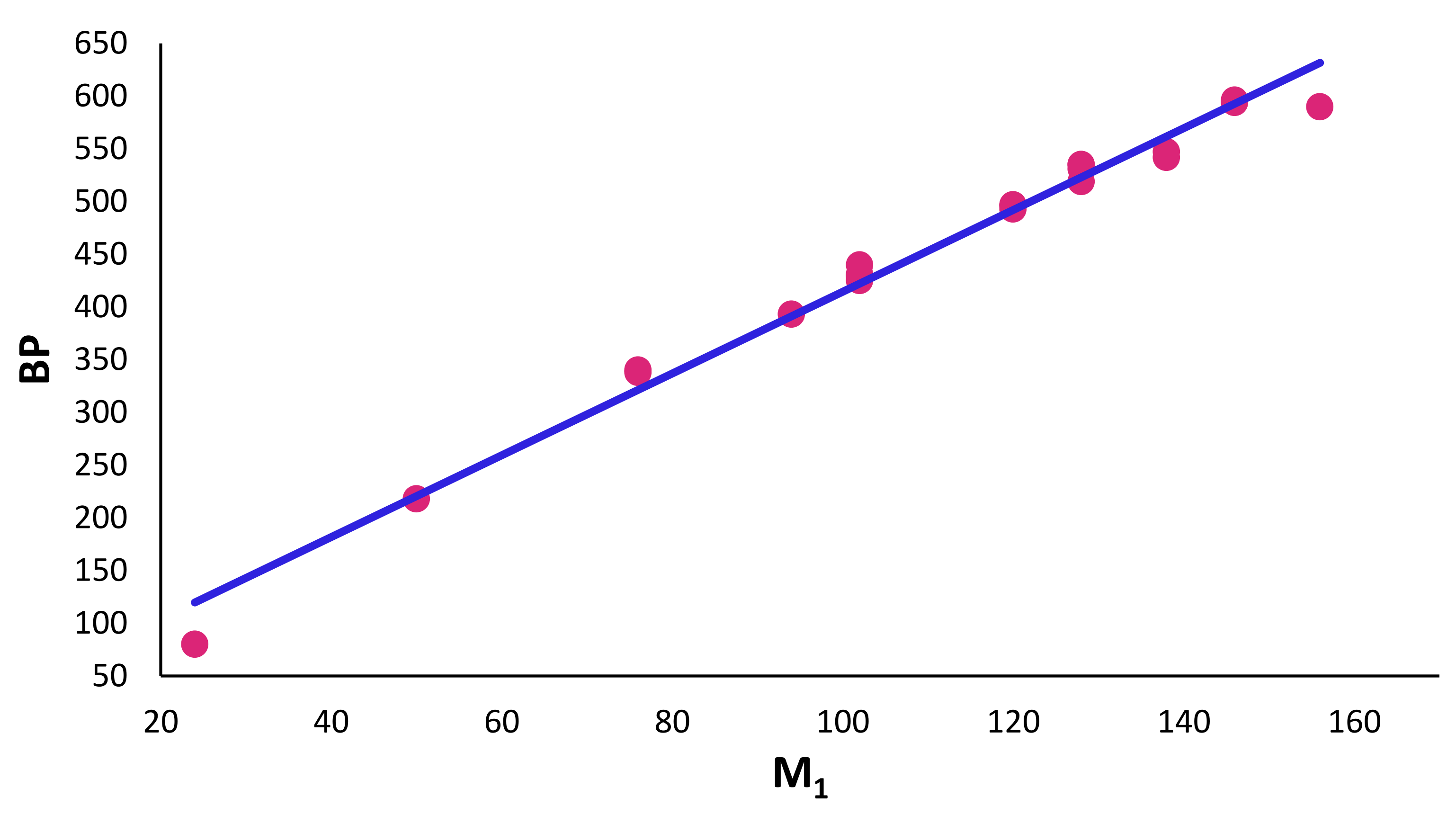
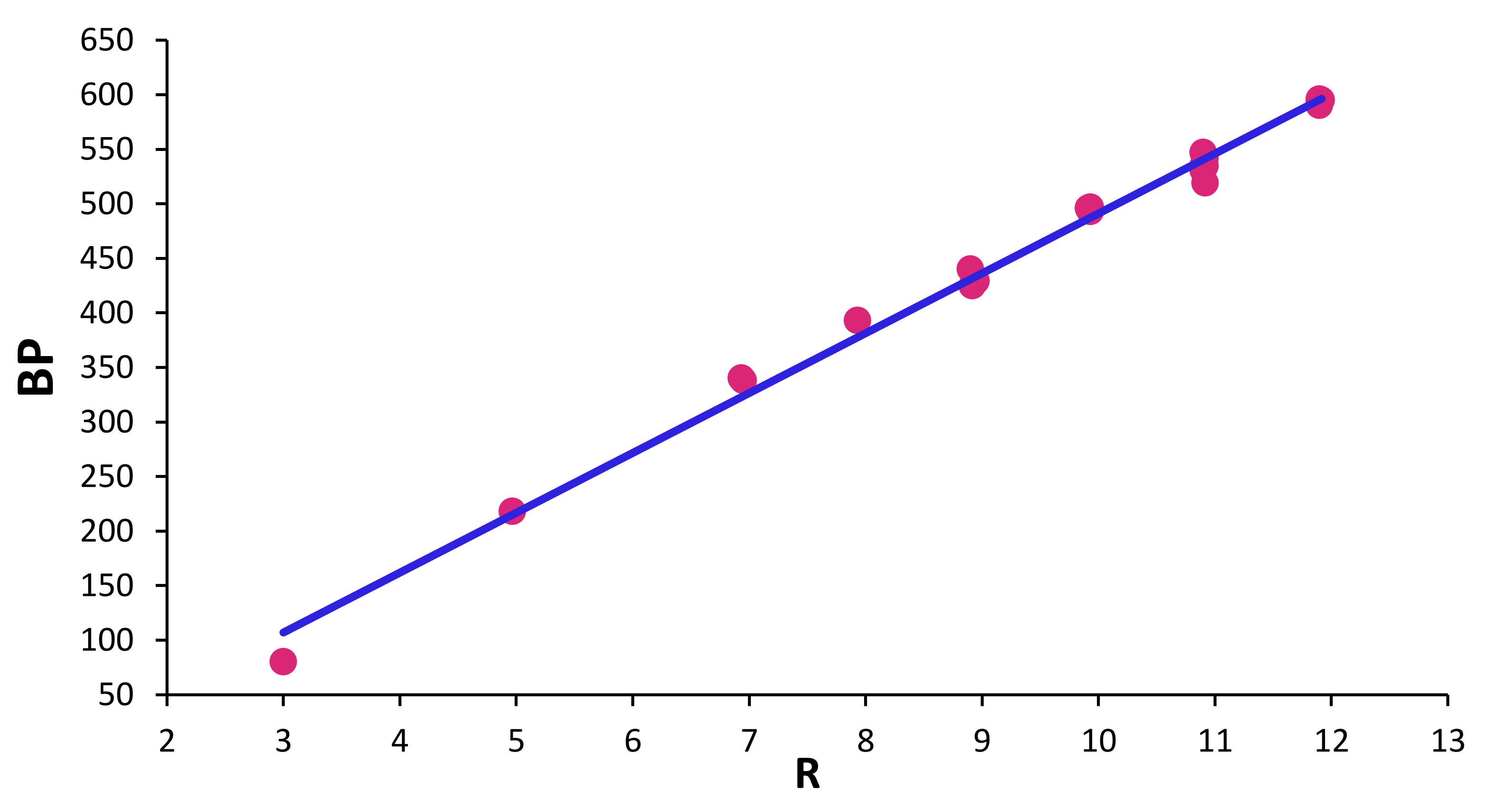
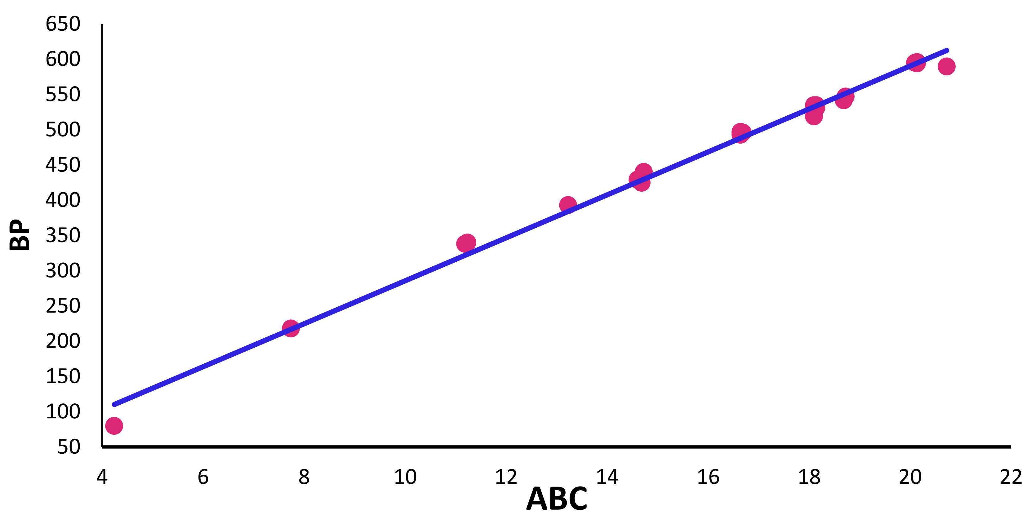
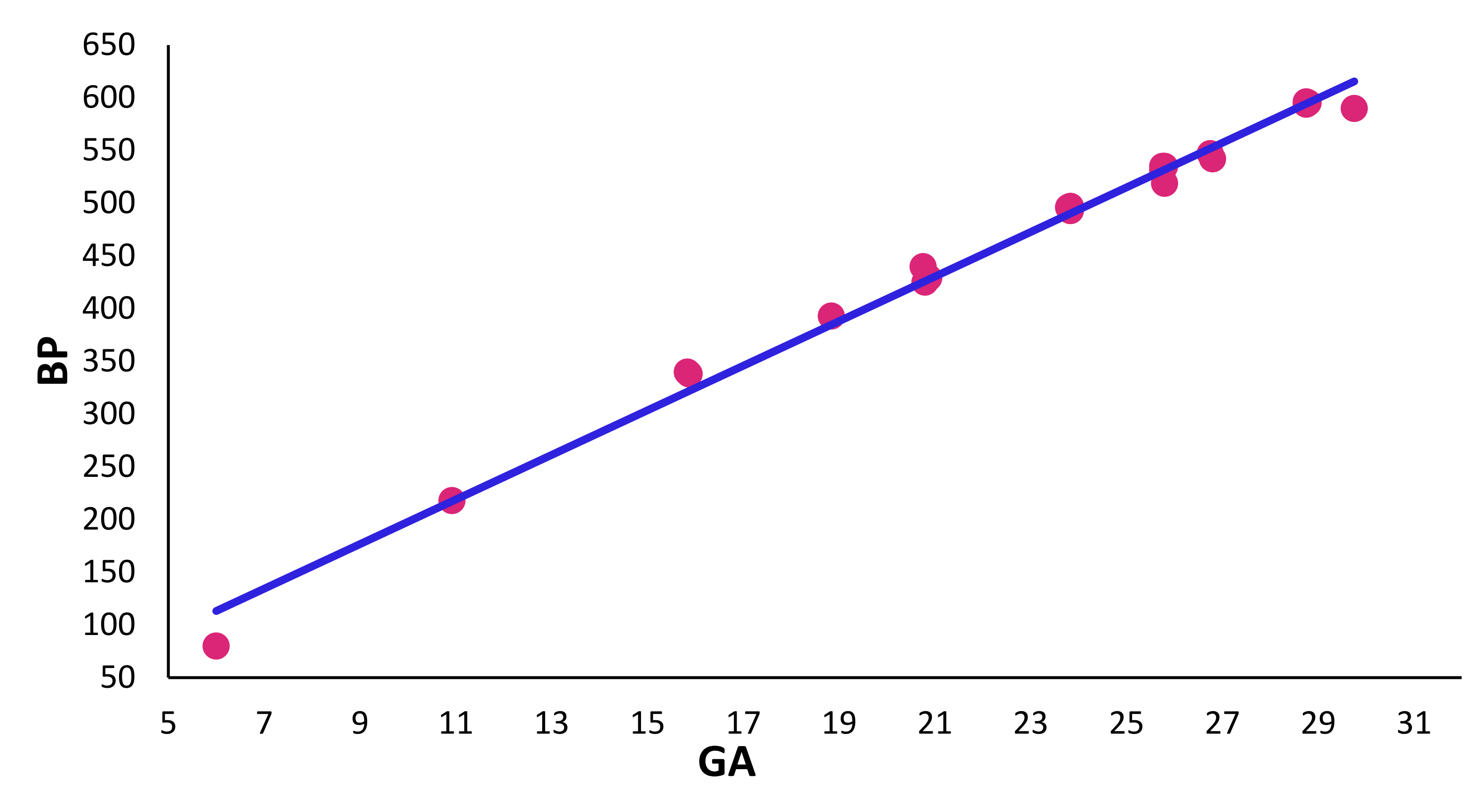
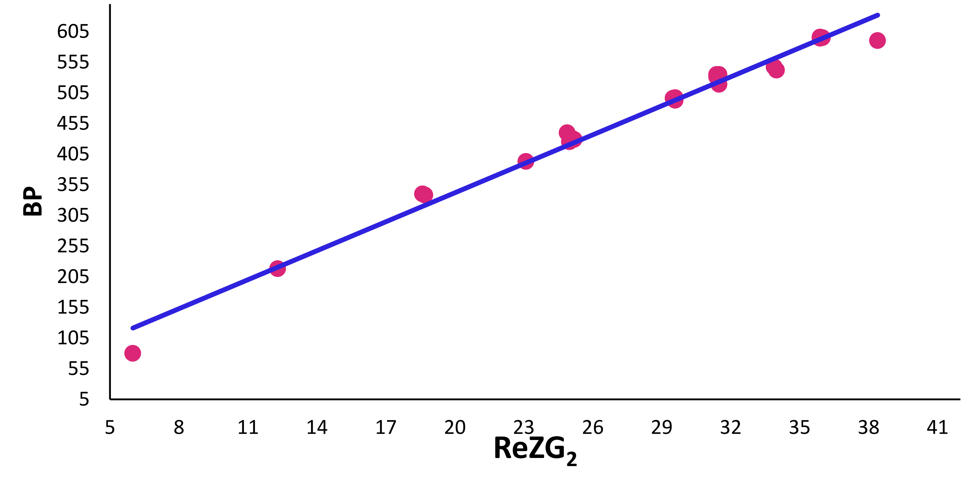
Figure 2: Graphical representation regression model between Boiling point and DB version of TIs.

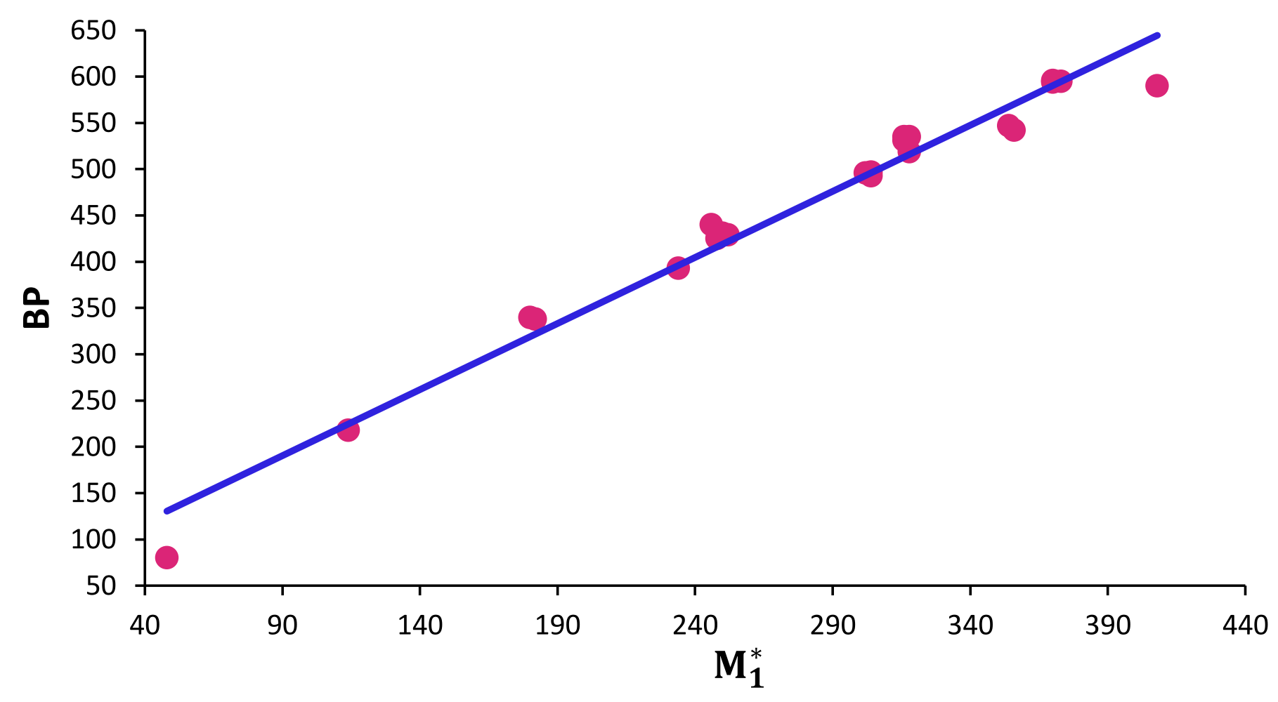
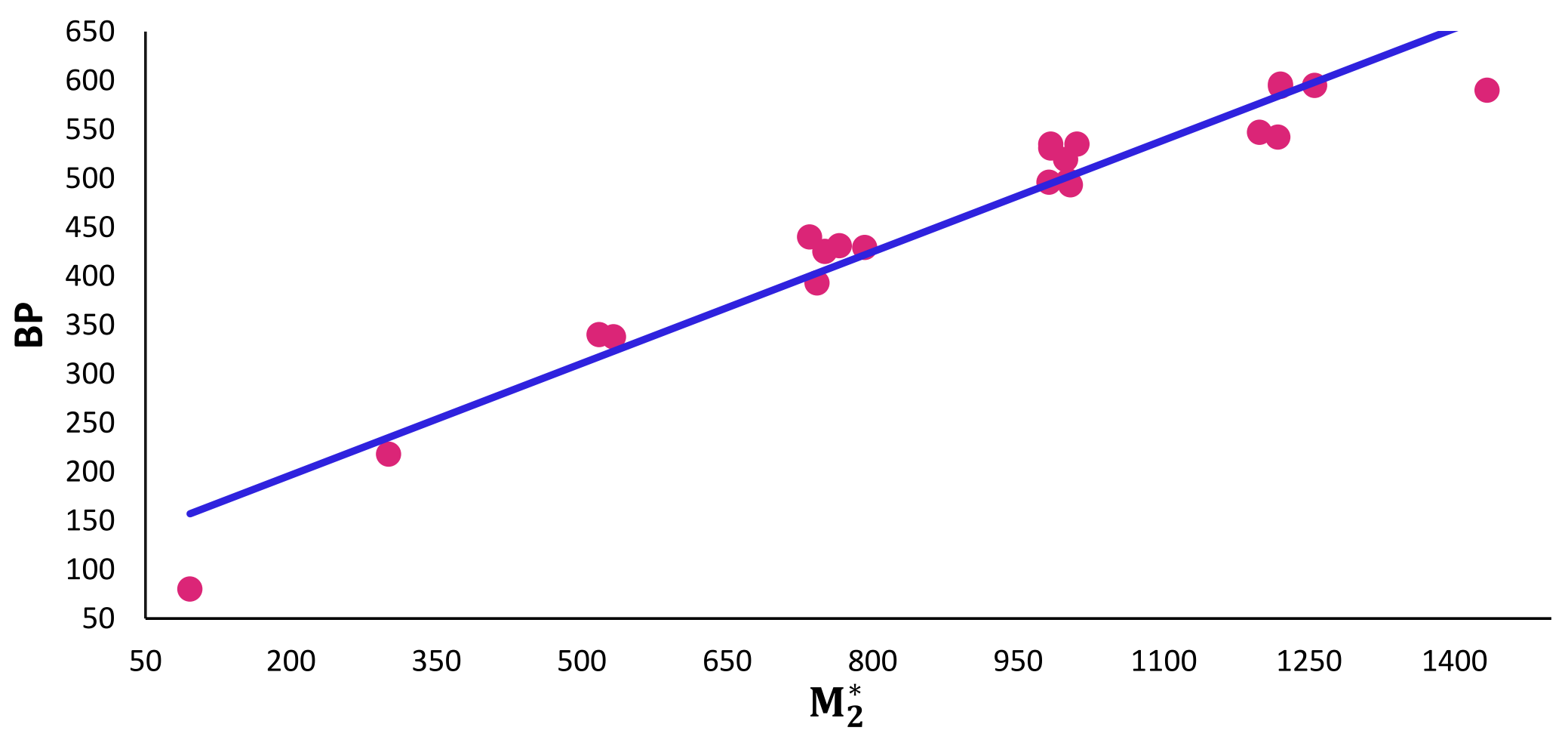
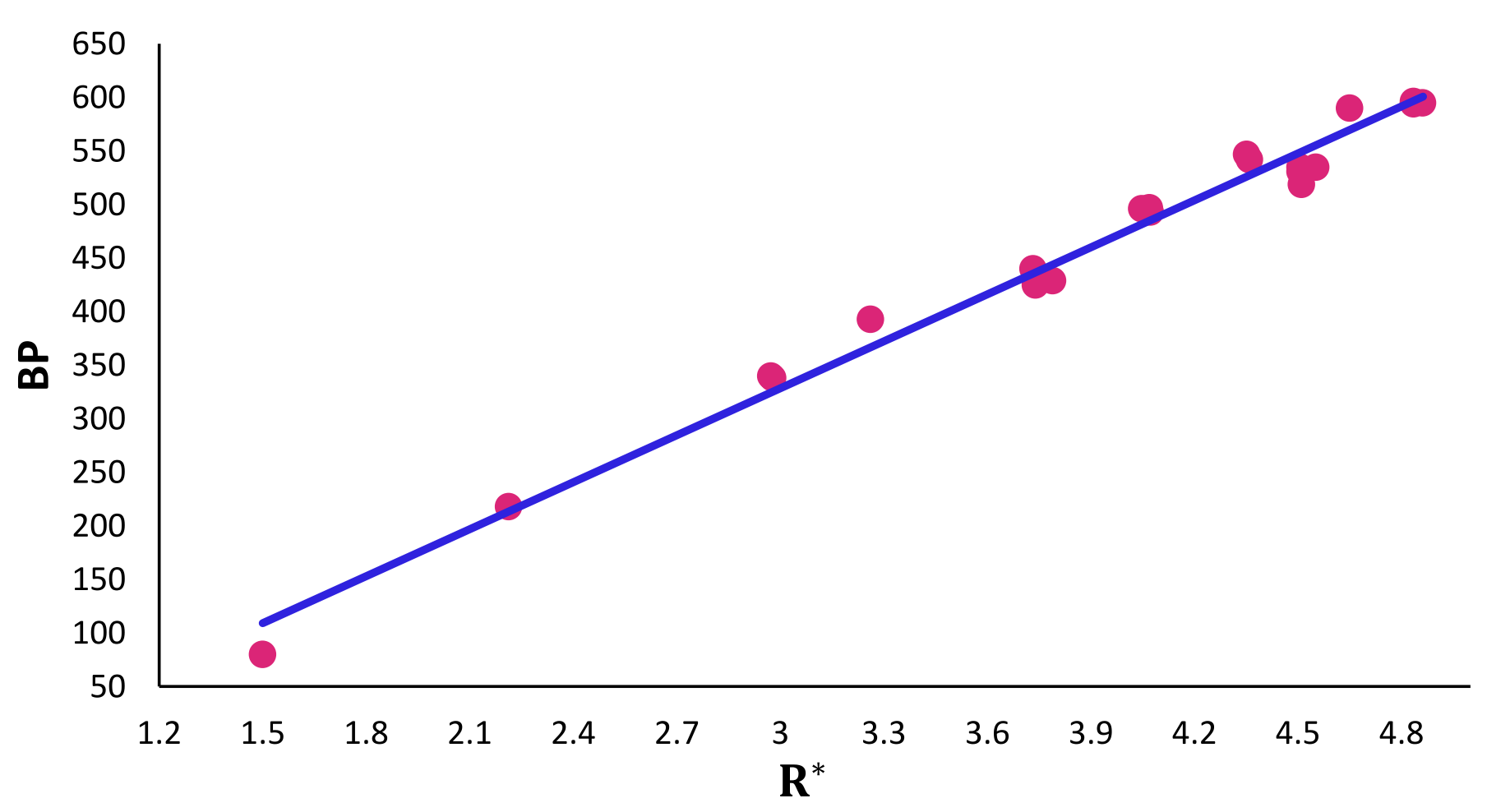
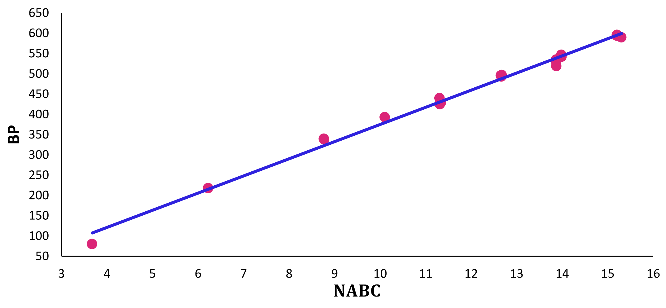
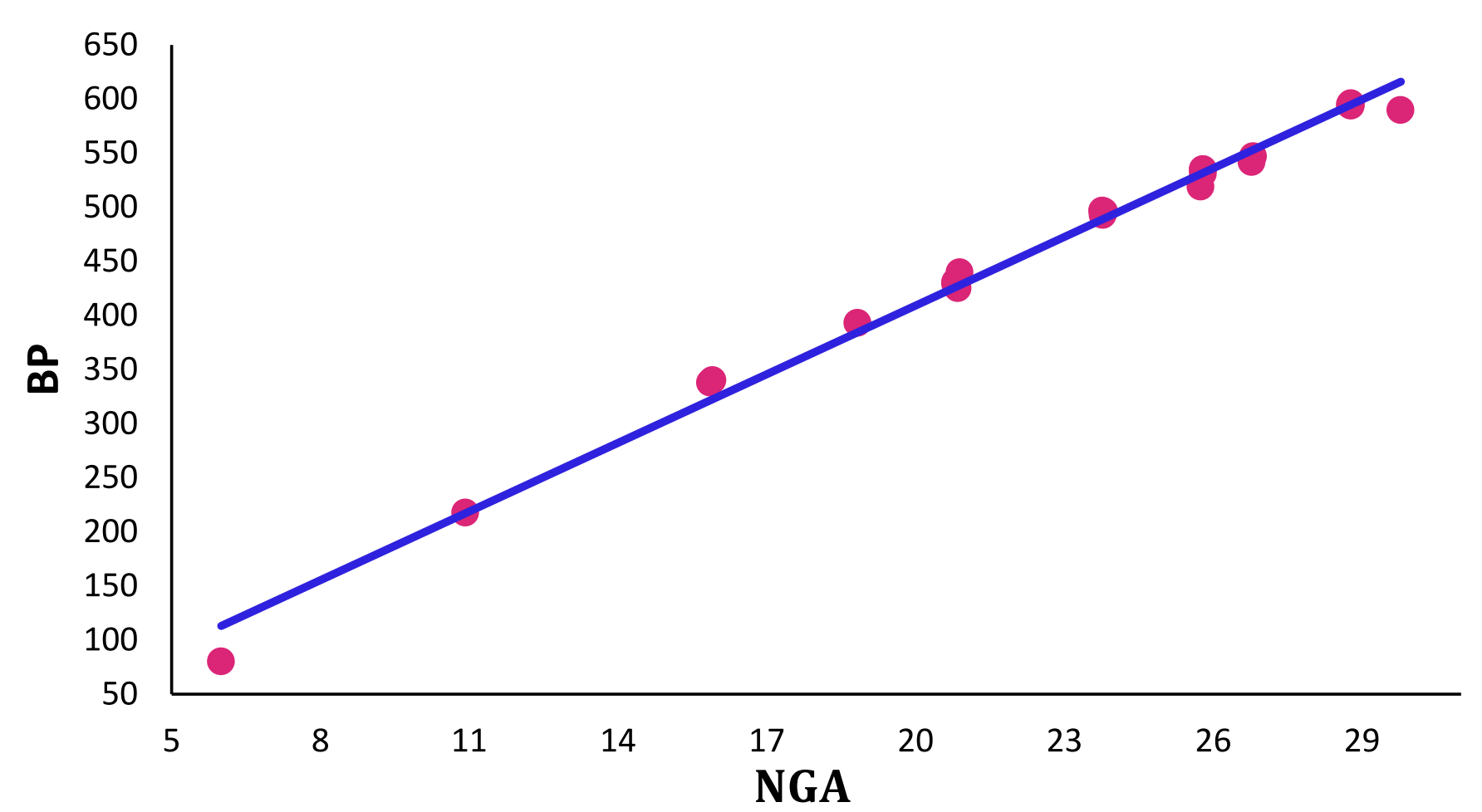
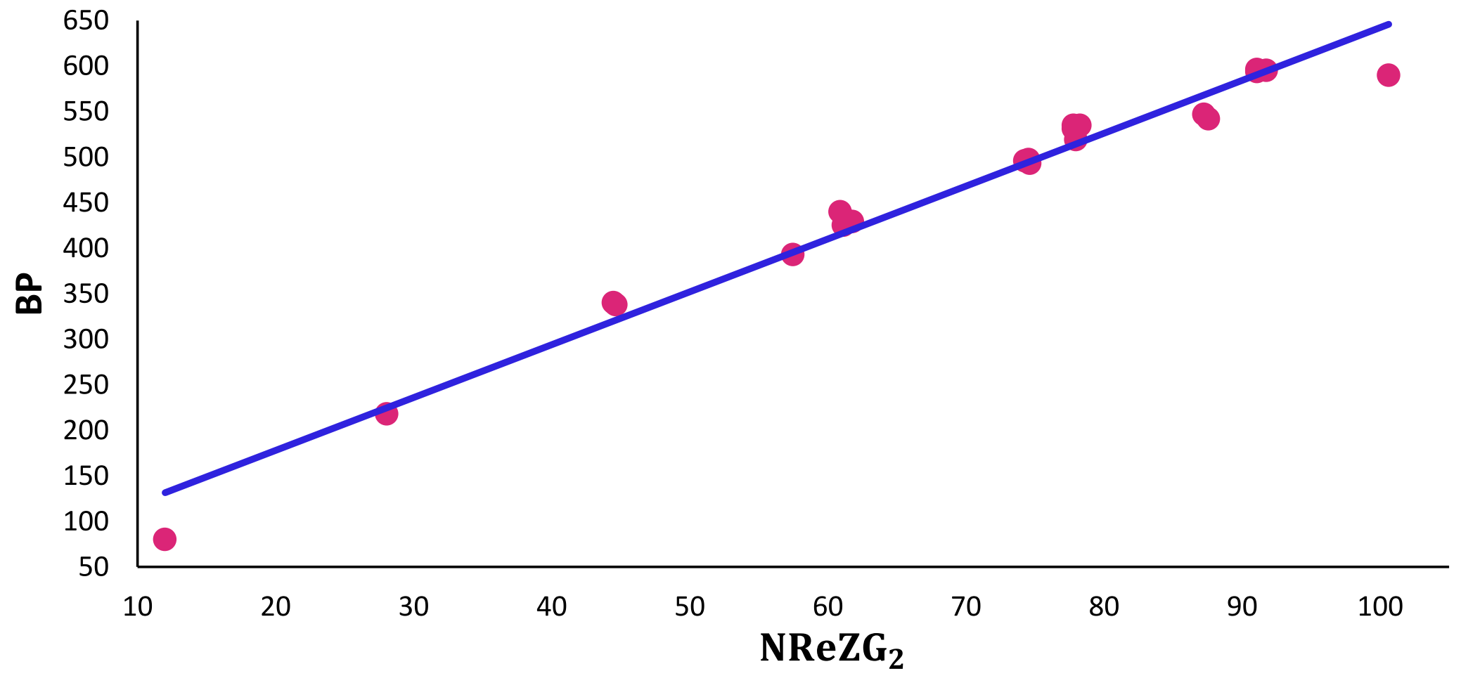
Figure 3: Graphical representation regression model between Boiling point and NDSB version of TIs.

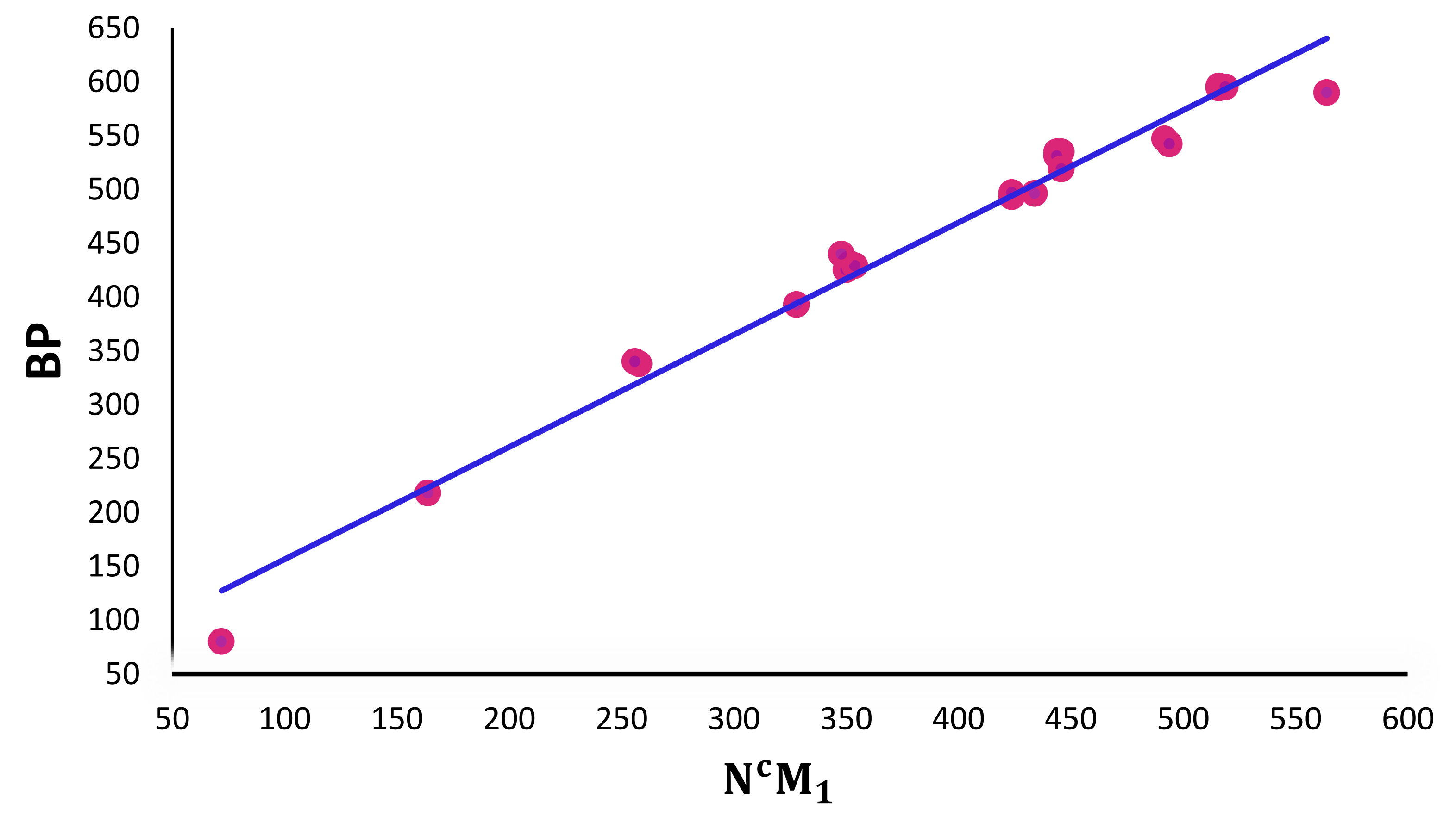
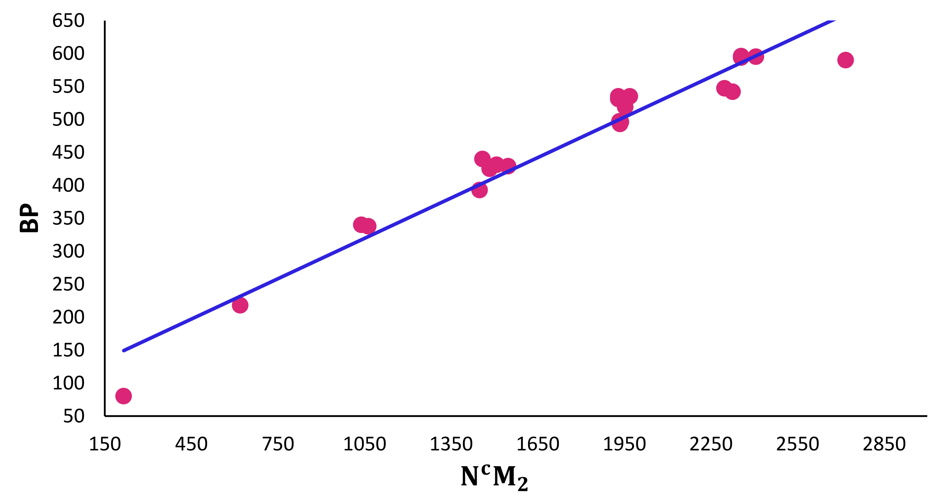
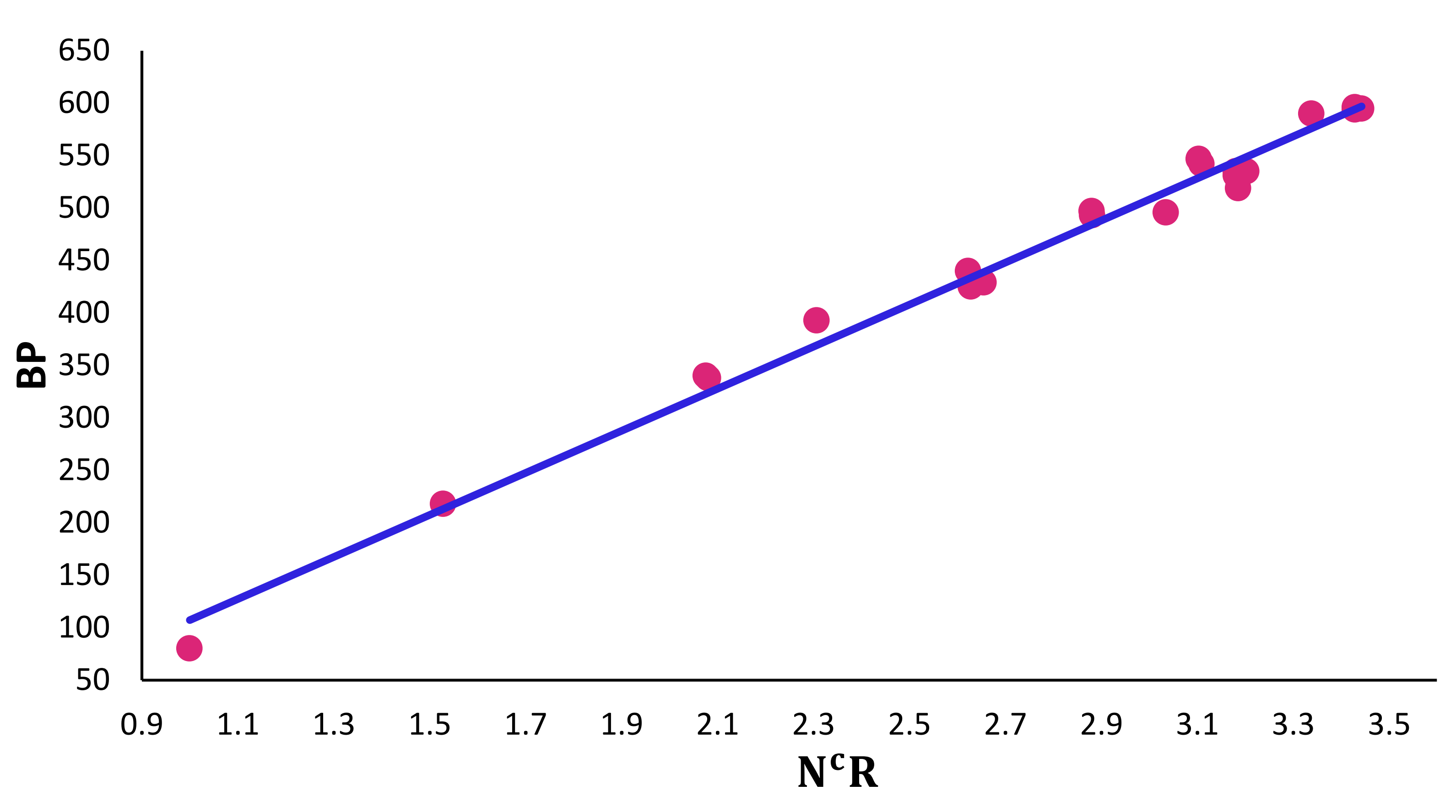
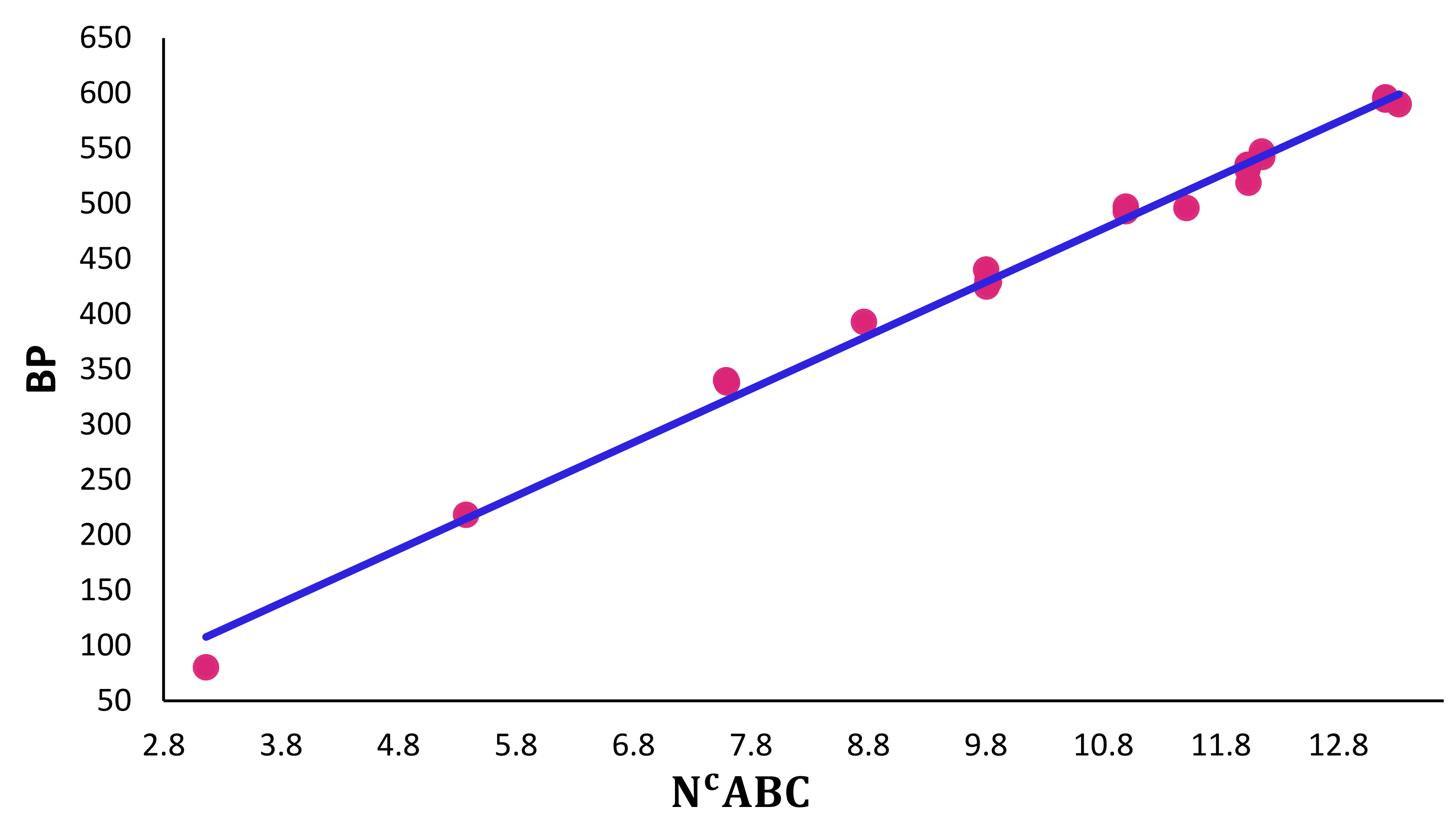
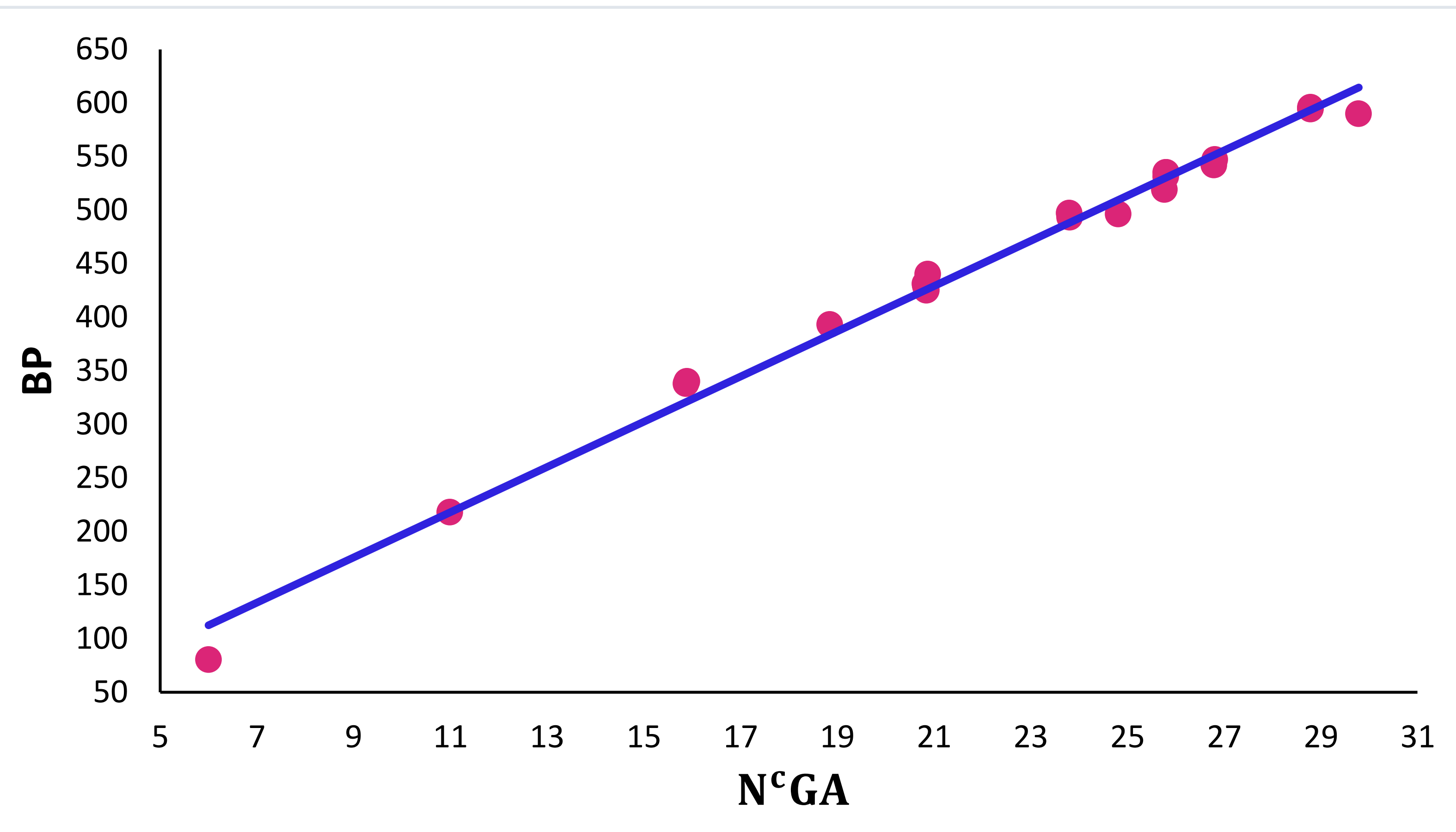
Figure 4: Graphical representation regression model between Boiling point and CNDSB version of TIs.

Table 5: The Significant regression model: Boiling point 22 lower PAHs on Degree-Based based form of TIs.

Descriptors	Regression Model	$R^{2}$	Correlation Coefficient (r)
$M_{1}$	$BP=3.8778M_{1}+26.629$	0.9845	0.99222
$M_{2}$	$BP=2.8577M_{2}+61.798$	0.9722	0.986002
$R$	$BP=54.87R-57.555$	0.9926	0.996293
$ABC$	$BP=30.467(ABC)-18.972$	0.9925	0.996243
$GA$	$BP=21.141(GA)-13.635$	0.9911	0.99554
$ReZG_{2}$	$BP=15.758(ReZG_{2})+26.863$	0.9834	0.991665

Table 6: The Significant regression model: Boiling point 22 lower PAHs on Neighborhood Degree Sum-Based form of TIs.

Descriptors	Regression Model	$R^{2}$	Correlation Coeffecient (r)
$M_{1}{}^{*}$	$BP=1.4281M_{1}^{*}+61.954$	0.9722	0.986002
$M_{2}{}^{*}$	$BP=0.3803M_{2}^{*}+120.62$	0.9362	0.967574
$R^{*}$	$BP=146.19R^{*}-110.17$	0.9837	0.991817
$NABC$	$BP=42.312(NABC)-48.038$	0.9933	0.996644
$NGA$	$BP=21.148(NGA)-13.878$	0.9913	0.99564
$NReZG_{2}$	$BP=5.8042(NReZG_{2})+61.859$	0.9717	0.985748

Table 7: The Significant regression model: Boiling point 22 lower PAHs on Closed Neighborhood Degree Sum-Based form of TIs.

Descriptor	Regression Model	$R^{2}$	Correlation Coeffecient (r)
$N^{c}M_{1}$	$BP=1.0427(N^{c}M_{1})+52.261$	0.9758	0.987826
$N^{c}M_{2}$	$BP=0.2041(N^{c}M_{2})+105.26$	0.9473	0.973293
$N^{c}R$	$BP=200.42(N^{c}R)-93.144$	0.9872	0.993579
$N^{c}ABC$	$BP=48.386(N^{c}ABC)-45.209$	0.9927	0.996343
$N^{c}GA$	$BP=21.102(N^{c}GA)-14.102$	0.9909	0.99544
$N^{c}ReZG_{2}$	$BP=4.2328(N^{c}ReZG_{2})+52.305$	0.9751	0.987472

Figure 5: Predictive potential comparison of DB, NDSB and CNDSB versions of considered TIs for BP.

5 Conclusion

In this manuscript we evaluate the predictive potential of six well known degree dependent TIs for three different versions with normal boiling point of 22 PAHs. We indicate that all considered TIs have excellent correlation with normal boiling point of considered group of molecules. In this article we develop QSPR analysis between three versions of six well known degree dependent TIs normal boiling points of 22 lower PAHs. The linear regression model shows, the Randic, Atom bond connectivity and Geometric Arithmetic Indices ($R,ABCandGA$) have the highest correlation Coefficient values with boiling point in all three versions. The DB version of considered TIs shows better results compared to the NDSB and CNDSB versions, the second best predictor version is CNDSB version.

References

- [1] Muhammad Shafii Abubakar, Kazeem Olalekan Aremu, and Maggie Aphane. Neighborhood versions of geometric–arithmetic and atom bond connectivity indices of some popular graphs and their properties. Axioms, 11(9):487, 2022.
- [2] Monjit Chamua, Jibonjyoti Buragohain, A Bharali, and Mohammad Essa Nazari. Predictive ability of neighborhood degree sum-based topological indices of polycyclic aromatic hydrocarbons. Journal of Molecular Structure, 1270:133904, 2022.
- [3] Matthias Dehmer, Frank Emmert-Streib, and Yongtang Shi. Quantitative graph theory: a new branch of graph theory and network science. Information Sciences, 418:575–580, 2017.
- [4] Emeric Deutsch and Sandi Klavžar. M-polynomial and degree-based topological indices. arXiv preprint arXiv:1407.1592, 2014.
- [5] Ernesto Estrada, Luis Torres, Lissette Rodriguez, and Ivan Gutman. An atom-bond connectivity index: modelling the enthalpy of formation of alkanes. Indian Journal of Chemistry -Section A (IJC-A), 37A:849–855, 1998.
- [6] Modjtaba Ghorbani and Mohammad A Hosseinzadeh. The third version of zagreb index. Discrete mathematics, algorithms and applications, 5(04):1350039, 2013.
- [7] Ivan Gutman and Kinkar Ch Das. The first zagreb index 30 years after. MATCH Commun. Math. Comput. Chem, 50(1):83–92, 2004.
- [8] Sakander Hayat, Suliman Khan, Asad Khan, and Muhammad Imran. Distance-based topological descriptors for measuring the -electronic energy of benzenoid hydrocarbons with applications to carbon nanotubes. Mathematical Methods in the Applied Sciences, 2020.
- [9] Sunilkumar M Hosamani, Bhagyashri B Kulkarni, Ratnamma G Boli, and Vijay M Gadag. Qspr analysis of certain graph theocratical matrices and their corresponding energy. Applied Mathematics and Nonlinear Sciences, 2(1):131–150, 2017.
- [10] Muhammad Yasir Hayat Malik, Muhammad Ahsan Binyamin, and Sakander Hayat. Correlation ability of degree-based topological indices for physicochemical properties of polycyclic aromatic hydrocarbons with applications. Polycyclic Aromatic Compounds, 42(9):6267–6281, 2022.
- [11] Sourav Mondal, Nilanjan De, and Anita Pal. On some new neighborhood degree-based indices for some oxide and silicate networks. J, 2(3):384–409, 2019.
- [12] Sourav Mondal, Muhammad Kamran Siddiqui, Nilanjan De, and Anita Pal. Neighborhood m-polynomial of crystallographic structures. Biointerface Res. Appl. Chem, 11(2):9372–9381, 2021.
- [13] R Pradeep Kumar, ND Soner, and MR Rajesh Kanna. Redefined zagreb, randic, harmonic, ga indices of graphene. International Journal of Mathematical Analysis, 11(10):493–502, 2017.
- [14] Milan Randic. Characterization of molecular branching. Journal of the American Chemical Society, 97(23):6609–6615, 1975.
- [15] Vignesh Ravi and Kalyani Desikan. Closed neighborhood degree sum-based topological descriptors of graphene structures. Biointerface Res. Appl. Chem, 12:7111–7124, 2022.
- [16] Damir Vukičević and Boris Furtula. Topological index based on the ratios of geometrical and arithmetical means of end-vertex degrees of edges. Journal of mathematical chemistry, 46:1369–1376, 2009.
- [17] Harry Wiener. Structural determination of paraffin boiling points. Journal of the American chemical society, 69(1):17–20, 1947.