Fast Variational Inference for Bayesian Factor Analysis in Single and Multi-Study Settings

Abstract

Factors models are routinely used to analyze high-dimensional data in both single-study and multi-study settings. Bayesian inference for such models relies on Markov Chain Monte Carlo (MCMC) methods which scale poorly as the number of studies, observations, or measured variables increase. To address this issue, we propose variational inference algorithms to approximate the posterior distribution of Bayesian latent factor models using the multiplicative gamma process shrinkage prior. The proposed algorithms provide fast approximate inference at a fraction of the time and memory of MCMC-based implementations while maintaining comparable accuracy in characterizing the data covariance matrix. We conduct extensive simulations to evaluate our proposed algorithms and show their utility in estimating the model for high-dimensional multi-study gene expression data in ovarian cancers. Overall, our proposed approaches enable more efficient and scalable inference for factor models, facilitating their use in high-dimensional settings. An R package VI-MSFA implementing our methods is available on GitHub (github.com/blhansen/VI-MSFA).

Keywords: Factor Analysis, Shrinkage prior, Variational Bayes, Multi-study

1 Introduction

Factor Analysis (FA) models are popular tools for providing low-dimensional data representations through latent factors. These factors are helpful to visualize, denoise and explain patterns of interest of the data, making FA models useful in several fields of application such as biology (Pournara and Wernisch,, 2007), finance (Ludvigson and Ng,, 2007), public policy (Samartsidis et al.,, 2020, 2021), and nutrition (Edefonti et al.,, 2012; Joo et al.,, 2018)—among many others.

In high-dimensional settings, FA models shrinking many latent factors’ components to zero are particularly helpful. These models allow focusing only on a small set of important variables, making the interpretation of the factors easier (Carvalho et al.,, 2008). Moreover, they can lead to more accurate parameter estimations compared to models that do not include shrinkage or sparsity (Avalos-Pacheco et al.,, 2022). In a Bayesian setting, many priors have been proposed to induce shrinkage or sparsity in the latent factors (e.g., Archambeau and Bach, (2008); Carvalho et al., (2008); Legramanti et al., (2020); Cadonna et al., (2020); Frühwirth-Schnatter, (2023)). A widely used one is the gamma process shrinkage prior (Bhattacharya and Dunson,, 2011; Durante,, 2017) that induces a shrinkage effect increasing with the number of factors. This prior adopts an adaptive approach for automatically choosing the latent dimension (i.e., the number of latent factors), facilitating posterior computation.

In a Bayesian context, inference on the posterior distribution of FA typically relies on Markov-Chain Monte Carlo (MCMC) algorithms (Lopes and West,, 2004), which scale poorly to high-dimensional settings (Rajaratnam and Sparks,, 2015). In addition, computing posterior expectations from MCMC can be computationally intensive. Specifically, many parameters are invariant to orthogonal transformations and must be post-processed before being averaged for inference, exacerbating time and memory needs. We refer to Papastamoulis and Ntzoufras, (2022) for examples of post-processing algorithms. In high-dimensional settings, MCMC for FA can also show poor mixing (Frühwirth-Schnatter et al.,, 2023), further increasing the difficulty of obtaining high-quality posterior inference without extensive computational resources.

While some alternatives to MCMC that seek the posterior mode via Expectation-Maximization (EM) algorithms have been developed for Bayesian FA (e.g., Ročková and George,, 2016), fast approximation of the posterior distribution that has the potential to scale inference in high-dimensional settings are still under-explored. Variational Bayes (VB) is one popular class of approximate Bayesian inference methods which has been successfully applied to approximate the posterior distribution of several models, such as logistic regression (Jaakkola and Jordan,, 1997; Durante and Rigon,, 2019), probit regression  (Fasano et al.,, 2022), latent Dirichlet allocation (Blei et al.,, 2017), and network factor models (Aliverti and Russo,, 2022), among others. VB has also been shown to scale Bayesian inference to high dimensional datasets for models closely related to FA. For example, Wang et al., (2020) consider item response theory models with latent factors, while Dang and Maestrini, (2022) proposes VB algorithms for structural equation models. However, VB for FA models with shrinkage priors is still under-explored, and to our knowledge, no VB implementations for FA with gamma process shrinkage priors exist. To address this issue and enable the practical use of FA in high-dimensional settings, we present two VB algorithms to approximate the posterior of this model and extend them to settings where multiple data from different sources are available.

There are many applications where data are collected from multiple sources or studies. These sources of information are then combined to produce more precise estimates and results that are robust to study-specific biases. For example, in biology, different microarray cancer studies can collect the same gene expression, measured in different platforms and/or with different late-stage patients. One standard approach to analyzing these multiple data is to stack them into a single dataset and perform FA (Wang et al.,, 2011). This approach can lead to misleading conclusions by ignoring potential study-to-study variability arising from both biological and technical sources (Garrett-Mayer et al.,, 2008). Therefore, statistical methods able to estimate concurrently common and study-specific signals should be used. Recent methods have been proposed to enable FA to integrate multiple sources of information in a single statistical model. These include perturbed factor analysis (Roy et al.,, 2021), Multi-study Factor Analysis (MSFA, De Vito et al.,, 2019, 2021), Multi-study Factor Regression (De Vito and Avalos-Pacheco,, 2023), and Bayesian combinatorial MSFA (Grabski et al.,, 2020).

In this paper, first, we present VB algorithms to conduct fast approximate inference for FA, and second, we extend these algorithms to a multi-study setting. We adopt the MSFA model, which decomposes the covariance matrix of the data in terms of common and study-specific latent factors and extend the gamma process shrinkage prior in this context (De Vito et al.,, 2019, 2021). Compared to current MCMC implementations, we show that VB approximations for FA and MSFA greatly reduce computation time while still providing accurate posterior inference.

The structure of this paper is as follows: Section 2 defines FA in a single study and describes VB estimation of the model parameters through Coordinate Ascent Variational Inference (CAVI) and Stochastic Variational Inference (SVI) algorithms; Section 3 generalizes these algorithms in a multi-study setting; Section 4 provides simulation studies benchmarking the performance of the proposed VB algorithms in comparison to previous MCMC based algorithms; Section 5 applies the proposed algorithms to a dataset containing gene expression values from $1,198$ patients with ovarian cancer across $4$ studies (Ganzfried et al.,, 2013); finally, Section 6 provides a brief discussion.

2 Factor Analysis

Let $\mathbf{x}_{i}=(x_{i1},\ldots,x_{iP})\in\mathbb{R}^{P}$ be a vector of $P$ centered observed variables for individual $i=1,\ldots,N$. FA assumes that $\mathbf{x}_{i}$ can be modelled as a function of $J\ll P$ latent factors or scores $\mathbf{l}_{i}\in\mathbb{R}^{J}$, and a corresponding factor loading matrix $\boldsymbol{\Lambda}\in\mathbb{R}^{P\times J}$ via

$$\mathbf{x}_{i}=\boldsymbol{\Lambda}\mathbf{l}_{i}+\mathbf{e}_{i},\hskip 14.22636pti=1,\ldots,N.$$ (1)

Both the factors $\{\mathbf{l}_{i}\}$ and the idiosyncratic errors $\{\mathbf{e}_{i}\}$ are assumed to be normally distributed, with $\mathbf{l}_{i}\sim\mathcal{N}_{J}(\boldsymbol{0},\boldsymbol{I}_{J})$, and $\mathbf{e}_{i}\sim\mathcal{N}_{P}(\boldsymbol{0},\boldsymbol{\Psi})$ where $\boldsymbol{\Psi}=\text{diag}\left(\psi_{1}^{2},\ldots,\psi_{P}^{2}\right)$. Factors $\{\mathbf{l}_{i}\}$ are assumed to be independent of errors $\{\mathbf{e}_{i}\}$, and the latent dimension $J\ll P$ is typically unknown. As a consequence, the observed covariance matrix, $\boldsymbol{\Sigma}=\mathrm{Cov}(\mathbf{x}_{i})$, can be expressed as $\boldsymbol{\Sigma}=\boldsymbol{\Lambda}\boldsymbol{\Lambda}^{\intercal}+\boldsymbol{\Psi}$. Given that $\boldsymbol{\Psi}$ is a diagonal matrix, the non-diagonal elements of $\boldsymbol{\Lambda}\boldsymbol{\Lambda}^{\intercal}$ represent the pairwise covariances of the $P$ variables, i.e., $\mathrm{Cov}(x_{ip},x_{iq})=\sum_{j=1}^{J}\lambda_{pj}\lambda_{qj}$ for $p\neq q$.

In the following, we will use $\mathbf{X}=\{\mathbf{x}_{i}\}$ to indicate the $N\times P$ data matrix used for the analysis.

2.1 Prior Specification

Following a Bayesian approach to inference for Model (1), we use the gamma process shrinkage prior of (Bhattacharya and Dunson,, 2011) for each element $\{\lambda_{pj}\}$ of the loading matrix $\boldsymbol{\Lambda}.$ Indicating with $\Gamma(a,b)$ a gamma distribution with mean $a/b$ and variance $a/b^{2}$, this prior can be expressed via:

$$\lambda_{pj}\mid\omega_{pj},\tau_{j}\sim\mathcal{N}(0,\omega_{pj}^{-1}\tau_{j}^{-1}),\quad p=1,\ldots,P,\quad j=1,\ldots\infty,$$

$$\omega_{pj}\sim\Gamma\left(\frac{\nu}{2},\frac{\nu}{2}\right),\quad\tau_{j}=\prod_{l=1}^{j}\delta_{l},\quad\delta_{1}\sim\Gamma(a_{1},1),\quad\delta_{l}\sim\Gamma(a_{2},1),\hskip 9.95863ptl\geq 2,$$ (2)

where $\delta_{l}\;(l=1,2,\dots)$ are independent, $\tau_{j}$ is a global shrinkage parameter for column $j$, and $\omega_{pj}$ is a local shrinkage parameter for element $p$ in column $j$.

In practice, prior (2) is truncated to a conservative upper bound $J^{*},$ smaller than $P$. We refer to Bhattacharya and Dunson, (2011) for more details on the choice of $J^{*}.$

Lastly, an inverse-gamma prior is placed on the diagonal entries of $\boldsymbol{\Psi}$, which is a common choice in FA (Lopes and West,, 2004; Ročková and George,, 2016):

$$\psi_{p}^{-2}\sim\Gamma(a^{\psi},b^{\psi}).$$ (3)

For simplicity, we denote all the model parameters with $\boldsymbol{\theta}=\left(\left\{\boldsymbol{\Lambda}_{p}\right\},\left\{\mathbf{l}_{i}\right\}\left\{\psi_{p}^{2}\right\},\left\{\omega_{pj}\right\},\left\{\delta_{l}\right\}\right)$ where $\boldsymbol{\Lambda}_{p}=(\lambda_{1p},\ldots,\lambda_{J^{*}p})$ is row $p$ of $\boldsymbol{\Lambda}$, and with $\pi(\boldsymbol{\theta})$ the prior (2)–(3).

2.2 Variational Inference for Factor Analysis

The goal of VB algorithms is to approximate the posterior distribution $p(\boldsymbol{\theta}|\mathbf{X})$, with a density $q^{*}(\boldsymbol{\theta})$ in a class $\mathcal{Q}$ (see  Blei et al., (2017) for further details). Specifically, the VB approximation of the posterior is defined as the distribution $q^{*}(\boldsymbol{\theta})\in\mathcal{Q}$ closest to $p(\boldsymbol{\theta}|\mathbf{X})$ in Kullback-Leibler (KL) divergence, satisfying the minimization:

$$\underset{q(\boldsymbol{\theta})\in\mathcal{Q}}{\arg\min}\left\{\text{KL}\left(q(\boldsymbol{\theta})\middle\|p(\boldsymbol{\theta}|\mathbf{X})\right)\right\}=\underset{q(\boldsymbol{\theta})\in\mathcal{Q}}{\arg\min}\left\{\int_{\boldsymbol{\Theta}}q(\boldsymbol{\theta})\log\frac{q(\boldsymbol{\theta})}{p(\boldsymbol{\theta}|\mathbf{X})}d\theta\right\},$$

or equivalently the maximization of the evidence based lower bound (ELBO):

$$\underset{q(\boldsymbol{\theta})\in\mathcal{Q}}{\arg\max}\left\{\text{ELBO}(q(\boldsymbol{\theta}))\right\}=\underset{q(\boldsymbol{\theta})\in\mathcal{Q}}{\arg\max}\left\{\mathbb{E}_{q(\boldsymbol{\theta})}[\log p(\boldsymbol{\theta},\mathbf{X})]-\mathbb{E}_{q(\boldsymbol{\theta})}[\log q(\boldsymbol{\theta})]\right\},$$ (4)

where $p(\boldsymbol{\theta},\mathbf{X})=p(\mathbf{X}|\boldsymbol{\theta})\pi(\boldsymbol{\theta})$ is the joint distribution of the data and $\boldsymbol{\theta},$ and the expectations are with respect to $q(\boldsymbol{\theta})$. A common approach to select $\mathcal{Q}$ is to use a mean-field variational family, $\mathcal{Q}^{\text{MF}}=\{q:q(\boldsymbol{\theta})=\prod_{m=1}^{M}q(\boldsymbol{\theta}_{m})\},$ that considers a partition of the parameters $\boldsymbol{\theta}$ into $M$ blocks, $(\boldsymbol{\theta}_{1},\ldots,\boldsymbol{\theta}_{M})$ and approximate the posterior with a product of $M$ independent density functions $q(\boldsymbol{\theta}_{m}),$ referred to as the variational factor for $\boldsymbol{\theta}_{m}$. When using $\mathcal{Q}^{\text{MF}},$ the variational factors $\{q^{*}(\boldsymbol{\theta}_{m})\}$ composing the VB approximation of the posterior can obtained from

$$q^{*}_{m}(\boldsymbol{\theta}_{m})\propto\exp\left(\mathbb{E}_{q(\boldsymbol{\theta}_{-m})}\left[\log(p(\boldsymbol{\theta}_{m}|\boldsymbol{\theta}_{-m},\mathbf{X})\right]\right),$$ (5)

where $\boldsymbol{\theta}_{-m}=(\boldsymbol{\theta}_{1},\ldots,\boldsymbol{\theta}_{m-1},\boldsymbol{\theta}_{m+1},\ldots,\boldsymbol{\theta}_{M})$ is the vector of parameters excluding the $m$-th one (Chapter §10, Bishop, (2006)).

When the conditional distribution $p(\boldsymbol{\theta}_{m}|\boldsymbol{\theta}_{-m},\mathbf{X})$ belongs to the exponential family, the corresponding optimal variational factor $q^{*}(\boldsymbol{\theta}_{m})$ also belongs to the same exponential family. Therefore, the maximization problem (4) reduces to learning the value of the parameters characterizing the distribution $q^{*}_{m}(\boldsymbol{\theta}_{m}).$ We will indicate these parameters as $\boldsymbol{\varphi}^{*}_{m}$ and the corresponding optimal variational factor as $q^{*}(\boldsymbol{\theta}_{m};\boldsymbol{\varphi}^{*}_{m}).$ Choosing $\mathcal{Q}^{\text{MF}}$ in such a way that $\{\pi(\boldsymbol{\theta}_{m})\}$ are conditionally conjugate prior for $\{\boldsymbol{\theta}_{m}\}$ enables the development of efficient algorithms such as the Coordinate-Ascent Variational Inference (CAVI) which learns $\boldsymbol{\varphi}^{*}$ by iteratively updating each parameter of $q^{*}(\boldsymbol{\theta}_{m};\boldsymbol{\varphi}^{*}_{m})$ conditional to the others variational factors until convergence is reached (Chapter § 10, Bishop, (2006)).

To implement CAVI for FA with priors (2)–(3), we propose the following mean-field variational family:

$$\begin{split}q(\boldsymbol{\theta};\boldsymbol{\varphi})=&\left[\prod_{l=1}^{J^{*}}q(\delta_{l};\alpha_{l}^{\delta},\beta_{l}^{\delta})\right]\left[\prod_{p=1}^{P}\prod_{j=1}^{J^{*}}q(\omega_{pj};\alpha_{pj}^{\omega},\beta_{pj}^{\omega})\right]\left[\prod_{i=1}^{N}q(\mathbf{l}_{i};\boldsymbol{\mu}_{i}^{l},\boldsymbol{\Sigma}_{i}^{l})\right]\times\\ &\left[\prod_{p=1}^{P}q(\boldsymbol{\Lambda}_{p};\boldsymbol{\mu}_{p}^{\Lambda},\boldsymbol{\Sigma}_{p}^{\Lambda})\right]\left[\prod_{p=1}^{P}q(\psi_{p}^{-2};\alpha_{p}^{\psi},\beta_{p}^{\psi})\right],\end{split}$$ (6)

with variational parameters $\boldsymbol{\varphi}=\left(\{\alpha_{l}^{\delta}\},\{\beta_{l}^{\delta}\},\{\alpha_{pj}^{\omega}\},\{\beta_{pj}^{\omega}\},\{\boldsymbol{\mu}_{i}^{l}\},\{\boldsymbol{\Sigma}_{i}^{l}\},\{\boldsymbol{\mu}_{p}^{\Lambda}\},\{\boldsymbol{\Sigma}_{p}^{\Lambda})\},\{\alpha_{p}^{\psi}\},\{\beta_{p}^{\psi}\}\right).$

The mean-field approximation in equation (6) factorizes the posterior distribution into conditionally conjugate elements, so maximizing the ELBO with respect to $q(\boldsymbol{\theta}_{m})$ leads to closed-form expressions for each variational parameter (Supplementary § D for details). All the steps to obtain the VB posterior approximation are detailed in Algorithm S1 (Supplementary § A).

An important aspect of CAVI is that each iteration requires optimizing the local parameters $\boldsymbol{\Sigma}^{l}_{i}$ and $\boldsymbol{\mu}^{l}_{i},$ relative to the scores $\mathbf{l}_{i}$ for $i=1,\ldots,N,$ which is computationally expensive in settings with large sample size. Thus, we propose a Stochastic Variational Inference (SVI) algorithm, which uses stochastic optimization to reduce the computational cost of each iteration (Hoffman et al.,, 2013). The key idea of this algorithm is to compute at each iteration the local parameters only for a small subset of available data and use this subset to approximate the remaining parameters common to all individuals, namely global parameters. In the following we use $\mathcal{M}^{\text{G}}\subset\{1,\ldots,M\}$ for the indices of the global parameters.

As a first step to illustrate the SVI algorithm, we reframe CAVI as a gradient-based optimization algorithm for the global parameters. Recall that the mean field approximation is constructed so that the optimal variational factors are distributions in the exponential family, i.e., a function of the natural parameters $\boldsymbol{\eta}\left(\mathbf{X},\boldsymbol{\theta}\right)$ (see Table S1 of Supplementary §A for details). With this parameterization, the derivative of the ELBO in equation (4) with respect to the natural parameters is (Hoffman et al.,, 2013):

$$\nabla ELBO(q(\boldsymbol{\theta}_{m}))=\mathbb{E}_{q(\boldsymbol{\theta}_{-m})}\left[\boldsymbol{\eta}\left(\mathbf{X},\boldsymbol{\theta}\right)\right]-\boldsymbol{\varphi}_{m}\quad\mbox{for}\quad m\in\mathcal{M}^{\text{G}}.$$ (7)

Equating the gradient (7) to $0,$ the solution of (4) can be written as $\boldsymbol{\varphi}_{m}=\mathbb{E}_{q(\boldsymbol{\theta}_{-m})}\left[\boldsymbol{\eta}\left(\mathbf{X},\boldsymbol{\theta}\right)\right]$.

The SVI replaces the gradient with an estimate much easier to compute. This is accomplished by selecting a batch-size parameter $b\in(0,1)$ and drawing a random sample of the data of dimension $\widetilde{N}=\lfloor b\times N\rfloor,$ at each iteration of the algorithm. Here $\lfloor x\rfloor,$ indicates the greatest integer less than or equal to $x.$ At iteration $t$, let $\mathcal{I}(t)\subseteq\{1,\ldots,N\}$ be the subset of sampled observations, and $\widetilde{\mathbf{X}}^{t}=\{\mathbf{x}_{i}\mbox{ for }i\in\mathcal{I}(t)\}$ the corresponding $\widetilde{N}\times P$ data matrix. SVI proceed by first updating the local parameters $\{\boldsymbol{\Sigma}^{l}_{i}\}$ and $\{\boldsymbol{\mu}^{l}_{i}\}$ for all $i\in\mathcal{I}(t),$ and then computing an approximated gradient for the global parameters via

$$\savestack{\tmpbox}{\stretchto{\scaleto{\scalerel*[\widthof{\nabla ELBO(q(\boldsymbol{\theta}_{m}))}]{\kern 0.1pt\mathchar 866\relax\kern 0.1pt}{\rule{0.0pt}{599.84122pt}}}{}}{2.4ex}}\stackon[-6.9pt]{\nabla ELBO(q(\boldsymbol{\theta}_{m}))}{\tmpbox}=\mathbb{E}_{q(\boldsymbol{\theta}_{-m})}\left[\boldsymbol{\eta}(\widetilde{\mathbf{X}}^{t},\boldsymbol{\theta})\right]-\boldsymbol{\varphi}_{m},\quad\mbox{for}\quad m\in\mathcal{M}^{\text{G}},$$ (8)

where the expectation $\mathbb{E}_{q(\boldsymbol{\theta}_{-m})}\left[\boldsymbol{\eta}(\widetilde{\mathbf{X}}^{t},\boldsymbol{\theta})\right]$ is computed giving weight $N/\widetilde{N}$ to each individual in $\mathcal{I}(t)$ (Hoffman et al.,, 2013). We call $\widehat{\boldsymbol{\varphi}}_{m}$ the solution of (8). At each iteration $t$ of the SVI algorithm, the update for the $\{\boldsymbol{\varphi}_{m}(t)\}$ of the global parameters is obtained as a weighted average of $\widehat{\boldsymbol{\varphi}}_{m}$ and $\boldsymbol{\varphi}_{m}{(t-1)}$ at the previous iteration:

$$\boldsymbol{\varphi}_{m}{(t)}=(1-\rho_{t})\boldsymbol{\varphi}_{m}{(t-1)}+\rho_{t}\widehat{\boldsymbol{\varphi}}_{m},\quad\mbox{for}\quad m\in\mathcal{M}^{\text{G}},$$ (9)

where $\rho_{t}$ is a step size parameter such that $\sum_{t}\rho_{t}\rightarrow\infty$ and $\sum_{t}\rho_{t}^{2}<\infty$ (Robbins and Monro,, 1951). The choice of $\rho_{t}$ can impact convergence. Step sizes which are too large may overweight estimated gradients and lead to unreliable estimates of variational parameter updates for some iterations, while step sizes which are too small may take many iterations to converge. A typical choice is to define $\rho_{t}=(t+\tau)^{-\kappa}$, where $\kappa\in(0.5,1]$ is the forgetting rate, which controls how quickly the variational parameters change across several iterations, and $\tau>0$ is the delay, which down-weights early iterations (Hoffman et al.,, 2013).

To implement SVI for FA, we reparameterize the global parameters in (6) in terms of the natural parameterization of the exponential family (Table S1 of Supplementary §A). The details are provided in Algorithm S2 (Supplementary §A).

3 Multi-study Factor Analysis

We extend the two algorithms presented in Section 2 to the setting where there are $S>1$ datasets measuring the same $P$ variables, using the MSFA Model (De Vito et al.,, 2021).

We indicate with $\mathbf{x}_{si}=(x_{si1},\ldots x_{siP})\in\mathbb{R}^{P}$ the vector of $P$ centered observed variables for individual $i=1,\ldots,N_{s}$ in study $s=1,\ldots,S$ and use the model

$$\mathbf{x}_{si}=\boldsymbol{\Phi}\mathbf{f}_{si}+\boldsymbol{\Lambda}_{s}\mathbf{l}_{si}+\mathbf{e}_{si}\quad i=1,\ldots,N_{s},\quad s=1,\ldots,S,$$ (10)

where $\mathbf{f}_{si}\sim\mathcal{N}_{K}(\boldsymbol{0},\boldsymbol{I}_{k})$ are the $K$-dimensional scores which correspond to the shared loading matrix $\boldsymbol{\Phi}\in\mathbb{R}^{P\times K},$ and $\mathbf{l}_{si}\sim\mathcal{N}_{J_{s}}(\boldsymbol{0},\boldsymbol{I}_{J_{s}})$ are the $J_{s}$-dimensional scores with study-specific loading matrices $\boldsymbol{\Lambda}_{s}\in\mathbb{R}^{P\times J_{s}}$. Finally, $\mathbf{e}_{is}\sim\mathcal{N}(\boldsymbol{0},\boldsymbol{\Psi}_{s})$ are study-specific idiosicratic errors with $\boldsymbol{\Psi}_{s}=\text{diag}\left(\psi_{s1}^{2},\ldots,\psi_{sp}^{2}\right)$. Model (10) can be seen as a generalization of Model (1) that incorporates shared latent components, $\boldsymbol{f}_{si}$ and $\boldsymbol{\Phi}$, and study-specific latent components, $\boldsymbol{l}_{si}$ and $\boldsymbol{\Lambda}_{s}$. The covariance matrices of each study $\boldsymbol{\Sigma}_{s}=\mathrm{Cov}(\mathbf{x}_{si})$ for $s=1,\ldots,S$ can be decomposed as $\boldsymbol{\Sigma}_{s}=\boldsymbol{\Phi}\boldsymbol{\Phi}^{\intercal}+\boldsymbol{\Lambda}_{s}\boldsymbol{\Lambda}_{s}^{\intercal}+\boldsymbol{\Psi}_{s}$. The terms $\boldsymbol{\Phi}\boldsymbol{\Phi}^{\intercal}$ and $\boldsymbol{\Lambda}_{s}\boldsymbol{\Lambda}_{s}^{\intercal}$ represent the portion of the covariance matrix that is attributable to the common factors and the study-specific factors, respectively. We refer to the $N_{s}\times P$ data matrix from study $s$ as $\mathbf{X}_{s}$.

3.1 Prior Specification

Following De Vito et al., (2021), we use the gamma process shrinkage prior (Bhattacharya and Dunson,, 2011) for both the study-specific and the shared loading matrix. The prior for each study-specific loading element $\lambda_{spj}$ is

$$\lambda_{spj}\mid\omega_{spj},\tau_{sj}\sim\mathcal{N}\left(0,\omega_{spj}^{-1}\tau_{sj}^{-1}\right),\quad s=1,\ldots,S\quad p=1,\ldots,P,\quad j=1,\ldots,\infty,$$

$$\omega_{spj}\sim\Gamma\left(\frac{\nu_{s}}{2},\frac{\nu_{s}}{2}\right),\quad\tau_{sj}=\prod_{l=1}^{j}\delta_{sl},\quad\delta_{s1}\sim\Gamma\left(a_{s1},1\right),\quad\delta_{sl}\sim\Gamma\left(a_{s2},1\right),\quad l\geq 2,$$ (11)

where $\delta_{sl}\;(l=1,2,\dots)$ are independent, $\tau_{sj}$ is the global shrinkage parameter for column $j$, and $\omega_{spj}$ is the local shrinkage for the element $p$ in column $j$. Similarly, the prior for each shared loading element $\boldsymbol{\phi}_{pk}$ is

$$\phi_{pk}\mid\omega_{pk},\tau_{k}\sim\mathcal{N}(0,\omega_{pk}^{-1}\tau_{k}^{-1}),\quad p=1,\ldots,P,\quad k=1,\ldots,\infty,$$

$$\omega_{pk}\sim\Gamma\left(\frac{\nu}{2},\frac{\nu}{2}\right),\quad\tau_{k}=\prod_{l=1}^{k}\delta_{l},\quad\delta_{1}\sim\Gamma(a_{1},1),\quad\delta_{l}\sim\Gamma(a_{2},1),\quad l\geq 2,$$ (12)

where $\delta_{l}\;(l=1,2,\dots)$ are independent, $\tau_{k}$ is the global shrinkage parameter for column $k$ and $\omega_{pk}$ is the local shrinkage parameter for element $p$ in column $k$.

These two priors introduce infinitely many factors for both the study-specific and the shared components (i.e., $J_{s}=\infty,$ for $s=1,\ldots,S$, and $K=\infty$). As detailed in Section (2), we truncate the latent dimensions using upper bounds $K^{*}$ and $J_{s}^{*},$ to all the studies. Finally, an inverse-gamma prior is used for the diagonal entries of $\boldsymbol{\Psi}_{s}$

$$\psi_{sp}^{-2}\sim\Gamma(a^{\psi},b^{\psi}).$$ (13)

We denote $\boldsymbol{\theta}=\left(\left\{\boldsymbol{\Phi}_{p}\right\},\left\{\boldsymbol{\Lambda}_{sp}\right\},\left\{\psi_{ps}^{2}\right\},\left\{\omega_{pk}\right\},\left\{\delta_{l}\right\},\left\{\omega_{spj}\right\},\left\{\delta_{sl}\right\}\right)$ as the vector of all model parameters, where $\boldsymbol{\Phi}_{p}$ is row $p$ of $\boldsymbol{\Phi}$ and $\boldsymbol{\Lambda}_{sp}$ is row $p$ of $\boldsymbol{\Lambda}_{s}$.

3.2 Variational Inference for Multi-Study Factor Analysis

The computational cost of Model (10) is larger than $S$ times the computational cost of Model (1) because we need to estimate both shared and study-specific parameters. Therefore, the benefit of fast VB approximation of the posterior is even higher than in the single study setting, especially if several high-dimensional studies are available for analysis. This is increasingly common in many applied settings, such as cancer genomics, where the expression levels of a large set of genes are measured across multiple cancer types.

To extend CAVI in a multi-study setting, we use the following mean field factorization

$$\begin{split}q(\boldsymbol{\theta};\boldsymbol{\varphi})&=\left[\prod_{l=1}^{K^{*}}q(\delta_{l};\alpha_{l}^{\delta},\beta_{l}^{\delta})\right]\left[\prod_{s=1}^{S}\prod_{l=1}^{J^{*}_{s}}q(\delta_{sl};\alpha_{sl}^{\delta},\beta_{sl}^{\delta})\right]\left[\prod_{p=1}^{P}\prod_{k=1}^{K^{*}}q(\omega_{pk};\alpha_{pk}^{\omega},\beta_{pk}^{\omega})]\right]\\ &\times\left[\prod_{s=1}^{S}\prod_{p=1}^{P}\prod_{j=1}^{J^{*}_{s}}q(\omega_{spj};\alpha_{spj}^{\omega},\beta_{spj}^{\omega})]\right]\left[\prod_{s=1}^{S}\prod_{i=1}^{N_{s}}q(\boldsymbol{f}_{si};\boldsymbol{\mu}_{si}^{f},\boldsymbol{\Sigma}_{si}^{f})]\right]\left[\prod_{s=1}^{S}\prod_{i=1}^{N_{s}}q(\mathbf{l}_{si};\boldsymbol{\mu}_{si}^{l},\boldsymbol{\Sigma}_{si}^{l})]\right]\\ &\times\left[\prod_{p=1}^{P}q(\boldsymbol{\Phi}_{p};\boldsymbol{\mu}_{p}^{\Phi},\boldsymbol{\Sigma}_{p}^{\Phi})]\right]\left[\prod_{s=1}^{S}\prod_{p=1}^{P}q(\boldsymbol{\Lambda}_{sp};\boldsymbol{\mu}_{sp}^{\Lambda},\boldsymbol{\Sigma}_{sp}^{\Lambda})]\right]\left[\prod_{s=1}^{S}\prod_{p=1}^{P}q(\psi_{sp}^{-2};\alpha_{sp}^{\psi},\beta_{sp}^{\psi})]\right]\end{split}$$ (14)

where $\boldsymbol{\Phi}_{p}$ is the $p^{th}$ row of $\boldsymbol{\Phi}$, $\boldsymbol{\Lambda}_{sp}$ is the $p^{th}$ row of $\boldsymbol{\Lambda}_{s}$, and

$$\begin{split}\boldsymbol{\varphi}=&\left(\{\alpha_{l}^{\delta}\},\{\beta_{l}^{\delta}\},\{\alpha_{sl}^{\delta}\},\{\beta_{sl}^{\delta}\},\{\alpha_{pk}^{\omega}\},\{\beta_{pk}^{\omega}\},\{\alpha_{spj}^{\omega}\},\{\beta_{spj}^{\omega}\},\right.\\ &\left.\{\boldsymbol{\mu}_{si}^{f}\},\{\boldsymbol{\Sigma}_{si}^{f}\},\{\boldsymbol{\mu}_{si}^{l}\},\{\boldsymbol{\Sigma}_{si}^{l}\},\{\boldsymbol{\mu}_{p}^{\Phi}\},\{\boldsymbol{\Sigma}_{p}^{\Phi}\},\{\boldsymbol{\mu}_{sp}^{\Lambda}\},\{\boldsymbol{\Sigma}_{sp}^{\Lambda}\},\{\alpha_{sp}^{\psi}\},\{\beta_{sp}^{\psi}\}\right)\end{split}$$

is the vector of variational parameters. Maximizing the ELBO with equation (5) leads to closed-form expressions for optimal variational parameters for each factor, conditional on the others (Supplementary §D for supporting calculations). Our implementation of CAVI for Bayesian MSFA is detailed in Algorithm S3 (Supplementary §A).

CAVI for MSFA requires computing both shared and study-specific scores for each observation in each study at each iteration. When $\{N_{s}\}$ are large, this can become very computationally demanding. Thus, we generalize the SVI algorithm described in Section 2 to the multi-study setting using the natural parameterization in Table S2 (Supplementary §A). The sub-sampling step of SVI is generalized to a multi-study setting by taking a sub-sample of size $\widetilde{N}_{s}=\lfloor b_{s}\times N_{s}\rfloor$ from each study. Our implementation of SVI for Bayesian MSFA is presented in Algorithm S4 (Supplementary §A).

4 Simulation Study

To assess the accuracy and computational performance of the CAVI and SVI algorithms for FA (Section 2) and MSFA (Section 3), we simulated different scenarios with varying numbers of subjects, variables, and studies. We compared the performance of the proposed algorithms (available at github.com/blhansen/VI-MSFA) with previously implemented Gibbs Sampler (GS) algorithms (available at github.com/rdevito/MSFA), in terms of: 1) computation time measured in seconds, 2) maximum RAM usage in megabytes (Mb), and, 3) estimation accuracy of $\boldsymbol{\Sigma}=\boldsymbol{\Lambda}\boldsymbol{\Lambda}^{\intercal}+\boldsymbol{\Psi}$ and $\boldsymbol{\Sigma}_{s}=\boldsymbol{\Phi}\boldsymbol{\Phi}^{\intercal}+\boldsymbol{\Lambda}_{s}\boldsymbol{\Lambda}_{s}^{\intercal}+\boldsymbol{\Psi}_{s}$ in the single and multi-study simulations, respectively. Computation time and RAM usage are monitored using the R package peakRAM (Quinn,, 2017), while estimation accuracy is evaluated using the RV coefficient between the true, $\boldsymbol{\Sigma}$ or $\boldsymbol{\Sigma_{s}}$, and the estimated covariance matrices, $\widehat{\boldsymbol{\Sigma}}$ or $\widehat{\boldsymbol{\Sigma_{s}}}$. The RV coefficient is a measure of similarity between two matrices varying between 0 and 1 defined as

$$\text{RV}(\mathbf{\boldsymbol{\Sigma}},\widehat{\boldsymbol{\Sigma}})=\frac{\operatorname{Tr}(\boldsymbol{\Sigma}\widehat{\boldsymbol{\Sigma}}^{\intercal}\widehat{\boldsymbol{\Sigma}}\boldsymbol{\Sigma}^{\intercal})}{\sqrt{\operatorname{Tr}(\boldsymbol{\Sigma}\boldsymbol{\Sigma}^{\intercal})^{2}\operatorname{Tr}(\widehat{\boldsymbol{\Sigma}}\widehat{\boldsymbol{\Sigma}}^{\intercal})^{2}}}.$$ (15)

An RV coefficient close to 1 (0) indicates strong similarity (dissimilarity) between the two matrices (Robert and Escoufier,, 1976).

For SVI Algorithms S2 and S4, we set the forgetting rate $\kappa$ and delay parameter $\tau$, which control the step-size schedule for $\rho_{t}$, to $\kappa=0.75$ and $\tau=1$. We must also specify the batch size parameters $b$, which control the number of points sampled at each iteration to estimate the gradient of the ELBO in Equation (8). The choice of batch size is non-trivial and consistently affects the accuracy and computational cost of the SVI algorithms. We refer to Tan, (2017) as recent work that considers the choice of batch size. To assess the effect of batch size on model performance in our settings, we consider batch sizes corresponding to $5\%,$ $20\%,$ and $50\%$ of the sample size, $b\in\{0.05,0.20,0.50\}$. For convenience, we will refer to SVI algorithms with these batch sizes as SVI-005, SVI-02, and SVI-05, respectively. Parameter initialization for CAVI and SVI is described in Supplementary §B. Convergence is monitored using the mean squared difference in parameters across iterations.

For GS, we draw $10,000$ posterior samples after a burn-in of $5,000$ and save in memory the values of the parameters every $5$ iterations, i.e., containing a total of $2,000$ samples. We then use these samples to compute the averages of $\boldsymbol{\Phi}\boldsymbol{\Phi}^{\intercal}$ and $\boldsymbol{\Lambda}_{s}\boldsymbol{\Lambda}_{s}^{\intercal}$ as point estimates of their respective posterior means. Note that $\boldsymbol{\Phi}\boldsymbol{\Phi}^{\intercal}$ and $\boldsymbol{\Lambda}_{s}\boldsymbol{\Lambda}_{s}^{\intercal}$ are identifiable functionals of the posterior of Model (10), therefore posterior means can be estimated directly by averaging the GS draws.

4.1 Single Study Simulations

We consider simulation scenarios for all combinations of $P=\{100,500,5000\}$ and $N=\{100,500,\allowbreak 1000\}$, generating the data from Model (1) with $J=4$ factors. For each scenario, we set each value of $\boldsymbol{\Lambda}$ to zero with probability $2/3$ or randomly generated it from an $\text{Uniform}(0,1)$ with probability $1/3.$ The values of $\boldsymbol{\Psi}$ are drawn from an $\text{Uniform}(0.1,1)$. Using the generated $\boldsymbol{\Sigma}=\boldsymbol{\Lambda}\boldsymbol{\Lambda}^{\intercal}+\boldsymbol{\Psi}$, we sample 50 datasets for each simulation scenario by taking $N$ draws from $\mathcal{N}_{p}(\boldsymbol{0},\boldsymbol{\Sigma})$. For each dataset, we estimate the posterior distribution of $\boldsymbol{\theta}$ with $J^{*}=5$ factors under priors (2)-(3) with hyperparameters $\nu=3$, $a_{1}=2.1$, $a_{2}=3.1$, $a^{\psi}=1$, and $b^{\psi}=0.3$ using GS, CAVI, and SVI previously described.

Table 1 reports, for each simulation scenario, the averages and standard deviations for the computation time, memory usage, and estimation accuracy. Comprehensive results are provided in Figures S1-S4 (Supplementary §C). Given the computational resources available, we found performing GS infeasible for the scenarios with $P=5,000$ and therefore, results are not reported (see caption of Table 1 for details).

As expected, CAVI required much less computational time than GS for every scenario. For example, in the scenario with $P=500$ and $N=1,000$, CAVI required, on average, $83$ seconds compared to $838$ for the GS. The average computation time of SVI was lower than CAVI in every simulation scenario with $N>100$, while in scenarios with $N=100$ and $P=100,500,$ SVI-005 required, on average, more computational time than CAVI. Note that in these scenarios, SVI-005 only uses $5$ observations to approximate the gradient in (8), requiring many iterations to converge. When the sample size increases, SVI is faster than CAVI. This is particularly evident for scenarios with larger $P$. For example, when $P=5,000$ and $N=1,000$ CAVI required on average approximately $32$ minutes compared to $12$, $6$ and $2$ minutes for SVI-05, SVI-02, and SVI-005 respectively. Additionally, SVI with small batch sizes scales better with increasing $N$. In the scenario with $P=5,000$, $N=100$, SVI-005, required an average of $20.7$ seconds. The computational time increases six times when $N=1,000$, while the computational time for SVI-02 and SVI-05 increases by 9 and 10 times, respectively.

Table 1: Average computational cost (in seconds), used RAM (in Mb), and estimation accuracy (RV coefficients) across 50 simulation replicates, mean(sd). Note: we were unable to run GS for scenarios with $P=5000$ due to memory limitations, as the allocated 128Gb of RAM for each algorithm was insufficient. This is indicated with ———- in the table.

		Time (Seconds)			Memory (Mb)			Estimation Accuracy $\left(\text{RV}(\widehat{\boldsymbol{\Sigma}},\boldsymbol{\Sigma})\right)$
method	N	P=100	P=500	P=5000	P=100	P=500	P=5000	P=100	P=500	P=5000
GS	100	136.01(2.12)	653.29(9.24)	———-	207.85(2.52)	4017.73(3.7)	———-	0.87(0.07)	0.73(0.11)	———-
CAVI	100	1.63(0.04)	8.9(0.12)	193.65(31.21)	23.27(0.62)	38.04(0.31)	555.6(69.65)	0.89(0.04)	0.78(0.04)	0.74(0.02)
SVI-005	100	4.4(0.06)	23.4(4.56)	20.7(0.31)	16.99(0.78)	36.05(1.64)	693.43(133.63)	0.83(0.06)	0.78(0.06)	0.59(0.05)
SVI-02	100	0.52(0.04)	2.92(0.07)	39.91(3.24)	20.32(1.27)	39.44(4.11)	656.76(83.49)	0.85(0.04)	0.75(0.04)	0.72(0.03)
SVI-05	100	0.88(0.04)	4.76(0.1)	75.81(10.85)	22.84(1.12)	38.14(0.3)	618.66(59.2)	0.88(0.04)	0.77(0.04)	0.73(0.02)
GS	500	159.73(2.82)	744.09(9.47)	———-	288.63(6.89)	4129(8.07)	———-	0.92(0.03)	0.93(0.03)	———-
CAVI	500	7.66(0.08)	43(0.5)	1111.03(86.01)	38.14(0.31)	49.77(1.6)	632.68(115.08)	0.96(0.01)	0.95(0.01)	0.93(0.01)
SVI-005	500	0.84(0.04)	4.36(0.06)	69.39(5.6)	24.49(0.81)	43.51(6.63)	617.6(125.65)	0.89(0.01)	0.9(0.01)	0.87(0.01)
SVI-02	500	1.83(0.05)	10.13(1.07)	170.14(8.42)	31.68(0.86)	49.6(2.47)	724.77(90.14)	0.93(0.01)	0.93(0.01)	0.91(0.01)
SVI-05	500	3.8(0.08)	20.09(0.2)	423.37(28.35)	38.12(0.14)	49.87(1.61)	651.02(109.93)	0.94(0.01)	0.94(0.01)	0.92(0.01)
GS	1000	186.49(2.26)	838.48(27.09)	———-	377(10.64)	4267.95(13.53)	———-	0.94(0.02)	0.97(0.02)	———-
CAVI	1000	15.45(0.27)	83.17(1.37)	1894.08(115.96)	37.74(0.31)	48.14(0.31)	662.41(126.27)	0.98(0.01)	0.97(0.01)	0.97(0.01)
SVI-005	1000	1.52(0.04)	8.15(0.12)	128.03(12.51)	33.65(0.64)	48.12(0.13)	720.5(154.13)	0.94(0.01)	0.95(0.01)	0.93(0.01)
SVI-02	1000	3.33(0.06)	18.34(1.45)	357.23(6.61)	37.74(0.31)	48.14(0.31)	885.96(122.91)	0.97(0.01)	0.96(0.01)	0.95(0.01)
SVI-05	1000	7.48(0.13)	37.55(0.6)	733.36(35.1)	37.74(0.31)	48.14(0.31)	669.48(117.82)	0.97(0.01)	0.97(0.01)	0.96(0.01)

In terms of memory usage, the computational burden of GS drastically increases with the number of variables. For example, GS required $377$ Mb of RAM memory on average when $N=1,000$ and $P=100$, and $4,267$ Mb when $P=500.$ In other words, when $P=500$ the memory requirements are approximately $11$ times the ones needed for $P=100$. In the same scenarios, the memory requirements of CAVI increase by approximately $1.3$ times, from $37$ Mb ($P=100$) to $48$ Mb ($P=500$). SVI algorithms have memory requirements that are very similar to CAVI.

In terms of accuracy, CAVI and SVI estimate $\boldsymbol{\Sigma}$ with comparable or greater accuracy to the posterior mean from GS in most scenarios. As expected, SVI performance deteriorates in scenarios with a small sample size and batch size. For example, in the scenario with $P=5,000$ and $N=100$, SVI-005 had an average RV of $0.59$ compared to $0.74$ of CAVI. However, the difference in performance between the two algorithms diminishes as the sample size increases. For example, when $P=5,000$ and $N=1,000$, SVI-005 has an average RV of $0.93$ compared to $0.97$ of CAVI.

4.2 Multi-study Simulations

Analogously to Section 4.1, we assess the performance of the proposed VI algorithms in the multi-study setting. We consider simulation scenarios with $S=\{5,10\}$, $P\in\{100,500,5000\}$ and $N_{s}=\{100,500,1000\}$, generating the data from Model (10) with $K=4$ common factors and $J_{s}=4,s=1,\ldots,S$ study-specific factors. For each scenario, factor matrices $\boldsymbol{\Phi}$ and $\boldsymbol{\Lambda}_{s}$ are randomly generated setting each values to $0$ with probability $2/3$ or drawing from an $\text{Uniform}(0,1)$ with probability $1/3,$ while the values of $\boldsymbol{\Psi}_{s},s=1,\ldots,S$ are generated from an $\text{Uniform}(0.1,1).$ Using the generated $\boldsymbol{\Sigma}_{s}$, we sample $50\times S$ by taking $N_{s}$ draws from $\mathcal{N}(\boldsymbol{0},\boldsymbol{\Phi}\boldsymbol{\Phi}^{\intercal}+\boldsymbol{\Lambda}_{s}\boldsymbol{\Lambda}_{s}^{\intercal}+\boldsymbol{\Psi}_{s})$ for each study. We estimate the posterior distribution of $\boldsymbol{\theta}$ with $K^{*}=5$, $J_{s}^{*}=5$ under priors (11)-(13) with hyperparameters $\nu=3=\nu_{s}=3$, $a_{1}=a_{s1}=2.1$, $a_{2}=a_{s2}=3.1$, $a^{\psi}=1$, and $b^{\psi}=0.3$ using the multi-study versions of GS, CAVI, and SVI, described in Section 4. As we found in the single study simulations, we were unable to run the scenarios with $P=5,000$ for GS within the limited amount of memory available.

Table 2: Average computation time in seconds, mean(sd), for 50 multi-study simulation replicates. Note: we were unable to run GS for scenarios with $P=5000$ due to memory limitations, as the allocated 128Gb of RAM for each algorithm was insufficient. This is indicated with ———- in the table.

		S = 5			S = 10
method	N_s	P= 100	P=500	P=5000	P=100	P=500	P=5000
GS	100	1731.81(79.41)	7202.42(299.4)	———-	2909.89(202.01)	13685.49(344.14)	———-
CAVI	100	13.89(0.16)	69.9(0.65)	697.79(6.09)	27.49(0.27)	139.36(1.24)	1401.71(16.29)
SVI-005	100	4.44(0.31)	16.21(0.15)	180.43(1.9)	8.21(0.48)	30.53(1.36)	347.75(5.76)
SVI-02	100	5.87(0.09)	29.38(0.27)	302.95(5.19)	11.94(0.15)	57.25(0.64)	598.81(7.89)
SVI-05	100	10.91(0.13)	54.34(0.53)	673.59(17.66)	21.69(0.21)	126.08(1.98)	1249.23(81.52)
GS	500	2007.95(88.86)	9592.4(436.29)	———-	3836.87(170.46)	18216.42(753.08)	———-
CAVI	500	65.58(0.67)	337.83(3.57)	3388.28(43.33)	129.99(1.86)	699.48(7.14)	6882.88(141.35)
SVI-005	500	36.27(1.59)	81.83(2.59)	551.53(8.29)	53.81(1.92)	125.72(1.07)	1080.07(14.22)
SVI-02	500	43.54(2.16)	112.96(1.36)	1147.65(17.58)	63.59(2.17)	222.09(1.88)	2319.4(29.8)
SVI-05	500	50.88(3.69)	259.15(16.9)	2622.91(139.1)	92.8(1.11)	543.75(27.8)	5209.9(267.22)
GS	1000	2723.13(151.94)	11959.9(155.65)	———-	5080.1(193.06)	23502.28(1052.9)	———-
CAVI	1000	132.42(1.53)	700.22(6.95)	6819.3(135.85)	261.7(5.93)	1356.8(34.54)	13834.76(457.48)
SVI-005	1000	97.22(6.04)	203.83(6.01)	1022(31.56)	147.04(5.04)	337.12(7.07)	2045.03(71.37)
SVI-02	1000	121.12(7.04)	251.76(14.49)	2242.47(43.76)	177.35(8.68)	434.82(5.74)	4611.19(73.49)
SVI-05	1000	141.7(8.27)	516.37(15.9)	5091.47(323.48)	223.6(15.52)	1107.08(21.68)	10256.13(281.85)

Table 2 reports the average computational times (refer to Figure S5, Supplementary §C for comprehensive results). CAVI and SVI required much less time on average than GS in every simulation scenario.

For example, in the scenario with $S=10$, $P=500$, and $N_{s}=1,000$, CAVI required an average of approximately $23$ minutes to converge while GS took more than $7$ hours, making CAVI about 18 times faster than GS. In the same scenario, SVI algorithms were even faster, taking approximately $19,$ $7,$ and $6$ minutes on average for SVI-05, SVI-02 and SVI-005 respectively, making SVI algorithms between 23 to 76 times faster than GS.

Table 3: Average peak RAM usage in Mb, mean(sd), for 50 multi-study simulation replicates. Note: we were unable to run GS for scenarios with $P=5000$ due to memory limitations, as the allocated 128Gb of RAM for each algorithm was insufficient. This is indicated with ———- in the table.

		S = 5			S = 10
method	N_s	P= 100	P=500	P=5000	P=100	P=500	P=5000
GS	100	124.75(3.44)	523.74(18.34)	———-	183.27(2.95)	868.86(14.05)	———-
CAVI	100	35.15(1.09)	48.99(1.5)	797.77(111.56)	37.35(0.35)	62.35(1.75)	906.55(53.12)
SVI-005	100	34.98(0.88)	48.89(1.48)	759.64(63.26)	37.35(0.35)	62.67(0.52)	863.54(86.26)
SVI-02	100	34.98(0.88)	49.06(0.3)	699.2(57.98)	37.35(0.35)	62.67(0.52)	865.35(100.53)
SVI-05	100	34.98(0.88)	49.16(0.42)	684.01(8.97)	37.35(0.35)	62.67(0.52)	843.03(119.51)
GS	500	209.02(17.85)	740.74(42.34)	———-	275.11(13.34)	1180.84(67.13)	———-
CAVI	500	36.35(0.34)	99.7(2.86)	997.45(142.89)	63.63(1.92)	140.49(1.36)	1422.85(139.16)
SVI-005	500	36.35(0.34)	99.7(2.86)	1009.33(136.62)	58.37(7.63)	139.41(1.51)	1351.75(100.59)
SVI-02	500	49.3(2.45)	99.7(2.86)	1027.07(151.17)	60.71(6.45)	143.04(0.99)	1390.39(146.67)
SVI-05	500	49.58(1.57)	99.7(2.86)	955.19(120.17)	62.24(4.73)	143.04(0.99)	1351.11(114.97)
GS	1000	212.93(19.84)	1011.04(63.94)	———-	295.55(22.99)	1542.8(193.03)	———-
CAVI	1000	48.05(0.34)	142.44(1)	1354.05(112.44)	70.05(0.34)	268.75(14.87)	2447.45(107.4)
SVI-005	1000	62.22(5.16)	141.43(10)	1342.89(100.68)	88.37(7.35)	265.75(18.49)	2500.8(90.85)
SVI-02	1000	61.57(5.86)	142.54(0.99)	1332.46(102.73)	87.94(7.78)	259.57(26.23)	2423.05(38.01)
SVI-05	1000	59(7.52)	133.45(15.8)	1362.02(107.35)	70.05(0.35)	262.9(6.21)	2444.2(72.12)

Table 3 reports the average memory usage (refer to Figure S6, Supplementary §C, for the comprehensive results). The proposed algorithms require much less memory than GS in all the scenarios. For example, GS required 3.5 times as much memory as CAVI in the setting with $S=5$, $N_{s}=100$, $P=100$ (125 Mb compared to 35 Mb), while in the setting with $S=10$, $N_{s}=1000$, $P=500$ GS required about 6 times more memory than CAVI (1542 Mb compared to 269 Mb). In all scenarios, CAVI and SVI have comparable memory requirements.

Table 4: Average estimation accuracy, reported as RV between estimated $\boldsymbol{\Sigma}_{s}=\boldsymbol{\Phi}\boldsymbol{\Phi}^{\intercal}+\boldsymbol{\Lambda}_{s}{\boldsymbol{\Lambda}_{s}}^{\intercal}+\boldsymbol{\Psi}_{s}$ and the simulation truth, mean(sd), for 50 multi-study simulation replicates. Note: we were unable to run GS for scenarios with $P=5000$ due to memory limitations, as the allocated 128Gb of RAM for each algorithm was insufficient. This is indicated with ———- in the table.

		S = 5			S = 10
method	N_s	P= 100	P=500	P=5000	P=100	P=500	P=5000
GS	100	0.93(0.02)	0.91(0.04)	———-	0.91(0.03)	0.92(0.04)	———-
CAVI	100	0.86(0.05)	0.86(0.03)	0.86(0.02)	0.84(0.04)	0.89(0.02)	0.86(0.02)
SVI-005	100	0.72(0.06)	0.68(0.05)	0.68(0.05)	0.68(0.05)	0.68(0.05)	0.68(0.04)
SVI-02	100	0.84(0.05)	0.84(0.03)	0.85(0.02)	0.8(0.04)	0.87(0.03)	0.85(0.02)
SVI-05	100	0.85(0.05)	0.86(0.03)	0.86(0.02)	0.81(0.04)	0.89(0.02)	0.87(0.02)
GS	500	0.98(0.01)	0.98(0.01)	———-	0.99(0.01)	0.99(0.01)	———-
CAVI	500	0.86(0.05)	0.92(0.01)	0.96(0.02)	0.94(0.01)	0.96(0.01)	0.96(0.01)
SVI-005	500	0.87(0.04)	0.91(0.01)	0.94(0.02)	0.93(0.01)	0.94(0.01)	0.94(0.01)
SVI-02	500	0.85(0.04)	0.92(0.01)	0.95(0.02)	0.92(0.02)	0.95(0.01)	0.96(0.01)
SVI-05	500	0.84(0.04)	0.92(0.01)	0.96(0.02)	0.92(0.02)	0.95(0.01)	0.96(0.01)
GS	1000	0.99(0.01)	0.99(0.01)	———-	0.99(0.01)	0.99(0.01)	———-
CAVI	1000	0.91(0.05)	0.95(0.02)	0.97(0.02)	0.94(0.02)	0.96(0.02)	0.98(0.01)
SVI-005	1000	0.92(0.04)	0.94(0.02)	0.96(0.02)	0.94(0.02)	0.95(0.02)	0.97(0.01)
SVI-02	1000	0.91(0.04)	0.94(0.02)	0.97(0.02)	0.92(0.02)	0.95(0.02)	0.97(0.01)
SVI-05	1000	0.9(0.05)	0.94(0.02)	0.97(0.02)	0.92(0.03)	0.96(0.02)	0.98(0.01)

Table 4 reports the averages and standard deviations of the RV coefficients between estimated $\boldsymbol{\Sigma}_{s}$ and the simulation truth. We refer to Figure S7 for comprehensive results for $\boldsymbol{\Sigma}_{s}$ and Figures S8 and S9 for the RV coefficients of $\boldsymbol{\Phi}$ and $\boldsymbol{\Lambda}_{s}$, respectively. As before, CAVI estimates $\boldsymbol{\Sigma}_{s}$ with comparable accuracy to GS. In scenarios where the number of observations is small, CAVI is less accurate than GS. For example, when $P=100$ and $N_{s}=100$, CAVI has an average RV of $0.86$ compared to $0.93$ of the GS. When the sample size increases, the average RV of CAVI is closer to GS. For example, when $P=500$ and $N_{s}=1,000$ CAVI as an average RV of $0.95$ compared to $0.99$ of the GS. When both the sample and batch size are small, the SVI algorithms can present poor performance. When $N_{s}$ is low, the performance of SVI with a small batch size can be inferior to CAVI, especially in high dimensional settings. For example, with $P=5,000$ and $N_{s}=100$, the average RV of SVI-005 was $0.68$ while CAVI had an average RV of $0.86$. The difference between SVI and CAVI is much smaller with larger batch sizes—the RVs were comparable to CAVI for SVI-02 and SVI-05 across all 18 simulation scenarios. When $N_{s}>100$, SVI-005 presented an accuracy comparable with CAVI for all the considered values of $P$ and $S$.

5 Case Study: Ovarian Cancer Gene Expression Data

We apply the proposed algorithms to four high-dimensional datasets containing microarray gene expression data available in the R package curatedOvarianData 1.36 (Ganzfried et al.,, 2013). The curated ovarian cancer studies contain $N_{s}=\left\{578,285,195,140\right\}$ patient observations. We selected genes with observed variances in the highest 15% in at least one study, resulting in a final set of $P=3643$ genes. Each dataset was centered and scaled before analysis.

We start by evaluating the ability of MSFA to predict out-of-sample $\mathbf{x}_{si}$ compared to alternative FA models in a 10-fold cross-validation . In particular, we consider three models: 1) A MSFA as described in Section 3; 2) A FA fitted on a dataset stacking all the $S=4$ studies (Stacked FA); 3) Independent FA models for each study (Independent FA). For the MSFA model 1) we set $K^{*}=10$ and $J^{*}_{s}=10,$ and use CAVI and SVI (with $b_{s}=0.5$ for $s=1,\ldots,4$). For FA in 2) and 3), we set $J^{*}=10$ using CAVI and SVI ($b=0.5$). It is important to emphasize that fitting these models with GS would have required more than 128Gb of RAM to be allocated (the limit set in Section 4); therefore, this was considered not feasible.

Predictions are computed as follows:

$$\textit{MSFA:}\;\widehat{\mathbf{x}}_{si}=\widehat{\boldsymbol{\Phi}}\widehat{\mathbf{f}}_{si}+\widehat{\boldsymbol{\Lambda}}_{s}\widehat{\mathbf{l}}_{si}\qquad\qquad\textit{Stacked FA:}\;\widehat{\mathbf{x}}_{si}=\widehat{\boldsymbol{\Phi}}\widehat{\mathbf{f}}_{si}\qquad\qquad\textit{Independent FA:}\;\widehat{\mathbf{x}}_{si}=\widehat{\boldsymbol{\Lambda}}_{s}\widehat{\mathbf{l}}_{si}.$$

Factor scores for out-of-sample observations are derived by adapting Bartlett’s method (Bartlett,, 1937) for MSFA:

$$\widehat{\mathbf{f}}_{si} =\left((\widehat{\boldsymbol{\Phi}},\widehat{\boldsymbol{\Lambda}}_{s})^{\intercal}\widehat{\boldsymbol{\Psi}}_{s}^{-1}(\widehat{\boldsymbol{\Phi}},\widehat{\boldsymbol{\Lambda}}_{s})\right)^{-1}\widehat{\boldsymbol{\Phi}}^{\intercal}\widehat{\boldsymbol{\Psi}}_{s}^{-1}\mathbf{x}_{si},$$ (16)

$$\widehat{\mathbf{l}}_{si} =\left((\widehat{\boldsymbol{\Phi}},\widehat{\boldsymbol{\Lambda}}_{s})^{\intercal}\widehat{\boldsymbol{\Psi}}_{s}^{-1}(\widehat{\boldsymbol{\Phi}},\widehat{\boldsymbol{\Lambda}}_{s})\right)^{-1}\widehat{\boldsymbol{\Lambda}}_{s}^{\intercal}\widehat{\boldsymbol{\Psi}}_{s}^{-1}\mathbf{x}_{si},$$ (17)

where $(\widehat{\boldsymbol{\Phi}},\widehat{\boldsymbol{\Lambda}}_{s})$ is obtained by stacking the common and study-specific factor loading matrices, and $\widehat{\boldsymbol{\Phi}}$ and $\widehat{\boldsymbol{\Lambda}}_{s}$, $\widehat{\Psi}_{s}$ denote the posterior mode of the respective VI approximation.

Table 5: Computation time (in minutes) and MSE, reported as mean(sd), across the 10 cross-validation folds. Relative MSE is the average MSE divided by the average MSE of MSFA fitted using CAVI (the best-performing algorithm). For independent FA the time include fitting $S=4$ serially.

Method	Time (minutes)	MSE	Relative MSE
MSFA (CAVI)	11.06(0.24)	2296(53)	1
MSFA (SVI)	8.83(0.24)	2315(52)	1.01
Independent FA (CAVI)	14.41(0.16)	2435(55)	1.06
Independent FA (SVI)	6.77(0.036)	2447(50)	1.06
Stacked FA (CAVI)	13.58(0.19)	2531(52)	1.10
Stacked FA (SVI)	6.07(0.093)	2527(53)	1.10

Results of the 10-fold cross-validation are reported in Table 5. Despite the high dimensionality of the dataset, the proposed VB algorithms were able to fit the MSFA model with an average computation time of approximately 11 minutes for CAVI and 9 minutes for SVI. Also, the two considered FA approaches were computed in a small amount of time, approximately 14 minutes for CAVI and 7 minutes for SVI. In terms of MSE, CAVI and SVI share a similar performance, decreasing the MSE of 10% compared to Stacked FA and 6% compared to Independent FA.

We then estimated the common covariance $\boldsymbol{\widehat{\Sigma}}_{\Phi}=\widehat{\boldsymbol{\Phi}}\widehat{\boldsymbol{\Phi}}^{\intercal}$ with MSFA via CAVI and represented it via a gene co-expression network (Figure 1). A gene co-expression network is an undirected graph where the nodes correspond to genes, and the edges correspond to the degree of co-expression between genes. The number of connections between genes is visualized in the plot by the size of each node, i.e., the bigger, the more connected. We identified two different and important clusters. The first cluster contains genes associated with the immune system and cell signaling, such as CD53 (Dunlock,, 2020), LAPTM5 (Glowacka et al.,, 2012), PTPRC (Hermiston et al.,, 2003), TYROBP (Lanier et al.,, 1998), C1QA/C1QB (Liang et al.,, 2022). Also, in the first cluster, some genes play a crucial role in cancer, such as SAMSN1 (Yan et al.,, 2013) and FCER1G (Yang et al.,, 2023). The second network includes genes such as FBN1 known to promote metastasis in ovarian cancer (Wang et al.,, 2015), and SERPINF1 crucial to the prognosis of cancer (Zhang et al.,, 2022).

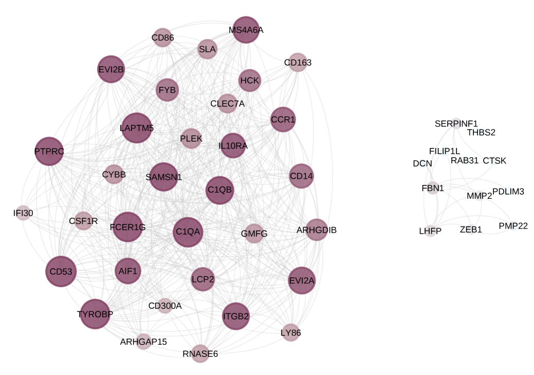
Figure 1: Common gene co-expression network estimated via $\widehat{\boldsymbol{\Phi}}\widehat{\boldsymbol{\Phi}}^{\intercal}$ across the four ovarian cancer studies. The network is obtained using Gephi via the Fruchterman-Reingold algorithm  (Bastian et al.,, 2009). We include edges if $\widehat{\boldsymbol{\Phi}}\widehat{\boldsymbol{\Phi}}^{\intercal}\geq|0.5|$, and exclude from the figure nodes with no edges. The figure includes 92 nodes and 851 edges.

The gene network in Figure 1 reveals the ability of the MSFA to discover common signal pathways across different studies, critically helpful in ovarian cancer and generalizable to new context areas. These results further show the ability of the proposed VB algorithms to provide reliable results in a short computation time.

6 Discussion

We have proposed VB algorithms that provide fast approximate inference for Bayesian FA in both single and multi-study settings. These algorithms provided significant advantages over MCMC-based implementations, requiring substantially less memory and time while achieving comparable performance in characterizing data covariance matrices. Moreover, in the ovarian cancer application case, we showed how these algorithms could help reveal biological pathways in the high-dimensional setting, using computational resources typically available on a laptop rather than a high-performance computing server.

While VB algorithms offer numerous advantages, they have some limitations. First, convergence can be sensitive to parameter initialization. This is common to many iterative algorithms, including the EM algorithm used in frequentist MSFA (De Vito et al.,, 2019). Thus, we have provided effective informative initializations (Supplementary §B), helpful especially in scenarios with $P>N.$ Second, the performance of SVI algorithms can vary substantially depending on the chosen batch size parameter. Tuning the batch size parameter remains an active area of research (Tan,, 2017).

The proposed algorithms do not directly address identifiability issues of the factor loading matrices common in FA models (Papastamoulis and Ntzoufras,, 2022). This is not a concern when inference only targets identifiable functions of the loading matrices, such as estimation of the covariance matrix or its common part, as in our examples, this is not a concern. Alternatively, the loading matrices in Models 1 and 10 can be further constrained to be identifiable  (e.g, Lopes and West,, 2004; Frühwirth-Schnatter and Lopes,, 2018; Frühwirth-Schnatter et al.,, 2023). These or alternative constraints can be incorporated in the proposed algorithms by adapting parameter-expansions techniques (see for example Ročková and George,, 2016). We also refer to De Vito et al., (2019) for two methods to recover factor loading matrices from MSFA, which can be applied with our algorithms.

We have even observed that the impact of the shrinkage priors (2), and (11)–(12) on the GS posterior distribution differs from the effect on the approximate VB posterior (Figures S10 and S11, Supplementary §C). When employing the same hyperparameters values, the VB algorithm induces a stronger shrinkage effect compared to GS. Similar findings were reported by Zhao and Yu, (2009) while studying FA under a different shrinkage prior. These results suggest that prior elicitation should take into account for posterior inference.

In conclusion, the proposed VB algorithms enable scaling inference for FA and MSFA to high-dimensional data, enabling new opportunities for research with these models in previously inaccessible settings without extensive computational resources.

7 Acknowledgements

BH and RDV were supported by the US National Institutes of Health, NIGMS/NIH COBRE CBHD P20GM109035.

References

- Aliverti and Russo, (2022) Aliverti, E. and Russo, M. (2022). Stratified stochastic variational inference for high-dimensional network factor model. Journal of Computational and Graphical Statistics, 31(2):502–511.
- Archambeau and Bach, (2008) Archambeau, C. and Bach, F. (2008). Sparse probabilistic projections. Advances in Neural Information Processing Systems, 21.
- Avalos-Pacheco et al., (2022) Avalos-Pacheco, A., Rossell, D., and Savage, R. S. (2022). Heterogeneous large datasets integration using Bayesian factor regression. Bayesian Analysis, 17(1):33–66.
- Bartlett, (1937) Bartlett, M. S. (1937). The statistical conception of mental factors. British Journal of Psychology. General Section, 28(1):97–104.
- Bastian et al., (2009) Bastian, M., Heymann, S., and Jacomy, M. (2009). Gephi: An open source software for exploring and manipulating networks.
- Bhattacharya and Dunson, (2011) Bhattacharya, A. and Dunson, D. B. (2011). Sparse Bayesian infinite factor models. Biometrika, 98(2):291–306.
- Bishop, (2006) Bishop, C. M. (2006). Pattern recognition and machine learning. Information science and statistics. Springer, New York.
- Blei et al., (2017) Blei, D. M., Kucukelbir, A., and McAuliffe, J. D. (2017). Variational inference: A review for statisticians. Journal of the American Statistical Association, 112(518):859–877.
- Cadonna et al., (2020) Cadonna, A., Frühwirth-Schnatter, S., and Knaus, P. (2020). Triple the gamma—a unifying shrinkage prior for variance and variable selection in sparse state space and tvp models. Econometrics, 8(2):20.
- Carvalho et al., (2008) Carvalho, C. M., Chang, J., Lucas, J. E., Nevins, J. R., et al. (2008). High-dimensional sparse factor modeling: Applications in gene expression genomics. Journal of the American Statistical Association, 103(484):1438–1456.
- Dang and Maestrini, (2022) Dang, K.-D. and Maestrini, L. (2022). Fitting structural equation models via variational approximations. Structural Equation Modeling: A Multidisciplinary Journal, 29(6):839–853.
- De Vito and Avalos-Pacheco, (2023) De Vito, R. and Avalos-Pacheco, A. (2023). Multi-study factor regression model: an application in nutritional epidemiology. arXiv:2304.13077.
- De Vito et al., (2019) De Vito, R., Bellio, R., Trippa, L., and Parmigiani, G. (2019). Multi‐study factor analysis. Biometrics, 75(1):337–346.
- De Vito et al., (2021) De Vito, R., Bellio, R., Trippa, L., and Parmigiani, G. (2021). Bayesian multistudy factor analysis for high-throughput biological data. The Annals of Applied Statistics, 15(4):1723–1741.
- Dunlock, (2020) Dunlock, V. E. (2020). Tetraspanin CD53: an overlooked regulator of immune cell function. Medical Microbiology and Immunology, 209(4):545–552.
- Durante, (2017) Durante, D. (2017). A note on the multiplicative gamma process. Statistics & Probability Letters, 122:198–204.
- Durante and Rigon, (2019) Durante, D. and Rigon, T. (2019). Conditionally conjugate mean-field variational Bayes for logistic models. Statistical Science, 34(3):472–485.
- Edefonti et al., (2012) Edefonti, V., Hashibe, M., Ambrogi, F., Parpinel, M., et al. (2012). Nutrient-based dietary patterns and the risk of head and neck cancer: a pooled analysis in the International Head and Neck Cancer Epidemiology consortium. Annals of Oncology, 23(7):1869–1880.
- Fasano et al., (2022) Fasano, A., Durante, D., and Zanella, G. (2022). Scalable and accurate variational Bayes for high-dimensional binary regression models. Biometrika, 109(4):901–919.
- Frühwirth-Schnatter, (2023) Frühwirth-Schnatter, S. (2023). Generalized cumulative shrinkage process priors with applications to sparse Bayesian factor analysis. Philosophical Transactions of the Royal Society A, 381:20220148–20220148.
- Frühwirth-Schnatter et al., (2023) Frühwirth-Schnatter, S., Hosszejni, D., and Lopes, H. F. (2023). Sparse Bayesian factor analysis when the number of factors is unknown. arXiv:2301.06459.
- Frühwirth-Schnatter and Lopes, (2018) Frühwirth-Schnatter, S. and Lopes, H. F. (2018). Sparse Bayesian factor analysis when the number of factors is Unknown. arXiv:1804.04231.
- Ganzfried et al., (2013) Ganzfried, B. F., Riester, M., Haibe-Kains, B., Risch, T., et al. (2013). curatedOvarianData: clinically annotated data for the ovarian cancer transcriptome. Database, 2013.
- Garrett-Mayer et al., (2008) Garrett-Mayer, E., Parmigiani, G., Zhong, X., Cope, L., et al. (2008). Cross-study validation and combined analysis of gene expression microarray data. Biostatistics, 9(2):333–354.
- Glowacka et al., (2012) Glowacka, W. K., Alberts, P., Ouchida, R., Wang, J. Y., et al. (2012). LAPTM5 protein is a positive regulator of proinflammatory signaling pathways in macrophages. The Journal of Biological Chemistry, 287(33):27691–27702.
- Grabski et al., (2020) Grabski, I. N., De Vito, R., Trippa, L., and Parmigiani, G. (2020). Bayesian Combinatorial Multi-Study Factor Analysis. arXiv:2007.12616.
- Hermiston et al., (2003) Hermiston, M. L., Xu, Z., and Weiss, A. (2003). CD45: a critical regulator of signaling thresholds in immune cells. Annual Review of Immunology, 21:107–137.
- Hoffman et al., (2013) Hoffman, M. D., Blei, D. M., Wang, C., and Paisley, J. (2013). Stochastic variational inference. Journal of Machine Learning Research, 14(1):1303–1347.
- Jaakkola and Jordan, (1997) Jaakkola, T. S. and Jordan, M. I. (1997). A variational approach to Bayesian logistic regression models and their extensions. In Madigan, D. and Smyth, P., editors, Proceedings of the Sixth International Workshop on Artificial Intelligence and Statistics, volume R1 of Proceedings of Machine Learning Research, pages 283–294.
- Joo et al., (2018) Joo, J., Williamson, S. A., Vazquez, A. I., Fernandez, J. R., et al. (2018). Advanced dietary patterns analysis using sparse latent factor models in young adults. The Journal of Nutrition, 148:1984–1992.
- Lanier et al., (1998) Lanier, L. L., Corliss, B. C., Wu, J., Leong, C., et al. (1998). Immunoreceptor DAP12 bearing a tyrosine-based activation motif is involved in activating NK cells. Nature, 391(6668):703–707.
- Legramanti et al., (2020) Legramanti, S., Durante, D., and Dunson, D. B. (2020). Bayesian cumulative shrinkage for infinite factorizations. Biometrika, 107(3):745–752.
- Liang et al., (2022) Liang, Z., Pan, L., Shi, J., and Zhang, L. (2022). C1QA, C1QB, and GZMB are novel prognostic biomarkers of skin cutaneous melanoma relating tumor microenvironment. Scientific Reports, 12:20460.
- Lopes and West, (2004) Lopes, H. F. and West, M. (2004). Bayesian model assessment in factor analysis. Statistica Sinica, 14(1):41–67.
- Ludvigson and Ng, (2007) Ludvigson, S. C. and Ng, S. (2007). The empirical risk–return relation: A factor analysis approach. Journal of Financial Economics, 83(1):171–222.
- Papastamoulis and Ntzoufras, (2022) Papastamoulis, P. and Ntzoufras, I. (2022). On the identifiability of Bayesian factor analytic models. Statistics and Computing, 32(2).
- Pournara and Wernisch, (2007) Pournara, I. and Wernisch, L. (2007). Factor analysis for gene regulatory networks and transcription factor activity profiles. BMC Bioinformatics, 8(1).
- Quinn, (2017) Quinn, T. (2017). peakRAM: Monitor the Total and Peak RAM Used by an Expression or Function.
- Rajaratnam and Sparks, (2015) Rajaratnam, B. and Sparks, D. (2015). MCMC-based inference in the era of big data: A fundamental analysis of the convergence complexity of high-dimensional chains. arXiv:1508.00947 [math, stat].
- Robbins and Monro, (1951) Robbins, H. and Monro, S. (1951). A Stochastic Approximation Method. The Annals of Mathematical Statistics, 22(3):400 – 407.
- Robert and Escoufier, (1976) Robert, P. and Escoufier, Y. (1976). A unifying tool for linear multivariate statistical methods: The RV- coefficient. Journal of the Royal Statistical Society Series C: Applied Statistics, 25(3):257–265.
- Roy et al., (2021) Roy, A., Lavine, I., Herring, A. H., and Dunson, D. B. (2021). Perturbed factor analysis: Accounting for group differences in exposure profiles. The Annals of Applied Statistics, 15(3):1386 – 1404.
- Ročková and George, (2016) Ročková, V. and George, E. I. (2016). Fast Bayesian Factor Analysis via Automatic Rotations to Sparsity. Journal of the American Statistical Association, 111(516):1608–1622.
- Samartsidis et al., (2021) Samartsidis, P., Seaman, S. R., Harrison, A., Alexopoulos, A., et al. (2021). Evaluating the impact of local tracing partnerships on the performance of contact tracing for covid-19 in england. arXiv:2110.02005.
- Samartsidis et al., (2020) Samartsidis, P., Seaman, S. R., Montagna, S., Charlett, A., et al. (2020). A Bayesian multivariate factor analysis model for evaluating an intervention by using observational time series data on multiple outcomes. Journal of the Royal Statistical Society Series A: Statistics in society, 183(4):1437–1459.
- Tan, (2017) Tan, L. S. L. (2017). Stochastic variational inference for large-scale discrete choice models using adaptive batch sizes. Statistics and Computing, 27(1):237–257.
- Wang et al., (2011) Wang, X. V., Verhaak, R. G. W., Purdom, E., Spellman, P. T., et al. (2011). Unifying gene expression measures from multiple platforms using factor analysis. PLoS ONE, 6(3):e17691.
- Wang et al., (2020) Wang, Z., Gu, Y., Lan, A., and Baraniuk, R. (2020). VarFA: A variational factor analysis framework for efficient Bayesian learning analytics. arXiv:2005.13107.
- Wang et al., (2015) Wang, Z., Liu, Y., Lu, L., Yang, L., et al. (2015). Fibrillin-1, induced by Aurora-A but inhibited by BRCA2, promotes ovarian cancer metastasis. Oncotarget, 6(9):6670–6683.
- Yan et al., (2013) Yan, Y., Zhang, L., Xu, T., Zhou, J., et al. (2013). SAMSN1 is highly expressed and associated with a poor survival in Glioblastoma Multiforme. PLOS ONE, 8(11):e81905.
- Yang et al., (2023) Yang, R., Chen, Z., Liang, L., Ao, S., et al. (2023). Fc fragment of IgE receptor Ig (FCER1G) acts as a key gene involved in cancer immune infiltration and tumour microenvironment. Immunology, 168(2):302–319.
- Zhang et al., (2022) Zhang, C., Yang, W., Zhang, S., Zhang, Y., et al. (2022). Pan-cancer analysis of osteogenesis imperfecta causing gene SERPINF1. Intractable & Rare Diseases Research, 11(1):15–24.
- Zhao and Yu, (2009) Zhao, J.-h. and Yu, P. L. (2009). A note on variational Bayesian factor analysis. Neural Networks, 22(7):988–997.