Regularization and Variance-Weighted Regression Achieves
Minimax Optimality in Linear MDPs: Theory and Practice

Abstract

Mirror descent value iteration (MDVI), an abstraction of Kullback–Leibler (KL) and entropy-regularized reinforcement learning (RL), has served as the basis for recent high-performing practical RL algorithms. However, despite the use of function approximation in practice, the theoretical understanding of MDVI has been limited to tabular Markov decision processes (MDPs). We study MDVI with linear function approximation through its sample complexity required to identify an $\varepsilon$-optimal policy with probability $1-\delta$ under the settings of an infinite-horizon linear MDP, generative model, and G-optimal design. We demonstrate that least-squares regression weighted by the variance of an estimated optimal value function of the next state is crucial to achieving minimax optimality. Based on this observation, we present Variance-Weighted Least-Squares MDVI (VWLS-MDVI), the first theoretical algorithm that achieves nearly minimax optimal sample complexity for infinite-horizon linear MDPs. Furthermore, we propose a practical VWLS algorithm for value-based deep RL, Deep Variance Weighting (DVW). Our experiments demonstrate that DVW improves the performance of popular value-based deep RL algorithms on a set of MinAtar benchmarks.

1 Introduction

Kullback–Leibler (KL) divergence and entropy regularization play an important role in recent reinforcement learning (RL) algorithms. These regularizations are often introduced to promote exploration (Haarnoja et al., 2017, 2018), make algorithms more robust to errors (Husain et al., 2021; Bellemare et al., 2016), and ensure that performance improves over time (Schulman et al., 2015). The behavior of RL algorithms under these regularizations can be studied using mirror descent value iteration (MDVI; Geist et al. (2019)), a value iteration algorithm that incorporates KL and entropy regularization in its value and policy updates. Notably, when both regularizations are combined, MDVI is proven to achieve nearly minimax optimal sample complexity with the generative model (simulator) in infinite-horizon MDPs, which indicates that it can exhibit good performance with relatively few samples (Kozuno et al., 2022). This analysis supports the state-of-the-art performance of the recent Munchausen DQN (M-DQN, Vieillard et al. (2020b)), which is a natural extension of MDVI to a value-based deep RL algorithm.

However, the minimax optimality of MDVI has only been proven for tabular Markov decision processes (MDPs), and does not consider the challenge of generalization in RL. As practical RL algorithms often use function approximators to obtain generalizability, this leads to a natural question: Is MDVI minimax optimal with function approximation? The answer to this question should reveal room for improvement in existing practical MDVI-based algorithms such as M-DQN. This study addresses the question by investigating the sample complexity of a model-free infinite-horizon $(\varepsilon,\delta)$-PAC RL algorithm, i.e., the expected number of calls to the generative model to identify an $\varepsilon$-optimal policy with a failure probability less than $\delta$, under the assumptions of linear MDP (Jin et al., 2020), access to all the state-action pairs with a generative model, and a G-optimal design (Lattimore et al., 2020). Intuitively, these assumptions allow us to focus on the value update rule, which is the core of RL algorithms, based on the following mechanisms; the access to all the state-action pairs with the generative model removes difficulties of exploration, the linear MDP provides a good representation, and the G-optimal design provides access to an effective dataset. We explain in Section 2 why the study of infinite-horizon RL is of value.

In Section 4, we provide positive and negative answers to the aforementioned question. We demonstrate that a popular method for extending tabular algorithms to function approximation, i.e., regressing the target value with least-squares (Bellman et al., 1963; Munos, 2005), can result in sub-optimal sample complexity in MDVI. This suggests that in the case of function approximation, algorithms such as M-DQN, which rely mainly on the power of regularization, may exhibit a sub-optimal performance in terms of sample complexity. However, we confirm that MDVI achieves nearly minimax optimal sample complexity when the least-squares regression is weighted by the variance of the optimal value function of the next state. We prove these scenarios using our novel proof tool, the weighted Kiefer–Wolfowitz (KW) theorem, which allows us to use the total variance (TV) technique (Azar et al., 2013) to provide a $\sqrt{(1-\gamma)^{-1}}$ tighter performance bound than the vanilla KW theorem (Kiefer & Wolfowitz, 1960; Lattimore et al., 2020), where $\gamma$ denotes the discount factor.

Based on the theoretical observations, we propose both theoretical and practical algorithms; a minimax optimal extension of MDVI to infinite-horizon linear MDPs, called Variance-Weighted Least-Squares MDVI (VWLS-MDVI, Section 5), and a practical weighted regression algorithm for value-based deep RL, called Deep Variance Weighting (DVW, Section 6). VWLS-MDVI is the first-ever algorithm with nearly minimax sample complexity under the setting of both model-based and model-free infinite-horizon linear MDPs. DVW is also the first algorithm that extends the minimax optimal theory of function approximation to deep RL. Our experiments demonstrate the effectiveness of DVW to value-based deep RL through an environment where we can compute oracle values (Section 7.2.1) and a set of MinAtar benchmarks (Young & Tian (2019), Section 7.2.2).

2 Related Work

Table 1: Sample complexity comparison to find an $\varepsilon$-optimal policy under infinite-horizon Linear MDP. In the table, $d$ denotes the dimension of a linear MDP and $\gamma$ denotes the discount factor .

Algorithm (Publication)	Complexity
G-Sampling-and-Stop (Taupin et al., 2022)	$\widetilde{\mathcal{O}}\left\lparen\frac{d^{2}}{\varepsilon^{2}(1-\gamma)^{4}}\right\rparen$
VWLS-MDVI (proposed in this study)	$\widetilde{\mathcal{O}}\left\lparen\frac{d^{2}}{\varepsilon^{2}(1-\gamma)^{3}}\right\rparen$
Lower Bound (Weisz et al., 2022)	$\Omega\left\lparen\frac{d^{2}}{\varepsilon^{2}(1-\gamma)^{3}}\right\rparen$

Minimax Infinite-Horizon RL with Linear Function Approximation.

The development of minimax optimal RL with linear function approximation has significantly advanced in recent years owing to the study of Zhou et al. (2021). Zhou et al. (2021) proposed the Bernstein-type self-normalized concentration inequality (Abbasi-Yadkori et al., 2011) and combined it with variance-weighted regression (VWR) to achieve minimax optimal regret bound for linear mixture MDPs. Then, Hu et al. (2022) and He et al. (2022) built upon the VWR technique for linear MDPs to achieve minimax optimality. VWR has also been used for tight analyses in offline RL (Yin et al., 2022b; Xiong et al., 2022), off-policy policy evaluation (Min et al., 2021), and RL with nonlinear function approximation (Yin et al., 2022c; Agarwal et al., 2022).

Despite the development of minimax optimal RL with linear function approximation, their results are limited to the setting of finite-horizon episodic MDPs. However, in practical RL applications, it is not uncommon to encounter infinite horizons, as can be observed in robotics (Miki et al., 2022), recommendation (Maystre et al., 2023), and industrial automation (Zhan et al., 2022). Additionally, many practical deep RL algorithms, such as DQN (Mnih et al., 2015) and SAC (Haarnoja et al., 2018), are designed as model-free algorithms for the infinite-horizon discounted MDPs. Despite the practical importance of this topic, the minimax optimal algorithm for infinite-horizon discounted linear MDPs was unknown until this study. Our study not only developed the first minimax optimal algorithm but also became the first study to naturally extend it to a practical deep RL algorithm.

Generative Model Assumption.

In the infinite-horizon setting, the assumption of a generative model is not uncommon because, in contrast to the finite-horizon episodic setting, the environment cannot be reset, rendering exploration difficult (Azar et al., 2013; Sidford et al., 2018; Agarwal et al., 2020). In fact, efficient learning in the infinite-horizon setting without the generative model is believed to be achievable only when an MDP has a finite diameter (Jaksch et al., 2010).

The problem setting of our theory, where the generative model can be queried for any state-action pair, is known as random access generative model setting. For this setting, Lattimore et al. (2020) and Taupin et al. (2022) provided infinite-horizon sample-efficient algorithms with a G-optimal design; however, their sample complexity is not minimax optimal. Yang & Wang (2019) proposed an algorithm with minimax optimal sample complexity for infinite-horizon MDPs; however, their algorithm relies on the special MDP structure, called anchor state-action pairs, as input to the algorithm. In contrast, the proposed VWLS-MDVI algorithm can be executed as long as we have access to all state-action pairs. Comparison of sample complexity with that of previous algorithms for infinite-horizon Linear MDPs is summarized in Table 1.

Computational Complexity.

Unfortunately, the computational complexity of algorithms using a G-optimal design, including our theoretical algorithm, can be inefficient (Lattimore et al., 2020). This issue is addressed by extending the problem setting to more practical scenarios, e.g., local access, where the agent can query to the generative model only previously visited state-action pairs (Yin et al., 2022a; Weisz et al., 2022), or online RL. We empirically address the issue by proposing the practical VWR algorithm, i.e., DVW, and demonstrate its effectiveness in an online RL setting. Unlike previous practical algorithms that utilize weighted regression (Schaul et al., 2015; Kumar et al., 2020; Lee et al., 2021), the proposed DVW possesses a theoretical background of statistical efficiency. We leave theoretical extensions to wider problem settings as future works.

3 Preliminaries

For a set $\mathcal{S}$, we denote its complement and its size by $\mathcal{S}^{c}$ and $|\mathcal{S}|$, respectively. For $N\in\mathbb{N}$, let $\left[N\right]\vcentcolon\nolinebreak\mkern-1.2mu=\{1\ldots N\}$. For a measurable space, say $(\mathcal{S},\mathfrak{F})$, the set of probability measures over $(\mathcal{S},\mathfrak{F})$ is denoted by $\Delta(\mathcal{S},\mathfrak{F})$ or $\Delta(\mathcal{S})$ when the $\sigma$-algebra is clear from the context. $\mathbb{E}[X]$ and $\mathbb{V}[X]$ denotes the expectation and variance of a random variable $X$, respectively. The empty sum is defined to be $0$, e.g., $\sum_{i=j}^{k}c_{i}=0$ if $j>k$.

We consider an infinite-horizon discounted MDP defined by $\left\lparen\mathcal{X},\mathcal{A},\gamma,r,P\right\rparen$, where $\mathcal{X}$ denotes the state space, $\mathcal{A}$ denotes finite action space with size $A$, $\gamma\in[0,1)$ denotes the discount factor, $r:\mathcal{X}\times\mathcal{A}\to[-1,1]$ denotes the reward function, and $P:\mathcal{X}\times\mathcal{A}\to\Delta(\mathcal{X})$ denotes the state-transition probability kernel. We denote the sets of all bounded Borel-measurable functions over $\mathcal{X}$ and $\mathcal{X}\times\mathcal{A}$ by $\mathcal{F}_{v}$ and $\mathcal{F}_{q}$, respectively. Let $H$ be the (effective) time horizon $(1-\gamma)^{-1}$. For both $\mathcal{F}_{v}$ and $\mathcal{F}_{q}$, let $\mathbf{0}$ and $\mathbf{1}$ denote functions that output zero and one everywhere, respectively. Whether $\mathbf{0}$ and $\mathbf{1}$ are defined in $\mathcal{F}_{v}$ or $\mathcal{F}_{q}$ shall be clear from the context. All the scalar operators and inequalities applied to $\mathcal{F}_{v}$ and $\mathcal{F}_{q}$ should be understood point-wise.

With an abuse of notation, let $P$ be an operator from $\mathcal{F}_{q}$ to $\mathcal{F}_{v}$ such that $(Pv)(x,a)=\int v(y)P(dy|x,a)$ for any $v\in\mathcal{F}_{v}$. A policy is a probability kernel over $\mathcal{A}$ conditioned on $\mathcal{X}$. For any policy $\pi$ and $q\in\mathcal{F}_{q}$, let $\pi$ be an operator from $\mathcal{F}_{v}$ to $\mathcal{F}_{q}$ such that $(\pi q)(x)=\sum_{a\in\mathcal{A}}\pi(a|x)q(x,a)$. We adopt a shorthand notation, i.e., $P_{\pi}:=P\pi$. We define the Bellman operator $T_{\pi}$ for a policy $\pi$ as $T_{\pi}q:=r+\gamma P_{\pi}q$, which has the unique fixed point, i.e., $q_{\pi}$. The state-value function $v_{\pi}$ is defined as $\pi q_{\pi}$. An optimal policy $\pi_{*}$ is a policy such that $v_{*}:=v_{\pi_{*}}\geq v_{\pi}$ for any policy $\pi$, where the inequality is point-wise.

3.1 Tabular MDVI

To better understand the motivation of our theorems for function approximation, we provide a background on Tabular MDVI of Kozuno et al. (2022).

3.1.1 Tabular MDVI Algorithm

For any policies $\pi$ and $\mu$, let $\mathcal{H}(\pi)\vcentcolon\nolinebreak\mkern-1.2mu=-\pi\log\pi\in\mathcal{F}_{v}$ be the entropy of $\pi$ and $\mathrm{KL}\left\lparen\pi\|\mu\right\rparen\vcentcolon\nolinebreak\mkern-1.2mu=\pi\log\frac{\pi}{\mu}\in\mathcal{F}_{v}$ be the KL divergence of $\pi$ and $\mu$. For all $(x,a)\in\mathcal{X}\times\mathcal{A}$, the update rule of Tabular MDVI is written as follows:

$$q_{k+1}=r+\gamma\widehat{P}_{k}(M)v_{k}\;,$$ (1)

where $$v_{k}=\pi_{k}q_{k}-\tau\mathrm{KL}\mathopen{\lparen}\pi_{k}\|\pi_{k-1}\mathclose{\rparen}+\kappa\mathcal{H}\mathopen{\lparen}\pi_{k}\mathclose{\rparen}\;,$$

$$\pi_{k}(a|x)\propto\pi_{k-1}(a|x)^{\alpha}\exp(\beta q_{k}(x,a))\;.$$

Here, we define $\alpha\vcentcolon\nolinebreak\mkern-1.2mu=\tau/(\tau+\kappa)$ and $\beta\vcentcolon\nolinebreak\mkern-1.2mu=1/(\tau+\kappa)$. Furthermore, let $\widehat{P}_{k}(M)v_{k}:(x,a)\mapsto\frac{1}{M}\sum_{m=1}^{M}v_{k}(y_{k,m,x,a})\,$ where $(y_{k,m,x,a})_{m=1}^{M}$ are $M\in\mathbb{N}$ samples obtained from the generative model $P(\cdot|x,a)$ at the $k$ th iteration.

Similar to Kozuno et al. (2022), we use the idea of the non-stationary policy (Scherrer & Lesner, 2012) to provide a tight analysis. For a sequence of policies $(\pi_{k})_{k\in\mathbb{Z}}$, let $P_{j}^{i}\vcentcolon\nolinebreak\mkern-1.2mu=P_{\pi_{i}}P_{\pi_{i-1}}\cdots P_{\pi_{j+1}}P_{\pi_{j}}$ for $i\geq j$, otherwise let $P_{j}^{i}\vcentcolon\nolinebreak\mkern-1.2mu=I$. As a special case with $\pi_{k}=\pi_{*}$ for all $k$, let $P_{*}^{i}\vcentcolon\nolinebreak\mkern-1.2mu=(P_{\pi_{*}})^{i}$. Moreover, for a sequence of policies $(\pi_{k})_{k=0}^{K}$, let $\pi_{k}^{\prime}$ be the non-stationary policy that follows $\pi_{k-t}$ at the $t$-th time step until $t=k$, after which $\pi_{0}$ is followed. The value function of such a non-stationary policy is given by $v_{\pi^{\prime}_{k}}=\pi_{k}T_{\pi_{k-1}}\cdots T_{\pi_{1}}q_{\pi_{0}}$. While not covered in this work, we anticipate that our main results remain valid for the last policy case, at the expense of the range of valid $\varepsilon$, by extending the analysis of Kozuno et al. (2022).

3.1.2 Techniques to Minimax Optimality

The key to achieving the minimax optimality of Tabular MDVI is combining the averaging property (Vieillard et al., 2020a) and TV technique (Azar et al., 2013).

Averaging Property.

Let $s_{k}\vcentcolon\nolinebreak\mkern-1.2mu=\sum_{j=0}^{k-1}\alpha^{j}q_{k-j}$ be the moving average of past $q$-functions and $w_{k}$ be the function $x\mapsto\beta^{-1}\log\sum_{a\in\mathcal{A}}\exp\left\lparen\beta s_{k}(x,a)\right\rparen$ over $\mathcal{X}$. Then, the update (1) can be rewritten as (derivation in Appendix B):

$$q_{k+1}=r+\gamma\widehat{P}_{k}(M)v_{k}\;,$$ (2)

where $v_{k}=w_{k}-\alpha w_{k-1}$, and $\pi_{k}\mathopen{\lparen}a\mathord{|}x\mathclose{\rparen}\propto\exp\left\lparen\beta s_{k}(x,a)\right\rparen$. To simplify the analysis, we consider the limit of $\tau,\kappa\to 0$ while keeping $\tau/(\tau+\kappa)$ constant. This limit corresponds to letting $\beta\to\infty$, letting $w_{k}:x\mapsto\max_{a\in\mathcal{A}}s_{k}(x,a)$ over $\mathcal{X}$, and having $\pi_{k}$ be greedy with respect to $s_{k}$.

Intuitively, $s_{k}$, i.e., the moving average of past $q$-values, averages past errors caused during the update. Kozuno et al. (2022) confirmed that this allows Azuma–Hoeffding inequality (Lemma D.1) to provide a tighter upper bound of $\mathopen{\lVert}v_{*}-v_{\pi_{k}^{\prime}}\mathclose{\rVert}_{\infty}$ than that in the absence of averaging, where errors appear as a sum of the norms (Vieillard et al., 2020a). We provide the pseudocode of Tabular MDVI with (2) in LABEL:appendix:missing_algorithms.

Total Variance Technique.

The TV technique is a common theoretical technique used to sharpen the upper bound of $\mathopen{\lVert}v_{*}-v_{\pi_{k}^{\prime}}\mathclose{\rVert}_{\infty}$ (referred to as the performance bound in this study). For any $v\in\mathcal{F}_{v}$, let $\mathrm{Var}(v)$ be the “variance” function.

$$\mathrm{Var}(v):(x,a)\mapsto(Pv^{2})(x,a)-(Pv)^{2}(x,a)\;.$$

We often write $\sqrt{\mathrm{Var}(v)}$ as $\sigma(v)$. For a discounted sum of variances of policy values, the TV technique provides the following bound (the corollary follows from Lemma E.2):

Corollary 3.1.

Let $\heartsuit_{k}^{\text{TV}}\vcentcolon\nolinebreak\mkern-1.2mu=\sum_{j=0}^{k-1}\gamma^{j}\pi_{k}P_{k-j}^{k-1}\sigma(v_{\pi_{k-j}})$ and $\clubsuit_{k}^{\text{TV}}\vcentcolon\nolinebreak\mkern-1.2mu=\sum_{j=0}^{k-1}\gamma^{j}\pi_{*}P_{*}^{j}\sigma(v_{*})$. For any $k\in[K]$ in Tabular MDVI, $\heartsuit_{k}^{\text{TV}}\leq\sqrt{2H^{3}}\mathbf{1}$ and $\clubsuit_{k}^{\text{TV}}\leq\sqrt{2H^{3}}\mathbf{1}\;.$

Kozuno et al. (2022) used this TV technique to improve the performance bound of Tabular MDVI. As $\sigma(v_{\pi_{k-j}})\leq H$ and $\sigma(v_{*})\leq H$ due to Lemma D.5, the TV technique provides approximately $\sqrt{H}$ tighter bound than the naive bounds of $\heartsuit_{k}^{\text{TV}}\leq H^{2}\mathbf{1}$ and $\clubsuit_{k}^{\text{TV}}\leq H^{2}\mathbf{1}$. This leads to $\sqrt{H}$ better performance bound.

3.2 Linear MDP and G-Optimal Design

We assume access to a good feature representation with which an MDP is linear (Jin et al., 2020).

Assumption 3.2 (Linear MDP).

Suppose an MDP $\mathcal{M}$ with the state-action space $\mathcal{X}\times\mathcal{A}$. We have access to a known feature map $\phi:\mathcal{X}\times\mathcal{A}\to\mathbb{R}^{d}$ that satisfies the following condition: there exist a vector $\psi\in\mathbb{R}^{d}$ and $d$ (signed) measures $\mu\vcentcolon\nolinebreak\mkern-1.2mu=\mathopen{\lparen}\mu_{1},\ldots,\mu_{d}\mathclose{\rparen}$ on $\mathcal{X}$ such that $P\mathopen{\lparen}\cdot\mathord{|}x,a\mathclose{\rparen}=\phi(x,a)^{\top}\mu$ for any $\mathopen{\lparen}x,a\mathclose{\rparen}\in\mathcal{X}\times\mathcal{A}$, and $r=\phi^{\top}\psi$. Let $\Phi\vcentcolon\nolinebreak\mkern-1.2mu=\{\phi(x,a):(x,a)\in\mathcal{X}\times\mathcal{A}\}\subset\mathbb{R}^{d}$ be the set of all feature vectors. We assume that $\Phi$ is compact and spans $\mathbb{R}^{d}$.

A crucial property of the linear MDP is that, for any policy $\pi$, $q_{\pi}$ is always linear in the feature map $\phi$ (Jin et al., 2020). The compactness and span assumptions of $\Phi$ are made for the purpose of constructing a G-optimal design later on.

Furthermore, we assume access to a good finite subset of $\mathcal{X}\times\mathcal{A}$ called a core set $\mathcal{C}$. The key properties of the core set are that it has a few elements while $\{\phi(y,b):(y,b)\in\mathcal{C}\}$ provides a “good coverage” of the feature space in the sense that we describe now. For a distribution $\rho$ over $\mathcal{X}\times\mathcal{A}$, let $G\in\mathbb{R}^{d\times d}$ and $g(\rho)\in\mathbb{R}$ be defined by

$$G \vcentcolon\nolinebreak\mkern-1.2mu=\sum_{(y,b)\in\mathcal{C}}\rho(y,b)\phi(y,b)\phi(y,b)^{\top}\;$$ (3)

$$\text{ and }\ g(\rho) \vcentcolon\nolinebreak\mkern-1.2mu=\max_{(x,a)\in\mathcal{X}\times\mathcal{A}}\phi(x,a)^{\top}G^{-1}\phi(x,a)\,,$$

respectively. We denote $\rho$ as the design, $G$ as the design matrix underlying $\rho$, and $\mathcal{C}\vcentcolon\nolinebreak\mkern-1.2mu=\mathrm{Supp}(\rho)$ as the support of $\rho$, which we denote as the core set of $\rho$. The problem of finding a design that minimizes $g$ is known as the G-optimal design problem. The Kiefer–Wolfowitz (KW) theorem (Kiefer & Wolfowitz, 1960) states the optimal design $\rho_{*}$ must satisfy $g(\rho_{*})=d$. Furthermore, the following theorem shows that there exists a near-optimal design with a small core set for $\Phi$. The proof is provided in Appendix F.

Theorem 3.3.

Let $u_{\mathcal{C}}\vcentcolon\nolinebreak\mkern-1.2mu=4d\log\log(d+4)+28$. For $\Phi$ satisfying 3.2, there exists a design $\rho$ such that $g(\rho)\leq 2d$ and the core set of $\rho$ has size at most $u_{\mathcal{C}}$.

4 MDVI with Linear Function Approximation

In this section, we provide essential components to extend MDVI from tabular to linear with minimax optimality. To illustrate how linear MDVI fails or succeeds in attaining minimax optimality, we begin by introducing the general algorithm, called Weighted Least-Squares MDVI (WLS-MDVI).

4.1 Weighted Least-Squares MDVI Algorithm

Let $q_{k}(x,a):=\phi^{\top}(x,a)\theta_{k}$ be the linearly parameterized value function using the basis function $\theta_{k}\in\mathbb{R}^{d}$. For this $q_{k}$, the moving average of past $q$-values can be implemented as

$$s_{k}:=\phi^{\top}{\overline{\theta}}_{k}\text{ where }\ \overline{\theta}_{k}=\theta_{k}+\alpha\overline{\theta}_{k-1}\;.$$

Using these $q_{k}$ and $s_{k}$, let $w_{k}$, $v_{k}$, and the policy $\pi_{k}$ be the same as those of Section 3.1.2. Given a bounded positive weighting function $f:\mathcal{X}\times\mathcal{A}\mapsto(0,\infty)$, we learn $\theta_{k}$ based on weighted least-squares regression.

$$\theta_{k}=\operatorname*{arg\,min}_{\theta\in\mathbb{R}^{d}}{\sum_{(y,b)\in{\mathcal{C}_{f}}}{{\frac{{\rho}_{f}(y,b)}{f^{2}(y,b)}\left(\phi^{\top}(y,b)\theta-\widehat{q}_{k}(y,b)\right)^{2}}}}\;,$$ (4)

$$\text{where }\;\widehat{q}_{k}(y,b)=r(y,b)+\gamma\widehat{P}_{k-1}(M)v_{k-1}(y,b)\;.$$

Here, ${\rho}_{f}$ is a design over $\mathcal{X}\times\mathcal{A}$ and ${\mathcal{C}_{f}}\vcentcolon\nolinebreak\mkern-1.2mu=\mathrm{Supp}({\rho}_{f})$ is a core set of ${\rho}_{f}$. When $f=\mathbf{1}$, we recover the vanilla least-squares regression (Bellman et al., 1963; Munos, 2005), which is a common strategy in practice. We call this algorithm WLS-MDVI. The next section presents our novel theoretical tool to provide minimax sample complexity.

4.2 Weighted Kiefer–Wolfowitz Theorem

Let $\theta_{k}^{*}\in\mathbb{R}^{d}$ be the oracle parameter satisfying $\phi^{\top}\theta_{k}^{*}=r+\gamma Pv_{k-1}$. $\theta^{*}_{k}$ is ensured to exist by the property of linear MDPs. To derive the sample complexity, we need a bound of the regression errors outside the core set $\mathcal{C}_{f}$, i.e., $\mathopen{\lVert}\phi^{\top}(\theta_{k}-\theta_{k}^{*})\mathclose{\rVert}_{\infty}$. Lattimore et al. (2020) derived such a bound using Theorem 3.3.

Instead of the vanilla G-optimal design, we consider the following weighted design with a bounded positive function $f:\mathcal{X}\times\mathcal{A}\mapsto(0,\infty)$. For a design $\rho$ over $\mathcal{X}\times\mathcal{A}$, let ${G_{f}}\in\mathbb{R}^{d\times d}$ and $g_{f}(\rho)\in\mathbb{R}$ be defined by

$$G_{f} \vcentcolon\nolinebreak\mkern-1.2mu=\sum_{(y,b)\in\mathcal{C}_{f}}\rho(y,b)\frac{\phi(y,b)\phi(y,b)^{\top}}{f(y,b)^{2}}\;,$$ (5)

$$\text{ and }\ g_{f}(\rho) \vcentcolon\nolinebreak\mkern-1.2mu=\max_{(y,b)\in\mathcal{X}\times\mathcal{A}}\frac{\phi(y,b)^{\top}G_{f}^{-1}\phi(y,b)}{f(y,b)^{2}}\;,$$

respectively. Equation 5 is the weighted generalization of Equation 3 with $\phi$ scaled by $1/f$. For this weighted optimal design, we derived the weighted KW theorem, which almost immediately follows from Theorem 3.3 by considering a weighted feature map ${\phi}_{f}:(x,a)\mapsto\phi(x,a)/f(x,a)$.

Theorem 4.1 (Weighted KW Theorem).

For $\Phi$ satisfying 3.2, there exists a design ${\rho}_{f}$ such that $g_{f}({\rho}_{f})\leq 2d$ and the core set of ${\rho}_{f}$ has size at most $u_{\mathcal{C}}$.

Such the design under 3.2 with finite $\mathcal{X}$ can be obtained using the Frank-Wolfe algorithm of Lemma 3.9 mentioned in Todd (2016). We provide the pseudocode of Frank-Wolfe algorithm in LABEL:appendix:missing_algorithms. We assume that we have access to the weighted optimal design in constructing our theory:

Assumption 4.2 (Weighted Optimal design).

There is an oracle called ComputeOptimalDesign that accepts a bounded positive function $f:\mathcal{X}\times\mathcal{A}\mapsto(0,\infty)$ and returns $\rho_{f}$, $\mathcal{C}_{f}$, and $G_{f}$ as in Theorem 4.1.

Combined with this ComputeOptimalDesign, we provide the pseudocode of WLS-MDVI in Algorithm 1. The weighted KW theorem yields the following bound on the optimal design. The proof can be found in Appendix G.

Lemma 4.3 (Weighted KW Bound).

Let $f:\mathcal{X}\times\mathcal{A}\mapsto(0,\infty)$ be a positive function and $z$ be a function defined over $\mathcal{C}_{f}$. Then, there exists $\rho_{f}\in\Delta\left\lparen\mathcal{X}\times\mathcal{A}\right\rparen$ with a finite support $\mathcal{C}_{f}\vcentcolon\nolinebreak\mkern-1.2mu=\mathrm{Supp}(\rho_{f})$ of size less than or equal to $u_{\mathcal{C}}$ such that

$$|\phi^{\top}W(f,z)|\leq\sqrt{2d}f\max_{({y^{\prime},b^{\prime}})\in\mathcal{C}_{f}}\left|\frac{z(y^{\prime},b^{\prime})}{f(y^{\prime},b^{\prime})}\right|\;,$$

where $W(f,z):=\displaystyle G_{f}^{-1}\sum_{(y,b)\in\mathcal{C}_{f}}\frac{\rho_{f}(y,b)\phi(y,b)z(y,b)}{f^{2}(y,b)}$.

4.3 Sample Complexity of WLS-MDVI

Lemma 4.3 helps derive the sample complexity of WLS-MDVI. Let $\varepsilon_{k}$ be the sampling error for $v_{k-1}$ and $E_{k}$ be its moving average:

$$\varepsilon_{k}:(x,a)\mapsto\gamma\left\lparen\widehat{P}_{k-1}(M)v_{k-1}-Pv_{k-1}\right\rparen(x,a)\;$$

and $$E_{k}:(x,a)\mapsto\sum_{j=1}^{k}\alpha^{k-j}\varepsilon_{j}(x,a)\;.$$

Furthermore, for any non-negative integer $k$, let $A_{\gamma,k}\vcentcolon\nolinebreak\mkern-1.2mu=\sum_{j=0}^{k-1}\gamma^{k-j}\alpha^{j}$, $A_{k}\vcentcolon\nolinebreak\mkern-1.2mu=\sum_{j=0}^{k-1}\alpha^{j}$, and $A_{\infty}\vcentcolon\nolinebreak\mkern-1.2mu=1/(1-\alpha)$. Then, the performance bound of WLS-MDVI is derived as

$$|v_{*}-v_{\pi_{k}^{\prime}}|\leq\frac{\sqrt{2d}}{A_{\infty}}\left\lparen\heartsuit_{k}^{\text{wls}}+\clubsuit_{k}^{\text{wls}}\right\rparen+\diamondsuit_{k}\;,$$ (6)

where $$\heartsuit_{k}^{\text{wls}}\vcentcolon\nolinebreak\mkern-1.2mu=\sum_{j=0}^{k-1}\gamma^{j}\pi_{k}P_{k-j}^{k-1}\left|\max_{({y,b})\in\mathcal{C}_{f}}\frac{E_{k-j}(y,b)}{f(y,b)}\right|f\;$$

and $$\clubsuit_{k}^{\text{wls}}\vcentcolon\nolinebreak\mkern-1.2mu=\sum_{j=0}^{k-1}\gamma^{j}\pi_{*}P_{*}^{j}\left|\max_{({y,b})\in\mathcal{C}_{f}}\frac{E_{k-j}(y,b)}{f(y,b)}\right|f\;.$$

Here, $\diamondsuit_{k}\vcentcolon\nolinebreak\mkern-1.2mu=2H\left\lparen\alpha^{k}+A_{\gamma,k}/A_{\infty}\right\rparen\mathbf{1}$. The formal lemma can be found in Lemma H.3. This performance bound provides the negative and positive answers to our main question: Is MDVI minimax optimal with function approximation?

4.3.1 Negative Result of $f=\mathbf{1}$

When $f=\mathbf{1}$, the performance bound becomes incompatible with the TV technique (Corollary 3.1), which is necessary for minimax optimality. In this case, $\heartsuit_{k}^{\text{wls}}=\clubsuit_{k}^{\text{wls}}=\sum_{j=0}^{k-1}\gamma^{j}|\max_{({y,b})\in\mathcal{C}}E_{k-j}(y,b)|\mathbf{1}$. Therefore, even when we relate $E_{k-j}$ to $\sigma(v_{\pi_{k-j}})\leq H\mathbf{1}$ or $\sigma(v_{*})\leq H\mathbf{1}$ using a Bernstein-type inequality, we only obtain a $H^{2}$ bound inside the first term of the inequality (6). This implies that the sample complexity can be sub-optimal, as we need more samples by $\sqrt{H}$ than using the TV technique to obtain a near-optimal policy.

4.3.2 Positive Result of $f\approx\sigma(v_{*})$

When we carefully select the weighting function $f$, the performance bound becomes compatible with the TV technique. For example, when $f=\sigma(v_{*})$ and $E_{k-j}$ is related to $\sigma(v_{*})$ using a Bernstein-type inequality, we obtain $\sum_{j=0}^{k-1}\gamma^{j}\pi_{*}P_{*}^{j}\sigma(v_{*})\leq H\sqrt{H}\mathbf{1}$ inside $\clubsuit_{k}^{\text{wls}}$ owing to the TV technique. This helps achieve a performance bound that is approximately $\sqrt{H}$ tighter than the bound of $f=\mathbf{1}$.

Indeed, when $f\approx\sigma(v_{*})$, we obtain the following minimax optimal sample complexity of WLS-MDVI:

Theorem 4.4 (Sample complexity of WLS-MDVI with $f\approx\sigma(v_{*})$, informally).

When $\varepsilon\in(0,1/H]$, $\alpha=\gamma$, and $\sigma(v_{*})\leq f\leq\sigma(v_{*})+2\sqrt{H}\mathbf{1}$, WLS-MDVI outputs a sequence of policies $(\pi_{k})_{k=0}^{K}$ such that $\mathopen{\lVert}v_{*}-v_{\pi^{\prime}_{K}}\mathclose{\rVert}_{\infty}\leq\varepsilon$ with probability at least $1-\delta$, using $\widetilde{\mathcal{O}}\left\lparen d^{2}H^{3}\varepsilon^{-2}\log(1/\delta)\right\rparen$ samples from the generative model.

The formal theorem and proof are provided in Appendix H. The sample complexity matches the lower bound by Weisz et al. (2022) up to logarithmic factors. This means that WLS-MDVI is nearly minimax optimal as long as $f\approx\sigma(v_{*})$ and $\varepsilon$ is sufficiently small. The remaining challenge is to learn such weighting function.

Algorithm 1 WLS-MDVI $(\alpha,f,K,M)$

  Input: $\alpha\in[0,1)$, $f:\mathcal{X}\times\mathcal{A}\to(0,\infty)$, $K\in\mathbb{N}$, $M\in\mathbb{N}$.

  Initialize $\theta_{0}=\overline{\theta}_{0}=\mathbf{0}\in\mathbb{R}^{d}$, $s_{0}=\mathbf{0}\in\mathbb{R}^{\mathcal{X}\times\mathcal{A}}$, and $w_{0}=w_{-1}=\mathbf{0}\in\mathbb{R}^{\mathcal{X}}$.

  ${\rho}_{f},{\mathcal{C}_{f}},{G_{f}}\vcentcolon\nolinebreak\mkern-1.2mu=\hyperref@@ii[assumption:compute optimal design]{\texttt{ComputeOptimalDesign}}(f)$.

  for $k=0$ to $K-1$ do

     $v_{k}=w_{k}-\alpha w_{k-1}$.

     for  each state-action pair $\left\lparen y,b\right\rparen\in{\mathcal{C}_{f}}$ do

        Compute $\widehat{q}_{k+1}(y,b)$ by Equation 4.

     end for

     Compute $\theta_{k+1}$ by Equation 4.

     $\overline{\theta}_{k+1}=\theta_{k+1}+\alpha\overline{\theta}_{k}$ and $s_{k+1}=\phi^{\top}\overline{\theta}_{k+1}$.

     $w_{k+1}(x)=\max_{a\in\mathcal{A}}s_{k+1}(x,a)$ for each $x\in\mathcal{X}$.

  end for

  Return: $v_{K}$ and $(\pi_{k})_{k=0}^{K}$ , where $\pi_{k}$ is greedy policy with respect to $s_{k}$ 

5 Variance Weighted Least-Squares MDVI

In this section, we present a simple algorithm for learning the weighting function and introduce our VWLS-MDVI, which combines the weight learning algorithm with WLS-MDVI to achieve minimax optimal sample complexity.

5.1 Learning the Weighting Function

As stated in Theorem 4.4, the weighting function should be close to $\sigma(v_{*})$ by a factor of $\sqrt{H}$. We accomplish this by learning the weighting function in two steps: learning a $\sqrt{H}$-optimal value function (Section 5.1.1) and learning the variance of the value function (Section 5.1.2).

5.1.1 Learning the $\sqrt{H}$-optimal value function

Theorem 5.1 shows that WLS-MDVI with $f=\mathbf{1}$ yields a $\sqrt{H}$-optimal value function with sample complexity that is $1/\varepsilon$ smaller than that of Theorem 4.4.

Theorem 5.1 (Sample complexity of WLS-MDVI with $f=\mathbf{1}$, informally).

When $\varepsilon\in(0,1/H]$, $\alpha=\gamma$, and $f=\mathbf{1}$, WLS-MDVI outputs $v_{K}$ satisfying $\mathopen{\lVert}v_{*}-v_{K}\mathclose{\rVert}_{\infty}\leq\frac{1}{2}\sqrt{H}$ with probability at least $1-\delta$, using $\widetilde{\mathcal{O}}\left\lparen d^{2}H^{3}\varepsilon^{-1}\log(1/\delta)\right\rparen$ samples from the generative model.

The formal theorem and proof are provided in Appendix H.

Algorithm 2 VarianceEstimation $(v_{\sigma},M_{\sigma})$

  Input: $v_{\sigma}\in\mathbb{R}^{\mathcal{X}}$, $M_{\sigma}\in\mathbb{N}$.

  $\rho,\mathcal{C},G\vcentcolon\nolinebreak\mkern-1.2mu=\hyperref@@ii[assumption:compute optimal design]{\texttt{ComputeOptimalDesign}}(\mathbf{1})$.

  for  each state-action pair $\left\lparen x,a\right\rparen\in\mathcal{C}$ do

     Compute $\widehat{\mathrm{Var}}(x,a)$ by Equation 7.

  end for

  $\omega=G^{-1}\sum_{(x,a)\in\mathcal{C}}\rho(x,a)\phi(x,a)\widehat{\mathrm{Var}}(x,a)$.

  Return: $\omega$.

5.1.2 Learning the Variance Function

Given a $\sqrt{H}$-optimal value function $v_{\sigma}$ by Theorem 5.1, we linearly approximate the variance function as $\mathrm{Var}_{\omega}(x,a)\vcentcolon\nolinebreak\mkern-1.2mu=\phi^{T}(x,a)\omega$ with $\omega\in\mathbb{R}^{d}$. Using $\rho$, $\mathcal{C}$, and $G$ of the vanilla optimal design, $\omega$ is learned using least-squares estimation.

$$\omega=G^{-1}\sum_{(x,a)\in\mathcal{C}}{\rho(x,a)\phi(x,a)\widehat{\mathrm{Var}}(x,a)}\;,\;\text{ where }$$ (7)

$$\widehat{\mathrm{Var}}(x,a)=\frac{1}{2M_{\sigma}}\sum_{m=1}^{M_{\sigma}}\mathopen{\Bigl{\lparen}}v_{\sigma}(y_{m,x,a})-v_{\sigma}(z_{m,x,a})\mathclose{\Bigr{\rparen}}^{2}\;.$$

Here, $(y_{m,x,a})_{m=1}^{M_{\sigma}}$ and $(z_{m,x,a})_{m=1}^{M_{\sigma}}$ denote $M_{\sigma}$ independent samples from $P(\cdot|x,a)$.

The pseudocode of the algorithm is shown in Algorithm 2. Theorem 5.2 shows that with a small number of samples, the learned $\omega$ estimates $\sigma(v_{*})$ with $\sqrt{H}$ accuracy.

Theorem 5.2 (Accuracy of VarianceEstimation, informally).

When $v_{\sigma}$ satisfies $\mathopen{\lVert}v_{*}-{v_{\sigma}}\mathclose{\rVert}_{\infty}\leq\frac{1}{2}\sqrt{H}$, VarianceEstimation outputs $\omega$ such that $\sigma(v_{*})\leq\sqrt{\max(\phi^{\top}\omega,\mathbf{0})}+\sqrt{H}\mathbf{1}\leq\sigma(v_{*})+2\sqrt{H}\mathbf{1}$ with probability at least $1-\delta$, using $\widetilde{\mathcal{O}}\left\lparen d^{2}H^{2}\log(1/\delta)\right\rparen$ samples from the generative model.

The formal theorem and proof are provided in LABEL:sec:evaluate_proof.

5.2 Put Everything Together

The proposed VWLS-MDVI algorithm consists of three steps: (1) executing WLS-MDVI with $f=\mathbf{1}$, (2) performing VarianceEstimation, and (3) executing WLS-MDVI again with the output from (2). The technical novelty of our theory lies in the ingenuity to run WLS-MDVI twice to use the TV technique, which was not seen in previous studies such as Lattimore et al. (2020) and Kozuno et al. (2022). By combining these three steps, the VWLS-MDVI obtains an $\epsilon$-optimal policy within minimax optimal sample complexity.

Theorem 5.3 (Sample complexity of VWLS-MDVI, informally).

When $\varepsilon\in(0,1/H]$ and $\alpha=\gamma$, VWLS-MDVI outputs a sequence of policies $\pi^{\prime}$ such that $\mathopen{\lVert}v_{*}-v_{\pi^{\prime}}\mathclose{\rVert}_{\infty}\leq\varepsilon$ with probability at least $1-\delta$, using $\widetilde{\mathcal{O}}\left\lparen d^{2}H^{3}\varepsilon^{-2}\log(1/\delta)\right\rparen$ samples from the generative model.

The formal theorem and proof are provided in LABEL:sec:proof_of_vwls_mdvi, and the pseudocode of the algorithm is provided in Algorithm 3. The sample complexity of VWLS-MDVI matches the lower bound described by Weisz et al. (2022) up to logarithmic factors as long as $\varepsilon$ is sufficiently small. This is the first algorithm that achieves nearly minimax sample complexity under inifinite-horizon linear MDPs.

Algorithm 3 VWLS-MDVI $(\alpha,K,M,\widetilde{K},\widetilde{M},M_{\sigma})$

  Input: $\alpha\in[0,1)$, $f:\mathcal{X}\times\mathcal{A}\mapsto(0,\infty)$, $K,\widetilde{K}\in\mathbb{N}$, $M,\widetilde{M}\in\mathbb{N}$, $M_{\sigma}\in\mathbb{N}$.

  $v_{K},\_=\hyperref@@ii[algo:wlsmdvi]{\texttt{WLS-MDVI}}(\alpha,\mathbf{1},K,M)$.

  $\omega=\hyperref@@ii[algo:varianceestimate]{\texttt{VarianceEstimation}}(v_{K},M_{\sigma})$.

  $\widetilde{\sigma}=\min\left\lparen\sqrt{\max(\phi^{T}\omega,\mathbf{0})}+\sqrt{H}\mathbf{1},H\mathbf{1}\right\rparen$.

  $\_,\pi^{\prime}=\hyperref@@ii[algo:wlsmdvi]{\texttt{WLS-MDVI}}(\alpha,\widetilde{\sigma},\widetilde{K},\widetilde{M})$.

  Return: $\pi^{\prime}$

6 Deep Variance Weighting

Motivated on the theoretical observations, we propose a practical algorithm to re-weight the least-squares loss of value-based deep RL algorithms, called Deep Variance Weighting (DVW).

6.1 Weighted Loss Function for the $Q$-Network

As Munchausen DQN (M-DQN, Vieillard et al. (2020b)) is the effective deep extension of MDVI, we use it as our base algorithm to apply DVW. However, the proposed DVW can be potentially applied to any DQN-like algorithms. We provide the pseudocode for the general case in Algorithm 4 and for online RL in LABEL:appendix:missing_algorithms.

Similar to M-DQN, let $q_{\theta}$ be the $q$-network and $q_{\overline{\theta}}$ be its target $q$-network with parameters $\theta$ and $\overline{\theta}$, respectively. In this section, $x^{\prime}$ denotes the next state sampled from $P(\cdot|x,a)$. $\widehat{\mathbb{E}}_{\mathcal{B}}$ denotes the expectation over using samples $(x,a,r,x^{\prime})\in\mathcal{X}\times\mathcal{A}\times\mathbb{R}\times\mathcal{X}$ from some dataset $\mathcal{B}$. With a weighting function $f:\mathcal{X}\times\mathcal{A}\to(0,\infty)$, we consider the following weighted version of M-DQN’s loss function:

$$\mathcal{L}(\theta)=\widehat{\mathbb{E}}_{\mathcal{B}}\left[\mathopen{\Bigl{\lparen}}\frac{r_{\overline{\theta}}(x,a)+\gamma v_{\overline{\theta}}(x^{\prime})-q_{\theta}(x,a)}{f(x,a)}\mathclose{\Bigr{\rparen}}^{2}\right]\,,$$ (8)

where $r_{\overline{\theta}}=r+\tau\log\pi_{\overline{\theta}}$, $\pi_{\overline{\theta}}(a|x)\propto\exp\left\lparen\beta q_{\overline{\theta}}(x,a)\right\rparen$, and $v_{\overline{\theta}}(x^{\prime})=\sum_{a^{\prime}\in\mathcal{A}}\pi_{\overline{\theta}}(a^{\prime}|x^{\prime})\left\lparen q_{\overline{\theta}}(x^{\prime},a^{\prime})-\frac{1}{\beta}\log\pi_{\overline{\theta}}(a^{\prime}|x^{\prime})\right\rparen$. Equation 8 is equivalent to M-DQN when $f=\mathbf{1}$. Furthermore, when $\tau=\kappa=0$, we assume that $\tau\log\pi_{\overline{\theta}}=\frac{1}{\beta}\log\pi_{\overline{\theta}}=\mathbf{0}$ and $\sum_{a^{\prime}\in\mathcal{A}}\pi_{\overline{\theta}}(a^{\prime}|x^{\prime})q_{\overline{\theta}}(x^{\prime},a^{\prime})=\max_{a^{\prime}\in\mathcal{A}}q_{\overline{\theta}}(x^{\prime},a^{\prime})$. This allows us to generalize Equation 8 to DQN’s loss when $f=\mathbf{1}$ and $\tau=\kappa=0$.

We update $\theta$ by stochastic gradient descent (SGD) with respect to $\mathcal{L}(\theta)$. We replace $\overline{\theta}$ with $\theta$ for every $F$ iteration.

Algorithm 4 DVW for (Munchausen-)DQN

  Input: $\theta$, $\omega$, $K\in\mathbb{N}$, $F\in\mathbb{N}$, $\mathcal{B}$

  Set $\overline{\theta}=\widehat{\theta}=\theta$ and $\overline{\omega}=\omega$. $\eta=1$.

  for $k=0$ to $K-1$ do

     Sample a random batch of transition $B_{k}\in\mathcal{B}$.

     On $B_{k}$, update $\omega$ by $\mathcal{L}(\omega)$ of (9).

     On $B_{k}$, update $\eta$ by $\mathcal{L}(\eta)$ of (11).

     On $B_{k}$ and $f^{\text{DVW}}$ of (10), update $\theta$ by $\mathcal{L}(\theta)$ of (8).

     if  $k\mod F=0$ then

        $\widehat{\theta}\leftarrow\overline{\theta}$, $\overline{\theta}\leftarrow\theta$, $\overline{\omega}\leftarrow\omega$.

     end if

  end for

  Return: A greedy policy with respect to $q_{\theta}$ 

6.2 Loss Function for the Variance Network

Let $\mathrm{Var}_{\omega}$ be the variance network with parameter $\omega$. We also define $q_{\widehat{\theta}}$ as the preceding target $q$-network to $q_{\overline{\theta}}$. The parameter $\widehat{\theta}$ of $q_{\widehat{\theta}}$ is replaced with $\overline{\theta}$ for every $F$ iteration.

For sufficiently large $F$, we expect that $q_{\overline{\theta}}$ well approximates $q_{\overline{\theta}}\approx r_{\widehat{\theta}}+\gamma Pv_{\widehat{\theta}}$. Using this approximation and based on VarianceEstimation, we construct the loss function for the variance network as

$$\mathcal{L}(\omega)=\widehat{\mathbb{E}}_{\mathcal{B}}\left[h\mathopen{\Bigl{\lparen}}y^{2}-\mathrm{Var}_{\omega}(x,a)\mathclose{\Bigr{\rparen}}\right]\,,$$ (9)

where $y=r_{\widehat{\theta}}(x,a)+\gamma v_{\widehat{\theta}}(x^{\prime})-q_{\overline{\theta}}(x,a)$. Here, we use the Huber loss function $h$: for $x\in\mathbb{R}$, $h(x)=x^{2}$ if $x<1$; otherwise, $h(x)=|x|$. This is to alleviate the issue with large $y^{2}$ in contrast to the L2 loss. We update $\omega$ by iterating SGD with respect to $\mathcal{L}(\omega)$.

6.3 Weighting Function Design

According to VWLS-MDVI, the weighting function $f$ should be inversely proportional to the learned variance function with lower and upper thresholds. Moreover, uniformly scaling $f$ with some constant variables does not affect the solution of weighted regression. Therefore, we design the weighting function $f^{\text{DVW}}$ such that

$$\frac{1}{f^{\text{ DVW }}(x,a)^{2}}=\max\left\lparen\frac{\eta}{\mathrm{Var}_{\overline{\omega}}(x,a)+\overline{c}_{f}},\underline{c}_{f}\right\rparen\,,$$ (10)

where $\eta\in(0,\infty)$ denotes a scaling constant, $\underline{c}_{f}$ and $\overline{c}_{f}\in(0,\infty)$ denote constants for the lower and upper thresholds, respectively. Here, we use the frozen parameter $\overline{\omega}$, which is replaced with $\omega$ for every $F\in\mathbb{N}$ iteration, as we should use the weight learned via Equation 9.

To further stabilize training, we automatically adjust $\eta$ so that $\widehat{\mathbb{E}}_{\mathcal{B}}[f^{\text{ DVW }}(x,a)^{-2}]\approx 1$. We adjust $\eta$ by SGD with respect to the following loss function:

$$\mathcal{L}(\eta)=\left\lparen\widehat{\mathbb{E}}_{\mathcal{B}}\left[\frac{\eta}{\mathrm{Var}_{\overline{\omega}}(x,a)+\overline{c}_{f}}\right]-1\right\rparen^{2}\,,$$ (11)

where the term ${\eta}/\left\lparen\mathrm{Var}_{\overline{\omega}}(x,a)+\overline{c}_{f}\right\rparen$ is the value inside the $\max$ of Equation 10. The $\max$ is removed to avoid zero gradient. While the target value can be set to a value other than $1$, doing so would be equivalent to adjusting the learning rate in the standard SGD. To avoid introducing an unnecessary hyperparameter, we have fixed the target value to $1$.

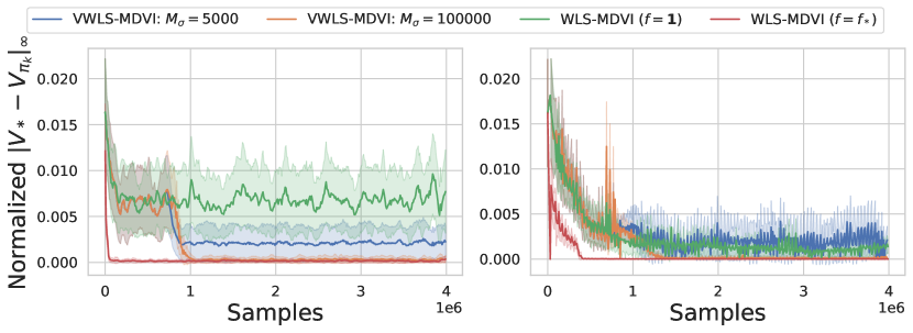
Figure 1: Comparison of the normalized gaps. VWLS-MDVI switches to the second run of WLS-MDVI around $10^{6}$ samples. Left: $M=\widetilde{M}=100$ and Right: $M=\widetilde{M}=1000$.

7 Experiments

This section reports the experimental sample efficiency of the proposed VWLS-MDVI and deep RL with DVW.

7.1 Linear MDP Experiments

To empirically validate the negative and positive claims made in Section 4.3 and demonstrate the sample efficiency of VWLS-MDVI, we compare VWLS-MDVI to WLS-MDVI with two different weighting functions: $f=\mathbf{1}$ and $f=f_{*}$, where $f_{*}\vcentcolon\nolinebreak\mkern-1.2mu=\min\mathopen{\lparen}\sigma(v_{*})+\sqrt{H}\mathbf{1},H\mathbf{1}\mathclose{\rparen}$ is the oracle weighting function from Theorem 4.4. The evaluation is conducted on randomly generated hard linear MDPs that are based on Theorem H.3 in Weisz et al. (2022). For simplicity, all algorithms use the last policy for evaluation. Specifically, for the $k\in[K]$ th iteration to update the parameter $\theta$, we report the normalized optimality gap $\mathopen{\lVert}v_{*}-v_{\pi_{k}}\mathclose{\rVert}_{\infty}/\mathopen{\lVert}v_{*}\mathclose{\rVert}_{\infty}$ in terms of the total number of samples used so far. We normalize the gap by $\mathopen{\lVert}v_{*}\mathclose{\rVert}_{\infty}$ as the maximum gap can vary depending on the MDPs.

Figure 1 compares algorithms under $M=\widetilde{M}=100$ (Left) and $M=\widetilde{M}=1000$ (Right). The results are averaged over $300$ random MDPs. For WLS-MDVI ($f=1$), increasing $M$ from 100 to 1000 results in a smaller optimality gap, which is expected due to the increase in the number of samples. On the other hand, WLS-MDVI ($f=f_{*}$) achieves a gap very close to $0$ even with $M=100$, demonstrating the effectiveness of variance-weighted regression in improving sample efficiency, as claimed in Section 4.3. Similarly, it is observed that the VWLS-MDVI ($M_{\sigma}=100000$) achieves a smaller gap with much fewer samples than that of WLS-MDVI. However, the gap of VWLS-MDVI ($M_{\sigma}=5000$) does not reach that of $f=f_{*}$. This suggests that the accuracy of the VarianceEstimation is important for guaranteeing good performance. Further experimental details are provided in LABEL:subsec:linear_mdp_details.

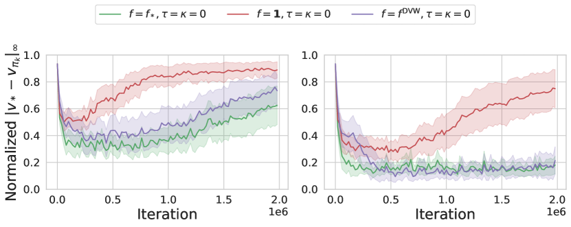
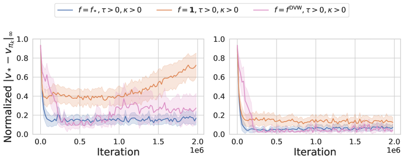
Figure 2: Comparison of the normalized gaps. Top Row: $\tau=\kappa=0$ and Bottom Row: $\tau>0,\kappa>0$. Left Column: $M=3$ and Right Column: $M=10$.

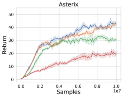
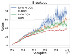
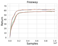
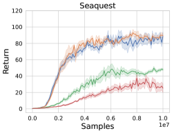
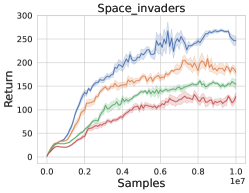
Figure 3: Comparison of returns on MinAtar benchmarks. We report the return of the greedy policy with respect to $q_{\theta}$ for each algorithm.

7.2 Deep RL Experiments

We perform two deep RL experiments to evaluate the effectiveness of DVW: one to compare DVW with the oracle weighting function of Theorem 4.4, and another to demonstrate the effectiveness of DVW to online deep RL. The details of the experiments are provided in Section 7.2.1.

7.2.1 Comparison of $f=f^{\text{DVW}}$ with $f\approx\sigma(v_{*})$

To investigate the effectiveness of DVW, we evaluate the behavior of M-DQN with weighted regression (8) under three weighting functions: the oracle weighting ($f=f_{*}$), the uniform weighting ($f=\mathbf{1}$), and the DVW weighting ($f=f^{\text{DVW}}$). Furthermore, for the purpose of ablation study, we compare the algorithms with and without regularization ($\tau>0,\kappa>0$ vs $\tau=0,\kappa=0$). To remove the challenge of exploration for didactic purposes, we use a dataset $\mathcal{B}$, which is constructed by pairs of $(x,a,r,x^{\prime})$ for the entire state-action space with $M$ next-state samples. In other words, $\mathcal{B}$ is a dataset of size $MXA$.

We evaluate them in randomly generated environments where we can compute oracle values. Specifically, we use a modified version of the gridworld environment described by Fu et al. (2019). For the $k$ th iteration to update the $q$-networks, we evaluate the normalized optimality gap averaged over $20$ environments and $3$ random seeds for each.

Figure 2 compares algorithms under $M=3$ (Left Column) and $M=10$ (Right Column). In both cases, DVW consistently achieves a smaller gap compared to $f=\mathbf{1}$, and moreover, the gap of DVW is comparable to that of the oracle weighting $f=f_{*}$. In addition, the gap is smaller when $\tau>0,\kappa>0$ compared to when $\tau=\kappa=0$. It can be inferred that DVW weighting and KL-entropy regularization contribute to improving sample efficiency, and that performance is significantly improved when both are present.

7.2.2 DVW for Online RL

We evaluate the effectiveness of DVW using a set of the challenging benchmarks for online RL. Similar to Section 7.2.1, we evaluate four algorithms that varied with and without DVW (DVW vs N/A), and with and without regularization (M-DQN vs DQN). We compare their performance on the MinAtar environment (Young & Tian, 2019), which possesses high-dimensional features and more challenging exploration than Section 7.2.1, while facilitating fast training. For a fair comparison, the algorithms use the same network architecture and same epsilon-greedy exploration strategy. Each algorithm is executed five times with different random seeds for each environment.

Figure 3 shows the average returns of the algorithms. We observe that DVW improves the performance of M-DQN and DQN in almost all the environments. Although our theory does not cover online RL, this experiment suggests that the extension of DVW to wider problem settings is effective.

8 Conclusion

In this study, we proposed both a theoretical algorithm, i.e., VWLS-MDVI, and a practical algorithm, i.e., DVW. VWLS-MDVI achieved the first-ever nearly minimax optimal sample complexity in infinite-horizon Linear MDPs by utilizing the combination of KL-entropy regularization and variance-weighted regression. We extended our theoretical observations and developed the DVW algorithm, which re-weights the least-squares loss of value-based RL algorithms using the estimated variance of the value function. Our experiments demonstrated that DVW effectively helps improve the performance of value-based deep RL algorithms.

Contents

• Appendix A lists notations for the theoretical analysis and their meaning;

• Appendix B proves the MDVI transformation stated in Section 3.1.2;

• Appendix C provides auxiliary lemmas necessary for proofs;

• Appendix E provides the formal theorem and the proofs of the total variance technique;

• Appendix F provides the proof of the existence of a small core set for a compact set (Theorem 3.3);

• Appendix G provides the proof of the weighted Kiefer Wolfowitz bound (Lemma 4.3);

• Appendix H provides the formal theorems and the proofs for sample complexity of WLS-MDVI (Theorem 4.4 and Theorem 5.1)

• LABEL:sec:evaluate_proof provides the formal theorem and the proof for sample complexity of VarianceEstimation (Theorem 5.2)

• LABEL:sec:proof_of_vwls_mdvi provides the formal theorem and the proof for sample complexity of VWLS-MDVI (Theorem 5.3);

• LABEL:appendix:missing_algorithms provides the pseudocode of algorithms missed in the main pages;

• LABEL:sec:experiment_details provides the details of experiments stated in Section 7.

Appendix A Notations for Theoretical Analysis

Table 2: Table of Notations for Theoretical Analysis

Notation	Meaning
$\mathcal{A}$, $\mathcal{X}$	action space of size $A$, state space
$\gamma$, $H$	discount factor in $[0,1)$ and effective horizon $H\vcentcolon\nolinebreak\mkern-1.2mu=1/(1-\gamma)$
$\phi$, $d$	feature map of a linear MDP and its dimension (3.2)
$r$	reward function bounded by $1$
$P$, $P_{\pi}$	transition kernel, $P_{\pi}\vcentcolon\nolinebreak\mkern-1.2mu=P\pi$
$\mathcal{F}_{v}$, $\mathcal{F}_{q}$	the sets of all bounded Borel-measurable functions over $\mathcal{X}$ and $\mathcal{X}\times\mathcal{A}$, respectively
$\pi_{k}^{\prime}$	a non-stationary policy that follows $\pi_{k},\pi_{k-1},\ldots$ sequentially (Section 3.1)
$P^{i}_{j}$, $P_{*}^{i}$	$P^{i}_{j}\vcentcolon\nolinebreak\mkern-1.2mu=P_{\pi_{i}}P_{\pi_{i-1}}\cdots P_{\pi_{j+1}}P_{\pi_{j}}$ and $P_{*}^{i}\vcentcolon\nolinebreak\mkern-1.2mu=(P_{\pi_{*}})^{i}$ (Section 3.1)
$T_{\pi}$, $T^{i}_{j}$	Bellman operator for a policy $\pi$, $T^{i}_{j}\vcentcolon\nolinebreak\mkern-1.2mu=T_{\pi_{i}}T_{\pi_{i-1}}\cdots T_{\pi_{j+1}}T_{\pi_{j}}$ (Section 3.1)
$v_{\pi^{\prime}_{k}}$	value function of $\pi^{\prime}_{k}$; $v_{\pi^{\prime}_{k}}=\pi_{k}T_{\pi_{k-1}}\cdots T_{\pi_{1}}q_{\pi_{0}}$.
$\varepsilon$, $\delta$	admissible suboptimality, admissible failure probability
$\varepsilon_{k}$	$\varepsilon_{k}:(x,a)\mapsto\gamma\widehat{P}_{k-1}(M)v_{k-1}(x,a)-\gamma Pv_{k-1}(x,a)$ in WLS-MDVI
$E_{k}$	$E_{k}:(x,a)\mapsto\sum_{j=1}^{k}\alpha^{k-j}\varepsilon_{j}(x,a)$
$f$	a bounded positive weighting function over $\mathcal{X}\times\mathcal{A}$
${\rho}_{f}$	a design over $\mathcal{X}\times\mathcal{A}$
${\mathcal{C}_{f}}$, $u_{\mathcal{C}}$	core set, $u_{\mathcal{C}}\vcentcolon\nolinebreak\mkern-1.2mu=4d\log\log(d+4)+28$ (Section 3.2)
${G_{f}}$	design matrix with respect to $f$, $\phi$, and ${\rho}_{f}$ (Theorem 4.1)
$u_{f},l_{f}$	$u_{f}\vcentcolon\nolinebreak\mkern-1.2mu=\max_{(x,a)\in\mathcal{X}\times\mathcal{A}}f(x,a)$, $l_{f}\vcentcolon\nolinebreak\mkern-1.2mu=\min_{(x,a)\in\mathcal{X}\times\mathcal{A}}f(x,a)$ (Appendix H)
$W(f_{1},f_{2})$	solution of a weighted least-squares estimation (Lemma 4.3)
$\widehat{P}_{k}$	$\widehat{P}_{k}(M)v_{k}:(x,a)\mapsto\frac{1}{M}\sum_{m=1}^{M}v_{k}(y_{k,m,x,a})$ (Section 3.1)
$\theta_{k}$, $\overline{\theta}_{k}$	parameter of $q_{k}$ in WLS-MDVI ($q_{k}=\phi^{\top}\theta_{k}$), $\overline{\theta}_{k}=\theta_{k}+\alpha\overline{\theta}_{k-1}=\sum^{k}_{j=0}\alpha^{k-j}\theta_{j}$
$\theta_{k}^{*}$, $\overline{\theta}_{k}^{*}$	parameter that satisfies $\phi^{\top}\theta^{*}_{k}=r+\gamma Pv_{k-1}$, ${\overline{\theta}}^{*}_{k}=\sum^{k}_{j=1}\alpha^{k-j}\theta^{*}_{j}$ (Appendix H)
$s_{k}$, $v_{k}$, $w_{k}$	$s_{k}\vcentcolon\nolinebreak\mkern-1.2mu=\phi^{\top}(x,a){\overline{\theta}}_{k}$, $v_{k}\vcentcolon\nolinebreak\mkern-1.2mu=w_{k}-\alpha w_{k-1}$, $w_{k}(x)\vcentcolon\nolinebreak\mkern-1.2mu=\max_{a\in\mathcal{A}}s_{k}(x,a)$ (WLS-MDVI)
$\alpha,\beta$	weights for MDVI updates $\alpha\vcentcolon\nolinebreak\mkern-1.2mu=\tau/(\tau+\kappa)$, $\beta\vcentcolon\nolinebreak\mkern-1.2mu=1/(\tau+\kappa)$ (Section 3.1)
$K,M$	the number of iterations and the number of samples from the generative model in WLS-MDVI
$\widehat{\mathrm{Var}}$	$\widehat{\mathrm{Var}}(x,a)=\frac{1}{2M}\sum_{m=1}^{M}\mathopen{\Bigl{\lparen}}v_{\sigma}(y_{m,x,a})-v_{\sigma}(z_{m,x,a})\mathclose{\Bigr{\rparen}}^{2}$ (Section 5.1)
$M_{\sigma}$	number of samples from the generative model in VarianceEstimation
$v_{\sigma}$	the input value function to VarianceEstimation
$\omega$	parameter for VarianceEstimation
$A_{k},A_{\infty},A_{\gamma,k}$	$\sum_{j=0}^{k-1}\alpha^{j}$, $\sum_{j=0}^{\infty}\alpha^{j}$, $\sum_{j=0}^{k-1}\alpha^{j}\gamma^{k-j}$
$\mathbf{F}_{k,m}$	$\sigma$-algebra in the filtration for WLS-MDVI (Appendix H)
$\mathbf{F}_{m}$	$\sigma$-algebra in the filtration for VarianceEstimation (LABEL:sec:evaluate_proof)
$\iota_{1}$, $\iota_{2,n}$	$\iota_{1}=\log(2c_{0}u_{\mathcal{C}}K\delta)$, $\iota_{2,n}=\log(2c_{0}^{2}u_{\mathcal{C}}K/(c_{0}-n)\delta)$ for $n\in\mathbb{N}$ (Appendix H)
$\xi_{2,n}$	$\xi_{2,n}=\iota_{2,n}+\log\log_{2}(16KH^{2})$ (Appendix H)
$\square$	an indefinite constant independent of $H$, $X$, $A$, $\varepsilon$, and $\delta$ (Appendix H)
E1	event of $f$ close to $\sigma(v_{*})$
E2	event of $v_{k}$ bound for all $k$
E3	event of small $E_{k}$ for all $k$ (not variance-aware)
E4	event of small $\varepsilon_{k}$ for all $k$ (not variance-aware)
E5	event of small $E_{k}$ for all $k$ (variance-aware)
E6	event of $v_{\sigma}$ close to $v_{*}$ (LABEL:sec:evaluate_proof)
E7	event of learned $\phi^{\top}\omega$ close to $\sigma(v_{*})$ (LABEL:sec:evaluate_proof)

Appendix B Equivalence of MDVI Update Rules (Kozuno et al., 2022)

We show the equivalence of MDVI’s updates (1) to those used in Tabular MDVI. The following transformation is identical to that of Kozuno et al. (2022) but is included here for completeness. We first recall MDVI’s updates (1):

$$q_{k+1}=r+\gamma\widehat{P}_{k}\pi_{k}\left\lparen q_{k}-\tau\log\frac{\pi_{k}}{\pi_{k-1}}-\kappa\log\pi_{k}\right\rparen\,,$$

$$\text{where }\pi_{k}\left\lparen\cdot\middle|x\right\rparen=\operatorname*{arg\,max}_{p\in\Delta(\mathcal{A})}\sum_{a\in\mathcal{A}}p(a)\left\lparen q_{k}(x,a)-\tau\log\frac{p(a)}{\pi_{k-1}\left\lparen a\middle|x\right\rparen}-\kappa\log p(a)\right\rparen\text{ for all }x\in\mathcal{X}\,,$$

The policy update can be rewritten in a closed-form solution as follows (e.g., Equation (5) of Kozuno et al. (2019)):

$$\pi_{k}(a|x)=\frac{\pi_{k-1}(a|x)^{\alpha}\exp\left\lparen\beta q_{k}(x,a)\right\rparen}{\sum_{b\in\mathcal{A}}\pi_{k-1}(b|x)^{\alpha}\exp\left\lparen\beta q_{k}(x,b)\right\rparen}\,,$$

where $\alpha\vcentcolon\nolinebreak\mkern-1.2mu=\tau/(\tau+\kappa)$, and $\beta\vcentcolon\nolinebreak\mkern-1.2mu=1/(\tau+\kappa)$. It can be further rewritten as, defining $s_{k}=q_{k}+\alpha s_{k-1}$,

$$\pi_{k}(a|x)=\frac{\exp\left\lparen\beta s_{k}(x,a)\right\rparen}{\sum_{b\in\mathcal{A}}\exp\left\lparen\beta s_{k}(x,b)\right\rparen}\,.$$

Plugging in this policy expression to $v_{k}$, we deduce that

$$v_{k}(x) =\frac{1}{\beta}\log\sum_{a\in\mathcal{A}}\exp\left\lparen\beta q_{k}(x,a)+\alpha\log\pi_{k-1}(a|x)\right\rparen$$

$$=\frac{1}{\beta}\log\sum_{a\in\mathcal{A}}\exp\left\lparen\beta s_{k}(x,a)\right\rparen-\frac{\alpha}{\beta}\log\sum_{a\in\mathcal{A}}\exp\left\lparen\beta s_{k-1}(x,a)\right\rparen\,.$$

Kozuno et al. (2019, Appendix B) show that when $\beta\to\infty$, $v_{k}(x)=w_{k}(x)-\alpha w_{k-1}(x)\,.$ Furthermore, the Boltzmann policy becomes a greedy policy. Accordingly, the update rules used in Tabular MDVI is a limit case of the original MDVI updates.

Appendix C Auxiliary Lemmas

In this appendix, we prove some auxiliary lemmas used in the proof. Some of the lemmas are identical to those of Kozuno et al. (2022) but are included here for completeness.

Lemma C.1.

For any events $A$ and $B$, $\mathbb{P}(A\cap B)\geq\mathbb{P}(B)-\mathbb{P}(A^{c}|B)$.

Proof.

$\mathbb{P}(A\cap B)=\mathbb{P}((A\cup B^{c})\cap B)\geq 1-\mathbb{P}(A^{c}\cap B)-\mathbb{P}(B^{c})=\mathbb{P}(B)-\mathbb{P}(A^{c}\cap B)\,.$ The claim holds by $\mathbb{P}(A^{c}\cap B)=\mathbb{P}(A^{c}|B)\mathbb{P}(B)\leq\mathbb{P}(A^{c}|B)$. ∎

Lemma C.2.

For any positive real values $a$ and $b$, $\sqrt{a+b}\leq\sqrt{a}+\sqrt{b}$.

Proof.

Indeed, $a+b\leq a+2\sqrt{ab}+b=(\sqrt{a}+\sqrt{b})^{2}$. ∎

Lemma C.3.

Let $a$, $b$, and $c$ are positive real values. If $|a^{2}-b^{2}|\leq c^{2}$, then $|a-b|\leq c$.

Proof.

Without loss of generality, assume that $a\geq b$. Then, $c^{2}\geq(a^{2}-b^{2})=(a+b)(a-b)\geq(a-b)^{2}$ and thus $|a-b|\leq c$. ∎

Lemma C.4.

For any real values $(a_{n})_{n=1}^{N}$, $(\sum_{n=1}^{N}a_{n})^{2}\leq N\sum_{n=1}^{N}a_{n}^{2}$.

Proof.

Indeed, from the Cauchy–Schwarz inequality,

$$\left\lparen\sum_{n=1}^{N}a_{n}\cdot 1\right\rparen^{2}\leq\left\lparen\sum_{n=1}^{N}1\right\rparen\left\lparen\sum_{n=1}^{N}a_{n}^{2}\right\rparen=N\sum_{n=1}^{N}a_{n}^{2}\,,$$

which is the desired result. ∎

Lemma C.5.

For any $k\in[K]$,

$$A_{\gamma,k}=\begin{cases}\gamma\dfrac{\alpha^{k}-\gamma^{k}}{\alpha-\gamma}&\text{if }\alpha\neq\gamma\\ k\gamma^{k}&\text{otherwise}\end{cases}\,.$$

Proof.

Indeed, if $\alpha\neq\gamma$

$$A_{\gamma,k}=\sum_{j=0}^{k-1}\alpha^{j}\gamma^{k-j}=\gamma^{k}\frac{(\alpha/\gamma)^{k}-1}{(\alpha/\gamma)-1}=\gamma\frac{\alpha^{k}-\gamma^{k}}{\alpha-\gamma}\,.$$

If $\alpha=\gamma$, $A_{\gamma,k}=k\gamma^{k}$ by definition. ∎

Lemma C.6.

For any real value $x\in(0,1]$, $1-x\leq\log(1/x)$.

Proof.

Since $\log(1/x)$ is convex and differentiable, $\log(1/x)\geq\log(1/y)-(x-y)/y$. Choosing $y=1$, we concludes the proof. ∎

Lemma C.7.

Suppose $\alpha,\gamma\in[0,1)$, $\varepsilon\in(0,1]$, $c\in[1,\infty)$, $m\in\mathbb{N}$, and $n\in[0,\infty)$. Let $K\vcentcolon\nolinebreak\mkern-1.2mu=\dfrac{m}{1-\alpha}\log\dfrac{cH}{\varepsilon}$. Then,

$$K^{n}\alpha^{K}\leq\left\lparen\frac{mn}{(1-\alpha)e}\right\rparen^{n}\left\lparen\dfrac{\varepsilon}{cH}\right\rparen^{m-1}\,.$$

Proof.

Using Lemma C.6 for $\alpha\in[0,1)$,

$$K=\frac{m}{1-\alpha}\log\dfrac{cH}{\varepsilon}\geq\log_{\alpha}\left\lparen\dfrac{\varepsilon}{cH}\right\rparen^{m}.$$

Therefore,

$$K^{n}\alpha^{K}\leq\left\lparen\frac{m}{1-\alpha}\log\dfrac{cH}{\varepsilon}\right\rparen^{n}\left\lparen\dfrac{\varepsilon}{cH}\right\rparen^{m}=\frac{m^{n}}{(1-\alpha)^{n}}\left\lparen\dfrac{\varepsilon}{cH}\right\rparen^{m}\left\lparen\log\dfrac{cH}{\varepsilon}\right\rparen^{n}\,.$$

Since $x\left\lparen\log\dfrac{1}{x}\right\rparen^{n}\leq\left\lparen\dfrac{n}{e}\right\rparen^{n}$ for any $x\in(0,1]$ as shown later,

$$K^{n}\alpha^{K}\leq\left\lparen\frac{mn}{(1-\alpha)e}\right\rparen^{n}\left\lparen\dfrac{\varepsilon}{cH}\right\rparen^{m-1}\,.$$

Now it remains to show $f(x)\vcentcolon\nolinebreak\mkern-1.2mu=x\left\lparen\log\dfrac{1}{x}\right\rparen^{n}\leq\left\lparen\dfrac{n}{e}\right\rparen^{n}$ for $x<1$. We have that

$$f^{\prime}(x)=(-\log x)^{n}-n(-\log x)^{n-1}\implies f^{\prime}(x)=0\text{ at }x=e^{-n}.$$

Therefore, $f$ takes its maximum $\left\lparen\dfrac{n}{e}\right\rparen^{n}$ at $e^{-n}$ when $x\in(0,1)$. ∎

The following lemma is a special case of a well-known inequality that for any increasing function $f$

$$\sum_{k=1}^{K}f(k)\leq\int_{1}^{K+1}f(x)dx\,.$$

Lemma C.8.

For any $K\in\mathbb{N}$ and $n\in[0,\infty)$, $\displaystyle\sum_{k=1}^{K}k^{n}\leq\frac{1}{n+1}(K+1)^{n+1}$.

Appendix D Tools from Probability Theory

We extensively use the following concentration inequality, which is derived based on a proof idea of Bernstein’s inequality (Bernstein, 1946; Boucheron et al., 2013) for a martingale (Lattimore & Szepesvari, 2020, Excercises 5.14 (f)). For a real-valued stochastic process $(X_{n})_{n=1}^{N}$ adapted to a filtration $(\mathcal{F}_{n})_{n=1}^{N}$, we let $\mathbb{E}_{n}[X_{n}]\vcentcolon\nolinebreak\mkern-1.2mu=\mathbb{E}\mathopen{[}X_{n}\mathord{|}\mathcal{F}_{n-1}\mathclose{]}$ for $n\geq 1$, and $\mathbb{E}_{1}[X_{1}]\vcentcolon\nolinebreak\mkern-1.2mu=\mathbb{E}\mathopen{[}X_{1}\mathclose{]}$.

Lemma D.1 (Azuma-Hoeffding Inequality).

Consider a real-valued stochastic process $(X_{n})_{n=1}^{N}$ adapted to a filtration $(\mathcal{F}_{n})_{n=1}^{N}$. Assume that $X_{n}\in[l_{n},u_{n}]$ and $\mathbb{E}_{n}[X_{n}]=0$ almost surely, for all $n$. Then,

$$\mathbb{P}\left\lparen\sum_{n=1}^{N}X_{n}\geq\sqrt{\sum_{n=1}^{N}\frac{(u_{n}-l_{n})^{2}}{2}\log\frac{1}{\delta}}\right\rparen\leq\delta$$

for any $\delta\in(0,1)$.

Lemma D.2 (Conditional Azuma-Hoeffding’s Inequality).

Consider a real-valued stochastic process $(X_{n})_{n=1}^{N}$ adapted to a filtration $(\mathcal{F}_{n})_{n=1}^{N}$. Assume that $\mathbb{E}_{n}[X_{n}]=0$ almost surely, for all $n$. Furthermore, let $\mathcal{E}$ be an event that implies $X_{n}\in[l_{n},u_{n}]$ with $\mathbb{P}(\mathcal{E})\geq 1-\delta^{\prime}$ for all $n$ and for some $\delta^{\prime}\in(0,1)$. Then,

$$\mathbb{P}\left\lparen\sum_{n=1}^{N}X_{n}\geq\sqrt{\sum_{n=1}^{N}\frac{(u_{n}-l_{n})^{2}}{2}\log\frac{1}{\delta(1-\delta^{\prime})}}\middle|\mathcal{E}\right\rparen\leq\delta$$

for any $\delta\in(0,1)$.

Proof.

Let $A$ denote the events of

$$\sum_{n=1}^{N}X_{n}\geq\sqrt{\sum_{n=1}^{N}\frac{(u_{n}-l_{n})^{2}}{2}\log\frac{1}{\delta(1-\delta^{\prime})}}\;.$$

Accordingly,

$$\mathbb{P}(A|\mathcal{E})=\frac{\mathbb{P}(A\cap\mathcal{E})}{\mathbb{P}(\mathcal{E})}\stackrel{{\scriptstyle\scriptscriptstyle(\mkern-1.5mua\mkern-1.5mu)}}{{\leq}}\frac{\delta(1-\delta^{\prime})}{\mathbb{P}(\mathcal{E})}\stackrel{{\scriptstyle\scriptscriptstyle(\mkern-1.5mub\mkern-1.5mu)}}{{\leq}}\delta\,,$$

where (a) follows from the Azuma-Hoeffding inequality (Lemma D.1), and (b) follows from $\mathbb{P}(\mathcal{E})\geq 1-\delta^{\prime}$. ∎

Lemma D.3 (Lemma 13 in Zhang et al. (2021)).

Consider a real-valued stochastic process $(X_{n})_{n=1}^{N}$ adapted to a filtration $(\mathcal{F}_{n})_{n=1}^{N}$. Suppose that $|X_{n}|\leq U$ and $\mathbb{E}_{n}[X_{n}]=0$ almost surely, for all $n$ and for some $U\in[0,\infty)$. Then, letting $V_{N}\vcentcolon\nolinebreak\mkern-1.2mu=\sum_{n=1}^{N}\mathbb{E}_{n}[X_{n}^{2}]$,

$$\mathbb{P}\left\lparen\left|\sum_{n=1}^{N}X_{n}\right|\geq 2\sqrt{2}\sqrt{V_{N}\log\left\lparen\frac{1}{\delta}\right\rparen}+2\sqrt{\epsilon\log\left\lparen\frac{1}{\delta}\right\rparen}+2U\log\left\lparen\frac{1}{\delta}\right\rparen\right\rparen\leq 2\left\lparen\log_{2}\left\lparen\frac{NU^{2}}{\epsilon}+1\right\rparen\right\rparen\delta\;,$$

for any $\epsilon,\delta>0$.

In our analysis, we use the following corollary of this inequality.

Lemma D.4 (Conditional Bernstein-type Inequality).

Consider a real-valued stochastic process $(X_{n})_{n=1}^{N}$ adapted to a filtration $(\mathcal{F}_{n})_{n=1}^{N}$. Suppose that $\mathbb{E}_{n}[X_{n}]=0$ almost surely, for all $n$. Furthermore, let $\mathcal{E}$ be an event that implies $|X_{n}|\leq U$ with $\mathbb{P}(\mathcal{E})\geq 1-\delta^{\prime}$ for all $n$, for some $\delta^{\prime}\in(0,1)$ and $U\in[0,\infty)$. Then, letting $V_{N}\vcentcolon\nolinebreak\mkern-1.2mu=\sum_{n=1}^{N}\mathbb{E}_{n}[X_{n}^{2}]$,

$$\mathbb{P}\left\lparen\left|\sum_{n=1}^{N}X_{n}\right|\geq 2\sqrt{2}\sqrt{(1+V_{N})\log\left\lparen\frac{2\log_{2}\left\lparen NU^{2}\right\rparen}{\delta(1-\delta^{\prime})}\right\rparen}+2U\log\left\lparen\frac{2\log_{2}(NU^{2})}{\delta(1-\delta^{\prime})}\right\rparen\middle|\mathcal{E}\right\rparen\leq\delta\;,$$

for any $\delta>0$.

Proof.

Let $A$ and $B$ denote the events of

$$\left|\sum_{n=1}^{N}X_{n}\right|\geq 2\sqrt{2}\sqrt{(1+V_{N})\log\left\lparen\frac{2\log_{2}(NU^{2})}{\delta(1-\delta^{\prime})}\right\rparen}+2U\log\left\lparen\frac{2\log_{2}(NU^{2})}{\delta(1-\delta^{\prime})}\right\rparen\;$$

and $|X_{n}|\leq U$ for all $n$, respectively. Since $\mathcal{E}\subset B$, it follows that $A\cap\mathcal{E}\subset A\cap B$, and $\mathbb{P}(A\cap\mathcal{E})\leq\mathbb{P}(A\cap B)$. Accordingly,

$$\mathbb{P}(A|\mathcal{E})=\frac{\mathbb{P}(A\cap\mathcal{E})}{\mathbb{P}(\mathcal{E})}\leq\frac{\mathbb{P}(A\cap B)}{\mathbb{P}(\mathcal{E})}\stackrel{{\scriptstyle\scriptscriptstyle(\mkern-1.5mua\mkern-1.5mu)}}{{\leq}}\frac{\delta(1-\delta^{\prime})}{\mathbb{P}(\mathcal{E})}\stackrel{{\scriptstyle\scriptscriptstyle(\mkern-1.5mub\mkern-1.5mu)}}{{\leq}}\delta\,,$$

where (a) follows from Lemma D.3 with $1+\sqrt{V_{N}}\geq\sqrt{1+V_{N}}$ due to Lemma C.2 and $\epsilon=2$. Then, (b) follows from $\mathbb{P}(\mathcal{E})\geq 1-\delta^{\prime}$. ∎

Lemma D.5 (Popoviciu’s Inequality for Variances).

The variance of any random variable bounded by $x$ is bounded by $x^{2}$.

Appendix E Total Variance Technique (Kozuno et al., 2022)

This section introduces the total variance technique for non-stationary policy. The proof is identical to that of Kozuno et al. (2022) but is included here for completeness.

The following lemma is due to Azar et al. (2013).

Lemma E.1.

Suppose two real-valued random variables $X,Y$ whose variances, $\mathbb{V}X$ and $\mathbb{V}Y$, exist and are finite. Then, $\sqrt{\mathbb{V}X}\leq\sqrt{\mathbb{V}\left[X-Y\right]}+\sqrt{\mathbb{V}Y}$.

For completeness, we prove Lemma E.1.

Proof.

Indeed, from Cauchy-Schwartz inequality,

$$\mathbb{V}X =\mathbb{V}\mathopen{[}X-Y+Y\mathclose{]}$$

$$=\mathbb{V}\mathopen{[}X-Y\mathclose{]}+\mathbb{V}Y+2\mathbb{E}\left[(X-Y-\mathbb{E}\mathopen{[}X-Y\mathclose{]})(Y-\mathbb{E}Y)\right]$$

$$\leq\mathbb{V}\mathopen{[}X-Y\mathclose{]}+\mathbb{V}Y+2\sqrt{\mathbb{V}\mathopen{[}X-Y\mathclose{]}\mathbb{V}Y}=\left\lparen\sqrt{\mathbb{V}\left[X-Y\right]}+\sqrt{\mathbb{V}Y}\right\rparen^{2}\,.$$

This is the desired result. ∎

The following lemma is an extension of Lemma 7 by Azar et al. (2013) and its refined version by Agarwal et al. (2020).

Lemma E.2.

Suppose a sequence of deterministic policies $(\pi_{k})_{k=0}^{K}$ and let

$$q_{\pi^{\prime}_{k}}\vcentcolon\nolinebreak\mkern-1.2mu=\begin{cases}r+\gamma Pv_{\pi^{\prime}_{k-1}}&\text{for }k\in[K]\\ q_{\pi_{0}}&\text{for }k=0\end{cases}\,.$$

Furthermore, let $\sigma_{k}^{2}$ and $\Sigma_{k}^{2}$ be non-negative functions over $\mathcal{X}\times\mathcal{A}$ defined by

$$\sigma_{k}^{2}(x,a)\vcentcolon\nolinebreak\mkern-1.2mu=\begin{cases}P\mathopen{\lparen}v_{\pi^{\prime}_{k-1}}\mathclose{\rparen}^{2}(x,a)-\mathopen{\lparen}Pv_{\pi^{\prime}_{k-1}}\mathclose{\rparen}^{2}(x,a)&\text{for }k\in[K]\\ P\mathopen{\lparen}v_{\pi_{0}}\mathclose{\rparen}^{2}(x,a)-\mathopen{\lparen}Pv_{\pi_{0}}\mathclose{\rparen}^{2}(x,a)&\text{for }k=0\end{cases}$$

and

$$\Sigma_{k}^{2}(x,a)\vcentcolon\nolinebreak\mkern-1.2mu=\mathbb{E}_{k}\left[\left\lparen\sum_{t=0}^{\infty}\gamma^{t}r(X_{t},A_{t})-q_{\pi^{\prime}_{k}}(X_{0},A_{0})\right\rparen^{2}\middle|X_{0}=x,A_{0}=a\right]$$ (12)

for $k\in\{0\}\cup[K]$, where $\mathbb{E}_{k}$ is the expectation over $(X_{t},A_{t})_{t=0}^{\infty}$ wherein $A_{t}\sim\pi_{k-t}(\cdot|X_{t})$ until $t=k$, and $A_{t}\sim\pi_{0}(\cdot|X_{t})$ thereafter. Then,

$$\sum_{j=0}^{k-1}\gamma^{j+1}P_{k-j}^{k-1}\sigma_{k-j}\leq\sqrt{2H^{3}}\mathbf{1}$$

for any $k\in[K]$.

For its proof, we need the following lemma.

Lemma E.3.

Suppose a sequence of deterministic policies $(\pi_{k})_{k=0}^{K}$ and notations in Lemma E.2. Then, for any $k\in[K]$, we have that

$$\Sigma_{k}^{2}=\gamma^{2}\sigma_{k}^{2}+\gamma^{2}P_{\pi_{k-1}}\Sigma_{k-1}^{2}\,.$$

Proof.

Let $R_{s}^{u}\vcentcolon\nolinebreak\mkern-1.2mu=\sum_{t=s}^{u}\gamma^{t-s}r(X_{t},A_{t})$ and $\mathbb{E}_{k}\left[\cdot\middle|x,a\right]\vcentcolon\nolinebreak\mkern-1.2mu=\mathbb{E}_{k}\left[\cdot\middle|X_{0}=x,A_{0}=a\right]$. We have that

$$\Sigma_{k}^{2}(x,a)=\mathbb{E}_{k}\left[\left\lparen R_{0}^{\infty}-q_{\pi^{\prime}_{k}}(X_{0},A_{0})\right\rparen^{2}\middle|x,a\right]\vcentcolon\nolinebreak\mkern-1.2mu=\mathbb{E}_{k}\left[\left\lparen I_{1}+\gamma I_{2}\right\rparen^{2}\middle|x,a\right]\,,$$

where $I_{1}\vcentcolon\nolinebreak\mkern-1.2mu=r(X_{0},A_{0})+\gamma q_{\pi^{\prime}_{k-1}}(X_{1},A_{1})-q_{\pi^{\prime}_{k}}(X_{0},A_{0})$, and $I_{2}\vcentcolon\nolinebreak\mkern-1.2mu=R_{1}^{\infty}-q_{\pi^{\prime}_{k-1}}(X_{1},A_{1})$. With these notations, we see that

$$\Sigma_{k}^{2}(x,a) =\mathbb{E}_{k}\mathopen{\bigl{[}}I_{1}^{2}+\gamma^{2}I_{2}^{2}+2\gamma I_{1}I_{2}\mathord{\bigm{|}}x,a\mathclose{\bigr{]}}$$

$$=\mathbb{E}_{k}\mathopen{\bigl{[}}I_{1}^{2}+\gamma^{2}I_{2}^{2}+2\gamma I_{1}\mathbb{E}_{k-1}\left[I_{2}\middle|X_{1},A_{1}\right]\mathord{\bigm{|}}x,a\mathclose{\bigr{]}}$$

$$=\mathbb{E}_{k}\mathopen{\bigl{[}}I_{1}^{2}\mathord{\bigm{|}}x,a\mathclose{\bigr{]}}+\gamma^{2}\mathbb{E}_{k}\mathopen{\bigl{[}}I_{2}^{2}\mathord{\bigm{|}}x,a\mathclose{\bigr{]}}$$

$$=\mathbb{E}_{k}\mathopen{\bigl{[}}I_{1}^{2}\mathord{\bigm{|}}x,a\mathclose{\bigr{]}}+\gamma^{2}P^{\pi_{k-1}}\Sigma_{k-1}^{2}(x,a)\,,$$

where the second line follows from the law of total expectation, and the third line follows since $\mathbb{E}_{k-1}\left[I_{2}\middle|X_{1},A_{1}\right]=0$ due to the Markov property. The first term in the last line is $\gamma^{2}\sigma_{k}^{2}(x,a)$ because

$$\mathbb{E}_{k}\mathopen{\bigl{[}}I_{1}^{2}\mathord{\bigm{|}}x,a\mathclose{\bigr{]}} \stackrel{{\scriptstyle\scriptscriptstyle(\mkern-1.5mua\mkern-1.5mu)}}{{=}}\gamma^{2}\mathbb{E}_{k}\mathopen{\Biggl{[}}\mathopen{\Bigl{\lparen}}\underbrace{q_{\pi_{k-1}^{\prime}}(X_{1},A_{1})}_{v_{\pi_{k-1}^{\prime}}(X_{1})\text{ from (b)}}-(Pv_{\pi_{k-1}^{\prime}})(X_{0},A_{0})\mathclose{\Bigr{\rparen}}^{2}\mathord{\Biggm{|}}x,a\mathclose{\Biggr{]}}$$

$$=\gamma^{2}\left\lparen P\left\lparen v_{\pi_{k-1}^{\prime}}\right\rparen^{2}\right\rparen(x,a)+\gamma^{2}(Pv_{\pi_{k-1}^{\prime}})^{2}(x,a)-2(Pv_{\pi_{k-1}^{\prime}})^{2}(x,a)$$

$$=\gamma^{2}\left\lparen P\left\lparen v_{\pi_{k-1}^{\prime}}\right\rparen^{2}\right\rparen(x,a)-\gamma^{2}(Pv_{\pi_{k-1}^{\prime}})^{2}(x,a)\,,$$

where (a) follows from the definition that $q_{\pi_{k}^{\prime}}=r+\gamma Pv_{\pi^{\prime}_{k-1}}$, and (b) follows since the policies are deterministic. From this argument, it is clear that $\Sigma_{k}^{2}=\gamma^{2}\sigma_{k}^{2}+\gamma^{2}P_{\pi_{k-1}}\Sigma_{k-1}^{2}\,,$ which is the desired result. ∎

Now, we are ready to prove Lemma E.2.

Proof of Lemma E.2.

Let $H_{k}\vcentcolon\nolinebreak\mkern-1.2mu=\sum_{j=0}^{k-1}\gamma^{j}$. Using Jensen’s inequality twice,

$$\sum_{j=0}^{k-1}\gamma^{j+1}P_{k-j}^{k-1}\sigma_{k-j} \leq\sum_{j=0}^{k-1}{\gamma^{j+1}\sqrt{P_{k-j}^{k-1}\sigma_{k-j}^{2}}}$$

$$\leq\gamma H_{k}\sum_{j=0}^{k-1}{\frac{\gamma^{j+1}}{H_{k}}\sqrt{P_{k-j}^{k-1}\sigma_{k-j}^{2}}}$$

$$\leq\sqrt{H_{k}\sum_{j=0}^{k-1}{\gamma^{j+2}P_{k-j}^{k-1}\sigma_{k-j}^{2}}}\leq\sqrt{H\sum_{j=0}^{k-1}{\gamma^{j+2}P_{k-j}^{k-1}\sigma_{k-j}^{2}}}\,.$$

From Lemma E.3, we have that

$$\sum_{j=0}^{k-1}{\gamma^{j+2}P_{k-j}^{k-1}\sigma_{k-j}^{2}} =\sum_{j=0}^{k-1}{\gamma^{j}P_{k-j}^{k-1}\left\lparen\Sigma_{k-j}^{2}-\gamma^{2}P^{\pi_{k-1-j}}\Sigma_{k-1-j}^{2}\right\rparen}$$

$$=\sum_{j=0}^{k-1}{\gamma^{j}P_{k-j}^{k-1}\left\lparen\Sigma_{k-j}^{2}-\gamma P^{\pi_{k-1-j}}\Sigma_{k-1-j}^{2}+\gamma(1-\gamma)P^{\pi_{k-1-j}}\Sigma_{k-1-j}^{2}\right\rparen}$$

$$=\sum_{j=0}^{k-1}\gamma^{j}P_{k-j}^{k-1}\Sigma_{k-j}^{2}-\sum_{j=1}^{k}\gamma^{j}P_{k-j}^{k-1}\Sigma_{k-j}^{2}+\gamma(1-\gamma)\sum_{j=0}^{k-1}\gamma^{j}P_{k-1-j}^{k-1}\Sigma_{k-1-j}^{2}\,.$$

The final line is equal to $\Sigma_{k}^{2}-\gamma^{k}P_{0}^{k-1}\Sigma_{0}^{2}+\gamma(1-\gamma)\sum_{j=0}^{k-1}\gamma^{j}P_{k-1-j}^{k-1}\Sigma_{k-1-j}^{2}$. Finally, from the monotonicity of stochastic matrices and that $\mathbf{0}\leq\Sigma_{j}^{2}\leq H^{2}\mathbf{1}$ for any $j$,

$$\sum_{j=0}^{k-1}\gamma^{j+1}P_{k-j}^{k-1}\sigma_{k-j}\leq\sqrt{2H^{3}}\mathbf{1}\,.$$

This concludes the proof. ∎

Appendix F Proof of Theorem 3.3

As a reminder, let $\Phi\vcentcolon\nolinebreak\mkern-1.2mu=\{\phi(x,a):(x,a)\in\mathcal{X}\times\mathcal{A}\}\subset\mathbb{R}^{d}$. For $G\in\mathbb{R}^{d\times d}$ and $\phi\in\mathbb{R}^{d}$, we use the notation $\|\phi\|_{G}^{2}:=\phi^{\top}G\phi$. Additionally, we use the operator norm of a matrix $G$ and denote it as $\|G\|=\sup_{\phi^{\top}\phi=1}\sqrt{(G\phi)^{\top}G\phi}$.

We first introduce an algorithm for computing the G-optimal design for finite $\mathcal{X}$, called the Frank-Wolfe algorithm from Todd (2016). The pseudocode is provided in LABEL:algo:frank_wolfe. The following theorem shows that LABEL:algo:frank_wolfe outputs a near-optimal design with a small core set.

Theorem F.1 (Proposition 3.17, Todd (2016)).

Let $u_{\mathcal{C}}\vcentcolon\nolinebreak\mkern-1.2mu=4d\log\log(d+4)+28$. For $\Phi$ satisfying 3.2 and if $\Phi$ is finite, LABEL:algo:frank_wolfe with $f:\mathcal{X}\times\mathcal{A}\to(0,\infty)$ and $\varepsilon^{\mathrm{FW}}=d$ outputs a design $\rho$ such that $g(\rho)\leq 2d$ and the core set $C$ with size at most $u_{\mathcal{C}}$.

We extend the theorem to a compact $\Phi$ by passing to the limit. The proof of Theorem 3.3 is a modification of Exercise 21.3 in Lattimore & Szepesvari (2020).

Proof of Theorem 3.3.

Suppose that $\Phi$ satisfies 3.2 such that $\Phi$ is a compact subset of $\mathbb{R}^{d}$ and spans $\mathbb{R}^{d}$. Let $\left(\Phi_{n}\right)_{n}$ be a sequence of finite subsets with $\Phi_{n}\subset\Phi_{n+1}$. We suppose that $\Phi_{n}$ spans $\mathbb{R}^{d}$ and $\lim_{n\rightarrow\infty}D\left(\Phi,\Phi_{n}\right)=0$ where $D$ is the Hausdorff metric. Then let $\rho_{n}$ be a $G$-optimal design for $\Phi_{n}$ with support of size at most $u_{\mathcal{C}}$ and $G_{n}\vcentcolon\nolinebreak\mkern-1.2mu=\sum_{(x,a)\in\mathcal{X}\times\mathcal{A}}\rho_{n}(x,a)\phi(x,a)\phi(x,a)^{\top}$. Such the design is ensured to exist by Theorem F.1. Given any $\phi\in\Phi$, we have

$$\|\phi\|_{G_{n}^{-1}}\leq\min_{b\in\Phi_{n}}\left(\|\phi-b\|_{G_{n}^{-1}}+\|b\|_{G_{n}^{-1}}\right)\leq\sqrt{2d}+\min_{b\in\Phi_{n}}\|\phi-b\|_{G_{n}^{-1}}\;,$$ (13)

where the first inequality is due to the triangle inequality and the second inequality is due to Theorem F.1. Let $W\in\mathbb{R}^{d\times d}$ be an invertible matrix and $w_{i}\in\mathbb{R}^{d}$ be its $i\in[d]$ th column. We suppose that $w_{i}\in\Phi$ for any $i\in[d]$. Such $W$ can be constructed due to the assumption that $\Phi$ spans $\mathbb{R}^{d}$. Then, the operator norm of $G^{-1/2}_{n}$ is bounded by

$$\left\|G_{n}^{-1/2}\right\|=\left\|W^{-1}WG_{n}^{-1/2}\right\|\leq\left\|W^{-1}\right\|\left\|G_{n}^{-1/2}W\right\|=\left\|W^{-1}\right\|\sup_{\phi^{\top}\phi=1}\|W\phi\|_{G_{n}^{-1}}\;,$$ (14)

where the last equality is due to $\left\|G_{n}^{-1/2}W\right\|=\sup_{\phi^{\top}\phi=1}\sqrt{(G_{n}^{-1/2}W\phi)^{\top}G_{n}^{-1/2}W\phi}=\sup_{\phi^{\top}\phi=1}\|W\phi\|_{G_{n}^{-1}}$. Let $\phi_{i}$ be the $i$ th element of $\phi\in\mathbb{R}^{d}$. Equation 14 is further bounded by

$$\sup_{\phi^{\top}\phi=1}\|W\phi\|_{G_{n}^{-1}}\leq\sup_{\phi^{\top}\phi=1}\sum_{i=1}^{d}\left|\phi_{i}\right|\underbrace{\left\|w_{i}\right\|_{G_{n}^{-1}}}_{\leq\sqrt{2d}}\leq 2d\;.$$

Therefore, we have $\left\|G_{n}^{-1/2}\right\|\leq 2d\left\|W^{-1}\right\|$. Taking the limit $n\to\infty$ shows that

$$\limsup_{n\rightarrow\infty}\|\phi\|_{G_{n}^{-1}} \stackrel{{\scriptstyle\scriptscriptstyle(\mkern-1.5mua\mkern-1.5mu)}}{{\leq}}\sqrt{2d}+\limsup_{n\rightarrow\infty}\min_{b\in\Phi}\|\phi-b\|_{G_{n}^{-1}}$$

$$\stackrel{{\scriptstyle\scriptscriptstyle(\mkern-1.5mub\mkern-1.5mu)}}{{\leq}}\sqrt{2d}+2d\left\|W^{-1}\right\|\limsup_{n\rightarrow\infty}\min_{b\in\Phi}\sqrt{(\phi-b)^{\top}(\phi-b)}=\sqrt{2d}\;,$$

where (a) is due to (13) and (b) uses $\left\|G_{n}^{-1/2}\right\|\leq 2d\left\|W^{-1}\right\|$.

Since $\|\cdot\|_{G_{n}^{-1}}:\Phi\rightarrow\mathbb{R}$ is continuous and $\Phi$ is compact, it follows that

$$\limsup_{n\rightarrow\infty}\sup_{\phi\in\Phi}\|\phi\|_{G_{n}^{-1}}^{2}\leq 2d\;.$$ (15)

Notice that $\rho_{n}$ may be represented as a tuple of vector/probability pairs with at most $u_{\mathcal{C}}$ entries and where the vectors lie in $\Phi$. Since the set of all such tuples with the obvious topology forms a compact set, it follows that $\left(\rho_{n}\right)$ has a cluster point $\rho^{*}$, which represents a distribution on $\Phi$ with support at most $u_{\mathcal{C}}$. Then, Equation 15 shows that $g\left(\rho^{*}\right)\leq 2d$. This concludes the proof. ∎

Appendix G Proof of Weighted KW Bound (Lemma 4.3)

Proof.

$\left|\phi^{\top}(x,a)W(f,z)\right|$ can be rewritten as

$$\left|\phi^{\top}(x,a)W(f,z)\right| =\left|\phi^{\top}(x,a)G_{f}^{-1}\sum_{(y,b)\in\mathcal{C}_{f}}\rho_{f}(y,b)\frac{\phi(y,b)}{f(y,b)}\frac{z(y,b)}{f(y,b)}\right|$$ (16)

$$\stackrel{{\scriptstyle\scriptscriptstyle(\mkern-1.5mua\mkern-1.5mu)}}{{\leq}}\left|\sum_{(y,b)\in\mathcal{C}_{f}}\rho_{f}(y,b)\phi^{\top}(x,a)G_{f}^{-1}\frac{\phi(y,b)}{f(y,b)}\right|\max_{({y^{\prime},b^{\prime}})\in\mathcal{C}_{f}}\left|\frac{z(y^{\prime},b^{\prime})}{f(y^{\prime},b^{\prime})}\right|$$

$$\stackrel{{\scriptstyle\scriptscriptstyle(\mkern-1.5mub\mkern-1.5mu)}}{{\leq}}\sum_{(y,b)\in\mathcal{C}_{f}}\left|\rho_{f}(y,b)\phi^{\top}(x,a)G_{f}^{-1}\frac{\phi(y,b)}{f(y,b)}\right|\max_{({y^{\prime},b^{\prime}})\in\mathcal{C}_{f}}\left|\frac{z(y^{\prime},b^{\prime})}{f(y^{\prime},b^{\prime})}\right|\;,$$

where (a) is due to Hölder’s inequality and (b) is due to the triangle inequality.

Next, for any $(x,a)\in\mathcal{X}\times\mathcal{A}$, we have

$$\left(\sum_{(y,b)\in\mathcal{C}_{f}}\left|\rho_{f}(y,b)\phi(x,a)^{\top}G_{f}^{-1}\frac{\phi(y,b)}{f(y,b)}\right|\right)^{2} \stackrel{{\scriptstyle\scriptscriptstyle(\mkern-1.5mua\mkern-1.5mu)}}{{\leq}}\sum_{(y,b)\in\mathcal{C}_{f}}\rho_{f}(y,b)\left|\phi(x,a)^{\top}G_{f}^{-1}\frac{\phi(y,b)}{f(y,b)}\right|^{2}$$ (17)

$$\stackrel{{\scriptstyle\scriptscriptstyle(\mkern-1.5mub\mkern-1.5mu)}}{{=}}f^{2}(x,a)\underbrace{\frac{\phi(x,a)^{\top}}{f(x,a)}G_{f}^{-1}\frac{\phi(x,a)}{f(x,a)}}_{\leq 2d\text{ from \lx@cref{creftype~refnum}{theorem:weighted KW}}}$$

where (a) is due to Jensen’s inequality, (b) is due to the definition of $G_{f}$. The claim holds by taking the square root for both sides of the inequality (17) and applying the result to the inequality (16). ∎

Appendix H Formal Theorems and Proofs of Theorem 4.4 and Theorem 5.1

This section provides the concrete proofs of Theorem 4.4 and Theorem 5.1. Instead of the informal theorems of Theorem 4.4 and Theorem 5.1, we are going to prove the formal theorems below, Theorem H.1 and Theorem H.2, respectively.

Theorem H.1 (Sample complexity of WLS-MDVI with $f\approx\sigma(v_{*})$).

Let $c_{0}$ be a positive constant such that $8\geq c_{0}\geq 6$ and $\widetilde{\sigma}\in\mathcal{F}_{q}$ be a random variable. Assume that $\varepsilon\in(0,1/H]$ and an event

$$\sigma(v_{*})\leq\widetilde{\sigma}\leq\sigma(v_{*})+2\sqrt{H}\mathbf{1}\;$$

occurs with probability at least $1-4\delta/c_{0}$. Define

$$f^{\text{wls}}\vcentcolon\nolinebreak\mkern-1.2mu=\max\left\lparen\min(\widetilde{\sigma},H\mathbf{1}),\sqrt{H}\mathbf{1}\right\rparen\,,$$

$$K^{\text{wls}}\vcentcolon\nolinebreak\mkern-1.2mu=\left\lceil\frac{3}{1-\alpha}\log{{c_{1}H}}+1\right\rceil\,,$$

and $$M^{\text{wls}}\vcentcolon\nolinebreak\mkern-1.2mu=\left\lceil{\frac{c_{2}dH^{2}}{\varepsilon^{2}}\log\left\lparen\frac{2c_{0}^{2}u_{\mathcal{C}}K^{\text{wls}}}{(c_{0}-5)\delta}\log_{2}\frac{16K^{\text{wls}}H^{2}}{(c_{0}-5)\delta}\right\rparen}\right\rceil\,$$

where $c_{1},c_{2}\geq 1$ are positive constants and $u_{\mathcal{C}}=4d\log\log(d+4)+28$. Then, there exist $c_{1},c_{2}\geq 1$ independent of $d$, $H$, $X$, $A$, $\varepsilon$, and $\delta$ such that WLS-MDVI is run with the settings $\alpha=\gamma$, $f=f^{\text{wls}}$, $K=K^{\text{wls}}$, $M=M^{\text{wls}}$ it outputs a sequence of policies $(\pi_{k})_{k=0}^{K}$ such that $\mathopen{\lVert}v_{*}-v_{\pi^{\prime}_{K}}\mathclose{\rVert}_{\infty}\leq\varepsilon$ with probability at least $1-\delta$, using $\widetilde{\mathcal{O}}\left\lparen u_{\mathcal{C}}KM\right\rparen=\widetilde{\mathcal{O}}\left\lparen d^{2}H^{3}/\varepsilon^{2}\right\rparen$ samples from the generative model.

Theorem H.2 (Sapmle complexity of WLS-MDVI with $f=\mathbf{1}$).

Assume that $\varepsilon\in(0,1/H]$. Let $c_{0}$ be a positive constant such that $8\geq c_{0}\geq 6$. Define

$$K^{\text{ls}}\vcentcolon\nolinebreak\mkern-1.2mu=\left\lceil\frac{3}{1-\alpha}\log{c_{3}H}+1\right\rceil\,$$

and $$M^{\text{ls}}\vcentcolon\nolinebreak\mkern-1.2mu=\left\lceil\frac{c_{4}dH^{2}}{\varepsilon}\log{\frac{2c_{0}^{2}u_{\mathcal{C}}K^{\text{ls}}}{(c_{0}-5)\delta}}\right\rceil\,$$

where $c_{3},c_{4}\geq 1$ are positive constants and $u_{\mathcal{C}}=4d\log\log(d+4)+28$. Then, there exist $c_{3},c_{4}\geq 1$ independent of $d$, $H$, $X$, $A$, $\varepsilon$ and $\delta$ such that when WLS-MDVI is run with the settings $\alpha=\gamma$, $f=\mathbf{1}$, $K=K^{\text{ls}}$, and $M=M^{\text{ls}}$, it outputs $v_{K}$ such that $\mathopen{\lVert}v_{*}-v_{K}\mathclose{\rVert}_{\infty}\leq\frac{1}{2}\sqrt{H}$ with probability at least $1-3\delta/c_{0}$, using $\widetilde{\mathcal{O}}\left\lparen u_{\mathcal{C}}KM\right\rparen=\widetilde{\mathcal{O}}\left\lparen d^{2}H^{3}/\varepsilon\right\rparen$ samples from the generative model.

The proof sketch is provided in Section H.2.

H.1 Notation and Frequently Used Facts for Proofs

Before moving on to the proofs, we introduce some notations and frequently used facts for theoretical analysis.

Notation for proofs.

$\square$ denotes an indefinite constant that changes throughout the proof and is independent of $d$, $H$, $X$, $A$, $\varepsilon$, and $\delta$.

For a sequence of policies $(\pi_{k})_{k\in\mathbb{Z}}$, we let $T_{j}^{i}\vcentcolon\nolinebreak\mkern-1.2mu=T_{\pi_{i}}T_{\pi_{i-1}}\cdots T_{\pi_{j+1}}T_{\pi_{j}}$ for $i\geq j$, and $T_{j}^{i}\vcentcolon\nolinebreak\mkern-1.2mu=I$ otherwise.

For $k\in\{1,\ldots,N\}$, we write $\theta^{*}_{k}\in\mathbb{R}^{d}$ as the underlying unknown parameter vector satisfying $\phi^{\top}\theta^{*}_{k}=r+\gamma Pv_{k-1}$. $\theta^{*}_{k}$ is ensured to exist by the property of linear MDPs. We also write $\overline{\theta}^{*}_{k}$ as its past moving average, i.e., ${\overline{\theta}}^{*}_{k}=\sum^{k}_{j=1}\alpha^{k-j}\theta^{*}_{j}$.

For Theorem H.2, $\mathbf{F}_{k,m}$ denotes the $\sigma$-algebra generated by random variables $\{y_{j,n,x,a}|(j,n,x,a)\in[k-2]\times[M]\times\mathcal{X}\times\mathcal{A}\}\cup\{y_{j,n,x,a}|(j,n,x,a)\in\{k-1\}\times[m-1]\times\mathcal{X}\times\mathcal{A}\}$. With an abuse of notation, for Theorem H.1, $\mathbf{F}_{k,m}$ denotes the $\sigma$-algebra generated by random variables $\{\widetilde{\sigma}\}\cup\{y_{j,n,x,a}|(j,n,x,a)\in[k-2]\times[M]\times\mathcal{X}\times\mathcal{A}\}\cup\{y_{j,n,x,a}|(j,n,x,a)\in\{k-1\}\times[m-1]\times\mathcal{X}\times\mathcal{A}\}$. Whether $\mathbf{F}_{k,m}$ is for Theorem H.2 or Theorem H.1 shall be clear from the context.

For the bounded positive function $f$ used in WLS-MDVI, we introduce the shorthand $u_{f}\vcentcolon\nolinebreak\mkern-1.2mu=\max_{(x,a)\in\mathcal{X}\times\mathcal{A}}f(x,a)$ and $l_{f}\vcentcolon\nolinebreak\mkern-1.2mu=\min_{(x,a)\in\mathcal{X}\times\mathcal{A}}f(x,a)$.

Finally, throughout the proof, for $8\geq c_{0}>n>0$, we write $\iota_{1}\vcentcolon\nolinebreak\mkern-1.2mu=\log(2c_{0}u_{\mathcal{C}}K/\delta)$, $\iota_{2,n}\vcentcolon\nolinebreak\mkern-1.2mu=\iota_{1}+\log(c_{0}/(c_{0}-n))=\log(2c_{0}^{2}u_{\mathcal{C}}K/(c_{0}-n)\delta)$, and $\xi_{2,n}\vcentcolon\nolinebreak\mkern-1.2mu=\iota_{2,n}+\log\log_{2}(16KH^{2})$. Note that for any $8\geq c_{0}>n>0$,

$$\xi_{2,n}\geq\iota_{2,n}\geq\iota_{1}$$ (18)

due to $8\geq c_{0}-n>0$ and $16KH^{2}/\delta\geq 16$. Whether $K$ is from Theorem H.1 or Theorem H.2 shall be clear from the context.

Frequently Used Facts.

Recall that $A_{\gamma,k}\vcentcolon\nolinebreak\mkern-1.2mu=\sum_{j=0}^{k-1}\gamma^{k-j}\alpha^{j}$ and $A_{k}\vcentcolon\nolinebreak\mkern-1.2mu=\sum_{j=0}^{k-1}\alpha^{j}$ for any non-negative integer $k$ with $A_{\infty}\vcentcolon\nolinebreak\mkern-1.2mu=1/(1-\alpha)$. We often use $\alpha=\gamma$ due to the settings of Theorems H.1 and H.2. This indicates that $A_{\infty}=H$ and $A_{\gamma,k}=k\gamma^{k}$.

Recall that $\theta_{k}=\operatorname*{arg\,min}_{\theta\in\mathbb{R}^{d}}{\sum_{(y,b)\in{\mathcal{C}_{f}}}{{\frac{{\rho}_{f}(y,b)}{f^{2}(y,b)}\left(\phi^{\top}(y,b)\theta-\widehat{q}_{k}(y,b)\right)^{2}}}}$. Using the definition of $W$ defined in Lemma 4.3 and $G_{f}$ defined in Equation 5, the closed-form solution to $\theta_{k}$ is represented as $\theta_{k}=W(f,\hat{q}_{k})$. In the similar manner, $\theta_{k}^{*}=W(f,\phi^{\top}\theta_{k}^{*})$.

Since $\hat{q}_{k}-\phi^{\top}\theta_{k}^{*}=\varepsilon_{k}$, we have

$$\theta_{k}-\theta^{*}_{k} =W(f,\hat{q}_{k})-W(f,\phi^{\top}\theta_{k}^{*})=W(f,\varepsilon_{k})$$

$$\text{ and }\ \overline{\theta}_{k}-\overline{\theta}^{*}_{k} =W\left\lparen f,\sum^{k}_{j=1}\alpha^{k-j}\varepsilon_{j}\right\rparen=W(f,E_{k})\;,$$

Moreover, for any $k\in\{1,\ldots,K\}$, we have that

$$s_{k} =\phi^{\top}\overline{\theta}_{k}$$ (19)

$$=\phi^{\top}\overline{\theta}^{*}_{k}+\phi^{\top}W(f,E_{k})$$

$$=\sum_{j=1}^{k}\alpha^{k-j}(r+\gamma P(w_{j-1}-\alpha w_{j-2}))+\phi^{\top}W(f,E_{k})$$

$$=A_{k}r+\gamma Pw_{k-1}+\phi^{\top}W(f,E_{k})\;.$$

In addition, we often mention the “monotonicity” of stochastic matrices: any stochastic matrix $\rho$ satisfies that $\rho v\geq\rho u$ for any vectors $v,u$ s.t. $v\geq u$. Examples of stochastic matrices in the proof are $P$, $\pi$, $P^{\pi}$, and $\pi P$. The monotonicity property is so frequently used that we do not always mention it.

H.2 Proof Sketch

This section provides proof sketches of Theorems H.1 and H.2, those are necessary to show LABEL:theorem:_sample_complexity_of_vwls_mdvi. The proofs follow the strategy of Kozuno et al. (2022) but with modifications for the linear function approximation.

Step 1: Error Propagation Analysis.

The proof of Theorem H.1 is done by deriving a tight bound for $v_{*}-v_{\pi_{K}^{\prime}}$. Recall that $K$ is the number of iterations in WLS-MDVI and $W$ is the operator defined in Lemma 4.3. The following lemmas provide the bound for any $k\in[K]$. We provide the proof in Section H.3.1.

Lemma H.3 (Error Propagation Analysis ($v_{\pi_{k}^{\prime}}$)).

For any $k\in[K]$, $\mathbf{0}\leq v_{*}-v_{\pi^{\prime}_{k}}\leq\Gamma_{k}$ where

$$\Gamma_{k}\vcentcolon\nolinebreak\mkern-1.2mu=\displaystyle\frac{1}{A_{\infty}}\sum_{j=0}^{k-1}\gamma^{j}\left\lparen\pi_{k}P_{k-j}^{k-1}-\pi_{*}P_{*}^{j}\right\rparen\phi^{\top}W(f,E_{k-j})+2H\left\lparen\alpha^{k}+\frac{A_{\gamma,k}}{A_{\infty}}\right\rparen\mathbf{1}\,.$$

Let

$$\heartsuit_{k} \vcentcolon\nolinebreak\mkern-1.2mu=H^{-1}\sum_{j=0}^{k-1}\gamma^{j}\pi_{k}P_{k-j}^{k-1}\left\lvert\phi^{\top}W(f,E_{k-j})\right\rvert,$$

$$\clubsuit_{k} \vcentcolon\nolinebreak\mkern-1.2mu=H^{-1}\sum_{j=0}^{k-1}\gamma^{j}\pi_{*}P_{*}^{j}\left\lvert\phi^{\top}W(f,E_{k-j})\right\rvert,$$

$$\text{and }\diamondsuit_{k} \vcentcolon\nolinebreak\mkern-1.2mu=\square H\left\lparen\alpha^{k}+\frac{A_{\gamma,k}}{A_{\infty}}\right\rparen.$$

We derive the bound of $\|v_{*}-v_{\pi_{K}^{\prime}}\|_{\infty}$ by bounding $\heartsuit_{K}$, $\clubsuit_{K}$ and $\diamondsuit_{K}$. Since $\diamondsuit_{k}$ can be easily controlled by Lemma C.7, we focus on the bounds of $\heartsuit_{K}$ and $\clubsuit_{K}$. To derive the tight bounds of $\heartsuit_{K}$ and $\clubsuit_{K}$, we need to transform them into “TV technique compatible” forms; we will transform $\heartsuit_{k}$ into $\sum_{j=0}^{k-1}\gamma^{j}\pi_{k}P_{k-j}^{k-1}\sigma(v_{\pi_{k-j}})$ and $\clubsuit_{k}$ into $\sum_{j=0}^{k-1}\gamma^{j}\pi_{*}P_{*}^{j}\sigma(v_{*})$. The transformations are provided in Step 3 and 4.

On the other hand, the proof of Theorem H.2 is done by deriving a coarse bound of $v_{*}-v_{K}$. Then, the following bound (Lemma H.4) is helpful. The proof is provided in Section H.3.2.

Lemma H.4 (Error Propagation Analysis ($v_{k}$)).

For any $k\in[K]$,

$$-2\gamma^{k}H\mathbf{1}-\sum_{j=0}^{k-1}\gamma^{j}\pi_{k-1}P_{k-j}^{k-1}\phi^{\top}W(f,\varepsilon_{k-j})\leq v_{*}-v_{k}\leq\Gamma_{k-1}+2H\gamma^{k}\mathbf{1}-\sum_{j=0}^{k-1}\gamma^{j}\pi_{k-1}P_{k-1-j}^{k-2}\phi^{\top}W(f,\varepsilon_{k-j})\,.$$

We first prove Theorem H.2 in the next Step 2 since it is straightforward compared to Theorem H.1.

Step 2: Prove Theorem H.2.

Note that $f=\mathbf{1}$ in Theorem H.2. As you can see from Lemma H.4, we need the bounds of $|\phi^{\top}W(\mathbf{1},\varepsilon_{k})|$ and $|\phi^{\top}W(\mathbf{1},E_{k})|$ for the proof.

By bounding $\varepsilon_{k}$ and $E_{k}$ using the Azuma-Hoeffding inequality (Lemma D.1), the weighted KW bound with $f=\mathbf{1}$ (Lemma 4.3) and the settings of Theorem H.2 yild $|{\phi^{\top}W(\mathbf{1},\varepsilon_{k})}|\leq\widetilde{\mathcal{O}}(1/\sqrt{H})\mathbf{1}$ and $|{\phi^{\top}W(\mathbf{1},E_{k})}|\leq\widetilde{\mathcal{O}}(\sqrt{H})\mathbf{1}$ with high-probability. Furthermore, $\diamondsuit_{K}$ is bounded by $\widetilde{\mathcal{O}}(1)$ due to Lemma C.7.

Inserting these results into Lemma H.4, we obtain $\mathopen{\lVert}v_{*}-v_{K}\mathclose{\rVert}_{\infty}\leq\widetilde{\mathcal{O}}(\sqrt{H})$ with high-probability, which is the desired result of Theorem H.2.

The detailed proofs of Step 2 are provided in Section H.4 and LABEL:subsec:_proof_of_sqrt_H_bound.

Step 3: Refined Bound of $\clubsuit_{K}$ for Theorem H.1.

Recall that the weighting function $f$ satisfies $\sigma(v_{*})\leq f\leq\sigma(v_{*})+2\sqrt{H}\mathbf{1}$ and $\sqrt{H}\mathbf{1}\leq f\leq H\mathbf{1}$ in Theorem H.1. The assumptions allow us to apply TV technique to $\clubsuit_{K}$ when the bound of $\phi^{\top}W(f,E_{k})$ scales to $f$. This is where the weighted KW bound (Lemma 4.3) comes in.

Due to Lemma 4.3, we have $|\phi^{\top}W(f,E_{k})|\leq\sqrt{2d}f\max_{({y,b})\in\mathcal{C}_{f}}|E_{k}(y,b)/f(y,b)|$. Thus, the tight bound of can be obtained by tightly bounding $\max_{({y,b})\in\mathcal{C}_{f}}|E_{k}(y,b)/f(y,b)|$.

By applying the Bernstein-type inequality (Lemma D.4) to $|E_{k}/f|$, discounted sum of $\sigma(v_{j})/f$ from $j=1$ to $k$ appears inside the bound of $|E_{k}/f|$. We decompose it as $\sigma(v_{j})/f\leq|v_{*}-v_{j}|/\sqrt{H}+\mathbf{1}$ by Lemma E.1 and Lemma D.5. Therefore, we obtain a discounted sum of $|v_{*}-v_{j}|$ in $|E_{k}/f|$ bound, which can be bounded in a similar way to Step 2.

Now we have the bound of $\phi^{\top}W(f,E_{k})$ which scales to $f$. Combined with the settings of Theorem H.1, we obtain $|\phi^{\top}W(f,E_{k})|\leq\widetilde{\mathcal{O}}(\varepsilon(\sigma(v_{*})/\sqrt{H}+\mathbf{1}))$. The TV technique is therefore applicable to $\clubsuit_{K}$ and thus $\clubsuit_{K}\leq\widetilde{\mathcal{O}}(\varepsilon)$.

The detailed proofs of Step 3 are provided in LABEL:subsubsec:clubsuit_proof.

Step 4: Refined Bound of $\heartsuit_{K}$ for Theorem H.1.

We need a further transformation since TV technique in $\heartsuit_{K}$ requires $\sigma(v_{\pi_{k}^{\prime}})$, not $\sigma(v_{*})$. To this end, we decompose $\sigma(v_{*})$ as $\sigma(v_{*})\leq\sigma(v_{*}-v_{\pi_{k}^{\prime}})+\sigma(v_{\pi_{k}^{\prime}})\leq|v_{*}-v_{\pi_{k}^{\prime}}|+\sigma(v_{\pi_{k}^{\prime}})$ by Lemma E.1 and Lemma D.5. Thus, we need the bound of $|v_{*}-v_{\pi_{k}^{\prime}}|$ which requires the coarse bound of $\mathopen{\lVert}\phi^{\top}W(f,E_{k})\mathclose{\rVert}_{\infty}$.

By applying the Azuma-Hoeffding inequality to $E_{k}$, the settings of Theorem H.2 yields $\mathopen{\lVert}\phi^{\top}W(f,E_{k})\mathclose{\rVert}_{\infty}\leq\widetilde{\mathcal{O}}(\sqrt{H})$. Inserting this bound to Lemma H.3, $\mathopen{\lVert}v_{*}-v_{\pi_{k}^{\prime}}\mathclose{\rVert}_{\infty}\leq\widetilde{\mathcal{O}}(\sqrt{H})+2(H+k)\gamma^{k}$ (LABEL:lemma:non-stationary_coarse_bound).

By taking a similar procedure as Step 3, together with the bound of $\mathopen{\lVert}v_{*}-v_{\pi_{k}^{\prime}}\mathclose{\rVert}_{\infty}$, $\heartsuit_{K}$ is bounded by $\widetilde{\mathcal{O}}(\varepsilon H^{-1.5})\sum_{j=0}^{k-1}\pi_{k}P_{k-j}^{k-1}(\sigma(v_{\pi_{k-j}})+\sqrt{H}\mathbf{1})$. Then, the TV technique yilds $\heartsuit_{K}\leq\widetilde{\mathcal{O}}(\varepsilon)$.

The detailed proofs of Step 4 are provided in LABEL:subsubsec:heartsuit_proof.

Finally, we obtain the desired result of Theorem H.1 by inserting the bounds of $\heartsuit_{K}$ and $\clubsuit_{K}$ to LABEL:lemma:non-stationary_coarse_bound (LABEL:subsec:_proof_of_epsilon_bound.)

H.3 Proofs of Error Propagation Analysis (Step 1)

H.3.1 Proof of Lemma H.3

Proof.

Note that

$$\mathbf{0}\leq v_{*}-v_{\pi^{\prime}_{k}}=\frac{A_{k}}{A_{\infty}}\left\lparen v_{*}-v_{\pi^{\prime}_{k}}\right\rparen+\alpha^{k}\left\lparen v_{*}-v_{\pi^{\prime}_{k}}\right\rparen\leq\frac{A_{k}}{A_{\infty}}\left\lparen v_{*}-v_{\pi^{\prime}_{k}}\right\rparen+2H\alpha^{k}\mathbf{1}$$

due to $v_{*}-v_{\pi^{\prime}_{k}}\leq 2H\mathbf{1}$. Therefore, we need an upper bound for $A_{k}(v_{*}-v_{\pi^{\prime}_{k}})$. We decompose $A_{k}(v_{*}-v_{\pi^{\prime}_{k}})$ to $A_{k}v_{*}-w_{k}$ and $w_{k}-A_{k}v_{\pi^{\prime}_{k}}$. Then, we derive upper bounds for each of them (inequalities (20) and (21), respectively). The desired result is obtained by summing up those bounds.

Upper bound for $A_{k}v_{*}-w_{k}$.

We prove by induction that for any $k\in[K]$,

$$A_{k}v_{*}-w_{k}\leq HA_{\gamma,k}\mathbf{1}-\sum_{j=0}^{k-1}\gamma^{j}\pi_{*}P_{*}^{j}\phi^{T}W(f,E_{k-j})\,.$$ (20)

We have that

$$A_{k}v_{*}-w_{k} \stackrel{{\scriptstyle\scriptscriptstyle(\mkern-1.5mua\mkern-1.5mu)}}{{\leq}}\pi_{*}(A_{k}q_{*}-s_{k})$$

$$\stackrel{{\scriptstyle\scriptscriptstyle(\mkern-1.5mub\mkern-1.5mu)}}{{=}}\pi_{*}\left\lparen A_{k}q_{*}-A_{k}r-\gamma Pw_{k-1}-\phi^{T}W(f,E_{k})\right\rparen$$

$$\stackrel{{\scriptstyle\scriptscriptstyle(\mkern-1.5muc\mkern-1.5mu)}}{{=}}\pi_{*}\left\lparen\gamma P(A_{k}v_{*}-w_{k-1})-\phi^{T}W(f,E_{k})\right\rparen$$

$$\stackrel{{\scriptstyle\scriptscriptstyle(\mkern-1.5mud\mkern-1.5mu)}}{{\leq}}\pi_{*}\left\lparen\gamma P(A_{k-1}v_{*}-w_{k-1})+\alpha^{k-1}\gamma H\mathbf{1}-\phi^{T}W(f,E_{k})\right\rparen\,,$$

where (a) is due to the greediness of $\pi_{k}$, (b) is due to the equation (19), (c) is due to the Bellman equation for $q_{*}$, and (d) is due to the fact that $(A_{k}-A_{k-1})v_{*}=\alpha^{k-1}v_{*}\leq\alpha^{k-1}H\mathbf{1}$. For $k=1$, using (a), (b), and (c) with the facts that $w_{0}=\mathbf{0}$ and $A_{1}=1$, we have

$$A_{1}v_{*}-w_{1}\leq\pi_{*}\left\lparen\gamma Pv_{*}-\phi^{T}W(f,E_{1})\right\rparen\leq\gamma H\mathbf{1}-\pi_{*}\phi^{T}W(f,E_{1})\,$$

and thus the inequality (20) holds for $k=1$. From the step (d) above and induction, it is straightforward to verify that the inequality (20) holds for other $k$.

Upper bound for $w_{k}-A_{k}v_{\pi^{\prime}_{k}}$.

We prove by induction that for any $k\in[K]$,

$$w_{k}-A_{k}v_{\pi^{\prime}_{k}}\leq HA_{\gamma,k}\mathbf{1}+\sum_{j=0}^{k-1}\gamma^{j}\pi_{k}P_{k-j}^{k-1}\phi^{T}W(f,E_{k-j})\,.$$ (21)

Recalling that $v_{\pi^{\prime}_{k}}=\pi_{k}T_{0}^{k-1}q_{\pi_{0}}$, we deduce that

$$w_{k}-A_{k}v_{\pi^{\prime}_{k}} \stackrel{{\scriptstyle\scriptscriptstyle(\mkern-1.5mua\mkern-1.5mu)}}{{=}}\pi_{k}\left\lparen s_{k}-A_{k}T_{0}^{k-1}q_{\pi_{0}}\right\rparen$$

$$\stackrel{{\scriptstyle\scriptscriptstyle(\mkern-1.5mub\mkern-1.5mu)}}{{=}}\pi_{k}\left\lparen A_{k}r+\gamma Pw_{k-1}-A_{k}T_{1}^{k-1}q_{\pi_{0}}+\phi^{T}W(f,E_{k})\right\rparen$$

$$\stackrel{{\scriptstyle\scriptscriptstyle(\mkern-1.5muc\mkern-1.5mu)}}{{=}}\pi_{k}\left\lparen\gamma P\left\lparen w_{k-1}-A_{k}v_{\pi^{\prime}_{k-1}}\right\rparen+\phi^{T}W(f,E_{k})\right\rparen$$

$$\stackrel{{\scriptstyle\scriptscriptstyle(\mkern-1.5mud\mkern-1.5mu)}}{{\leq}}\pi_{k}\left\lparen\gamma P(w_{k-1}-A_{k-1}v_{\pi^{\prime}_{k-1}})+\alpha^{k-1}\gamma H\mathbf{1}+\phi^{T}W(f,E_{k})\right\rparen\,,$$

where (a) follows from the definition of $w_{k}$, (b) is due to the equation (19) and $T_{0}^{k-1}q_{\pi_{0}}=T_{1}^{k-1}q_{\pi_{0}}$, (c) is due to the equation $r-T_{1}^{k-1}q_{\pi_{0}}=-Pv_{\pi^{\prime}_{k-1}}$ which follows from the definition of the Bellman operator, and (d) is due to the fact that $(A_{k}-A_{k-1})v_{\pi^{\prime}_{k-1}}=\alpha^{k-1}v_{\pi^{\prime}_{k-1}}\geq-\alpha^{k-1}H\mathbf{1}$. For $k=1$, using (a), (b), and (c) with the facts that $w_{0}=\mathbf{0}$ and $A_{1}=1$, we have

$$w_{1}-A_{1}v_{\pi^{\prime}_{1}}=\pi_{1}\left\lparen-\gamma Pv_{\pi^{\prime}_{0}}+\phi^{T}W(f,E_{1})\right\rparen\leq\gamma H\mathbf{1}+\pi_{1}\phi^{T}W(f,E_{1})\,,$$

and thus the inequality (21) holds for $k=1$. From the step (d) above and induction, it is straightforward to verify that the inequality (21) holds for other $k$. ∎

H.3.2 Proof of Lemma H.4

We first prove an intermediate result.

Lemma H.5.

For any $k\in[K]$,

$$v_{\pi^{\prime}_{k-1}}+\sum_{j=0}^{k-1}\gamma^{j}\pi_{k-1}P_{k-1-j}^{k-2}\phi^{\top}W(f,\varepsilon_{k-j})-\gamma^{k}H\mathbf{1}\leq v_{k}\leq v_{\pi^{\prime}_{k}}+\sum_{j=0}^{k-1}\gamma^{j}\pi_{k}P_{k-j}^{k-1}\phi^{\top}W(f,\varepsilon_{k-j})+\gamma^{k}H\mathbf{1}\,.$$

Proof.

From the greediness of $\pi_{k-1}$, $v_{k}=w_{k}-\alpha w_{k-1}\leq\pi_{k}(s_{k}-\alpha s_{k-1})=\pi_{k}(r+\gamma Pv_{k-1}+\phi^{\top}W(f,\varepsilon_{k}))$. By induction on $k$, therefore,

$$v_{k}\leq\sum_{j=0}^{k-1}\gamma^{j}\pi_{k}P_{k-j}^{k-1}\left\lparen r+\phi^{\top}W(f,\varepsilon_{k-j})\right\rparen+\underbrace{{\gamma^{k}\pi_{k}P_{0}^{k-1}v_{0}}}_{=\mathbf{0}}\leq\sum_{j=0}^{k-1}\gamma^{j}\pi_{k}P_{k-j}^{k-1}\left\lparen r+\phi^{\top}W(f,\varepsilon_{k-j})\right\rparen\;.$$

Note that

$$T_{0}^{k-1}q_{\pi_{0}}=\sum_{j=0}^{k-1}\gamma^{j}P_{k-j}^{k-1}r+\gamma^{k}\underbrace{P_{0}^{k-1}q_{\pi_{0}}}_{\geq-H\mathbf{1}}\implies\sum_{j=0}^{k-1}\gamma^{j}P_{k-j}^{k-1}r\leq T_{0}^{k-1}q_{\pi_{0}}+\gamma^{k}H\,.$$

Accordingly, $v_{k}\leq\pi_{k}T_{0}^{k-1}q_{\pi_{0}}+\sum_{j=0}^{k-1}\gamma^{j}\pi_{k}P_{k-j}^{k-1}\phi^{\top}W(f,\varepsilon_{k-j})+\gamma^{k}H\mathbf{1}\,.$

Similarly, from the greediness of $\pi_{k}$, $v_{k}=w_{k}-\alpha w_{k-1}\geq\pi_{k-1}(s_{k}-\alpha s_{k-1})\geq\pi_{k-1}(r+\gamma Pv_{k-1}+\phi^{\top}W(f,\varepsilon_{k}))$. By induction on $k$, therefore,

$$v_{k}\geq\sum_{j=0}^{k-1}\gamma^{j}\pi_{k-1}P_{k-1-j}^{k-2}\left\lparen r+\phi^{\top}W(f,\varepsilon_{k-j})\right\rparen+\underbrace{\gamma^{k-1}\pi_{k-1}P_{0}^{k-2}Pv_{0}}_{=\mathbf{0}}\,.$$

Note that $T_{0}^{k-2}q_{\pi_{0}}=T_{0}^{k-2}(r+\gamma Pv_{\pi_{0}})$ and

$$T_{0}^{k-2}q_{\pi_{0}}=\sum_{j=0}^{k-1}\gamma^{j}P_{k-1-j}^{k-2}r+\gamma^{k}\underbrace{P_{0}^{k-2}Pv_{\pi_{0}}}_{\leq H\mathbf{1}}\implies\sum_{j=0}^{k-1}\gamma^{j}P_{k-1-j}^{k-2}r\geq T_{0}^{k-2}q_{\pi_{0}}-\gamma^{k}H\,.$$

Accordingly, $v_{k}\geq\pi_{k-1}T_{0}^{k-2}q_{\pi_{0}}+\sum_{j=0}^{k-1}\gamma^{j}\pi_{k-1}P_{k-1-j}^{k-2}\phi^{\top}W(f,\varepsilon_{k-j})-\gamma^{k}H\mathbf{1}\,.$ ∎

Proof of Lemma H.4.

From Lemma H.5 and $\pi_{k}T_{\pi_{k-1}}\cdots T_{\pi_{1}}q_{\pi_{0}}=v_{\pi^{\prime}_{k}}\leq v_{*}$, we have that

$$v_{\pi^{\prime}_{k-1}}+\sum_{j=0}^{k-1}\gamma^{j}\pi_{k-1}P_{k-1-j}^{k-2}\phi^{\top}W(f,\varepsilon_{k-j})-2\gamma^{k}H\mathbf{1}\leq v_{k}\leq v_{*}+\sum_{j=0}^{k-1}\gamma^{j}\pi_{k}P_{k-j}^{k-1}\phi^{\top}W(f,\varepsilon_{k-j})+2\gamma^{k}H\mathbf{1}\,,$$ (22)

where we loosened the bound by multiplying $\gamma^{k}H$ by $2$. By simple algebra, for any $k\in[K]$,

$$v_{*}-v_{k} \geq-2\gamma^{k}H-\sum_{j=0}^{k-1}\gamma^{j}\pi_{k}P_{k-j}^{k-1}\phi^{\top}W(f,\varepsilon_{k-j})\,$$ (23)

$$\text{ and }\quad v_{\pi^{\prime}_{k-1}}-v_{k} \leq 2\gamma^{k}H\mathbf{1}-\sum_{j=0}^{k-1}\gamma^{j}\pi_{k-1}P_{k-1-j}^{k-2}\phi^{\top}W(f,\varepsilon_{k-j})\,.$$ (24)

For the second inequality, from Lemma H.3,

$$v_{\pi^{\prime}_{k-1}}\geq v_{*}-\frac{1}{A_{\infty}}\sum_{j=0}^{k-2}\gamma^{j}\left\lparen\pi_{k-1}P_{k-1-j}^{k-2}-\pi_{*}P_{*}^{j}\right\rparen\phi^{\top}W(f,E_{k-1-j})-2H\left\lparen\alpha^{k-1}+\frac{A_{\gamma,k-1}}{A_{\infty}}\right\rparen\mathbf{1}$$ (25)

for any $k\in\{2,\ldots,K\}$. Since $v_{\pi_{0}}\geq v_{*}-2H$ and the empty sum is defined to be $0$, the inequality (25) holds for $k=1$. Therefore, by applying (25) to (24), we have that

$$v_{*}-v_{k} \leq 2H\gamma^{k}+2H\left\lparen\alpha^{k-1}+\frac{A_{\gamma,k-1}}{A_{\infty}}\right\rparen\mathbf{1}$$ (26)

$$\hskip 20.00003pt+\frac{1}{A_{\infty}}\sum_{j=0}^{k-2}\gamma^{j}\left\lparen\pi_{k-1}P_{k-1-j}^{k-2}-\pi_{*}P_{*}^{j}\right\rparen\phi^{\top}W(f,E_{k-1-j})-\sum_{j=0}^{k-1}\gamma^{j}\pi_{k-1}P_{k-1-j}^{k-2}\phi^{\top}W(f,\varepsilon_{k-j})$$

for any $k\in[K]$. Lemma H.4 holds by combining (26) and (23). ∎

H.4 Lemmas and Proofs of $\phi^{\top}W(f,\varepsilon_{k})$ and $\phi^{\top}W(f,E_{k})$ Bounds (Step 2)

This section provides formal lemmas and proofs about the high-probability bounds of $\phi^{\top}W(f,\varepsilon_{k})$ and $\phi^{\top}W(f,E_{k})$.

We first introduce the necessary events for the proofs.

Event 1 (E1).

The input $f$ of WLS-MDVI satisfies $\sigma(v_{*})(x,a)\leq f(x,a)\leq\sigma(v_{*})(x,a)+2\sqrt{H}$, and $\sqrt{H}\leq f(x,a)\leq H$ for all $(x,a)\in\mathcal{X}\times\mathcal{A}$.

Event 2 (E2).

$v_{k}$ is bounded by $2H$ for all $k\in[K]$.

Event 3 (E3).

$\left|\phi^{\top}(x,a)W(f,E_{k})\right|\leq(8Hu_{f}/l_{f})\sqrt{dA_{\infty}\iota_{2,5}/M}$ for all $(x,a,k)\in\mathcal{X}\times\mathcal{A}\times[K]$.

Event 4 (E4).

$\left|\phi^{\top}(x,a)W(f,\varepsilon_{k})\right|\leq(8\gamma Hf(x,a)/l_{f})\sqrt{d\iota_{2,5}/M}$ for all $(x,a,k)\in\mathcal{X}\times\mathcal{A}\times[K]$.

Event 5 (E5).

$|\phi^{\top}(x,a)W(f,E_{k})|\leq\sqrt{2d}f(x,a)\left\lparen{8H\xi_{2,5}}/(l_{f}M)+2\sqrt{2\xi_{2,5}/(l_{f}^{2}M)}+V_{k}\right\rparen$ where

$$V_{k}:=2\sqrt{\frac{2\xi_{2,5}}{M}\sum_{j=1}^{k}\alpha^{2(k-j)}\max_{({y,b})\in\mathcal{C}_{f}}\frac{\sigma^{2}(v_{j-1})(y,b)}{f^{2}(y,b)}}\;,$$

for all $(x,a,k)\in\mathcal{X}\times\mathcal{A}\times[K]$

E1 is for the condition of $f$ in Theorem H.1, and E2 is for the use of concentration inequalities. Our goal is to show that E3, E4, and E5 occur with high probability in Theorem H.2 and Theorem H.1.

H.4.1 Lemmas and Proofs of $v_{k}$ Bound (E2)

We first show that E2 occurs with high probability. The following Lemma H.6 is for Theorem H.2, and Lemma H.7 is for Theorem H.1.

Lemma H.6.

With the settings of Theorem H.2, there exists $c_{4}\geq 1$ independent of $d$, $H$, $X$, $A$, $\varepsilon$ and $\delta$ such that $\mathbb{P}\left\lparen\hyperref@@ii[event:v is bounded]{\mathcal{E}_{2}}^{c}\right\rparen\leq\delta/c_{0}$.

Lemma H.7.

With the settings of Theorem H.1, there exists $c_{2}\geq 1$ independent of $d$, $H$, $X$, $A$, $\varepsilon$ and $\delta$ such that $\mathbb{P}\left\lparen\hyperref@@ii[event:v is bounded]{\mathcal{E}_{2}}^{c}\middle|\hyperref@@ii[event:f]{\mathcal{E}_{1}}\right\rparen\leq\delta/c_{0}$.

Proof.

From the greediness of the policies $\pi_{k}$ and $\pi_{k-1}$,

$$\pi_{k-1}\phi^{\top}\theta_{k}=\pi_{k-1}(s_{k}-\alpha s_{k-1})\leq v_{k}\leq\pi_{k}(s_{k}-\alpha s_{k-1})=\pi_{k}\phi^{\top}\theta_{k}.$$ (27)

Let $\varepsilon^{\prime}_{k}:=\varepsilon_{k}/\|v_{k-1}\|_{\infty}$ be a normalized error. We prove the claim by bounding $\phi^{\top}\theta_{k}$ as

$$\left|\phi^{\top}\theta_{k}\right|=\left|\phi^{\top}W(f,\hat{q}_{k})\right| \stackrel{{\scriptstyle\scriptscriptstyle(\mkern-1.5mua\mkern-1.5mu)}}{{\leq}}\left|\phi^{\top}W(f,\phi^{\top}\theta_{k}^{*})\right|+\left|\phi^{\top}W(f,\varepsilon_{k})\right|=\left|r+\gamma Pv_{k-1}\right|+\left|\phi^{\top}W(f,\varepsilon_{k})\right|$$

$$\stackrel{{\scriptstyle\scriptscriptstyle(\mkern-1.5mub\mkern-1.5mu)}}{{\leq}}\left\lparen 1+\gamma\|v_{k-1}\|_{\infty}\right\rparen\mathbf{1}+\frac{u_{f}\sqrt{2d}}{l_{f}}\max_{({x,a})\in\mathcal{C}_{f}}{\left|\varepsilon_{k}(x,a)\right|\mathbf{1}}$$

$$\stackrel{{\scriptstyle\scriptscriptstyle(\mkern-1.5muc\mkern-1.5mu)}}{{=}}\left\lparen 1+\gamma\|v_{k-1}\|_{\infty}\right\rparen\mathbf{1}+\frac{u_{f}\sqrt{2d}}{l_{f}}\|v_{k-1}\|_{\infty}\max_{({x,a})\in\mathcal{C}_{f}}{\left|\varepsilon^{\prime}_{k}(x,a)\right|\mathbf{1}}\;,$$ (28)

where (a) uses the triangle inequality, (b) is due to Lemma 4.3 and since $r$ is bounded by $1$, and (c) uses $\varepsilon^{\prime}_{k}=\varepsilon_{k}/\|v_{k-1}\|_{\infty}$. We also used the shorthand $u_{f}\vcentcolon\nolinebreak\mkern-1.2mu=\max_{(x,a)\in\mathcal{X}\times\mathcal{A}}f(x,a)$ and $l_{f}\vcentcolon\nolinebreak\mkern-1.2mu=\min_{(x,a)\in\mathcal{X}\times\mathcal{A}}f(x,a)$.

We need to bound $\max_{({x,a})\in\mathcal{C}_{f}}{\left|\varepsilon^{\prime}_{k}(x,a)\right|}$. For $(x,a)\in\mathcal{X}\times\mathcal{A}$,

$$\varepsilon^{\prime}_{k}(x,a)=\frac{\gamma}{M}\sum_{m=1}^{M}\underbrace{\mathopen{\Bigl{\lparen}}v_{k-1}(y_{k-1,m,x,a})-Pv_{k-1}(x,a)\mathclose{\Bigr{\rparen}}/\|v_{k-1}\|_{\infty}}_{\text{bounded by }2}\,$$

is a sum of bounded martingale differences with respect to $(\mathbf{F}_{k,m})_{m=1}^{M}$. Using the Azuma-Hoeffding inequality (Lemma D.1) and taking the union bound over $(x,a)\in{\mathcal{C}_{f}}$ and $k\in[K]$, we have

$$\mathbb{P}\left\lparen\exists(x,a,k)\in{\mathcal{C}_{f}}\times[K]\,\text{ s.t. }|\varepsilon^{\prime}_{k}(x,a)|\geq\gamma\sqrt{\frac{8\iota_{1}}{M}}\right\rparen\leq\frac{\delta}{c_{0}}\;.$$ (29)

We are now ready to prove Lemma H.6 and Lemma H.7 by induction. The claims hold for $k=0$ since $v_{0}=\mathbf{0}$. Assume that $v_{k-1}$ is bounded by $2H$ for some $k\geq 1$.

Lemma H.6 proof

Note that $u_{f}/l_{f}=1$ due to the settings of Theorem H.2. Therefore, the following inequality holds with probability at least $1-\delta/c_{0}$.

$$\|\phi^{\top}\theta_{k}\|_{\infty}\stackrel{{\scriptstyle\scriptscriptstyle(\mkern-1.5mua\mkern-1.5mu)}}{{\leq}}1+\gamma 2H+2H\sqrt{2d}\max_{({x,a})\in\mathcal{C}_{f}}{\left|\varepsilon^{\prime}_{k}(x,a)\right|}\stackrel{{\scriptstyle\scriptscriptstyle(\mkern-1.5mub\mkern-1.5mu)}}{{\leq}}1+\gamma 2H+8H\gamma\sqrt{\frac{d\iota_{1}}{M}}\;,$$

where (a) is due to (28) with the induction hypothesis and (b) the second inequality is due to (29). Since $H=1/(1-\gamma)$, by simple algebra, some $M$ such that $M\geq 64\gamma^{2}H^{2}d\iota_{1}$ satisfies $\|\phi^{\top}\theta_{k}\|_{\infty}\leq 2H$ with probability at least $1-\delta/c_{0}$.

Recall that $M=\left\lceil c_{4}dH^{2}\iota_{2,5}/\varepsilon\right\rceil$ in Theorem H.2. Due to the assumption of $\varepsilon\leq 1/H$ and $\iota_{2,5}\geq\iota_{1}$ by (18), the value of $M$ in Theorem H.2 satisfies $M\geq 64\gamma^{2}H^{2}d\iota_{1}$ for some $c_{4}$. Lemma H.6 hence holds by inserting the result into the inequality (27) with induction.

Lemma H.7 proof

Note that $u_{f}/l_{f}\leq\sqrt{H}$ due to the condition of Lemma H.7. Therefore, the following inequality holds with probability at least $1-\delta/c_{0}$.

$$\|\phi^{\top}\theta_{k}\|_{\infty}\stackrel{{\scriptstyle\scriptscriptstyle(\mkern-1.5mua\mkern-1.5mu)}}{{\leq}}1+\gamma 2H+2H\sqrt{2dH}\max_{({x,a})\in\mathcal{C}_{f}}{\left|\varepsilon^{\prime}_{k}(x,a)\right|}\stackrel{{\scriptstyle\scriptscriptstyle(\mkern-1.5mub\mkern-1.5mu)}}{{\leq}}1+\gamma 2H+8H\gamma\sqrt{\frac{dH\iota_{1}}{M}}\;,$$

where (a) is due to (28) with the induction hypothesis and (b) the second inequality is due to (29). Since $H=1/(1-\gamma)$, by simple algebra, some $M$ such that $M\geq 64\gamma^{2}H^{3}d\iota_{1}$ satisfies $\|\phi^{\top}\theta_{k}\|_{\infty}\leq 2H$ with probability at least $1-\delta/c_{0}$.

Recall that $M=\left\lceil{{c_{2}dH^{2}\xi_{2,5}}/{\varepsilon^{2}}}\right\rceil$ in Theorem H.1. Due to the assumption of $\varepsilon\leq 1/H$ and $\xi_{2,5}\geq\iota_{1}$ by (18), the value of $M$ in Theorem H.1 satisfies $M\geq 64\gamma^{2}H^{3}d\iota_{1}$ for some $c_{2}$. Lemma H.7 hence holds by inserting the result into the inequality (27) with induction.

∎

H.4.2 Lemmas and Proofs of Coarse $\phi^{\top}W(f,E_{k})$ Bound (E3)

The following Lemma H.8 is for Theorem H.2, and Lemma H.9 is for Theorem H.1.

Lemma H.8.

With the settings of Theorem H.2, there exists $c_{4}\geq 1$ independent of $d$, $H$, $X$, $A$, $\varepsilon$ and $\delta$ such that $\mathbb{P}\mathopen{\lparen}\hyperref@@ii[event:coarse E_k bound]{\mathcal{E}_{3}}^{c}\mathord{|}\hyperref@@ii[event:v is bounded]{\mathcal{E}_{2}}\mathclose{\rparen}\leq\delta/c_{0}$.

Lemma H.9.

With the settings of Theorem H.1, there exists $c_{2}\geq 1$ independent of $d$, $H$, $X$, $A$, $\varepsilon$ and $\delta$ such that $\mathbb{P}\mathopen{\lparen}\hyperref@@ii[event:coarse E_k bound]{\mathcal{E}_{3}}^{c}\mathord{|}\hyperref@@ii[event:f]{\mathcal{E}_{1}}\cap\hyperref@@ii[event:v is bounded]{\mathcal{E}_{2}}\mathclose{\rparen}\leq\delta/c_{0}$.

Proof.

For any $(x,a)\in\mathcal{X}\times\mathcal{A}$ and $k\in[K]$, we have

$$\left|\phi^{\top}(x,a)W(f,E_{k})\right|\leq\frac{\sqrt{2d}f(x,a)}{l_{f}}\underbrace{\max_{({y^{\prime},b^{\prime}})\in\mathcal{C}_{f}}\left|\sum^{k}_{j=1}\alpha^{k-j}\varepsilon_{j}(y^{\prime},b^{\prime})\right|}_{\heartsuit_{k}}\;,$$ (30)

where the inequality is due to the weighted KW bound (Lemma 4.3).

We need to bound $\heartsuit_{k}$. Note that for a fixed $k\in[K]$ and $(x,a)\in{\mathcal{C}_{f}}$,

$$\sum^{k}_{j=1}\alpha^{k-j}\varepsilon_{j}(x,a)=\frac{\gamma}{M}\sum^{k}_{j=1}\alpha^{k-j}\sum_{m=1}^{M}\underbrace{\mathopen{\Bigl{\lparen}}v_{j-1}(y_{j-1,m,x,a})-Pv_{j-1}(x,a)\mathclose{\Bigr{\rparen}}}_{\text{bounded by }4H\text{ due to }\hyperref@@ii[event:v is bounded]{\mathcal{E}_{2}}}\,$$

is a sum of bounded martingale differences with respect to $(\mathbf{F}_{j,m})_{j=1,m=1}^{k,M}$. We are now ready to prove Lemma H.8 and Lemma H.9 using the conditional Azuma-Hoeffding inequality (Lemma D.2).

Lemma H.8 proof

In the settings of Theorem H.2, some $c_{4}$ satisfies that $\mathbb{P}(\hyperref@@ii[event:v is bounded]{\mathcal{E}_{2}})\geq 1-\delta/c_{0}$ due to Lemma H.6. Using the conditional Azuma-Hoeffding inequality (Lemma D.2) and taking the union bound over $(x,a)\in{\mathcal{C}_{f}}$ and $k\in[K]$,

$$\mathbb{P}\left\lparen\exists(x,a,k)\in{\mathcal{C}_{f}}\times[K]\,\;\text{ s.t. }\;{\sum^{k}_{j=1}\alpha^{k-j}\varepsilon_{j}(x,a)}\geq\gamma H\sqrt{\frac{32A_{\infty}\iota_{2,1}}{M}}\middle|\hyperref@@ii[event:v is bounded]{\mathcal{E}_{2}}\right\rparen\leq\frac{\delta}{c_{0}}\text{}.\,$$

where $\iota_{2,1}=\iota_{1}+\log(c_{0}/(c_{0}-1))$ is due to the condition by E2. We used $\iota_{2,1}$ since $1/(1-\delta/c_{0})\leq c_{0}/(c_{0}-1)$.

Therefore, $\heartsuit_{k}\leq H\sqrt{32A_{\infty}\iota_{2,1}/M}$ with probability at least $1-\delta/c_{0}$ for all $k\in[K]$. The claim holds by inserting $\heartsuit_{k}$ into the inequality (30).

Lemma H.9 proof

In the settings of Theorem H.1, we have $\mathbb{P}(\hyperref@@ii[event:f]{\mathcal{E}_{1}})\geq 1-4\delta/c_{0}$ and some $c_{2}$ satisfies that $\mathbb{P}\left\lparen\hyperref@@ii[event:v is bounded]{\mathcal{E}_{2}}^{c}\middle|\hyperref@@ii[event:f]{\mathcal{E}_{1}}\right\rparen\leq\delta/c_{0}$ due to Lemma H.7. Therefore, $\mathbb{P}(\hyperref@@ii[event:f]{\mathcal{E}_{1}}\cap\hyperref@@ii[event:v is bounded]{\mathcal{E}_{2}})\geq 1-5\delta/c_{0}$ holds due to Lemma C.1.

Using Lemma D.2 and taking the union bound over $(x,a)\in{\mathcal{C}_{f}}$ and $k\in[K]$,

$$\mathbb{P}\left\lparen\exists(x,a,k)\in{\mathcal{C}_{f}}\times[K]\,\;\text{ s.t. }\;\sum^{k}_{j=1}\alpha^{k-j}\varepsilon_{j}(x,a)\geq\gamma H\sqrt{\frac{32A_{\infty}\iota_{2,5}}{M}}\middle|\hyperref@@ii[event:f]{\mathcal{E}_{1}}\cap\hyperref@@ii[event:v is bounded]{\mathcal{E}_{2}}\right\rparen\leq\frac{\delta}{c_{0}}\text{},\,$$

where $\iota_{2,5}=\iota_{1}+\log(c_{0}/(c_{0}-5))$ is due to the condition by $\hyperref@@ii[event:f]{\mathcal{E}_{1}}\cap\hyperref@@ii[event:v is bounded]{\mathcal{E}_{2}}$. We used $\iota_{2,5}$ since $1/(1-5\delta/c_{0})\leq c_{0}/(c_{0}-5)$. Lemma H.9 holds in the same way as the proof of Lemma H.8.

∎

H.4.3 Lemmas and Proofs of Coarse $\phi^{\top}W(f,\varepsilon_{k})$ Bound (E4)

The following Lemma H.10 is for Theorem H.2, and Lemma H.11 is for Theorem H.1.

Lemma H.10.

With the settings of Theorem H.2, there exists $c_{4}\geq 1$ independent of $d$, $H$, $X$, $A$, $\varepsilon$ and $\delta$ such that $\mathbb{P}\mathopen{\lparen}\hyperref@@ii[event:eps_k bound core set]{\mathcal{E}_{4}}^{c}\mathord{|}\hyperref@@ii[event:v is bounded]{\mathcal{E}_{2}}\mathclose{\rparen}\leq\delta/c_{0}$.

Lemma H.11.

With the settings of Theorem H.1, there exists $c_{2}\geq 1$ independent of $d$, $H$, $X$, $A$, $\varepsilon$ and $\delta$ such that $\mathbb{P}\mathopen{\lparen}\hyperref@@ii[event:eps_k bound core set]{\mathcal{E}_{4}}^{c}\mathord{|}\hyperref@@ii[event:f]{\mathcal{E}_{1}}\cap\hyperref@@ii[event:v is bounded]{\mathcal{E}_{2}}\mathclose{\rparen}\leq\delta/c_{0}$.

Proof.

For any $(x,a)\in\mathcal{X}\times\mathcal{A}$ and $k\in[K]$, we have

$$|\phi^{\top}(x,a)W(f,\varepsilon_{k})|\leq\frac{\sqrt{2d}f(x,a)}{l_{f}}\underbrace{\max_{({y^{\prime},b^{\prime}})\in\mathcal{C}_{f}}\left|{\varepsilon_{k}(y^{\prime},b^{\prime})}\right|}_{\heartsuit_{k}}\;,$$ (31)

where the inequality is due to the weighted KW bound (Lemma 4.3).

We need to bound $\heartsuit_{k}$. Note that for a fixed $k\in[K]$ and $(x,a)\in{\mathcal{C}_{f}}$,

$$\varepsilon_{k}(x,a)=\frac{\gamma}{M}\sum_{m=1}^{M}\underbrace{\mathopen{\Bigl{\lparen}}v_{k-1}(y_{k-1,m,x,a})-Pv_{k-1}(x,a)\mathclose{\Bigr{\rparen}}}_{\text{bounded by }4H\text{ due to }\hyperref@@ii[event:v is bounded]{\mathcal{E}_{2}}}\,$$

is a sum of bounded martingale differences with respect to $(\mathbf{F}_{k,m})_{m=1}^{M}$. We are ready to prove Lemma H.10 and Lemma H.11 using the conditional Azuma-Hoeffding inequality (Lemma D.2).

Lemma H.10 proof

Note that some $c_{4}$ satisfies that $\mathbb{P}(\hyperref@@ii[event:v is bounded]{\mathcal{E}_{2}})\geq 1-\delta/c_{0}$ in the settings of Theorem H.2 due to Lemma H.6. Using the conditional Azuma-Hoeffding inequality (Lemma D.2) and taking the union bound over $(x,a)\in{\mathcal{C}_{f}}$ and $k\in[K]$, we have

$$\mathbb{P}\left\lparen\exists(x,a,k)\in{\mathcal{C}_{f}}\times[K]\,\text{ s.t. }|\varepsilon_{k}(x,a)|\geq\gamma H\sqrt{\frac{32\iota_{2,1}}{M}}\middle|\hyperref@@ii[event:v is bounded]{\mathcal{E}_{2}}\right\rparen\leq\frac{\delta}{c_{0}}\text{}.\,$$

where $\iota_{2,1}=\iota_{1}+\log(c_{0}/(c_{0}-1))$ is due to the condition by $\text{<a href="\#Thmevent2" title="Event 2 (E2). ‣ H.4 Lemmas and Proofs of ϕ^{⊤}𝑊(𝑓,𝜀\_{𝑘}) and ϕ^{⊤}𝑊(𝑓,𝐸\_{𝑘}) Bounds (Step 2) ‣ Appendix H Formal Theorems and Proofs of Theorem 4.4 and Theorem 5.1 ‣ Regularization and Variance-Weighted Regression Achieves Minimax Optimality in Linear MDPs: Theory and Practice" class="ltx\_ref"><span class="ltx\_text ltx\_ref\_tag">2</span></a>}$

References

- Abbasi-Yadkori et al. (2011) Abbasi-Yadkori, Y., Pál, D., and Szepesvári, C. Improved Algorithms for Linear Stochastic Bandits. In Advances in Neural Information Processing Systems, 2011.
- Agarwal et al. (2020) Agarwal, A., Kakade, S., and Yang, L. F. Model-Based Reinforcement Learning with a Generative Model is Minimax Optimal. In Conference on Learning Theory, 2020.
- Agarwal et al. (2022) Agarwal, A., Jin, Y., and Zhang, T. VO L: Towards Optimal Regret in Model-free RL with Nonlinear Function Approximation. arXiv preprint arXiv:2212.06069, 2022.
- Azar et al. (2013) Azar, M., Munos, R., and Kappen, H. J. Minimax PAC bounds on the sample complexity of reinforcement learning with a generative model. Machine Learning, 91(3):325–349, 2013.
- Bellemare et al. (2016) Bellemare, M. G., Ostrovski, G., Guez, A., Thomas, P., and Munos, R. Increasing the Action Gap: New Operators for Reinforcement Learning. In AAAI Conference on Artificial Intelligence, 2016.
- Bellman et al. (1963) Bellman, R., Kalaba, R., and Kotkin, B. Polynomial Approximation–A New Computational Technique in Dynamic Programming: Allocation Processes. Mathematics of Computation, 17(82):155–161, 1963.
- Bernstein (1946) Bernstein, S. N. The Theory of Probabilities. Gastehizdat Publishing House, 1946.
- Boucheron et al. (2013) Boucheron, S., Lugosi, G., and Massart, P. Concentration Inequalities - A Nonasymptotic Theory of Independence. Oxford University Press, 2013.
- Fu et al. (2019) Fu, J., Kumar, A., Soh, M., and Levine, S. Diagnosing Bottlenecks in Deep Q-Learning Algorithms. In International Conference on Machine Learning, 2019.
- Geist et al. (2019) Geist, M., Scherrer, B., and Pietquin, O. A Theory of Regularized Markov Decision Processes. In International Conference on Machine Learning, 2019.
- Haarnoja et al. (2017) Haarnoja, T., Tang, H., Abbeel, P., and Levine, S. Reinforcement Learning with Deep Energy-Based Policies. In International Conference on Machine Learning, 2017.
- Haarnoja et al. (2018) Haarnoja, T., Zhou, A., Abbeel, P., and Levine, S. Soft Actor-Critic: Off-Policy Maximum Entropy Deep Reinforcement Learning with a Stochastic Actor. In International Conference on Machine Learning, 2018.
- He et al. (2022) He, J., Zhao, H., Zhou, D., and Gu, Q. Nearly minimax optimal reinforcement learning for linear markov decision processes. arXiv preprint arXiv:2212.06132, 2022.
- Hu et al. (2022) Hu, P., Chen, Y., and Huang, L. Nearly Minimax Optimal Reinforcement Learning with Linear Function Approximation. In International Conference on Machine Learning, 2022.
- Huang et al. (2022) Huang, S., Dossa, R. F. J., Ye, C., Braga, J., Chakraborty, D., Mehta, K., and Araújo, J. G. CleanRL: High-quality Single-file Implementations of Deep Reinforcement Learning Algorithms. Journal of Machine Learning Research, 23(274):1–18, 2022.
- Husain et al. (2021) Husain, H., Ciosek, K., and Tomioka, R. Regularized Policies are Reward Robust. In International Conference on Artificial Intelligence and Statistics, 2021.
- Jaksch et al. (2010) Jaksch, T., Ortner, R., and Auer, P. Near-optimal Regret Bounds for Reinforcement Learning. Journal of Machine Learning Research, 11(51):1563–1600, 2010.
- Jin et al. (2020) Jin, C., Yang, Z., Wang, Z., and Jordan, M. I. Provably Efficient Reinforcement Learning with Linear Function Approximation. In Conference on Learning Theory, 2020.
- Kiefer & Wolfowitz (1960) Kiefer, J. and Wolfowitz, J. The Equivalence of Two Extremum Problems. Canadian Journal of Mathematics, 12:363–366, 1960.
- Kitamura & Yonetani (2021) Kitamura, T. and Yonetani, R. ShinRL: A Library for Evaluating RL Algorithms from Theoretical and Practical Perspectives. arXiv preprint arXiv:2112.04123, 2021.
- Kozuno et al. (2019) Kozuno, T., Uchibe, E., and Doya, K. Theoretical Analysis of Efficiency and Robustness of Softmax and Gap-Increasing Operators in Reinforcement Learning. In International Conference on Artificial Intelligence and Statistics, 2019.
- Kozuno et al. (2022) Kozuno, T., Yang, W., Vieillard, N., Kitamura, T., Tang, Y., Mei, J., Ménard, P., Azar, M. G., Valko, M., Munos, R., et al. KL-Entropy-Regularized RL with a Generative Model is Minimax Optimal. arXiv preprint arXiv:2205.14211, 2022.
- Kumar et al. (2020) Kumar, A., Gupta, A., and Levine, S. Discor: Corrective Feedback in Reinforcement Learning via Distribution Correction. Advances in Neural Information Processing Systems, 2020.
- Lattimore & Szepesvari (2020) Lattimore, T. and Szepesvari, C. Bandit Algorithms. Cambridge University Press, 1st edition, 2020.
- Lattimore et al. (2020) Lattimore, T., Szepesvari, C., and Weisz, G. Learning with Good Feature Representations in Bandits and in RL with a Generative Model. In International Conference on Machine Learning, 2020.
- Lee et al. (2021) Lee, K., Laskin, M., Srinivas, A., and Abbeel, P. Sunrise: A simple unified framework for ensemble learning in deep reinforcement learning. In International Conference on Machine Learning, 2021.
- Maystre et al. (2023) Maystre, L., Russo, D., and Zhao, Y. Optimizing Audio Recommendations for the Long-Term: A Reinforcement Learning Perspective. arXiv preprint arXiv:2302.03561, 2023.
- Miki et al. (2022) Miki, T., Lee, J., Hwangbo, J., Wellhausen, L., Koltun, V., and Hutter, M. Learning robust perceptive locomotion for quadrupedal robots in the wild. Science Robotics, 7(62):eabk2822, 2022.
- Min et al. (2021) Min, Y., Wang, T., Zhou, D., and Gu, Q. Variance-Aware Off-Policy Evaluation with Linear Function Approximation. In Advances in neural information processing systems, 2021.
- Mnih et al. (2015) Mnih, V., Kavukcuoglu, K., Silver, D., Rusu, A. A., Veness, J., Bellemare, M. G., Graves, A., Riedmiller, M., Fidjeland, A. K., Ostrovski, G., et al. Human-level control through deep reinforcement learning. Nature, 518(7540):529–533, 2015.
- Munos (2005) Munos, R. Error bounds for approximate value iteration. In AAAI Conference on Artificial Intelligence, 2005.
- Schaul et al. (2015) Schaul, T., Quan, J., Antonoglou, I., and Silver, D. Prioritized Experience Replay. In International Conference on Learning Representations, 2015.
- Scherrer & Lesner (2012) Scherrer, B. and Lesner, B. On the Use of Non-Stationary Policies for Stationary Infinite-Horizon Markov Decision Processes. In Advances in Neural Information Processing Systems, 2012.
- Schulman et al. (2015) Schulman, J., Levine, S., Abbeel, P., Jordan, M., and Moritz, P. Trust Region Policy Optimization. In International Conference on Machine Learning, 2015.
- Sidford et al. (2018) Sidford, A., Wang, M., Wu, X., Yang, L., and Ye, Y. Near-Optimal Time and Sample Complexities for Solving Markov Decision Processes with a Generative Model. In Advances in Neural Information Processing Systems, 2018.
- Taupin et al. (2022) Taupin, J., Jedra, Y., and Proutiere, A. Best Policy Identification in Linear MDPs. arXiv preprint arXiv:2208.05633, 2022.
- Todd (2016) Todd, M. J. Minimum-Volume Ellipsoids: Theory and Algorithms. Society for Industrial and Applied Mathematics, 2016.
- Van Hasselt et al. (2019) Van Hasselt, H. P., Hessel, M., and Aslanides, J. When to use parametric models in reinforcement learning? In Advances in Neural Information Processing Systems, 2019.
- Vieillard et al. (2020a) Vieillard, N., Kozuno, T., Scherrer, B., Pietquin, O., Munos, R., and Geist, M. Leverage the Average: an Analysis of KL Regularization in Reinforcement Learning. In Advances in Neural Information Processing Systems, 2020a.
- Vieillard et al. (2020b) Vieillard, N., Pietquin, O., and Geist, M. Munchausen Reinforcement Learning. In Advances in Neural Information Processing Systems, 2020b.
- Weisz et al. (2022) Weisz, G., György, A., Kozuno, T., and Szepesvári, C. Confident Approximate Policy Iteration for Efficient Local Planning in -realizable MDPs. arXiv preprint arXiv:2210.15755, 2022.
- Xiong et al. (2022) Xiong, W., Zhong, H., Shi, C., Shen, C., Wang, L., and Zhang, T. Nearly Minimax Optimal Offline Reinforcement Learning with Linear Function Approximation: Single-Agent MDP and Markov Game. arXiv preprint arXiv:2205.15512, 2022.
- Yang & Wang (2019) Yang, L. and Wang, M. Sample-Optimal Parametric Q-learning Using Linearly Additive Features. In International Conference on Machine Learning, 2019.
- Yin et al. (2022a) Yin, D., Hao, B., Abbasi-Yadkori, Y., Lazić, N., and Szepesvári, C. Efficient Local Planning with Linear Function Approximation. In International Conference on Algorithmic Learning Theory, 2022a.
- Yin et al. (2022b) Yin, M., Duan, Y., Wang, M., and Wang, Y.-X. Near-optimal Offline Reinforcement Learning with Linear Representation: Leveraging Variance Information with Pessimism. arXiv preprint arXiv:2203.05804, 2022b.
- Yin et al. (2022c) Yin, M., Wang, M., and Wang, Y.-X. Offline Reinforcement Learning with Differentiable Function Approximation is Provably Efficient. In International Conference on Learning Representations, 2022c.
- Young & Tian (2019) Young, K. and Tian, T. Minatar: An atari-inspired testbed for thorough and reproducible reinforcement learning experiments. arXiv preprint arXiv:1903.03176, 2019.
- Zhan et al. (2022) Zhan, X., Xu, H., Zhang, Y., Zhu, X., Yin, H., and Zheng, Y. Deepthermal: Combustion optimization for thermal power generating units using offline reinforcement learning. In AAAI Conference on Artificial Intelligence, 2022.
- Zhang et al. (2021) Zhang, Z., Zhou, Y., and Ji, X. Model-free reinforcement learning: from clipped pseudo-regret to sample complexity. In International Conference on Machine Learning, 2021.
- Zhou et al. (2021) Zhou, D., Gu, Q., and Szepesvari, C. Nearly Minimax Optimal Reinforcement Learning for Linear Mixture Markov Decision Processes. In Conference on Learning Theory, 2021.