Correlation functions involving Dirac fields
from homotopy algebras II: the interacting theory
Keisuke Konosu
Graduate School of Arts and Sciences, The University of Tokyo
3-8-1 Komaba, Meguro-ku, Tokyo 153-8902, Japan
konosu-keisuke@g.ecc.u-tokyo.ac.jp
Abstract
We extend the formula for correlation functions of free scalar field theories and Dirac field theories in terms of quantum algebras presented in arXiv:2305.11634 to general scalar-Dirac systems. We obtain the result that the same formula as in the previous paper holds in this case. We show that correlation functions from our formula satisfy the Schwinger-Dyson equations. We therefore confirm that correlation functions from our formula express correlation functions from the ordinary approach of quantum field theory.
1 Introduction
Homotopy algebras such as algebras [1, 2, 3, 4, 5, 6] and algebras [7, 8] are powerful tools in constructing actions of string field theory. We can also integrate out fields [9, 10, 11, 12, 13], calculate scattering amplitudes,111Early work is seen in [14]. See also, for example, [15] and [16] for discussions on the tree-level S-matrix of superstring field theory in this context. and between covariant and light-cone string field theories [17]. These applications are very important contributions to string field theory, however, we cannot make use of the full power of homotopy algebras.
Homotopy algebras can be applied not only for string field theory but also for quantum field theory [18, 19, 20, 21, 22, 23, 24]. Expressions of Feynman diagrams can be reproduced algebraically in the framework of homotopy algebras [14, 25, 26]. Including this fact, the description of homotopy algebras is known to be the same as in the case of string field theory. Making use of the universal descriptions of homotopy algebras, establishing the full description of quantum field theory in homotopy algebras will lead to the full description of string field theory.
In the previous paper [27], we extend the scalar correlation function formula222See also [28] and [29] for discussions on correlation functions in the framework of the Batalin-Vilkovisky formalism [30, 31, 32] and recent development in [33]. proposed in [34] to the free Dirac fields by introducing string-field-theory-like convention.333 Related discussions can be found in subsection 3.3 of [14] and appendix A of [26]. In this paper, we generalize this result to arbitrary scalar-Dirac systems. As an example, we construct the modified Yukawa theory, calculate the lowest loop correction of the one-point functions and the two-point functions, and confirm that these reproduce the ordinary Feynman diagram calculations using our new formulae. Then, we show that correlation functions from our formula satisfy the Schwinger-Dyson equations.
The rest of the paper is organized as follows. In section 2, we briefly explain notations and review the previous results in [27]. In section 3, we calculate the lowest loop correction of the one-point functions and the two-point functions and see that our formula reproduces the correct correlation functions of the modified Yukawa theory. In section 4, we show that correlation functions from our formula satisfy the Schwinger-Dyson equations. Section 5 is devoted to conclusions and discussion. In Appendix A, we calculate the tree-level scattering amplitudes of the Yukawa theory in our string-field-theory-like formulation.
2 Notations and reviews
Following [27], we review the construction of scalar field theories and free Dirac theories in dimensions in terms of algebra. Our notations on quantum field theory are mostly based on [35].
2.1 Notations on algebras
In this subsection, we briefly state our notations on algebras.
We consider the vector space
| (2.1) |
The classical action is written in terms of degree-even elements of , and we consider an action of the form444In algebras, we use a master action in the Batalin-Vilkovisky formalism. If you want to consider quantum effects in calculating Feynman diagrams, you need to use a quantum master action and the associated algebra is a quantum algebra. In this paper, we consider the theories whose master actions are equivalent to those of quantum master actions.
| (2.2) |
where is the symplectic form defined for and in which is graded-antisymmetric:
| (2.3) |
We denote the degree of by :
| (2.4) |
The operator is degree odd and describes the kinetic terms of the free theory, and operators describe interactions of which is a degree-odd map from to , where
| (2.5) |
for . These operators satisfy the relations and the cyclicities. The space is a one-dimensional vector space endowed with a single basis vector . This basis is degree even and serves as the unit of tensor products as follows:
| (2.6) |
where is an element of . Elements of are given by multiplying by complex numbers.
When we describe field theories in terms of algebras, it is convenient to use the coalgebra representation. We consider linear operators acting on defined by
| (2.7) |
First, we consider which is a map from to . We define an coderivation acting on as follows:
| (2.8) | ||||
| (2.9) | ||||
| (2.10) | ||||
| (2.11) |
where is the projection operator from onto , is the identity operator on , and is defined by
| (2.12) |
We define by
| (2.13) |
where is the coderivation associated with . We can compactly express the relations as
| (2.14) |
When we discuss field theories in terms of algebras, we usually consider projections onto a subspace of . We denote this projection operator by , and it is degree even. In the coalgebra representation, the projection operator acting on associated with is defined by
| (2.15) |
for , where
| (2.16) |
Furthermore, we also need the contracting homotopy which is a degree-odd map from to . The operator satisfies the Hodge-Kodaira decomposition
| (2.17) |
and the annihilation conditions
| (2.18) |
We then promote to the linear operator acting on as follows:
| (2.19) | ||||
| (2.20) | ||||
| (2.21) | ||||
| (2.22) |
where . We can show that the relations in (2.17) and (2.18) are promoted to those of operators acting on . These are given by
| (2.23) |
where is the identity operator on .
2.2 Scalar fields
In this subsection, we consider scalar field theory. In general, we can decompose the vector space as
| (2.24) |
as explained in the previous subsection. When we consider theories without gauge symmetry, we only need two sectors which are denoted by and :
| (2.25) |
The element of can be expanded as
| (2.26) |
where is a real scalar field and is the basis vector of . We define and as degree even.
For the vector space , we define the degree-odd basis vector . We then define the operator by
| (2.27) |
where has odd degree and is the mass of the scalar field.
The symplectic form is defined by
| (2.28) |
Then, we obtain the cyclic property of :
| (2.29) |
Using the above definitions, the action of the free theory
| (2.30) |
can be rewritten as
| (2.31) |
with in (2.26).
Let us consider correlation functions in terms of homotopy algebras. According to [34], we should take the projection operator P to be trivial:
| (2.32) |
Then, the Hodge-Kodaira decomposition (2.17) and annihilation conditions (2.18) becomes
| (2.33) |
We can use the Feynman propagator
| (2.34) |
to construct satisfying these conditions. We define
| (2.35) |
then we obtain satisfying the conditions (2.17) and (2.18). Since , the associated operator is given by
| (2.36) |
To illustrate the formula for correlation functions, we define
| (2.37) |
where and are coderivations with
| (2.38) |
for . Then, the formula for correlation functions in terms of quantum algebras are given by
| (2.39) |
where
| (2.40) |
and
| (2.41) |
In particular, we can write above formula as
| (2.42) |
where
| (2.43) |
and
| (2.44) |
The correlation functions from the above formula satisfy the Schwinger-Dyson equations. Thus, the “correlation functions” in the right-hand side of (2.42) describe the ordinary correlation functions in quantum field theory. For examples of concrete calculations and the proof of the Schwinger-Dyson equations in the free theory, see [27].
2.3 Dirac fields
In this subsection, we consider free Dirac fields in dimensions. Again, we consider the vector space
| (2.45) |
The element of can be expanded as
| (2.46) |
where is a Dirac field and and are the basis vectors of . Notice that the basis vector is the Dirac adjoint of . We define , , , and as degree odd.
For the vector space , we define the basis vector by , and we set to be degree even. We also denote the Dirac adjoint of , which is degree even. We then define the operator , which is degree-odd by
| (2.47) |
where is the mass of the Dirac field. The operator is nilpotent:
| (2.48) |
To describe the action in terms of algebras, let us define the symplectic form . We define the non-zero symplectic form by
| (2.49) | ||||
| (2.50) | ||||
| (2.51) | ||||
| (2.52) |
When we treat fermions, we need to care about sign factors that result from degree-odd objects. Let us consider with and given by
| (2.53) |
which contain degree-odd objects. This can yield signs in the process of taking out and from to obtain, for example, . In [27], we discuss the subtlety of defining this sign factor and following the paper, we choose the convention
| (2.54) |
The action of the free Dirac field can be expressed as
| (2.55) |
From the above definitions, we find that the action (2.55) can be written as
| (2.56) |
with in (2.46).
Now we obtain the free Dirac theory in terms of algebras, let us express the formula for correlation functions in quantum algebras. Again, we take the projection as
| (2.57) |
Then, the Hodge-Kodaira decomposition (2.17) and the annihilation conditions (2.18) becomes
| (2.58) |
Just like the scalar field theory, we use the propagator
| (2.59) |
to construct satisfying these conditions. We define
| (2.60) |
then we obtain satisfying the conditions (2.17) and (2.18). We can extend to the operator in the coalgebra picture, which is given by
| (2.61) |
To illustrate the formula for correlation functions, we define the operator by
| (2.62) |
where and are degree-odd coderivations with
| (2.63) |
for and both of and are degree-even coderivations with
| (2.64) |
for .
Then, the formula for correlation functions is given by
| (2.65) |
where
| (2.66) |
and
| (2.67) |
In particular, we obtain
| (2.68) |
where
| (2.69) |
and
| (2.70) |
Again, the correlation functions from the above formula satisfy the Schwinger-Dyson equations. Thus, the “correlation functions” in the right-hand side of (2.42) describe the ordinary correlation functions in quantum field theory. For examples of concrete calculations and the proof of the Schwinger-Dyson equations, see [27].
3 Modified Yukawa theory
In this section, we consider loop corrections of the modified Yukawa theory in dimensions and confirm that we can use the formula for correlation functions presented in [27] without any modifications.
3.1 Action
First, we express the Yukawa theory in terms of algebras. For simplicity, we modify the Yukawa interaction and require parity symmetry. Since the field becomes a pseudoscalar field, we can omit the term as scalar interactions. We consider an action
| (3.1) |
where
| (3.2) |
| (3.3) |
and
| (3.4) |
We call this theory the “modified Yukawa theory” to distinguish from the original Yukawa theory.666Discussions of the modified Yukawa theory in the path integral formalism are presented, for example, in section 51 of [35]. Again, we consider the vector space
| (3.5) |
and we rewrite this action to
| (3.6) |
where in is expanded as
| (3.7) |
The definitions of on basis vectors , and are same as section 2. We define non-zero as
| (3.8) |
We find that these definitions reproduce the counterterms in the action (3.1):
| (3.9) |
We define non-zero as
| (3.10) |
We find that these definitions reproduce the modified Yukawa interaction in the action (3.1):
| (3.11) |
We define non-zero as
| (3.12) |
We find that this definition reproduces the scalar interaction in the action (3.1):
| (3.13) |
Then, we have rewritten the actions (3.1) to the action of the form (3.6) in terms of quantum algebras.
3.2 Correlation functions
In this subsection, we confirm that the formulae (2.39) and (2.65) are valid in the modified Yukawa theory through calculating several one-loop correlation functions explicitly. In particular, combining the formulae (2.39) and (2.65) we can write the formula as
| (3.14) |
To calculate correlation functions, we define
| (3.15) |
First, let us calculate the one-loop correlation functions of the one-point functions. The key ingredient to calculate the one-point functions is :
| (3.16) |
The are higher order terms. Then, we obtain
| (3.17) |
The term can be easily calculated and the result is as follows:
| (3.18) |
Then, we obtain the one-loop correlation functions of the Dirac field and its Dirac adjoint:
| (3.19) | ||||
| (3.20) |
The one-point function for the scalar field is nontrivial. From the calculation (3.18), we obtain
| (3.21) |
These integrals are divergent. As in ordinary formalisms of quantum field theory, we regularize them by using, for instance, the Pauli-Villars regularization and make them finite. Notice that the term contains one gamma matrix. The term contains , which becomes zero. Then, we obtain the one-loop correlation functions of the scalar field
| (3.22) |
Next, let us consider two-point correlation functions. The key ingredient to calculate the two-point functions is . This can be expanded as follows:
| (3.23) |
Since
| (3.24) |
we obtain
| (3.25) |
The first term is the contribution of the free part. Let us consider the second term and the third term in (3.25). The second term can be calculated as follows:
| (3.26) |
The third term in (3.25) can be calculated as follows:
| (3.27) |
In fact, only the terms in the first line of the right-hand side in (3.27) contribute to the correlation functions. Note that
| (3.28) | ||||
| (3.29) | ||||
| (3.30) | ||||
| (3.31) |
Therefore, we do not need the terms in the second and the third lines of the right-hand side in (3.27) to compute the correction of the one-loop diagram.777These results follow from the renormalization, however, to simplify the situation, we assume the above results. Of course, we obtain the same result if you calculate all contributing terms without assuming the above. The terms in the fourth and fifth lines of the right-hand side in (3.27) are higher-order contributions. So, we need to calculate the following terms except for the first term which describes the contribution of the free part, and terms omitted by which describes higher order terms.
| (3.32) |
Let us consider the second term in (3.32). This can be calculated as follows:
| (3.33) |
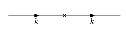
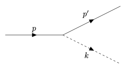
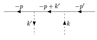
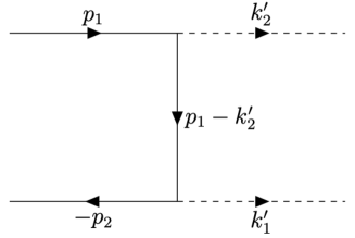
Then, we obtain
| (3.34) |
This gives the contribution of the Fourier transform of the diagram of Figure.1.

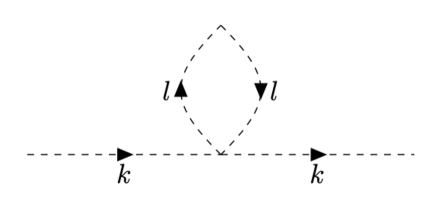
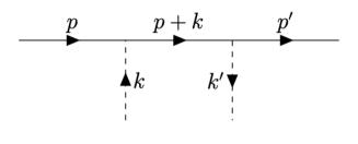
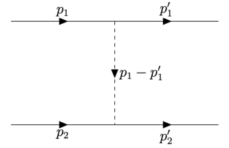
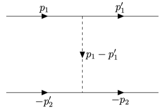
In the same way, we obtain
| (3.35) |
where we omit the spinor indices. This gives the contribution of the Fourier transform of the diagram of Figure.2.
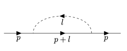
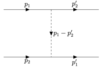
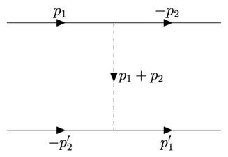
Let us consider the third term in (3.32). This can be calculated as follows:
| (3.36) |
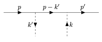
Then, we obtain
| (3.37) |
This gives the contribution of the Fourier transform of the diagram of Figure.3.
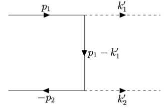
Let us consider the fourth term in (3.32). This can be calculated as follows:
| (3.38) |
where
| (3.39) |
| (3.40) |
and
| (3.41) |
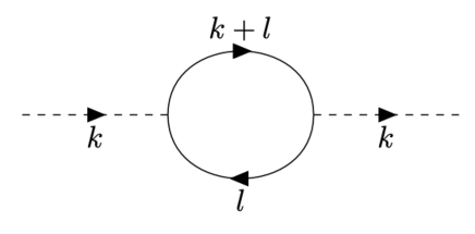
As we will discuss later, the function contributes to and contributes to . The contribution vanishes due to the regularization as in the scalar field theory. 888Here, we do not write down explicitly because this term is the contribution to
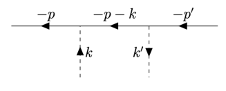
, which we do not calculate here. Then, we obtain
| (3.42) |
This gives the contribution of the Fourier transform of the diagram of Figure.4.
In the same way, we obtain
| (3.43) |
This gives the contribution of the Fourier transformation of the diagram of Figure.5.
The fifth term in (3.32) vanishes from the same reason as the one-point function of the scalar field vanishes due to the regularization as in the scalar field theory.
Therefore, we have reproduced the one-loop two-point functions of the modified Yukawa theory using quantum algebras.
4 The Schwinger-Dyson equations
In this section, we show that the correlation functions of general scalar-Dirac systems described by quantum algebras satisfy the Schwinger-Dyson equations. In this section, we consider scalar fields and Dirac fields in general dimension . In [27], formal degree-odd spinors are introduced and we can prove correlation functions of Dirac fields of any orderings. We can use the same method as the previous paper. In this paper, however, we only consider the correlation functions of the form
| (4.1) |
Correlation functions of different orderings can be proved similarly.
| (4.2) |
where
| (4.3) |
Since
| (4.4) |
| (4.5) |
and
| (4.6) |
we can derive the three types of the Schwinger-Dyson equations. We should show that the Schwinger-Dyson equations derived from (4.4)-(4.6) are satisfied in terms of algebras. In this paper, we show the case of (4.5). The others can be shown similarly. From the equation (4.5), we obtain the following Schwinger-Dyson equations:
| (4.7) |
Here, we can take without the loss of generality. In the path integral formalism, this follows from the Wick’s theorem, and in the formalism using algebras, this follows from the property of . Let us confirm that correlation functions described in terms of quantum algebras satisfy the Schwinger-Dyson equations. The proof of the free part is essentially the same as in [27], so in this paper, we mainly discuss how to deal with interaction terms. First, we rewrite the functional derivative of the action in terms of algebras. After the variation, we obtain
| (4.8) |
We consider following :
| (4.9) |
where
| (4.10) |
| (4.11) |
| (4.12) |
We write the terms which is proportional to in as . We consider the term
| (4.13) |
Suppose that this contains Dirac fields . Then, this contains Dirac adjoint and we obtain
| (4.14) |
We define the operation by the following relation:
| (4.15) |
If
| (4.16) |
we define
| (4.17) |
Therefore, we obtain
| (4.18) |
where the sum denote the all possible sum over and .
Up to this point, we finished the preparation. From the identity
| (4.19) |
and the property
| (4.20) |
for , we have
| (4.21) |
for , where . Then, we obtain
| (4.22) |
Following the proof in [27], we obtain
| (4.23) |
and
| (4.24) |
Therefore, we analyze the following term:
| (4.25) |
Notice that
| (4.26) |
We can write the terms which contributes (4.25) in as follows:
| (4.27) |
where the coefficients of the basis vectors of are all degree even. After a long but straightforward calculation, we obtain
| (4.28) |
Then, equation (4.22) becomes
| (4.29) |
We then acts the operator to find
| (4.30) |
We define
| (4.31) |
and
| (4.32) |
Then,
| (4.33) |
Therefore, we obtain
| (4.34) |
Then, we can derive the following equation:
| (4.35) |
These are exactly the Schwinger-Dyson equations. We have shown that the correlation functions of general scalar-Dirac systems described by algebra satisfy Schwinger-Dyson equations.
5 Conclusions and Discussions
In this paper, we extend the result [27] to general scalar-Dirac systems. The formula presented in the previous paper is given by
| (5.1) |
where
| (5.2) |
For a scalar field , is given by
| (5.3) |
and for a Dirac field , is given by
| (5.4) |
Combining the above, we obtain
| (5.5) |
In this paper, we have shown that the formula (5.1) holds in general scalar-Dirac systems. We would extend this formalism to the other types of fermions such as Majorana fields.
As we discussed in the previous paper, in spite of the asymmetric construction of , has turned out to be totally symmetric for bosonic fields and totally antisymmetric for fermionic fields. It is surprising that this property holds for the interaction theories. This should be directly proved using the techniques of coalgebra representations of algebras and we will try to prove this in future work.
Most of the discussions and future directions are discussed in the previous paper, so see [27] in detailed discussions. We briefly state them.
One future direction is mathematical one. It would be important to discuss the relation to the approach developed by Costello and Gwilliam using factorization algebras [36, 37]. This would contribute to reveal mathematical nature of quantum field theory.
The other direction is to generalize our approach based on algebras to open superstring field theory. For instance, it is discussed in [38] that the expansion of correlation functions of gauge-invariant operators in open superstring field theory is important in the program of providing a framework to prove the AdS/CFT correspondence, but correlation functions have not been discussed much in string field theory.999 See recent papers [39, 40] for interesting progress which will be relevant to this topic. It would also be intriguing to consider the twisted holography [41, 42, 43] from our perspective, and see [44] for recent research.
We hope that this work will contribute to the understanding of the mathematical nature of quantum field theory and the quantization of open string field theory.
Acknowledgments
We wish to thank you for Yuji Okawa for fruitful discussions.
Appendix A Yukawa theory
In this paper, we use string-field-theory-like expressions to express quantum field theory in terms of algebras. In this formalism, we will calculate the tree-level scattering amplitudes of the Yukawa theory101010Calculations of the tree-level amplitudes of Yukawa theory in the path integral formalism are presented, for example, in section 45 of [35]. using algebras.
First, we denote some notations. The free Dirac fields in dimensions can be expanded as
| (A.1) |
where
| (A.2) |
| (A.3) |
and are complex numbers, and and are four-component vectors. The complex numbers corresponds to annihilation operators of electrons and positrons, respectively after the canonical quantization.
A.1 Action
We consider an action
| (A.4) |
Since we only consider tree-level amplitudes, we omit the renormalization parameters. Again, we consider the vector space
| (A.5) |
and we rewrite this action to the form
| (A.6) |
where in is expanded as
| (A.7) |
The definitions of are the same as in the previous sections. We define as
| (A.8) |
to obtain
| (A.9) |
We thus obtain the action of the Yukawa theory in terms of quantum algebras.
A.2 Tree-level scattering amplitudes
It is known that the -point scattering amplitude is calculated in terms of algebras by the following formula:111111See for example [14, 22]. See also [45] for the comprehensive review.
| (A.10) |
where
| (A.11) |
| (A.12) |
is the n-th order symmetry group, and is its permutation. In this case, we need to consider different contracting homotopy from the previous sections. To calculate scattering amplitudes, we consider the on-shell projector . Using this projector, we define
| (A.13) |
These definitions satisfy the Hodge-Kodaira decomposition and the annihilation conditions
| (A.14) |
Then, we have defined all ingredients to calculate the amplitudes.
First, we consider 3-point amplitude . This amplitude can be calculated by considering
| (A.15) |
We take , , as
| (A.16) | ||||
| (A.17) | ||||
| (A.18) |
where we introduced degree-odd parameters and . Note that the amplitudes become the coefficient of degree-odd parameters. In this paper, we do not distinguish amplitudes multiplied by degree-odd parameters and true amplitudes.121212In general, amplitudes contains sign ambiguity. The motivation we introduce the degree-odd parameters is to relate the Lehmann-Symanzik-Zimmermann (LSZ) reduction formula and homotopy algebraic calculations. We conjecture that the ordering of degree-odd parameters corresponds to the ordering of the creation-annihilation operators in the LSZ reduction formula. From the definition (A.11), we obtain
| (A.19) |
Let us calculate the first term in (A.15). From the result (A.19), we obtain
| (A.20) |
We need to care about the sign factors when we calculate .
| (A.21) |
Then, we obtain
| (A.22) |
We can calculate in the same way, and we find
| (A.23) |
Then, we obtain
| (A.24) |
Finally, if we substitute (A.16) and (A.22) into the above, we obtain
| (A.25) |
This completely agrees with the result using the Feynman diagram (Figure 6).
Next, let us calculate 4-point amplitudes . The amplitudes can be calculated from following formula:
| (A.26) |
From the definition (A.11), we can calculate as follows:
| (A.27) |
First, we consider the 4-point amplitude . If we define as follows,
| (A.28) | ||||
| (A.29) | ||||
| (A.30) | ||||
| (A.31) |
where and are degree-odd parameters, then we obtain
| (A.32) |
This completely agrees with the result using the Feynman diagram (Figure 8, 8).
Second, we consider the 4-point amplitude . If we define as follows,
| (A.33) | ||||
| (A.34) | ||||
| (A.35) | ||||
| (A.36) |
where and are degree-odd parameters, then we obtain
| (A.37) |
This completely agrees with the result using the Feynman diagram (Figure 10, 10).
Third, we consider the 4-point amplitude . If we define as follows,
| (A.38) | ||||
| (A.39) | ||||
| (A.40) | ||||
| (A.41) |
where and are degree-odd parameters, then we obtain
| (A.42) |
This completely agrees with the result using the Feynman diagram (Figure 12, 12).
Fourth, we consider the 4-point amplitude . If we define as follows,
| (A.43) | ||||
| (A.44) | ||||
| (A.45) | ||||
| (A.46) |
where and are degree-odd parameters, then we obtain
| (A.47) |
This completely agrees with the result using the Feynman diagram (Figure 14, 14).
Finally, we consider the 4-point amplitude . If we define as follows,
| (A.48) | ||||
| (A.49) | ||||
| (A.50) | ||||
| (A.51) |
where and are degree-odd parameters, then we obtain
| (A.52) |
This completely agrees with the result using the Feynman diagram (Figure 16, 16).
References
- [1] J. D. Stasheff, “Homotopy associativity of -spaces. I,” Trans. of the Amer. Math. Soc. 108, 275 (1963).
- [2] J. D. Stasheff, “Homotopy associativity of -spaces. II,” Trans. of the Amer. Math. Soc. 108, 293 (1963).
- [3] E. Getzler and J. D. S. Jones, “-algebras and the cyclic bar complex,” Illinois J. Math 34, 256 (1990).
- [4] M. Markl, “A cohomology theory for -algebras and applications,” J. Pure Appl. Algebra 83, 141 (1992).
- [5] M. Penkava and A. S. Schwarz, “ algebras and the cohomology of moduli spaces,” hep-th/9408064.
- [6] M. R. Gaberdiel and B. Zwiebach, “Tensor constructions of open string theories. 1: Foundations,” Nucl. Phys. B505, 569 (1997) [hep-th/9705038].
- [7] B. Zwiebach, “Closed string field theory: Quantum action and the Batalin-Vilkovisky master equation,” Nucl. Phys. B 390, 33-152 (1993) [arXiv:hep-th/9206084 [hep-th]].
- [8] M. Markl, “Loop homotopy algebras in closed string field theory,” Commun. Math. Phys. 221, 367-384 (2001) [arXiv:hep-th/9711045 [hep-th]].
- [9] A. Sen, “Wilsonian Effective Action of Superstring Theory,” JHEP 01, 108 (2017) [arXiv:1609.00459 [hep-th]].
- [10] H. Erbin, C. Maccaferri, M. Schnabl and J. Vošmera, “Classical algebraic structures in string theory effective actions,” JHEP 11, 123 (2020) [arXiv:2006.16270 [hep-th]].
- [11] D. Koyama, Y. Okawa and N. Suzuki, “Gauge-invariant operators of open bosonic string field theory in the low-energy limit,” [arXiv:2006.16710 [hep-th]].
- [12] A. S. Arvanitakis, O. Hohm, C. Hull and V. Lekeu, “Homotopy Transfer and Effective Field Theory I: Tree-level,” Fortsch. Phys. 70, no.2-3, 2200003 (2022) [arXiv:2007.07942 [hep-th]].
- [13] A. S. Arvanitakis, O. Hohm, C. Hull and V. Lekeu, “Homotopy Transfer and Effective Field Theory II: Strings and Double Field Theory,” Fortsch. Phys. 70, no.2-3, 2200004 (2022) [arXiv:2106.08343 [hep-th]].
- [14] H. Kajiura, “Noncommutative homotopy algebras associated with open strings,” Rev. Math. Phys. 19, 1-99 (2007) [arXiv:math/0306332 [math.QA]].
- [15] S. Konopka, “The S-Matrix of superstring field theory,” JHEP 11, 187 (2015) [arXiv:1507.08250 [hep-th]].
- [16] H. Kunitomo, “Tree-level S-matrix of superstring field theory with homotopy algebra structure,” JHEP 03, 193 (2021) [arXiv:2011.11975 [hep-th]].
- [17] T. Erler and H. Matsunaga, “Mapping between Witten and lightcone string field theories,” JHEP 11, 208 (2021) [arXiv:2012.09521 [hep-th]].
- [18] O. Hohm and B. Zwiebach, “ Algebras and Field Theory,” Fortsch. Phys. 65, no.3-4, 1700014 (2017) [arXiv:1701.08824 [hep-th]].
- [19] B. Jurčo, L. Raspollini, C. Sämann and M. Wolf, “-Algebras of Classical Field Theories and the Batalin-Vilkovisky Formalism,” Fortsch. Phys. 67, no.7, 1900025 (2019) [arXiv:1809.09899 [hep-th]].
- [20] A. Nützi and M. Reiterer, “Amplitudes in YM and GR as a Minimal Model and Recursive Characterization,” Commun. Math. Phys. 392, no.2, 427-482 (2022) [arXiv:1812.06454 [math-ph]].
- [21] A. S. Arvanitakis, “The -algebra of the S-matrix,” JHEP 07, 115 (2019) [arXiv:1903.05643 [hep-th]].
- [22] T. Macrelli, C. Sämann and M. Wolf, “Scattering amplitude recursion relations in Batalin-Vilkovisky–quantizable theories,” Phys. Rev. D 100, no.4, 045017 (2019) [arXiv:1903.05713 [hep-th]].
- [23] B. Jurčo, T. Macrelli, C. Sämann and M. Wolf, “Loop Amplitudes and Quantum Homotopy Algebras,” JHEP 07, 003 (2020) [arXiv:1912.06695 [hep-th]].
- [24] C. Saemann and E. Sfinarolakis, “Symmetry Factors of Feynman Diagrams and the Homological Perturbation Lemma,” JHEP 12, 088 (2020) [arXiv:2009.12616 [hep-th]].
- [25] M. Doubek, B. Jurčo and J. Pulmann, “Quantum Algebras and the Homological Perturbation Lemma,” Commun. Math. Phys. 367, no.1, 215-240 (2019) [arXiv:1712.02696 [math-ph]].
- [26] T. Masuda and H. Matsunaga, “Perturbative path-integral of string fields and the structure of the BV master equation,” PTEP 2022, no.11, 113B04 (2022) [arXiv:2003.05021 [hep-th]].
- [27] K. Konosu and Y. Okawa, “Correlation functions involving Dirac fields from homotopy algebras I: the free theory,” [arXiv:2305.11634 [hep-th]].
- [28] O. Gwilliam and T. Johnson-Freyd, “How to derive Feynman diagrams for finite-dimensional integrals directly from the BV formalism,” [arXiv:1202.1554 [math-ph]].
- [29] C. Chiaffrino, O. Hohm and A. F. Pinto, “Homological Quantum Mechanics,” [arXiv:2112.11495 [hep-th]].
- [30] I. A. Batalin and G. A. Vilkovisky, “Gauge Algebra and Quantization,” Phys. Lett. B 102, 27-31 (1981).
- [31] I. A. Batalin and G. A. Vilkovisky, “Quantization of Gauge Theories with Linearly Dependent Generators,” Phys. Rev. D 28, 2567-2582 (1983) [erratum: Phys. Rev. D 30, 508 (1984)].
- [32] A. S. Schwarz, “Geometry of Batalin-Vilkovisky quantization,” Commun. Math. Phys. 155, 249-260 (1993) [arXiv:hep-th/9205088 [hep-th]].
- [33] M. Dimitrijević Ćirić, N. Konjik, V. Radovanović and R. J. Szabo, “Braided Quantum Electrodynamics,” [arXiv:2302.10713 [hep-th]].
- [34] Y. Okawa, “Correlation functions of scalar field theories from homotopy algebras,” [arXiv:2203.05366 [hep-th]].
- [35] M. Srednicki, “Quantum Field Theory,” Cambridge University Press (2007).
- [36] K. Costello and O. Gwilliam, “Factorization Algebras in Quantum Field Theory: Volume 1,” Cambridge University Press (2016).
- [37] K. Costello and O. Gwilliam, “Factorization Algebras in Quantum Field Theory: Volume 2,” Cambridge University Press (2021).
- [38] Y. Okawa, “Nonperturbative definition of closed string theory via open string field theory,” based on the talk at International Conference on String Field Theory and String Perturbation Theory held at The Galileo Galilei Institute for Theoretical Physics (Florence, May of 2019) [arXiv:2006.16449 [hep-th]].
- [39] C. Maccaferri, A. Ruffino and J. Vošmera, “The Nilpotent Structure of Open-Closed String Field Theory,” [arXiv:2305.02843 [hep-th]].
- [40] C. Maccaferri, A. Ruffino and J. Vošmera, “Open-Closed String Field Theory in the Large Limit,” [arXiv:2305.02844 [hep-th]].
- [41] K. Costello and S. Li, “Twisted supergravity and its quantization,” [arXiv:1606.00365 [hep-th]].
- [42] K. Costello, “Holography and Koszul duality: the example of the brane,” [arXiv:1705.02500 [hep-th]].
- [43] K. Costello and D. Gaiotto, “Twisted Holography,” [arXiv:1812.09257 [hep-th]].
- [44] K. Zeng, “Twisted Holography and Celestial Holography from Boundary Chiral Algebra,” [arXiv:2302.06693 [hep-th]].
- [45] T. Macrelli, “Homotopy algebras, gauge theory, and gravity,” doi:10.15126/thesis.900068