Analyzing the Shuffle Model through the Lens of Quantitative Information Flow

Abstract

Local differential privacy (LDP) is a variant of differential privacy (DP) that avoids the necessity of a trusted central curator, at the expense of a worse trade-off between privacy and utility. The shuffle model has emerged as a way to provide greater anonymity to users by randomly permuting their messages, so that the direct link between users and their reported values is lost to the data collector. By combining an LDP mechanism with a shuffler, privacy can be improved at no cost for the accuracy of operations insensitive to permutations, thereby improving utility in many analytic tasks. However, the privacy implications of shuffling are not always immediately evident, and derivations of privacy bounds are made on a case-by-case basis.

In this paper, we analyze the combination of LDP with shuffling in the rigorous framework of quantitative information flow (QIF), and reason about the resulting resilience to inference attacks. QIF naturally captures (combinations of) randomization mechanisms as information-theoretic channels, thus allowing for precise modeling of a variety of inference attacks in a natural way and for measuring the leakage of private information under these attacks. We exploit symmetries of the particular combination of $k$-RR mechanisms with the shuffle model to achieve closed formulas that express leakage exactly. In particular, we provide formulas that show how shuffling improves protection against leaks in the local model, and study how leakage behaves for various values of the privacy parameter of the LDP mechanism.

In contrast to the strong adversary from differential privacy, who knows everyone’s record in a dataset but the target’s, we focus on an uninformed adversary, who does not know the value of any individual in the dataset. This adversary is often more realistic as a consumer of statistical datasets, and indeed we show that in some situations mechanisms that are equivalent w.r.t. the strong adversary can provide different privacy guarantees under the uninformed one. Finally, we also illustrate the application of our model to the typical strong adversary from DP.

I Introduction

Differential privacy (DP), introduced by Dwork and her colleagues [1, 2], is one of the most successful frameworks for privacy protection. The original definition, which is now called central DP, assumes the existence of a trusted curator who has access to the raw user data and is in charge of receiving queries to this data and reporting the corresponding answers, suitably obfuscated so to make them essentially insensitive to any single data point. Differential privacy provides formal privacy guarantees and has various desirable properties, such as compositionality, which ensure its robustness to repeated queries. However, the fact that all user data is in the hands of one party means that there is a single point of failure: the privacy of all users depends on the integrity of the curator, and on his capability to protect them from security breaches.

As an alternative to the central model, researchers have proposed local differential privacy (LDP) [3, 4], which does not require a trustworthy data curator. In this model, each user applies an LDP-compliant protocol to perturb her data on the client side and sends it to an aggregator. Then, an analyst can estimate the desired query based on the collected noisy data from all users on the server side. The result is guaranteed to be private due to the postprocessing property. LDP has become very popular, partially thanks to its adoption by tech giants such as Google [5, 6], Apple [7, 8], and Microsoft [9], that have deployed LDP-compliant algorithms into their products to collect users’ usage statistics.

In comparison with central DP, however, LDP suffers from a worse trade-off between privacy and utility. Namely, in order to achieve the same accuracy as in the central model, we need either to lower the level of individual protection, or to provide more data samples. Indeed, there are a number of lower bounds on the error of locally private protocols that strongly separate the local and the central model [10, 11].

The respective drawbacks of the central and the local model have stimulated the search for different architectures, and in this context, the shuffle model [12] has emerged as an appealing alternative. This model, in its simplest form, assumes a data collector who receives one message from each of the users, as in LDP. In contrast to the latter, however, it also assumes that a mechanism is in place to randomly permute the messages , before they reach the data collector, so that any direct association between users and their reported values is lost. In this way, shuffling provides privacy amplification at no cost for the utility for the accuracy of commutative operations, i.e., operations that are insensitive to the order of data. These correspond to a large class of the most typical analytical tasks, such as sum, average, and histogram queries. In this way, the trade-off between privacy and utility is substantially improved for those queries, and in some cases, it even becomes very close to that of the central model [13].

Research on the shuffle model has focused on finding bounds for the level of privacy obtained after shuffling, expressed in terms of the privacy parameter (or parameters, in case of approximate LDP) of the local obfuscation mechanism used in combination with the shuffler. These bounds have been improved, i.e., made stricter over the years, but the proofs are quite involved and produced in a case-by-case basis, without a unifying framework to reason about inference attacks against the shuffle model altogether.

In this paper, we take a different perspective by analyzing the shuffle model from the point of view of quantitative information flow (QIF) [14], which is a rigorous framework grounded on sound information– and decision-theoretic principles to reason about the leakage caused by inference attacks. QIF has been successfully applied to a variety of privacy and security analyses, including searchable encryption [15], intersection and linkage attacks against $k$-anonymity [16] and very large, longitudinal microdata collections [17], and differential privacy [18, 19].

In the QIF framework, a system is modeled as information-theoretic channel taking in some secret input and producing some observable output. The information leakage is defined as the difference between the vulnerability of the secret (i.e., the amount of useful information to perform an attack) before and after passing through the channel (prior and posterior vulnerabilities , respectively). The vulnerability, indeed, increases because the attacker can infer information about the input by observing the output. The vulnerability measure also depends on the adversary’s goals and capabilities , which are captured in the state-of-the-art QIF framework of $g$-leakage [20] by using suitable gain functions. We model both the shuffler and the LDP mechanism as information-theoretic channels, and their composition with the operation of channel cascading, and we study their leakage. In this paper, we understand vulnerability as the adversary’s ability to infer personal data, and can thereby be considered the inverse of privacy; i.e., the higher the vulnerability, the lower the privacy, and vice-versa.

We examine the single-message shuffle model protocols, in which each user sends a single data point to the collector, and also on the $k$-ary randomized response ($k$-RR) mechanism [21] which is one of the most popular mechanisms for LDP, and the core of Google’s RAPPOR [5]. We focus on the case in which the goal of the adversary is to guess the secret value of a single individual (target) from the dataset, which corresponds to the typical scenario of differential privacy in which the reported answer should not allow an observer to distinguish with confidence between two adjacent datasets [22, 23, 24, 25]. 

A key distinction of our work, however, is that we focus on an uninformed adversary, who does not know anyone’s values before accessing a data release, and assumes a uniform prior on datasets. It is well known from the literature that the guarantees against inferences provided by differential privacy hold only w.r.t.  what is usually called the strong adversary, who knows everyone’s data except those of the target individual. However, adversaries with weaker, less informed priors, can often benefit more from an inference attack than the strong adversary, simply because there is more to be learned by them [22, 23, 24, 25]. The fact that differential privacy’s guarantees against a strong adversary do not necessarily carry over to less knowledgeable adversaries is commonly overlooked in some interpretations of the framework.   We refer to recent work by Tschantz et al. [22] for an excellent presentation of the issue. Another important reason to study the uninformed adversary is that it is more realistic, as usually in DP consumers cannot access the micro-data directly. This is important if we want to compare mechanisms for privacy: it could be the case that two mechanisms $M$ and $M^{\prime}$ are equivalent under the strong adversary, but they are not under the uninformed adversary. For example, assume for simplicity that each record contains one bit, and that $M$ outputs the last bit (i.e., the content of the last record) in the dataset, or its complement, with probabilities $\nicefrac{{e^{\epsilon}}}{{1+e^{\epsilon}}}$ and $\nicefrac{{1}}{{1+e^{\epsilon}}}$, respectively. In contrast, $M^{\prime}$ computes the binary sum of the other bits, and behaves exactly as $M$ if this sum is $0$, otherwise, it outputs the same last bit or its complement, but with inverted probabilities w.r.t. what $M$ does. It is easy to see that both $M$ and $M^{\prime}$ are exactly $\epsilon$-differentially private, so they are equivalent under the strong adversary (who knows all the records except the last one), but $M^{\prime}$ is more private than $M$ under the uninformed adversary. More specifically, in $M^{\prime}$ the reported value does not give any information on the original value of the last record (the posterior probability of it being $0$ or $1$ are the same, as in the prior), whereas in $M$ some information is gained.

In any case, once we have a QIF model for LDP and shuffle, the same techniques can be applied to derive results about their information leakage properties of other variants of adversaries.

We investigate extensively the binary case, i.e., when $k=2$. Despite its simplicity, the binary case is quite ubiquitous, and deserves special attention. Databases often contain binary attributes, modeling the presence or absence of a given feature or storing “yes” or “no” answers to sensitive questions. Indeed, randomized response was developed as a survey technique motivated by the need to collect binary responses [26]. Successively, we extend our investigation to a generic $k$.

I-A Contribution

Our contributions are the following:

• We study the information leakage of different combinations of $k$-RR and of the shuffler (Section III). To the best our knowledge, this is the first formal QIF model for the combination of LDP and shuffle mechanisms. In particular, we prove that they commute, i.e., that it is equivalent (w.r.t. leakage) to first apply $k$-RR and then the shuffler, or to do the opposite (Proposition 11). 

• We investigate leakage under uninformed adversaries for $k{=}2$ (Section IV), and derive the first exact, closed formulas for posterior vulnerability, and therefore for leakage (Theorems 17 and 19).

• We investigate leakage under uninformed adversaries for generic values $k{\geq}2$ (Section VI). Although we derive the first formulas for the vulnerabilities in this case (Propositions 20 and 21), they are neither closed nor computationally efficient. Nevertheless, we are able to provide novel asymptotic bounds on leakage (Theorem 20) by uncovering a surprising connection between our scenario of interest and a well-known combinatoric problem.

• We use the above formulas to study leakage as the size of the dataset increases, for various privacy parameters of $k$-RR (Sections IV-B, VI-B and VI-C).

• We provide a brief discussion on how our QIF model, being parametric on the adversary’s prior knowledge, can be used to reason about the strong adversary from differential privacy (Section V).

• We show that in the case of uninformed adversaries, shuffling is much more effective than noise for leakage reduction, hence the best trade-off between privacy and utility may be obtained by using the shuffling alone. In contrast, in the case of the strong adversary, noise obfuscation plays a crucial role in privacy protection, hence the best trade-off is achieved by combining noise and shuffling (Sections IV and VI).

I-B Related Work

The shuffle model was the core idea in the Encode, Shuffle, Analyze (ESA) model introduced by Bittau et al. [12] (see also [28] for a revised version of that work). Cheu et al.  [13] formalized the definition of the shuffle model and also provided the first separation result showing that the shuffle model is strictly between the central and the local models of DP. Characterizing the exact nature of this separation has been the aim of many subsequent works. Erlingsson et al. [29] showed that the introduction of a trusted shuffler amplifies the privacy guarantees against an adversary who is not able to access the outputs from the local randomisers but only sees the shuffled output. Balle et al. [27] improved and generalized the results by Erlingsson et al. to a wider range of parameters, and provided a family of methods to analyze privacy amplification in the shuffle model. Feldman et al. [30] developed a similar concept of “hiding in the crowd”, and suggested an asymptotically optimal dependence of the privacy amplification on the privacy parameter of the local randomizer. Koskela et al. [31, 32] proposed a numerical approach (i.e., not expressed by an analytical formula) to estimate tight bounds based on weak adversaries.

Other directions of research related to shuffle models address summation queries [33, 34, 13, 35, 36, 37] and histogram queries [38, 39]. Balle et al. [27] proposed a single-message protocol for messages in the interval $[0,1]$, and Cheu et al. [13] conducted a study on a bounded real-valued statistical queries using additional communication costs. Ishai et al. [35] analyzed a protocol that reduced the number of messages in the summation query under shuffle models, and Balcer et al. [38] proposed a shuffle mechanism for histogram queries.

Further relevant work involves robust shuffle differential privacy [40, 41, 42]. Shuffle models can provide a targeted level of privacy protection only with at least a specific number of users participating in the shuffle. If the number of data providers does not reach a certain quantity, the level of privacy protection degrades. Thus, studies on robust shuffle differential privacy have gained recent attention in the community. Balcer et al. [40] explores robust shuffle private protocols and suggests a relationship between robust shuffle privacy and pan-privacy.

Connections between QIF and differential privacy have been explored in the literature. Barthe and Köpf [43] relate centralized differential privacy and information-theoretic notions of leakage, establishing bounds on the former in terms of the value of $\epsilon$. In a similar line of work, Alvim et al. [18] employ QIF to analyze leakage and utility in oblivious, centralized differentially-private mechanisms. They improve some of the bounds by Barthe and Köpf, and provide a mechanism that, if some constraints are satisfied, maximizes utility for a given level of differential privacy. Both of these works, however, focus on the centralized model of differential privacy (rather than on the local model, as we do), and do not consider shuffling at all. Chatzikokolakis et al. [44] investigate leakage orderings induced by different differential privacy mechanisms, but, again, do not consider shuffling. To the best of our knowledge, our work is the first to provide a QIF analysis of the combination of locally differentially-privacy and shuffle mechanisms. Moreover, we provide closed formulas (rather than bounds) to compute leakage in practical scenarios.

I-C Plan of the paper

In Section II, we review fundamentals from QIF, LDP, $k$-RR, and the shuffle model. In Section III, we provide a QIF model for $k$-RR and the shuffler as channels and investigate different combinations of such channels. In Section IV, we study leakage under an adversary with a uniform prior over datasets focusing on a single target, for $k{=}2$. In Section V, we briefly consider the typical strong adversary from differential privacy also for $k{=}2$. In Section VI, we extend our investigation from Section IV to generic values of $k{\geq}2$. In Section VII, we present consequences of our findings, and in Section VIII, we conclude.

II Preliminaries

Firstly, we review the analytical framework of quantitative information flow. While we introduce fundamental notation and vocabulary, the definitive resource on quantitative information flow with definitions, theorems, and proofs can be found in [14]. Secondly, we review $k$-RR local differential privacy along with the shuffle model. Readers familiar with both fields should feel free to move to the following section.

II-A QIF

The quantitative information flow (QIF) framework captures the adversary’s knowledge, goals, and capabilities, and from that, quantifies the leakage of information caused by a corresponding optimal inference attack. The framework is grounded on sound information– and decision-theoretic principles enabling the rigorous assessment of how much information leakage a system allows in principle, and independently from the adversary’s computational power [45, 46, 47, 14]. Hence, QIF guarantees hold no matter the particular tactic or algorithm the adversary employs to execute the attack, as what is measured is exactly how much sensitive information is leaked by the best possible such tactic or algorithm.

QIF separates (1) the adversary’s knowledge (modeled as a prior distribution on secret values) from (2) her intentions and capabilities (modeled as a gain function), and that is separated from (3) the description of the system being run (modeled as an information-theoretic channel). We describe these components in more detail now.

QIF assumes the input has a probability distribution $\pi$ that is known to an adversary. We denote the random variables associated with the channel’s input and output as $X$ and $Y$, respectively. The system is modeled as a channel matrix C, where $\textnormal{{C}}_{x,y}$ contains the conditional probability $Pr(y\mid x)$. We assume the adversary knows how the channel works as well as the entries in $\textnormal{{C}}_{x,y}$. Knowing the distribution on secrets and the channel matrix, she can update her knowledge about $X$ to a posterior distribution $Pr(x\mid y)$. Since each output $y$ also has a probability $Pr(y)$, the channel matrix C provides a mapping from any prior $\pi$ to distributions on posterior distributions, which we call a hyper-distribution and denote $[\pi\triangleright\textnormal{{C}}]$.

There is no one “right” way to measure how a system affects a secret since the adversary’s probability of success depends on their goals and operational context. To address this, QIF uses the $g$-leakage framework, introduced by [20]. This framework defines the vulnerability of secret $X$ with respect to specific operational scenarios. An adversary is given a set $\mathcal{W}$ of actions (or guesses) that she can make about the secret, and given a gain function $g(w,x)$ ranging over non-negative reals which defines the gain of selecting the action $w$ when the real secret is $x$.  An optimal adversary will choose an action that maximizes her expected gain with respect to $\pi$. The gain function then determines a secret’s vulnerability.

Given a prior distribution on secrets $\pi$, prior $g$-vulnerability, denoted $V_{g}(\pi)$, represents the adversary’s expected gain of her optimal action based only on $\pi$, i.e., before observing the channel output.

Definition 1 (Prior vulnerability).

Given a prior $\pi$ and a gain function $g$, the corresponding prior vulnerability is given by

$$\mathit{V_{g}(\pi)\vcentcolon=\max_{w\in\mathcal{W}}\sum_{x\in\mathcal{X}}\pi_{x}\cdot g(w,x)}\,.$$ (1)

In the posterior case, the adversary observes the output of the system which allows her to improve her action and consequent expected gain.

Definition 2 (Posterior vulnerability).

Given a prior $\pi$, a gain function $g$, and channel matrix C from $\mathcal{X}$ to $\mathcal{Y}$, the corresponding posterior vulnerability is given by

$$V_{g}[\pi\triangleright\textnormal{{C}}]\vcentcolon=\sum_{y\in\mathcal{Y}}\max_{w\in\mathcal{W}}\sum_{x\in\mathcal{X}}\pi_{x}\cdot\textnormal{{C}}_{xy}\cdot g(w,x)\,.$$ (2)

The choice of the gain function $g$ covers a vast variety of adversarial scenarios [20]. Indeed, any vulnerability function satisfying a set of basic information-theoretic axioms can be expressed as $V_{g}$ for a properly constructed $g$ [48].

We measure the channel leakage by comparing the prior and posterior $g$-vulnerability, which quantifies how much a specific channel C increases the vulnerability of the system. This comparison can be done additively or multiplicatively. Channel matrices can be large and difficult to evaluate, necessitating simplification. It is interesting, hence, to consider the concept of channel equivalence w.r.t. information leakage properties. Two channels C and $\textnormal{{C}}^{\prime}$ defined on the same input set (but possibly different output sets) are considered equivalent, denoted by $\textnormal{{C}}\equiv\textnormal{{C}}^{\prime}$, iff, for all priors $\pi$ on their input set and gain function $g$, their posterior vulnerabilities are the same, i.e., $V_{g}[\pi\triangleright\textnormal{{C}}]=V_{g}[\pi\triangleright\textnormal{{C}}^{\prime}]$. (Notice that if the posterior vulnerabilities for both channels are same, then so will be their corresponding multiplicative and additive leakages, since the channels share the same prior vulnerability.) One way to simplify a channel matrix into an equivalent one is to adjust extraneous structure by deleting output labels and adding similar columns together (columns that are scalar multiples of each other) , since output labels do not affect leakage.

Importantly for this work, channel matrices can compose in cascades such that the output of one channel becomes the input for another. As defined in  [14],

Definition 3 (Channel cascade).

Given channel matrices $\textnormal{{C}}:\mathcal{X}\rightarrow\mathcal{Y}$ and $\textnormal{{D}}:\mathcal{Y}\rightarrow\mathcal{Z}$, the cascade of C and D is the channel matrix CD of type $\mathcal{X}\rightarrow\mathcal{Z}$, where CD is given by ordinary matrix multiplication.

Cascades model sequential operations, where the adversary observes the final output. In the same way that $\textnormal{{C}}_{x,y}$ specifies $Pr(y\mid x)$, a cascade $\textnormal{{CD}}:\mathcal{X}\rightarrow\mathcal{Z}$ specifies $Pr(z\mid x)$. From the perspective of information leakage, cascades have an important operational significance: D here acts as a sanitization policy, suppressing the release of $Y$.

In fact, by the data-processing inequality for the $g$-leakage framework (expressed in Theorem 4 below), for any D in cascade CD, we know that leakage can never be increased. To understand this property, let us define the refinement relation among channels of the same input space as $\textnormal{{C}}\sqsubseteq\textnormal{{C}}^{\prime}$, meaning that C is refined by $\textnormal{{C}}^{\prime}$ (or, equivalently, that $\textnormal{{C}}^{\prime}$ refines C) iff, for all priors $\pi$ on their input set and gain function $g$, their posterior vulnerabilities satisfy $V_{g}[\pi\triangleright\textnormal{{C}}]\geq V_{g}[\pi\triangleright\textnormal{{C}}^{\prime}]$. Then the data-processing inequality for the $g$-leakage framework is established as follows [14].

Theorem 4 (Data-processing inequality).

Given channel matrices $\textnormal{{C}}:\mathcal{X}\rightarrow\mathcal{Y}$ and $\textnormal{{C}}^{\prime}:\mathcal{X}\rightarrow\mathcal{Z}$, we have that $\textnormal{{C}}\sqsubseteq\textnormal{{C}}^{\prime}$ iff there exists a channel matrix $\textnormal{{D}}:\mathcal{Y}\rightarrow\mathcal{Z}$ such that $\textnormal{{C}}\textnormal{{D}}=\textnormal{{C}}^{\prime}$.

II-B Local Differential Privacy (LDP)

Let $\mathcal{K}$ be the set of values for a single individual’s sensitive attribute, and $k$ be the size of $\mathcal{K}$. We say that a mechanism $\mathcal{R}$ is $\epsilon$-LDP if, for all $x,x^{\prime},y\in\mathcal{K}$, we have

$$Pr(\mathcal{R}(x)=y)\leq e^{\epsilon}\;Pr(\mathcal{R}(x^{\prime})=y)\,,$$

where $Pr(a)$ represents the probability of the event $a$ and $e$ is the exponentiation operator.

II-C $k$-ary Randomized Response ($k$-RR)

The $k$-ary Randomized Response with privacy parameter $\epsilon$ is a mechanism $\mathcal{R}$ defined as:

$$Pr(\mathcal{R}(x)=y)=\left\{\begin{array}[]{rl}{\color[rgb]{0,0,0}\nicefrac{{\displaystyle e^{\epsilon}}}{{\displaystyle(k-1+e^{\epsilon})}},}&{\color[rgb]{0,0,0}\text{if $y=x$,}}\\ \\ {\color[rgb]{0,0,0}\nicefrac{{\displaystyle 1}}{{\displaystyle(k-1+e^{\epsilon})}},}&{\color[rgb]{0,0,0}\text{otherwise.}}\end{array}\right.$$ (3)

It is easy to prove that such a mechanism satisfies $\epsilon$-DP [49].

II-D Shuffler, simplified version

We consider only the single-message shuffler model. We can define the shuffler as a mechanism $\mathcal{R}$ that takes as input a tuple of elements of $\mathcal{K}$ of some fixed length $n$, and produces a random permutation of it, with uniform probability. Namely, for all $(x_{0},x_{1},\ldots,x_{n-1})\in\mathcal{K}^{n}$ and all permutations $(y_{0},y_{1},\ldots,y_{n-1})$ of $(x_{0},x_{1},\ldots,x_{n-1})$, we have

$$Pr(\mathcal{R}(x_{0},x_{1},\ldots,x_{n-1})=(y_{0},y_{1},\ldots,y_{n-1}))\;=\;\frac{1}{n!}\;.$$

III QIF model for local differential privacy and shuffling

In this section, we provide a formal model based on the QIF framework for the application of LDP mechanisms and of shuffle mechanisms to datasets containing sensitive values. The model will be instrumental in the next sections, where we investigate information leakage properties of these mechanisms and of their various compositions in different configurations of the adversary’s prior knowledge.

III-A Sensitive values, datasets, and the general scenario

We begin by formalizing the general scenario we consider.

Definition 5 (Sensitive values and datasets).

Let $\mathcal{N}=\{0,1,\ldots,n-1\}$ be a set of $n\geq 1$ individuals of interest, and $\mathcal{K}$ be a set of $k\geq 2$ possible values for each individual’s sensitive attribute. A dataset $x$ is a tuple $(x_{0},x_{1},\ldots,x_{n-1})$ in which each element $x_{i}\in\mathcal{K}$ is the value of the sensitive attribute for individual $i\in\mathcal{N}$. The domain of all possible datasets is, hence, $\mathcal{K}^{n}$, and it has size $k^{n}$.

Moreover, we adopt the following notation and terminology. Given a set $\mathcal{K}=\{\kappa_{0},\kappa_{1},\ldots,\kappa_{k-1}\}$ of values for the sensitive attribute, and a dataset $x\in\mathcal{K}^{n}$, we let

• the tuple $x=(x_{0},x_{1},\ldots,x_{n-1})$ be denoted by the sequence $x_{0}x_{1}\ldots x_{n-1}$ of its elements;

• $n_{\kappa_{j}}(x)$ represent the the number of individuals in the dataset $x$ having sensitive value $\kappa_{j}\in\mathcal{K}$;

• $h(x)=(\kappa_{0}{:}n_{\kappa_{0}}(x),\,\,\kappa_{1}{:}n_{\kappa_{1}}(x),\,\,\ldots,\,\,\kappa_{k-1}{:}n_{\kappa_{k-1}}(x))$ be the the histogram of dataset $x$, containing a list of each possible value $\kappa_{j}\in\mathcal{K}$ followed by the count $n_{\kappa_{j}}(x)$ of individuals in $x$ with that value; and

• $\#h(x)=|\{x^{\prime}\in\mathcal{K}^{n}\mid h(x^{\prime})=h(x)\}|$ be the number of distinct datasets in $\mathcal{K}^{n}$ having the same histogram as $x$.

We consider a dataset $x\in\mathcal{K}^{n}$ containing the real value of the sensitive attribute for all individuals in $\mathcal{N}$. We also assume that a data analyst wants to infer some statistical information about the original dataset (e.g., an average or count), but the dataset’s exact contents –in particular, the link between individuals and their sensitive attribute– are considered secret.

Example 6 (Running example).

Consider a scenario in which there are $n\,{=}\,3$ individuals and a sensitive binary attribute with possible values in $\mathcal{K}=\{\texttt{a},\texttt{b}\}$. The set of all possible datasets is then $\{\texttt{a},\texttt{b}\}^{3}=\{\texttt{a}\texttt{a}\texttt{a},\texttt{a}\texttt{a}\texttt{b},\texttt{a}\texttt{b}\texttt{a},\texttt{a}\texttt{b}\texttt{b},\texttt{b}\texttt{a}\texttt{a},\texttt{b}\texttt{a}\texttt{b},\texttt{b}\texttt{b}\texttt{a},\texttt{b}\texttt{b}\texttt{b}\}.$

III-B Sanitization mechanisms as channels

We consider two sanitization mechanisms which can be employed either individually or in combination. The $k$-RR mechanism is applied to each individual’s sensitive value to introduce uncertainty, while the shuffle mechanism permutes dataset entries to obfuscate the link between each sensitive value and its owner.

The shuffle channel

The full channels of these mechanisms are quite unwieldy. For example, the shuffle mechanism, with the input dataset aab, can output abb, aba, or baa, each with probability $1/3$. Formally, the shuffle randomly permutes the entries to obfuscate the link between each sensitive value and its owner. Abstracting from implementation details and assuming perfect shuffling, each input dataset $x$ has an equal probability $\nicefrac{{1}}{{\#h(x)}}$ of mapping to any of the $\#h(x)$ possible output datasets with the same histogram.

Definition 7 (Full shuffle channel).

Let $\mathcal{N}=\{0,1,\ldots,n-1\}$ be a set of $n\geq 1$ individuals and $\mathcal{K}$ be a set of $k\geq 2$ sensitive values. A full shuffle channel S is a channel from $\mathcal{K}^{n}$ to $\mathcal{K}^{n}$ s.t., for all $x\in\mathcal{K}^{n}$ and $y\in\mathcal{K}^{n}$,

$$\textnormal{{S}}_{x,y}= \,\,\begin{cases}\nicefrac{{1}}{{\#h(x)}},&\text{if $h(y)=h(x)$},\\ 0,&\text{otherwise}.\end{cases}$$

Table I(b) contains the full channel S representing the application of shuffling to the scenario of Example 6.

Conveniently, there are symmetries here that we can exploit to simplify the shuffle channel into something more tractable. Notice that once an input dataset $x$ is shuffled into an output dataset $y$, the position of each element in $y$ no longer identifies its owner, and the only information preserved is $x$’s histogram. For instance, in Table I(b), the columns corresponding to datasets aab, aba, and baa are identical and, from the point of view of the adversary, convey the same information. Hence, these columns can be all merged into a new column that represents only the histogram a:2, b:1 that these datasets share. This motivates the definition of a reduced shuffle channel below, whose output is simply the input dataset’s histogram.

Definition 8 (Reduced shuffle channel).

Let S be a full shuffle channel as per Def. 8. A reduced shuffle channel $\textnormal{{S}}^{r}$ corresponding to S is a channel from $\mathcal{K}^{n}$ to histograms on $\mathcal{K}$ s.t., for all $x\in\mathcal{K}^{n}$ and histogram $z$,

$$\textnormal{{S}}^{r}_{x,z}\,\,\,=\,\,\,\sum_{y\in\mathcal{K}^{n}:h(y)=z}\textnormal{{S}}_{x,y}\,\,\,=\,\,\,\begin{cases}1,&\text{if $h(x)=z$},\\ 0,&\text{otherwise}.\end{cases}$$

Table I(c) contains the channel $\textnormal{{S}}^{r}$ representing the application of reduced shuffle to the scenario of Example 6.

We can be confident that this simplification does not alter our analysis. It is known from QIF literature that merging columns that are multiples of (or identical to) each other does not alter the leakage properties of a channel [14]. The original and resulting channels are equivalent, in the sense that, for every $g$-vulnerability measure and prior distribution on secret values, both yield the same quantification of information leakage. Since $\textnormal{{S}}^{r}$ is obtained from S by merging similar columns, these channels are equivalent.

Proposition 9 (Equivalence between full and reduced shuffle).

Let S be a full shuffle channel as per Def. 7, and $\textnormal{{S}}^{r}$ be the reduced shuffle channel obtained from S as per Def. 8. Then

$$\textnormal{{S}}\equiv\textnormal{{S}}^{r}.$$

The $k$-RR channel

The $k$-RR mechanism independently randomizes the sensitive value of each entry of the dataset, and outputs the resulting dataset. This process does not break the link between any individual and their sensitive value, but creates uncertainty about whether the reported value for each individual is accurate. To simplify notation, we will use $p$ to denote the probability representing that an individual’s sensitive value is reported accurately, i.e., $p=\nicefrac{{e^{\epsilon}}}{{k-1+e^{\epsilon}}}$ (cf. Equation 3), and $\overline{p}$ to represent $1{-}p$, i.e., the probability that the true value is swapped with some other one.

The $k$-RR mechanism can be modeled as a channel that probabilistically maps each input dataset $x\in\mathcal{K}^{n}$ to an output dataset $y\in\mathcal{K}^{n}$ as follows.

Definition 10 ($k$-RR channel).

Let $\mathcal{N}=\{0,1,\ldots,n-1\}$ be a set of $n\geq 1$ individuals and $\mathcal{K}$ be a set of $k\geq 2$ sensitive values. A $k$-RR channel N (for “noise”) with parameter $p\in[\nicefrac{{1}}{{k}},1]$ is a channel from $\mathcal{K}^{n}$ to $\mathcal{K}^{n}$ s.t., for all $x\in\mathcal{K}^{n}$ and $y\in\mathcal{K}^{n}$,

$$\textnormal{{N}}_{x,y}= \,\,\prod_{i=0}^{n-1}Pr(y_{i}\mid x_{i}),$$

where

$$Pr(y_{i}\mid x_{i})=\begin{cases}p,&\text{if $y_{i}=x_{i}$},\\ \nicefrac{{\overline{p}}}{{(k-1)}},&\text{if $y_{i}\neq x_{i}$}\end{cases}$$

Notice that $p$ is at least $\nicefrac{{1}}{{k}}$ so $p\geq\nicefrac{{\overline{p}}}{{(k-1)}}$, indicating that the real sensitive value never has a lower probability to be reported than any other value. Table I(a) contains the full channel N representing the application of a $k$-RR mechanism to the scenario of Example 6.

N	aaa	aab	aba	baa	abb	bab	bba	bbb
aaa	Nc1$p^{3}$	Nc5$p^{2}\overline{p}$	Nc5$p^{2}\overline{p}$	Nc5$p^{2}\overline{p}$	Nc8$p\overline{p}^{2}$	Nc8$p\overline{p}^{2}$	Nc8$p\overline{p}^{2}$	Nc4$\overline{p}^{3}$
aab	Nc5$p^{2}\overline{p}$	Nc1$p^{3}$	Nc8$p\overline{p}^{2}$	Nc8$p\overline{p}^{2}$	Nc5$p^{2}\overline{p}$	Nc5$p^{2}\overline{p}$	Nc4$\overline{p}^{3}$	Nc8$p\overline{p}^{2}$
aba	Nc5$p^{2}\overline{p}$	Nc8$p\overline{p}^{2}$	Nc1$p^{3}$	Nc8$p\overline{p}^{2}$	Nc5$p^{2}\overline{p}$	Nc4$\overline{p}^{3}$	Nc5$p^{2}\overline{p}$	Nc8$p\overline{p}^{2}$
baa	Nc5$p^{2}\overline{p}$	Nc8$p\overline{p}^{2}$	Nc8$p\overline{p}^{2}$	Nc1$p^{3}$	Nc4$\overline{p}^{3}$	Nc5$p^{2}\overline{p}$	Nc5$p^{2}\overline{p}$	Nc8$p\overline{p}^{2}$
abb	Nc8$p\overline{p}^{2}$	Nc5$p^{2}\overline{p}$	Nc5$p^{2}\overline{p}$	Nc4$\overline{p}^{3}$	Nc1$p^{3}$	Nc8$p\overline{p}^{2}$	Nc8$p\overline{p}^{2}$	Nc5$p^{2}\overline{p}$
bab	Nc8$p\overline{p}^{2}$	Nc5$p^{2}\overline{p}$	Nc4$\overline{p}^{3}$	Nc5$p^{2}\overline{p}$	Nc8$p\overline{p}^{2}$	Nc1$p^{3}$	Nc8$p\overline{p}^{2}$	Nc5$p^{2}\overline{p}$
bba	Nc8$p\overline{p}^{2}$	Nc4$\overline{p}^{3}$	Nc5$p^{2}\overline{p}$	Nc5$p^{2}\overline{p}$	Nc8$p\overline{p}^{2}$	Nc8$p\overline{p}^{2}$	Nc1$p^{3}$	Nc5$p^{2}\overline{p}$
bbb	Nc4$\overline{p}^{3}$	Nc8$p\overline{p}^{2}$	Nc8$p\overline{p}^{2}$	Nc8$p\overline{p}^{2}$	Nc5$p^{2}\overline{p}$	Nc5$p^{2}\overline{p}$	Nc5$p^{2}\overline{p}$	Nc1$p^{3}$

(a) The $k$-RR channel N where $p$ is the probability a user responds with their true value, and $\overline{p}=1-p$. Cells are shaded according to the entries’ values when $p=0.75$.

S	aaa	aab	aba	abb	baa	bab	bba	bbb
aaa	1	0	0	0	0	0	0	0
aab	0	$\nicefrac{{1}}{{3}}$	$\nicefrac{{1}}{{3}}$	0	$\nicefrac{{1}}{{3}}$	0	0	0
aba	0	$\nicefrac{{1}}{{3}}$	$\nicefrac{{1}}{{3}}$	0	$\nicefrac{{1}}{{3}}$	0	0	0
abb	0	0	0	$\nicefrac{{1}}{{3}}$	0	$\nicefrac{{1}}{{3}}$	$\nicefrac{{1}}{{3}}$	0
baa	0	$\nicefrac{{1}}{{3}}$	$\nicefrac{{1}}{{3}}$	0	$\nicefrac{{1}}{{3}}$	0	0	0
bab	0	0	0	$\nicefrac{{1}}{{3}}$	0	$\nicefrac{{1}}{{3}}$	$\nicefrac{{1}}{{3}}$	0
bba	0	0	0	$\nicefrac{{1}}{{3}}$	0	$\nicefrac{{1}}{{3}}$	$\nicefrac{{1}}{{3}}$	0
bbb	0	0	0	0	0	0	0	1

(b) Full shuffle channel S which receives datasets as input and produces a datasets as output.

$\textnormal{{S}}^{r}$	a:3, b:0	a:2, b:1	a:1, b:2	a:0, b:3
aaa	1	0	0	0
aab	0	1	0	0
aba	0	1	0	0
abb	0	0	1	0
baa	0	1	0	0
bab	0	0	1	0
bba	0	0	1	0
bbb	0	0	0	1

(c) Reduced shuffle channel $\textnormal{{S}}^{r}$ which receives datasets as inputs and produces histograms as outputs.

TABLE I: Examples of channels for the $k$-RR and shuffling mechanisms, with $k=2$ possible sensitive values and $n=3$ individuals.

III-C The combination of sanitization mechanisms

The sanitization mechanisms presented in the previous section can be applied to an input dataset either in isolation or in combination. In the QIF framework, the effect of this combination is captured by channel cascading (Def. 3). We shall now cover the various possibilities.

We begin by analyzing the typical pipeline used in the literature, which first applies the noisy $k$-RR mechanism to the original dataset, and then applies a shuffle mechanism to the result of the first sanitization [12]. The channel cascade NS mirrors this process: the datasets are processed by N, producing a randomized intermediate dataset, which are taken as input into S which shuffles the entries and produces a final output dataset. The matrix itself can be easily generated by matrix multiplication.

Interestingly, in our scenario the order of application of the full mechanisms N and S is irrelevant, in the sense that the resulting channels will be equivalent w.r.t. the information leakage they cause. This commutativity property is formalized in the following result.

Proposition 11 (Commutativity of $k$-RR and shuffle: Full case).

Let $\mathcal{N}=\{0,1,\ldots,n-1\}$ be a set of $n\geq 1$ individuals and $\mathcal{K}$ be a set of $k\geq 2$ values for the sensitive attribute. Let also N be a $k$-RR channel as per Definition 10, and S be a full shuffle channel per Definition 7. Then

$$\textnormal{{N}}\textnormal{{S}}\equiv\textnormal{{S}}\textnormal{{N}}.$$

Consider again the scenario of Example 6. The channel NS and the channel SN representing the application of $k$-RR followed by full shuffle or vice-versa are identical, as represented in Table II.

NS / SN	aaa	aab	aba	baa	abb	bab	bba	bbb
aaa	NSc1$p^{3}$	NSc5$p^{2}\overline{p}$	NSc5$p^{2}\overline{p}$	NSc5$p^{2}\overline{p}$	NSc8$p\overline{p}^{2}$	NSc8$p\overline{p}^{2}$	NSc8$p\overline{p}^{2}$	NSc4$\overline{p}^{3}$
aab	NSc5$p^{2}\overline{p}$	NSc9$\nicefrac{{1}}{{3}}(p^{3}+2p\overline{p}^{2})$	NSc9$\nicefrac{{1}}{{3}}(p^{3}+2p\overline{p}^{2})$	NSc9$\nicefrac{{1}}{{3}}(p^{3}+2p\overline{p}^{2})$	NSc10$\nicefrac{{1}}{{3}}(2p^{2}\overline{p}+\overline{p}^{3})$	NSc10$\nicefrac{{1}}{{3}}(2p^{2}\overline{p}+\overline{p}^{3})$	NSc10$\nicefrac{{1}}{{3}}(2p^{2}\overline{p}+\overline{p}^{3})$	NSc8$p\overline{p}^{2}$
aba	NSc5$p^{2}\overline{p}$	NSc9$\nicefrac{{1}}{{3}}(p^{3}+2p\overline{p}^{2})$	NSc9$\nicefrac{{1}}{{3}}(p^{3}+2p\overline{p}^{2})$	NSc9$\nicefrac{{1}}{{3}}(p^{3}+2p\overline{p}^{2})$	NSc10$\nicefrac{{1}}{{3}}(2p^{2}\overline{p}+\overline{p}^{3})$	NSc10$\nicefrac{{1}}{{3}}(2p^{2}\overline{p}+\overline{p}^{3})$	NSc10$\nicefrac{{1}}{{3}}(2p^{2}\overline{p}+\overline{p}^{3})$	NSc8$p\overline{p}^{2}$
baa	NSc5$p^{2}\overline{p}$	NSc9$\nicefrac{{1}}{{3}}(p^{3}+2p\overline{p}^{2})$	NSc9$\nicefrac{{1}}{{3}}(p^{3}+2p\overline{p}^{2})$	NSc9$\nicefrac{{1}}{{3}}(p^{3}+2p\overline{p}^{2})$	NSc10$\nicefrac{{1}}{{3}}(2p^{2}\overline{p}+\overline{p}^{3})$	NSc10$\nicefrac{{1}}{{3}}(2p^{2}\overline{p}+\overline{p}^{3})$	NSc10$\nicefrac{{1}}{{3}}(2p^{2}\overline{p}+\overline{p}^{3})$	NSc8$p\overline{p}^{2}$
abb	NSc8$p\overline{p}^{2}$	NSc10$\nicefrac{{1}}{{3}}(2p^{2}\overline{p}+\overline{p}^{3})$	NSc10$\nicefrac{{1}}{{3}}(2p^{2}\overline{p}+\overline{p}^{3})$	NSc10$\nicefrac{{1}}{{3}}(2p^{2}\overline{p}+\overline{p}^{3})$	NSc9$\nicefrac{{1}}{{3}}(p^{3}+2p\overline{p}^{2})$	NSc9$\nicefrac{{1}}{{3}}(p^{3}+2p\overline{p}^{2})$	NSc9$\nicefrac{{1}}{{3}}(p^{3}+2p\overline{p}^{2})$	NSc5$p^{2}\overline{p}$
bab	NSc8$p\overline{p}^{2}$	NSc10$\nicefrac{{1}}{{3}}(2p^{2}\overline{p}+\overline{p}^{3})$	NSc10$\nicefrac{{1}}{{3}}(2p^{2}\overline{p}+\overline{p}^{3})$	NSc10$\nicefrac{{1}}{{3}}(2p^{2}\overline{p}+\overline{p}^{3})$	NSc9$\nicefrac{{1}}{{3}}(p^{3}+2p\overline{p}^{2})$	NSc9$\nicefrac{{1}}{{3}}(p^{3}+2p\overline{p}^{2})$	NSc9$\nicefrac{{1}}{{3}}(p^{3}+2p\overline{p}^{2})$	NSc5$p^{2}\overline{p}$
bba	NSc8$p\overline{p}^{2}$	NSc10$\nicefrac{{1}}{{3}}(2p^{2}\overline{p}+\overline{p}^{3})$	NSc10$\nicefrac{{1}}{{3}}(2p^{2}\overline{p}+\overline{p}^{3})$	NSc10$\nicefrac{{1}}{{3}}(2p^{2}\overline{p}+\overline{p}^{3})$	NSc9$\nicefrac{{1}}{{3}}(p^{3}+2p\overline{p}^{2})$	NSc9$\nicefrac{{1}}{{3}}(p^{3}+2p\overline{p}^{2})$	NSc9$\nicefrac{{1}}{{3}}(p^{3}+2p\overline{p}^{2})$	NSc5$p^{2}\overline{p}$
bbb	NSc4$\overline{p}^{3}$	NSc8$p\overline{p}^{2}$	NSc8$p\overline{p}^{2}$	NSc8$p\overline{p}^{2}$	NSc5$p^{2}\overline{p}$	NSc5$p^{2}\overline{p}$	NSc5$p^{2}\overline{p}$	NSc1$p^{3}$

TABLE II: Channel representing both the cascade NS of $k$-RR followed by full shuffle and the cascade SN of full shuffle followed by $k$-RR, with $k=2$ possible sensitive values and $n=3$ individuals. Here $p$ is the probability a user responds with their true value and $\overline{p}=1-p$. Cells are shaded according to the entries’ values when $p=0.75$ and $\overline{p}=0.25$.

Finally, we notice that the equivalence between the full S and reduced $\textnormal{{S}}^{r}$ versions of shuffle channel (Prop. 9) is carried over to the their composition with the $k$-RR mechanism. This property will facilitate some proofs of our technical results, and is formalized below.

Proposition 12 (Equivalence of full and reduced compositions).

Let $\mathcal{N}=\{0,1,\ldots,n-1\}$ be a set of $n\geq 1$ individuals and $\mathcal{K}$ be a set of $k\geq 2$ values for the sensitive attribute. Let also N be a full $k$-RR channel as per Definition 10, S be a full shuffle channel as per Definition 7, and $\textnormal{{S}}^{r}$ be a reduced shuffle channel obtained from S as per Definition 8. Then:

$$\textnormal{{N}}\textnormal{{S}}\equiv \,\,\textnormal{{N}}\textnormal{{S}}^{r}$$ (4)

Continuing our example, the cascade $\textnormal{{N}}\textnormal{{S}}^{r}$ representing the application of $k$-RR followed by the reduced shuffle is represented in Table III.

The relationship among channels discussed so far is depicted in Fig. 1. Notice, however, that commutativity does not hold between N and $\textnormal{{S}}^{r}$, as the composition $\textnormal{{S}}^{r}\textnormal{{N}}$ is not even mathematically consistent (the inner dimensions of the matrices do not match so multiplication is impossible). Commutativity can be recovered, however, if we define a suitable reduced counterpart to the $k$-RR channel. This possibility is explored in Appendix -A.

$\textnormal{{N}}\textnormal{{S}}^{r}$	(a:3,b:0)	(a:2,b:1)	(a:1,b:2)	(a:0,b:3)
aaa	NSrc1$p^{3}$	NSrc2$3p^{2}\overline{p}$	NSrc3$3p\overline{p}^{2}$	NSrc4$\overline{p}^{3}$
aab	NSrc5$p^{2}\overline{p}$	NSrc6$p^{3}+2p\overline{p}^{2}$	NSrc7$2p^{2}\overline{p}+\overline{p}^{3}$	NSrc8$p\overline{p}^{2}$
aba	NSrc5$p^{2}\overline{p}$	NSrc6$p^{3}+2p\overline{p}^{2}$	NSrc7$2p^{2}\overline{p}+\overline{p}^{3}$	NSrc8$p\overline{p}^{2}$
baa	NSrc5$p^{2}\overline{p}$	NSrc6$p^{3}+2p\overline{p}^{2}$	NSrc7$2p^{2}\overline{p}+\overline{p}^{3}$	NSrc8$p\overline{p}^{2}$
abb	NSrc8$p\overline{p}^{2}$	NSrc7$2p^{2}\overline{p}+\overline{p}^{3}$	NSrc6$p^{3}+2p\overline{p}^{2}$	NSrc5$p^{2}\overline{p}$
bab	NSrc8$p\overline{p}^{2}$	NSrc7$2p^{2}\overline{p}+\overline{p}^{3}$	NSrc6$p^{3}+2p\overline{p}^{2}$	NSrc5$p^{2}\overline{p}$
bba	NSrc8$p\overline{p}^{2}$	NSrc7$2p^{2}\overline{p}+\overline{p}^{3}$	NSrc6$p^{3}+2p\overline{p}^{2}$	NSrc5$p^{2}\overline{p}$
bbb	NSrc4$\overline{p}^{3}$	NSrc3$3p\overline{p}^{2}$	NSrc2$3p^{2}\overline{p}$	NSrc1$p^{3}$

TABLE III: Channel $\textnormal{{N}}\textnormal{{S}}^{r}$ representing $k$-RR followed by reduced shuffling, with $k=2$ possible sensitive values and $n=3$ individuals. Cells are shaded according to the entries’ values when the probability $p$ a user responds with their true value is $0.75$ and $\overline{p}=0.25$. Here $p^{3}+2p\overline{p}^{2}$ represents the largest value at approx. 0.5156 while $\overline{p}^{3}$ is the smallest at approx. 0.0156. Interestingly, this ordering can change with $p$.

$\begin{array}[]{rcl}&\text{\small Prop.~{}\ref{prop:equivalence-S}}&\\ \textnormal{{S}}&\text{\LARGE$\equiv$}&\textnormal{{S}}^{r}\\ \end{array}$
$\begin{array}[]{ccccc}&\text{\small Prop.~{}\ref{theorem:commutativity-full}}&&\text{\small Prop.~{}\ref{theorem:equivalenceCompositions-A}}&\\ \textnormal{{S}}\textnormal{{N}}&\text{\LARGE$\equiv$}&\textnormal{{N}}\textnormal{{S}}&\text{\LARGE$\equiv$}&\textnormal{{N}}\textnormal{{S}}^{r}\\ \end{array}$

Figure 1: Relationship among compositions of full and reduced $k$-RR and shuffle. Here $(\equiv)$ denotes equivalence w.r.t. information leakage.

III-D On the priors on secrets, and on gain functions

In this section we discuss the priors and gain functions employed in our analyses of the following sections.

On the choice of gain functions. In this work we focus on an adversary who has one try to correctly guess the value of a single individual chosen as a target, and has maximum benefit from a correct guess, and no benefit from an incorrect one. The gain functions associated with this type of adversary yield what is usually called Bayes vulnerability [14]. Given their intuitive operational interpretations and convenient mathematical properties, Bayes vulnerability and its variants have been used in many works on privacy and security [50, 46, 20, 18, 15, 17], and our work is aligned with them.

On the choice of priors. In this work focus on what we call an uninformed adversary. Besides the motivations already given in the introduction, we remark that in QIF uniform priors are closely linked to the maximum possible leakage that can be caused by a channel (over all priors and gain functions) [51, 14]. Hence the study of uniform priors is of particular relevance for inference attacks. However, to illustrate the generality of our approach, we also show how to apply it to the strong adversary of differential privacy and we derive numerically the leakage on some examples.

IV Single-target leakage of a binary value against an uninformed adversary

In this section, we study the information leakage caused by different combinations of $k$-RR and shuffling. We focus on an attack scenario with two central characteristics: (i) the adversary is attempting to guess the secret value of a single individual from $\mathcal{N}$ chosen as the target in the dataset; and (ii) the sensitive value can take binary values only, so the size $\mathcal{K}$ of the set of sensitive attributes is $k=2$. Moreover, we focus on an uninformed adversary, with a uniform prior on datasets.

We derive exact formulas to compute prior and posterior vulnerabilities, and therefore leakage, in this attack scenario. Although these formulas are combinatorial in nature, they turn out to have computationally efficient equivalent formulations. Finally, we analyze the behavior of leakage as the size of the dataset grows and other parameters vary. Sec. V discusses a variation to this single-target adversary, while Sec. VI expands our investigation to the case of general size $k$ of the set of sensitive attributes.

IV-A Attack scenario and leakage formulas

We start by providing an intuitive overview of the attack scenario. Let $\mathcal{N}=\{0,1,\ldots,n-1\}$ be the set of $n\geq 1$ individuals of interest and $\mathcal{K}$ be the set of $k$ possible sensitive values. The adversary starts off by knowing $\mathcal{N}$ and $\mathcal{K}$, but does not have access to the original dataset or to its sanitized and published version. Moreover, we assume the adversary knows that all possible datasets are equally likely a priori, so her prior knowledge is captured by the uniform distribution defined, for every possible dataset $x\in\mathcal{K}^{n}$, as

$$\pi_{x}=\nicefrac{{1}}{{k^{n}}}.$$ (5)

Without loss of generality, we assume the selected target to be the first participant in the dataset, i.e., individual $0$.

The adversary’s action consists in picking a value $\kappa\in\mathcal{K}$ as her guess for the target’s value $x_{0}$, obtaining some gain if her guess is correct, and no gain otherwise. The adversary’s prior $\pi$ on uniform datasets implies that the adversary’s a priori knowledge about the target’s secret value is a uniform distribution on $\kappa\in\mathcal{K}$. The goals and capabilities of this adversary are formalized as the following gain function.

Definition 13 (Single-target gain function).

Let $\mathcal{X}=\mathcal{K}^{n}$ be the set of all possible (secret) datasets, and $\mathcal{W}=\mathcal{K}$ be the set of actions available to the adversary, consisting in all possible guesses for the target individual’s sensitive value. The single target gain function $g_{\rm T}:\mathcal{W}\times\mathcal{X}\rightarrow[0,1]$ is defined, for every action $w\in\mathcal{W}$ and secret dataset $x\in\mathcal{X}$, as

$$g_{\rm T}(w,x):= \,\,\begin{cases}1,&\text{if $x_{0}=w$},\\ 0,&\text{otherwise},\end{cases}$$

where $x_{0}$ is the sensitive value of the first individual in $x$.

The prior vulnerability is exactly $\nicefrac{{1}}{{k}}$, representing exactly the adversary’s probability of correctly guessing the target individual’s sensitive value in one try given only her prior knowledge about the secret.

Proposition 14 (Prior single-target vulnerability).

Given the uniform prior $\pi$ on the set $\mathcal{X}=\mathcal{K}^{n}$ of all possible datasets, and the single-target gain function $g_{\rm T}$ per Def. 13, the corresponding prior vulnerability is given by

$$V_{g_{\rm T}}(\pi)=\max_{w\in\mathcal{W}}\sum_{x\in\mathcal{K}^{n}}\pi_{x}g_{\rm T}(w,x)=\nicefrac{{1}}{{k}}.$$

We now turn our attention to the vulnerability of the secret after a sanitized version of the original dataset is released and becomes visible to the adversary. We consider the sanitization process as consisting of the application of the full $k$-RR channel N, the shuffle channel S, or the cascade NS representing the combination of both mechanisms.

First, let us consider posterior vulnerability when the $k$-RR mechanism is used in isolation. Clearly, an adversary’s optimal action is always to guess the target’s reported value since $p\geq\nicefrac{{\overline{p}}}{{k-1}}$, indicating it is always at least equally likely the reported value is the correct one. Therefore, the adversary’s probability of correctly guessing the target’s value is $p$.

Proposition 15 (Posterior single-target vulnerability under $k$-RR).

Given the uniform prior $\pi$ on the set $\mathcal{K}^{n}$ of all possible datasets, the single-target gain function $g_{\rm T}$ per Def. 13, and a full $k$-RR channel N with parameter $p\in[\nicefrac{{1}}{{k}},1]$ per Def. 10, the corresponding posterior vulnerability is given by

$$V_{g_{\rm T}}[\pi\triangleright\textnormal{{N}}]=\sum_{y\in\mathcal{K}^{n}}\max_{w\in\mathcal{W}}\sum_{x\in\mathcal{K}^{n}}\pi_{x}\textnormal{{N}}_{x,y}g_{\rm T}(w,x)=p.$$

Now let us consider the posterior vulnerability corresponding to the shuffle mechanism alone. Recall that, from Def. 8, the reduced shuffle channel $\textnormal{{S}}^{r}$ simply maps each input dataset to its histogram. In this way, the correspondence between individuals and their sensitive value is lost, but the adversary can still observe the counts of people with each attribute. Hence, intuitively, after observing any given histogram, an adversary’s optimal action is always to guess the most common value in the histogram as the target individual’s value.

Proposition 16 (Posterior single-target vulnerability under shuffle and a binary sensitive attribute).

Given the uniform prior $\pi$ on the set $\mathcal{K}^{n}$ of all possible datasets over a binary attribute set $\mathcal{K}$, the single-target gain function $g_{\rm T}$ per Def. 13, and a full shuffle channel S per Def. 7, the corresponding posterior vulnerability is given by

$$V_{g_{\rm T}}[\pi\triangleright\textnormal{{S}}]=V_{g_{\rm T}}[\pi\triangleright\textnormal{{S}}^{r}]=\frac{1}{2^{n}}\sum_{i=0}^{n}\binom{n}{i}\frac{\max(i,n-i)}{n},$$ (6)

where $\textnormal{{S}}^{r}$ is the reduced channel equivalent to S, per Def. 8.

For intuition, consider that the binary set of sensitive values is $\mathcal{K}=\{\texttt{a},\texttt{b}\}$. The formula for (6) iterates through all histograms of size $n$ containing exactly $i$ individuals with value a (and, hence, $n-i$ individuals with value b). Clearly, there are $\binom{n}{i}$ of such histograms. The adversary picks a as her guess if the number $i$ of a’s in the histogram is at least as large as the number $n-i$ of b’s, and picks b as her guess if $i<n-i$. Her probability of guessing correctly is the ratio between the maximum among $i$ and $n-i$, normalized by the total $n$ of individuals in the histogram. To obtain the final vulnerability, we take the expected success over all possible datasets, and under a uniform prior each dataset has probability $\nicefrac{{1}}{{2^{n}}}$.

It is not trivial to immediately grasp the behavior of (6) as the size $n$ of the dataset grows. Moreover, the formula is not computationally efficient, as the number of binomials needed grows linearly with $n$. While computational efficiency could be improved by taking advantage of the symmetry of binomial coefficients, a remarkably simple equivalent formulation for (6) exists, using only a single binomial coefficient.

Theorem 17 (Posterior single-target vulnerability under shuffle and a binary sensitive attribute: Fast formula).

Given the same hypotheses as Prop. 16,

$$~{}V_{g_{\rm T}}[\pi\triangleright\textnormal{{S}}]=V_{g_{\rm T}}[\pi\triangleright\textnormal{{S}}^{r}]=\frac{1}{2}+\frac{1}{2^{n}}\binom{n-1}{\lfloor\nicefrac{{(n-1)}}{{2}}\rfloor}$$ (7)

Notice that this formulation is not only faster to compute, but easier to analyze. In particular, as $n$ grows, the second term in (7) goes to 0, indicating the entire sum goes to $\nicefrac{{1}}{{2}}$. This makes intuitive sense: given a large enough dataset, we expect that the frequency of each binary value in any histogram approaches the adversary’s prior on the target individual’s sensitive value.(Theorem 17 is a case of Theorem 19 ahead.)

Finally, we consider the posterior vulnerability of the combined use of $k$-RR and shuffling, modeled by the cascade NS. At a first glance, this vulnerability may appear more challenging to compute than that of shuffle alone, but in fact it only requires a simple modification.

Proposition 18 (Posterior single-target vulnerability under $k$-RR and shuffle, and a binary sensitive attribute).

Given the the uniform prior $\pi$ on the set $\mathcal{K}^{n}$ of all possible datasets over a binary attribute set $\mathcal{K}$, the single-target gain function $g_{\rm T}$ per Def. 13, a $k$-RR channel N per Def. 10, and a reduced shuffle channel S per Def. 8, the corresponding posterior vulnerability is given by

$$V_{g_{\rm T}}[\pi\triangleright\textnormal{{NS}}]= \,\,V_{g_{\rm T}}[\pi\triangleright\textnormal{{NS}}^{r}]=$$

$$\frac{1}{2^{n}}\sum_{i=0}^{n}\binom{n}{i} \times\frac{\max(i,n{-}i)p{+}\min(i,n{-}i)(1{-}p)}{n},$$ (8)

where $\textnormal{{S}}^{r}$ is the reduced channel equivalent to S, per Def. 8.

Similarly to Prop. 16, the adversary’s best guess is to pick the most represented value, either $i$ a’s or $n-i$ b’s. With probability $p$, the target will have responded truthfully, and the adversary’s guess will be correct proportionally to $n$. However, with probability $1-p$, the target will have flipped their response and ended up in the smaller group by chance, thereby still making the adversary’s guess correct. This sum is then weighed by the probability of each dataset, which, again under a uniform prior, is $\nicefrac{{1}}{{2^{n}}}$.

Here again, it may not be easy to immediately grasp from (18) the behavior of vulnerability as $n$ grows, specially because the $k$-RR parameter $p$ influences the final result. Fortunately, we discovered an equivalent formula.

Theorem 19 (Posterior single-target vulnerability under $k$-RR and shuffle, and a binary sensitive attribute: Fast formula).

Given the same hypotheses as those of Prop. 18,

$$~{}V_{g_{\rm T}}[\pi\triangleright\textnormal{{NS}}]=V_{g_{\rm T}}[\pi\triangleright\textnormal{{NS}}^{r}]=\frac{1}{2}+\frac{1}{2^{n}}\binom{n-1}{\lfloor\nicefrac{{(n-1)}}{{2}}\rfloor}(2p-1).$$ (9)

Notice that the difference between the formulation (7) for shuffle S alone and the formulation (9) for the cascade NS is that, in the former, the second term in the sum is scaled by a factor $2p-1$, which is always in the range $[0,1]$ given that $p\in[\nicefrac{{1}}{{2}},1]$.

IV-B Analyses of leakage behavior

We now turn our attention to how the leakage formulas behave as the size $n$ of the dataset grows, and the parameter $p$ controlling the noise in the $k$-RR mechanism varies.

First, since the cascade NS can be understood as the post-processing of N by S, by the data-processing-inequality (Sec. III), we know that NS can never cause more leakage than N alone. Since NS is commutative with SN, per Prop. 11, we conclude that adding noise on top of shuffle, or shuffle on top of noise, can never increase the leakage of information. With our exact equations, we can isolate how the respective mechanisms affect posterior vulnerability.

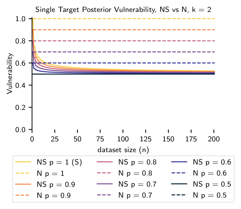
Figure 2: Posterior single-target vulnerability for binary attributes under a uniform prior over various dataset sizes $n$. We consider the $k$-RR channel N, the composition of $k$-RR & shuffle NS, and the shuffle channel S (when $p=1$).

Fig. 2 compares posterior single-target vulnerability for binary attributes under the shuffling channel S, under the $k$-RR mechanism N, and under the $k$-RR and shuffle cascade NS, for various values of the $k$-RR parameter $p$.

Notice that the dotted yellow line represents a baseline of no security measures: when only $k$-RR N is applied using parameter $p=1$, every participant reports their true value, and no shuffle is applied. This line represents an upper bound on the posterior vulnerability, since in the absence of any protective measure the adversary will know a target’s value with certainty, and so the vulnerability is 1. However, when a shuffle is performed, as represented by the solid yellow line, the vulnerability drops immediately and dramatically, even if no noise is added. More precisely, since $p=1$, this line represents exactly the vulnerability $V_{g_{\rm T}}[\pi\triangleright\textnormal{{S}}]$.

The dotted lines represent the posterior vulnerability under a $k$-RR channel N for different values of $p$. We see that adding more noise improves the security of a single target’s value. As $p$ decreases, users are less likely to report their true values, thereby decreasing the adversary’s probability of guessing correctly. For example, if a user reports their true value with probability $p=0.9$, the adversary will only guess the correct value $\nicefrac{{9}}{{10}}$ of the time, represented by the dotted orange line. The vulnerability under $k$-RR is not affected by the dataset size, and thus remains constant for all $n$.

The remaining solid lines indicate the posterior vulnerability under the cascade NS. We see here that shuffling noisy data exponentially decreases the vulnerability. At $n=1$, the adversary observes only one value, and will know with certainty that it belongs to the target. When $p=0.9$, she will guess the reported value and be correct $90\%$ of the time. But when $n=2$, she could observe any of the following histograms: $\texttt{a}{:}2,\texttt{b}{:}0$, or $\texttt{a}{:}1,\texttt{b}{:}1$, or $\texttt{a}{:}0,\texttt{b}{:}2$. If she observes $\texttt{a}{:}2,\texttt{b}{:}0$, she will guess aand be correct $\nicefrac{{9}}{{10}}$ of the time; likewise if she observes $\texttt{a}{:}0,\texttt{b}{:}2$, she will guess b. However, if she observes $\texttt{a}{:}1,\texttt{b}{:}1$ (which she will observe $\nicefrac{{1}}{{2}}$ the time), either guess has an equal probability of being correct, decreasing the total vulnerability from $\nicefrac{{9}}{{10}}$ to $\nicefrac{{7}}{{10}}$. As $n$ grows, there are more possible outputs where the division of $n$ is less clear, bring the vulnerability closer to $\nicefrac{{1}}{{2}}$. At $n=200$, the posterior vulnerability of NS $p=0.9$ is $0.5225$.

Note that the solid lines representing NS do not coincide at $n=200$, although they will converge as $n$ grows. Concretely, given cascade NS at $n=200$, the vulnerability when $p=1$ is approximately $0.5282$ and the vulnerability when $p=0.6$ is approximately $0.5056$.

This graph shows that, for many values of $p$, shuffling alone is more effective in reducing vulnerability than simply adding noise. At $n=200$, the posterior vulnerability of a shuffle with no noise represented by the solid yellow line is approximately $0.5286$, which means a shuffle alone has lower vulnerability than an application of noise where $p\geq 0.53$. This happens for most values of $p$. The only choice of $p$ that improves upon the security of a shuffle alone is when $p$ approaches $\nicefrac{{1}}{{2}}$.

V Single-target leakage of a binary value against a strong adversary

Thus far, our analysis has centered on specific adversary with limited prior knowledge , since they can often benefit the most from inference attacks. However, since differential privacy guarantees are crafted for the strong adversary, who a priori knows everyone’s data but one, in this section we introduce a preliminary discussion about how vulnerability changes under this strong, all-but-one (ABO), adversary.

Returning to Example 6, consider a dataset $n=3$ and assume the adversary knows a priori that the last two people have a’s. The set of secrets is reduced from $2^{8}$ to 2: aaa or baa. How does observing the channel output affect the adversary’s ability to guess the target’s value?

Under shuffling alone, the adversary could observe histogram $\texttt{a}:2,~{}\texttt{b}:1$ and know with certainty that $x_{0}=\texttt{b}$, or she could observe $\texttt{a}:3$ and know with certainty that $x_{0}=\texttt{a}$; the posterior ABO vulnerability is therefore 1. Under the $k$-RR channel, she will guess what she sees and she can be confident about this guess with probability $p$. Through QIF, we can illustrate how vulnerability can decrease when the two mechanisms are combined in NS.

From [14], posterior vulnerability can be calculated by summing column maximums and scaling by the prior probability.

$$V_{ABO}[\pi\triangleright\textnormal{{NS}}^{r}]=\frac{1}{2}\sum_{y}\max_{\begin{subarray}{c}x_{0}=\texttt{a},\\ x_{0}=\texttt{b}\end{subarray}}\textnormal{{NS}}^{r}_{x,y}$$ (10)

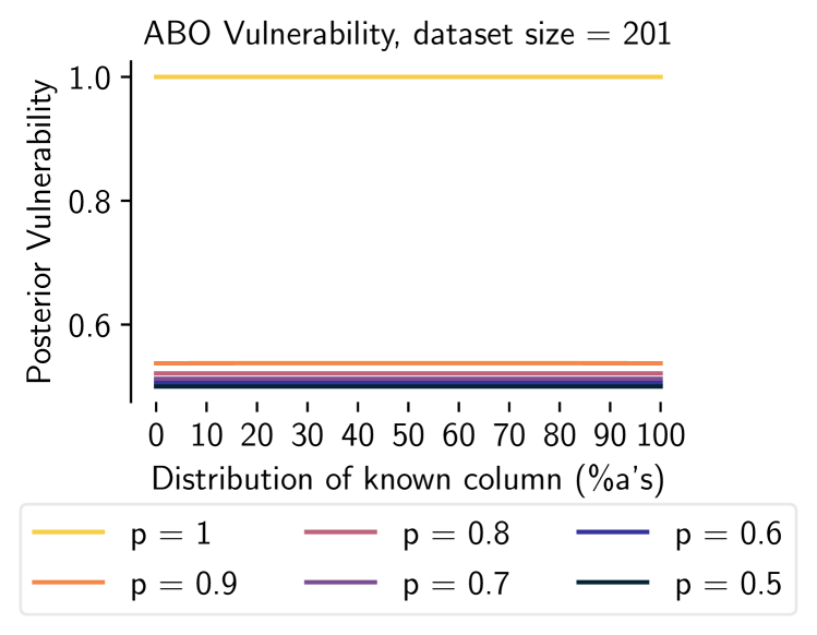
Figure 3: All-But-One posterior vulnerability when the dataset size $n=201$ and the adversary knows 200 values a priori.

Figure 3 shows the posterior ABO vulnerability when $n=201$, over different sets of adversary prior knowledge. The first $0\%$ tick represents an adversary who knows the last two hundred people have b’s, and who is guessing the value of the first person. Given this knowledge, when $p=0.8$, the ABO vulnerability is approx. 0.52111. Changing the prior distribution affects the ABO vulnerability, but only marginally. For instance, when the adversary knows that one hundred people have a’s and the other hundred have b’s (represented by the $50\%$ tick), the vulnerability increases a bit, but only to approx. 0.52116.

From the graph, we can confirm that the shuffle alone (represented by the yellow line when $p=1$) does not affect vulnerability—the adversary can guess the last person with perfect confidence. Recall that the opposite effect was observed in Figure 2 where the shuffle alone dramatically reduced vulnerability; this speaks to how adversary choice influences our understanding of a given privacy mechanism. However, when noise is introduced, the vulnerability decreases below $p$, indicating that the combination of noise and shuffling provides the most security. A formal investigation of this phenomena is set for future work.

VI Single-target leakage of a generic value $k{\geq}2$ against an uninformed adversary

In this section, we extend our investigation of Sec. IV to attack scenarios in which: (i) as before, the adversary is attempting to guess the secret value of a single individual from $\mathcal{N}$ chosen as the target in the dataset; but (ii) contrarily to before, the set $\mathcal{K}$ of sensitive values can have any size $k{\geq}2$. Here again, we focus on an uninformed adversary, with a uniform prior on datasets.

For this general case, we develop exact equations with which to calculate single-target posterior vulnerability. However, these equations are not as computationally efficient or as easy to analyze as the binary case. Nevertheless, we are able to provide asymptotic bounds on leakage by uncovering a surprising connection between our scenario and a well-known combinatorial problem.

VI-A Leakage formulas

The prior vulnerability remains $\nicefrac{{1}}{{k}}$, the same as that of the binary case, per Prop. 14. Indeed, given a uniform distribution, an adversary will guess any of the $k$ values and will have an equal probability of being correct.

For posterior vulnerability, we investigate the same combinations of sanitization mechanisms as before: the $k$-RR channel N, the full shuffle channel S, and the composition of $k$-RR with shuffle via the cascade NS. The posterior vulnerability of the $k$-RR channel N has already been derived in Prop. 15 for any $k\geq 2$, and it is simply $p$. However, the vulnerability of the shuffle channel S and consequently of the cascade NS depends on $k$, necessitating a generalization of the earlier results.

Recall that under shuffling, the exact mapping from individuals to values is lost, and only the dataset’s histogram is preserved. In the binary case, the posterior vulnerability of shuffling was computed by iterating through all histograms of size two, which could be counted using a summation of binomial coefficients. In the general case, the adversary observes multi-sets, which must be counted using multinomial coefficients, as formalized below.

Proposition 20 (Posterior single-target vulnerability under shuffle and $k\geq 2$).

Given the same hypotheses as Prop. 16, except that the sensitive set $\mathcal{K}$ can have $k\geq 2$ elements,

$$V_{g_{\rm T}}[\pi\triangleright\textnormal{{S}}]=V_{g_{\rm T}}[\pi\triangleright\textnormal{{S}}^{r}]=\frac{1}{k^{n}}\sum_{\begin{subarray}{c}n_{1},\dots,n_{k}:\\ n_{1}+\dots+n_{k}=n\end{subarray}}\binom{n}{n_{1},\dots,n_{k}}\frac{n^{*}}{n},$$ (11)

where $n^{*}=\max(n_{1},\dots,n_{k})$.

Finally, the vulnerability of the combination of $k$-RR and shuffle is an extension of the binary case from Prop. 19.

Proposition 21 (Posterior single-target vulnerability under $k$-RR & shuffle, $k\geq 2$).

Given the same hypotheses as Prop. 18, except that the sensitive set $\mathcal{K}$ can have $k\geq 2$ elements,

$$V_{g_{\rm T}}[\pi\triangleright\textnormal{{NS}}]=V_{g_{\rm T}}[\pi\triangleright\textnormal{{NS}}^{r}]=$$

$$\frac{1}{k^{n}}\sum_{\begin{subarray}{c}n_{1},\dots,n_{k}:\\ n_{1}+\dots+n_{k}=n\end{subarray}}\binom{n}{n_{1},\dots,n_{k}}\frac{n^{*}p+(n{-}n^{*})\nicefrac{{(1{-}p)}}{{(k{-}1)}}}{n}$$ (12)

where $n^{*}=\max(n_{1},\dots,n_{k})$.

Notice, however, that the formulas given in Prop. 20 and Prop. 21, although exact, are not easy to compute or interpret. Indeed, they depend on the computation of a number of binomial coefficients that grows linearly with the dataset size $n$. In Sec. VI-C, we shall discuss asymptotic bounds for these vulnerabilities, but first we analyze the exact behavior of leakage for tractable values of $n$, $k$, and $p$.

VI-B Analyses of leakage behavior

Fig. 4 compares the exact values for the posterior vulnerabilities of the three channels N, S, and NS for a set $\mathcal{K}$ of sensitive values with $k=5$ elements.

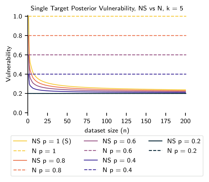
Figure 4: Posterior single-target vulnerability for $k=5$ values, under a uniform prior over various dataset sizes $n$. We consider the $k$-RR channel N, the composition of $k$-RR & shuffle NS, and the shuffle channel S ($p=1$).

As before, the dotted yellow line represents the case of no noise nor shuffle; here, the adversary can observe and know the target’s value exactly. By observing the vulnerability under the shuffle channel S, represented by the solid yellow line, we can see that shuffle alone decreases the adversary’s probability of success considerably. The dotted lines represent the vulnerability under the $k$-RR channel N for different values of $p$, while the solid lines represent posterior vulnerability under the NS cascade. For example, when $p=0.8$, represented by the dotted orange line, the posterior vulnerability drops to $0.8$, regardless of the dataset size. When shuffle is added, the vulnerability drops exponentially with $n$, represented by the solid orange line, asymptotically approaching the lower bound of $0.2=\nicefrac{{1}}{{k}}$ (the prior vulnerability). The graph suggests that shuffle alone is a highly effective sanitization mechanism, significantly outperforming $k$-RR’s leakage guarantees in most cases. Indeed, the only cases in which $k$-RR alone provides a sanitization comparable to that provided by shuffle alone are when the parameter $p$ approaches $\nicefrac{{1}}{{k}}$. However, these are exactly the cases in which the mechanisms are noisiest, so their utility suffers the most.

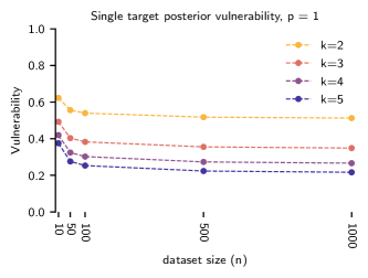
Figure 5: Posterior single-target vulnerability of the shuffle channel S under a uniform prior, for varying attribute set sizes $k$ and dataset sizes $n$.

Fig. 5 provides more insight into how shuffle alone affects posterior vulnerability. As exact values are computationally expensive to calculate as $n$ and $k$ increase, here we show the exact vulnerability for a subset of dataset sizes $n$ ranging from 10 to 1000. We see that posterior vulnerability decreases with $n$, and approaches the prior vulnerability of $\nicefrac{{1}}{{k}}$. For the sake of comparison, at $n=100$ the posterior vulnerability when $k=3$ is $0.3826$, and at $n=1000$ it is $0.3488$.

VI-C Asymptotic Bounds

Interestingly, (11) has an important combinatorial interpretation when scaled up by $n$, which can be written explicitly as

$$V_{g_{\rm T}}[\pi\triangleright\textnormal{{S}}]\times n=\frac{1}{k^{n}}\sum_{\begin{subarray}{c}n_{1},n_{2},\dots,n_{k}:\\ n_{1}+n_{2}+\dots+n_{k}=n\end{subarray}}\binom{n}{n_{1},n_{2},\dots,n_{k}}n^{*}.$$ (13)

Intuitively, when $n$ balls are thrown uniformly at random and independently into $k$ distinct bins, (13) computes the exact number of expected balls in the fullest bin (also referred to as “maximum load”). This perspective provides an interpretation of (11): For every division of $n$ into $k$ parts, this equation counts the ways these parts can be labeled, chooses the largest part, then takes the average by dividing by the total number of the possibilities. Brown’s work on surmising remixed keys [52] posits an equivalent formula for Equ. 13, however he too was unable to find a faster way to compute these values exactly. This connection is discussed in Appendix -B.

There are well-known asymptotic bounds for this combinatorial problem [53]. In particular, when $n\geq k\ln k$,

$$V_{g_{\rm T}}[\pi\triangleright\textnormal{{S}}]\times n=\frac{n}{k}+\Theta\left(\sqrt{\frac{n\ln k}{k}}\right)\quad\textnormal{(maximum load)}$$ (14)

This holds with high probability, meaning an event $M$ counting the maximum number of $n$ balls in $k$ bins occurs with probability Pr$(M)\geq 1-k^{-c}$ for an arbitrarily chosen constant $c\geq 0$ [54]. Dividing both sides by $n$, we get asymptotic bounds for posterior single-target vulnerability.

$$V_{g_{\rm T}}[\pi\triangleright\textnormal{{S}}]=\frac{1}{k}+\Theta\left(\sqrt{\frac{\ln k}{kn}}\right)$$ (15)

These bounds show the maximum load grows sublinearly with $n$ while posterior vulnerability decreases monotonically.

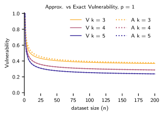
Figure 6: Comparison of the approximation with the true value of posterior single-target vulnerability through the shuffle channel for different values of $k$.

While the big-theta implies the existence of a constant factor $f$, we can test how well this equation matches the true posterior vulnerability when $f=1$. Fig. 6 shows how well the asymptotic bounds for posterior single-target vulnerability under the shuffle channel approximate the exact value. The yellow line, representing the exact vulnerability when $k=3$, has a slight offset from the approximation, but the violet and blue lines, representing $k=4$ and $k=5$ respectively, are visually indistinguishable from the value provided by the asymptotic bounds.

Given an approximation for $V_{g_{\rm T}}[\pi\triangleright\textnormal{{S}}]$, we can derive an approximation for $V_{g_{\rm T}}[\pi\triangleright\textnormal{{NS}}]$.

Theorem 22.

Posterior single-target vulnerability for a general $k$ has the following asymptotic bounds.

$$V_{g_{\rm T}}[\pi\triangleright\textnormal{{NS}}]=\frac{1}{k}+\Theta\left(\sqrt{\frac{\ln k}{kn}}\right)\left(\frac{kp-1}{k-1}\right)$$ (16)

The proof relies on the fact that the equation for posterior vulnerability under NS can be re-written as a function of the posterior vulnerability under S. Explicitly,

$$V_{g_{\rm T}}[\pi\triangleright\textnormal{{NS}}]=V_{g_{\rm T}}[\pi\triangleright\textnormal{{S}}]\times\left(\frac{kp-1}{k-1}\right)+\frac{1-p}{k-1}.$$ (17)

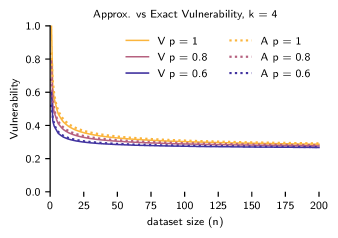
Figure 7: Comparison of the approximation with the true value of posterior single-target vulnerability through the shuffle and $k$-RR channels when $k=4$ for different values of $p$.

Fig. 7 sets $k=4$ and compares the exact posterior single-target vulnerability with the asymptotic bounds assuming $f=1$. When $p=1$, we see the dotted yellow line representing the bounds is slightly above the straight yellow line representing the exact value for small values of $n$. As $n$ increases, the two lines converge. This is seen again for $p=0.8$ and $p=0.6$. From this anecdotal test, it seems the asymptotic bound closely approximates the true value when $f=1$.

VII Discussion

The main lessons learned from this work are the following:

• The shuffle and the $k$-RR mechanisms commute, in the sense that their composition as probabilistic functions commute. We believe that this is the case for the composition of the shuffle with any local obfuscation mechanism.

• By using the formulas derived for vulnerabilities and leakage, we have shown that under the uninformed adversary the shuffling accounts for most of the privacy, as by itself it achieves almost the same level of resilience to inference attatcks as its composition with $k$-RR. (The only exception is when the probability of reporting the true value is $p=\nicefrac{{1}}{{k}}$, but this case has no utility.) We also noted that the level of posterior vulnerability decreases very fast with the number of participants, and that it converges to the prior, which is $\nicefrac{{1}}{{k}}$, i.e., the probability of guessing the true value by making a random guess.

• We have shown how to model the strong adversary in our framework, and how to calculate the posterior vulnerability. Our experiments show that, under the strong adversary, shuffling alone is ineffective, but it substantially increases privacy when combined with $k$-RR. This reinforces the results from the shuffle model literature pointing out the merits of shuffling, like for example [27], although in general those works consider adversaries even more powerful than the strong adversary of DP.

• As a consequence of the above findings, we point out that, for achieving the best trade-off between privacy and utility, in the strong model it is better to compose $k$-RR and shuffle. In contrast, under the uninformed adversary, it may be better to use the shuffle alone, as $k$-RR reduces utility and does not have a significant impact on privacy.

• Our results can help to choose, among two or more mechanisms (for instance, the shuffle model alone or the shuffle combined with $k$-RR), the one that gives the best trade-off between privacy and utility. Indeed, by using the formulas derived for the posterior vulnerability, we can compute the level of privacy (i.e., resilience to inference attacks) of the mechanisms and compare them. This process may also require to tune $\epsilon$ so to achieve the desired utility. We remark that different adversary models may lead to different results in this comparison, as shown in the introduction. We argue that, in case we don’t know what kind of adversary we will have to face, it is generally better to choose the more likely one. In the case of DP, a basic assumption is that the data consumer cannot access directly the database, it can only query it, via the interface (the database curator). Hence the uninformed adversary is more natural and likely than the strong one.

VIII Conclusion

In this work, we proved that $k$-RR and shuffling can commute without affecting information leakage, and derived exact formulas for prior and posterior vulnerabilities for an uninformed adversary focusing on a single target. For binary attributes, these formulas are computationally efficient, and for the general case we found asymptotic bounds. We studied how the leakage of shuffling and $k$-RR mechanisms behaves as the dataset size increases for different privacy parameters. For the uninformed adversary, we found that shuffling alone may dramatically reduce leakage in many cases, outperforming the application of $k$-RR alone.

-A Reduced $k$-RR mechanism and its compositional properties

Here we complement the discussion on reduced mechanisms, presented in Sec. III-B, by introduced a reduced version of the $k$-RR mechanism and proving its compositional properties with the reduced shuffling mechanism.

Reduced channel for the $k$-RR mechanism

For completeness, we can also consider a reduced version of the $k$-RR mechanism that operates by taking a histogram as input and producing a histogram over randomized values as output.

We want to define the reduced channel $k$-RR operating directly over histograms so that its final effect is the same as the expected effect of a full $k$-RR channel operating over all concrete datasets with the same histogram as the input histogram, weighted by uniform prior distribution on datasets.

Formally, let $Pr(x,y,z_{1},z_{2})$ denote the joint probability over datasets $x,y\in\mathcal{K}^{n}$ and histograms $z_{1},z_{2}$ over $\mathcal{K}$. We will derive the reduced $k$-RR channel $\textnormal{{N}}^{r}$ mapping histograms to histograms by imposing restrictions on this joint probability. We start by deriving, for all histograms $z_{1},z_{2}$ over $\mathcal{K}$:

$$\textnormal{{N}}^{r}_{z_{1},z_{2}}=\text{(def.\ of channel)}$$

$$Pr(z_{2}\mid z_{1})=\text{(marginalization)}$$

$$\textstyle\sum_{\begin{subarray}{c}x\in\mathcal{K}^{n}\\ y\in\mathcal{K}^{n}\end{subarray}}\,\,Pr(x,y,z_{2}\mid z_{1})=\text{(chain rule)}$$

$$\textstyle\sum_{\begin{subarray}{c}x\in\mathcal{K}^{n}\\ y\in\mathcal{K}^{n}\end{subarray}}\,\,Pr(x\mid z_{1})Pr(y\mid x,z_{1})Pr(z_{2}\mid x,y,z_{1})$$ (18)

Now, we impose the restriction that $Pr(y\mid x,z_{1})$ must be exactly the probability $\textnormal{{N}}_{x,y}$ that the corresponding full channel N operating on a dataset $x$ would produce dataset $y$ as output. We also impose that $z_{2}$ must be the histogram of dataset $y$, so $Pr(z_{2}\mid x,y,z_{1})$ must be 1 exactly when $h(y)=z_{2}$, and 0 otherwise. By applying that to (-A), we get:

$$\textnormal{{N}}^{r}_{z_{1},z_{2}}= \,\,\textstyle\sum_{\begin{subarray}{c}x\in\mathcal{K}^{n}\\ y\in\mathcal{K}^{n}:h(y)=z_{2}\end{subarray}}Pr(x\mid z_{1})\textnormal{{N}}_{x,y}$$ (19)

Now let us denote by $\pi_{x\mid z_{1}}$ the conditional probability $Pr(x\mid z_{1})$ that the input dataset is $x$ given that its histogram must be $z_{1}$. Considering that the distribution on input datasets is uniform, as per (5), we then derive:

$$\pi_{x\mid z_{1}}=Pr(x\mid z_{1})=\begin{cases}\nicefrac{{1}}{{\#h(x)}},&\text{if $h(x)=z_{1}$},\\ 0,&\text{otherwise}.\end{cases}$$ (20)

Finally, by substituting (20) in (19), we reach the definition of a reduced shuffling channel $\textnormal{{N}}^{r}$ below.

Definition 23 (Reduced $k$-RR channel).

Given a uniform prior $\pi$ on all possible original datasets $x\in\mathcal{K}^{n}$, a reduced $k$-RR channel $\textnormal{{N}}^{r}$ (again, for “noise”) is a channel from histograms on $\mathcal{K}$ to histograms on $\mathcal{K}$ s.t., for every input histogram $z_{1}$ and output histogram $z_{2}$,

$$\textnormal{{N}}^{r}_{z_{1},z_{2}}=\textstyle\sum_{\begin{subarray}{c}x\in\mathcal{K}^{n}:h(x)=z_{1}\\ y\in\mathcal{K}^{n}:h(y)=z_{2}\end{subarray}}\frac{1}{\#h(x)}\textnormal{{N}}_{x,y}.$$

Example 24 (Reduced $k$-RR channel).

Table IV contains the channel $\textnormal{{N}}^{r}$ representing the application of a reduced $k$-RR mechanism to the scenario of Example 6.

$\textnormal{{N}}^{r}$	a:3, b:0	a:2, b:1	a:1, b:2	a:0, b:3
a:3, b:0	$p^{3}$	$3p^{2}\overline{p}$	$3p\overline{p}^{2}$	$\overline{p}^{3}$
a:2, b:1	$p^{2}\overline{p}$	$\nicefrac{{(p^{3}+2p\overline{p}^{2})}}{{3}}$	$\nicefrac{{(2p^{2}\overline{p}+\overline{p}^{3})}}{{3}}$	$p\overline{p}^{2}$
a:1, b:2	$p\overline{p}^{2}$	$\nicefrac{{(2p^{2}\overline{p}+\overline{p}^{3})}}{{3}}$	$\nicefrac{{(p^{3}+2p\overline{p}^{2})}}{{3}}$	$p^{2}\overline{p}$
a:0, b:3	$\overline{p}^{3}$	$3p\overline{p}^{2}$	$3p^{2}\overline{p}$	$p^{3}$

TABLE IV: Reduced $k$-RR channel $\textnormal{{N}}^{r}$ for Example 24, with $k{=}2$ possible sensitive values and $n{=}3$ individuals. The channel receives histograms as inputs and produces histograms as outputs.

In contrast to the case regarding shuffling channels, the full $k$-RR channel N and its reduced counterpart $\textnormal{{N}}^{r}$ are not equivalent. Indeed, they are not even comparable w.r.t, since they do not have the same input type.

Proposition 25 (Non-equivalence between full and reduced $k$-RR).

Let N be a full $k$-RR channel as per Def. 10, and $\textnormal{{N}}^{r}$ be the reduced $k$-RR channel obtained from N as per Def. 23. Then

$$\textnormal{{N}}\not\equiv\textnormal{{N}}^{r}.$$

Compositions of reduced mechanisms

As with their full counterparts ( mapping datasets to datasets), the reduced sanitization mechanisms ( operating over histograms) can be applied to an input dataset either in isolation or in combination.

The situation regarding reduced mechanisms, however, is more subtle. Notice that we are allowed to cascade a reduced shuffling channel $\textnormal{{S}}^{r}$ with a reduced $k$-RR channel $\textnormal{{N}}^{r}$, since the output of the former and the input of the latter are both histograms, and the first channel operates on datasets. But we cannot start our sanitization process by applying a reduced $k$-RR channel $\textnormal{{N}}^{r}$ to a dataset, since this channel receives as input only histograms. It turns out, however, that a meaningful form of commutativity between shuffling and $k$-RR holds if we are careful with the types of the channels in the cascade, as depicted in Fig. 8. That is formalized in the following result.

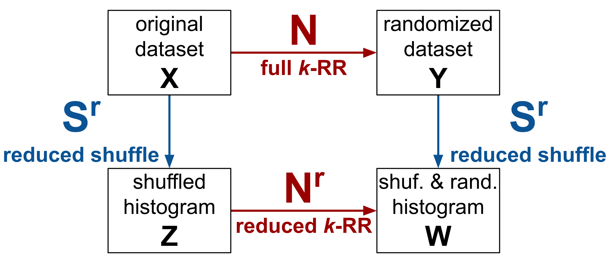
Figure 8: Commutativity in the reduced case: $\textnormal{{N}}\textnormal{{S}}^{r}=\textnormal{{S}}^{r}\textnormal{{N}}^{r}$. Channel N maps datasets to datasets, channel $\textnormal{{S}}^{r}$ maps datasets to histograms, and channel $\textnormal{{N}}^{r}$ maps histograms to histograms.

Proposition 26 (Commutativity of $k$-RR and shuffling: Reduced case).

Let $\mathcal{N}=\{0,1,\ldots,n-1\}$ be a set of $n\geq 1$ individuals and $\mathcal{K}$ be a set of $k\geq 2$ values for the sensitive attribute. Let also N be a full $k$-RR channel as per Definition 10, $\textnormal{{N}}^{r}$ be a reduced $k$-RR channel as per Definition 23, and $\textnormal{{S}}^{r}$ be a reduced shuffling channel per Definition 8. Then

$$\textnormal{{N}}\textnormal{{S}}^{r}=\textnormal{{S}}^{r}\textnormal{{N}}^{r}.$$

Example 27 (Cascading of $k$-RR and shuffling in the reduced case).

Consider again the scenario of Example 6. The channel $\textnormal{{N}}\textnormal{{S}}^{r}$ representing the application of a full $k$-RR mechanism followed by reduced shuffling and the channel $\textnormal{{S}}^{r}\textnormal{{N}}^{r}$ representing the application of reduced shuffling followed by a reduced $k$-RR mechanism are identical, as represented in Table V.

$\textnormal{{N}}\textnormal{{S}}^{r}$/$\textnormal{{S}}^{r}\textnormal{{N}}^{r}$	(a:3,b:0)	(a:2,b:1)	(a:1,b:2)	(a:0,b:3)
aaa	NSrc1$p^{3}$	NSrc2$3p^{2}\overline{p}$	NSrc3$3p\overline{p}^{2}$	NSrc4$\overline{p}^{3}$
aab	NSrc5$p^{2}\overline{p}$	NSrc6$p^{3}+2p\overline{p}^{2}$	NSrc7$2p^{2}\overline{p}+\overline{p}^{3}$	NSrc8$p\overline{p}^{2}$
aba	NSrc5$p^{2}\overline{p}$	NSrc6$p^{3}+2p\overline{p}^{2}$	NSrc7$2p^{2}\overline{p}+\overline{p}^{3}$	NSrc8$p\overline{p}^{2}$
baa	NSrc5$p^{2}\overline{p}$	NSrc6$p^{3}+2p\overline{p}^{2}$	NSrc7$2p^{2}\overline{p}+\overline{p}^{3}$	NSrc8$p\overline{p}^{2}$
abb	NSrc8$p\overline{p}^{2}$	NSrc7$2p^{2}\overline{p}+\overline{p}^{3}$	NSrc6$p^{3}+2p\overline{p}^{2}$	NSrc5$p^{2}\overline{p}$
bab	NSrc8$p\overline{p}^{2}$	NSrc7$2p^{2}\overline{p}+\overline{p}^{3}$	NSrc6$p^{3}+2p\overline{p}^{2}$	NSrc5$p^{2}\overline{p}$
bba	NSrc8$p\overline{p}^{2}$	NSrc7$2p^{2}\overline{p}+\overline{p}^{3}$	NSrc6$p^{3}+2p\overline{p}^{2}$	NSrc5$p^{2}\overline{p}$
bbb	NSrc4$\overline{p}^{3}$	NSrc3$3p\overline{p}^{2}$	NSrc2$3p^{2}\overline{p}$	NSrc1$p^{3}$

TABLE V: Channel for Example 27, representing both the cascading $\textnormal{{N}}\textnormal{{S}}^{r}$ of full $k$-RR followed by reduced shuffling and the cascading $\textnormal{{S}}^{r}\textnormal{{N}}^{r}$ of reduced shuffling followed by reduced $k$-RR, with $k{=}2$ possible sensitive values and $n{=}3$ individuals. Here $p$ is the probability a user responds with their true value, and $\overline{p}{=}1{-}p$. The cells are colored according to the entries’ values when $p{=}0.75$ and $\overline{p}{=}0.25$. Here $p^{3}+2p\overline{p}^{2}$ represents the largest value at approximately 0.5156 while $\overline{p}^{3}$ is the smallest at approximately 0.0156.

Finally, we provide the following result, stating that the composed mechanisms of shuffling and $k$-RR in their full and reduced forms are equivalent, in the sense that, for every $g$-vulnerability measure and prior distribution on secret values, both yield the same quantification of information leakage.

Proposition 28 (Equivalence of full and reduced compositions).

Let $\mathcal{N}=\{0,1,\ldots,n-1\}$ be a set of $n\geq 1$ individuals and $\mathcal{K}$ be a set of $k\geq 2$ values for the sensitive attribute. Let also N be a full $k$-RR channel as per Definition 10, $\textnormal{{N}}^{r}$ be a reduced $k$-RR channel as per Definition 23, and $\textnormal{{S}}^{r}$ be a reduced shuffling channel per Definition 8. Then:

$$\textnormal{{S}}\textnormal{{N}}\equiv \,\,\textnormal{{S}}^{r}\textnormal{{N}}^{r}$$ (21)

Fig. 9 extends Fig. 1 and summarizes all relationships among compositions of the full and reduced versions of both the $k$-RR mechanism and of shuffling.

$\begin{array}[]{rcl}&\text{\small Prop.~{}\ref{prop:equivalence-S}}&\\ \textnormal{{S}}&\text{\LARGE$\equiv$}&\textnormal{{S}}^{r}\\ \end{array}$    $\begin{array}[]{rcl}&\text{\small Prop.~{}\ref{prop:nonequivalence-N}}&\\ \textnormal{{N}}&\text{\LARGE$\not\equiv$}&\textnormal{{N}}^{r}\\ \end{array}$
$\begin{array}[]{rcl}&\text{\small Prop.~{}\ref{theorem:equivalenceCompositions-A}}&\\ \textnormal{{N}}\textnormal{{S}}&\text{\LARGE$\equiv$}&\textnormal{{N}}\textnormal{{S}}^{r}\\ \text{\small Prop.~{}\ref{theorem:commutativity-full}}\,\,\,\,\rotatebox[origin={c}]{90.0}{\LARGE$\equiv$}&&\,\,\,\,\rotatebox[origin={c}]{90.0}{\LARGE=}\,\,\,\,\text{\small Prop.~{}\ref{theorem:commutativity-reduced}}\\ \textnormal{{S}}\textnormal{{N}}&\text{\LARGE$\equiv$}&\textnormal{{S}}^{r}\textnormal{{N}}^{r}\\ &\text{\small Prop.~{}\ref{theorem:equivalenceCompositions-B}}&\\ \end{array}$

Figure 9: All relationships among compositions of full and reduced $k$-RR and shuffling, extending the results from Fig. 1. Here $(=)$ denotes syntactic equality, whereas $(\equiv)$ denotes equivalence w.r.t. information leakage.

-B Using Integer Partitions

Although Prop. 20 and Prop. 21 provide exact values for posterior vulnerability under the shuffle and $k$-RR channels, the formulas are computationally expensive.

We can improve these formulas by eliminating computational redundancies in (11). E.g., when $n{=}6$ and $k{=}3$, an adversary could observe a:2, b:3, c:1 (so $n_{1}{=}2$, $n_{2}{=}3$, $n_{3}{=}1$), or they could observe a:3, b:1, c:2 (so $n_{1}{=}3$, $n_{2}{=}1$, $n_{3}{=}2$). Both cases have the same multinomial coefficient and maximum $n^{*}$. Notice that the exact assignment of value to $n^{*}$ does not matter, as long as they are all accounted for. With this insight, we follow [55] and use integer partitions, i.e., partitions of $n$ into exactly $k$ parts such that their elements sum to $n$. E.g., when $n{=}6$ and $k{=}3$, all relevant integer partitions are $[6,0,0],[5,1,0],[4,2,0],[4,1,1],[3,3,0],[3,2,1]$, and $[2,2,2]$. Instead of iterating through 28 multi-sets, we only need to consider 7 cases. Hence, we can rewrite (11) as

$$V_{g_{\rm T}}[\pi\triangleright\textnormal{{S}}]=V_{g_{\rm T}}[\pi\triangleright\textnormal{{S}}^{r}]=\frac{1}{k^{n}}\sum_{\lambda_{n,k}}\binom{n}{\lambda}\binom{k}{\bar{\lambda}\quad k-\ell(\lambda)}\frac{\lambda^{*}}{n},$$ (22)

where $\lambda$ is the integer partition of $n$, $\bar{\lambda}$ is the multiplicity of each value in the partition, $l$ is the length of $\lambda$, and $\lambda^{*}{=}\max_{i}\lambda_{i}$ is the maximum value in $\lambda$. E.g., given $n{=}20$ and $k{=}4$, when $\lambda=(8,8,1,1,1,1)$, then $\ell{=}6$, and $\bar{\lambda}{=}(4,2)$. Note that both coefficients here are multinomials, as $\lambda$ and often $\bar{\lambda}$ represent sets of numbers, and they always sum to $n$ and $k$ respectively. We can simplify this equation further if we adjust (22) by removing the prior distribution of the secrets, and multiplying the summation by $n$, therefore rewriting it as

$$\textstyle\sum_{\lambda_{n,k}}\binom{n}{\lambda}\binom{k}{\bar{\lambda}\quad k-\ell(\lambda)}\lambda^{*}~{}.$$ (23)

It turns out that Brown has investigated this problem on surmising remixed keys [52], where he uses the formulation

$$B_{n,k}=\textstyle\sum_{|\lambda|=n}\lambda^{*}\frac{n!}{\lambda!\bar{\lambda}!}\ell!\binom{k}{\ell},$$ (24)

where $\lambda^{*}$ is the maximum value in the integer partition. It can be shown that our formulation and Brown’s are equivalent.

Proposition 29.

Equations 23 and  24 are equivalent.

Brown, however, states that he was unable to find a faster way to compute these values exactly.

-C Proofs

In this section we provide proofs absent from the main body of the paper.

-C1 Auxiliary technical results

Lemma 30 (Probability that full $k$-RR produces an output with a specific histogram for a given input: Binary case).

Let $\mathcal{N}=\{0,1,\ldots,n-1\}$ be a set of $n\geq 1$ distinct individuals of interest, $\mathcal{K}=\{\texttt{a},\texttt{b}\}$ be binary set (i.e., $k=2$) for each individual’s possible sensitive attribute, and N be a full $k$-RR channel as per Def. 10. Then, the probability that an input dataset $x\in\mathcal{K}^{n}$ is mapped through N to an output dataset with histogram $h(y)=\texttt{a}{:}n_{\texttt{a}}(y),\texttt{b}{:}n_{\texttt{b}}(y)$, for some $y\in\mathcal{K}^{n}$, is given by

$$\sum_{w\in\mathcal{K}^{n}:h(w)=h(y)}\textnormal{{N}}_{x,w}= \,\,\sum_{m_{\texttt{a}}=\max(n_{\texttt{a}}(x)-n_{\texttt{b}}(y),0)}^{\min(n_{\texttt{a}}(x),n_{\texttt{a}}(y))}\binom{n_{\texttt{a}}(x)}{m_{\texttt{a}}}\binom{n_{\texttt{b}}(x)}{n_{\texttt{b}}(x)-n_{\texttt{a}}(y)+m_{\texttt{a}}}p^{2m_{\texttt{a}}+n_{\texttt{b}}(x)-n_{\texttt{a}}(y)}\overline{p}^{n-2m_{\texttt{a}}-n_{\texttt{b}}(x)+n_{\texttt{a}}(y)}~{}.$$ (25)

Proof.

The proof can be constructed from the following observations:

1. From Def. 10, the mapping from an input dataset $x$ to an output dataset $w$ via the $k$-RR channel N can be seen as a Bernoulli process with $n$ independent tries (one for each individual in $x$), each having probability $p$ of $w_{i}$ matching the original value of $x_{i}$ (a “match”), and probability $\overline{p}=1-p$ of $w_{i}$ not matching the original value of $x_{i}$ (a “mismatch”).

2. Now, fix the dataset $x$, so all its elements, and, consequently, $n_{\texttt{a}}(x)$ and $n_{\texttt{b}}(x)$, are fixed. Fix also the histogram $h(w)$ of dataset $w$ to be the same histogram $h(y)$ of dataset $y$, so $n_{\texttt{a}}(w)=n_{\texttt{a}}(y)$ and $n_{\texttt{b}}(w)=n_{\texttt{b}}(y)$ are fixed, but not necessarily each entry $w_{i}=y_{i}$. Let $m(x,w)$ be the total number of matches in the mapping from a particular $x$ to a particular $w$ (i.e., the count of positions $i$ s.t. $x_{i}=w_{i}$). We can split $m$ into $m(x,w)=m_{\texttt{a}}(x,w)+m_{\texttt{b}}(x,w)$, where $m_{\texttt{a}}(x,w)$ and $m_{\texttt{b}}(x,w)$ are, respectively, the total number of matching a’s between $x$ and $w$ (i.e., the count of positions $i$ s.t. $x_{i}=w_{i}=\texttt{a}$) and the total number of matching b’s (i.e., the count of positions $i$ s.t. $x_{i}=w_{i}=\texttt{b}$).

3. The number $m_{\texttt{a}}(x,w)$ of matching a’s between $x$ and $w$ must respect the following inequalities.

   1. Its lower limit is

      $$m_{\texttt{a}}(x,w)\geq\max(n_{\texttt{a}}(x)-n_{\texttt{b}}(y),0)$$ (26)

      since for each mismatch of an a it is necessary to exist a b in $w$ paired up with an a in $x$. Hence, the number of mismatching a’s, given by $n_{\texttt{a}}(x)-m_{\texttt{a}}(x,w)$, can be at most the number $n_{\texttt{b}}(y)$ of b’s in $w$. This gives us $n_{\texttt{a}}(x)-m_{\texttt{a}}(x,w)\leq n_{\texttt{b}}(y)$, or, equivalently, $m_{\texttt{a}}(x,w)\geq n_{\texttt{a}}(x)-n_{\texttt{b}}(y)$. When $n_{\texttt{b}}(y)>n_{\texttt{a}}(x)$, this only tells us that $m_{\texttt{a}}(x,w)$ can be 0, since it can never be negative.

   2. Its upper limit is

      $$m_{\texttt{a}}(x,w)\leq\min(n_{\texttt{a}}(x),n_{\texttt{a}}(y)),$$ (27)

      since the number of matching a’s cannot be greater than the total number of a’s in $x$ or in $w$.

4. The number $m_{\texttt{b}}(x,w)$ of matching b’s is the following function of the numbers $n_{\texttt{a}}(x),n_{\texttt{b}}(x),n_{\texttt{a}}(y),n_{\texttt{b}}(y)$ of a’s and b’s in $x$ and $w$, and the number $m_{\texttt{a}}(x,w)$ of matching a’s between $x$ and $w$:

   $$m_{\texttt{b}}(x,w)=n_{\texttt{b}}(x)-n_{\texttt{a}}(y)+m_{\texttt{a}}(x,w),$$

   since once $m_{\texttt{a}}(x,w)$ values a are matched between $x$ and $w$, the other $n_{\texttt{a}}(x)-m_{\texttt{a}}(x,w)$ values a in $x$ must be paired up with that same number of b’s from $w$. So, from the total number $n_{\texttt{b}}(y)$ of b’s in $w$, only the remaining $n_{\texttt{b}}(y)-(n_{\texttt{a}}(x)-m_{\texttt{a}}(x,w))$ will produce a match with b’s from $x$. By substituting $n_{\texttt{b}}(y)=n-n_{\texttt{a}}(y)$ and $n_{\texttt{a}}(x)=n-n_{\texttt{b}}(x)$, we get to the equality above.

5. Now recall that we have already fixed $x$ (i.e., the value of each entry of $x_{i}$ of $x$ is fixed) and the histogram of $h(w)=h(y)$ (i.e., $n_{\texttt{a}}(w)=n_{\texttt{a}}(y)$ and $n_{\texttt{b}}(w)=n_{\texttt{b}}(y)$), but not necessarily the positions in which each a and b are in $w$. Let us go further and also fix the number $m_{\texttt{a}}(x,w)$ of matching a’s between $x$ and $w$ as well. From that, we have the following:

   1. To get exactly $m_{\texttt{a}}(x,w)$ matching a’s between $x$ and $w$, we need to pick from the $n_{\texttt{a}}(x)$ positions in $x$ with a’s the $m_{\texttt{a}}(x,w)$ ones which will be paired up with one of the $n_{\texttt{a}}(y)$ a’s from $w$. There are $\binom{n_{\texttt{a}}(x)}{m_{\texttt{a}}}$ ways of doing that.

   2. To get exactly $m_{\texttt{b}}(x,w)$ matching b’s between $x$ and $w$, we need to pick from the $n_{\texttt{b}}(x)$ positions in $x$ with b’s the $m_{\texttt{b}}(x,w)=n_{\texttt{b}}(x)-n_{\texttt{a}}(y)+m_{\texttt{a}}(x,w)$ ones which will be paired up with one of the $n_{\texttt{b}}(y)$ b’s from $w$. There are $\binom{n_{\texttt{b}}(x)}{n_{\texttt{b}}(x)-n_{\texttt{a}}(y)+m_{\texttt{a}}(x,w)}$ ways of doing that.

   3. The total number of matches between $x$ and $w$ is, then, $m_{\texttt{a}}(x,w)+m_{\texttt{b}}(x,w)=2m_{\texttt{a}}(x,w)+n_{\texttt{b}}(x)-n_{\texttt{a}}(y)$, and the total number of failures is $n-2m_{\texttt{a}}(x,w)-n_{\texttt{b}}(x)+n_{\texttt{a}}(y)$.

   Hence, the probability that N maps a fixed input dataset $x$ to an output dataset $w$ having histogram $h(y)$ and a fixed number $m_{\texttt{a}}(x,w)=m_{\texttt{a}}$ of matching a’s between input and output is

   $$\binom{n_{\texttt{a}}(x)}{m_{\texttt{a}}}\binom{n_{\texttt{b}}(x)}{n_{\texttt{b}}(x)-n_{\texttt{a}}(y)+m_{\texttt{a}}}p^{2m_{\texttt{a}}+n_{\texttt{b}}(x)-n_{\texttt{a}}(y)}\overline{p}^{n-2m_{a}-n_{\texttt{b}}(x)+n_{\texttt{a}}(y)}$$ (28)

6. Finally, we obtain the desired result in (25) by summing over all possible values $m_{\texttt{a}}$ of matching a’s given by (26) and (27).

∎

-C2 Proofs of Sec. III

See 9

Proof.

This follows from the fact that $\textnormal{{S}}^{r}$ is obtained from S only by the operation of merging columns that are multiples of each other, which does not alter vulnerability measures [14]. ∎

See 11

Proof.

For simplicity, we provide a proof for the case $\mathcal{K}$ has $k=2$ values; the case when $k\geq 2$ can be obtained as a direct generalization.

Notice that to achieve the desired result, it is sufficient to show the followin three points.

1. All columns of $(\textnormal{{N}}\textnormal{{S}})$ that represent output datasets with the same histogram are identical, i.e., for all datasets $x,y,y^{\prime}$ such that $h(y)=h(y^{\prime})$,

   $$(\textnormal{{N}}\textnormal{{S}})_{xy}=(\textnormal{{N}}\textnormal{{S}})_{xy^{\prime}}.$$ (29)

2. All columns of $(\textnormal{{S}}\textnormal{{N}})$ that represent output datasets with the same histogram are identical, i.e., for all datasets $x,y,y^{\prime}$ such that $h(y)=h(y^{\prime})$,

   $$(\textnormal{{S}}\textnormal{{N}})_{xy}=(\textnormal{{S}}\textnormal{{N}})_{xy^{\prime}}.$$ (30)

3. For every $x\in\mathcal{K}^{n}$ and histogram $z$ on $\mathcal{K}$,

   $$\sum_{\begin{subarray}{c}y\in\mathcal{K}^{n}:\\ h(y)=z\end{subarray}}(\textnormal{{N}}\textnormal{{S}})_{xy}=\sum_{\begin{subarray}{c}y\in\mathcal{K}^{n}:\\ h(y)=z\end{subarray}}(\textnormal{{S}}\textnormal{{N}})_{xy}.$$ (31)

Note that (29) and (30) tell us that in each channel the columns that represent the same histogram can be merged, since they are identical and that does not change leakage properties. Then, (31) tells us that the resulting channels are identical, since they both are defined as mappings from datasets to histograms, and all entries are identical.

To derive (29), notice that for all datasets $x,y,y^{\prime}$ s.t. $h(y)=h(y^{\prime})$:

$$(\textnormal{{N}}\textnormal{{S}})_{xy}= \,\,\sum_{w\in\mathcal{K}^{n}}\textnormal{{N}}_{x,w}\textnormal{{S}}_{w,y}$$ (matrix multiplication)

$$= \,\,\sum_{\begin{subarray}{c}w\in\mathcal{K}^{n}:\\ h(w)=h(y)\end{subarray}}\frac{1}{\#h(y)}\textnormal{{N}}_{x,w}$$ (Definition of S)

$$= \,\,\sum_{\begin{subarray}{c}w\in\mathcal{K}^{n}:\\ h(w)=h(y^{\prime})\end{subarray}}\frac{1}{\#h(y^{\prime})}\textnormal{{N}}_{x,w} h(y)=h(y^{\prime})$$ ()

$$= \,\,\sum_{w\in\mathcal{K}^{n}}\textnormal{{N}}_{x,w}\textnormal{{S}}_{w,y^{\prime}}$$ (matrix multiplication)

$$= \,\,(\textnormal{{N}}\textnormal{{S}})_{xy^{\prime}}$$

To derive (30), notice that for all datasets $x,y,y^{\prime}$ s.t. $h(y)=h(y^{\prime})$:

$$(\textnormal{{S}}\textnormal{{N}})_{xy}= \,\,\sum_{w\in\mathcal{K}^{n}}\textnormal{{S}}_{x,w}\textnormal{{N}}_{w,y}$$ (matrix multiplication)

$$= \,\,\sum_{\begin{subarray}{c}w\in\mathcal{K}^{n}:\\ h(w)=h(x)\end{subarray}}\frac{1}{\#h(x)}\textnormal{{N}}_{w,y}$$ (Definition of S)

$$= \,\,\frac{1}{\#h(x)}\sum_{\begin{subarray}{c}w\in\mathcal{K}^{n}:\\ h(w)=h(x)\end{subarray}}\textnormal{{N}}_{w,y}$$ (rearranging)

$$= \,\,\frac{1}{\#h(x)}\sum_{\begin{subarray}{c}w\in\mathcal{K}^{n}:\\ h(w)=h(x)\end{subarray}}\textnormal{{N}}_{y,w} \textnormal{{N}}_{w,y}=\textnormal{{N}}_{y,w}$$ ()

$$= \,\,\frac{1}{\#h(x)}\sum_{\begin{subarray}{c}w\in\mathcal{K}^{n}:\\ h(w)=h(x)\end{subarray}}\textnormal{{N}}_{y^{\prime},w}$$ (see below) (32)

$$= \,\,\frac{1}{\#h(x)}\sum_{\begin{subarray}{c}w\in\mathcal{K}^{n}:\\ h(w)=h(x)\end{subarray}}\textnormal{{N}}_{w,y^{\prime}} \textnormal{{N}}_{y^{\prime},w}=\textnormal{{N}}_{w,y^{\prime}}$$ ()

$$= \,\,\sum_{\begin{subarray}{c}w\in\mathcal{K}^{n}:\\ h(w)=h(x)\end{subarray}}\frac{1}{\#h(x)}\textnormal{{N}}_{w,y^{\prime}}$$ (rearranging)

$$= \,\,\sum_{w\in\mathcal{K}^{n}}\textnormal{{S}}_{x,w}\textnormal{{N}}_{w,y^{\prime}}$$ (Definition of S)

$$= (\textnormal{{S}}\textnormal{{N}})_{xy^{\prime}}$$ (matrix multiplication)

Note that step (32) follows because, from the proof of Lemma 30, $\textstyle\sum_{\begin{subarray}{c}w\in\mathcal{K}^{n}:\\ h(w)=h(x)\end{subarray}}\textnormal{{N}}_{y,w}$ depends only on the histogram of $y$, and not on its exact contents, so we can replace $y$ with $y^{\prime}$ as they have the same histogram.

Finally, to derive (31) we can reason:

$$\sum_{\begin{subarray}{c}y\in\mathcal{K}^{n}:\\ h(y)=z\end{subarray}}(\textnormal{{N}}\textnormal{{S}})_{xy}$$

$$=$$ (matrix multiplication)

$$\sum_{\begin{subarray}{c}y\in\mathcal{K}^{n}:\\ h(y)=z\end{subarray}}\sum_{w\in\mathcal{K}^{n}}\textnormal{{N}}_{x,w}\textnormal{{S}}_{w,y}$$

$$=$$ (Definition of S)

$$\sum_{\begin{subarray}{c}y\in\mathcal{K}^{n}:\\ h(y)=z\end{subarray}}\sum_{\begin{subarray}{c}w\in\mathcal{K}^{n}:\\ h(w)=h(y)\end{subarray}}\frac{1}{\#h(y)}\textnormal{{N}}_{x,w}$$

$$=$$ (rearranging)

$$\sum_{\begin{subarray}{c}y\in\mathcal{K}^{n}:\\ h(y)=z\end{subarray}}\frac{1}{\#h(y)}\sum_{\begin{subarray}{c}w\in\mathcal{K}^{n}:\\ h(w)=h(y)\end{subarray}}\textnormal{{N}}_{x,w}$$

$$=$$ (Lemma 30)

$$\sum_{\begin{subarray}{c}y\in\mathcal{K}^{n}:\\ h(y)=z\end{subarray}}\frac{1}{\#h(y)}\sum_{m_{\texttt{a}}=\max(n_{\texttt{a}}(x)-n_{\texttt{b}}(y),0)}^{\min(n_{\texttt{a}}(x),n_{\texttt{a}}(y))}\binom{n_{\texttt{a}}(x)}{m_{\texttt{a}}}\binom{n_{\texttt{b}}(x)}{n_{\texttt{b}}(x)-n_{\texttt{a}}(y)+m_{\texttt{a}}}p^{2m_{\texttt{a}}+n_{\texttt{b}}(x)-n_{\texttt{a}}(y)}\overline{p}^{n-2m_{\texttt{a}}-n_{\texttt{b}}(x)+n_{\texttt{a}}(y)}$$

$$= h(y)=h(z)\rightarrow n_{\texttt{a}}(y)=n_{\texttt{a}}(z) n_{\texttt{b}}(y)=n_{\texttt{b}}(z)$$ ( and )

$$\sum_{\begin{subarray}{c}y\in\mathcal{K}^{n}:\\ h(y)=z\end{subarray}}\frac{1}{\#h(y)}\sum_{m_{\texttt{a}}=\max(n_{\texttt{a}}(x)-n_{\texttt{b}}(z),0)}^{\min(n_{\texttt{a}}(x),n_{\texttt{a}}(z))}\binom{n_{\texttt{a}}(x)}{m_{\texttt{a}}}\binom{n_{\texttt{b}}(x)}{n_{\texttt{b}}(x)-n_{\texttt{a}}(z)+m_{\texttt{a}}}p^{2m_{\texttt{a}}+n_{\texttt{b}}(x)-n_{\texttt{a}}(z)}\overline{p}^{n-2m_{\texttt{a}}-n_{\texttt{b}}(x)+n_{\texttt{a}}(z)}$$

$$=$$ (rearranging the summation)

$$\sum_{m_{\texttt{a}}=\max(n_{\texttt{a}}(x)-n_{\texttt{b}}(z),0)}^{\min(n_{\texttt{a}}(x),n_{\texttt{a}}(z))}\binom{n_{\texttt{a}}(x)}{m_{\texttt{a}}}\binom{n_{\texttt{b}}(x)}{n_{\texttt{b}}(x)-n_{\texttt{a}}(z)+m_{\texttt{a}}}p^{2m_{\texttt{a}}+n_{\texttt{b}}(x)-n_{\texttt{a}}(z)}\overline{p}^{n-2m_{\texttt{a}}-n_{\texttt{b}}(x)+n_{\texttt{a}}(z)}\sum_{\begin{subarray}{c}y\in\mathcal{K}^{n}:\\ h(y)=z\end{subarray}}\frac{1}{\#h(y)}$$

$$= \#h(y) h(y)$$ (there are exactly datasets with histogram )

$$\sum_{m_{\texttt{a}}=\max(n_{\texttt{a}}(x)-n_{\texttt{b}}(z),0)}^{\min(n_{\texttt{a}}(x),n_{\texttt{a}}(z))}\binom{n_{\texttt{a}}(x)}{m_{\texttt{a}}}\binom{n_{\texttt{b}}(x)}{n_{\texttt{b}}(x)-n_{\texttt{a}}(z)+m_{\texttt{a}}}p^{2m_{\texttt{a}}+n_{\texttt{b}}(x)-n_{\texttt{a}}(z)}\overline{p}^{n-2m_{\texttt{a}}-n_{\texttt{b}}(x)+n_{\texttt{a}}(z)}\frac{1}{\#h(y)}\#h(y)$$

$$=$$ (simplification)

$$\sum_{m_{\texttt{a}}=\max(n_{\texttt{a}}(x)-n_{\texttt{b}}(z),0)}^{\min(n_{\texttt{a}}(x),n_{\texttt{a}}(z))}\binom{n_{\texttt{a}}(x)}{m_{\texttt{a}}}\binom{n_{\texttt{b}}(x)}{n_{\texttt{b}}(x)-n_{\texttt{a}}(z)+m_{\texttt{a}}}p^{2m_{\texttt{a}}+n_{\texttt{b}}(x)-n_{\texttt{a}}(z)}\overline{p}^{n-2m_{\texttt{a}}-n_{\texttt{b}}(x)+n_{\texttt{a}}(z)}$$ (33)

Analogously, we can derive:

$$\sum_{\begin{subarray}{c}y\in\mathcal{K}^{n}:\\ h(y)=z\end{subarray}}(\textnormal{{S}}\textnormal{{N}})_{xy}$$

$$=$$ (matrix multiplication)

$$\sum_{\begin{subarray}{c}y\in\mathcal{K}^{n}:\\ h(y)=z\end{subarray}}\sum_{w\in\mathcal{K}^{n}}\textnormal{{S}}_{x,w}\textnormal{{N}}_{w,y}$$

$$=$$ (Definition of S)

$$\sum_{\begin{subarray}{c}y\in\mathcal{K}^{n}:\\ h(y)=z\end{subarray}}\sum_{\begin{subarray}{c}w\in\mathcal{K}^{n}:\\ h(w)=h(x)\end{subarray}}\frac{1}{\#h(x)}\textnormal{{N}}_{w,y}$$

$$=$$ (rearranging)

$$\sum_{\begin{subarray}{c}w\in\mathcal{K}^{n}:\\ h(w)=h(x)\end{subarray}}\frac{1}{\#h(x)}\sum_{\begin{subarray}{c}y\in\mathcal{K}^{n}:\\ h(y)=z\end{subarray}}\textnormal{{N}}_{w,y}$$

$$=$$ (Lemma 30)

$$\sum_{\begin{subarray}{c}y\in\mathcal{K}^{n}:\\ h(y)=z\end{subarray}}\frac{1}{\#h(x)}\sum_{m_{\texttt{a}}=\max(n_{\texttt{a}}(w)-n_{\texttt{b}}(z),0)}^{\min(n_{\texttt{a}}(w),n_{\texttt{a}}(z))}\binom{n_{\texttt{a}}(w)}{m_{\texttt{a}}}\binom{n_{\texttt{b}}(w)}{n_{\texttt{b}}(w)-n_{\texttt{a}}(z)+m_{\texttt{a}}}p^{2m_{\texttt{a}}+n_{\texttt{b}}(w)-n_{\texttt{a}}(z)}\overline{p}^{n-2m_{\texttt{a}}-n_{\texttt{b}}(w)+n_{\texttt{a}}(z)}$$

$$= h(w)=h(x)\rightarrow n_{\texttt{a}}(w)=n_{\texttt{a}}(x) n_{\texttt{b}}(w)=n_{\texttt{b}}(x)$$ ( and )

$$\sum_{\begin{subarray}{c}y\in\mathcal{K}^{n}:\\ h(y)=z\end{subarray}}\frac{1}{\#h(x)}\sum_{m_{\texttt{a}}=\max(n_{\texttt{a}}(x)-n_{\texttt{b}}(z),0)}^{\min(n_{\texttt{a}}(x),n_{\texttt{a}}(z))}\binom{n_{\texttt{a}}(x)}{m_{\texttt{a}}}\binom{n_{\texttt{b}}(x)}{n_{\texttt{b}}(x)-n_{\texttt{a}}(z)+m_{\texttt{a}}}p^{2m_{\texttt{a}}+n_{\texttt{b}}(x)-n_{\texttt{a}}(z)}\overline{p}^{n-2m_{\texttt{a}}-n_{\texttt{b}}(x)+n_{\texttt{a}}(z)}$$

$$=$$ (rearranging the summation)

$$\sum_{m_{\texttt{a}}=\max(n_{\texttt{a}}(x)-n_{\texttt{b}}(z),0)}^{\min(n_{\texttt{a}}(x),n_{\texttt{a}}(z))}\binom{n_{\texttt{a}}(x)}{m_{\texttt{a}}}\binom{n_{\texttt{b}}(x)}{n_{\texttt{b}}(x)-n_{\texttt{a}}(z)+m_{\texttt{a}}}p^{2m_{\texttt{a}}+n_{\texttt{b}}(x)-n_{\texttt{a}}(z)}\overline{p}^{n-2m_{\texttt{a}}-n_{\texttt{b}}(x)+n_{\texttt{a}}(z)}\sum_{\begin{subarray}{c}y\in\mathcal{K}^{n}:\\ h(y)=z\end{subarray}}\frac{1}{\#h(x)}$$

$$= \#h(x) h(x)$$ (there are exactly datasets with histogram )

$$\sum_{m_{\texttt{a}}=\max(n_{\texttt{a}}(x)-n_{\texttt{b}}(z),0)}^{\min(n_{\texttt{a}}(x),n_{\texttt{a}}(z))}\binom{n_{\texttt{a}}(x)}{m_{\texttt{a}}}\binom{n_{\texttt{b}}(x)}{n_{\texttt{b}}(x)-n_{\texttt{a}}(z)+m_{\texttt{a}}}p^{2m_{\texttt{a}}+n_{\texttt{b}}(x)-n_{\texttt{a}}(z)}\overline{p}^{n-2m_{\texttt{a}}-n_{\texttt{b}}(x)+n_{\texttt{a}}(z)}\frac{1}{\#h(x)}\#h(x)$$

$$=$$ (simplification)

$$\sum_{m_{\texttt{a}}=\max(n_{\texttt{a}}(x)-n_{\texttt{b}}(z),0)}^{\min(n_{\texttt{a}}(x),n_{\texttt{a}}(z))}\binom{n_{\texttt{a}}(x)}{m_{\texttt{a}}}\binom{n_{\texttt{b}}(x)}{n_{\texttt{b}}(x)-n_{\texttt{a}}(z)+m_{\texttt{a}}}p^{2m_{\texttt{a}}+n_{\texttt{b}}(x)-n_{\texttt{a}}(z)}\overline{p}^{n-2m_{\texttt{a}}-n_{\texttt{b}}(x)+n_{\texttt{a}}(z)}$$ (34)

To conclude the proof, notice that (33) and (34) are equal. ∎

See 12

Proof.

We need to show that $\textnormal{{N}}\textnormal{{S}}\sqsubseteq\textnormal{{N}}\textnormal{{S}}^{r}$ and that $\textnormal{{N}}\textnormal{{S}}^{r}\sqsubseteq\textnormal{{N}}\textnormal{{S}}$. But for that, we first notice that, by Prop. 9, $\textnormal{{S}}\equiv\textnormal{{S}}^{r}$, so both $\textnormal{{S}}\sqsubseteq\textnormal{{S}}^{r}$ and $\textnormal{{S}}^{r}\sqsubseteq\textnormal{{S}}$ hold. Then we use the fact that cascading is monotonic on when pre-processed by a same channel [14]. ∎

-C3 Proofs of Sec. IV

See 14

Proof.

$$V_{g_{\rm T}}(\pi) =\max_{w\in\mathcal{W}}\sum_{x\in\mathcal{X}}\pi_{x}\cdot g_{\rm T}(w,x)$$ (Def. 1)

$$=\max_{w\in\mathcal{W}}\sum_{x\in\mathcal{X}}\frac{1}{k^{n}}\cdot g_{\rm T}(w,x)$$ (since the prior is uniform)

$$=\max_{w\in\mathcal{W}}\sum_{\begin{subarray}{c}x\in\mathcal{X}:\\ x_{0}=w\end{subarray}}\frac{1}{k^{n}}$$ (Def. 13)

$$=\frac{1}{k^{n}}\max_{w\in\mathcal{W}}\sum_{\begin{subarray}{c}x\in\mathcal{X}:\\ x_{0}=w\end{subarray}}1$$ (rearrange)

$$=\frac{1}{k^{n}}k^{n-1} n-1 k$$ (each of the remaining can take possible values)

$$=\frac{1}{k}\text{ .}$$

∎

See 15

Proof.

As stated in Lemma 30, channel N can be understood as $n$ independent Bernoulli trials. The single target gain function determines the expected value of only the first try, which is known to be $p$. We can also derive it from the matrix definition as follows:

$$V_{g_{\rm T}}[\pi\triangleright\textnormal{{N}}]= \sum_{y\in\mathcal{K}^{n}}\max_{w\in\mathcal{W}}\sum_{x\in\mathcal{K}^{n}}\pi_{x}\cdot\textnormal{{N}}_{x,y}\cdot g_{\rm T}(w,x) (\text{Def.~{}\ref{def:posterior_g_v}})$$

$$= \sum_{y\in\mathcal{K}^{n}}\max_{w\in\mathcal{W}}\sum_{\begin{subarray}{c}x\in\mathcal{K}^{n}\\ x_{0}=w\end{subarray}}\frac{1}{k^{n}}\cdot\textnormal{{N}}_{x,y} (\text{Def.~{}\ref{def:target_k_gf} and Equ.~{}\eqref{eq:uniform-prior}})$$

$$= \frac{1}{k^{n}}\sum_{y\in\mathcal{K}^{n}}\max_{w\in\mathcal{W}}\left\{\sum_{\begin{subarray}{c}x\in\mathcal{K}^{n}\\ x_{0}=w\end{subarray}}\text{Pr}(y_{0}\mid x_{0}{=}w)\cdot\prod_{i=1}^{n-1}\text{Pr}(y_{i}\mid x_{i})\right\}$$

$$= \frac{1}{k^{n}}\sum_{\begin{subarray}{c}y\in\mathcal{K}^{n}:\\ y_{0}{=}\kappa_{0}\end{subarray}}\max_{w\in\mathcal{W}}\left\{\sum_{\begin{subarray}{c}x\in\mathcal{K}^{n}\\ x_{0}=w\end{subarray}}\text{Pr}(y_{0}{=}\kappa_{0}\mid x_{0}{=}w)\cdot\prod_{i=1}^{n-1}\text{Pr}(y_{i}\mid x_{i})\right\}+\ldots+$$

$$\frac{1}{k^{n}}\sum_{\begin{subarray}{c}y\in\mathcal{K}^{n}:\\ y_{0}{=}\kappa_{k-1}\end{subarray}}\max_{w\in\mathcal{W}}\left\{\sum_{\begin{subarray}{c}x\in\mathcal{K}^{n}\\ x_{0}=w\end{subarray}}\text{Pr}(y_{0}{=}\kappa_{k-1}\mid x_{0}{=}w)\cdot\prod_{i=1}^{n-1}\text{Pr}(y_{i}\mid x_{i})\right\} (\text{Split the sum over all $y$ by the value of $y_{0}$})$$

$$= \frac{1}{k^{n}}\sum_{\begin{subarray}{c}y\in\mathcal{K}^{n}:\\ y_{0}{=}\kappa_{0}\end{subarray}}\sum_{\begin{subarray}{c}x\in\mathcal{K}^{n}\\ x_{0}=\kappa_{0}\end{subarray}}\text{Pr}(y_{0}{=}\kappa_{0}\mid x_{0}{=}\kappa_{0})\cdot\prod_{i=1}^{n-1}\text{Pr}(y_{i}\mid x_{i})+\ldots+$$

$$\frac{1}{k^{n}}\sum_{\begin{subarray}{c}y\in\mathcal{K}^{n}:\\ y_{0}{=}\kappa_{k-1}\end{subarray}}\sum_{\begin{subarray}{c}x\in\mathcal{K}^{n}\\ x_{0}=\kappa_{k-1}\end{subarray}}\text{Pr}(y_{0}{=}\kappa_{k-1}\mid x_{0}{=}\kappa_{k-1})\cdot\prod_{i=1}^{n-1}\text{Pr}(y_{i}\mid x_{i}) p\geq\nicefrac{{1}}{{k}} (y_{0}{=}\kappa_{i}|x_{i}{=}w) w=\kappa_{i}$$ (As , then Pr is maximized when )

$$= \frac{p}{k^{n}}\sum_{\begin{subarray}{c}y\in\mathcal{K}^{n}:\\ y_{0}{=}\kappa_{0}\end{subarray}}\sum_{\begin{subarray}{c}x\in\mathcal{K}^{n}\\ x_{0}=\kappa_{0}\end{subarray}}\prod_{i=1}^{n-1}\text{Pr}(y_{i}\mid x_{i})+\ldots+$$

$$\frac{p}{k^{n}}\sum_{\begin{subarray}{c}y\in\mathcal{K}^{n}:\\ y_{0}{=}\kappa_{k-1}\end{subarray}}\sum_{\begin{subarray}{c}x\in\mathcal{K}^{n}\\ x_{0}=\kappa_{k-1}\end{subarray}}\prod_{i=1}^{n-1}\text{Pr}(y_{i}\mid x_{i})$$ (Lemma 30)

$$= \frac{p}{k^{n}}\sum_{\begin{subarray}{c}y\in\mathcal{K}^{n}:\\ y_{0}{=}\kappa_{0}\end{subarray}}\sum_{i=0}^{n-1}{n-1\choose i}p^{i}\left(\frac{1-p}{k-1}\right)^{n-1-i}+\ldots+$$

$$\frac{p}{k^{n}}\sum_{\begin{subarray}{c}y\in\mathcal{K}^{n}:\\ y_{0}{=}\kappa_{k-1}\end{subarray}}\sum_{i=0}^{n-1}{n-1\choose i}p^{i}\left(\frac{1-p}{k-1}\right)^{n-1-i} x_{0} n-1$$ (Setting the first index (), we count the ways indices could stay or flip.)

$$= \frac{p}{k^{n}}\sum_{\begin{subarray}{c}y\in\mathcal{K}^{n}:\\ y_{0}{=}\kappa_{0}\end{subarray}}1+\ldots+\frac{p}{k^{n}}\sum_{\begin{subarray}{c}y\in\mathcal{K}^{n}:\\ y{=}\kappa_{k-1}\end{subarray}}1$$

$$= \frac{p}{k^{n}}k^{n-1}+\ldots+\frac{p}{k^{n}}k^{n-1}$$

$$= \frac{p}{k}+\ldots+\frac{p}{k}$$

$$= p$$

∎

See 16

Proof.

$$V_{g_{\rm T}}[\pi\triangleright\textnormal{{S}}^{r}]= \sum\limits_{y\in\mathcal{Y}}\max\limits_{w\in\mathcal{W}}\sum\limits_{x\in\mathcal{X}}\pi_{x}\cdot\textnormal{{S}}^{r}_{x,y}\cdot g_{\rm T}(w,x) (\text{Def.~{}\ref{def:posterior_g_v}})$$

$$= \sum\limits_{i=0}^{n}\max\limits_{w\in\mathcal{W}}\sum\limits_{\begin{subarray}{c}x\in\mathcal{X}:\\ n_{a}(x)=i\end{subarray}}\frac{1}{2^{n}}\cdot g_{\rm T}(w,x) (\text{Def.~{}\ref{eq:uniform-prior} and \ref{def:shuffling-channel-reduced}})$$

$$= \frac{1}{2^{n}}\sum\limits_{i=0}^{n}\max\left(\sum\limits_{\begin{subarray}{c}x\in\mathcal{X}:\\ n_{a}(x)=i\end{subarray}}g_{\rm T}(\texttt{a},x),\sum\limits_{\begin{subarray}{c}x\in\mathcal{X}:\\ n_{a}(x)=i\end{subarray}}g_{\rm T}(\texttt{b},x)\right)$$

$$= \frac{1}{2^{n}}\sum\limits_{i=0}^{n}\max\left(\sum\limits_{\begin{subarray}{c}x\in\mathcal{X}:\\ n_{a}(x)=i\\ x_{0}=\texttt{a}\end{subarray}}1,\sum\limits_{\begin{subarray}{c}x\in\mathcal{X}:\\ n_{a}(x)=i\\ x_{0}=\texttt{b}\end{subarray}}1\right) (\text{Def.~{}\ref{def:target_k_gf}})$$

$$= \frac{1}{2^{n}}\sum\limits_{i=0}^{n}\max\left({n-1\choose i-1},{n-1\choose i}\right)$$

$$= \frac{1}{2^{n}}\sum\limits_{i=0}^{n}\max\left({n\choose i}\cdot\frac{i}{n},{n\choose i}\cdot\frac{n-i}{n}\right)$$

$$= \frac{1}{2^{n}}\sum\limits_{i=0}^{n}{n\choose i}\frac{\max(i,n-i)}{n}.$$

Finally we have that $V_{g_{\rm T}}[\pi\triangleright\textnormal{{S}}^{r}]=V_{g_{\rm T}}[\pi\triangleright\textnormal{{S}}]$ by Prop. 9. ∎

See 17

Proof.

The proof follows immediately from Theorem 19, since making $p=1$ in the $k$-RR mechanism is equivalent to not adding any noise to the dataset. ∎

See 18

Proof.

The proof follows immediately from Proposition 21 when $k=2$. ∎

See 19

Proof.

$$\frac{1}{2}+\frac{1}{2^{n}}(2p-1)\binom{n-1}{\lfloor\frac{n-1}{2}\rfloor}\stackrel{{\scriptstyle?}}{{=}}\frac{1}{2^{n}}\sum_{i=0}^{n}\binom{n}{i}\times\frac{\max(i,n-i)p+\min(i,n-i)(1-p)}{n}$$

Multiply both sides by $$2^{n}$$

$$2^{n-1}+(2p-1)\binom{n-1}{\lfloor\frac{n-1}{2}\rfloor}\stackrel{{\scriptstyle?}}{{=}}\sum_{i=0}^{n}\left(\binom{n}{i}\times\frac{\max(i,n-i)p+\min(i,n-i)(1-p)}{n}\right)$$

Split the right side into two cases.

$$\stackrel{{\scriptstyle?}}{{=}} \sum_{i=0}^{\lfloor n/2\rfloor}\left(\binom{n}{i}\times\left(\frac{(n-i)p}{n}+\frac{i(1-p)}{n}\right)\right)+\sum_{i=\lfloor n/2\rfloor+1}^{n}\left(\binom{n}{i}\times\left(\frac{i(p)}{n}+\frac{(n-i)(1-p)}{n}\right)\right)$$

Remove the cases where $$i=0 i=n$$ and .

$$\stackrel{{\scriptstyle?}}{{=}} \sum_{i=1}^{\lfloor n/2\rfloor}\left(\binom{n}{i}\times\left(\frac{(n-i)p}{n}+\frac{i(1-p)}{n}\right)\right)+\sum_{i=\lfloor n/2\rfloor+1}^{n-1}\left(\binom{n}{i}\times\left(\frac{i(p)}{n}+\frac{(n-i)(1-p)}{n}\right)\right)+2p$$

Convert binomial to factorial.

$$\stackrel{{\scriptstyle?}}{{=}} \sum_{i=1}^{\lfloor n/2\rfloor}\left(\frac{n!}{i!(n-i)!}\times\left(\frac{(n-i)p}{n}+\frac{i(1-p)}{n}\right)\right)+\sum_{i=\lfloor n/2\rfloor+1}^{n-1}\left(\frac{n!}{i!(n-i)!}\times\left(\frac{i(p)}{n}+\frac{(n-i)(1-p)}{n}\right)\right)+2p$$

Distribute.

$$\stackrel{{\scriptstyle?}}{{=}} \sum_{i=1}^{\lfloor n/2\rfloor}\left(\frac{n!(n-i)p}{i!(n-i)!n}+\frac{n!i(1-p)}{i!(n-i)!n}\right)+\sum_{i=\lfloor n/2\rfloor+1}^{n-1}\left(\frac{n!ip}{i!(n-i)!n}+\frac{n!(n-i)(1-p)}{i!(n-i)!n}\right)+2p$$

Cancel.

$$\stackrel{{\scriptstyle?}}{{=}} \sum_{i=1}^{\lfloor n/2\rfloor}\left(\frac{(n-1)!p}{i!(n-i-1)!}+\frac{(n-1)!(1-p)}{(i-1)!(n-i)!}\right)+\sum_{i=\lfloor n/2\rfloor+1}^{n-1}\left(\frac{(n-1)!p}{(i-1)!(n-i)!}+\frac{(n-1)!(1-p)}{i!(n-i-1)!}\right)+2p$$

Simplify and factor out $$p (1-p)$$ and .

$$\begin{split}\stackrel{{\scriptstyle?}}{{=}}&\sum_{i=1}^{\lfloor n/2\rfloor}\Bigg{(}p\left(\frac{(n-1)!}{i!(n-i-1)!}\right)+(1-p)\left(\frac{(n-1)!}{(i-1)!(n-i)!}\right)\Bigg{)}\end{split}$$

$$\begin{split}&+\sum_{i=\lfloor n/2\rfloor+1}^{n-1}\Bigg{(}p\left(\frac{(n-1)!}{(i-1)!(n-i)!}\right)+(1-p)\left(\frac{(n-1)!}{i!(n-i-1)!}\right)\Bigg{)}+2p\end{split}$$

Represent as binomial coefficients

$$\stackrel{{\scriptstyle?}}{{=}} p\sum_{i=1}^{\lfloor n/2\rfloor}\binom{n-1}{i}+(1-p)\sum_{i=1}^{\lfloor n/2\rfloor}\binom{n-1}{i-1}+p\sum_{i=\lfloor n/2\rfloor+1}^{n-1}\binom{n-1}{i-1}+(1-p)\sum_{i=\lfloor n/2\rfloor+1}^{n-1}\binom{n-1}{i}+2p$$

Note

$$\sum_{i=1}^{\lfloor n/2\rfloor-1}\binom{n-1}{i}\equiv\sum_{i=2}^{\lfloor n/2\rfloor}\binom{n-1}{i-1}\text{ and }\sum_{i=\lfloor n/2\rfloor+2}^{n-1}\binom{n-1}{i-1}\equiv\sum_{i=\lfloor n/2\rfloor+1}^{n-2}\binom{n-1}{i}$$

because the index shifts are counterbalanced in the binomial coefficients. Therefore we can remove the cases when $$i=\lfloor\frac{n}{2}\rfloor,1,\lfloor\frac{n}{2}\rfloor+1 n-1$$ and from the four respective summations.

Remove the four cases from their respective summations

$$\begin{split}\stackrel{{\scriptstyle?}}{{=}}&p\sum_{i=1}^{\lfloor n/2\rfloor-1}\binom{n-1}{i}+p\binom{n-1}{\lfloor\frac{n}{2}\rfloor}+(1-p)\sum_{i=2}^{\lfloor n/2\rfloor}\binom{n-1}{i-1}+(1-p)\binom{n-1}{1-1}\end{split}$$

$$\begin{split}+p\sum_{i=\lfloor n/2\rfloor+2}^{n-1}\binom{n-1}{i-1}+p\binom{n-1}{\lfloor\frac{n}{2}\rfloor+1-1}+(1-p)\sum_{i=\lfloor n/2\rfloor+1}^{n-2}\binom{n-1}{i}+(1-p)\binom{n-1}{n-1}+2p\end{split}$$

Rearrange and simplify.

$$\begin{split}\stackrel{{\scriptstyle?}}{{=}}&p\sum_{i=1}^{\lfloor n/2\rfloor-1}\binom{n-1}{i}+(1-p)\sum_{i=2}^{\lfloor n/2\rfloor}\binom{n-1}{i-1}+p\sum_{i=\lfloor n/2\rfloor+2}^{n-1}\binom{n-1}{i-1}+(1-p)\sum_{i=\lfloor n/2\rfloor+1}^{n-2}\binom{n-1}{i}\end{split}$$

$$\begin{split}+2p\binom{n-1}{\lfloor\frac{n}{2}\rfloor}+2(1-p)+2p\end{split}$$

Now the two left sums are equal and the two right sums are equal. Both $$p 1-p p(x)+(1-p)x=x$$ and cancel out for both sets of equal terms since .

$$\stackrel{{\scriptstyle?}}{{=}} \sum_{i=1}^{\lfloor n/2\rfloor-1}\binom{n-1}{i}+\sum_{i=\lfloor n/2\rfloor+1}^{n-2}\binom{n-1}{i}+2p\binom{n-1}{\lfloor\frac{n}{2}\rfloor}+2(1-p)+2p$$

Simplify.

$$\stackrel{{\scriptstyle?}}{{=}} \sum_{i=1}^{\lfloor n/2\rfloor-1}\binom{n-1}{i}+\sum_{i=\lfloor n/2\rfloor+1}^{n-2}\binom{n-1}{i}+2p\binom{n-1}{\lfloor\frac{n}{2}\rfloor}+2$$

Note the two sums almost go from 0 to n-1, minus the cases where $$i=0,\lfloor\frac{n}{2}\rfloor n-1$$, and . We can represent the entire sum, minus these cases.

$$\stackrel{{\scriptstyle?}}{{=}} \sum_{i=0}^{n-1}\binom{n-1}{i}-\binom{n-1}{0}-\binom{n-1}{\lfloor\frac{n}{2}\rfloor}-\binom{n-1}{n-1}+2p\binom{n-1}{\lfloor\frac{n}{2}\rfloor}+2$$

Evaluate binomials.

$$\stackrel{{\scriptstyle?}}{{=}} 2^{n-1}-1-\binom{n-1}{\lfloor\frac{n}{2}\rfloor}-1+2p\binom{n-1}{\lfloor\frac{n}{2}\rfloor}+2$$

Subtract terms.

$$\stackrel{{\scriptstyle?}}{{=}} 2^{n-1}-\binom{n-1}{\lfloor\frac{n}{2}\rfloor}+2p\binom{n-1}{\lfloor\frac{n}{2}\rfloor}$$

Rearrange.

$$\stackrel{{\scriptstyle?}}{{=}} 2^{n-1}+(2p-1)\binom{n-1}{\lfloor\frac{n}{2}\rfloor}$$

Both sides are equal since the binomial coefficients are equivalent.

$$2^{n-1}+(2p-1)\binom{n-1}{\lfloor\frac{n-1}{2}\rfloor}=2^{n-1}+(2p-1)\binom{n-1}{\lfloor\frac{n}{2}\rfloor}$$

∎

-C4 Proofs of Sec. VI

See 20

Proof.

Let $n_{j}$ indicate $n_{\kappa_{j}}(x)$ such that $n_{\kappa_{0}}+n_{\kappa_{1}}+\dots+n_{\kappa_{k-1}}=n$, per Definition 5.

(Def. 2)

$$V_{g_{\rm T}}[\pi\triangleright\textnormal{{S}}^{r}]= \sum\limits_{y{\in}\mathcal{Y}}\max\limits_{w{\in}\mathcal{W}}\sum\limits_{x{\in}\mathcal{X}}\pi_{x}\cdot\textnormal{{S}}^{r}_{x,y}\cdot g_{T}(w,x)$$

(Def. 5 and 8)

$$= \sum_{n_{0},n_{1},\dots,n_{k-1}}\max\limits_{w{\in}\mathcal{W}}\sum\limits_{\begin{subarray}{c}x{\in}\mathcal{X}:\\ h(x)=n_{0}\ldots n_{k-1}\end{subarray}}\frac{1}{k^{n}}\cdot g_{T}(w,x)$$

(Rearranging and Def. 13)

$$= \frac{1}{k^{n}}\sum_{n_{0},n_{1},\dots,n_{k-1}}\max\limits_{w{\in}\mathcal{W}}\sum\limits_{\begin{subarray}{c}x{\in}\mathcal{X}:\\ h(x)=n_{0}\ldots n_{k-1},\\ x_{0}=w\end{subarray}}1$$

When we fix $$x_{0}=n_{i} n{-}1 n_{1},\ldots,n_{i}{-}1,\ldots,n_{k}$$, the other individuals must be distributed in bins of size

$$= \frac{1}{k^{n}}\sum_{n_{0},n_{1},\dots,n_{k-1}}\max\left\{{n{-}1\choose n_{0}{-}1,n_{1},\ldots,n_{k-1}},{n{-}1\choose n_{0},n_{1}{-}1,\ldots,n_{k-1}},\ldots,{n{-}1\choose n_{0},n_{1},\ldots,n_{k{-}2},n_{k{-}1}{-}1}\right\}$$

$$= \frac{1}{k^{n}}\sum_{n_{0},n_{1},\dots,n_{k-1}}\max\left\{{n\choose n_{0},n_{1},\ldots,n_{k{-}1}}\frac{n_{1}}{n},\ldots,{n\choose n_{0},n_{1},\ldots,n_{k{-}1}}\frac{n_{k}}{n}\right\}$$

$$= \frac{1}{k^{n}}\sum_{n_{0},n_{1},\dots,n_{k-1}}{n\choose n_{0},n_{1},\ldots,n_{k{-}1}}\frac{\max(n_{1},n_{2},\ldots,n_{k})}{n}$$

Finally we have that $V_{g_{\rm T}}[\pi\triangleright\textnormal{{S}}^{r}]=V_{g_{\rm T}}[\pi\triangleright\textnormal{{S}}]$ by Prop. 9. ∎

See 21

Proof.

(Note we shift the indices to begin at $n_{0}$). Let $n_{j}$ indicate $n_{\kappa_{j}}(x)$ such that $n_{\kappa_{0}}+n_{\kappa_{1}}+\dots+n_{\kappa_{k-1}}=n$, per Definition 5. Let also $\mathcal{Z}=\{n_{0},n_{1},\ldots,n_{k-1}~{}|~{}n_{0}+n_{1}+\ldots+n_{k+1}=n\}$ be the set of all possible histograms.

(Def. 2)

$$V_{g_{\rm T}}[\pi\triangleright\textnormal{{NS}}]=\sum_{z\in\mathcal{Z}}\max_{w\in\mathcal{W}}\sum_{x\in\mathcal{X}}\pi_{x}\cdot\textnormal{{NS}}^{r}_{x,z}\cdot g_{T}(w,x)$$

(Def. 13 and Equ. (5))

$$= \sum_{z\in\mathcal{Z}}\max_{w\in\mathcal{W}}\sum_{\begin{subarray}{c}x\in\mathcal{X}\\ x_{0}=w\end{subarray}}\frac{1}{k^{n}}\cdot\textnormal{{NS}}^{r}_{x,z}$$

$$= \frac{1}{k^{n}}\sum_{z\in\mathcal{Z}}\max_{w\in\mathcal{W}}\sum_{\begin{subarray}{c}x\in\mathcal{X}\\ x_{0}=w\end{subarray}}\sum_{\begin{subarray}{c}y\in\mathcal{K}^{n}\end{subarray}}\textnormal{{N}}_{x,y}\textnormal{{S}}^{r}_{y,z}$$

$$= \frac{1}{k^{n}}\sum_{z\in\mathcal{Z}}\max_{w\in\mathcal{W}}\sum_{\begin{subarray}{c}x\in\mathcal{X}\\ x_{0}=w\end{subarray}}\sum_{\begin{subarray}{c}y\in\mathcal{K}^{n}\\ h(y)=z\end{subarray}}\textnormal{{N}}_{x,y}$$

$$= \frac{1}{k^{n}}\sum_{z\in\mathcal{Z}}\max_{w\in\mathcal{W}}\sum_{\begin{subarray}{c}x\in\mathcal{X}\\ x_{0}=w\end{subarray}}\sum_{\begin{subarray}{c}y\in\mathcal{K}^{n}\\ h(y)=z\end{subarray}}\prod_{i=0}^{n}\text{Pr}(y_{i}\mid x_{i})$$

$$= \frac{1}{k^{n}}\sum_{z\in\mathcal{Z}}\max_{w\in\mathcal{W}}\sum_{\begin{subarray}{c}x\in\mathcal{X}\\ x_{0}=w\end{subarray}}\sum_{\begin{subarray}{c}y\in\mathcal{K}^{n}\\ h(y)=z\end{subarray}}\text{Pr}(y_{0}\mid x_{0})\cdot\prod_{i=1}^{n}\text{Pr}(y_{i}\mid x_{i})$$

$$= \frac{1}{k^{n}}\sum_{z\in\mathcal{Z}}\max_{w\in\mathcal{W}}\sum_{\begin{subarray}{c}x\in\mathcal{X}\\ x_{0}=w\end{subarray}}\sum_{\begin{subarray}{c}y\in\mathcal{K}^{n}\\ h(y)=z\\ y_{0}=(x_{0}=w)\end{subarray}}\text{Pr}(y_{0}\mid x_{0})\cdot\prod_{i=1}^{n}\text{Pr}(y_{i}\mid x_{i})+\sum_{\begin{subarray}{c}x\in\mathcal{X}\\ x_{0}=w\end{subarray}}\sum_{\begin{subarray}{c}y\in\mathcal{K}^{n}\\ h(y)=z\\ y_{0}\neq(x_{0}=w)\end{subarray}}\text{Pr}(y_{0}\mid x_{0})\cdot\prod_{i=1}^{n}\text{Pr}(y_{i}\mid x_{i})$$

$$= \frac{1}{k^{n}}\sum_{z\in\mathcal{Z}}\max_{w\in\mathcal{W}}\sum_{\begin{subarray}{c}x\in\mathcal{X}\\ x_{0}=w\end{subarray}}\sum_{\begin{subarray}{c}y\in\mathcal{K}^{n}\\ h(y)=z\\ y_{0}=(x_{0}=w)\end{subarray}}p\cdot\prod_{i=1}^{n}\text{Pr}(y_{i}\mid x_{i})+\sum_{\begin{subarray}{c}x\in\mathcal{X}\\ x_{0}=w\end{subarray}}\sum_{\begin{subarray}{c}y\in\mathcal{K}^{n}\\ h(y)=z\\ y_{0}\neq(x_{0}=w)\end{subarray}}\left(\frac{1-p}{k-1}\right)\cdot\prod_{i=1}^{n}\text{Pr}(y_{i}\mid x_{i})$$

$$= \frac{1}{k^{n}}\sum_{z\in\mathcal{Z}}\max_{w\in\mathcal{W}}p\sum_{\begin{subarray}{c}x\in\mathcal{X}\\ x_{0}=w\end{subarray}}\sum_{\begin{subarray}{c}y\in\mathcal{K}^{n}\\ h(y)=z\\ y_{0}=(x_{0}=w)\end{subarray}}\prod_{i=1}^{n}\text{Pr}(y_{i}\mid x_{i})+\left(\frac{1-p}{k-1}\right)\sum_{\begin{subarray}{c}x\in\mathcal{X}\\ x_{0}=w\end{subarray}}\sum_{\begin{subarray}{c}y\in\mathcal{K}^{n}\\ h(y)=z\\ y_{0}\neq(x_{0}=w)\end{subarray}}\prod_{i=1}^{n}\text{Pr}(y_{i}\mid x_{i})$$

$$= \frac{1}{k^{n}}\sum_{z\in\mathcal{Z}}\max_{w\in\mathcal{W}}p\sum_{\begin{subarray}{c}y\in\mathcal{K}^{n}\\ h(y)=z\\ y_{0}=w\end{subarray}}\sum_{\begin{subarray}{c}x\in\mathcal{X}\\ x_{0}=w\end{subarray}}\prod_{i=1}^{n}\text{Pr}(y_{i}\mid x_{i})+\left(\frac{1-p}{k-1}\right)\sum_{\begin{subarray}{c}y\in\mathcal{K}^{n}\\ h(y)=z\\ y_{0}\neq w\end{subarray}}\sum_{\begin{subarray}{c}x\in\mathcal{X}\\ x_{0}=w\end{subarray}}\prod_{i=1}^{n}\text{Pr}(y_{i}\mid x_{i})$$

$$= \frac{1}{k^{n}}\sum_{z\in\mathcal{Z}}\max_{w\in\mathcal{W}}p\sum_{\begin{subarray}{c}y\in\mathcal{K}^{n}\\ h(y)=z\\ y_{0}=w\end{subarray}}\sum_{i=0}^{n-1}\binom{n-1}{i}p^{i}\left(\frac{1-p}{k-1}\right)^{n-1-i}+\left(\frac{1-p}{k-1}\right)\sum_{\begin{subarray}{c}y\in\mathcal{K}^{n}\\ h(y)=z\\ y_{0}\neq w\end{subarray}}\sum_{i=0}^{n-1}\binom{n-1}{i}p^{i}\left(\frac{1-p}{k-1}\right)^{n-1-i}$$

$$= \frac{1}{k^{n}}\sum_{z\in\mathcal{Z}}\max_{w\in\mathcal{W}}p\sum_{\begin{subarray}{c}y\in\mathcal{K}^{n}\\ h(y)=z\\ y_{0}=w\end{subarray}}1+\left(\frac{1-p}{k-1}\right)\sum_{\begin{subarray}{c}y\in\mathcal{K}^{n}\\ h(y)=z\\ y_{0}\neq w\end{subarray}}1$$

$$= \frac{1}{k^{n}}\sum_{z\in\mathcal{Z}}\max_{\kappa_{i}:n_{i}}\Bigg{\{}p\sum_{\begin{subarray}{c}y\in\mathcal{K}^{n}\\ h(y)=z\\ y_{0}=\kappa_{0}\end{subarray}}1+\left(\frac{1-p}{k-1}\right)\sum_{\begin{subarray}{c}y\in\mathcal{K}^{n}\\ h(y)=z\\ y_{0}\neq\kappa_{0}\end{subarray}}1,$$

$$\qquad p\sum_{\begin{subarray}{c}y\in\mathcal{K}^{n}\\ h(y)=z\\ y_{0}=\kappa_{1})\end{subarray}}1+\left(\frac{1-p}{k-1}\right)\sum_{\begin{subarray}{c}y\in\mathcal{K}^{n}\\ h(y)=z\\ y_{0}\neq\kappa_{1}\end{subarray}}1,\dots,$$

$$\qquad p\sum_{\begin{subarray}{c}y\in\mathcal{K}^{n}\\ h(y)=z\\ y_{0}=\kappa_{k-1}\end{subarray}}1+\left(\frac{1-p}{k-1}\right)\sum_{\begin{subarray}{c}y\in\mathcal{K}^{n}\\ h(y)=z\\ y_{0}\neq\kappa_{k-1}\end{subarray}}1\Bigg{\}}$$

$$= \frac{1}{k^{n}}\sum_{z\in\mathcal{Z}}\max_{k_{i}:n_{i}}\Bigg{\{}p{n-1\choose n_{0}-1,n_{1},\ldots,n_{k{-}1}}+\left(\frac{1-p}{k-1}\right)\left({n\choose n_{0},n_{1},\ldots,n_{k-1}}-{n-1\choose n_{0}-1,n_{1},\ldots,n_{k{-}1}}\right),\dots,\Bigg{\}}$$

$$= \frac{1}{k^{n}}\sum_{z\in\mathcal{Z}}\max_{k_{i}:n_{i}}\Bigg{\{}p\frac{n_{0}}{n}{n\choose n_{0},n_{1},\ldots,n_{k{-}1}}+\left(\frac{1-p}{k-1}\right)\frac{n-n_{0}}{n}{n\choose n_{0},n_{1},\ldots,n_{k{-}1}},\dots,\Bigg{\}}$$

$$= \frac{1}{k^{n}}\sum_{z\in\mathcal{Z}}{n\choose n_{0},n_{1},\ldots,n_{k{-}1}}\max_{k_{i}:n_{i}}\Bigg{\{}\frac{p\cdot n_{0}+\nicefrac{{1-p}}{{k-1}}(n-n_{0})}{n},\dots,\Bigg{\}}$$

Let $$n^{*} \max\{n_{0},n_{1},\dots,n_{k-1}\}$$ represent .

$$= \frac{1}{k^{n}}\sum_{\begin{subarray}{c}n_{0},n_{1},\dots,n_{k-1}\end{subarray}}{n\choose n_{0},n_{1},\ldots,n_{k{-}1}}\frac{p\cdot n^{*}+\nicefrac{{1-p}}{{k-1}}(n-n^{*})}{n}$$

∎

See 22

Proof.

Let $n_{j}$ indicate $n_{\kappa_{j}}(x)$ such that $n_{\kappa_{0}}+n_{\kappa_{1}}+\dots+n_{\kappa_{k-1}}=n$, per Definition 5. Recall Equation 21:

$$V_{g_{\rm T}}[\pi\triangleright\textnormal{{NS}}]= \frac{1}{k^{n}}\sum_{n_{0},n_{1},\dots,n_{k-1}}\binom{n}{n_{1},n_{2},\dots,n_{k}}\times\frac{(n^{*})p+(n-n^{*})\nicefrac{{(1-p)}}{{(k-1)}}}{n}\text{ where }n^{*}=\max(n_{1},n_{2},\dots,n_{k})$$

For readability, let us denote the multinomial coefficient as $$m$$. We can rewrite the formula as follows.

$$= \frac{1}{k^{n}}\sum_{n_{0},n_{1},\dots,n_{k-1}}m\frac{(n^{*})p+(n-n^{*})\nicefrac{{(1-p)}}{{(k-1)}}}{n}$$

$$= \frac{1}{k^{n}}\sum_{n_{0},n_{1},\dots,n_{k-1}}m\left(\frac{(n^{*})p}{n}+\frac{(n-n^{*})(1-p)}{n(k-1)}\right)$$

$$= \frac{1}{k^{n}}\sum_{n_{0},n_{1},\dots,n_{k-1}}m\frac{(n^{*})p}{n}+\frac{1}{k^{n}}\sum_{n_{0},n_{1},\dots,n_{k-1}}m\frac{(n-n^{*})(1-p)}{n(k-1)}$$

$$= p\frac{1}{k^{n}}\sum_{n_{0},n_{1},\dots,n_{k-1}}m\frac{(n^{*})}{n}+\frac{(1-p)}{(k-1)}\frac{1}{k^{n}}\sum_{n_{0},n_{1},\dots,n_{k-1}}m\frac{(n-n^{*})}{n}$$

Note the left half of the sum is $$p\times V_{g_{\rm T}}[\pi\triangleright\textnormal{{S}}]$$.

$$= p\frac{1}{k^{n}}\sum_{n_{0},n_{1},\dots,n_{k-1}}m\frac{(n^{*})}{n}+\frac{(1-p)}{(k-1)}\frac{1}{k^{n}}\sum_{n_{0},n_{1},\dots,n_{k-1}}m\left(1-\frac{(n^{*})}{n}\right)$$

$$= p\frac{1}{k^{n}}\sum_{n_{0},n_{1},\dots,n_{k-1}}m\frac{(n^{*})}{n}+\frac{(1-p)}{(k-1)}\frac{1}{k^{n}}\left(\sum_{n_{0},n_{1},\dots,n_{k-1}}m-\sum_{n_{0},n_{1},\dots,n_{k-1}}m\frac{(n^{*})}{n}\right)$$

The sum of multinomials with $$k n k^{n}$$ parts that add to is .

$$= p\frac{1}{k^{n}}\sum_{n_{0},n_{1},\dots,n_{k-1}}m\frac{(n^{*})}{n}+\frac{(1-p)}{(k-1)}\frac{1}{k^{n}}\left(k^{n}-\sum_{n_{0},n_{1},\dots,n_{k-1}}m\frac{(n^{*})}{n}\right)$$

$$= p\frac{1}{k^{n}}\sum_{n_{0},n_{1},\dots,n_{k-1}}m\frac{(n^{*})}{n}+\frac{(1-p)}{(k-1)}\left(1-\frac{1}{k^{n}}\sum_{n_{0},n_{1},\dots,n_{k-1}}m\frac{(n^{*})}{n}\right)$$

Let us denote $$V_{g_{\rm T}}[\pi\triangleright\textnormal{{S}}] S$$ as .

$$= p\times S+\frac{(1-p)}{(k-1)}\left(1-S\right)$$

$$= \frac{1-p}{k-1}+S\left(\frac{kp-1}{k-1}\right)$$

Replace $$S V_{g_{\rm T}}[\pi\triangleright\textnormal{{S}}]$$ with the approximation for .

$$= \frac{1-p}{k-1}+\left(\frac{1}{k}+\Theta\left(\sqrt{\frac{\ln k}{kn}}\right)\right)\left(\frac{kp-1}{k-1}\right)$$

$$= \frac{1-p}{k-1}+\frac{kp-1}{k(k-1)}+\Theta\left(\sqrt{\frac{\ln k}{kn}}\right)\left(\frac{kp-1}{k-1}\right)$$

$$= \frac{1}{k}+\Theta\left(\sqrt{\frac{\ln k}{kn}}\right)\left(\frac{kp-1}{k-1}\right)$$

∎

-C5 Proofs of Appendix -A

See 25

Proof.

This follows from the fact that N and $\textnormal{{N}}^{r}$ do not even have the same input set and are, hence, incomparable. ∎

See 26

Proof.

For simplicity, we provide a proof for the case $\mathcal{K}$ has $k=2$ values; the case when $k\geq 2$ can be obtained as a direct generalization.

First, let us find a generic entry $(\textnormal{{N}}\textnormal{{S}}^{r})_{x,z}$, for a dataset $x\in\mathcal{K}^{n}$ and a histogram $z$ on $\mathcal{K}$:

$$(\textnormal{{N}}\textnormal{{S}}^{r})_{x,z}= \,\,\sum_{y\in\mathcal{K}^{n}}\textnormal{{N}}_{x,y}\textnormal{{S}}^{r}_{y,z}$$ (matrix multiplication)

$$= \,\,\sum_{y\in\mathcal{K}^{n}:h(y)=z}\textnormal{{N}}_{x,y} \textnormal{{S}}^{r}$$ (Def. 8: ) (36)

Now, let us find a generic entry $(\textnormal{{S}}^{r}\textnormal{{N}}^{r})_{x,z}$, for a dataset $x\in\mathcal{K}^{n}$ and a histogram $z$ on $\mathcal{K}$:

$$(\textnormal{{S}}^{r}\textnormal{{N}}^{r})_{x,z}= \,\,\sum_{w}\textnormal{{S}}^{r}_{x,w}\textnormal{{N}}^{r}_{w,z}$$ (matrix multiplication)

$$= \,\,\textnormal{{N}}^{r}_{h(x),z} \textnormal{{S}}^{r}$$ (Def. 8: )

$$= \,\,\sum_{\begin{subarray}{c}x^{\prime}\in\mathcal{K}^{n}:h(x^{\prime})=h(x)\\ y\in\mathcal{K}^{n}:h(y)=z\end{subarray}}\frac{1}{\#h(x)}\textnormal{{N}}_{x^{\prime},y} \textnormal{{N}}^{r}$$ (Def. 23: )

$$= \,\,\sum_{x^{\prime}\in\mathcal{K}^{n}:h(x^{\prime})=h(x)}\frac{1}{\#h(x)}\sum_{y\in\mathcal{K}^{n}:h(y)=z}\textnormal{{N}}_{x^{\prime},y}$$ (rearranging)

$$= \,\,\sum_{y\in\mathcal{K}^{n}:h(y)=z}\textnormal{{N}}_{x,y}\sum_{x^{\prime}\in\mathcal{K}^{n}:h(x^{\prime})=h(x)}\frac{1}{\#h(x)}$$ (see below) (37)

$$= \,\,\sum_{y\in\mathcal{K}^{n}:h(y)=z}\textnormal{{N}}_{x,y} \textstyle\sum_{x^{\prime}\in\mathcal{K}^{n}:h(x^{\prime})=h(x)}\nicefrac{{1}}{{\#h(x)}}=1$$ () (38)

Notice that  (37) follows from Lemma 30, because $\sum_{y\in\mathcal{K}^{n}:h(y)=h(z)}\textnormal{{N}}_{x^{\prime},y}$ depends only on $h(x^{\prime})$ and $h(y)$, and since $h(x^{\prime})=h(x)$, this summation has the same value if we replace $x^{\prime}$ with $x$, obtaining $\sum_{y\in\mathcal{K}^{n}:h(y)=h(z)}\textnormal{{N}}_{x,y}$.

To conclude the proof, notice that (-C5) and (38) are equal. ∎

See 28

Proof.

Notice that by Prop. 11 $\textnormal{{NS}}\equiv\textnormal{{SN}}$, by what we just showed above $\textnormal{{N}}\textnormal{{S}}\equiv\textnormal{{N}}\textnormal{{S}}^{r}$, and by Prop. 26 $\textnormal{{N}}\textnormal{{S}}^{r}=\textnormal{{S}}^{r}\textnormal{{N}}^{r}$. Hence, by transitivity, $\textnormal{{S}}\textnormal{{N}}\equiv\textnormal{{S}}^{r}\textnormal{{N}}^{r}$. ∎

-C6 Proofs of Appendix -B

See 29

Proof.

We can rewrite our formula with $\lambda^{*}$ on the left.

$$\sum_{\lambda_{n,k}}\lambda^{*}\binom{n}{\lambda}\binom{k}{\bar{\lambda}\quad k-\ell}\stackrel{{\scriptstyle?}}{{=}} \sum_{|\lambda|=n}\lambda^{*}\frac{n!}{\lambda!\bar{\lambda}!}\ell!\binom{k}{\ell}$$

$$\sum_{\lambda_{n,k}}\lambda^{*}\frac{n!}{\lambda!}\frac{k!}{\bar{\lambda}!(k-\ell)!}\stackrel{{\scriptstyle?}}{{=}} \sum_{|\lambda|=n}\lambda^{*}\frac{n!}{\lambda!\bar{\lambda}!}\ell!\frac{k!}{\ell!(k-\ell)!}$$

$$\sum_{\lambda_{n,k}}\lambda^{*}\frac{n!}{\lambda!}\frac{k!}{\bar{\lambda}!(k-\ell)!}\stackrel{{\scriptstyle?}}{{=}} \sum_{|\lambda|=n}\lambda^{*}\frac{n!}{\lambda!\bar{\lambda}!}\frac{k!}{(k-\ell)!}$$

$$\sum_{\lambda_{n,k}}\lambda^{*}\frac{n!k!}{\lambda!\bar{\lambda}!(k-\ell)!}= \sum_{|\lambda|=n}\lambda^{*}\frac{n!k!}{\lambda!\bar{\lambda}!(k-\ell)!}$$ (39)

∎

References

- [1] C. Dwork, K. Kenthapadi, F. McSherry, I. Mironov, and M. Naor, “Our data, ourselves: Privacy via distributed noise generation,” in Proc. of EUROCRYPT, ser. LNCS, vol. 4004. Springer, 2006, pp. 486–503.
- [2] C. Dwork, F. Mcsherry, K. Nissim, and A. Smith, “Calibrating noise to sensitivity in private data analysis,” in In Proc. of TCC, ser. LNCS, vol. 3876. Springer, 2006, pp. 265–284.
- [3] S. P. Kasiviswanathan, H. K. Lee, K. Nissim, S. Raskhodnikova, and A. D. Smith, “What can we learn privately?” SIAM Journal of Computing, vol. 40, no. 3, pp. 793–826, 2011.
- [4] J. C. Duchi, M. I. Jordan, and M. J. Wainwright, “Local privacy and statistical minimax rates,” in Proc. of FOCS. IEEE Computer Society, 2013, pp. 429–438.
- [5] Ú. Erlingsson, V. Pihur, and A. Korolova, “RAPPOR: randomized aggregatable privacy-preserving ordinal response,” in Proc. of ACM SIGSAC CCS. ACM, 2014, pp. 1054–1067.
- [6] G. Fanti, V. Pihur, and Ú. Erlingsson, “Building a rappor with the unknown: Privacy-preserving learning of associations and data dictionaries,” PoPETS, vol. 2016, no. 3, pp. 41–61, 2016.
- [7] Apple Differential Privacy Team, “Learning with privacy at scale,” Apple Machine Learning Journal, vol. 1, no. 9, December 2017.
- [8] A. G. Thakurta, A. H. Vyrros, U. S. Vaishampayan, G. Kapoor, J. Freudinger, V. V. Prakash, A. Legendre, and S. Duplinsky, “Emoji frequency detection and deep link frequency,” US Patent 9,705,908., July 11 2017.
- [9] B. Ding, J. Kulkarni, and S. Yekhanin, “Collecting telemetry data privately,” in Proc. of NeurIPS, ser. NIPS’17. Curran Associates Inc., 2017, pp. 3574–3583.
- [10] A. Beimel, K. Nissim, and E. Omri, “Distributed private data analysis: Simultaneously solving how and what,” in Advances in Cryptology – CRYPTO 2008. Springer Berlin Heidelberg, 2008, pp. 451–468.
- [11] T.-H. H. Chan, E. Shi, and D. Song, “Optimal lower bound for differentially private multi-party aggregation,” in Proc. of the 20th ESA, ser. ESA’12. Springer-Verlag, 2012, pp. 277–288.
- [12] A. Bittau, Ú. Erlingsson, P. Maniatis, I. Mironov, A. Raghunathan, D. Lie, M. Rudominer, U. Kode, J. Tinnes, and B. Seefeld, “Prochlo: Strong privacy for analytics in the crowd,” in Proc. of SOSP, 2017, pp. 441–459.
- [13] A. Cheu, A. D. Smith, J. R. Ullman, D. Zeber, and M. Zhilyaev, “Distributed differential privacy via shuffling,” in Proc. of EUROCRYPT, ser. LNCS, vol. 11476. Springer, 2019, pp. 375–403.
- [14] M. S. Alvim, K. Chatzikokolakis, A. McIver, C. Morgan, C. Palamidessi, and G. Smith, The Science of Quantitative Information Flow, ser. Information Security and Cryptography. Springer Int. Publishing, 2020.
- [15] M. Jurado, C. Palamidessi, and G. Smith, “A formal information-theoretic leakage analysis of order-revealing encryption,” in CSF, 2021, pp. 1–16.
- [16] N. Fernandes, M. Dras, and A. McIver, “Processing text for privacy: an information flow perspective,” in FM, 2018, pp. 3–21.
- [17] M. S. Alvim, N. Fernandes, A. McIver, C. Morgan, and G. H. Nunes, “Flexible and scalable privacy assessment for very large datasets, with an application to official governmental microdata,” PoPETS, vol. 2022, pp. 378–399, 2022.
- [18] M. S. Alvim, M. E. Andrés, K. Chatzikokolakis, P. Degano, and C. Palamidessi, “On the information leakage of differentially-private mechanisms,” J. of Comp. Security, vol. 23, no. 4, pp. 427–469, 2015.
- [19] K. Chatzikokolakis, N. Fernandes, and C. Palamidessi, “Comparing systems: Max-case refinement orders and application to differential privacy,” in CSF. IEEE, 2019, pp. 442–457.
- [20] M. S. Alvim, K. Chatzikokolakis, C. Palamidessi, and G. Smith, “Measuring information leakage using generalized gain functions,” in Proc. of CSF, 2012, pp. 265–279.
- [21] P. Kairouz, S. Oh, and P. Viswanath, “Extremal mechanisms for local differential privacy,” The Journal of Machine Learning Research, vol. 17, no. 1, pp. 492–542, Jan. 2016.
- [22] M. C. Tschantz, S. Sen, and A. Datta, “Sok: Differential privacy as a causal property,” in 2020 IEEE S&P, 2020, pp. 354–371.
- [23] P. Cuff and L. Yu, “Differential privacy as a mutual information constraint,” in Proc. of ACM SIGSAC CCS. ACM, 2016, p. 43–54.
- [24] B. Yang, I. Sato, and H. Nakagawa, “Bayesian differential privacy on correlated data,” in Proc. of the 2015 ACM SIGMOD Int. Conf. on Management of Data, ser. SIGMOD ’15. ACM, 2015, p. 747–762.
- [25] N. Li, W. Qardaji, D. Su, Y. Wu, and W. Yang, “Membership privacy: A unifying framework for privacy definitions,” in Proc. of ACM SIGSAC CCS, ser. CCS ’13. ACM, 2013, p. 889–900.
- [26] S. L. Warner, “Randomized response: A survey technique for eliminating evasive answer bias,” Journal of the American Statistical Association, vol. 60, no. 309, pp. 63–69, 1965.
- [27] B. Balle, J. Bell, A. Gascón, and K. Nissim, “The privacy blanket of the shuffle model,” in CRYPTO, 2019, pp. 638–667.
- [28] Ú. Erlingsson, V. Feldman, I. Mironov, A. Raghunathan, S. Song, K. Talwar, and A. Thakurta, “Encode, shuffle, analyze privacy revisited: Formalizations and empirical evaluation,” arXiv:2001.03618, 2020.
- [29] Ú. Erlingsson, V. Feldman, I. Mironov, A. Raghunathan, K. Talwar, and A. Thakurta, “Amplification by shuffling: From local to central differential privacy via anonymity,” in Proc. of SODA, 2019, pp. 2468–2479.
- [30] V. Feldman, A. McMillan, and K. Talwar, “Hiding among the clones: A simple and nearly optimal analysis of privacy amplification by shuffling,” in Proc. of FOCS. IEEE, 2021, pp. 954–964.
- [31] A. Koskela, M. A. Heikkilä, and A. Honkela, “Tight accounting in the shuffle model of differential privacy,” arXiv:2106.00477, 2021.
- [32] A. Koskela, J. Jälkö, L. Prediger, and A. Honkela, “Tight differential privacy for discrete-valued mechanisms and for the subsampled gaussian mechanism using fft,” in Proc. of AISTATS, 2021, pp. 3358–3366.
- [33] B. Balle, J. Bell, A. Gascon, and K. Nissim, “Differentially private summation with multi-message shuffling,” arXiv:1906.09116, 2019.
- [34] B. Balle, J. Bell, A. Gascón, and K. Nissim, “Private summation in the multi-message shuffle model,” in Proc. of ACM SIGSAC CCS, 2020, pp. 657–676.
- [35] Y. Ishai, E. Kushilevitz, R. Ostrovsky, and A. Sahai, “Cryptography from anonymity,” in Proc. of FOCS, 2006, pp. 239–248.
- [36] B. Ghazi, R. Pagh, and A. Velingker, “Scalable and differentially private distributed aggregation in the shuffled model,” arXiv:1906.08320, 2019.
- [37] B. Balle, J. Bell, A. Gascón, and K. Nissim, “Improved summation from shuffling,” arXiv:1909.11225, 2019.
- [38] V. Balcer and A. Cheu, “Separating local & shuffled differential privacy via histograms,” arXiv:1911.06879, 2019.
- [39] A. Cheu and M. Zhilyaev, “Differentially private histograms in the shuffle model from fake users,” arXiv:2104.02739, 2021.
- [40] V. Balcer, A. Cheu, M. Joseph, and J. Mao, “Connecting robust shuffle privacy and pan-privacy,” in Proc. of SODA, 2021, pp. 2384–2403.
- [41] A. Cheu, “Differential privacy in the shuffle model: A survey of separations,” arXiv:2107.11839, 2021.
- [42] A. Cheu and J. Ullman, “The limits of pan privacy and shuffle privacy for learning and estimation,” in Proc. of the 53rd Annual ACM SIGACT Symposium on Theory of Computing, 2021, pp. 1081–1094.
- [43] G. Barthe and B. Köpf, “Information-theoretic bounds for differentially private mechanisms,” in Proc. of CSF. IEEE Computer Society, 2011, pp. 191–204.
- [44] K. Chatzikokolakis, N. Fernandes, and C. Palamidessi, “Refinement orders for quantitative information flow and differential privacy,” Journal of Cybersecurity and Privacy, vol. 1, no. 1, pp. 40–77, 2021.
- [45] D. Clark, S. Hunt, and P. Malacaria, “Quantitative analysis of the leakage of confidential data,” Electron. Notes Theor. Comput. Sci., vol. 59, no. 3, pp. 238–251, 2001.
- [46] G. Smith, “On the Foundations of Quantitative Information Flow,” in FOSSACS, ser. LNCS, vol. 5504. Springer, 2009, pp. 288–302.
- [47] A. McIver, L. Meinicke, and C. Morgan, “Compositional closure for Bayes Risk in probabilistic noninterference,” in ICALP, vol. 6199. Springer Verlag, 2010, pp. 223–235.
- [48] M. S. Alvim, K. Chatzikokolakis, A. McIver, C. Morgan, C. Palamidessi, and G. Smith, “Axioms for information leakage,” in Proc. of CSF, 2016, pp. 77–92.
- [49] Y. Wang, X. Wu, and D. Hu, “Using randomized response for differential privacy preserving data collection.” in EDBT/ICDT Workshops, vol. 1558, 2016, pp. 0090–6778.
- [50] C. Braun, K. Chatzikokolakis, and C. Palamidessi, “Quantitative notions of leakage for one-try attacks,” in Proc. MFPS, ser. ENTCS, vol. 249. Elsevier, 2009, pp. 75–91.
- [51] M. S. Alvim, K. Chatzikokolakis, A. McIver, C. Morgan, C. Palamidessi, and G. Smith, “Additive and multiplicative notions of leakage, and their capacities,” in IEEE CSF. IEEE Computer Society, 2014, pp. 308–322.
- [52] D. R. L. Brown, “Bounds on surmising remixed keys,” IACR Cryptol. ePrint Arch., p. 375, 2015.
- [53] M. Raab and A. Steger, ““balls into bins” — a simple and tight analysis,” in Randomization and Approximation Techniques in Computer Science. Springer Berlin Heidelberg, 1998, pp. 159–170.
- [54] P. Berenbrink, A. Czumaj, A. Steger, and B. Vöcking, “Balanced allocations: The heavily loaded case,” SIAM J. Comput., vol. 35, no. 6, p. 1350–1385, jun 2006.
- [55] M. Jurado and G. Smith, “Quantifying information leakage of deterministic encryption,” in Proc. of the 2019 ACM SIGSAC Conf. on Cloud Computing Security Workshop, ser. CCSW’19. ACM, 2019, p. 129–139.