Breaking the Paradox of Explainable Deep Learning

Abstract

Deep Learning has achieved tremendous results by pushing the frontier of automation in diverse domains. Unfortunately, current neural network architectures are not explainable by design. In this paper, we propose a novel method that trains deep hypernetworks to generate explainable linear models. Our models retain the accuracy of black-box deep networks while offering free lunch explainability by design. Specifically, our explainable approach requires the same runtime and memory resources as black-box deep models, ensuring practical feasibility. Through extensive experiments, we demonstrate that our explainable deep networks are as accurate as state-of-the-art classifiers on tabular data. On the other hand, we showcase the interpretability of our method on a recent benchmark by empirically comparing prediction explainers. The experimental results reveal that our models are not only as accurate as their black-box deep-learning counterparts but also as interpretable as state-of-the-art explanation techniques.

1 Introduction

As Machine Learning (ML) and Deep Learning (DL) become increasingly prevalent in a wide range of important real-life application domains, it is crucial to be able to explain the predictions of deep learning models to humans [Ras et al., 2022], especially in realms where DL solutions interact with human decision-makers, such as healthcare [Gulum et al., 2021, Tjoa and Guan, 2021], or the financial sector [Sadhwani et al., 2020].

Unfortunately, explainability in ML remains an ambiguous concept, presenting a practical paradox. Linear classification models such as logistic or softmax regression are explainable by design [Burkart and Huber, 2021], however, they typically underfit the complex non-linear interaction between the features and the target variable. On the other hand, heavily parametrized models such as deep neural networks can fit complex interactions, however, they are not explainable. How can we explain predictions to a human, if the target variable can only be estimated by very deep and non-linear interactions of the features? Currently, achieving high predictive accuracy and explainability simultaneously presents a contradiction in objectives and remains an open research question.

In this paper, we propose a novel method that breaks the paradox of explainability. Our method leverages deep neural networks to capture complex feature interactions and achieves matching or better accuracy than other black-box neural networks. However, despite being complex and deep, our neural networks offer explainable predictions in the form of simple linear models. What makes this paradigm shift possible is rethinking the role of a neural network in classical supervised learning. Instead of estimating the target variable, we train deep networks that generate the best linear classifier for a data point. In other words, we learn hypernetworks to output linear classifiers that are accurate concerning the data point whose prediction we are interested to explain.

Our interpretable neural networks (dubbed INN) are classifiers $f:\mathbb{R}^{M}\rightarrow\{1,\dots,C\}$ that both estimate the target variable $\hat{y}=f(x)$ for a data point $x\in\mathbb{R}^{M}$, but also pinpoint which features among $\left\{x_{1},\dots,x_{M}\right\}$ are most important in estimating $\hat{y}$. It is important to highlight that this paper tackles explaining predictions for a single data point [Lundberg and Lee, 2017], instead of explaining a model globally for the whole dataset [Ras et al., 2022]. Similarly to existing prior works [Alvarez-Melis and Jaakkola, 2018, Chen et al., 2018], we train deep models which generate explainable linear models that are conditioned on a data point of interest. However, in contrast to Alvarez-Melis and Jaakkola [2018] we directly generate interpretable linear models in the original feature space, without learning instance prototypes with complex encoders and parameterized networks. In this paper, we hypothesize that explainable deep networks can be directly trained in an end-to-end manner with hypernetworks that generate simple linear classifiers in the original feature space of a dataset.

We empirically show that the proposed explainable deep models are both as accurate as existing black-box classifiers and at the same time as interpretable as explainer techniques. Throughout this paper, explainers are interpretable surrogate models that are trained to approximate black-box models [Lundberg and Lee, 2017]. Concretely, we show that our method achieves comparable accuracy to competitive black-box classifiers on the tabular datasets of the popular AutoML benchmark [Gijsbers et al., 2019]. In addition, we compare our technique against state-of-the-art prediction explainers on the recent XAI benchmark [Liu et al., 2021] and empirically demonstrate that our method offers competitive interpretability. As a result, we believe our method represents a significant step forward in making deep learning explainable by design. Overall, this paper offers the following contributions:

• We present a technique that makes deep learning explainable by design via training hypernetworks to generate instance-specific linear models.

• We offer ample empirical evidence that our method is as accurate as black-box classifiers, with the benefit of being as interpretable as state-of-the-art prediction explainers.

• As an overarching goal, we advance the important field of explainable deep learning.

2 Proposed Method

2.1 Explainable Linear Models

Let us denote the $M$-dimensional features of $N$ instances as $x\in R^{N\times M}$ and the $C$-dimensional categorical target variable as $y\in\left\{1,\dots,C\right\}^{N}$. A prediction model with parameters $w\in\mathcal{W}$ estimates target variable as $f:\mathbb{R}^{M}\times\mathcal{W}\rightarrow\mathbb{R}^{C}$ and is optimized by minimizing the empirical risk $\operatorname*{arg\,min}_{w\in W}\sum_{n=1}^{N}\mathcal{L}\left(y_{n},f(x_{n};w)\right)$, where $\mathcal{L}:\left\{1,\dots,C\right\}\times\mathbb{R}^{C}\rightarrow\mathbb{R}_{+}$ is a loss function. A locally-explainable model is a specific type of prediction model, whose predictions $\hat{y}_{n}=f(x_{n};w)$ are comprehensible by humans.

There exists a general consensus that linear classifiers, such as the multinomial logistic regression (softmax regression) are explainable by design [Burkart and Huber, 2021]. Therefore, an explainable linear model for multi-class classification is softmax regression:

$$f\left(x_{n};w\right)_{c}=\frac{e^{z_{c}}}{\sum_{k=1}^{C}e^{z_{k}}},\;\text{ where }\;z_{c}:=w_{c}^{T}x_{n}+w_{c,0}\;\;\text{and}\;\;w\in\mathbb{R}^{C\times(M+1)},\;\forall c\in\left\{1,\dots,C\right\}$$ (1)

where $w_{c}$ denotes the weights of the linear model for the $c$-the class, $w_{c,0}$ the corresponding bias term, and $z_{c}$ the logit predictions. Therefore, it is possible to explain the classification $\hat{y}_{n,c}=f(x_{n};w)_{c}$ for the $c$-th target class, by analysing the linear weights $w_{c}\in\mathbb{R}^{M}$ of the $M$ features in $x_{n}\in\mathbb{R}^{M}$.

2.2 Deep Explainable Hypernetworks

A hyper network (a.k.a. meta-network, or "network of networks") is a neural network that generates the parameters of another network [Ha et al., 2017]. In this paper, we train deep hypernetworks that generate the parameters of linear methods. Concretely, the target network is the softmax regression model of Equation 1 with parameters $w\in\mathbb{R}^{C\times\left(M+1\right)}$. Our hypernetwork $g(x_{n};\theta)$ with parameters $\theta\in\Theta$ is a function that given a data point $x_{n}\in\mathbb{R}^{M}$ generates the softmax regression parameters as $g:\mathbb{R}^{M}\times\Theta\rightarrow\mathbb{R}^{C\times(M+1)}$.

The hypernetwork is optimized to generate a linear classifier for each inputted data point $x_{n}$, in a way that the generated linear model correctly predicts $x_{n}$. Remember that $f(x_{n};w)$ from Equation 1 is a linear model and is explainable by design. As a result, $f(x_{n};\hat{w}(x_{n};\theta)),\text{where }\hat{w}(x_{n};\theta)=g(x_{n};\theta)$ is also explainable by design. We train the optimal parameters $\theta^{*}$ of the hypernetwork to minimize the following L1-regularized empirical risk in an end-to-end manner:

$$\theta^{*}:= \operatorname*{arg\,min}\limits_{\theta\in\Theta}\sum_{n=1}^{N}\mathcal{L}\left(y_{n},f\left(x_{n};g\left(x_{n};\theta\right)\right)\right)+\lambda|g\left(x_{n};\theta\right)|_{1}$$ (2)

s.t. $$f\left(x_{n};g\left(x_{n};\theta\right)\right)_{c}:=\frac{e^{z\left(g\left(x_{n};\theta\right)\right)_{c}}}{\sum_{k=1}^{C}e^{z\left(g\left(x_{n};\theta\right)\right)_{k}}}$$

$$\;\;\;\;\;\;z\left(g\left(x_{n};\theta\right)\right)_{c}:=g\left(x_{n};\theta\right)_{c}^{T}x_{n}+g\left(x_{n};\theta\right)_{c,0}$$

In contrast to the simple linear regression of Equation 1, the logit $z_{c}$ for class $c$ uses the output of the hypernetwork $\hat{w}(x_{n};\theta)_{c,m}=g(x_{n},\theta)_{c,m},\forall m\in\left\{0,\dots,M\right\}$ as the linear weights and the bias term. Therefore, the optimization of Equation 2 will learn to generate a local linear model $\hat{w}(x_{n};\theta)$ for each inputted instance $x_{n}$, by minimizing the loss in predicting the target $y_{n}$. Overall, we define $g$ to be a deep neural network $g:\mathbb{R}^{M}\rightarrow\mathbb{R}^{C\times(M+1)}$ with $M$ input units and $C\times(M+1)$ output units. Furthermore, the hyperparameter $\lambda\in\mathbb{R}_{+}$ controls the degree of L1 regularization penalty on the weights. The full architecture is trained with standard stochastic gradient descent and backpropagation.

Our method does not simply train one linear model per data point. Instead, the hypernetwork learns to generate accurate linear models by a shared network across all data points. Consequently, our method intrinsically learns to generate similar linear hyperplanes for neighboring data instances. As a result, the produced linear models are accurate both in correctly classifying the inputted data point $x_{n}$, but also for the other majority of training instances (see proof-of-concept experiment below). Ultimately, the outcome is a linear model $\hat{w}(x_{n};\theta)$ that can explain the prediction $\hat{y}=f(x_{n},\hat{w}(x_{n};\theta))$ and is also an accurate local model for the entire dataset.

2.3 Explainability through feature attribution

The generated linear models $\hat{w}(x_{n})$ can be used to explain predictions through feature attribution (i.e. feature importance) [Liu et al., 2021]. It is important to re-emphasize that our method offers interpretable predictions for the estimated target $\hat{y}(x_{n})=\hat{w}(x_{n};\theta)^{T}x_{n}+w(x_{n};\theta)_{0}$ of a particular data point $x_{n}$. Concretely, we analyse the linear coefficients $\left\{\hat{w}(x_{n};\theta)_{1},\dots,\hat{w}(x_{n};\theta)_{M}\right\}$ to distill the importances of $\left\{x_{n,1},\dots,x_{n,M}\right\}$. The impact of the $m$-th feature $x_{n,m}$ in estimating the target variable $\hat{y}(x_{n})$, is proportional to the change in the estimated target if we would remove the feature [Hooker et al., 2019]. Considering our linear models, the impact of the $m$-th feature is:

$$f(\left\{x_{n,1},\dots,x_{n,M}\right\};\theta)-f(\left\{x_{n,1},\dots,x_{n,m-1},x_{n,m+1},\dots,x_{n,M}\right\};\theta)\propto\hat{w}(x_{n};\theta)_{m}\,x_{n,m}$$ (3)

As a result, our feature attribution strategy is that the $m$-th feature impacts the prediction of the target variable by a signed magnitude of $\hat{w}(x_{n};\theta)_{m}\,x_{n,m}$. In our experiments, all the features are normalized to the same mean and variance, therefore, the magnitude $\hat{w}(x_{n};\theta)_{m}\,x_{n,m}$ can be directly used to explain the impact of the $m$-th feature. In cases where the unsigned importance is required, a practitioner can use the absolute impact $|\hat{w}(x_{n};\theta)_{m}\,x_{n,m}|$ as the attribution. Furthermore, to measure the global importance of the $m$-th feature for the whole dataset, we can compute $\frac{1}{N}\sum_{n=1}^{N}|\hat{w}(x_{n};\theta)_{m}\,x_{n,m}|$.

2.4 Proof-of-concept: Globally accurate and locally interpretable Deep Learning

As a proof of concept, we run our method on the half-moon toy dataset that consists of a 2-dimensional binary dataset in the form of two half-moons that are not linearly separable.

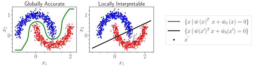
Figure 1: Investigating the accuracy and interpretability of our method. Left: The global decision boundary of our method that separates the classes correctly. Right: The local hyperplane pertaining to an example $x^{\prime}$ which, correctly classifies the local example and retains a good global classification for the neighboring points.

Initially, we investigate the global accuracy of our method. As shown in Figure 1 (left), our method correctly classifies all the examples. Furthermore, our method learns an optimal non-linear decision boundary that separates the classes (plotted in green). Lastly, in Figure 1 (right) we investigate the local interpretability of our method, by taking a point $x^{\prime}$ and calculating the corresponding weights $\left(\hat{w}\left(x^{\prime}\right),\hat{w}\left(x^{\prime}\right)_{0}\right)$ generated by our hypernetwork. The black line shows all the points that reside on the hyperplane $\hat{w}(x^{\prime})$ as $\{x\,|\,\hat{w}\left(x^{\prime}\right)^{T}\,x+\hat{w}_{0}\left(x^{\prime}\right)=0\}$. It is important to highlight that the local hyperplane does not only correctly classify the point $x^{\prime}$, but also the neighboring points, retaining an accurate linear classifier for the full training set. As a result, our model is globally accurate and non-linear (left), but also locally linear and explainable (right) at the same time.

3 Related Work

Interpretable Models by Design.

There exist Machine Learning models that offer interpretability by default. A standard approach is to use linear models [Tibshirani, 1996, Efron et al., 2004, Berkson, 1953] that assign interpretable weights to each of the input features. On the other hand, decision trees [Loh, 2011, Craven and Shavlik, 1995] use splitting rules that build up leaves and nodes. Every terminal node is associated with a predicted label, making it possible to follow the rules that led to a specific prediction. Bayesian methods such as Naive Bayes [Murphy et al., 2006] or Bayesian Neural Networks [Friedman et al., 1997] provide a framework for reasoning on the interactions of prior beliefs with evidence, thus simplifying the interpretation of probabilistic outputs. Instance based-models allow experts to reason about predictions based on the similarity to the train samples. The prediction model aggregates the labels of the neighbors in the training set, using the average of the top-k most similar samples [Freitas, 2014, Kim et al., 2015], or decision functions extracted from prototypes Martens et al. [2007]. However, these models trade-off the performance for the sake of interpretability, therefore challenging their usage on applications that need high performance.

Interpretable Model Distillation.

Given the common understanding that complex models are not interpretable, prior works propose to learn simple surrogates for mimicking the input-output behavior of the complex models [Burkart and Huber, 2021]. Such surrogate models are interpretable, such as linear regression or decision trees [Ribeiro et al., 2016]. The local surrogates generate interpretations only valid in the neighborhood of the selected samples. Some approaches explain the output by computing the contribution of each attribute [Lundberg and Lee, 2017] to the prediction of the particular sample. An alternative strategy is to fit globally interpretable models, by relying on decision trees [Frosst and Hinton, 2017, Yang et al., 2018], or linear models [Ribeiro et al., 2016]. Moreover, global explainers sometimes provide feature importances [Goldstein et al., 2015, Cortez and Embrechts, 2011], which can be used for auxiliary purposes such as feature engineering. Most of the surrogate models tackle the explainability task disjointly, by first training a black box model, then learning a surrogate in a second step.

Interpretable Deep Learning via Visualization.

Given the success of neural networks in real-world applications in computer vision, a series of prior works [Ras et al., 2022] introduce techniques aiming at explaining their predictions. A direct way to measure the feature importance is by evaluating the partial derivative of the network given the input [Simonyan et al., 2013]. CAM upscales the output of the last convolutional layers after applying Global Average Pooling (GAP), obtaining a map of the class activations used for interpretability  [Zhou et al., 2016]. DeepLift calculates pixel-wise relevance scores by computing differences with respect to a reference image  [Shrikumar et al., 2017]. Integrated Gradients use a baseline image to compute the cumulative sensibility of a black-box model $f$ to pixel-wise changes [Sundararajan et al., 2017]. Other methods directly compute the pixel-wise relevance scores such that the network’s output equals the sum of scores computed via Taylor Approximations [Montavon et al., 2017]. In another stream of works, perturbation-based methods offer interpretability by occluding a group of pixels on the black-box model [Zeiler and Fergus, 2014], or by adding a small amount of noise to the input of a surrogate model [Fong and Vedaldi, 2017]. Alternative approaches propose to compute the relevance of a specific input feature by marginalizing out the prediction of a probabilistic model [Zintgraf et al., 2017].

4 Experimental Protocol

4.1 Predictive Accuracy Experiments

Baselines: In terms of interpretable white-box classifiers, we compare against Logistic Regression and Decision Trees, based on their scikit-learn library implementations [Pedregosa et al., 2011]. On the other hand, we compare against two strong classifiers on tabular datasets, Random Forest and CatBoost. We use the scikit-learn interface for Random Forest, while for CatBoost we use the official implementation provided by the authors [Prokhorenkova et al., 2018]. Lastly, in terms of interpretable deep learning architectures, we compare against TabNet [Arik and Pfister, 2021], a transformer architecture that makes use of attention for instance-wise feature-selection.

Protocol: We run our predictive accuracy experiments on the AutoML benchmark that includes 35 diverse classification problems, containing between 690 and 539 383 data points, and between 5 and 7 201 features. For more details about the datasets included in our experiments, we point the reader to Appendix B. In our experiments, numerical features are standardized, while we transform categorical features through one-hot encoding. For binary classification datasets we use target encoding, where a category is encoded based on a shrunk estimate of the average target values for the data instances belonging to that category. In the case of missing values, we impute numerical features with zero and categorical features with a new category representing the missing value. For CatBoost and TabNet we do not encode categorical features since the algorithms natively handle them. For all the baselines we use the default hyperparameters offered by the respective libraries. For our method, we use the default hyperparameters that are suggested from a previous recent work [Kadra et al., 2021]. Lastly, as the evaluation metric we use the area under the ROC curve (AUROC). When reporting results, we use the mean over 10 repetitions for every method considered in the experiments.

4.2 Explainability Experiments

Baselines: First, we compare against Random, a baseline that generates random importance weights. Furthermore, BreakDown decomposes predictions into parts that can be attributed to certain features [Staniak and Biecek, 2018]. TabNet offers instance-wise feature importances by making use of attention. LIME is a local interpretability method [Ribeiro et al., 2016] that fits an explainable surrogate (local model) to single instance predictions of black-box models. On the other hand, L2X is a method that applies instance-wise feature selection via variational approximations of mutual information [Chen et al., 2018] by making use of a neural network to generate the weights of the explainer. MAPLE is a method that uses local linear modeling by exploring random forests as a feature selection method [Plumb et al., 2018]. SHAP is an additive feature attribution method [Lundberg and Lee, 2017] that allows local interpretation of the data instances. Last but not least, Kernel SHAP offers a reformulation of the LIME constrains [Lundberg and Lee, 2017].

Metrics: As explainability evaluation metrics we use faithfulness [Lundberg and Lee, 2017], monotonicity [Luss et al., 2021] (including the ROAR variants [Hooker et al., 2019]), infidelity [Yeh et al., 2019] and Shapley correlation [Lundberg and Lee, 2017]. For a detailed description of the metrics, we refer the reader to XAI-Bench, a recent explainability benchmark [Liu et al., 2021].

Protocol: For our explainability-related experiments, we use all three datasets (Gaussian Linear, Gaussian Non-Linear, and Gaussian Piecewise) available in the XAI-Bench [Liu et al., 2021]. For the state-of-the-art explainability baselines, we use the Tabular ResNet (TabResNet) backbone as the model for which the predictions are to be interpreted (same as for INN). We experiment with different versions of the datasets that feature diverse $\rho$ values, where $\rho$ corresponds to the amount of correlation among features. All datasets feature a train/validation set ratio of 10 to 1.

Implementation Details: We use PyTorch as the backbone library for implementing our method. As a backbone, we use a TabResNet where the convolutional layers are replaced with fully-connected layers as suggested by recent work [Kadra et al., 2021]. For our architecture, we use 2 residual blocks and 128 units per layer combined with the GELU activation [Hendrycks and Gimpel, 2016]. When training our network, we use snapshot ensembling [Huang et al., 2017] combined with cosine annealing with restarts [Loshchilov and Hutter, 2019]. We use a learning rate and weight decay value of 0.01, where, the learning rate is warmed up to 0.01 for the first 5 epochs. Our network is trained for 100 epochs with a batch size of 64. We make our implementation publicly available.

5 Experiments and Results

Hypothesis 1:

INN outperforms interpretable white-box models in terms of predictive accuracy.

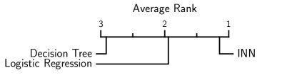
Figure 2: The critical difference diagram for the white-box interpretable methods. A lower rank indicates a better performance over datasets.

We compare our method against decision trees and logistic regression, two white-box interpretable models. We run all aforementioned methods on the AutoML benchmark and we measure the predictive performance in terms of AUROC. Lastly, we measure the statistical significance of the results using the Wilcoxon-Holm test [Demšar, 2006].

Figure 2 shows that INN achieves the best rank across the AutoML benchmark datasets. Furthermore, the difference is statistically significant against both decision trees ($p=2.9\times 10^{-7}$) and logistic regression ($p=1.8\times 10^{-5}$). The detailed per-dataset results are presented in Appendix B.

Hypothesis 2:

The explainability of INN does not have a negative impact on predictive accuracy. Additionally, it achieves a comparable performance against state-of-the-art methods.

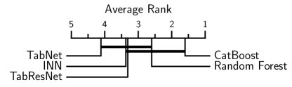
Figure 3: Black-box methods comparison. Critical difference diagram indicating the ranks over all datasets. A lower rank indicates a better performance. Connected ranks via a bold bar indicate that performances are not significantly different ($p>0.05$).

This experiment addresses a simple question "Is our explainable neural network as accurate as a black-box neural network counterpart, that has the same architecture and same capacity?". Since our hypernetwork $g(x;\theta)$ is a slight modification of the TabResNet Kadra et al. [2021], we compare it against TabResNet as a classifier. For completeness, we also compare against three other strong baselines, Gradient-Boosted Decision Trees (CatBoost), TabNet, and Random Forest.

Table 1: Investigating the interpretability of INNs against state-of-the-art interpretability methods. The results are generated from the XAI Benchmark [Liu et al., 2021] datasets (with $\rho=0$).

Metric Dataset Random Breakd. Maple LIME L2X SHAP K. SHAP TabNet INN Faithfulness $\left(\uparrow\right)$ Gaussian Linear 0.004 0.645 0.980 0.882 0.010 0.974 0.981 0.138 0.987 Gaussian Non-Linear -0.079 -0.001 0.487 0.796 0.155 0.926 0.970 0.161 0.621 Gaussian Piecewise 0.091 0.634 0.967 0.929 0.016 0.981 0.990 0.058 0.841 Faithfulness (ROAR) $\left(\uparrow\right)$ Gaussian Linear -0.039 0.494 0.548 0.544 0.049 0.549 0.550 0.041 0.639 Gaussian Non-Linear 0.050 0.006 0.040 -0.040 -0.060 -0.010 -0.036 -0.001 0.027 Gaussian Piecewise -0.055 0.372 0.347 0.450 0.015 0.409 0.426 0.072 0.404 Infidelity $\left(\downarrow\right)$ Gaussian Linear 0.219 0.041 0.007 0.007 0.034 0.007 0.007 0.049 0.007 Gaussian Non-Linear 0.075 0.086 0.021 0.071 0.089 0.030 0.022 0.047 0.018 Gaussian Piecewise 0.132 0.047 0.014 0.019 0.070 0.016 0.019 0.046 0.008 Monotonicity (ROAR) $\left(\uparrow\right)$ Gaussian Linear 0.487 0.605 0.700 0.652 0.437 0.680 0.667 0.585 0.785 Gaussian Non-Linear 0.497 0.542 0.645 0.587 0.457 0.670 0.632 0.493 0.637 Gaussian Piecewise 0.485 0.665 0.787 0.427 0.442 0.717 0.797 0.542 0.682 Shapley Correlation $\left(\uparrow\right)$ Gaussian Linear -0.016 0.246 0.999 0.942 -0.214 0.993 0.999 0.095 0.999 Gaussian Non-Linear -0.069 -0.179 0.686 0.872 -0.095 0.974 0.999 0.125 0.741 Gaussian Piecewise -0.078 0.099 0.983 0.959 0.157 0.991 0.999 0.070 0.875 Total Wins 1 0 2 2 0 2 7 0 7

The results of Figure 3 demonstrate that INN achieves almost the same performance as TabResNet, while outperforming TabNet, indicating that its explainability does not harm accuracy. There is no statistical significance of the differences between INN, TabResNet and TabNet. Furthermore, both INN and TabResNet demand approximately the same training time, where, the INN runtime is slower by a factor of only 0.04 $\pm$ 0.03% across datasets. As a result, the explainability of our method comes as a free-lunch benefit.

Furthermore, our method is competitive against state-of-the-art black-box models, such as CatBoost and Random Forest. Although INN has a worse rank, the difference is not statistically significant. To further investigate the results on individual datasets, in Figure 5 we plot the distribution of the gains in performance of all methods over a single decision tree model. The results indicate that all methods achieve a comparable gain in performance across the AutoML benchmark datasets. We present detailed results in Appendix B.

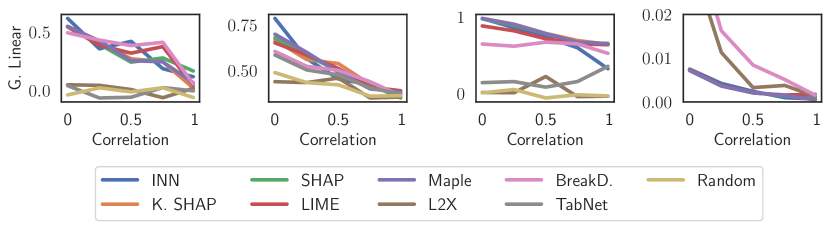
Figure 4: Performance analysis of different interpretability methods over a varying degree of feature correlation $\rho$. We present the performance of all methods on faithfulness (ROAR), monotonicity (ROAR), faithfulness and infidelity on the Gaussian Linear dataset for $\rho$ values ranging from [0, 1].

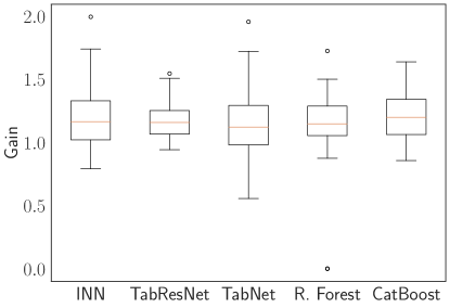
Figure 5: The gain distribution of the state-of-the-art models is calculated by dividing the test AUROC against the test AUROC of a decision tree.

Hypothesis 3:

INNs offer competitive levels of interpretability compared to state-of-the-art explainer techniques.

We compare against 8 explainer baselines in terms of 5 explainability metrics in the 3 datasets of the XAI benchmark [Liu et al., 2021], following the protocol we detailed in Section 4.2.

The results of Table 1 demonstrate that INN is competitive against all explainers across the indicated interpretability metrics. We tie in performance with the second-best method Kernel-SHAP [Lundberg and Lee, 2017] and perform strongly against the other explainers. It is worth highlighting that in comparison to all the explainer techniques, the interpretability of our method comes as a free-lunch. In contrast, all the rival methods except TabNet are surrogate interpretable models to black-box models.

As a result, for all surrogate interpretable baselines we first need to train a black-box TabResNet model. Then, for the prediction of every data point, we additionally train a local explainer around that point by predicting with the black-box model multiple times. In stark contrast, our method combines prediction models and explainers as an all-in-one neural network. To generate an explainable model for a data point $x_{n}$, INN does not need to train a per-point explainer. Instead, INN requires only a forward pass through the hypernetwork $g(x_{n};\theta)$ to generate a linear explainer. Moreover, INN strongly outperforms TabNet, the other baseline that offers explainability by design, achieving both better interpretability (Table 1) and better accuracy (Figure 3).

Lastly, we compare all interpretability methods on 4 out of 5 metrics in the presence of a varying $\rho$ factor, which controls the correlation of features on the Gaussian Linear dataset. Figure 4, presents the comparison, where INN behaves similarly to other interpretable methods and has a comparable performance with the top-methods in the majority of metrics. The results agree with the findings of prior work [Liu et al., 2021], where performance drops in the presence of feature correlations.

Hypothesis 4:

INN offers a global (dataset-wide) interpretability of feature importances.

Table 2: The feature rank importances for the Census dataset features from the different methods. A lower rank is associated with a higher feature importance.

Feature SHAP Decision Tree TabNet CatBoost INN Age 2 5 2 3 3 Capital Gain 9 4 3 1 1 Capital Loss 10 9 14 4 5 Demographic 1 2 9 10 6 Education 5 3 5 9 9 Education num. 4 12 6 6 2 Hours per week 6 7 7 7 4 Race 8 10 5 12 7 Occupation 3 6 8 8 10 Relationship 7 1 1 2 8

The purpose of this experiment is to showcase that INN can be used to analyze the global interpretability of feature attributions, where the dataset-wide importance of the $m$-th feature is aggregated as $\frac{1}{N}\sum_{n=1}^{N}|\hat{w}(x_{n};\theta)_{m}\,x_{n,m}|$. Since we are not aware of a public benchmark offering ground-truth global interpretability of features, we experiment with the Adult Census Income [Kohavi et al., 1996], a very popular dataset, where the goal is to predict whether income exceeds $50K/yr based on census data. We consider Decision Trees, CatBoost, TabNet and INN as explainable methods. Additionally, we use SHAP to explain the predictions of the TabResNet backbone.

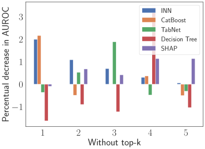
Figure 6: Investigating the decrease in AUROC when removing the $k$-th most important feature.

We present the importances that the different methods assign to features in Table 2. To verify the feature rankings generated by the rival models, we analyze the top-5 features of every individual method by investigating the drop in model performance if we remove the feature. The more important a feature is, the more accuracy should drop when removing that feature. The results of Figure 6 show that INNs have a higher relative drop in the model’s accuracy when the most important predicted feature is removed. This shows that the feature ranking generated by INN is proportional to the predictive importance of the feature and monotonously decreasing. In contrast, in the case of CatBoost, TabNet, SHAP, and decision trees, the decrease in accuracy is not proportional to the order of the feature importance (e.g. the case of Top-1 for Decision Tree, TabNet, SHAP or Top-2 for Catboost).

Hypothesis 5:

INN can be extended to image classification backbones.

We use INN to explain the predictions of ResNet50, a broadly used computer vision backbone. We take the pre-trained backbone $\phi(\cdot):\mathrm{R}^{H\times W\times K}\rightarrow\mathrm{R}^{D}$ from PyTorch and change the output layer to a fully-connected layer $w:\mathrm{R}^{D}\rightarrow\mathrm{R}^{H\times W\times K\times C}$ that generates the weights for multiplying the input image $x\in\mathrm{R}^{H\times W\times K}$ with $K$ channels, and finally obtain the logits $z_{c}$ for the class $c$. In this experiment, we use $\lambda=10^{-3}$ as the L1 penalty strength.

We fine-tuned the ImageNet pre-trained ResNet50 models, both for the explainable (INN-ResNet) and the black-box (ResNet) variants for 400 epochs on the CIFAR-10 dataset with a learning rate of $10^{-4}$. To test whether the explainable variant is as accurate as the black-box model, we evaluate the validation accuracy after 5 independent training runs. INN-ResNet achieves an accuracy of $87.49\pm 1.73$ and the ResNet $88.76\pm 1.50$, with the difference being statistically insignificant.

We compare our method to the following image explainability baselines: Saliency Maps (Gradients) Simonyan et al. [2013], DeepLift Shrikumar et al. [2017], Integrated Gradients Ancona et al. [2017] with SmoothGrad. All of the baselines are available via the captum library. We compare the rival explainers to INN-ResNet by visually interpreting the pixel-wise weights of selected images in Figure 7. The results confirm that INN-ResNet generates higher weights for pixel regions that include descriptive parts of the object.

Figure 7: Comparison of INN against explainability techniques for image classification.

6 Conclusion

In this work, we propose explainable deep networks that are not only as accurate as their black-box counterparts but also as interpretable as state-of-the-art explanation techniques. With extensive experiments, we show that the explainable deep learning networks outperform traditional white-box models in terms of performance. Moreover, the experiments confirm that the explainable deep-learning architecture does not include a degradation in performance or an overhead on time compared to the plain black-box counterpart, achieving competitive results against state-of-the-art classifiers in tabular data. Our method matches competitive state-of-the-art explainability methods on a recent explainability benchmark in tabular data, and on image data such as CIFAR-10, offering explanations of predictions as a free lunch.

Appendix A Plots

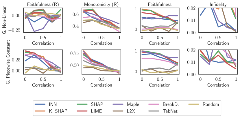
Figure 8: Performance analysis of all explainable methods on faithfulness (ROAR), monotonicity (ROAR), faithfulness, and infidelity. The results are shown for the Gaussian Non-Linear Additive and Gaussian Piecewise datasets where, correlation ($\rho$) ranges from [0, 1].

In Figure 8, we present the performance of the different explainers for the different explainability metrics. We present results for the Gaussian Non-Linear Additive and Gaussian Piecewise Constant datasets over a varying presence of correlation $\rho$ between the features. The results show that our method achieves competitive results against Kernel Shap (K. SHAP) and LIME, the strongest baselines.

Appendix B Tables

To describe the 35 datasets present in our accuracy-related experiments, we summarize the main descriptive statistics in Table 3. The statistics show that our datasets are diverse, covering both binary and multi-class classification problems with imbalanced and balanced datasets that contain a diverse number of features and examples.

Additionally, we provide the per-dataset performances for the accuracy-related experiments of every method. Table 5 summarizes the performances on the train split, where, as observed Random Forest and decision trees overfit the training data excessively compared to the other methods. Lastly, Table 4 provides the performance of every method on the test split, where, INN, TabResNet, CatBoost, and Random Forest achieve similar performances.

Table 3: Statistics regarding the AutoML benchmark datasets.

Dataset ID Dataset Name Number of Instances Number of Features Number of Classes Majority Class Percentage Minority Class Percentage 3 kr-vs-kp 3196 37 2 52.222 47.778 12 mfeat-factors 2000 217 10 10.000 10.000 31 credit-g 1000 21 2 70.000 30.000 54 vehicle 846 19 4 25.768 23.522 1067 kc1 2109 22 2 84.542 15.458 1111 KDDCup09 appetency 50000 231 2 98.220 1.780 1169 airlines 539383 8 2 55.456 44.544 1461 bank-marketing 45211 17 2 88.302 11.698 1464 blood-transfusion-service-center 748 5 2 76.203 23.797 1468 cnae-9 1080 857 9 11.111 11.111 1486 nomao 34465 119 2 71.438 28.562 1489 phoneme 5404 6 2 70.651 29.349 1590 adult 48842 15 2 76.072 23.928 4135 Amazon employee access 32769 10 2 94.211 5.789 23512 higgs 98050 29 2 52.858 47.142 23517 numerai28.6 96320 22 2 50.517 49.483 40685 shuttle 58000 10 7 78.597 0.017 40981 Australian 690 15 2 55.507 44.493 40984 segment 2310 20 7 14.286 14.286 40996 Fashion-MNIST 70000 785 10 10.000 10.000 41027 jungle chess 44819 7 3 51.456 9.672 41138 APSFailure 76000 171 2 98.191 1.809 41142 christine 5418 1637 2 50.000 50.000 41143 jasmine 2984 145 2 50.000 50.000 41146 sylvine 5124 21 2 50.000 50.000 41147 albert 425240 79 2 50.000 50.000 41150 MiniBooNE 130064 51 2 71.938 28.062 41159 guillermo 20000 4297 2 59.985 40.015 41161 riccardo 20000 4297 2 75.000 25.000 41163 dilbert 10000 2001 5 20.490 19.130 41164 fabert 8237 801 7 23.394 6.094 41165 robert 10000 7201 10 10.430 9.580 41166 volkert 58310 181 10 21.962 2.334 41168 jannis 83733 55 4 46.006 2.015 41169 helena 65196 28 100 6.143 0.170

Table 4: The per-dataset test AUROC performance for all methods in the accuracy-experiments. The test performance is the mean value from 10 runs with different seeds. A value of -1 represents a failure of running on that particular dataset.

Dataset ID Decision Tree Logistic Regression Random Forest TabNet TabResNet CatBoost INN 3 0.987 0.990 0.998 0.983 0.998 0.999 0.998 12 0.938 0.999 0.998 0.995 0.999 0.999 0.999 31 0.643 0.775 0.795 0.511 0.781 0.790 0.780 54 0.804 0.938 0.927 0.501 0.963 0.934 0.963 1067 0.620 0.802 0.801 0.789 0.801 0.800 0.802 1111 0.535 0.816 0.793 -1.000 0.760 0.843 0.763 1169 0.592 0.679 0.692 0.699 0.684 0.718 0.684 1461 0.703 0.908 0.930 0.926 0.911 0.937 0.910 1464 0.599 0.749 0.666 0.516 0.752 0.709 0.754 1468 0.926 0.996 0.995 0.495 0.993 0.996 0.995 1486 0.935 0.987 0.993 0.991 0.988 0.994 0.988 1489 0.842 0.805 0.962 0.928 0.897 0.948 0.895 1590 0.752 0.903 0.917 0.908 0.906 0.930 0.906 4135 0.639 0.853 0.846 -1.000 0.855 0.883 0.855 23512 0.626 0.683 0.794 0.803 0.752 0.804 0.750 23517 0.501 0.530 0.515 0.522 0.529 0.526 0.528 40685 0.967 0.994 1.000 0.986 1.000 -1.000 0.999 40981 0.817 0.930 0.945 0.463 0.929 0.935 0.927 40984 0.946 0.980 0.995 0.985 0.990 0.995 0.990 40996 0.886 0.984 0.991 0.989 0.984 0.993 0.984 41027 0.792 0.797 0.931 0.976 0.956 0.974 0.955 41138 0.861 0.974 0.989 0.970 0.990 0.992 0.990 41142 0.626 0.742 0.796 0.713 0.783 0.822 0.785 41143 0.749 0.850 0.880 0.823 0.870 0.870 0.871 41146 0.910 0.966 0.983 0.974 0.979 0.988 0.979 41147 0.606 0.748 0.762 -1.000 0.751 0.779 0.751 41150 0.867 0.938 0.981 0.896 0.939 0.984 0.938 41159 0.730 0.712 0.892 0.754 0.716 0.897 0.716 41161 0.857 0.995 0.999 0.997 0.998 1.000 0.998 41163 0.873 0.994 0.999 0.998 0.997 1.000 0.997 41164 0.786 0.898 0.925 0.888 0.910 0.935 0.911 41165 0.579 0.748 0.835 0.788 0.785 0.895 0.786 41166 0.699 0.882 0.927 0.918 0.907 0.949 0.908 41168 0.633 0.798 0.831 0.813 0.838 0.862 0.837 41169 0.554 0.841 0.800 0.842 0.855 0.866 0.855

Table 5: The per-dataset train AUROC performance for all methods in the accuracy-experiments. The train performance is the mean value from 10 runs with different seeds. A value of -1 represents a failure of running on that particular dataset.

Dataset ID Decision Tree Logistic Regression Random Forest TabNet TabResNet CatBoost INN 3 1.000 0.990 1.000 0.980 0.997 1.000 0.999 12 1.000 1.000 1.000 1.000 0.996 1.000 1.000 31 1.000 0.795 1.000 0.514 0.880 0.963 0.926 54 1.000 0.955 1.000 0.492 0.962 1.000 0.982 1067 0.998 0.818 0.997 0.825 0.824 0.971 0.827 1111 1.000 0.822 1.000 -1.000 0.790 0.899 0.822 1169 0.994 0.680 0.994 0.705 0.680 0.733 0.685 1461 1.000 0.908 1.000 0.947 0.906 0.948 0.910 1464 0.983 0.757 0.978 0.490 0.773 0.934 0.784 1468 1.000 1.000 1.000 0.493 0.988 1.000 0.998 1486 1.000 0.988 1.000 0.995 0.984 0.997 0.989 1489 1.000 0.813 1.000 0.947 0.899 0.982 0.909 1590 1.000 0.903 1.000 0.920 0.904 0.935 0.907 4135 1.000 0.839 0.998 -1.000 0.842 0.981 0.844 23512 1.000 0.683 1.000 0.820 0.727 0.831 0.752 23517 1.000 0.533 1.000 0.529 0.522 0.703 0.529 40685 1.000 0.999 1.000 0.988 0.894 -1.000 0.977 40981 1.000 0.932 1.000 0.472 0.964 0.996 0.979 40984 1.000 0.983 1.000 0.990 0.963 1.000 0.983 40996 1.000 0.989 1.000 0.997 0.956 0.999 0.960 41027 1.000 0.799 1.000 0.980 0.916 0.989 0.926 41138 1.000 0.992 1.000 0.999 0.990 1.000 0.993 41142 1.000 0.942 1.000 0.951 0.929 0.999 1.000 41143 1.000 0.868 1.000 0.874 0.888 0.992 0.922 41146 1.000 0.967 1.000 0.989 0.976 1.000 0.982 41147 1.000 0.746 1.000 -1.000 0.740 0.827 0.751 41150 1.000 0.938 1.000 0.896 0.947 0.988 0.970 41159 1.000 0.826 1.000 0.840 0.714 0.977 0.812 41161 1.000 1.000 1.000 0.999 0.975 1.000 0.998 41163 1.000 1.000 1.000 1.000 0.967 1.000 0.984 41164 1.000 0.994 1.000 0.968 0.954 0.983 0.986 41165 1.000 1.000 1.000 0.876 0.869 1.000 0.971 41166 1.000 0.889 1.000 0.943 0.858 0.992 0.872 41168 1.000 0.804 1.000 0.911 0.813 0.971 0.839 41169 1.000 0.854 1.000 0.867 0.655 0.998 0.668

References

- Alvarez-Melis and Jaakkola [2018] David Alvarez-Melis and Tommi S. Jaakkola. Towards robust interpretability with self-explaining neural networks. In Proceedings of the 32nd International Conference on Neural Information Processing Systems, NIPS’18, page 7786–7795, Red Hook, NY, USA, 2018. Curran Associates Inc.
- Ancona et al. [2017] Marco Ancona, Enea Ceolini, Cengiz Öztireli, and Markus Gross. Towards better understanding of gradient-based attribution methods for deep neural networks. arXiv preprint arXiv:1711.06104, 2017.
- Arik and Pfister [2021] Sercan Ö Arik and Tomas Pfister. Tabnet: Attentive interpretable tabular learning. In Proceedings of the AAAI Conference on Artificial Intelligence, volume 35, pages 6679–6687, 2021.
- Berkson [1953] Joseph Berkson. A statistically precise and relatively simple method of estimating the bio-assay with quantal response, based on the logistic function. Journal of the American Statistical Association, 48(263):565–599, 1953.
- Burkart and Huber [2021] Nadia Burkart and Marco F Huber. A survey on the explainability of supervised machine learning. Journal of Artificial Intelligence Research, 70:245–317, 2021.
- Chen et al. [2018] Jianbo Chen, Le Song, Martin Wainwright, and Michael Jordan. Learning to explain: An information-theoretic perspective on model interpretation. In Jennifer Dy and Andreas Krause, editors, Proceedings of the 35th International Conference on Machine Learning, volume 80 of Proceedings of Machine Learning Research, pages 883–892. PMLR, 10–15 Jul 2018. URL https://proceedings.mlr.press/v80/chen18j.html.
- Cortez and Embrechts [2011] Paulo Cortez and Mark J. Embrechts. Opening black box data mining models using sensitivity analysis. In Proceedings of the IEEE Symposium on Computational Intelligence and Data Mining, CIDM 2011, part of the IEEE Symposium Series on Computational Intelligence 2011, April 11-15, 2011, Paris, France, pages 341–348. IEEE, 2011. doi: 10.1109/CIDM.2011.5949423. URL https://doi.org/10.1109/CIDM.2011.5949423.
- Craven and Shavlik [1995] Mark Craven and Jude Shavlik. Extracting tree-structured representations of trained networks. Advances in neural information processing systems, 8, 1995.
- Demšar [2006] Janez Demšar. Statistical comparisons of classifiers over multiple data sets. J. Mach. Learn. Res., 7:1–30, December 2006. ISSN 1532-4435. URL http://dl.acm.org/citation.cfm?id=1248547.1248548.
- Efron et al. [2004] Bradley Efron, Trevor Hastie, Iain Johnstone, and Robert Tibshirani. Least angle regression. The Annals of Statistics, 32(2):407 – 499, 2004. doi: 10.1214/009053604000000067. URL https://doi.org/10.1214/009053604000000067.
- Fong and Vedaldi [2017] Ruth C. Fong and Andrea Vedaldi. Interpretable explanations of black boxes by meaningful perturbation. In IEEE International Conference on Computer Vision, ICCV 2017, Venice, Italy, October 22-29, 2017, pages 3449–3457. IEEE Computer Society, 2017. doi: 10.1109/ICCV.2017.371. URL https://doi.org/10.1109/ICCV.2017.371.
- Freitas [2014] Alex A Freitas. Comprehensible classification models: a position paper. ACM SIGKDD explorations newsletter, 15(1):1–10, 2014.
- Friedman et al. [1997] Nir Friedman, Dan Geiger, and Moises Goldszmidt. Bayesian network classifiers. Machine learning, 29:131–163, 1997.
- Frosst and Hinton [2017] Nicholas Frosst and Geoffrey E. Hinton. Distilling a neural network into a soft decision tree. In Tarek R. Besold and Oliver Kutz, editors, Proceedings of the First International Workshop on Comprehensibility and Explanation in AI and ML 2017 co-located with 16th International Conference of the Italian Association for Artificial Intelligence (AI*IA 2017), Bari, Italy, November 16th and 17th, 2017, volume 2071 of CEUR Workshop Proceedings. CEUR-WS.org, 2017. URL https://ceur-ws.org/Vol-2071/CExAIIA_2017_paper_3.pdf.
- Gijsbers et al. [2019] P. Gijsbers, E. LeDell, S. Poirier, J. Thomas, B. Bischl, and J. Vanschoren. An open source automl benchmark. arXiv preprint arXiv:1907.00909 [cs.LG], 2019. URL https://arxiv.org/abs/1907.00909. Accepted at AutoML Workshop at ICML 2019.
- Goldstein et al. [2015] Alex Goldstein, Adam Kapelner, Justin Bleich, and Emil Pitkin. Peeking inside the black box: Visualizing statistical learning with plots of individual conditional expectation. journal of Computational and Graphical Statistics, 24(1):44–65, 2015.
- Gulum et al. [2021] Mehmet A Gulum, Christopher M Trombley, and Mehmed Kantardzic. A review of explainable deep learning cancer detection models in medical imaging. Applied Sciences, 11(10):4573, 2021.
- Ha et al. [2017] David Ha, Andrew M. Dai, and Quoc V. Le. Hypernetworks. In International Conference on Learning Representations, 2017. URL https://openreview.net/forum?id=rkpACe1lx.
- Hendrycks and Gimpel [2016] Dan Hendrycks and Kevin Gimpel. Gaussian error linear units (gelus). arXiv preprint arXiv:1606.08415, 2016.
- Hooker et al. [2019] Sara Hooker, Dumitru Erhan, Pieter-Jan Kindermans, and Been Kim. A Benchmark for Interpretability Methods in Deep Neural Networks. Curran Associates Inc., Red Hook, NY, USA, 2019.
- Huang et al. [2017] Gao Huang, Yixuan Li, Geoff Pleiss, Zhuang Liu, John E. Hopcroft, and Kilian Q. Weinberger. Snapshot ensembles: Train 1, get m for free. In International Conference on Learning Representations, 2017. URL https://openreview.net/forum?id=BJYwwY9ll.
- Kadra et al. [2021] Arlind Kadra, Marius Lindauer, Frank Hutter, and Josif Grabocka. Well-tuned simple nets excel on tabular datasets. In Thirty-Fifth Conference on Neural Information Processing Systems, 2021.
- Kim et al. [2015] Been Kim, Julie A Shah, and Finale Doshi-Velez. Mind the gap: A generative approach to interpretable feature selection and extraction. Advances in neural information processing systems, 28, 2015.
- Kohavi et al. [1996] Ron Kohavi et al. Scaling up the accuracy of naive-bayes classifiers: A decision-tree hybrid. In Kdd, volume 96, pages 202–207, 1996.
- Liu et al. [2021] Yang Liu, Sujay Khandagale, Colin White, and Willie Neiswanger. Synthetic benchmarks for scientific research in explainable machine learning. In Advances in Neural Information Processing Systems Datasets Track, 2021.
- Loh [2011] Wei-Yin Loh. Classification and regression trees. Wiley interdisciplinary reviews: data mining and knowledge discovery, 1(1):14–23, 2011.
- Loshchilov and Hutter [2019] Ilya Loshchilov and Frank Hutter. Decoupled weight decay regularization. In International Conference on Learning Representations, 2019. URL https://openreview.net/forum?id=Bkg6RiCqY7.
- Lundberg and Lee [2017] Scott M. Lundberg and Su-In Lee. A unified approach to interpreting model predictions. In Isabelle Guyon, Ulrike von Luxburg, Samy Bengio, Hanna M. Wallach, Rob Fergus, S. V. N. Vishwanathan, and Roman Garnett, editors, Advances in Neural Information Processing Systems 30: Annual Conference on Neural Information Processing Systems 2017, December 4-9, 2017, Long Beach, CA, USA, pages 4765–4774, 2017. URL https://proceedings.neurips.cc/paper/2017/hash/8a20a8621978632d76c43dfd28b67767-Abstract.html.
- Luss et al. [2021] Ronny Luss, Pin-Yu Chen, Amit Dhurandhar, Prasanna Sattigeri, Yunfeng Zhang, Karthikeyan Shanmugam, and Chun-Chen Tu. Leveraging latent features for local explanations. In Proceedings of the 27th ACM SIGKDD Conference on Knowledge Discovery and Data Mining, KDD ’21, page 1139–1149, New York, NY, USA, 2021. Association for Computing Machinery. ISBN 9781450383325. doi: 10.1145/3447548.3467265. URL https://doi.org/10.1145/3447548.3467265.
- Martens et al. [2007] David Martens, Bart Baesens, Tony Van Gestel, and Jan Vanthienen. Comprehensible credit scoring models using rule extraction from support vector machines. Eur. J. Oper. Res., 183(3):1466–1476, 2007. doi: 10.1016/j.ejor.2006.04.051. URL https://doi.org/10.1016/j.ejor.2006.04.051.
- Montavon et al. [2017] Grégoire Montavon, Sebastian Lapuschkin, Alexander Binder, Wojciech Samek, and Klaus-Robert Müller. Explaining nonlinear classification decisions with deep taylor decomposition. Pattern Recognit., 65:211–222, 2017. doi: 10.1016/j.patcog.2016.11.008. URL https://doi.org/10.1016/j.patcog.2016.11.008.
- Murphy et al. [2006] Kevin P Murphy et al. Naive bayes classifiers. University of British Columbia, 18(60):1–8, 2006.
- Pedregosa et al. [2011] Gaël Pedregosa, Fabian acnd Varoquaux, Alexandre Gramfort, Vincent Michel, Bertrand Thirion, Olivier Grisel, Mathieu Blondel, Peter Prettenhofer, Ron Weiss, Vincent Dubourg, et al. Scikit-learn: Machine learning in python. the Journal of machine Learning research, 12:2825–2830, 2011.
- Plumb et al. [2018] Gregory Plumb, Denali Molitor, and Ameet S Talwalkar. Model agnostic supervised local explanations. Advances in neural information processing systems, 31, 2018.
- Prokhorenkova et al. [2018] Liudmila Prokhorenkova, Gleb Gusev, Aleksandr Vorobev, Anna Veronika Dorogush, and Andrey Gulin. Catboost: unbiased boosting with categorical features. Advances in neural information processing systems, 31, 2018.
- Ras et al. [2022] Gabrielle Ras, Ning Xie, Marcel van Gerven, and Derek Doran. Explainable deep learning: A field guide for the uninitiated. J. Artif. Intell. Res., 73:329–396, 2022. doi: 10.1613/jair.1.13200. URL https://doi.org/10.1613/jair.1.13200.
- Ribeiro et al. [2016] Marco Tulio Ribeiro, Sameer Singh, and Carlos Guestrin. "why should i trust you?": Explaining the predictions of any classifier. In Proceedings of the 22nd ACM SIGKDD International Conference on Knowledge Discovery and Data Mining, KDD ’16, page 1135–1144, New York, NY, USA, 2016. Association for Computing Machinery. ISBN 9781450342322. doi: 10.1145/2939672.2939778. URL https://doi.org/10.1145/2939672.2939778.
- Sadhwani et al. [2020] Apaar Sadhwani, Kay Giesecke, and Justin Sirignano. Deep Learning for Mortgage Risk*. Journal of Financial Econometrics, 19(2):313–368, 07 2020. ISSN 1479-8409. doi: 10.1093/jjfinec/nbaa025. URL https://doi.org/10.1093/jjfinec/nbaa025.
- Shrikumar et al. [2017] Avanti Shrikumar, Peyton Greenside, and Anshul Kundaje. Learning important features through propagating activation differences. In Doina Precup and Yee Whye Teh, editors, Proceedings of the 34th International Conference on Machine Learning, ICML 2017, Sydney, NSW, Australia, 6-11 August 2017, volume 70 of Proceedings of Machine Learning Research, pages 3145–3153. PMLR, 2017. URL http://proceedings.mlr.press/v70/shrikumar17a.html.
- Simonyan et al. [2013] Karen Simonyan, Andrea Vedaldi, and Andrew Zisserman. Deep inside convolutional networks: Visualising image classification models and saliency maps. arXiv preprint arXiv:1312.6034, 2013.
- Staniak and Biecek [2018] Mateusz Staniak and Przemyslaw Biecek. Explanations of model predictions with live and breakdown packages. arXiv preprint arXiv:1804.01955, 2018.
- Sundararajan et al. [2017] Mukund Sundararajan, Ankur Taly, and Qiqi Yan. Axiomatic attribution for deep networks. In Doina Precup and Yee Whye Teh, editors, Proceedings of the 34th International Conference on Machine Learning, ICML 2017, Sydney, NSW, Australia, 6-11 August 2017, volume 70 of Proceedings of Machine Learning Research, pages 3319–3328. PMLR, 2017. URL http://proceedings.mlr.press/v70/sundararajan17a.html.
- Tibshirani [1996] Robert Tibshirani. Regression shrinkage and selection via the lasso. Journal of the Royal Statistical Society: Series B (Methodological), 58(1):267–288, 1996.
- Tjoa and Guan [2021] Erico Tjoa and Cuntai Guan. A survey on explainable artificial intelligence (xai): Toward medical xai. IEEE Transactions on Neural Networks and Learning Systems, 32(11):4793–4813, 2021. doi: 10.1109/TNNLS.2020.3027314.
- Yang et al. [2018] Chengliang Yang, Anand Rangarajan, and Sanjay Ranka. Global model interpretation via recursive partitioning. In 20th IEEE International Conference on High Performance Computing and Communications; 16th IEEE International Conference on Smart City; 4th IEEE International Conference on Data Science and Systems, HPCC/SmartCity/DSS 2018, Exeter, United Kingdom, June 28-30, 2018, pages 1563–1570. IEEE, 2018. doi: 10.1109/HPCC/SmartCity/DSS.2018.00256. URL https://doi.org/10.1109/HPCC/SmartCity/DSS.2018.00256.
- Yeh et al. [2019] Chih-Kuan Yeh, Cheng-Yu Hsieh, Arun Sai Suggala, David I. Inouye, and Pradeep Ravikumar. On the (in)Fidelity and Sensitivity of Explanations. Curran Associates Inc., Red Hook, NY, USA, 2019.
- Zeiler and Fergus [2014] Matthew D. Zeiler and Rob Fergus. Visualizing and understanding convolutional networks. In David J. Fleet, Tomás Pajdla, Bernt Schiele, and Tinne Tuytelaars, editors, Computer Vision - ECCV 2014 - 13th European Conference, Zurich, Switzerland, September 6-12, 2014, Proceedings, Part I, volume 8689 of Lecture Notes in Computer Science, pages 818–833. Springer, 2014. doi: 10.1007/978-3-319-10590-1\_53. URL https://doi.org/10.1007/978-3-319-10590-1_53.
- Zhou et al. [2016] Bolei Zhou, Aditya Khosla, Àgata Lapedriza, Aude Oliva, and Antonio Torralba. Learning deep features for discriminative localization. In 2016 IEEE Conference on Computer Vision and Pattern Recognition, CVPR 2016, Las Vegas, NV, USA, June 27-30, 2016, pages 2921–2929. IEEE Computer Society, 2016. doi: 10.1109/CVPR.2016.319. URL https://doi.org/10.1109/CVPR.2016.319.
- Zintgraf et al. [2017] Luisa M. Zintgraf, Taco S. Cohen, Tameem Adel, and Max Welling. Visualizing deep neural network decisions: Prediction difference analysis. In 5th International Conference on Learning Representations, ICLR 2017, Toulon, France, April 24-26, 2017, Conference Track Proceedings. OpenReview.net, 2017. URL https://openreview.net/forum?id=BJ5UeU9xx.