Gradient Descent Monotonically Decreases the Sharpness of
Gradient Flow Solutions in Scalar Networks and Beyond

Abstract

Recent research shows that when Gradient Descent (GD) is applied to neural networks, the loss almost never decreases monotonically. Instead, the loss oscillates as gradient descent converges to its “Edge of Stability” (EoS). Here, we find a quantity that does decrease monotonically throughout GD training: the sharpness attained by the gradient flow solution (GFS)—the solution that would be obtained if, from now until convergence, we train with an infinitesimal step size. Theoretically, we analyze scalar neural networks with the squared loss, perhaps the simplest setting where the EoS phenomena still occur. In this model, we prove that the GFS sharpness decreases monotonically. Using this result, we characterize settings where GD provably converges to the EoS in scalar networks. Empirically, we show that GD monotonically decreases the GFS sharpness in a squared regression model as well as practical neural network architectures.

1 Introduction

The conventional analysis of gradient descent (GD) for smooth functions assumes that its step size $\eta$ is sufficiently small so that the loss decreases monotonically in each step. In particular, $\eta$ should be such that the loss sharpness (i.e., the maximum eigenvalue of its Hessian) is no more than $\frac{2}{\eta}$ for the entire GD trajectory. Such assumption is prevalent when analyzing GD in the context of general functions (e.g., Lee et al., 2016), and even smaller steps sizes are used in theoretical analyses of GD in neural networks (e.g., Du et al., 2019; Arora et al., 2019; Elkabetz & Cohen, 2021).

However, recent empirical work (Cohen et al., 2021; Wu et al., 2018; Xing et al., 2018; Gilmer et al., 2022) reveals that the descent assumption often fails to hold when applying GD to neural networks. Through an extensive empirical study, Cohen et al. (2021) identify two intriguing phenomena. The first is progressive sharpening: the sharpness increases during training until reaching the threshold value of $\frac{2}{\eta}$. The second is the edge of stability (EoS) phase: after reaching $\frac{2}{\eta}$, the sharpness oscillates around that value and the training loss exhibits non-monotonic oscillatory behaviour while decreasing over a long time scale.

Since the training loss and sharpness exhibit chaotic and oscillatory behaviours during the EoS phase (Zhu et al., 2023), we ask:

During the EoS phase, is there a quantity
that GD does monotonically decrease?

In this paper, we identify such a quantity, which we term the gradient flow solution (GFS) sharpness. Formally, we consider minimizing a smooth loss function $\mathcal{L}:\mathbb{R}^{D}\to\mathbb{R}$ using GD with step size $\eta>0$,

$$\boldsymbol{w}^{\left(t+1\right)}=\boldsymbol{w}^{\left(t\right)}-\eta\nabla\mathcal{L}\left(\boldsymbol{w}^{\left(t\right)}\right)$$

or gradient flow (GF)

$$\dot{\boldsymbol{w}}^{\left(t\right)}=-\nabla\mathcal{L}\left(\boldsymbol{w}^{\left(t\right)}\right).$$

We denote by $S_{\text{GF}}\left(\boldsymbol{w}\right)$ the gradient flow solution (GFS), i.e., the limit of the gradient flow trajectory when initialized at $\boldsymbol{w}$; see Figure 1 for illustration. Using this notion we define the GFS sharpness as follows.

Definition 1.1 (GFS sharpness).

The GFS sharpness of weight $\boldsymbol{w}$, written as $\phi\left(\boldsymbol{w}\right)$, is the sharpness of $S_{\text{GF}}\left(\boldsymbol{w}\right)$, i.e., the largest eigenvalue of $\nabla^{2}\mathcal{L}\left(S_{\text{GF}}\left(\boldsymbol{w}\right)\right)$.

Why is the GFS sharpness interesting?

GFS sharpness has two strong relations to the standard sharpness, a quantity central to the EoS phenomena and also deeply connected to generalization in neural networks (e.g., Hochreiter & Schmidhuber, 1997; Keskar et al., 2017; Foret et al., 2020; Mulayoff et al., 2021). First, sharpness and GFS sharpness become identical when GD converges, since $S_{\text{GF}}$ approaches the identity near minima (where GF barely moves). Therefore, by characterizing the limiting behavior of GFS sharpness, we also characterize the limiting behavior of the standard sharpness. Second, if we use a common piecewise constant step-size schedule decreasing from large (near-EoS) to small (near-GF), then, at the point of the step size decrease, GFS sharpness is approximately the final sharpness. Thus, if GFS sharpness is monotonically decreasing during GD, longer periods of initial high step size lead to smaller sharpness at the final solution.

Finally, beyond the connection between GFS sharpness and standard sharpness, the GFS sharpness can also help address one of the main puzzles of the EoS regimes, namely, why does the loss converge (non-monotonically) to zero. For scalar neural networks, we show that once the projected sharpness decreases below the stability threshold, the loss decreases to zero at an exponential rate (see Section 3.6).

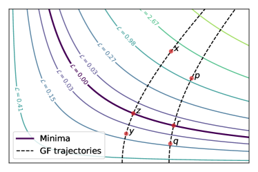
(a)

Figure 1: An illustration of the minima, loss level sets, and trajectories of gradient flow in an example loss landscape. Here $S_{\text{GF}}\left(\boldsymbol{x}\right)=S_{\text{GF}}\left(\boldsymbol{y}\right)=S_{\text{GF}}\left(\boldsymbol{z}\right)=\boldsymbol{z}$ and $S_{\text{GF}}\left(\boldsymbol{p}\right)=S_{\text{GF}}\left(\boldsymbol{q}\right)=S_{\text{GF}}\left(\boldsymbol{r}\right)=\boldsymbol{r}$. Thus, $\phi\left(\boldsymbol{x}\right)=\phi\left(\boldsymbol{y}\right)=\phi\left(\boldsymbol{z}\right)=\lambda_{\max}\left(\nabla^{2}\mathcal{L}\left(\boldsymbol{z}\right)\right)$ and $\phi\left(\boldsymbol{p}\right)=\phi\left(\boldsymbol{q}\right)=\phi\left(\boldsymbol{r}\right)=\lambda_{\max}\left(\nabla^{2}\mathcal{L}\left(\boldsymbol{r}\right)\right)$.

Our main contributions are:

1. For scalar neural networks (i.e., linear networks of unit width and general depth) trained with GD on the quadratic loss, we prove that GD monotonically decreases the GFS sharpness (Theorem 3.2), for a large set of initializations and step sizes (see Figure 2c).

2. Still in the context of scalar networks, we leverage the monotonicity of GFS sharpness as well as a novel quasistatic analysis, and show that if the loss is sufficiently small when the GFS sharpness crosses the stability threshold $\frac{2}{\eta}$, then the final GFS sharpness (and standard sharpness) will be close to $\frac{2}{\eta}$, establishing the EoS phenomenon (Theorem 3.3). This result improves on Zhu et al. (2023) as it holds for a larger class of instances, as we further discuss in Section 2.

3. Finally, we demonstrate empirically that the monotone decrease of the theoretically-derived GFS sharpness extends beyond scalar networks. Specifically, we demonstrate that the monotonic behaviour and convergence to the stability threshold also happens in the squared regression model (Section 4.1) and modern architectures, including fully connected networks with different activation functions, VGG11 with batch-norm, and Resnet20 (Section 4.2).

2 Related Work

The last year saw an intense theoretical study of GD dynamics in the EoS regime. Below, we briefly survey these works, highlighting the aspects that relate to ours.

Analysis under general assumptions.

Several works provide general—albeit sometimes difficult to check—conditions for EoS convergence and related phenomena. Ahn et al. (2022b) relate the non-divergence of GD to the presence of a forward invariant set: we explicitly construct such set for scalar neural networks. Arora et al. (2022); Lyu et al. (2022) relate certain modifications of GD, e.g., normalized GD or GD with weight decay on models with scale invariance, to gradient flow that minimizes the GFS sharpness. In these works, the relation is approximate and valid for sufficiently small step size $\eta$. In contrast, we show exact decrease of the GFS sharpness for fairly finite $\eta$. Ma et al. (2022) relate the non-divergence of unstable GD to sub-quadratic growth of the loss. However, it is not clear whether this is true for neural networks losses; for example, linear neural network with the square loss (including the scalar networks we analyze) are positive polynomials of degree above 2 and hence super-quadratic. Damian et al. (2023) identify a self-stabilization mechanism under which GD converges close to the EoS (similar to the four-stage mechanism identified by Wang et al. (2022b)), under several assumptions. For example, their analysis explicitly assumes progressive sharpening and implicitly assumes a certain “stable set” $\mathcal{M}$ to be well-behaved. While progressive sharpening is easy to test, the existence of a nontrivial $\mathcal{M}$ is less straightforward to verify. In Appendix A, we explain why the set $\mathcal{M}$ is badly-behaved for scalar networks, meaning that the results of Damian et al. (2023) cannot explain the EoS phenomenon for this case.

Analysis of specific objectives.

A second line of works seeks stronger characterizations by examining specific classes of objectives. Chen & Bruna (2022) characterize the periodic behavior of GD with sufficiently large step size in a number of models, including a two layer scalar network. Agarwala et al. (2022) consider squared quadratic functions, and prove that there exist 2-dimensional instances of their model where EoS convergence occur. In order to gain insight into the emergence of threshold neurons, Ahn et al. (2022a) study 2-dimensional objectives of the form $\ell(xy)$ for positive and symmetric loss function $\ell$ satisfying assumptions that exclude the square loss we consider. They provide bounds on the final sharpness of the GD iterates that approach the EoS as $\eta$ decreases. None of these three results have direct implications for the scalar networks we study: Chen & Bruna (2022) are concerned with non-convergent dynamics while Agarwala et al. (2022); Ahn et al. (2022a) consider different models.

Wang et al. (2022a) theoretically studies the balancing effect of large step sizes in a matrix factorization problem of depth 2. They show that the “extent of balancing” decreases, but not necessarily monotonically. Moreover, the model they analyze does not to exhibit the dynamics of the EoS regime (where the sharpness stays slightly above $2/\eta$ for a large number of iterations). Instead, the GFS sharpness and sharpness very quickly decrease below $2/\eta$.

The work most closely related to ours is by Zhu et al. (2023), who study particular 2d slices of 4-layer scalar networks. In our terminology, they re-parameterize the domain into the GFS sharpness and the weight product, and then derive a closed-form approximation for GD’s two-step trajectory, that becomes tight as the step size decreases. Using this approximation they show that, at very small step sizes, GD converges close to the EoS. Furthermore, they interpret the bifuricating and chaotic behavior of GD using a quasistatic approximation of the re-parameterized dynamics.

Compared to Zhu et al. (2023), the key novelty of our analysis is that we identify a simple property (GFS sharpness decrease) that holds for all scalar networks and a large range of step sizes. This property allows us to establish near-EoS convergence without requiring the step size to be very small. Moreover, by considering a more precise quasistatic approximation of GD we obtain a much tighter reconstruction of its bifurcation diagram (see Section B.2) that is furthermore valid for all scalar neural networks.

3 Analysis of Scalar Linear Networks

3.1 Preliminaries

Notation.

We use boldface letters for vectors and matrices. For a vector $\boldsymbol{x}\in\mathbb{R}^{D}$, we denote by $x_{i}$ its $i$-th coordinate, $\pi\left(\boldsymbol{x}\right)\triangleq\prod_{i=1}^{D}x_{i}$ is the product of all the vector coordinates, and $x_{[i]}$ denotes the vector’s $i$-th largest element, i.e., $x_{[1]}\geq x_{[2]}\geq\dots\geq x_{[D]}$. In addition, we denote by $\boldsymbol{x}^{2}$, $\boldsymbol{x}^{-1}$, and $\left|\boldsymbol{x}\right|$ the element-wise square, inverse, and absolute value, respectively. We use $g_{\eta}\left({\boldsymbol{v}}\right)\triangleq\boldsymbol{v}-\eta\nabla\mathcal{L}\left(\boldsymbol{v}\right)$ to the GD update of parameter vector $\boldsymbol{v}$ using step size $\eta$, and we let $\{\boldsymbol{w}^{\left(i\right)}\}_{i\geq 0}$ denote the sequence of GD iterates, i.e., $\boldsymbol{w}^{\left(t+1\right)}\triangleq g_{\eta}\left({\boldsymbol{w}^{\left(t\right)}}\right)$ for every $t\geq 0$. We let $\lambda_{\max}(\boldsymbol{v})$ denote the sharpness at $\boldsymbol{v}$, i.e., the maximal eigenvalue of $\nabla^{2}\mathcal{L}(\boldsymbol{v})$. Finally, we use the standard notation $[N]\triangleq\{1,\dots,N\}$ and $\mathbb{R}_{+}\triangleq\{x\in\mathbb{R}|x>0\}$, and take $\left\|\cdot\right\|$ to be the Euclidean norm throughout.

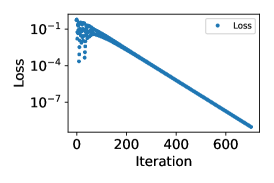
(a)

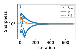
(b)

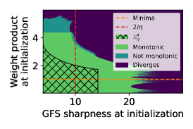
(c)

Figure 2: For a depth 4 scalar network, we apply GD with $\eta=0.2$ for $10^{4}$ steps. In panel LABEL:sub@Fig:_Scalar_network_EoS,_loss the loss exhibits oscillatory behavior while converging to zero. In contrast, in panel LABEL:sub@Fig:_Scalar_network_EoS_sharpness the GFS sharpness is decreasing monotonically until converging to slightly below $\frac{2}{\eta}$; see a zoom-in figure in Figure 8a. In panel LABEL:sub@Fig:_illustration_of_when_the_assumption_is_satisfied, we run GD for different initializations and plot the regions in which the GFS sharpness converges monotonically, non-monotonically, and diverges. We also display the set $\mathbb{S}^{D}_{\eta}$ (see Definition 3.1) from which we prove that GFS sharpness decreases monotonically. We observe that $\mathbb{S}^{D}_{\eta}$ covers a significant portion of the region where GFS sharpness decreases monotonically.

For the theoretical analysis, we consider a scalar linear network with the quadratic loss, i.e., for depth $D\in\mathbb{N}$ and weights $\boldsymbol{w}\in\mathbb{R}^{D}$ the loss function is

$$\mathcal{L}\left(\boldsymbol{w}\right)\triangleq\frac{1}{2}\left(\pi\left(\boldsymbol{w}\right)-1\right)^{2}\,.$$ (1)

This model exhibits EoS behavior, as demonstrated in Figures 2a and 2b, and is perhaps the simplest such model.

Our goal in this section is to prove that (for scalar networks) the GFS sharpness (Definition 1.1) of GD iterates decreases monotonically to a value nor far below the stability threshold $\frac{2}{\eta}$. However, we cannot expect this to hold for all choices of initial weights, since GD diverges for some combinations of step size and initialization. Therefore, to ensure stability for a given step size, we need to make an assumption on the initialization.

To this end, for any weight $\boldsymbol{w}$ we define its GF equivalence class in the interval $I\subseteq\mathbb{R}$ as

$$E_{I}(\boldsymbol{w})\triangleq\left\{\boldsymbol{w^{\prime}}\mid\boldsymbol{w^{\prime}}\overset{\text{GF}}{\sim}\boldsymbol{w}~{}\mbox{and}~{}\pi\left(\boldsymbol{w^{\prime}}\right)\in I\right\}\,,$$ (2)

where $\boldsymbol{w^{\prime}}\overset{\text{GF}}{\sim}\boldsymbol{w}$ if and only if $S_{\text{GF}}\left(\boldsymbol{w^{\prime}}\right)=S_{\text{GF}}\left(\boldsymbol{w}\right)$, e.g., if both vectors lie on the same GF trajectory. Also, for depth $D\geq 2$ and step size $\eta>0$ we define

Definition 3.1 (Positive invariant set).

A weight $\boldsymbol{w}\in\mathbb{R}^{D}$ is in the positive invariant set $\mathbb{S}^{D}_{\eta}$ if and only if there exists $B>1$ such that

1. The coordinate product $\pi(\boldsymbol{w})\in\left(0,B\right)$.

2. For all $\boldsymbol{w}^{\prime}\in E_{\left(0,B\right)}(\boldsymbol{w})$ we have $\pi\left(g_{\eta}\left({\boldsymbol{w}^{\prime}}\right)\right)\in\left(0,B\right)$ (with $E_{\left(0,B\right)}$ defined in Equation 2).

3. The GFS sharpness $\phi\left(\boldsymbol{w}\right)\leq\frac{2\sqrt{2}}{\eta}$.

Roughly, a point $\boldsymbol{w}$ is in $\mathbb{S}^{D}_{\eta}$ if applying a gradient step on weights in the GF trajectory from $\boldsymbol{w}$ does not change its coordinate product $\pi(\boldsymbol{w})$ too much (conditions 1 and 2) and that the GFS sharpness is not large than $\sqrt{2}$ times the stability threshold (condition 3).

In Theorem 3.2 below, we assume that the GD initialization satisfies $\boldsymbol{w}^{(0)}\in\mathbb{S}^{D}_{\eta}$. We note that $\mathbb{S}^{D}_{\eta}$ is non-empty whenever there exists a minimizer with sharpness below $\frac{2}{\eta}$ and empirically appears to be fairly large, as indicated by Figure 2c. We provide additional discussion of the definition of $\mathbb{S}^{D}_{\eta}$ and the parameter $B$ associated with it in Appendix I.

To gain further intuition about the set $\mathbb{S}^{D}_{\eta}$ we define the GFS-preserving GD (GPGD) update step from $\boldsymbol{w}$ to $\boldsymbol{w}^{\prime}$ as:

$$\tilde{g}_{\eta}\left(\boldsymbol{w}\right)\triangleq\boldsymbol{w}^{\prime}\overset{\text{GF}}{\sim}\boldsymbol{w}\text{ such that }\pi\left(\boldsymbol{w}^{\prime}\right)=\pi\left(g_{\eta}\left({\boldsymbol{w}}\right)\right).$$ (3)

That is, in GPGD the next iterate is chosen so that it lies on the GF trajectory from $\boldsymbol{w}$ and its weight product is equal to the weight product of a single gradient step applied to $\boldsymbol{w}$. Note that conditions 1 and 2 in Definition 3.1 can be interpreted as requiring that GPGD initialized at points in $\mathbb{S}^{D}_{\eta}$ does not diverge or change the sign of the product of the weights.

The definition of GPGD is based on the premise that the GFS changes more slowly than the product of the weights, and therefore locally we can approximate GD by keeping the GF projection constant. We discuss GPGD in more detail in Section 3.5, where it plays a key role in the proof of Theorem 3.3.

3.2 Main Results

We can now state our main results.

Theorem 3.2.

Consider GD with step size $\eta>0$ and initialization $\boldsymbol{w}^{(0)}\in\mathbb{S}^{D}_{\eta}$. Then,

1. For all $t\geq 0$, the GD iterates $\boldsymbol{w}^{(t)}$ satisfy $\boldsymbol{w}^{(t)}\in\mathbb{S}^{D}_{\eta}$.

2. The GFS sharpness is monotonic non-inscreasing, i.e., $\phi\left(\boldsymbol{w}^{(t+1)}\right)\leq\phi\left(\boldsymbol{w}^{(t)}\right)$ for all $t\geq 0$.

Theorem 3.2 shows that the set $\mathbb{S}^{D}_{\eta}$ is indeed positive invariant (since GD never leaves it) and moreover that GFS sharpness decreases monotonically for GD iterates in this set.

Figure 2 demonstrates Theorem 3.2. Specifically, in Figure 2b we examine the sharpness and the GFS sharpness when training a scalar neural network with depth $4$. We observe that the GFS sharpness decreases monotonically until reaching $\frac{2}{\eta}$. In addition, Figure 2c illustrates that $\boldsymbol{w}^{(0)}\in\mathbb{S}^{D}_{\eta}$ is indeed sufficient for the GFS sharpness to decrease monotonically and that $\mathbb{S}^{D}_{\eta}$ covers a large portion of the region in GFS sharpness is monotonic. Furthermore, GFS sharpness non-monotonicity tends to occur only in the first few iterations, after which GD enters $\mathbb{S}^{D}_{\eta}$. In Section B.2 (Figure 11) we argue that $\mathbb{S}^{D}_{\eta}$ may even contain regions where GD is chaotic.

While Theorem 3.2 guarantees that GFS sharpness decreases monotonically, we would also like to understand its value at convergence, which equals to the sharpness of the point GD converges to. The next theorem states that once the GFS sharpness reaches below $\frac{2}{\eta}$ (and provided the loss has also decreased sufficiently), then it does not decrease much more and moreover the loss decreases to zero at an exponential rate.

Theorem 3.3.

If for some $t\geq 0$ and $\delta\in(0,0.4]$ we have that $\boldsymbol{w}^{\left(t\right)}\in\mathbb{S}^{D}_{\eta}$, $\phi\left(\boldsymbol{w}^{\left(t\right)}\right)=\frac{2-\delta}{\eta}$ and $\mathcal{L}(\boldsymbol{w}^{\left(t\right)})\leq\delta^{2}/200$ then

1. $\phi\left(\boldsymbol{w}^{\left(t\right)}\right)\geq\frac{2}{\eta}\left(1-\delta\right)$ for all $t\geq 0$.

2. $\mathcal{L}\left(\boldsymbol{w}^{\left(k+t\right)}\right)\leq 2(1-\delta)^{2k}\mathcal{L}\left(\boldsymbol{w}^{\left(t\right)}\right)$ for all $k\geq 1$.

3. The sequence $\{\boldsymbol{w}^{\left(t\right)}\}$ converges.

In Figure 3 we plot the sharpness at GD convergence as a function of initialization, parameterized by initial GFS sharpness and weights product. (Note again that sharpness and GFS sharpness are equal at convergence.) We observe that the sharpness converges to ${2}/{\eta}$ when the GFS sharpness at initialization was larger than ${2}/{\eta}$ and the product of the weights was relatively close to $1$, i.e., the loss was not too large. This demonstrates Theorem 3.3. Additionally, we can see that the condition of the loss being sufficiently small is not only sufficient but also necessary. That is, for initialization with GFS sharpness close to ${2}/{\eta}$ and high loss (i.e., weight product far from 1), the GFS sharpness can converge to values considerably below ${2}/{\eta}$. We also show a specific example in Figure 9.

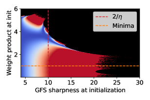
(a)

(b)

Figure 3: Illustration of the sharpness at GD convergence, in the same settings as Figure 2.

3.3 Toward the Proof of Theorem 3.2

To prove the monotonic decrease of GFS sharpness, we identify a quasi-order on scalar linear networks that is monotonic under GD. We call it the “balance” quasi-order and define it below. (Recall that $w_{[i]}$ to denotes the $i$’th largest element in the sequence $w_{1},\ldots,w_{D}$).

Definition 3.4 (Balance quasi-order).

For two scalar networks $\boldsymbol{w},\boldsymbol{v}\in\mathbb{R}^{D}$ we say that $\boldsymbol{w}$ is less unbalanced than $\boldsymbol{v}$, written as $\boldsymbol{w}\leq_{b}\boldsymbol{v}$, if

$$\forall i\in[D-1]:~{}w^{2}_{[i]}-w^{2}_{[i+1]}\leq v^{2}_{[i]}-v^{2}_{[i+1]}\,.$$

Remark 3.5 (Balance invariance under GF).

The ordered balance $b_{i}\left(\boldsymbol{w}\right)\triangleq w^{2}_{[i]}-w^{2}_{[i+1]}$ is invariant under GF, i.e., for any $\boldsymbol{w}^{\prime}\overset{\text{GF}}{\sim}\boldsymbol{w}$ we have $b_{i}\left(\boldsymbol{w}^{\prime}\right)=b_{i}\left(\boldsymbol{w}\right)$ is satisfied for all $i\in[D-1]$ (Arora et al., 2018; Du et al., 2018).

To leverage this quasi-order, we require the related concepts of (log) majorization and a Schur-convex function (Marshall et al., 2011).

Definition 3.6 (Log majorization).

For vectors $\boldsymbol{u},\boldsymbol{v}\in\mathbb{R}_{+}^{D}$ we say that $\boldsymbol{v}$ log majorizes $\boldsymbol{u}$, written as $\boldsymbol{u}\underset{\textup{log}}{\prec}\boldsymbol{v}$, if

$$\prod_{i=1}^{D}u_{\left[i\right]}=\prod_{i=1}^{D}v_{\left[i\right]}~{}\text{and}$$

$$\prod_{i=1}^{k}u_{\left[i\right]}\leq\prod_{i=1}^{k}v_{\left[i\right]}~{}\text{, for every }k\in[D]\,.$$

The balance quasi-order and the log majorization quasi-order are related; we formalize this relation in the following lemma (proof in Appendix F.2).

Lemma 3.7.

For $\boldsymbol{u},\boldsymbol{v}\in\mathbb{R}^{D}$, if $\boldsymbol{u}\leq_{b}\boldsymbol{v}$ and $\prod_{i=1}^{D}u_{i}=\prod_{i=1}^{D}v_{i}$ then $\left|\boldsymbol{u}\right|\underset{\textup{log}}{\prec}\left|\boldsymbol{v}\right|$.

Schur-convex functions are monotonic with respect to majorization, and we analogously define log-Schur convexity.

Definition 3.8 (Log Schur-convexity).

A function $f:\mathcal{A}\mapsto\mathbb{R}$ is log-Schur-convex on $\mathcal{A}\subseteq\mathbb{R}_{+}^{n}$ if for every $\boldsymbol{u},\boldsymbol{v}\in\mathcal{A}$ such that $\boldsymbol{u}\underset{\textup{log}}{\prec}\boldsymbol{v}$ we have $f(\boldsymbol{u})\leq f(\boldsymbol{v})$.

The proof of Theorem 3.2 relies on log-Schur-convexity of the following functions (proof in Appendix F.3).

Lemma 3.9.

The following functions from $\boldsymbol{x}\in\mathbb{R}_{+}^{D}$ to $\mathbb{R}$ are log-Schur-convex:

1. The function $s_{1}\left(\boldsymbol{x}\right)\triangleq\pi^{2}\left(\boldsymbol{x}\right)\left\|\boldsymbol{x}^{-1}\right\|^{2}$ on $\mathbb{R}_{+}^{D}$.

2. The function $-\left[g_{\eta}\left({\boldsymbol{x}}\right)\right]_{\left[D\right]}$ on $\left\{\boldsymbol{x}\in\mathbb{R}_{+}^{D}|\pi\left(\boldsymbol{x}\right)\geq 1\right\}$.

3. The function $\pi\left(g_{\eta}\left({\boldsymbol{x}}\right)\right)$ on $\left\{\boldsymbol{x}\in\mathbb{R}_{+}^{D}|\pi\left(\boldsymbol{x}\right)\leq 1\right\}$.

For a full description of all the definitions, lemmas, and theorems related to majorization and Schur-convexity used in this paper, see Appendix E.

3.4 Proof of Theorem 3.2

We first calculate the Hessian of the loss (1) at an optimum

$$\mathcal{L}\left(\boldsymbol{w}\right)=0\implies\nabla^{2}\mathcal{L}\left(\boldsymbol{w}\right)= \pi^{2}\left(\boldsymbol{w}\right)\boldsymbol{w}^{-1}\left(\boldsymbol{w}^{-1}\right)^{T}\,.$$ (4)

Consequently, if $\boldsymbol{w}^{\star}$ is an optimum, its sharpness is

$$\lambda_{\max}\left(\boldsymbol{w}^{\star}\right) =\pi^{2}\left(\boldsymbol{w}^{\star}\right)\left\|\boldsymbol{w^{\star}}^{-1}\right\|^{2}=s_{1}(\boldsymbol{w}^{\star}),$$ (5)

for the function $s_{1}$ defined in Lemma 3.9.

The proof of Theorem 3.2 relies on the following key lemma that shows that for weights $\boldsymbol{w}\in\mathbb{S}^{D}_{\eta}$ a single step of GD makes the network more balanced (proof in Appendix F.1).

Lemma 3.10.

If $\boldsymbol{w}\in\mathbb{S}^{D}_{\eta}$ then $g_{\eta}\left({\boldsymbol{w}}\right)\leq_{b}\boldsymbol{w}$.

In addition, weights in $\mathbb{S}^{D}_{\eta}$ do not change their sign under GD with step size $\eta$, formally expressed as follows (proof in Section I.1).

Lemma 3.11.

For any $\boldsymbol{w}\in\mathbb{S}^{D}_{\eta}$ and $i\in\left[D\right]$ we have $\operatorname{sign}(\left[g_{\eta}\left({\boldsymbol{w}}\right)\right]_{i})=\operatorname{sign}(\boldsymbol{w}_{i})$.

Combining these results with Lemmas 3.7 and 3.9 we prove Theorem 3.2.

Proof of Theorem 3.2.

We begin by assuming $\boldsymbol{w}^{\left(t\right)}\in\mathbb{S}^{D}_{\eta}$ and showing that $\phi\left(\boldsymbol{w}^{\left(t+1\right)}\right)\leq\phi\left(\boldsymbol{w}^{\left(t\right)}\right)$. To see this, note that $\boldsymbol{w}^{\left(t+1\right)}\leq_{b}\boldsymbol{w}^{\left(t\right)}$ by Lemma 3.10. Since gradient flow preserves the balances, this implies that $S_{\text{GF}}\left(\boldsymbol{w}^{\left(t+1\right)}\right)\leq_{b}S_{\text{GF}}\left(\boldsymbol{w}^{\left(t\right)}\right)$. Moreover, since $\pi\left(S_{\text{GF}}\left(\boldsymbol{w}^{\left(t+1\right)}\right)\right)=\pi\left(S_{\text{GF}}\left(\boldsymbol{w}^{\left(t\right)}\right)\right)=1$, Lemma 3.7 gives $S_{\text{GF}}\left(\boldsymbol{w}^{\left(t+1\right)}\right)\underset{\textup{log}}{\prec}S_{\text{GF}}\left(\boldsymbol{w}^{\left(t\right)}\right)$. Applying Lemma LABEL:*lem:sc functions.1, we get that $s_{1}\left(S_{\text{GF}}\left(\boldsymbol{w}^{\left(t+1\right)}\right)\right)\leq s_{1}\left(S_{\text{GF}}\left(\boldsymbol{w}^{\left(t\right)}\right)\right)$. Recalling Equation 5, we note that $\phi\left(\boldsymbol{v}\right)=s_{1}(S_{\text{GF}}\left(\boldsymbol{v}\right))$ for all $\boldsymbol{v}\in\mathbb{R}^{D}$, completing the proof that $\boldsymbol{w}^{\left(t\right)}\in\mathbb{S}^{D}_{\eta}$ implies $\phi\left(\boldsymbol{w}^{\left(t+1\right)}\right)\leq\phi\left(\boldsymbol{w}^{\left(t\right)}\right)$.

It remains to show that $\boldsymbol{w}^{\left(t\right)}\in\mathbb{S}^{D}_{\eta}$ also implies $\boldsymbol{w}^{\left(t+1\right)}\in\mathbb{S}^{D}_{\eta}$; combined with $\boldsymbol{w}^{\left(0\right)}\in\mathbb{S}^{D}_{\eta}$ this immediately yields $\boldsymbol{w}^{\left(t\right)}\in\mathbb{S}^{D}_{\eta}$ for all $t$ and, via the argument above, monotonicity of $\phi\left(\boldsymbol{w}^{\left(t\right)}\right)$.

Given $\boldsymbol{w}^{\left(t\right)}\in\mathbb{S}^{D}_{\eta}$, we verify that $\boldsymbol{w}^{\left(t+1\right)}\in\mathbb{S}^{D}_{\eta}$ by checking the three conditions in Definition 3.1 of $\mathbb{S}^{D}_{\eta}$. The third condition is already verified, as we have shown that $\phi\left(\boldsymbol{w}^{\left(t+1\right)}\right)\leq\phi\left(\boldsymbol{w}^{\left(t\right)}\right)$, and $\phi\left(\boldsymbol{w}^{\left(t\right)}\right)\leq\frac{2\sqrt{2}}{\eta}$ since $\boldsymbol{w}^{\left(t\right)}\in\mathbb{S}^{D}_{\eta}$. We proceed to verifying the first and second conditions on $\boldsymbol{w}^{\left(t+1\right)}$, assuming they hold on $\boldsymbol{w}^{\left(t\right)}$.

As $\boldsymbol{w}^{\left(t\right)}\in\mathbb{S}^{D}_{\eta}$, there exist $B>1$ such that $\pi\left(\boldsymbol{w}^{\left(t\right)}\right)\in\left(0,B\right)$ and for every $\boldsymbol{u}\in E_{\left(0,B\right)}(\boldsymbol{w}^{\left(t\right)})$ we have $\pi\left(g_{\eta}\left({\boldsymbol{u}}\right)\right)\in\left(0,B\right)$. In particular, we may take $\boldsymbol{u}=\boldsymbol{w}^{\left(t\right)}=E_{\{\pi\left(\boldsymbol{w}^{\left(t\right)}\right)\}}\left(\boldsymbol{w}^{\left(t\right)}\right)$ and conclude that $\pi\left(\boldsymbol{w}^{\left(t+1\right)}\right)=\pi\left(g_{\eta}\left({\boldsymbol{w}^{\left(t\right)}}\right)\right)\in\left(0,B\right)$. Hence, $\boldsymbol{w}^{\left(t+1\right)}$ also satisfies the first condition of Definition 3.1, with the same $B$ as $\boldsymbol{w}^{\left(t\right)}$.

To verify the second condition in Definition 3.1, we fix any $\boldsymbol{v}\in E_{\left(0,B\right)}(\boldsymbol{w}^{\left(t+1\right)})$ and argue that $\pi\left(g_{\eta}\left({\boldsymbol{v}}\right)\right)\in(0,B)$. Using Lemma 3.10 and the fact that balances are invariant under GF, we get that $\boldsymbol{v}\leq_{b}\boldsymbol{u}$, for any $\boldsymbol{u}\in E_{\left(0,B\right)}(\boldsymbol{w}^{\left(t\right)})$. In particular, we take $\boldsymbol{u}^{\prime}\in E_{\{\pi\left(\boldsymbol{v}\right)\}}(\boldsymbol{w}^{\left(t\right)})$ so that $\pi\left(\boldsymbol{v}\right)=\pi\left(\boldsymbol{u}^{\prime}\right)$. Then by using Lemma 3.7 we get that $\boldsymbol{v}\underset{\textup{log}}{\prec}\boldsymbol{u}^{\prime}$. We note that because $\boldsymbol{w}^{\left(t\right)}\in\mathbb{S}^{D}_{\eta}$, $S_{\text{GF}}\left(\boldsymbol{u}^{\prime}\right)=S_{\text{GF}}\left(\boldsymbol{w}^{\left(t\right)}\right)$ and $\pi\left(\boldsymbol{u}^{\prime}\right)\in\left(0,B\right)$ then, from Definition 3.1, we have that $\boldsymbol{u}^{\prime}\in\mathbb{S}^{D}_{\eta}$. Without loss of generality, we assume that $\boldsymbol{v},\boldsymbol{u^{\prime}}\in\mathbb{R}_{+}^{D}$ (see Section D.2.2 for justification).

We now consider two cases:

1. If $\pi\left(\boldsymbol{v}\right)\geq 1$ then, by using Lemma LABEL:*lem:sc functions.2 and the definition of log-Schur-convexity (Definition 3.8), we get that $\left[g_{\eta}\left({\boldsymbol{v}}\right)\right]_{\left[D\right]}\geq\left[g_{\eta}\left({\boldsymbol{u}^{\prime}}\right)\right]_{\left[D\right]}$. In addition, as a consequence of Lemma 3.11 and that $\boldsymbol{u}^{\prime}\in\mathbb{R}_{+}^{D}$, we obtain that $\left[g_{\eta}\left({\boldsymbol{v}}\right)\right]_{\left[D\right]}\geq\left[g_{\eta}\left({\boldsymbol{u}^{\prime}}\right)\right]_{\left[D\right]}>0$. Therefore, $\pi\left(g_{\eta}\left({\boldsymbol{u}^{\prime}}\right)\right)>0$ and also $\pi\left(g_{\eta}\left({\boldsymbol{v}}\right)\right)>0$. Moreover, since $g_{\eta}\left({\boldsymbol{v}}\right)=\boldsymbol{v}-\eta(\pi(\boldsymbol{v})-1)\pi(\boldsymbol{v})\boldsymbol{v}^{-1}$ (see Equation 8 in Section D.1) and $\pi\left(\boldsymbol{v}\right)\geq 1$, we have $g_{\eta}\left({\boldsymbol{v}}\right)\leq\boldsymbol{v}$ elementwise, and therefore (since $g_{\eta}\left({\boldsymbol{v}}\right)\in\mathbb{R}_{+}^{D}$) we have $\pi\left(g_{\eta}\left({\boldsymbol{v}}\right)\right)\leq\pi\left(\boldsymbol{v}\right)<B$. Therefore $\pi\left(g_{\eta}\left({\boldsymbol{v}}\right)\right)\in(0,B)$.

2. If $\pi\left(\boldsymbol{v}\right)\leq 1$ then, by using Lemma LABEL:*lem:sc functions.3, we get that $\pi\left(g_{\eta}\left({\boldsymbol{v}}\right)\right)\leq\pi\left(g_{\eta}\left({\boldsymbol{u}^{\prime}}\right)\right)<B$. Moreover, since $g_{\eta}\left({\boldsymbol{v}}\right)=\boldsymbol{v}-\eta(\pi(\boldsymbol{v})-1)\pi(\boldsymbol{v})\boldsymbol{v}^{-1}$ and $\pi\left(\boldsymbol{v}\right)\leq 1$, we have $g_{\eta}\left({\boldsymbol{v}}\right)\geq\boldsymbol{v}$ elementwise, and therefore (since $\boldsymbol{v}\in\mathbb{R}_{+}^{D}$) we have $0<\pi\left(\boldsymbol{v}\right)\leq\pi\left(g_{\eta}\left({\boldsymbol{v}}\right)\right)$. Therefore $\pi\left(g_{\eta}\left({\boldsymbol{v}}\right)\right)\in(0,B)$.

We conclude that $\pi\left(g_{\eta}\left({\boldsymbol{v}}\right)\right)\in(0,B)$ for all $\boldsymbol{v}\in E_{\left(0,B\right)}(\boldsymbol{w}^{\left(t+1\right)})$, establishing the second condition in Definition 3.1 and completing the proof. ∎

The proof shows that GD monotonically decreases not only the GFS sharpness, but also the balance quasi-order.

3.5 Proof Outline for Theorem 3.3

From Theorem 3.2 we know that the GFS sharpness is decreasing monotonically. Recall that the sharpness and GFS sharpness become identical when GD converges and that GD cannot converge while the sharpness is above $\frac{2}{\eta}$. Thus, unless GD diverges, the GFS sharpness must decrease below $\frac{2}{\eta}$ at some point during the trajectory of GD.

The following lemma lower bounds the change in the GFS sharpness after a single GD step (proof in Appendix G.2).

Lemma 3.12.

For any $t$, if $\boldsymbol{w}^{\left(t\right)}\in\mathbb{S}^{D}_{\eta}$, then

$$\phi\left(\boldsymbol{w}^{\left(t+1\right)}\right)\geq\frac{\phi\left(\boldsymbol{w}^{\left(t\right)}\right)}{1+8\left(\frac{\phi(\boldsymbol{w}^{\left(t\right)})}{2/\eta}\max\{1,\pi(\boldsymbol{w}^{\left(t\right)})\}\right)^{2}\mathcal{L}(\boldsymbol{w}^{\left(t\right)})}.$$

Lemma 3.12 implies that if the loss vanishes sufficiently fast after the GFS sharpness reaches below $\frac{2}{\eta}$, then the GFS sharpness will remain close to $\frac{2}{\eta}$.

Therefore, in order to prove Theorem 3.3 our next goal will be to show that the loss vanishes sufficiently fast. To attain this goal, we use the notion of GPGD defined in Eq. (3). The motivation for using GPGD is that a single step of GD does not change the GFS sharpness too much (Lemma 3.12) and therefore GD and GPGD dynamics are closely related (more on this in Section 3.6). We denote the GPGD update step from $\boldsymbol{w}$ by $\tilde{g}_{\eta}\left(\boldsymbol{w}\right)$.

In the next lemma, we consider a point $\tilde{\boldsymbol{w}}^{\left(0\right)}\in\mathbb{R}^{D}$ with GFS sharpness bounded below the stability threshold, and show GPGD iterates starting from $\tilde{\boldsymbol{w}}^{\left(0\right)}$ converge to zero at an exponential rate (proof in G.3).

Lemma 3.13.

For GPGD iterates $\tilde{\boldsymbol{w}}^{\left(t+1\right)}=\tilde{g}_{\eta}\left(\tilde{\boldsymbol{w}}^{\left(t\right)}\right)$. If $\phi\left(\tilde{\boldsymbol{w}}^{\left(0\right)}\right)=\frac{2-\delta}{\eta}$ for $\delta\in(0,0.5]$ and

$$1-0.1\frac{\delta}{1-\delta}\leq\pi\left(\tilde{\boldsymbol{w}}^{\left(0\right)}\right)\leq 1$$

then for all $t\geq 0$,

$$\mathcal{L}\left(\tilde{\boldsymbol{w}}^{\left(t\right)}\right)\leq\left(1-\delta\right)^{2t}\mathcal{L}\left(\tilde{\boldsymbol{w}}^{\left(0\right)}\right)$$

and the error $\pi\left(\tilde{\boldsymbol{w}}^{\left(t\right)}\right)-1$ changes sign at each iteration.

In the next lemma, we show that the GPGD loss can be used to upper bound the loss of GD (proof in Appendix G.1).

Lemma 3.14.

For any $\boldsymbol{w}\in\mathbb{S}^{D}_{\eta}$, if $\pi\left(\tilde{g}_{\eta}\left(\boldsymbol{w}\right)\right)\geq 1$ and $\phi\left(g_{\eta}\left({\boldsymbol{w}}\right)\right)\geq\frac{1}{\eta}$ then

$$\mathcal{L}\left(g_{\eta}\left({g_{\eta}\left({\boldsymbol{w}}\right)}\right)\right)\leq\mathcal{L}\left(\tilde{g}_{\eta}\left(\tilde{g}_{\eta}\left(\boldsymbol{w}\right)\right)\right)\,,$$

and $\pi\left(g_{\eta}\left({g_{\eta}\left({\boldsymbol{w}}\right)}\right)\right)\leq 1$.

Note that we are interested in comparing the losses after two GD steps (in contrast to a single step) since, from the definition of GPGD, we have that $\mathcal{L}\left(g_{\eta}\left({\boldsymbol{w}}\right)\right)=\mathcal{L}\left(\tilde{g}_{\eta}\left(\boldsymbol{w}\right)\right)$.

Overall, combining Lemma 3.13 and Lemma 3.14 we prove that GD loss vanishes exponentially fast and combining this result with Lemma 3.12 we obtain the lower bound on GFS sharpness, given in Theorem 3.3 (see Appendix H for the full proof).

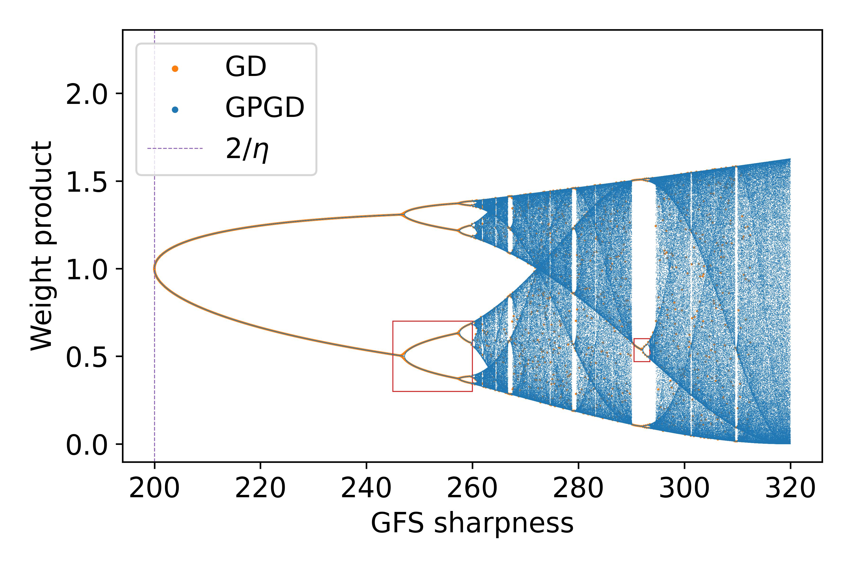
Figure 4: GD follows the GPGD bifurcation diagram. See Figure 10 for additional description and zoomed-in plots.

3.6 GD Follows the GPGD Bifurcation Diagram

Lemma 3.13 implies that, when the GFS sharpness is below $\frac{2}{\eta}$, GPGD converges to the global minimum of the loss. In contrast, if the GFS sharpness is above $\frac{2}{\eta}$ then either GPGD behaves chaotically or it converges to a periodic sequence.

In 4 we summarize the behavior of GPGD with a bifurcation diagram, showing the weight product of its periodic points as a function of GFS sharpness (which is constant for each GPGD trajectory). The figure also shows the values of $(\phi(\boldsymbol{w}^{\left(t\right)}),\pi(\boldsymbol{w}^{\left(t\right)}))$ for a GD trajectory—demonstrating that they very nearly coincide with the GPGD periodic points.

The observation that GD follows the GPGD bifurcation diagram gives us another perspective on the convergence to the edge of stability and on the non-monotonic convergence of the loss to zero: when GD is initialized with GFS sharpness above the stability threshold, it “enables” GPGD to converge to loss zero by slowly decreasing the GFS sharpness until reaching the stability threshold $\frac{2}{\eta}$. Since GD closely approximates the GPGD periodic points throughout, it follows that when reaching GFS sharpness close to $\frac{2}{\eta}$, GD must be very close to the period 1 point of GPGD, which is exactly the minimizer of the loss $\mathcal{L}$ with sharpness $\frac{2}{\eta}$.

In Section B.2 we provide more details on the GPGD bifurcation diagram, as well as zoomed-in plots and a comparison with the bifurcation diagram obtained by the approximate dynamics of Zhu et al. (2023).

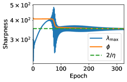
(a)

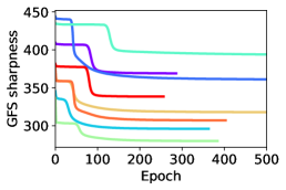
(b)

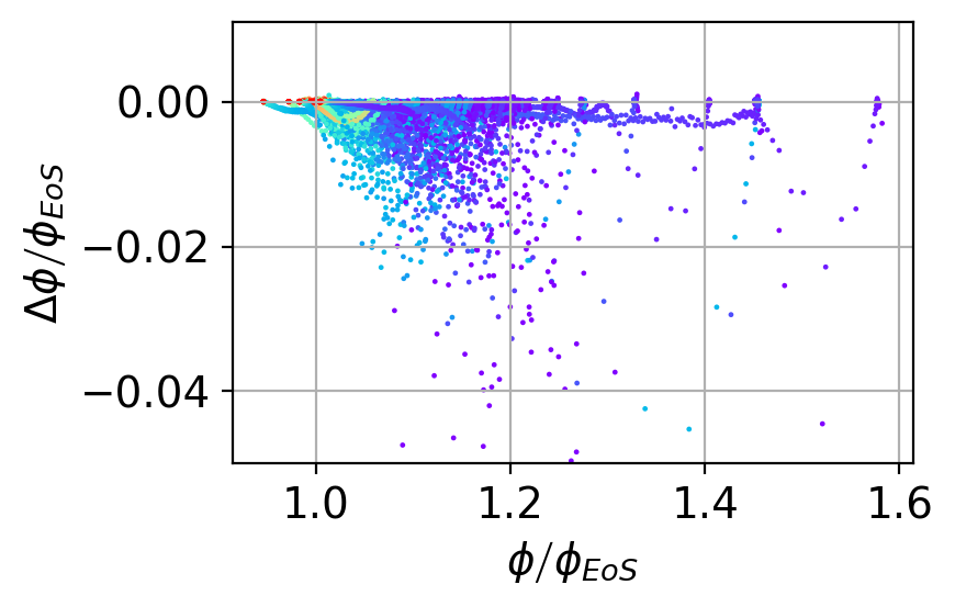
(c)

Figure 5: The GFS sharpness exhibits consistent monotonic decrease for the squared regression model. For MSE loss and the squared regression model with random synthetic data, we apply GD until the training loss decreases below $0.01$. We calculate the GFS sharpness at each iteration using Eq. (7). We repeat this experiment with $50$ different seeds (i.e., 50 different random datasets and initializations) and two large learning rates per seed: $\eta_{1}=0.85\cdot\frac{2}{\min_{\boldsymbol{\theta}}\lambda_{\max}\left(\boldsymbol{\theta}\right)},\,\eta_{2}=0.99\cdot\frac{2}{\min_{\boldsymbol{\theta}}\lambda_{\max}\left(\boldsymbol{\theta}\right)}$. Note that the sharpness of the flattest implementation $\min_{\boldsymbol{\theta}}\lambda_{\max}\left(\boldsymbol{\theta}\right)$ varies for each random dataset. Full implementation details are given in Appendix B.3. In all three figures, we observe that GFS sharpness decreases monotonically for various seeds and step sizes. See detailed discussion in Section 4.1.

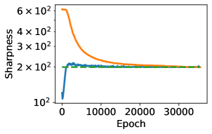
(a) FC-hardtanh

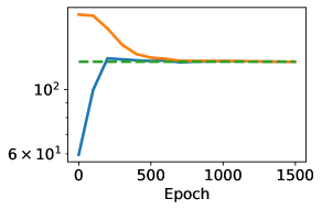
(b) VGG11-bn

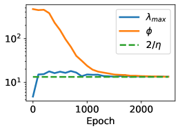
(c) ResNet20

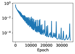
(d) FC-hardtanh

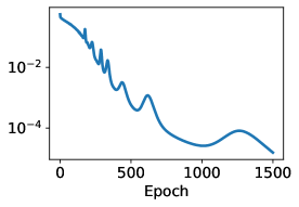
(e) VGG11-bn

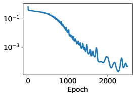
(f) ResNet20

Figure 6: The GFS sharpness decrease monotonically to $2/\eta$ for common neural network architectures. On three architectures, we run GD on a subset of CIFAR10 and calculate the GFS sharpness every 100 iterations using the Runge-Kutta algorithm. The sharpness (blue line) non-monotonically rises to the EoS $2/\eta$ (green dashed line) and the GFS sharpness (orange line) decreases monotonically to the same value. In contrast, at the bottom figures, we observe that the training loss exhibits non-monotonic and chaotic behavior.

4 Experiments

Our goal in this and the following section is to test whether monotonic decrease of GFS sharpness holds beyond scalar linear networks. In Section 4.1 consider a simple model where we can compute GFS sharpness exactly, while in Section 4.2 we approximate GFS sharpness for practical neural networks. Overall, we find empirically that GD monotonically decreases GFS sharpness well beyond scalar networks.

4.1 Squared Regression Model

We consider the squared regression model

$$f_{\boldsymbol{\theta}}\left(\boldsymbol{x}\right)=\left\langle\boldsymbol{u}_{+}^{2}-\boldsymbol{u}_{-}^{2},\boldsymbol{x}\right\rangle=\left\langle\boldsymbol{\beta},\boldsymbol{x}\right\rangle\,.$$ (6)

This 2-positive homogeneous model is analyzed in several previous works (e.g., Woodworth et al., 2020; Gissin et al., 2020; Moroshko et al., 2020; Pesme et al., 2021; Azulay et al., 2021). Importantly, for the MSE loss, Azulay et al. (2021) show that the linear predictor associated with the interpolating solution obtained by GF initialized at some $\boldsymbol{w}_{0}=\begin{bmatrix}\boldsymbol{u}_{+,0}^{\top}&\boldsymbol{u}_{-,0}^{\top}\end{bmatrix}^{\top}\in\mathbb{R}^{2d}$ where $\boldsymbol{w}_{0}\neq\boldsymbol{0}$ (element-wise) can be obtained by solving the following problem:

$$\boldsymbol{\beta}_{GF}\left(\boldsymbol{w}_{0}\right)=\operatorname*{argmin}_{\boldsymbol{\beta}}Q_{\boldsymbol{w}_{0}}\left(\boldsymbol{\beta}\right)\text{ s.t. }\boldsymbol{X\beta}=\boldsymbol{y}\,,$$ (7)

where $\boldsymbol{X}$ and $\boldsymbol{y}$ are the training data and labels respectively,

$$Q_{\boldsymbol{w}_{0}}\left(\boldsymbol{\beta}\right)= \sum_{i=1}^{d}\left|w_{0,i}w_{0,i+d}\right|q\left(\frac{\beta_{i}}{2\left|w_{0,i}w_{0,i+d}\right|}\right)$$

$$-\frac{1}{2}\boldsymbol{\beta}^{\top}\operatorname{arcsinh}\left(\frac{w_{0,i}^{2}-w_{0,i+d}^{2}}{2\left|w_{0,i}w_{0,i+d}\right|}\right)\,,$$

and

$$q\left(z\right)=1-\sqrt{1+z^{2}}+z\operatorname{arcsinh}\left(z\right)\,.$$

Using this result, we can calculate the GFS sharpness efficiently in this model. (Full details in Appendix C.)

In Figure 5, we summarize the results of running GD on synthetic random data until the training loss decreased below $0.01$ and calculating the GFS sharpness at each iteration using Eq. (7). We repeat this experiment with $50$ different seeds and two large learning rates per seed.

Qualitative behavior of GFS sharpness.

In Figure 5a we examine the sharpness ($\lambda_{\max}$, blue line), GFS sharpness ($\phi$, orange line) and the stability threshold ($2/\eta$, green line) for a single experiment. We observe that the GFS sharpness remains constant until the sharpness crosses the stability threshold $2/\eta$. This is expected since GD tracks the GF trajectory when the sharpness is much smaller than the stability threshold. Then, once the sharpness increased beyond $2/\eta$, we observe the GFS sharpness decreasing monotonically until converging at approximately $2/\eta$. In Figure 5b we examine the GFS sharpness obtained in eight different experiments and observe the same qualitative behavior.

Quantitative behavior of GFS sharpness.

In Figure 5c, to examine the consistency of the GFS sharpness monotonic behavior, we calculate for $100$ experiments the normalized change in the GFS sharpness, i.e.,

$$\frac{\Delta\phi}{\phi_{EoS}}(t)=\frac{\phi\left(\boldsymbol{w}\left(t+1\right)\right)-\phi\left(\boldsymbol{w}\left(t\right)\right)}{2/\eta},$$

and produce a scatter plot of all $70,539$ points of the form $(\frac{\phi(\boldsymbol{w}^{\left(t\right)})}{\phi_{\mathrm{EoS}}},\frac{\Delta\phi}{\phi_{EoS}}(t))$, colored by $t$. We observe that the normalized difference change in the GFS sharpness is always below $0.00104$, with roughly $78\%$ of the points being negative. That is, the GFS sharpness consistently exhibits decreasing monotonic behavior, with the few small positive values occurring early in the optimization.

4.2 Realistic Neural Networks

We now consider common neural network architectures. For such networks, there is no simple expression for the GF solution when initialized at some $\boldsymbol{w}_{0}$. Therefore, we used Runge-Kutta RK4 algorithm (Press et al., 2007) to numerically approximate the GF trajectory, similarly to (Cohen et al., 2021).

In Figure 6, we plot the sharpness, GFS sharpness, and training loss on three different architectures: three layers fully connected (FC) network with hardtanh activation function (the same architecture used in (Cohen et al., 2021)), VGG11 with batch normalization (BN), and ResNet20 with BN. The fully connected network and the VGG11 networks were trained on a $1$K example subset of CIFAR10, and the ResNet was trained on a $100$ example subset of CIFAR10. We only used a subset of CIFAR10 for our experiments since each experiment required many calculations of the GFS sharpness by running Runge-Kutta algorithm until the training loss is sufficiently small (we use a convergence threshold of $10^{-5}$) which is computationally difficult. Full implementation details are given in Appendix B.4.

In the figure, we observe that GFS sharpness monotonicity also occurs in modern neural networks. Similar to the scalar network and the squared regression model, we observe that the GFS sharpness decreases until reaching the stability threshold $2/\eta$. In contrast, we observe that the training loss oscillates while decreasing over long time scales.

In Figures 12 and 13 in Appendix B.5, we observe the same qualitative behavior on more architectures (FC with tanh and ReLU activations) and another dataset (SVHN). We note that we occasionally see a slight increase in GFS sharpness early in the optimization (see Figures 6c and 12b).

5 Discussion

In this work, for scalar linear networks, we show that GD monotonically decreases the GFS sharpness. In addition, we use the fact that GD tracks closely the GPGD dynamics to show that if the loss is sufficiently small when the GFS sharpness decreases below the stability threshold $\frac{2}{\eta}$, then the GFS sharpness will stay close to the $\frac{2}{\eta}$ and the loss will converge to zero. This provides a new perspective on the mechanism behind the EoS behaviour. Finally, we demonstrate empirically that GFS sharpness monotonicity extends beyond scalar networks. A natural future direction is extending our analysis beyond scalar linear networks.

There are several additional directions for future work. First, it will be interesting to explore how the GFS sharpness (or some generalization thereof) behaves for other loss functions. Note that this extension is not trivial since for losses with an exponential tail, e.g., cross-entropy, the Hessian vanishes as the loss goes to zero. Therefore, on separable data, the GFS sharpness vanishes. A second direction is the stochastic setting. Namely, it will be interesting to understand whether stochastic gradient descent and Adam also exhibit some kind of GFS sharpness monotonicity, as the EoS phenomenon has been observed for these methods as well (Lee & Jang (2023) and Cohen et al. (2022)).

Finally, a third direction is studying GFS sharpness for non-constant step sizes, considering common practices such as learning rate schedules or warmup. We generally expect GFS sharpness to remain monotonic even for non-constant step sizes. More specifically, for scalar neural networks and GD with schedule $\eta_{t}$, the GFS sharpness will be monotone when $\boldsymbol{w}^{(t)}\in\mathbb{S}_{\eta_{t}}^{D}$ for all $t$. In particular, since the set $\mathbb{S}_{\eta}^{D}$ increases as $\eta$ decreases (see Lemma I.1), i.e., $\mathbb{S}_{\eta_{t_{1}}}^{D}\subseteq\mathbb{S}_{\eta_{t_{2}}}^{D}$ for any $\eta_{t_{1}}\geq\eta_{t_{2}}$, we get that for a scalar network with $\boldsymbol{w}^{(0)}\in\mathbb{S}_{\eta_{0}}^{D}$, the GFS sharpness will decrease monotonically for any decreasing step size schedule. In addition, it may be possible to view warmup (i.e., starting from a small step size and then increasing it gradually) as a technique for ensuring that $\boldsymbol{w}^{\left(t\right)}\in\mathbb{S}_{\eta_{t}}^{D}$ for all $t$ and a larger set of initializations $\boldsymbol{w}^{\left(0\right)}$, giving a complementary perspective to prior work such as Gilmer et al. (2022).

Appendix A Discussion of Damian et al. (2023) in the Setting of Scalar Networks

Damian et al. (2023) study the EoS phenomenon and introduce a “self-stabilization” theory. In this section, we explain why this analysis cannot adequately explain the EoS phenomenon in scalar networks.

The analysis of Damian et al. (2023) relies on the notation of the “stable set”

$$\mathcal{M}\triangleq\left\{\boldsymbol{w}~{}~{}:~{}~{}\lambda_{\max}\left(\nabla^{2}\mathcal{L}\left(\boldsymbol{w}\right)\right)\leq 2/\eta~{}\text{and}~{}\nabla\mathcal{L}\left(\boldsymbol{w}\right)\cdot u\left(\boldsymbol{w}\right)=0\right\},$$

where $\mathcal{L}$ is the loss and $u(\boldsymbol{w})$ is the top eigenvector of the loss Hessian (assumed to be unique). They argue that, under certain assumptions, GD tracks the constrained trajectory of GD projected to $\mathcal{M}$.

However, for scalar networks with square loss, we observe that $\mathcal{M}$ consists of two disjoint sets: all stable global minima (points with zero loss), and another set of points with strictly positive loss. Theoretically, we can see this from the expressions for the loss gradient and Hessians (equations (8) and (11), respectively). When the loss is small we have:

$$\nabla\mathcal{L}\left(\boldsymbol{w}\right)\cdot u\left(\boldsymbol{w}\right)\approx\left(\pi(\boldsymbol{w})-1\right)\pi(\boldsymbol{w})\left\|\boldsymbol{w}^{-1}\right\|$$

which is non-zero when the loss is non-zero. Empirically, in Figure 7, we numerically compute $\nabla\mathcal{L}\left(\boldsymbol{w}\right)\cdot u\left(\boldsymbol{w}\right)$ for depth 3 scalar networks, and observe that the set $\mathcal{M}$ is contained in

$$\left\{\boldsymbol{w}:\mathcal{L}\left(\boldsymbol{w}\right)=0\right\}\cup\left\{\boldsymbol{w}~{}~{}:~{}~{}w_{[2]}=w_{[3]}~{}\text{and}~{}w_{1}w_{2}w_{3}=\frac{1}{2}\right\},$$

Confirming that the set of minima is a disjoint component in $\mathcal{M}$.

Therefore, for scalar networks the projected GD considered by Damian et al. (2023) cannot smoothly decrease the loss toward zero. This contradicts their theoretical results (e.g., their Lemma 8) meaning that their assumptions do not hold for scalar networks.

Finally, we also note that Equations (9) and (10) in our paper imply that, if $w_{[D-1]}=w_{[D]}$ and the product of the weights $\pi\left(\boldsymbol{w}\right)$ is $\frac{1}{2}$, then the Hessian is a diagonal matrix where the top eigenvalue is not unique. This contradicts an assumption made on the top eigenvalue function $u$ (Damian et al., 2023, Definition 1).

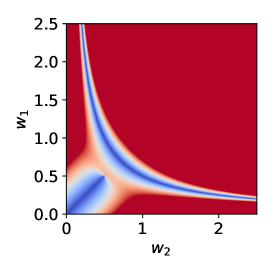
(a) $w_{3}=2.0$

(b) $w_{3}=1.5$

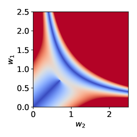
(c) $w_{3}=1.0$

(d) $w_{3}=0.9$

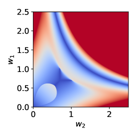
(e) $w_{3}=0.7$

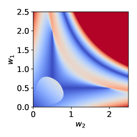
(f) $w_{3}=0.5$

(g)

Figure 7: Illustration of the values of $\left|\nabla\mathcal{L}\left(\boldsymbol{w}\right)\cdot u\left(\boldsymbol{w}\right)\right|$ for different weights for scalar networks of depth $3$. We observe that the condition $\nabla\mathcal{L}\left(\boldsymbol{w}\right)\cdot u\left(\boldsymbol{w}\right)=0$ implies that $\boldsymbol{w}\in\left\{\boldsymbol{w}:\mathcal{L}\left(\boldsymbol{w}\right)=0\right\}\cup\left\{\boldsymbol{w}~{}~{}:~{}~{}w_{[2]}=w_{[3]}~{}\text{and}~{}w_{1}w_{2}w_{3}=\frac{1}{2}\right\}.$

Appendix B Additional Experiments and Implementation Details

B.1 Sharpness at Convergence for Scalar Networks

Note that it is not possible to converge to a minimum with sharpness larger than $\frac{2}{\eta}$ (e.g., Ahn et al., 2022b). In Theorem 3.3 we show that, under certain conditions, scalar network converge to a minimum with sharpness that is only slightly smaller than $\frac{2}{\eta}$. In Figure 8, we show a zoomed-in version of Figure 2b to illustrate that indeed the scalar network converged to sharpness slightly below $\frac{2}{\eta}$.

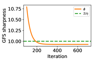
(a)

Figure 8: The GFS sharpness converges to slightly below $\frac{2}{\eta}$. This is a zoomed-in version of Figure 2b.

In Figure 9, we run GD in the same setting as in Figure 2, i.e. step size of $0.2$ and a scalar network of depth 4. The specific initialization of $[2.57213954,2.57213954,0.65589001,0.65589001]$ was chosen by examining Figure 3 and selecting an initialization with GFS sharpness above $\frac{2}{\eta}$ but converging to sharpness that is relatively far below $\frac{2}{\eta}$. In the figure we can see an example in which the loss was fairly large (loss of 5.1) when the GFS sharpness crossed $\frac{2}{\eta}$, thus not satisfying the condition in Theorem 3.3 and converging to a sharpness value relatively far below $\frac{2}{\eta}$.

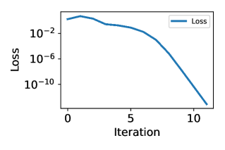
(a)

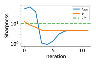
(b)

Figure 9: The GFS sharpness can converge significantly below $\frac{2}{\eta}$. The figure shows a depth 4 network with initialization $[2.57213954,2.57213954,0.65589001,0.65589001]$ and GD step size $0.2$.We observe that GFS sharpness converges relatively far below $\frac{2}{\eta}$.

B.2 GD Follows the GPGD Bifurcation Diagram

This section supplements Section 3.6, providing additional details on the GFS-preserving GD (GPGD) bifurcation diagram, a comparison with (Zhu et al., 2023), and evidence that the set $\mathbb{S}^{D}_{\eta}$ may contain point where GD exhibits chaotic behavior.

Computation of GPGD bifurication diagram.

To compute the GPGD bifurcation diagram, we first compute the GD trajectory $\boldsymbol{w}^{\left(t\right)}$. For each $t$, we run $K=5\cdot 10^{6}$ steps of GPGD as defined in Equation 3, starting from $\boldsymbol{w}^{\left(t\right)}$, resulting in the sequence $\tilde{\boldsymbol{w}}^{(t,1)},\ldots,\tilde{\boldsymbol{w}}^{(t,K)}$. We then add all the points of the form $\{(\phi(\boldsymbol{w}^{\left(t\right)}),\pi(\tilde{\boldsymbol{w}}^{(t,K-k)}))\}_{t\geq 0,k\in[0,10^{4})}$ to the scatter plot forming the GPGD bifurcation diagram (note that $\phi(\tilde{\boldsymbol{w}}^{(t,k)})=\phi(\boldsymbol{w}^{\left(t\right)})$ for all $t$ and $k$ by definition of GPGD). That is, we let GPGD converge to a limiting period (when it exists), and then plot the last few iterates.

Comparison with Zhu et al. (2023).

Zhu et al. (2023) analyze scalar networks of depth 4, initialized so that $w_{1}=w_{2}$ and $w_{3}=w_{4}$ for all points in the GD trajectory. They approximate the (two-step) dynamics of the GFS sharpness $\phi(\boldsymbol{w}^{\left(t\right)})$ and the weight product $\pi(\boldsymbol{w}^{\left(t\right)})$ assuming that $\eta$ is small, and observe that the $\phi(\boldsymbol{w}^{\left(t\right)})$ updates are of a lower order in $\eta$. Consequently, they consider an approximation wherein the GFS sharpness is fixed to some value $\phi$, and the weight product evolves according to a scalar recursion parameterized by $\phi$. Similar to GPGD, for different values of $\phi$ the approximated $\pi$ dynamics either converge to a periodic solution or becomes chaotic. Figure 10a shows this bifurcation diagram of the approximate dynamics superimposed on values of $(\phi(\boldsymbol{w}^{\left(t\right)}),\pi(\boldsymbol{w}^{\left(t\right)}))$ of the true GD trajectory, reproducing Figure 6c from (Zhu et al., 2023). The figure shows that the bifurcation diagram is qualitatively similar to the GD trajectory, but does not approximate it well. By contrast, GPGD provides a close approximation of the GD dynamics for a wide of range GFS sharpness values.

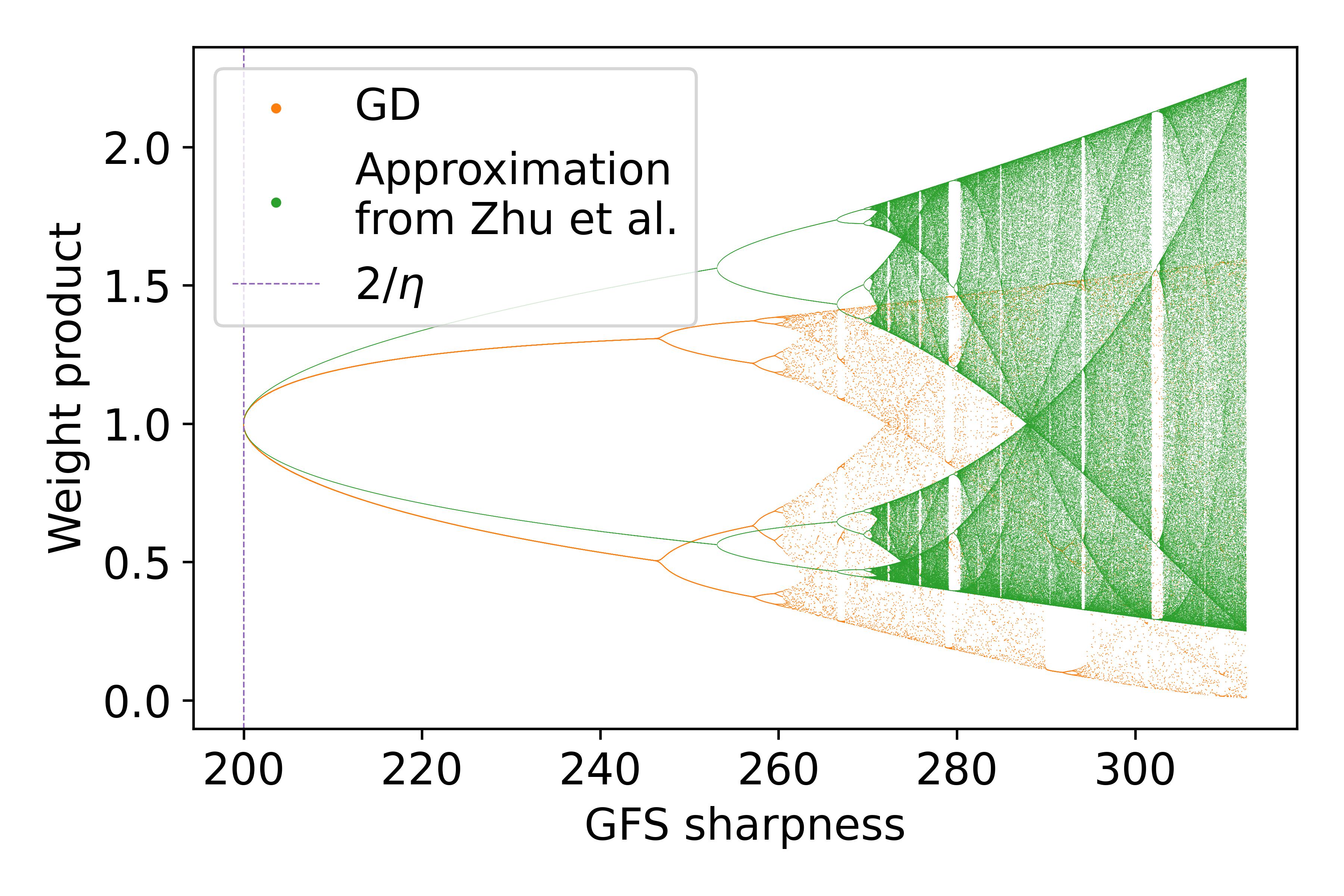
(a) GD iterates compared to approximation from Zhu et al. (2023)

(b) GD iterates compared to GPGD

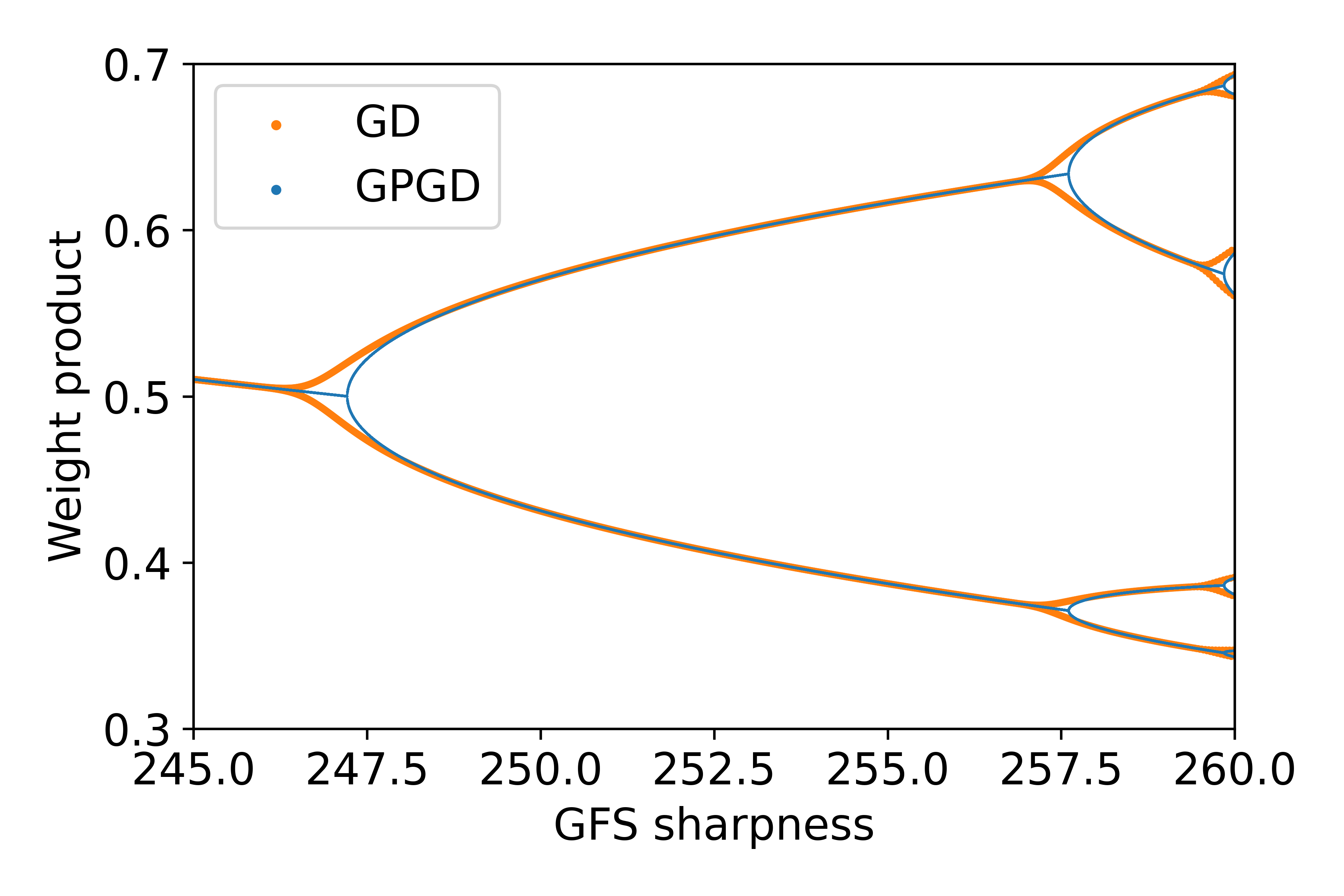
(c) Zoom in (left)

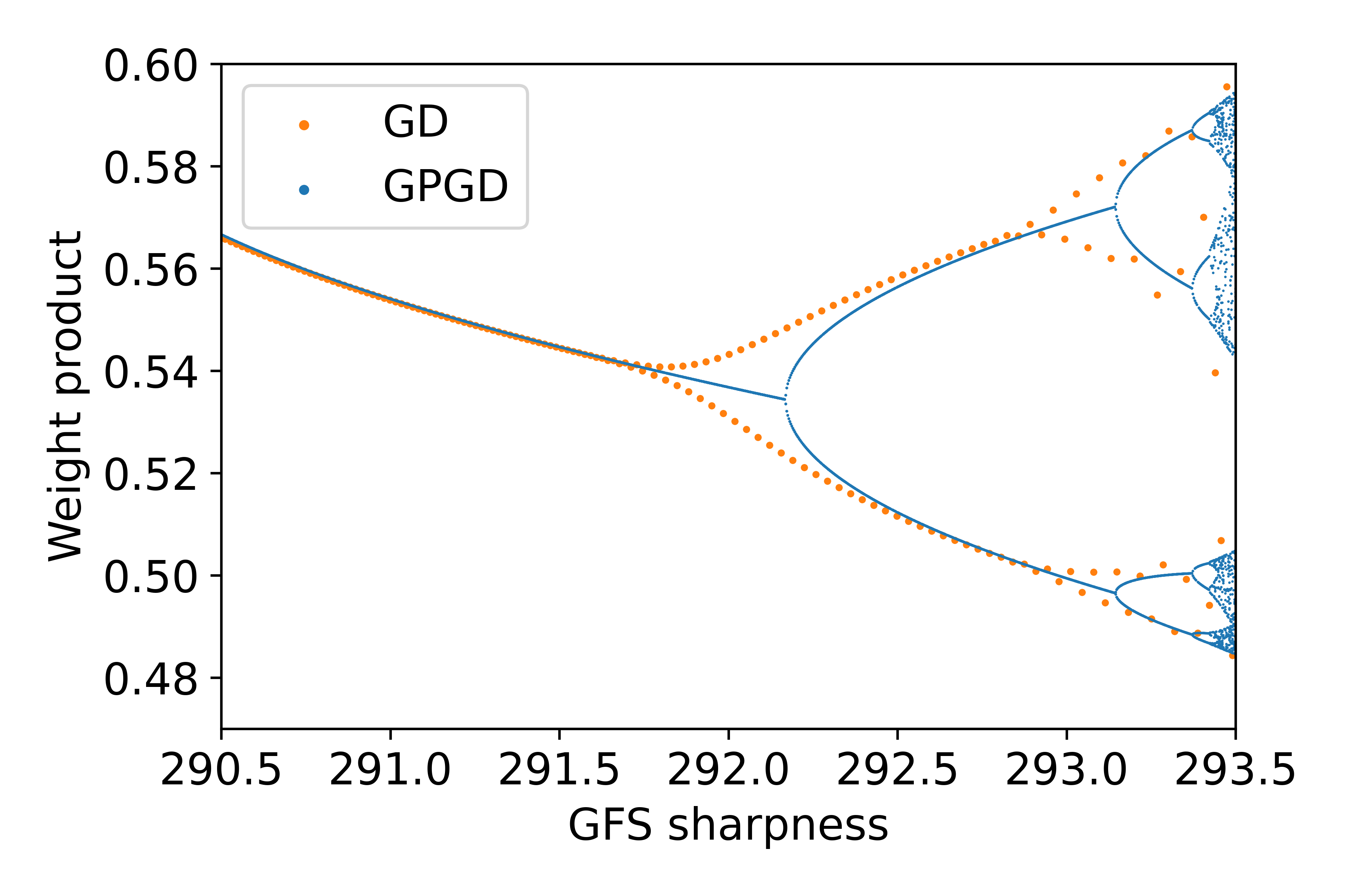
(d) Zoom in (right)

Figure 10: GD tracks the GPGD bifurcation diagram. For a scalar linear network with depth $4$, initialization of $[12.5,12.5,0.05,0.05]$, and $\eta=\frac{2}{200}=0.01$. LABEL:sub@Fig:bifurcation_GD_vs_B The bifurcation diagram of the approximate dynamics proposed by Zhu et al. (2023) is qualitatively similar to the GD trajectory, but does not approximate it well. LABEL:sub@Fig:bifurcation_GD_vs_GPGD The GPGD bifurcation diagram approximates the GD trajectory very closely. When the GFS sharpness is close to $\frac{2}{\eta}=200$ both GP and GPGD attain loss $0$ (y axis value $1$), meaning we converge close to the stability threshold. LABEL:sub@Fig:bifurcation_zoom_in_left and LABEL:sub@Fig:bifurcation_zoom_in_right Zoom-in on regions highlighted in panel LABEL:sub@Fig:bifurcation_GD_vs_B, showing the GPGD bifurcation diagram and GPGD diverge slightly near bifurcation points.

$\mathbb{S}^{D}_{\eta}$ contains points where GD is chaotic.

The similarity between GD and GPGD allows up to identify the chaotic parts of the GD trajectory with the chaotic states of GPGD. More precisely we say that GD is chaotic at iterate $\boldsymbol{w}^{\left(t\right)}$ if starting iterating GPGD starting from $\boldsymbol{w}^{\left(t\right)}$ does not converge to a periodic sequence. Figure 11 demonstrate that the set $\mathbb{S}^{D}_{\eta}$ in which the GFS sharpness is guaranteed to decrease can contain such chaotic points. By contrast, the approximation of Zhu et al. (2023) is only valid when the approximate dynamics are periodic with period 2 or less.

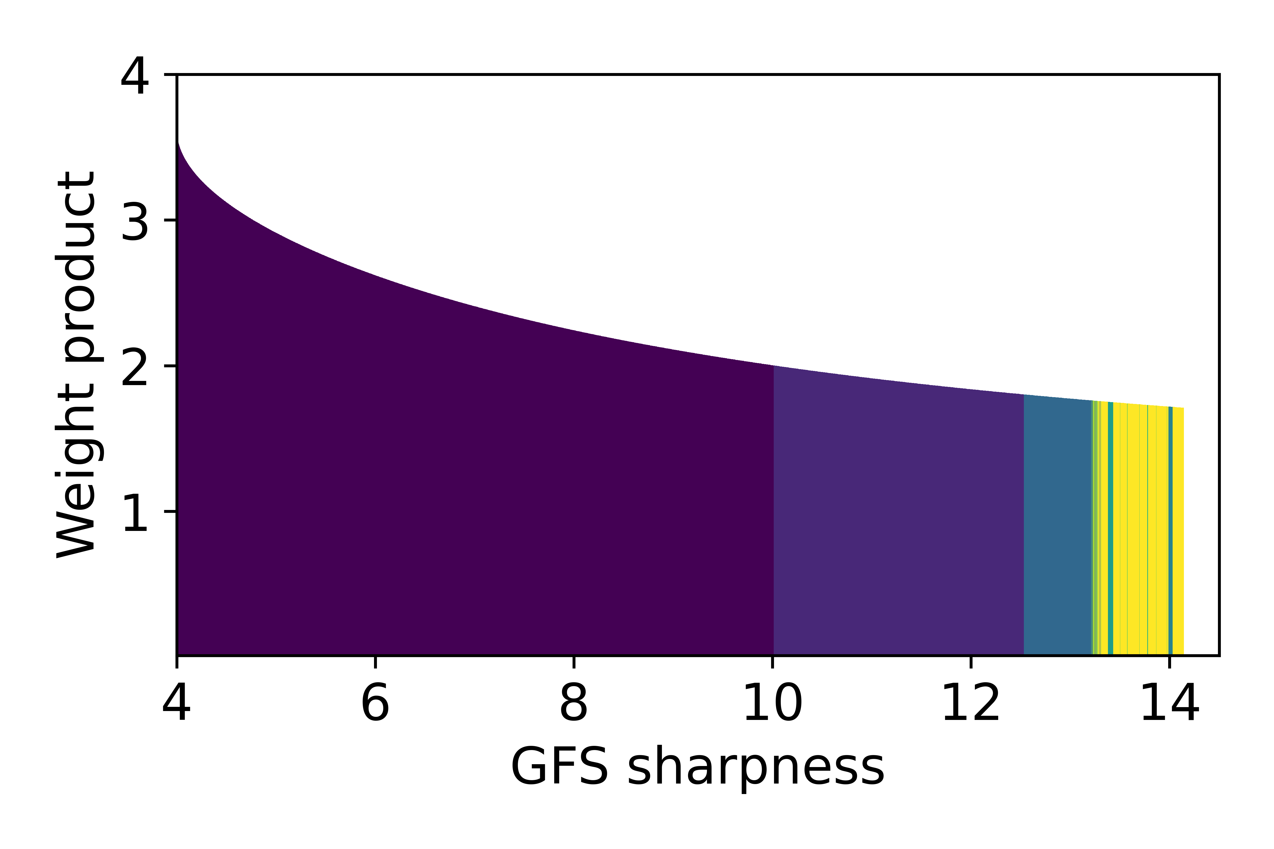
(a)

(b)

Figure 11: $\mathbb{S}^{D}_{\eta}$ contains points where GD is chaotic. For every point in $\mathbb{S}^{D}_{\eta}$ the figure presents the period of the bifurcation diagram of the GPGD for the same GFS sharpness. We observe that $\mathbb{S}^{D}_{\eta}$ contains points with a large range of periods going from 1 (convergence) to above 512 (indicating chaotic behavior). The figure is generated with the same settings as Figure 2c and Figure 3.

B.3 Implementation Details for the Squared Regression Experiments (Figure 5)

To examine the GFS sharpness behavior for the squared regression model we run GD on a synthetic Gaussian i.i.d. dataset $\left(\boldsymbol{x}_{n},y_{n}\right)_{n=1}^{N}$ where $\boldsymbol{x}_{n}\sim\mathcal{N}\left(\boldsymbol{\mu},\boldsymbol{\Sigma}\right)$ with $\boldsymbol{\mu}=5\cdot\boldsymbol{1}_{d}$, $\Sigma=5\cdot\boldsymbol{I}_{d\times d}$, $d=100$ and $N=50$. Here, $\boldsymbol{1}_{d}\in\mathbb{R}^{d}$ is a vector containing all ones and $\boldsymbol{I}_{d\times d}\in\mathbb{R}^{s\times s}$ is the identity matrix. Our stopping criterion was the loss decreasing below a threshold of $0.01$. At each iteration, we calculated the GFS sharpness using Eq. (7) and the the SciPy optimization package. We repeat this experiment with $50$ different seeds and two large learning rates per seed: $\eta_{1}=0.85\cdot(2/\min_{\boldsymbol{\theta}}\lambda_{\max}\left(\boldsymbol{\theta}\right))$ and $\eta_{2}=0.99\cdot(2/\min_{\boldsymbol{\theta}}\lambda_{\max}\left(\boldsymbol{\theta}\right))$ per seed. Note that $\min_{\boldsymbol{\theta}}\lambda_{\max}\left(\boldsymbol{\theta}\right)$, i.e., the sharpness of the flattest implementation, varies for each random dataset, i.e., for each seed. To obtain the sharpness of the flattest implementation we use projected GD with Dykstra’s projection algorithm.

B.4 Implementation Details for Realistic Neural Networks (Figure 6)

Generally, we followed a similar setting to Cohen et al. (2021), with some necessary adjustments due to the computational cost of calculating the GFS sharpness repeatedly.

Dataset. The dataset consists of the first $1000$ samples from CIFAR-10, except for the ResNet experiment in which the dataset consists of a subset of the $100$ first samples. We used the same preprocessing as Cohen et al. (2021). That is, we centered each channel, and then normalized the channel by dividing it by the standard deviation (where both the mean and standard deviation were computed over the full CIFAR-10 dataset).

Architectures. We experiment with five architectures: three layers fully connected networks with hardtanh, tanh, and ReLU activation function (the same architecture as in Cohen et al. (2021)), VGG-11 with batch normalization (implemented here: https://github.com/chengyangfu/pytorch-vgg-cifar10/blob/master/vgg.py), and ResNet20 (implemented here: https://github.com/hongyi-zhang/Fixup).

Loss. The MSE loss was used in the experiments.

GFS sharpness computation. We calculated the GFS sharpness every $100$ iterations since it was too computationally expensive to do this calculation at each iteration, as in the squared regression model experiments. In order to calculate the GFS sharpness at a given iteration of GD, we used the Runge-Kutta RK4 algorithm (Press et al., 2007) to numerically approximate the GF trajectory initialized at the current iterate of GD. In other words, given GD iterate at time $t$: $\boldsymbol{w}^{\left(t\right)}$, we used Runge-Kutta until reaching training loss below $10^{-5}$ to compute $S_{\text{GF}}\left(\boldsymbol{w}^{\left(t\right)}\right)$. Then, we calculated the maximal eigenvalue of $S_{\text{GF}}\left(\boldsymbol{w}^{\left(t\right)}\right)$ using Lanczos algorithm to obtain the GFS sharpness. Similar to Cohen et al. (2021) we used $1/\lambda_{\max}(\boldsymbol{w}^{\left(t\right)})$ as the step size for Runge-Kutta algorithm.

B.5 Additional Experiments on Realistic Architectures

In Figure 12, we experiment in the same setting as in Figure 6 for two additional activation functions. We observe the same qualitative behavior as in Figure 6.

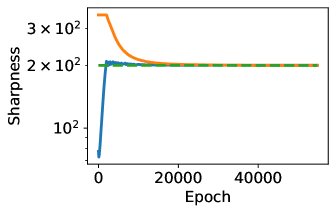
(a) FC-tanh

(b) FC-ReLU

(c)

Figure 12: The GFS sharpness decrease monotonically to $2/\eta$ for common neural network architectures. On two additional architectures, we run GD on a subset of Cifar10 and calculated the GFS sharpness every 100 iterations using Runge-Kutta algorithm. We observe the same qualitative behavior as in Figure 6: the sharpness (blue line) non-monotonically rises to the EoS, i.e., to $2/\eta$ (green dashed line) and the GFS sharpness (orange line) decrease monotonically to the same value.

In Figure 13 we repeat the experiments on a subset of $1000$ samples from the SVHN dataset. Again, we observe the same qualitative behavior as in Figure 6.

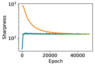
(a) FC-ReLU-svhn

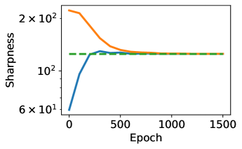
(b) vgg11-bn-svhn

(c)

Figure 13: The GFS sharpness decreases monotonically to $2/\eta$ for common neural network architectures on an additional dataset. Using a subset of the SVHN dataset, we run GD and calculated the GFS sharpness every 100 iterations using Runge-Kutta algorithm. We observe the same qualitative behavior as in Figure 6: the sharpness (blue line) non-monotonically rises to the EoS, i.e., to $2/\eta$ (green dashed line) and the GFS sharpness (orange line) decrease monotonically to the same value.

Appendix C Calculation of the GFS and its Sharpness for the Squared Regression Model

Setting.

Given a training set $\left\{\boldsymbol{x}_{n},y_{n}\right\}_{n=1}^{N}$, we define the square loss

$$\mathcal{L}\left(\boldsymbol{\theta}\right)=\frac{1}{2N}\sum_{n=1}^{N}\left(y_{n}-f_{\boldsymbol{\theta}}\left(\boldsymbol{x}_{n}\right)\right)^{2}$$

where $f_{\boldsymbol{\theta}}\left(\boldsymbol{x}\right)=\left\langle\boldsymbol{u}_{+}^{2}-\boldsymbol{u}_{-}^{2},\boldsymbol{x}\right\rangle=\left\langle\boldsymbol{\beta},\boldsymbol{x}\right\rangle.$

In this section, we explain how we obtain the GFS sharpness for this setting, i.e., the squared regression model. There are three main steps:

1. Obtaining the optimization problem for finding $\boldsymbol{\beta}_{GF}\left(\boldsymbol{w}_{0}\right)$ (the linear predictor associated with the interpolating solution obtained by GF initialized at $\boldsymbol{w}_{0}$) using the result from (Azulay et al., 2021) Appendix A.

2. Obtaining $S_{\text{GF}}\left(\boldsymbol{w}_{0}\right)^{2}$ from $\boldsymbol{\beta}_{GF}\left(\boldsymbol{w}_{0}\right)$.

3. Obtaining the GFS sharpness.

Obtaining the optimization problem for finding $\boldsymbol{\beta}_{GF}\left(\boldsymbol{w}_{0}\right)$.

Following the calculations in (Azulay et al., 2021) Appendix A, and substituting $\boldsymbol{v}_{+}=\boldsymbol{u}_{+}$ and $\boldsymbol{v}_{-}=\boldsymbol{u}_{-}$, we obtain that

$$\boldsymbol{\beta}_{GF}\left(\boldsymbol{w}_{0}\right)=\operatorname*{argmin}_{\boldsymbol{\beta}}Q_{\boldsymbol{w}_{0}}\left(\boldsymbol{\beta}\right)\text{ s.t. }\boldsymbol{X\beta}=\boldsymbol{y}\,,$$

where $\boldsymbol{X}$ and $\boldsymbol{y}$ are the training data and labels respectively,

$$Q_{\boldsymbol{w}_{0}}\left(\boldsymbol{\beta}\right)= \sum_{i=1}^{d}q_{k_{i}}\left(\beta_{i}\right)\,,$$

for $k_{i}=16w_{0,i}^{2}w_{0,i+d}^{2}$ and

$$q^{\prime\prime}_{k_{i}}\left(\beta_{i}\right)=\frac{1}{\sqrt{k_{i}+4\beta_{i}^{2}}}\,.$$

Integrating the above, and using the constraint $q^{\prime}_{k_{i}}\left(\beta_{0,i}\right)=0$ where $\beta_{0,i}=w_{0,i}^{2}-w_{0,i+d}^{2}$ we get:

$$q_{k_{i}}^{\prime}\left(\beta_{i}\right)= \frac{1}{4}\left[\log\left(\frac{2\beta_{i}}{\sqrt{k_{i}+4\beta_{i}^{2}}}+1\right)-\log\left(1-\frac{2\beta_{i}}{\sqrt{k_{i}+4\beta_{i}^{2}}}\right)\right]$$

$$-\frac{1}{4}\left[\log\left(\frac{2\beta_{0,i}}{\sqrt{k_{i}+4\beta_{0,i}^{2}}}+1\right)-\log\left(1-\frac{2\beta_{0,i}}{\sqrt{k_{i}+4\beta_{0,i}^{2}}}\right)\right]$$

Simplifying the above we obtain:

$$q_{k_{i}}^{\prime}\left(\beta_{i}\right) =\frac{1}{4}\left[\log\left(\frac{2\beta_{i}+\sqrt{k_{i}+4\beta_{i}^{2}}}{\sqrt{k_{i}+4\beta_{i}^{2}}-2\beta_{i}}\right)-\log\left(\frac{2\beta_{0,i}+\sqrt{k_{i}+4\beta_{0,i}^{2}}}{\sqrt{k_{i}+4\beta_{0,i}^{2}}-2\beta_{0,i}}\right)\right]$$

$$=\frac{1}{2}\left[\log\left(2\beta_{i}+\sqrt{k_{i}+4\beta_{i}^{2}}\right)-\log\left(2\beta_{0,i}+\sqrt{k_{i}+4\beta_{0,i}^{2}}\right)\right]$$

$$=\frac{1}{2}\left[\log\left(\frac{2\beta_{i}}{\sqrt{k_{i}}}+\sqrt{1+\frac{4\beta_{i}^{2}}{k_{i}}}\right)-\log\left(\frac{2\beta_{0,i}}{\sqrt{k_{i}}}+\sqrt{1+\frac{4\beta_{0,i}^{2}}{k_{i}}}\right)\right]$$

$$=\frac{1}{2}\left[\operatorname{arcsinh}\left(\frac{2\beta_{i}}{\sqrt{k_{i}}}\right)-\operatorname{arcsinh}\left(\frac{2\beta_{0,i}}{\sqrt{k_{i}}}\right)\right]$$

Finally, we integrate again and obtain

$$q_{k_{i}}\left(\beta_{i}\right) =\int q_{k_{i}}^{\prime}\left(\beta_{i}\right)=\frac{\sqrt{k_{i}}}{4}\left[1-\sqrt{1+\frac{4\beta_{i}^{2}}{k_{i}}}+\frac{2\beta_{i}}{\sqrt{k_{i}}}\operatorname{arcsinh}\left(\frac{2\beta_{i}}{\sqrt{k_{i}}}\right)\right]-\frac{1}{2}\operatorname{arcsinh}\left(\frac{2\beta_{0,i}}{\sqrt{k_{i}}}\right)\beta_{i}\,.$$

Substituting $k_{i}=16w_{0,i}^{2}w_{0,i+d}^{2}$ and $\beta_{0,i}=w_{0,i}^{2}-w_{0,i+d}^{2}$ we obtain the desired result, i.e.,

$$Q_{\boldsymbol{w}_{0}}\left(\boldsymbol{\beta}\right)= \sum_{i=1}^{d}\left|w_{0,i}w_{0,i+d}\right|q\left(\frac{\beta_{i}}{2\left|w_{0,i}w_{0,i+d}\right|}\right)$$

$$-\frac{1}{2}\boldsymbol{\beta}^{\top}\operatorname{arcsinh}\left(\frac{w_{0,i}^{2}-w_{0,i+d}^{2}}{2\left|w_{0,i}w_{0,i+d}\right|}\right)\,,$$

where

$$q\left(z\right)=1-\sqrt{1+z^{2}}+z\operatorname{arcsinh}\left(z\right)\,.$$

Obtaining $S_{\text{GF}}\left(\boldsymbol{w}_{0}\right)^{2}$ from $\boldsymbol{\beta}_{GF}\left(\boldsymbol{w}_{0}\right)$.

Using the squared regression model definition and Eq. $(17)$ in (Azulay et al., 2021) (the preserved quantity for this model) we obtain

$$\begin{cases}u_{+,i}u_{-,i}=u_{+,0,i}u_{-,0,i}\\ \beta_{i}=u_{+,i}^{2}-u_{-,i}^{2}\,,\end{cases}$$

where, from definition, $u_{+,0,i}=w_{0,i}\,,u_{-,0,i}=w_{0,i+d}$. From these two equations, we get

$$u_{+,i}^{2}\left(\beta_{i}\right) =\frac{\beta_{i}+\sqrt{\beta_{i}^{2}+4u_{+,0,i}^{2}u_{-,0,i}^{2}}}{2}$$

$$u_{-,i}^{2}\left(\beta_{i}\right) =\frac{-\beta_{i}+\sqrt{\beta_{i}^{2}+4u_{+,0,i}^{2}u_{-,0,i}^{2}}}{2}$$

This immediately gives us $S_{\text{GF}}\left(\boldsymbol{w}_{0}\right)^{2}$ since from definition $S_{\text{GF}}\left(\boldsymbol{w}_{0}\right)^{2}=\begin{bmatrix}\boldsymbol{u}_{+}^{2}\left(\beta_{GF}\right)&\boldsymbol{u}_{-}^{2}\left(\beta_{GF}\right)\end{bmatrix}$.

Obtaining the GFS sharpness.

We denote $\boldsymbol{\theta}=\begin{bmatrix}\boldsymbol{u}_{+}^{\top}&\boldsymbol{u}_{-}^{\top}\end{bmatrix}^{\top}$. The Hessian matrix for the squared regression model is

$$\nabla^{2}\mathcal{L}\left(\boldsymbol{\theta}\right)=\frac{1}{N}\sum_{n=1}^{N}\nabla_{\boldsymbol{\theta}}f_{\boldsymbol{\theta}}\left(\boldsymbol{x}_{n}\right)\nabla_{\boldsymbol{\theta}}f_{\boldsymbol{\theta}}\left(\boldsymbol{x}_{n}\right)^{\top}+\frac{1}{N}\sum_{n=1}^{N}\left(f_{\boldsymbol{\theta}}\left(\boldsymbol{x}_{n}\right)-y_{n}\right)\nabla_{\boldsymbol{\theta}}^{2}f_{\boldsymbol{\theta}}\left(\boldsymbol{x}_{n}\right)\,,$$

where

$$\nabla_{\boldsymbol{\theta}}f_{\boldsymbol{\theta}}\left(\boldsymbol{x}_{n}\right) =2\boldsymbol{\theta}\circ\begin{bmatrix}\boldsymbol{x}_{n}\\ -\boldsymbol{x}_{n}\end{bmatrix}\,,$$

$$\nabla_{\boldsymbol{\theta}}^{2}f_{\boldsymbol{\theta}}\left(\boldsymbol{x}_{n}\right) =2\mathrm{diag}\left(\begin{bmatrix}\boldsymbol{x}_{n}\\ -\boldsymbol{x}_{n}\end{bmatrix}\right)$$

and $\circ$ denotes element-wise multiplication. Thus, to obtain the GFS sharpness all we need to do is substitute $\boldsymbol{\theta}=\left|S_{\text{GF}}\left(\boldsymbol{w}_{0}\right)\right|$ and calculate the maximal eigenvalue. (Note that the sign of the elements of $S_{\text{GF}}\left(\boldsymbol{w}_{0}\right)$ does not affect the maximal eigenvalue.)

Appendix D Properties of GD in Scalar Networks

D.1 Gradient and Hessian Calculation

The partial derivative of the loss defined in Equation 1 is

$$\frac{\partial\mathcal{L}\left(\boldsymbol{w}\right)}{\partial w_{i}} =\left(\pi\left(\boldsymbol{w}\right)-1\right)\frac{\partial\pi\left(\boldsymbol{w}\right)}{\partial w_{i}}$$

$$=\left(\pi\left(\boldsymbol{w}\right)-1\right)\prod_{k\in[D]-\{i\}}w_{k}$$

$$=\left(\pi\left(\boldsymbol{w}\right)-1\right)\frac{\pi\left(\boldsymbol{w}\right)}{w_{i}}\,.$$

Therefore, the gradient is

$$\nabla\mathcal{L}\left(\boldsymbol{w}\right)=\left(\pi\left(\boldsymbol{w}\right)-1\right)\pi\left(\boldsymbol{w}\right)\boldsymbol{w}^{-1}\,.$$ (8)

The second order partial derivative, if $i\neq j$, is

$$\frac{\partial^{2}\mathcal{L}\left(\boldsymbol{w}\right)}{\partial w_{i}\partial w_{j}} =\frac{\pi^{2}\left(\boldsymbol{w}\right)}{w_{i}w_{j}}+\left(\pi\left(\boldsymbol{w}\right)-1\right)\frac{\pi\left(\boldsymbol{w}\right)}{w_{i}w_{j}}\,,$$ (9)

and if $i=j$, it is

$$\frac{\partial^{2}\mathcal{L}\left(\boldsymbol{w}\right)}{\partial w_{i}^{2}} =\frac{\pi^{2}\left(\boldsymbol{w}\right)}{w_{i}^{2}}\,.$$ (10)

Therefore, if weight $\boldsymbol{w}$ is an optimum, i.e. $\pi\left(\boldsymbol{w}\right)=1$ then the Hessian is

$$\nabla^{2}\mathcal{L}\left(\boldsymbol{w}\right) =\pi^{2}\left(\boldsymbol{w}\right)\boldsymbol{w}^{-1}\left(\boldsymbol{w}^{-1}\right)^{T}\,.$$ (11)

Thus, if weight $\boldsymbol{w}$ is an optimum, the largest eigenvalue of the Hessian is

$$\lambda_{\max} =\pi^{2}\left(\boldsymbol{w}\right)\left(\boldsymbol{w}^{-1}\right)^{T}\boldsymbol{w}^{-1}$$ (12)

$$=s_{1}(\boldsymbol{w})\,.$$

D.2 The Dynamics of GD

The exact update rule of gradient decent with a fixed step size $\eta\in\mathbb{R}_{+}$ on the loss function described in Equation 1, using the gradient in Equation 8, is

$$w^{(t+1)}_{i}=w^{(t)}_{i}-\eta\left(\prod_{j=1}^{D}w^{(t)}_{j}-1\right)\prod_{j\in[D]-\{i\}}w^{(t)}_{j}\,,$$ (13)

We can separate the gradient decent dynamics into two separate dynamics, a dynamic of the weights product and a dynamic of the balances.

To this end, for every $m\in\left[D\right]\cup\left\{0\right\}$, define

$$s_{m}(\boldsymbol{w})=\sum_{\begin{subarray}{c}I=\text{ subset of }\\ D-m\text{ different}\\ \text{indices from }[D]\end{subarray}}\prod_{i\in I}{w_{i}^{2}}\,.$$

The dynamics of the product of the weight is

$$\pi^{(t+1)} =\pi^{(t)}+\sum_{m=1}^{D}\eta^{m}(1-\pi^{(t)})^{m}{\pi^{(t)}}^{m-1}s_{m}(\boldsymbol{w}^{(t)})\,,$$ (14)

where $\pi^{(t)}=\pi(w^{(t)})$, see Section D.2.1 for full calculation.

We define the balances as

Definition D.1 (Balances).

The balances $\boldsymbol{b}\in\mathbb{R}^{D\times D}$, of weight $\boldsymbol{w}$, are define as

$$b_{i,j}\triangleq{w_{i}}^{2}-{w_{j}}^{2}\,,~{}\forall i,j\in\left[D\right]\,.$$

The dynamics of the balances, for each $i,j\in[D],i\neq j$, is

$$b_{i,j}^{\left(t+1\right)} =b_{i,j}^{\left(t\right)}\left(1-\eta^{2}\left(\pi^{(t)}-1\right)^{2}\frac{{\pi^{(t)}}^{2}}{{w^{(t)}_{i}}^{2}{w^{(t)}_{j}}^{2}}\right)\,,$$ (15)

where $b_{i,j}^{\left(t\right)}$ are the balances of $\boldsymbol{w}^{\left(t\right)}$, see Section D.2.1 for full calculation. Note that while $\frac{{\pi^{(t)}}^{2}}{{w^{(t)}_{i}}^{2}{w^{(t)}_{j}}^{2}}$ is not define if either $w^{(t)}_{i}$ or $w^{(t)}_{j}$ are equal to $0$, the limit of $\frac{{\pi^{(t)}}^{2}}{{w^{(t)}_{i}}^{2}{w^{(t)}_{j}}^{2}}$ when either of $w^{(t)}_{i}$ or $w^{(t)}_{j}$ approaches $0$ does exist and equal to $\prod_{k\in[D]-\{i,j\}}{w^{(t)}_{k}}^{2}$.

The balances and the product of the weight are sufficient to find the value of ${\boldsymbol{w}^{(t)}}^{2}$, which is needed for calculating the update step in both of the dynamics. Therefore, we can indirectly calculate Equation 13 using Equation 14 and Equation 15.

D.2.1 Dynamics calculation

The dynamic of the product of the weight, written in Equation 14, is found by

$$\pi^{(t+1)} =\prod_{i=1}^{D}w^{(t+1)}_{i}$$

$$=\prod_{i=1}^{D}\left(w^{(t)}_{i}-\eta\left(\pi^{(t)}-1\right)\frac{\pi^{(t)}}{w^{(t)}_{i}}\right)$$

$$=\pi^{(t)}\prod_{i=1}^{D}\left(1-\eta\left(\pi^{(t)}-1\right)\frac{\pi^{(t)}}{{w^{(t)}_{i}}^{2}}\right)$$

$$=\pi^{(t)}+\sum_{m=1}^{D}\eta^{m}(1-\pi^{(t)})^{m}{\pi^{(t)}}^{m-1}s_{m}(\boldsymbol{w}^{(t)})\,.$$

The dynamic of the balances, written in Equation 15, is found by

$$b_{i,j}^{\left(t+1\right)} ={w^{\left(t+1\right)}_{i}}^{2}-{w^{\left(t+1\right)}_{j}}^{2}$$

$$=\left(w^{(t)}_{i}-\eta\left(\pi^{(t)}-1\right)\frac{\pi^{(t)}}{w^{(t)}_{i}}\right)^{2}-\left(w^{(t)}_{j}-\eta\left(\pi^{(t)}-1\right)\frac{\pi^{(t)}}{w^{(t)}_{j}}\right)^{2}$$

$$={w^{\left(t\right)}_{i}}^{2}-2\eta\left(\pi^{(t)}-1\right)\pi^{(t)}+\eta^{2}\left(\pi^{(t)}-1\right)^{2}\frac{{\pi^{(t)}}^{2}}{{w^{\left(t\right)}_{i}}^{2}}$$

$$\qquad-{w^{\left(t\right)}_{j}}^{2}+2\eta\left(\pi^{(t)}-1\right)\pi^{(t)}-\eta^{2}\left(\pi^{(t)}-1\right)^{2}\frac{{\pi^{(t)}}^{2}}{{w^{\left(t\right)}_{j}}^{2}}$$

$$={w^{\left(t\right)}_{i}}^{2}-{w^{\left(t\right)}_{j}}^{2}+\eta^{2}\left(\pi^{(t)}-1\right)^{2}{\pi^{(t)}}^{2}\left(\frac{1}{{w^{\left(t\right)}_{i}}^{2}}-\frac{1}{{w^{\left(t\right)}_{j}}^{2}}\right)$$

$$=\left({w^{\left(t\right)}_{i}}^{2}-{w^{\left(t\right)}_{j}}^{2}\right)\left(1-\eta^{2}\left(\pi^{(t)}-1\right)^{2}\frac{{\pi^{(t)}}^{2}}{{w^{(t)}_{i}}^{2}{w^{(t)}_{j}}^{2}}\right)$$

$$=b_{i,j}^{\left(t\right)}\left(1-\eta^{2}\left(\pi^{(t)}-1\right)^{2}\frac{{\pi^{(t)}}^{2}}{{w^{(t)}_{i}}^{2}{w^{(t)}_{j}}^{2}}\right)\,.$$

D.2.2 Equivalence of weights

Note that in order to calculate the dynamics of the weights (Equation 14)) and balances (Equation 15), we do not need to know the individual sign of every element of $\boldsymbol{w}$. Instead, only the sign of $\pi\left(w\right)$ and the values of the elements of $\boldsymbol{w}^{2}$ are needed to calculate the dynamics. Therefore, if $\pi\left(w\right)\geq 0$, then $\boldsymbol{w}$ will have the same GD dynamics as $\left|\boldsymbol{w}\right|$.

In addition, if $\boldsymbol{w}$ is a minimum then $\left|\boldsymbol{w}\right|$ is also a minimum, and Equation 5 implies it has the shame sharpness.

Appendix E Majorization and Schur-Convexity

Definitions, lemmas and theorems are taken from (Marshall et al., 2011).

We first define Schur-convexity.

Definition E.1 (Majorization).

For vectors $\boldsymbol{u},\boldsymbol{v}\in\mathbb{R}^{n}$ we say that $\boldsymbol{v}$ majorizes $\boldsymbol{u}$, written as $\boldsymbol{u}\prec\boldsymbol{v}$, if

$$\sum_{i=1}^{D}u_{\left[i\right]}=\sum_{i=1}^{D}v_{\left[i\right]}~{}\text{and}$$

$$\sum_{i=1}^{k}u_{\left[i\right]}\leq\sum_{i=1}^{k}v_{\left[i\right]}~{}\text{, for every }k\in[D]\,.$$

Definition E.2 (Schur-convexity).

A function $f:\mathbb{R}^{n}\mapsto\mathbb{R}$ is called Schur-convex if for every vectors $\boldsymbol{u},\boldsymbol{v}\in\mathbb{R}^{n}$ such that $\boldsymbol{u}\prec\boldsymbol{v}$, then $f(\boldsymbol{u})\leq f(\boldsymbol{v})$.

A symmetric function is defined as

Definition E.3 (Symmetric function).

A function $f:\mathbb{R}^{n}\mapsto\mathbb{R}$ is symmetric if for every vector $\boldsymbol{u}\in\mathbb{R}^{n}$ and for every permutation $\boldsymbol{u}^{\prime}$ of vector $\boldsymbol{u}$ then $f\left(\boldsymbol{u}^{\prime}\right)=f\left(\boldsymbol{u}\right)$.

In our derivation, we will use the following useful theorems regarding Schur-convex functions.

Theorem E.4.

If a function $f:\mathbb{R}^{n}\mapsto\mathbb{R}$ is symmetric and convex, then $f$ is Schur-convex.

Theorem E.5.

Let $\mathcal{A}\subseteq\mathbb{R}^{n}$ be a set with the property

$$\boldsymbol{v}\in\mathcal{A}\text{,}\,\boldsymbol{u}\in\mathbb{R}^{n}~{}\text{and}~{}\boldsymbol{u}\prec\boldsymbol{v}\qquad\text{implies}\quad\boldsymbol{u}\in\mathcal{A}\,.$$

A continuous function $f:\mathcal{A}\mapsto\mathbb{R}$ is Schur-convex if $f$ is symmetric and for every vector $\boldsymbol{v}\in\mathcal{A}$ and for every $k\in\left[n-1\right]$ then

$$f\left(\boldsymbol{v}_{\left[1\right]},\dots,\boldsymbol{v}_{\left[k-1\right]},\boldsymbol{v}_{\left[k\right]}+\varepsilon,\boldsymbol{v}_{\left[k+1\right]}-\varepsilon,\boldsymbol{v}_{\left[k+2\right]},\dots,\boldsymbol{v}_{\left[n\right]}\right)$$

is raising in $\varepsilon$ over the region

$$0\leq\varepsilon\leq\min\left\{\boldsymbol{v}_{\left[k-1\right]}-\boldsymbol{v}_{\left[k\right]},\boldsymbol{v}_{\left[k+1\right]}-\boldsymbol{v}_{\left[k+2\right]}\right\}\,,$$

where $\boldsymbol{v}_{\left[0\right]}\triangleq\infty$ and $\boldsymbol{v}_{\left[n+1\right]}\triangleq-\infty$.

Finally, we present a lemma that can be used to apply the previous theorems to what we called log-Schur-convex functions (Definition 3.8).

Lemma E.6.

Let $\mathcal{A}\subseteq\mathbb{R}_{+}^{n}$. For a function $f:\mathcal{A}\mapsto\mathbb{R}$ if $f\left(e^{\boldsymbol{x}}\right)$ is Schur-convex on $\log\mathcal{A}$, where $e^{\boldsymbol{x}}$ is preformed element-wise and $\log\mathcal{A}$ is preformed element-wise on each element of $\mathcal{A}$, then for every vectors $\boldsymbol{u},\boldsymbol{v}\in\mathbb{R}_{+}^{n}$ such that $\boldsymbol{u}\underset{\textup{log}}{\prec}\boldsymbol{v}$ we have that $f(\boldsymbol{u})\leq f(\boldsymbol{v})$, i.e., $f$ is log-Schur-convex.

Note that the term log-Schur-convex function is not often used in literature. Instead, Lemma E.6 is used together with Schur-convex functions. However, for convenience, in our derivation, we decided to define and use log-Schur-convexity directly.

Appendix F Proof of Lemmas 3.10, 3.7, and 3.9

F.1 Proof of Lemma 3.10

The proof of Lemma 3.10 relies on two auxiliary lemmas:

Lemma F.1.

For $D\geq 2$, $\eta>0$ and $\boldsymbol{w}\in\mathbb{R}^{D}$, if $\phi\left(\boldsymbol{w}\right)\leq\frac{2\sqrt{2}}{\eta}$ and $\pi\left(\boldsymbol{w}\right)\in\left[0,1\right]$ then

$$\sum_{i=1}^{\min\{2,D-1\}}\frac{\eta^{2}\left(\pi(\boldsymbol{w})-1\right)^{2}\pi^{2}(\boldsymbol{w})}{w^{2}_{[D-i]}w^{2}_{[D]}}\leq 2\,.$$

Lemma F.2.

If $\boldsymbol{w}\in\mathbb{S}^{D}_{\eta}$ then

$$\sum_{i=1}^{\min\{2,D-1\}}\frac{\eta^{2}\left(\pi(\boldsymbol{w})-1\right)^{2}\pi^{2}(\boldsymbol{w})}{w^{2}_{[D-i]}w^{2}_{[D]}}\leq 2\,.$$

These Lemmas are proved in Sections F.1.1 and F.1.2 respectively.

Using these lemmas, we can prove Lemma 3.10.

Proof.

Let $\boldsymbol{w}\in\mathbb{S}^{D}_{\eta}$. We assume without loss of generality that $\boldsymbol{w}^{2}$ is sorted, i.e. that $w_{i}^{2}=w^{2}_{\left[i\right]}$ for all $i\in\left[D\right]$.

From Equation 15 then for all $i,j\in\left[D\right]$, such that $i\neq j$,

$$\left[g_{\eta}\left({\boldsymbol{w}}\right)\right]_{i}^{2}-\left[g_{\eta}\left({\boldsymbol{w}}\right)\right]_{j}^{2}=\left(w_{i}^{2}-w_{j}^{2}\right)\left(1-\eta^{2}\left(\pi\left(\boldsymbol{w}\right)-1\right)^{2}\frac{\pi^{2}\left(\boldsymbol{w}\right)}{w_{i}^{2}w_{j}^{2}}\right)$$ (16)

From Lemma F.2 we get that

$$\sum_{i=1}^{\min\{2,D-1\}}\frac{\eta^{2}\left(\pi(\boldsymbol{w})-1\right)^{2}\pi^{2}(\boldsymbol{w})}{w^{2}_{D-i}w^{2}_{D}}\leq 2\,.$$

Therefore, as $\boldsymbol{w}^{2}$ is sorted,

$$\eta^{2}\left(\pi(\boldsymbol{w})-1\right)^{2}\frac{\pi^{2}(\boldsymbol{w})}{w^{2}_{D-1}w^{2}_{D}}\leq 2\text{ and}$$

$$\eta^{2}\left(\pi(\boldsymbol{w})-1\right)^{2}\frac{\pi^{2}(\boldsymbol{w})}{w^{2}_{j}w^{2}_{i}}\leq 1\,,\forall i\in\left[D\right],j\in\left[D-2\right],j<i\,.$$

Therefore, using Equation 16, for all $i\in\left[D-2\right]$ we obtain

$$0\leq\left[g_{\eta}\left({\boldsymbol{w}}\right)\right]_{i}^{2}-\left[g_{\eta}\left({\boldsymbol{w}}\right)\right]_{i+1}^{2}\leq w_{i}^{2}-w_{i+1}^{2}\,.$$ (17)

Similarly,

$$0\leq\left[g_{\eta}\left({\boldsymbol{w}}\right)\right]_{D-2}^{2}-\left[g_{\eta}\left({\boldsymbol{w}}\right)\right]_{D}^{2}\leq w_{D-2}^{2}-w_{D}^{2}\,,$$ (18)

and

$$w_{D}^{2}-w_{D-1}^{2}\leq\left[g_{\eta}\left({\boldsymbol{w}}\right)\right]_{D-1}^{2}-\left[g_{\eta}\left({\boldsymbol{w}}\right)\right]_{D}^{2}\leq w_{D-1}^{2}-w_{D}^{2}\,.$$ (19)

Now, to show that $g_{\eta}\left({\boldsymbol{w}}\right)\leq_{b}\boldsymbol{w}$ we divide into two cases:

1. If $\left[g_{\eta}\left({\boldsymbol{w}}\right)\right]_{D-1}^{2}-\left[g_{\eta}\left({\boldsymbol{w}}\right)\right]_{D}^{2}\geq 0$ then, using Eq. 17 we obtain

   $$\left[g_{\eta}\left({\boldsymbol{w}}\right)\right]_{1}^{2}\geq\left[g_{\eta}\left({\boldsymbol{w}}\right)\right]_{2}^{2}\geq\dots\geq\left[g_{\eta}\left({\boldsymbol{w}}\right)\right]_{D}^{2}\,.$$

   Therefore, from the last equation and equations 17 and 19, for any $i\in\left[D-1\right]$

   $$\left[g_{\eta}\left({\boldsymbol{w}}\right)\right]_{\left[i\right]}^{2}-\left[g_{\eta}\left({\boldsymbol{w}}\right)\right]_{\left[i+1\right]}^{2}\leq w_{\left[i\right]}^{2}-w_{\left[i+1\right]}^{2}\,.$$

   Therefore, from Definition 3.4, $g_{\eta}\left({\boldsymbol{w}}\right)\leq_{b}\boldsymbol{w}$.

2. If $\left[g_{\eta}\left({\boldsymbol{w}}\right)\right]_{D-1}^{2}-\left[g_{\eta}\left({\boldsymbol{w}}\right)\right]_{D}^{2}\leq 0$ then, using Eqs. 17 and 18 we obtain

   $$\left[g_{\eta}\left({\boldsymbol{w}}\right)\right]_{1}^{2}\geq\left[g_{\eta}\left({\boldsymbol{w}}\right)\right]_{2}^{2}\geq\dots\geq\left[g_{\eta}\left({\boldsymbol{w}}\right)\right]_{D-2}^{2}\geq\left[g_{\eta}\left({\boldsymbol{w}}\right)\right]_{D}^{2}\geq\left[g_{\eta}\left({\boldsymbol{w}}\right)\right]_{D-1}^{2}\,.$$

   Therefore, from the last equation and Eq. 17, for any $i\in\left[D-3\right]$ we obtain

   $$\left[g_{\eta}\left({\boldsymbol{w}}\right)\right]_{\left[i\right]}^{2}-\left[g_{\eta}\left({\boldsymbol{w}}\right)\right]_{\left[i+1\right]}^{2}\leq w_{\left[i\right]}^{2}-w_{\left[i+1\right]}^{2}\,,$$

   and

   $$\left[g_{\eta}\left({\boldsymbol{w}}\right)\right]_{\left[D-2\right]}^{2}-\left[g_{\eta}\left({\boldsymbol{w}}\right)\right]_{\left[D-1\right]}^{2} =\left[g_{\eta}\left({\boldsymbol{w}}\right)\right]_{D-2}^{2}-\left[g_{\eta}\left({\boldsymbol{w}}\right)\right]_{D}^{2}$$

   $$\leq\left[g_{\eta}\left({\boldsymbol{w}}\right)\right]_{D-2}^{2}-\left[g_{\eta}\left({\boldsymbol{w}}\right)\right]_{D-1}^{2}$$

   $$\leq w_{D-2}^{2}-w_{D-1}^{2}$$

   $$=w_{\left[D-2\right]}^{2}-w_{\left[D-1\right]}^{2}\,.$$

   Also, using Eq. 19

   $$\left[g_{\eta}\left({\boldsymbol{w}}\right)\right]_{\left[D-1\right]}^{2}-\left[g_{\eta}\left({\boldsymbol{w}}\right)\right]_{\left[D\right]}^{2} =\left[g_{\eta}\left({\boldsymbol{w}}\right)\right]_{D}^{2}-\left[g_{\eta}\left({\boldsymbol{w}}\right)\right]_{D-1}^{2}$$

   $$\leq w_{D-1}^{2}-w_{D}^{2}$$

   $$=w_{\left[D-1\right]}^{2}-w_{\left[D\right]}^{2}\,.$$

   Therefore, from Definition 3.4, $g_{\eta}\left({\boldsymbol{w}}\right)\leq_{b}\boldsymbol{w}$.

Overall, in both cases, we get that $g_{\eta}\left({\boldsymbol{w}}\right)\leq_{b}\boldsymbol{w}$ which completes our proof. ∎

F.1.1 Proof of Lemma F.1

Proof.

Let $\boldsymbol{w}\in\mathbb{R}^{D}$ such that $\pi\left(\boldsymbol{w}\right)\in\left[0,1\right]$ then

$$\sum_{i=1}^{\min\{2,D-1\}}\frac{\eta^{2}\left(\pi(\boldsymbol{w})-1\right)^{2}\pi^{2}(\boldsymbol{w})}{w^{2}_{[D-i]}w^{2}_{[D]}}\leq\sum_{i=1}^{\min\{2,D-1\}}\frac{\eta^{2}\pi^{2}(\boldsymbol{w})}{w^{2}_{[D-i]}w^{2}_{[D]}}\,.$$

Our goal is to show that if $\phi\left(\boldsymbol{w}\right)\leq\frac{2\sqrt{2}}{\eta}$ then

$$\sum_{i=1}^{\min\{2,D-1\}}\frac{\eta^{2}\pi^{2}(\boldsymbol{w})}{w^{2}_{[D-i]}w^{2}_{[D]}}\leq 2$$

Since the GFS sharpness is constant for all the weights on the GF trajectory, we can focus on weights $\boldsymbol{x}\in E_{\left[0,1\right]}(\boldsymbol{w})$, and show that $\phi\left(\boldsymbol{x}\right)\leq\frac{2\sqrt{2}}{\eta}$ implies

$$\sum_{i=1}^{\min\{2,D-1\}}\frac{\eta^{2}\pi^{2}(\boldsymbol{x})}{x^{2}_{[D-i]}x^{2}_{[D]}}\leq 2\,.$$

Note that

$$\sum_{i=1}^{\min\{2,D-1\}}\frac{\eta^{2}\pi^{2}(\boldsymbol{x})}{x^{2}_{[D-i]}x^{2}_{[D]}}=\sum_{i=1}^{\min\{2,D-1\}}\eta^{2}\prod_{j\in[D-1]-\{D-i\}}x^{2}_{[j]}$$

receives the maximum value when $\pi\left(\boldsymbol{x}\right)=1$, since recall that every $\boldsymbol{x}\in E_{\left[0,1\right]}(\boldsymbol{w})$ has the same balance.

Thus, since we are only interested on upper bounding $\sum_{i=1}^{\min\{2,D-1\}}\frac{\eta^{2}\pi^{2}(\boldsymbol{x})}{x^{2}_{[D-i]}x^{2}_{[D]}}$ we can assume that $\pi\left(\boldsymbol{w}\right)=1$.

Using Equation 12, we get that

$$\phi\left(\boldsymbol{w}\right)=\sum_{i=1}^{D}\frac{1}{{w_{i}}^{2}}\,.$$

This immediately implies that $\frac{1}{{w_{\left[D\right]}}^{2}}\leq\phi\left(\boldsymbol{w}\right)$ or equivalently $\exists\alpha\in\left[0,1\right]$ such that

$$\frac{1}{{w_{\left[D\right]}}^{2}}=\alpha\phi\left(\boldsymbol{w}\right)\,.$$

Therefore,

$$\sum_{i=1}^{\min\{2,D-1\}}\frac{1}{w^{2}_{[D-i]}}\leq\left(1-\alpha\right)\phi\left(\boldsymbol{w}\right)\,.$$

Substituting the last two equations into the expression we aim to bound we obtain,

$$\sum_{i=1}^{\min\{2,D-1\}}\frac{\eta^{2}\pi^{2}(\boldsymbol{w})}{w^{2}_{[D-i]}w^{2}_{[D]}} =\eta^{2}\frac{1}{w^{2}_{[D]}}\sum_{i=1}^{\min\{2,D-1\}}\frac{1}{w^{2}_{[D-i]}}\leq\eta^{2}\alpha\left(1-\alpha\right)\phi^{2}\left(\boldsymbol{w}\right)\overset{(1)}{\leq}\frac{\eta^{2}}{4}\phi^{2}\left(\boldsymbol{w}\right)\overset{(2)}{\leq}2\,,$$

where in $(1)$ we used the fact that $\alpha\left(1-\alpha\right)$ receives its maximal value $\frac{1}{4}$ when $\alpha=\frac{1}{2}$, and in $(2)$ we used $\phi\left(\boldsymbol{w}\right)\leq\frac{2\sqrt{2}}{\eta}$.

Therefore, if $\phi\left(\boldsymbol{w}\right)\leq\frac{2\sqrt{2}}{\eta}$ then for every weight $\boldsymbol{w}\in E_{\left[0,1\right]}(\boldsymbol{w})$ we have

$$\sum_{i=1}^{\min\{2,D-1\}}\frac{\eta^{2}\left(\pi(\boldsymbol{w})-1\right)^{2}\pi^{2}(\boldsymbol{w})}{w^{2}_{[D-i]}w^{2}_{[D]}}\leq 2\,.$$

∎

F.1.2 Proof of Lemma F.2

Proof.

Let $\boldsymbol{w}\in\mathbb{S}^{D}_{\eta}$. We divide the proof into two cases:

1. If $\pi\left(\boldsymbol{w}\right)\leq 1$ then by using Lemma F.1 we get that

   $$\sum_{i=1}^{\min\{2,D-1\}}\frac{\eta^{2}\left(\pi(\boldsymbol{w})-1\right)^{2}\pi^{2}(\boldsymbol{w})}{w^{2}_{[D-i]}w^{2}_{[D]}}\leq 2$$

   as required.

2. If $\pi\left(\boldsymbol{w}\right)\geq 1$. We assume without loss of generality that $w\in\mathbb{R}_{+}^{D}$ (see Section D.2.2). Therefore, using Lemma 3.11, we obtain that for every $i\in\left[D\right]$

   $$w_{i}-\eta\left(\pi\left(\boldsymbol{w}\right)-1\right)\pi\left(\boldsymbol{w}\right)\frac{1}{w_{i}}=\left[g_{\eta}\left({\boldsymbol{w}}\right)\right]_{i}>0\,.$$

   Since we assume $\pi\left(\boldsymbol{w}\right)\geq 1$ we get that

   $$1\geq\frac{\eta\left(\pi\left(\boldsymbol{w}\right)-1\right)\pi\left(\boldsymbol{w}\right)}{w_{i}^{2}}\geq 0.$$

   Therefore,

   $$\sum_{i=1}^{\min\{2,D-1\}}\frac{\eta^{2}\left(\pi(\boldsymbol{w})-1\right)^{2}\pi^{2}(\boldsymbol{w})}{w^{2}_{[D-i]}w^{2}_{[D]}}\leq 2$$

   in this case as well.

∎

F.2 Proof of Lemma 3.7

Proof.

Let $\boldsymbol{u},\boldsymbol{v}\in\mathbb{R}^{D}$ be vectors such that $\boldsymbol{u}\leq_{b}\boldsymbol{v}$ and $\prod_{i=1}^{D}u_{i}=\prod_{i=1}^{D}v_{i}$. We need to show that $\left|\boldsymbol{u}\right|\underset{\textup{log}}{\prec}\left|\boldsymbol{v}\right|$.

We assume in contradiction that there exist $k\in\left[D\right]$ such that

$$\prod_{i=1}^{k-1}u_{\left[i\right]}^{2}\leq\prod_{i=1}^{k-1}v_{\left[i\right]}^{2}\qquad\text{and}\qquad\prod_{i=1}^{k}u_{\left[i\right]}^{2}>\prod_{i=1}^{k}v_{\left[i\right]}^{2}\,.$$ (20)

This implies that $u_{\left[k\right]}^{2}>v_{\left[k\right]}^{2}$. Additionally, since $\boldsymbol{u}\leq_{b}\boldsymbol{v}$ then for any $i\in\left[D-1\right]$

$$-\left(u_{\left[i+1\right]}^{2}-u_{\left[i\right]}^{2}\right)\geq-\left(v_{\left[i+1\right]}^{2}-v_{\left[i\right]}^{2}\right)$$

Therefore, for any $m\geq k$

$$u_{\left[m\right]}^{2} =u_{\left[k\right]}^{2}-\sum_{i=k}^{m-1}\left(u_{\left[i+1\right]}^{2}-u_{\left[i\right]}^{2}\right)$$

$$>v_{\left[k\right]}^{2}-\sum_{i=k}^{m-1}\left(v_{\left[i+1\right]}^{2}-v_{\left[i\right]}^{2}\right)$$

$$=v_{\left[m\right]}^{2}\,.$$

Combining these results with Equation 20 we obtain

$$\prod_{i=1}^{D}u_{\left[i\right]}^{2}>\prod_{i=1}^{D}v_{\left[i\right]}^{2}\,,$$

which contradict $\prod_{i=1}^{D}u_{i}=\prod_{i=1}^{D}v_{i}$. Therefore, as $\prod_{i=1}^{0}u_{i}=1=\prod_{i=1}^{0}v_{i}$ and $\prod_{i=1}^{D}u_{i}=\prod_{i=1}^{D}v_{i}$, we get that

$$\prod_{i=1}^{D}u_{\left[i\right]}^{2}=\prod_{i=1}^{D}v_{\left[i\right]}^{2}~{}\text{and}$$

$$\prod_{i=1}^{k}u_{\left[i\right]}^{2}\leq\prod_{i=1}^{k}v_{\left[i\right]}^{2}~{}\text{, for every }k\in[D]\,.$$

Taking the square root from both sides we get

$$\prod_{i=1}^{D}\left|\boldsymbol{u}\right|_{\left[i\right]}=\prod_{i=1}^{D}\left|\boldsymbol{v}\right|_{\left[i\right]}~{}\text{and}$$

$$\prod_{i=1}^{k}\left|\boldsymbol{u}\right|_{\left[i\right]}\leq\prod_{i=1}^{k}\left|\boldsymbol{v}\right|_{\left[i\right]}~{}\text{, for every }k\in[D]\,,$$

i.e. $\left|\boldsymbol{u}\right|\underset{\textup{log}}{\prec}\left|\boldsymbol{v}\right|$. ∎

F.3 Proof of Lemma 3.9

F.3.1 Proof of Lemma LABEL:*lem:sc functions.1

We prove Lemma LABEL:*lem:sc functions.1, i.e., that the function $s_{1}\left(\boldsymbol{x}\right)$ is log-Schur-convex in $\mathbb{R}_{+}^{D}$.

Proof.

In this proof, we first show that the function $s_{1}\left(e^{\boldsymbol{x}}\right)$ is Schur-convex and then use Lemma E.6 to deduce that $s_{1}\left(\boldsymbol{x}\right)$ is log-Schur-convex.

$$s_{1}\left(e^{\boldsymbol{x}}\right) =\pi\left(e^{\boldsymbol{x}}\right)^{2}\left\|e^{\boldsymbol{-x}}\right\|^{2}=\pi\left(e^{\boldsymbol{x}}\right)^{2}\sum_{i=1}^{D}e^{-2x_{i}}\,.$$

The function $\sum_{i=1}^{D}e^{-2x_{i}}$ is convex, as its Hessian is a diagonal matrix with non-negative elements. In addition, $\sum_{i=1}^{D}e^{-2x_{i}}$ is a symmetric function (Definition E.3). Thus, using Theorem E.4, we get that the function $\sum_{i=1}^{D}e^{-2x_{i}}$ is Schur-convex.

Additionally, for any two vectors $\boldsymbol{u},\boldsymbol{v}\in\mathbb{R}^{D}$ such that $\boldsymbol{u}\prec\boldsymbol{v}$, we get (from the majorization definition)

$$\pi\left(e^{\boldsymbol{u}}\right)=\exp\left(\sum_{i=1}^{D}u_{i}\right)=\exp\left(\sum_{i=1}^{D}v_{i}\right)=\pi\left(e^{\boldsymbol{v}}\right)\,.$$

Therefore, because the function $\sum_{i=1}^{D}e^{-2x_{i}}$ is Schur-convex,

$$s_{1}\left(e^{\boldsymbol{u}}\right)=\pi^{2}\left(e^{\boldsymbol{u}}\right)\sum_{i=1}^{D}e^{-2u_{i}}\leq\pi^{2}\left(e^{\boldsymbol{v}}\right)\sum_{i=1}^{D}e^{-2v_{i}}=s_{1}\left(e^{\boldsymbol{v}}\right)\,.$$

Thus, the function $s_{1}\left(e^{\boldsymbol{x}}\right)$ is Schur-convex.

Using Lemma E.6, then the function $s_{1}\left(\boldsymbol{x}\right)$ we get that is log-Schur-convex in $\mathbb{R}_{+}^{D}$. ∎

F.3.2 Proof of Lemma LABEL:*lem:sc functions.2

We prove Lemma LABEL:*lem:sc functions.2, i.e., that the function $-\left[g_{\eta}\left({\boldsymbol{x}}\right)\right]_{\left[D\right]}$ is log-Schur-convex in $\left\{\boldsymbol{x}\in\mathbb{R}_{+}^{D}|\pi\left(\boldsymbol{x}\right)\geq 1\right\}$.

Proof.

Define $\mathcal{A}=\left\{\boldsymbol{x}\in\mathbb{R}_{+}^{D}|\pi\left(\boldsymbol{x}\right)\geq 1\right\}$.

From definition, for any two vectors $\boldsymbol{u},\boldsymbol{v}\in\mathcal{A}$ such that $\boldsymbol{u}\underset{\textup{log}}{\prec}\boldsymbol{v}$

$$\prod_{i=1}^{D-1}u_{\left[i\right]}\leq\prod_{i=1}^{D-1}v_{\left[i\right]}\,,$$

and

$$\prod_{i=1}^{D}u_{\left[i\right]}=\prod_{i=1}^{D}v_{\left[i\right]}\,.$$

Therefore, $u_{\left[D\right]}\geq v_{\left[D\right]}$.

Since $-\eta\left(\pi\left(\boldsymbol{u}\right)-1\right)\leq 0$, we get that for any $a\geq b>0$:

$$a-\eta\left(\pi\left(\boldsymbol{u}\right)-1\right)\frac{\pi\left(\boldsymbol{u}\right)}{a}\geq b-\eta\left(\pi\left(\boldsymbol{u}\right)-1\right)\frac{\pi\left(\boldsymbol{u}\right)}{b}\,.$$

This implies that,

$$\left[g_{\eta}\left({\boldsymbol{u}}\right)\right]_{\left[D\right]}=u_{\left[D\right]}-\eta\left(\pi\left(\boldsymbol{u}\right)-1\right)\frac{\pi\left(\boldsymbol{u}\right)}{u_{\left[D\right]}}~{}\text{and},$$

$$\left[g_{\eta}\left({\boldsymbol{v}}\right)\right]_{\left[D\right]}=v_{\left[D\right]}-\eta\left(\pi\left(\boldsymbol{v}\right)-1\right)\frac{\pi\left(\boldsymbol{v}\right)}{v_{\left[D\right]}}\,,$$

i.e., that the ordering doesn’t change after taking a gradient step.

Thus, as $\pi\left(\boldsymbol{u}\right)=\pi\left(\boldsymbol{v}\right)$ and $u_{\left[D\right]}\geq v_{\left[D\right]}$, we get that $\left[g_{\eta}\left({\boldsymbol{u}}\right)\right]_{\left[D\right]}\geq\left[g_{\eta}\left({\boldsymbol{v}}\right)\right]_{\left[D\right]}$. Therefore, the function $-\left[g_{\eta}\left({\boldsymbol{x}}\right)\right]_{\left[D\right]}$ is log-Schur-convex in $\mathcal{A}$. ∎

F.3.3 Proof of Lemma LABEL:*lem:sc functions.3

We prove Lemma LABEL:*lem:sc functions.3, i.e. that the function $\pi\left(g_{\eta}\left({\boldsymbol{x}}\right)\right)$ is log-Schur-convex in $\left\{\boldsymbol{x}\in\mathbb{R}_{+}^{D}|\pi\left(\boldsymbol{x}\right)\leq 1\right\}$.

Proof.

First, we show that the function $\pi\left(g_{\eta}\left({e^{\boldsymbol{x}}}\right)\right)$ is Schur-convex in $\mathcal{A}^{\prime}=\left\{\boldsymbol{x}\in\mathbb{R}^{D}|\sum_{i=1}^{D}x_{i}\leq 0\right\}$. We use Theorem E.5 to prove this.

Let $\boldsymbol{v}\in\mathcal{A}^{\prime}$. For every $\boldsymbol{u}\in\mathbb{R}_{+}^{D}$, if $\boldsymbol{u}\prec\boldsymbol{v}$ then

$$\sum_{i=1}^{D}u_{i}=\sum_{i=1}^{D}v_{i}\leq 0\,,$$

and therefore $\boldsymbol{u}\in\mathcal{A}^{\prime}$. Therefore, $\mathcal{A}^{\prime}$ has the required property for Theorem E.5.

It is easy to see that $\pi\left(g_{\eta}\left({e^{\boldsymbol{x}}}\right)\right)$ is a continuous symmetric function.

For every $k\in\left[D-1\right]$ define

$$h\left(\varepsilon\right)=g_{\eta}\left({e^{\boldsymbol{v}_{\left[1\right]}},\dots,e^{\boldsymbol{v}_{\left[k-1\right]}},e^{\boldsymbol{v}_{\left[k\right]}+\varepsilon},e^{\boldsymbol{v}_{\left[k+1\right]}-\varepsilon},e^{\boldsymbol{v}_{\left[k+2\right]}},\dots,e^{\boldsymbol{v}_{\left[n\right]}}}\right)$$

For every $i\in\left[D\right]$ then if $i\neq k,k+1$

$$h\left(\varepsilon\right)_{i} =e^{\boldsymbol{v}_{\left[i\right]}}-\eta\left(\exp\left(\sum_{j=1}^{D}e^{\boldsymbol{v}_{\left[j\right]}}\right)-1\right)\exp\left(\sum_{j=1}^{D}e^{\boldsymbol{v}_{\left[j\right]}}\right)e^{-\boldsymbol{v}_{\left[i\right]}}$$

$$=e^{\boldsymbol{v}_{\left[i\right]}}-\eta\left(\pi\left(e^{\boldsymbol{v}}\right)-1\right)\pi\left(e^{\boldsymbol{v}}\right)e^{-\boldsymbol{v}_{\left[i\right]}}\,.$$

Similarly, if $i=k$ then

$$h\left(\varepsilon\right)_{k} =e^{\boldsymbol{v}_{\left[k\right]}+\varepsilon}-\eta\left(\pi\left(e^{\boldsymbol{v}}\right)-1\right)\pi\left(e^{\boldsymbol{v}}\right)e^{-\boldsymbol{v}_{\left[k\right]}-\varepsilon}\,,$$

and if $i=k+1$ then

$$h\left(\varepsilon\right)_{k+1} =e^{\boldsymbol{v}_{\left[k+1\right]}-\varepsilon}-\eta\left(\pi\left(e^{\boldsymbol{v}}\right)-1\right)\pi\left(e^{\boldsymbol{v}}\right)e^{-\boldsymbol{v}_{\left[k+1\right]}+\varepsilon}\,.$$

From the definition of $\mathcal{A}^{\prime}$, we get that

$$-\eta\left(\pi\left(e^{\boldsymbol{v}}\right)-1\right)\pi\left(e^{\boldsymbol{v}}\right)>0\,.$$ (21)

Therefore, for every $i\in\left[D\right]$ then

$$h\left(\varepsilon\right)_{i}>0\,.$$ (22)

Therefore, for every $k\in\left[D-1\right]$ then

$$\pi\left(h\left(\varepsilon\right)\right) =h\left(\varepsilon\right)_{k}h\left(\varepsilon\right)_{k+1}\prod_{i\in\left[D\right]-\left\{k,k+1\right\}}h\left(\varepsilon\right)_{i}$$ (23)

$$=\Big{(}-\eta\left(\pi\left(e^{\boldsymbol{v}}\right)-1\right)\pi\left(e^{\boldsymbol{v}}\right)\left(e^{\boldsymbol{v}_{\left[k+1\right]}-\boldsymbol{v}_{\left[k\right]}-2\varepsilon}+e^{\boldsymbol{v}_{\left[k\right]}-\boldsymbol{v}_{\left[k+1\right]}+2\varepsilon}\right)$$

$$\qquad+e^{\boldsymbol{v}_{\left[k\right]}+\boldsymbol{v}_{\left[k+1\right]}}+\eta^{2}\left(\pi\left(e^{\boldsymbol{v}}\right)-1\right)^{2}\pi^{2}\left(e^{\boldsymbol{v}}\right)e^{-\boldsymbol{v}_{\left[k\right]}-\boldsymbol{v}_{\left[k+1\right]}}\Big{)}\prod_{i\in\left[D\right]-\left\{k,k+1\right\}}h\left(\varepsilon\right)_{i}$$

Therefore, from Equation 21 and Equation 22 we get that $\pi\left(h\left(\varepsilon\right)\right)$ is raising in $\varepsilon$ if and only if

$$e^{\boldsymbol{v}_{\left[k+1\right]}-\boldsymbol{v}_{\left[k\right]}-2\varepsilon}+e^{\boldsymbol{v}_{\left[k\right]}-\boldsymbol{v}_{\left[k+1\right]}+2\varepsilon}$$

is raising in $\varepsilon$.

Therefore, as $\boldsymbol{v}_{\left[k\right]}-\boldsymbol{v}_{\left[k+1\right]}+2\varepsilon\geq\boldsymbol{v}_{\left[k+1\right]}-\boldsymbol{v}_{\left[k\right]}-2\varepsilon$,

$$\frac{\partial}{\partial\varepsilon}\left(e^{\boldsymbol{v}_{\left[k+1\right]}-\boldsymbol{v}_{\left[k\right]}-2\varepsilon}+e^{\boldsymbol{v}_{\left[k\right]}-\boldsymbol{v}_{\left[k+1\right]}+2\varepsilon}\right) =2\varepsilon\left(-e^{\boldsymbol{v}_{\left[k+1\right]}-\boldsymbol{v}_{\left[k\right]}-2\varepsilon}+e^{\boldsymbol{v}_{\left[k\right]}-\boldsymbol{v}_{\left[k+1\right]}+2\varepsilon}\right)\geq 0\,.$$

Thus

$$e^{\boldsymbol{v}_{\left[k+1\right]}-\boldsymbol{v}_{\left[k\right]}-2\varepsilon}+e^{\boldsymbol{v}_{\left[k\right]}-\boldsymbol{v}_{\left[k+1\right]}+2\varepsilon}$$

is raising in $\varepsilon$. Therefore, $\pi\left(h\left(\varepsilon\right)\right)$, i.e.

$$\pi\left(g_{\eta}\left({e^{\boldsymbol{v}_{\left[1\right]}},\dots,e^{\boldsymbol{v}_{\left[k-1\right]}},e^{\boldsymbol{v}_{\left[k\right]}+\varepsilon},e^{\boldsymbol{v}_{\left[k+1\right]}-\varepsilon},e^{\boldsymbol{v}_{\left[k+2\right]}},\dots,e^{\boldsymbol{v}_{\left[n\right]}}}\right)\right)\,,$$

is raising in $\varepsilon$.

Therefore, using Theorem E.5, we get that $\pi\left(g_{\eta}\left({e^{\boldsymbol{x}}}\right)\right)$ is Schur-convex on $\mathcal{A}^{\prime}$.

Define $\mathcal{A}=\left\{\boldsymbol{x}\in\mathbb{R}_{+}^{D}|\pi\left(\boldsymbol{x}\right)\leq 1\right\}$. We have that $\log\mathcal{A}=\mathcal{A}^{\prime}$. Using Lemma E.6, we get that $\pi\left(g_{\eta}\left({\boldsymbol{x}}\right)\right)$ is log-Schur-convex on $\mathcal{A}$. ∎

F.3.4 Extension of Lemma LABEL:*lem:sc functions.3

In this section, we extend Lemma LABEL:*lem:sc functions.3. This extension will be used in the proof of Lemma 3.14.

Lemma F.3.

The function $-\pi\left(g_{\eta}\left({\boldsymbol{x}}\right)\right)$ is log-Schur-convex on $\mathbb{S}^{D}_{\eta}\cap\left\{\boldsymbol{x}\in\mathbb{R}_{+}^{D}|\pi\left(\boldsymbol{x}\right)\geq 1\right\}$.

Proof.

The proof of Lemma LABEL:*lem:sc functions.3 is almost entirely true here. There are only some differences.

Define $\mathcal{A}=\mathbb{S}^{D}_{\eta}\cap\left\{\boldsymbol{x}\in\mathbb{R}_{+}^{D}|\pi\left(\boldsymbol{x}\right)\geq 1\right\}$. For every $\boldsymbol{v}\in\mathcal{A}$ and $\boldsymbol{u}\in\mathbb{R}_{+}^{D}$ if $\boldsymbol{u}\underset{\textup{log}}{\prec}\boldsymbol{v}$ then $\boldsymbol{u}\in\mathcal{A}$. This is because $\pi\left(\boldsymbol{v}\right)=\pi\left(\boldsymbol{u}\right)$, and because the proof of Theorem 3.2 proved that $\boldsymbol{u}\in\mathbb{S}^{D}_{\eta}$. Therefore, $\mathcal{A}^{\prime}=\log\mathcal{A}$ has the required property for Theorem E.5.

We get Equation 22 simply from the definition of $\mathbb{S}^{D}_{\eta}$. Instead of Equation 21, we get that

$$-\eta\left(\pi\left(e^{\boldsymbol{v}}\right)-1\right)\pi\left(e^{\boldsymbol{v}}\right)<0\,.$$

Thus, from Equation 23, we get that $\pi\left(h\left(\varepsilon\right)\right)$ is decreasing in $\varepsilon$ if and only if

$$e^{\boldsymbol{v}_{\left[k+1\right]}-\boldsymbol{v}_{\left[k\right]}-2\varepsilon}+e^{\boldsymbol{v}_{\left[k\right]}-\boldsymbol{v}_{\left[k+1\right]}+2\varepsilon}$$

is raising $\varepsilon$.

Therefore, we get that the function $-\pi\left(g_{\eta}\left({\boldsymbol{x}}\right)\right)$ is log-Schur-convex on $\mathcal{A}$ (instead of the $\pi\left(g_{\eta}\left({\boldsymbol{x}}\right)\right)$ as in the proof of Lemma LABEL:*lem:sc functions.3). ∎

Appendix G GPGD analysis

G.1 Proof of Lemma 3.14

In the proof, we use the following auxiliary lemma. Note that for vectors $\boldsymbol{u},\boldsymbol{v}\in\mathbb{R}^{D}$, $\boldsymbol{u}\leq\boldsymbol{v}$ means that $u_{i}\leq v_{i}$ for every $i\in\left[D\right]$.

Lemma G.1.

For any weights $\boldsymbol{u},\boldsymbol{v}\in\mathbb{R}_{+}^{D}$, if $\boldsymbol{u}\overset{\text{b}}{\sim}\boldsymbol{v}$, $\pi\left(\boldsymbol{u}\right)\geq\pi\left(\boldsymbol{v}\right)\geq 1$, and $\phi\left(\boldsymbol{u}\right)\geq\frac{1}{\eta}$ then

$$g_{\eta}\left({\boldsymbol{u}}\right)\leq g_{\eta}\left({\boldsymbol{v}}\right)\,.$$

The proof can be found in Section G.1.1.

We now prove Lemma 3.14.

Proof.

Let weight $\boldsymbol{w}\in\mathbb{S}^{D}_{\eta}$, such that $\pi\left(\tilde{g}_{\eta}\left(\boldsymbol{w}\right)\right)\geq 1$ and $\phi\left(g_{\eta}\left({\boldsymbol{w}}\right)\right)\geq\frac{1}{\eta}$. For any $\boldsymbol{w}$ such that $\pi\left(\boldsymbol{w}\right)>0$, we assume without loss of generality that $\boldsymbol{w}^{\left(t\right)}\in R_{+}^{D}$, see Section D.2.2.

From the definition of $\tilde{g}_{\eta}\left(\boldsymbol{w}\right)$ then

$$\pi\left(g_{\eta}\left({\boldsymbol{w}}\right)\right)=\pi\left(\tilde{g}_{\eta}\left(\boldsymbol{w}\right)\right)\geq 1\,.$$ (24)

From Lemma 3.10, we get that $g_{\eta}\left({\boldsymbol{w}}\right)\leq_{b}\boldsymbol{w}$. Thus $g_{\eta}\left({\boldsymbol{w}}\right)\leq_{b}\tilde{g}_{\eta}\left(\boldsymbol{w}\right)$ since $\boldsymbol{w}$ and $\tilde{g}_{\eta}\left(\boldsymbol{w}\right)$ have the same balances from the GPGD definition (Eq. 3). Therefore, using the fact that $\pi\left(\tilde{g}_{\eta}\left(\boldsymbol{w}\right)\right)=\pi\left(g_{\eta}\left({\boldsymbol{w}}\right)\right)$ and Lemma 3.7 we get that

$$g_{\eta}\left({\boldsymbol{w}}\right)\prec\tilde{g}_{\eta}\left(\boldsymbol{w}\right)\,.$$

Therefore,

$$\pi\left(g_{\eta}\left({g_{\eta}\left({\boldsymbol{w}}\right)}\right)\right)\geq\pi\left(g_{\eta}\left({\tilde{g}_{\eta}\left(\boldsymbol{w}\right)}\right)\right)=\pi\left(\tilde{g}_{\eta}\left(\tilde{g}_{\eta}\left(\boldsymbol{w}\right)\right)\right)\,,$$ (25)

where the first inequality is true from Lemma F.3 and the equality is a direct result of the GPGD definition (Eq. 3).

Additionally, from Lemma G.1, and because Equation 24, we get that

$$\pi\left(g_{\eta}\left({g_{\eta}\left({\boldsymbol{w}}\right)}\right)\right)\leq\pi\left(g_{\eta}\left({S_{\text{GF}}\left(g_{\eta}\left({\boldsymbol{w}}\right)\right)}\right)\right)=\pi\left(S_{\text{GF}}\left(g_{\eta}\left({\boldsymbol{w}}\right)\right)\right)=1\,.$$

Therefore,

$$0<\pi\left(\tilde{g}_{\eta}\left(\tilde{g}_{\eta}\left(\boldsymbol{w}\right)\right)\right)\leq\pi\left(g_{\eta}\left({g_{\eta}\left({\boldsymbol{w}}\right)}\right)\right)\leq 1\,,$$ (26)

where the first inequality is a result of Lemma 3.11, the second inequality is a result of Equation 25, and the last inequality is from the previous equation.

Using Equation 26 and the loss definition (Eq. 1) we get that

$$\mathcal{L}\left(g_{\eta}\left({g_{\eta}\left({\boldsymbol{w}}\right)}\right)\right)=\frac{1}{2}\left(\pi\left(g_{\eta}\left({g_{\eta}\left({\boldsymbol{w}}\right)}\right)\right)-1\right)^{2}\leq\frac{1}{2}\left(\pi\left(\tilde{g}_{\eta}\left(\tilde{g}_{\eta}\left(\boldsymbol{w}\right)\right)\right)-1\right)^{2}=\mathcal{L}\left(\tilde{g}_{\eta}\left(\tilde{g}_{\eta}\left(\boldsymbol{w}\right)\right)\right)\,.$$

∎

G.1.1 Proof of Lemma G.1

Proof.

Assume that the balances $\boldsymbol{b}$, as defined in Definition D.1, are constant. Let $\boldsymbol{w}\in\mathbb{R}_{+}^{D}$ be a weight such that $\boldsymbol{w}$ has the balances $\boldsymbol{b}$, $\pi\left(\boldsymbol{w}\right)\geq 1$ and $\phi\left(\boldsymbol{w}\right)\geq\frac{1}{\eta}$. For every $i,j\in\left[D\right]$, we can write

$$w_{j}^{2}=w_{i}^{2}+b_{j,i}\,.$$

Therefore,

$$\frac{\partial w_{j}}{\partial w_{i}} =\frac{\partial\sqrt{w_{i}^{2}+b_{j,i}}}{\partial w_{i}}=\frac{2w_{i}}{2\sqrt{w_{i}^{2}+b_{j,i}}}=\frac{w_{i}}{w_{j}}\,.$$

Therefore,

$$\frac{\partial\left[g_{\eta}\left({\boldsymbol{w}}\right)\right]_{i}}{\partial w_{i}} =\frac{\partial\left(w_{i}-\eta\left(\prod_{j=1}^{D}w_{j}-1\right)\prod_{j\in\left[D\right]-\{i\}}w_{j}\right)}{\partial w_{i}}$$

$$=1-\eta\left(\sum_{j=1}^{D}\frac{w_{i}}{w_{j}}\prod_{k\in\left[D\right]-\{j\}}w_{k}\right)\prod_{j\in\left[D\right]-\{i\}}w_{j}-\eta\left(\prod_{j=1}^{D}w_{j}-1\right)\sum_{j\in\left[D\right]-\{i\}}\frac{w_{i}}{w_{j}}\prod_{k\in\left[D\right]-\{j,i\}}w_{k}$$

$$=1-\eta\pi\left(\boldsymbol{w}\right)^{2}\sum_{j=1}^{D}\frac{1}{w_{j}^{2}}-\eta\left(\pi\left(\boldsymbol{w}\right)-1\right)\pi\left(\boldsymbol{w}\right)\sum_{j\in\left[D\right]-\{i\}}\frac{1}{w_{j}^{2}}$$

Therefore, as $\pi\left(\boldsymbol{w}\right)\geq 1$, then

$$\frac{\partial\left[g_{\eta}\left({\boldsymbol{w}}\right)\right]_{i}}{\partial w_{i}}\leq 1-\eta\pi^{2}\left(\boldsymbol{w}\right)\sum_{j=1}^{D}\frac{1}{w_{j}^{2}}=1-\eta s_{1}\left(\boldsymbol{w}\right)\,.$$

It is easy to see that for constant balances $\boldsymbol{b}$, the weights increase as the value of $\pi(w)$ increases. Therefore, the value of $s_{1}\left(\boldsymbol{w}\right)$ increases as the value of $\pi(w)$ increases. Thus, as $\pi\left(\boldsymbol{w}\right)\geq 1$, then

$$\frac{\partial\left[g_{\eta}\left({\boldsymbol{w}}\right)\right]_{i}}{\partial w_{i}}\leq 1-\eta s_{1}\left(\boldsymbol{w}\right)\leq 1-\eta s_{1}\left(S_{\text{GF}}\left(\boldsymbol{w}\right)\right)\,.$$

From $s_{1}$ definition (Equation 12),

$$\frac{\partial\left[g_{\eta}\left({\boldsymbol{w}}\right)\right]_{i}}{\partial w_{i}}\leq 1-\eta s_{1}\left(S_{\text{GF}}\left(\boldsymbol{w}\right)\right)=1-\eta\phi\left(\boldsymbol{w}\right)\,.$$

Therefore, because $\phi\left(\boldsymbol{w}\right)\geq\frac{1}{\eta}$, then

$$\frac{\partial\left[g_{\eta}\left({\boldsymbol{w}}\right)\right]_{i}}{\partial w_{i}}\leq 1-\eta\phi\left(\boldsymbol{w}\right)\leq 1-1=0\,.$$

Therefore, $\left[g_{\eta}\left({\boldsymbol{w}}\right)\right]_{i}$ decrease as $w_{i}$ increase.

For vectors $\boldsymbol{u},\boldsymbol{v}\in\mathbb{R}_{+}^{D}$ s.t. $\boldsymbol{u}\overset{\text{b}}{\sim}\boldsymbol{v}$ (i.e., $\boldsymbol{u},\boldsymbol{v}$ have the same balances), $\pi\left(\boldsymbol{u}\right)\geq\pi\left(\boldsymbol{v}\right)\geq 1$ implies that $\forall i\in\left[D\right]:\ u_{i}>v_{i}$. Thus, as we also assumed that $\phi\left(\boldsymbol{u}\right)\geq\frac{1}{\eta}$, we get that

$$g_{\eta}\left({\boldsymbol{u}}\right)\leq g_{\eta}\left({\boldsymbol{v}}\right)\,.$$

∎

G.2 Proof for Lemma 3.12

Proof.

Let $\boldsymbol{w}^{\left(t\right)}\in\mathbb{S}^{D}_{\eta}$. Let assume without loss of generality that $w_{1}^{2}\geq w_{2}^{2}\geq\dots\geq w_{D}^{2}$. Let $\bar{\boldsymbol{w}}^{\left(t\right)}\triangleq S_{\text{GF}}\left(\boldsymbol{w}^{\left(t\right)}\right)$.

For every $i\in\left[D\right]$, from Equation 15, we get that

$$\left(\bar{w}^{\left(t+1\right)}_{1}\right)^{2}-\left(\bar{w}^{\left(t+1\right)}_{i}\right)^{2} ={w^{\left(t+1\right)}_{1}}^{2}-{w^{\left(t+1\right)}_{i}}^{2}$$

$$={w^{\left(t\right)}_{1}}^{2}-{w^{\left(t\right)}_{i}}^{2}-\left({w^{\left(t\right)}_{1}}^{2}-{w^{\left(t\right)}_{i}}^{2}\right)\eta^{2}\left(\pi^{(t)}-1\right)^{2}\frac{{\pi^{(t)}}^{2}}{{w^{(t)}_{1}}^{2}{w^{(t)}_{i}}^{2}}$$

$$={w^{\left(t\right)}_{\left[1\right]}}^{2}-{w^{\left(t\right)}_{i}}^{2}-\left({w^{\left(t\right)}_{\left[1\right]}}^{2}-{w^{\left(t\right)}_{i}}^{2}\right)\eta^{2}\left(\pi^{(t)}-1\right)^{2}\frac{{\pi^{(t)}}^{2}}{{w^{(t)}_{\left[1\right]}}^{2}{w^{(t)}_{i}}^{2}}$$

$$\geq{w^{\left(t\right)}_{\left[1\right]}}^{2}-{w^{\left(t\right)}_{i}}^{2}-\eta^{2}\left(\pi^{(t)}-1\right)^{2}\frac{{\pi^{(t)}}^{2}}{{w^{(t)}_{i}}^{2}}$$

$$=\left(\bar{w}^{\left(t\right)}_{\left[1\right]}\right)^{2}-\left(\bar{w}^{\left(t\right)}_{i}\right)^{2}-\eta^{2}\left(\pi^{(t)}-1\right)^{2}\frac{{\pi^{(t)}}^{2}}{{w^{(t)}_{i}}^{2}}\,.$$

Therefore,

$$\left(\bar{w}^{\left(t+1\right)}_{i}\right)^{2}-\left(\bar{w}^{\left(t\right)}_{i}\right)^{2} \leq\left(\bar{w}^{\left(t+1\right)}_{1}\right)^{2}-\left(\bar{w}^{\left(t\right)}_{\left[1\right]}\right)^{2}+\eta^{2}\left(\pi^{(t)}-1\right)^{2}\frac{{\pi^{(t)}}^{2}}{{w^{(t)}_{i}}^{2}}$$

$$\leq\left(\bar{w}^{\left(t+1\right)}_{\left[1\right]}\right)^{2}-\left(\bar{w}^{\left(t\right)}_{\left[1\right]}\right)^{2}+\eta^{2}\left(\pi^{(t)}-1\right)^{2}\frac{{\pi^{(t)}}^{2}}{{w^{(t)}_{i}}^{2}}\,.$$ (27)

Let assume toward contradiction that $\left(\bar{w}^{\left(t+1\right)}_{\left[1\right]}\right)^{2}>\left(\bar{w}^{\left(t\right)}_{1}\right)^{2}$. From Lemma 3.10 we get that $\bar{\boldsymbol{w}}^{\left(t+1\right)}\leq_{b}\bar{\boldsymbol{w}}^{\left(t\right)}$. Combining these results we get that, for every $i\in\left[D\right]$: $\left(\bar{w}^{\left(t+1\right)}_{\left[i\right]}\right)^{2}>\left(\bar{w}^{\left(t\right)}_{\left[i\right]}\right)^{2}$. Therefore, $\pi^{2}\left(\bar{\boldsymbol{w}}^{\left(t+1\right)}\right)>\pi^{2}\left(\bar{\boldsymbol{w}}^{\left(t\right)}\right)$, which contradicts that $\pi^{2}\left(\bar{\boldsymbol{w}}^{\left(t+1\right)}\right)=1=\pi^{2}\left(\bar{\boldsymbol{w}}^{\left(t\right)}\right)$. Therefore,

$$\left(\bar{w}^{\left(t+1\right)}_{\left[1\right]}\right)^{2}-\left(\bar{w}^{\left(t\right)}_{\left[1\right]}\right)^{2}\leq 0\,.$$

Combining the last equation with Equation 27, we get that for every $i\in\left[D\right]$

$$\left(\bar{w}^{\left(t+1\right)}_{i}\right)^{2}-\left(\bar{w}^{\left(t\right)}_{i}\right)^{2}\leq\eta^{2}\left(\pi^{(t)}-1\right)^{2}\frac{{\pi^{(t)}}^{2}}{{w^{(t)}_{i}}^{2}}\,.$$ (28)

From Equation 12 we know that $\phi\left(\boldsymbol{w}^{\left(t\right)}\right)=\sum_{j=1}^{D}\frac{1}{\left(\bar{w}^{\left(t\right)}_{j}\right)^{2}}$. Thus, for every $i\in\left[D\right]$

$$\frac{1}{\left(\bar{w}^{\left(t\right)}_{i}\right)^{2}} \leq\sum_{j=1}^{D}\frac{1}{\left(\bar{w}^{\left(t\right)}_{j}\right)^{2}}=\phi\left(\boldsymbol{w}^{\left(t\right)}\right)=\phi\left(\boldsymbol{w}^{\left(t\right)}\right)\frac{\left(\bar{w}^{\left(t\right)}_{i}\right)^{2}}{\left(\bar{w}^{\left(t\right)}_{i}\right)^{2}}\leq\left(\bar{w}^{\left(t\right)}_{i}\right)^{2}\phi^{2}\left(\boldsymbol{w}^{\left(t\right)}\right)\,.$$

Overall,

$$\frac{1}{\left(\bar{w}^{\left(t\right)}_{i}\right)^{2}} \leq\left(\bar{w}^{\left(t\right)}_{i}\right)^{2}\phi^{2}\left(\boldsymbol{w}^{\left(t\right)}\right)\,.$$ (29)

Next, we divide into two cases and lower bound $\phi\left(\boldsymbol{w}^{\left(t+1\right)}\right)$ for each case to obtain the desired result:

1. If $\pi^{(t)}\geq 1$ then for every $i\in\left[D\right]$ we get that ${w^{(t)}_{i}}^{2}\geq\left(\bar{w}^{\left(t\right)}_{i}\right)^{2}\Rightarrow\frac{1}{{w^{(t)}_{i}}^{2}}\leq\frac{1}{\left(\bar{w}^{\left(t\right)}_{i}\right)^{2}}$. Substituting this result into Equation 28 and Equation 29, we get that

   $$\left(\bar{w}^{\left(t+1\right)}_{i}\right)^{2} \leq\left(\bar{w}^{\left(t\right)}_{i}\right)^{2}+\eta^{2}\left(\pi^{(t)}-1\right)^{2}\frac{{\pi^{(t)}}^{2}}{\left(\bar{w}^{\left(t\right)}_{i}\right)^{2}}$$

   $$\leq\left(\bar{w}^{\left(t\right)}_{i}\right)^{2}+\eta^{2}\left(\pi^{(t)}-1\right)^{2}{\pi^{(t)}}^{2}\left(\bar{w}^{\left(t\right)}_{i}\right)^{2}\phi^{2}\left(\boldsymbol{w}^{\left(t\right)}\right)$$

   $$=\left(\bar{w}^{\left(t\right)}_{i}\right)^{2}\left(1+\eta^{2}\phi^{2}\left(\boldsymbol{w}^{\left(t\right)}\right)\left(\pi^{(t)}-1\right)^{2}{\pi^{(t)}}^{2}\right)\,.$$

   The last equation enables us to lower bound $\phi\left(\boldsymbol{w}^{\left(t+1\right)}\right)$, using Equation 12:

   $$\phi\left(\boldsymbol{w}^{\left(t+1\right)}\right) =\sum_{i=1}^{D}\frac{1}{\left(\bar{w}^{\left(t+1\right)}_{i}\right)^{2}}$$

   $$\geq\frac{1}{1+\eta^{2}\phi^{2}\left(\boldsymbol{w}^{\left(t\right)}\right)\left(\pi^{(t)}-1\right)^{2}{\pi^{(t)}}^{2}}\sum_{i=1}^{D}\frac{1}{\left(\bar{w}^{\left(t\right)}_{i}\right)^{2}}$$

   $$=\frac{\phi\left(\boldsymbol{w}^{\left(t\right)}\right)}{1+\eta^{2}\phi^{2}\left(\boldsymbol{w}^{\left(t\right)}\right)\left(\pi^{(t)}-1\right)^{2}{\pi^{(t)}}^{2}}\,.$$

2. If $\pi^{(t)}\leq 1$ then for every $j\in\left[D\right]$ we get that ${w^{(t)}_{j}}^{2}\leq\left(\bar{w}^{\left(t\right)}_{j}\right)^{2}$. Therefore, for every $i\in\left[D\right]$ we get that

   $$\frac{\pi^{2}\left(\boldsymbol{w}^{\left(t\right)}\right)^{2}}{{w^{(t)}_{i}}}\leq\frac{\pi^{2}\left(\bar{w}^{\left(t\right)}\right)}{\left(\bar{w}^{\left(t\right)}_{i}\right)^{2}}=\frac{1}{\left(\bar{w}^{\left(t\right)}_{i}\right)^{2}}\,.$$

   Combining the last equation with Equation 28 and Equation 29, we obtain

   $$\left(\bar{w}^{\left(t+1\right)}_{i}\right)^{2} \leq\left(\bar{w}^{\left(t\right)}_{i}\right)^{2}+\eta^{2}\left(\pi^{(t)}-1\right)^{2}\frac{1}{\left(\bar{w}^{\left(t\right)}_{i}\right)^{2}}$$

   $$\leq\left(\bar{w}^{\left(t\right)}_{i}\right)^{2}+\eta^{2}\left(\pi^{(t)}-1\right)^{2}\left(\bar{w}^{\left(t\right)}_{i}\right)^{2}\phi^{2}\left(\boldsymbol{w}^{\left(t\right)}\right)$$

   $$=\left(\bar{w}^{\left(t\right)}_{i}\right)^{2}\left(1+\eta^{2}\phi^{2}\left(\boldsymbol{w}^{\left(t\right)}\right)\left(\pi^{(t)}-1\right)^{2}\right)\,.$$

   Once again, the last equation enables us to lower bound $\phi\left(\boldsymbol{w}^{\left(t+1\right)}\right)$, using Equation 12:

   $$\phi\left(\boldsymbol{w}^{\left(t+1\right)}\right) =\sum_{i=1}^{D}\frac{1}{\left(\bar{w}^{\left(t+1\right)}_{i}\right)^{2}}$$

   $$\geq\frac{1}{1+\eta^{2}\phi^{2}\left(\boldsymbol{w}^{\left(t\right)}\right)\left(\pi^{(t)}-1\right)^{2}}\sum_{i=1}^{D}\frac{1}{\left(\bar{w}^{\left(t\right)}_{i}\right)^{2}}$$

   $$=\frac{\phi\left(\boldsymbol{w}^{\left(t\right)}\right)}{1+\eta^{2}\phi^{2}\left(\boldsymbol{w}^{\left(t\right)}\right)\left(\pi^{(t)}-1\right)^{2}}\,.$$

Combining the result from both cases, we get that

$$\phi\left(\boldsymbol{w}^{\left(t+1\right)}\right) \geq\frac{\phi\left(\boldsymbol{w}^{\left(t\right)}\right)}{1+\left(\eta\phi\left(\boldsymbol{w}^{\left(t\right)}\right)\max\left\{1,\pi^{\left(t\right)}\right\}\right)^{2}\left(\pi^{(t)}-1\right)^{2}}$$

$$=\frac{\phi\left(\boldsymbol{w}^{\left(t\right)}\right)}{1+4\left(\frac{\phi\left(\boldsymbol{w}^{\left(t\right)}\right)}{2/\eta}\max\left\{1,\pi^{\left(t\right)}\right\}\right)^{2}\left(\pi^{(t)}-1\right)^{2}}$$

$$=\frac{\phi\left(\boldsymbol{w}^{\left(t\right)}\right)}{1+8\left(\frac{\phi\left(\boldsymbol{w}^{\left(t\right)}\right)}{2/\eta}\max\left\{1,\pi^{\left(t\right)}\right\}\right)^{2}\mathcal{L}\left(\boldsymbol{w}^{\left(t\right)}\right)}$$

∎

G.3 Proof of Lemma 3.13

In this section, we assume that the balances $\boldsymbol{b}$, as defined in Definition D.1, are constant. We define $\phi_{\boldsymbol{b}}$ to be the GFS sharpness of the weights with balances $\boldsymbol{b}$. We define $\boldsymbol{w}(x)$ as the weight with balances $\boldsymbol{b}$ such that $\pi\left(\boldsymbol{w}(x)\right)=x$, as explained in Section D.2.2, all possible $\boldsymbol{w}(x)$ are equivalent. We define $\tilde{s}_{m}\left(x\right):\mathbb{R}\mapsto\mathbb{R}$ as

$$\tilde{s}_{m}\left(x\right)\triangleq s_{m}\left(\boldsymbol{w}(x)\right)\,.$$

As the balances $\boldsymbol{b}$ are constant then Equation 14 characterizes the dynamics of the product of the weights under GPGD. Therefore, as the product of the weights $x$ is equivalent to the weight $\boldsymbol{w}(x)$, the function $\tilde{g}_{\eta}\left(w\right)$ is equivalent to the function $q_{\eta}\left(x\right):\mathbb{R}\mapsto\mathbb{R}$ defined as

$$q_{\eta}\left(x\right)=x+\sum_{m=1}^{D}\eta^{m}(1-x)^{m}{x}^{m-1}\tilde{s}_{m}\left(x\right)\,.$$ (30)

This definition is equivalent to the GPGD, as by using Equation 14 we obtain that

$$\pi\left(\tilde{g}_{\eta}\left(\boldsymbol{w}(x)\right)\right)=q_{\eta}\left(x\right)\,.$$

Similarly, for any weight $\boldsymbol{w}$ then

$$\pi\left(\tilde{g}_{\eta}\left(\boldsymbol{w}\right)\right)=q_{\eta}\left(\pi\left(\boldsymbol{w}\right)\right)\,.$$

We use the following auxiliaries lemmas

Lemma G.2.

We have that

$$\frac{\partial w^{2}_{i}(x)}{\partial x} =\frac{2x}{\tilde{s}_{1}\left(x\right)} \forall i\in\left[D\right]\,,$$

$$\frac{\partial\tilde{s}_{m}\left(x\right)}{\partial x} =2\left(m+1\right)x\frac{\tilde{s}_{m+1}\left(x\right)}{\tilde{s}_{1}\left(x\right)} \forall m\in\left[D-1\right]\cup\{0\}\,\text{and}$$

$$\frac{\partial\tilde{s}_{D}\left(x\right)}{\partial x} =0\,.$$

Lemma G.3.

The function

$$\frac{\tilde{s}_{2}\left(x\right)}{\tilde{s}_{1}\left(x\right)}$$

is decreasing in $x$, for $x>0$.

Lemma G.4.

If $\phi_{\boldsymbol{b}}\leq\frac{2}{\eta}$, then the function

$$\frac{q_{\eta}\left(x\right)-1}{1-x}$$

is increasing in $x$ over the region $(0,1]$.

Lemma G.5.

Define $\delta\triangleq 2-\eta\phi_{\boldsymbol{b}}$. If

$$0 \leq\delta\leq 0.5\quad\text{and}$$

$$1 \leq x\leq 1+0.1\delta\,.$$

then

$$\frac{\partial\frac{q_{\eta}\left(x\right)-1}{1-x}}{\partial x}\leq\eta\tilde{s}_{2}\left(x\right)\left(\eta\left(1-2x\right)+2x\frac{2}{\tilde{s}_{1}\left(x\right)}\right)\,.$$

In addition, in the proof of Lemma 3.13, we use some equation from the proof of Lemma G.4. The proofs of the lemmas can be found in Section G.3.1, Section G.3.2, Section G.3.3, and Section G.3.4

Using these Lemmas, we prove Lemma 3.13.

Proof.

Define $c\triangleq\eta\phi_{\boldsymbol{b}}$ and $\delta=2-c\in(0,0.5]$. This implies, $1.5\leq c<2$. Let $x$ such that $x\leq 1$ and $x\geq 1-0.1\frac{\delta}{1-\delta}$. Define that $q_{\eta}^{\circ t}\left(x\right)$ is performing $t$ times $q_{\eta}\left(x\right)$, i.e. $q_{\eta}^{\circ t}\left(x\right)=q_{\eta}^{\circ\left(t-1\right)}\left(q_{\eta}\left(x\right)\right)$ and $q_{\eta}^{\circ 0}\left(x\right)=x$.

The main proof steps are:

1. Show that because $x$ is close enough to $1$ then

   $$\frac{1}{2}\leq x\leq 1~{}\text{and}~{}q_{\eta}\left(x\right)\geq 1\,.$$

2. Show how much $q_{\eta}\left(x\right)$ is close to $1$ comparatively to how much $x$ is close to 1, i.e. that

   $$0\leq q_{\eta}\left(x\right)-1\leq\left(c-1\right)\left(1-x\right)\,.$$

3. Show how much $q_{\eta}\left(q_{\eta}\left(x\right)\right)$ is close to $1$ comparatively to how much $x$ is close to 1.

   1. First we show that

      $$1-q_{\eta}\left(q_{\eta}\left(x\right)\right)\leq\left(c-1\right)^{2}\left(1-x\right)\,.$$

   2. Then we show that

      $$1-q_{\eta}\left(q_{\eta}\left(x\right)\right)\geq 0\,.$$

4. Finally, using step 2, we conclude that $q_{\eta}\left(q_{\eta}\left(x\right)\right)$ fulfill all the requirement of this the lemma, i.e. $1\geq q_{\eta}\left(q_{\eta}\left(x\right)\right)\geq 1-0.1\frac{\delta}{1-\delta}$. Therefore, by iteratively using steps 2 and 2, we obtain that for all $t\geq 0$:

   $$\mathcal{L}\left(\boldsymbol{w}\left(q_{\eta}^{\circ t}\left(x\right)\right)\right)\leq\left(1-\delta\right)^{2t}\mathcal{L}\left(\boldsymbol{w}(x)\right)\,,$$

   for even $t\geq 0$: $q_{\eta}^{\circ t}\left(x\right)\leq 1$, and for odd $t>0$: $q_{\eta}^{\circ t}\left(x\right)\geq 1$.

Step LABEL:*step:1:

We first show that

$$\frac{1}{2}\leq x\leq 1~{}\text{and}~{}q_{\eta}\left(x\right)\geq 1\,.$$

As $\delta\in(0,0.5]$, we have that

$$1\geq x\geq 1-0.1\frac{\delta}{1-\delta}\geq 1-0.1\geq 0.5\,.$$ (31)

For $\frac{1}{2}\leq x\leq 1$, then by using the definition of $q_{\eta}\left(x\right)$ (Equation 30),

$$q_{\eta}\left(x\right)-1\geq x-1+\eta\left(1-x\right)\tilde{s}_{1}\left(x\right)=x-1+\eta\left(1-x\right)x^{2}\sum_{i=1}^{D}\frac{1}{w^{2}_{i}(x)}\,.$$

Using Lemma G.2, we obtain that

$$q_{\eta}\left(x\right)-1 \geq x-1+\eta\left(1-x\right)x^{2}\sum_{i=1}^{D}\frac{1}{w^{2}_{i}(x)}$$

$$\geq x-1+\eta\left(1-x\right)x^{2}\sum_{i=1}^{D}\frac{1}{w^{2}_{i}(1)}$$

$$=x-1+\eta\left(1-x\right)x^{2}\tilde{s}_{1}\left(1\right)\,.$$

Using, $\tilde{s}_{1}\left(1\right)=\phi_{\boldsymbol{b}}$ (from definition) we obtain that

$$q_{\eta}\left(x\right)-1 \geq x-1+\eta\phi_{\boldsymbol{b}}\left(1-x\right)x^{2}$$

$$=\left(1-x\right)\left(-1+cx^{2}\right)\,.$$

We solve

$$\left(1-x\right)\left(-1+cx^{2}\right)=0$$

and get solutions $x=1$ and $x=\frac{1}{\sqrt{c}}$. Therefore, if $x\in[\frac{1}{\sqrt{c}},1]$ then $q_{\eta}\left(x\right)\geq 1$. Thus, using Equation 31, and as $c\geq 1.5$,

$$\frac{1}{\sqrt{c}}\leq\frac{1}{\sqrt{1.5}}<0.9\leq x\Rightarrow q_{\eta}\left(x\right)\geq 1\,.$$

Overall, we obtain

$$\frac{1}{2}\leq x\leq 1~{}\text{and}~{}q_{\eta}\left(x\right)\geq 1\,.$$ (32)

Step LABEL:*step:2:

We now show that

$$0\leq q_{\eta}\left(x\right)-1\leq\left(c-1\right)\left(1-x\right)\,.$$

From $q_{\eta}\left(x\right)$ definition (Eq. (30)), we have that for $x=1$ then

$$\frac{q_{\eta}\left(x\right)-1}{1-x} =-1+\sum_{m=1}^{D}\eta^{m}(1-x)^{m-1}{x}^{m-1}\tilde{s}_{m}\left(x\right)$$

$$=-1+\eta\tilde{s}_{1}\left(x\right)$$

$$=-1+\eta\phi_{\boldsymbol{b}}$$

$$=c-1\,.$$ (33)

Therefore,

$$0\leq\frac{q_{\eta}\left(x\right)-1}{1-x}\leq c-1\,,$$ (34)

where the first inequality is from Equation 32, and the second inequality is from Equation 33 and Lemma G.4. This implies,

$$0\leq q_{\eta}\left(x\right)-1\leq\left(c-1\right)\left(1-x\right)\,.$$ (35)

Step LABEL:*step:3:

Using Equation 33 we obtain that

$$\frac{q_{\eta}\left(q_{\eta}\left(x\right)\right)-1}{x-1} =\frac{q_{\eta}\left(x\right)-1}{1-x}\cdot\frac{q_{\eta}\left(q_{\eta}\left(x\right)\right)-1}{1-q_{\eta}\left(x\right)}$$

$$=\left(\left(c-1\right)+\int_{1}^{x}\frac{\partial\frac{q_{\eta}\left(z\right)-1}{1-z}}{\partial z}dz\right)\left(\left(c-1\right)+\int_{1}^{q_{\eta}\left(x\right)}\frac{\partial\frac{q_{\eta}\left(z\right)-1}{1-z}}{\partial z}dz\right)\,.$$

Thus,

$$\frac{q_{\eta}\left(q_{\eta}\left(x\right)\right)-1}{x-1}=\left(c-1\right)^{2} +\left(c-1\right)\left(-\int_{x}^{1}\frac{\partial\frac{q_{\eta}\left(z\right)-1}{1-z}}{\partial z}dz+\int_{1}^{q_{\eta}\left(x\right)}\frac{\partial\frac{q_{\eta}\left(z\right)-1}{1-z}}{\partial z}dz\right)$$ (36)

$$-\int_{x}^{1}\frac{\partial\frac{q_{\eta}\left(z\right)-1}{1-z}}{\partial z}dz\int_{1}^{q_{\eta}\left(x\right)}\frac{\partial\frac{q_{\eta}\left(z\right)-1}{1-z}}{\partial z}dz\,.$$

Step LABEL:*step:3.1:

Our goal is to prove that

$$\frac{q_{\eta}\left(q_{\eta}\left(x\right)\right)-1}{x-1}\leq\left(c-1\right)^{2}\,.$$ (37)

If

$$\int_{1}^{q_{\eta}\left(x\right)}\frac{\partial\frac{q_{\eta}\left(z\right)-1}{1-z}}{\partial z}dz\leq 0$$

then

$$\frac{q_{\eta}\left(q_{\eta}\left(x\right)\right)-1}{1-q_{\eta}\left(x\right)}=\left(c-1\right)+\int_{1}^{q_{\eta}\left(x\right)}\frac{\partial\frac{q_{\eta}\left(z\right)-1}{1-z}}{\partial z}dz\leq\left(c-1\right)\,.$$

Therefore, using Equation 34, we obtain that

$$\frac{q_{\eta}\left(q_{\eta}\left(x\right)\right)-1}{x-1}\leq\left(c-1\right)^{2}\,.$$ (38)

We will now show that Equation 37 is true even when

$$\int_{1}^{q_{\eta}\left(x\right)}\frac{\partial\frac{q_{\eta}\left(z\right)-1}{1-z}}{\partial z}dz>0\,.$$

From Lemma G.4 we obtain that

$$\int_{x}^{1}\frac{\partial\frac{q_{\eta}\left(z\right)-1}{1-z}}{\partial z}dz\geq 0\,.$$

Therefore,

$$-\int_{x}^{1}\frac{\partial\frac{q_{\eta}\left(z\right)-1}{1-z}}{\partial z}dz\int_{1}^{q_{\eta}\left(x\right)}\frac{\partial\frac{q_{\eta}\left(z\right)-1}{1-z}}{\partial z}dz\leq 0\,.$$ (39)

Because

$$1\geq x\geq 1-0.1\frac{\delta}{1-\delta}$$

then

$$1\leq q_{\eta}\left(x\right)\leq 1+0.1\delta\,,$$

where the first inequality is because of Equation 32, and the second inequality is because of Equation 35. From Lemma G.5, we obtain that

$$\int_{1}^{q_{\eta}\left(x\right)}\frac{\partial\frac{q_{\eta}\left(z\right)-1}{1-z}}{\partial z}dz \leq\int_{1}^{q_{\eta}\left(x\right)}\eta\tilde{s}_{2}\left(z\right)\left(\eta\left(1-2z\right)+2z\frac{2}{\tilde{s}_{1}\left(z\right)}\right)dz$$

$$=\int_{1}^{q_{\eta}\left(x\right)}\left(\eta^{2}\left(1-2z\right)\tilde{s}_{2}\left(z\right)+4\eta z\frac{\tilde{s}_{2}\left(z\right)}{\tilde{s}_{1}\left(z\right)}\right)dz\,.$$

Therefore, as from Lemma G.2 we get that $\tilde{s}_{2}\left(z\right)$ is increasing for $z>0$, then

$$\int_{1}^{q_{\eta}\left(x\right)}\frac{\partial\frac{q_{\eta}\left(z\right)-1}{1-z}}{\partial z}dz \leq\int_{1}^{q_{\eta}\left(x\right)}\left(\eta^{2}\left(1-2z\right)\tilde{s}_{2}\left(1\right)+4\eta z\frac{\tilde{s}_{2}\left(z\right)}{\tilde{s}_{1}\left(z\right)}\right)dz\,.$$

Therefore, using Lemma G.3 we get that

$$\int_{1}^{q_{\eta}\left(x\right)}\frac{\partial\frac{q_{\eta}\left(z\right)-1}{1-z}}{\partial z}dz \leq\int_{1}^{q_{\eta}\left(x\right)}\left(\eta^{2}\left(1-2z\right)\tilde{s}_{2}\left(1\right)+4\eta z\frac{\tilde{s}_{2}\left(1\right)}{\tilde{s}_{1}\left(1\right)}\right)dz$$

$$=\eta^{2}\tilde{s}_{2}\left(1\right)\int_{1}^{q_{\eta}\left(x\right)}\left(\left(1-2z\right)+4z\frac{1}{\eta\tilde{s}_{1}\left(1\right)}\right)dz\,.$$

Thus, by using Equation 12,

$$\int_{1}^{q_{\eta}\left(x\right)}\frac{\partial\frac{q_{\eta}\left(z\right)-1}{1-z}}{\partial z}dz \leq\eta^{2}\tilde{s}_{2}\left(1\right)\int_{1}^{q_{\eta}\left(x\right)}\left(1+2z\left(\frac{2}{c}-1\right)\right)dz\,.$$ (40)

From Equation 53 and Equation 54 we obtain that

$$-\int_{x}^{1}\frac{\partial\frac{q_{\eta}\left(z\right)-1}{1-z}}{\partial z}dz \leq-\int_{x}^{1}\eta\tilde{s}_{2}\left(z\right)\left(\eta\left(1-2z\right)+2z\frac{2}{\tilde{s}_{1}\left(z\right)}\right)dz$$

$$=-\int_{x}^{1}\eta\left(\eta\left(1-2z\right)\tilde{s}_{2}\left(z\right)+2z\frac{2\tilde{s}_{2}\left(z\right)}{\tilde{s}_{1}\left(z\right)}\right)dz\,.$$

Therefore, as from Lemma G.2 we get that $\tilde{s}_{2}\left(z\right)$ is increasing for $z>0$, and that $1-2z\leq 1-\frac{2}{2}\leq 0$ (Equation 32), then

$$-\int_{x}^{1}\frac{\partial\frac{q_{\eta}\left(z\right)-1}{1-z}}{\partial z}dz \leq-\int_{x}^{1}\eta\left(\eta\left(1-2z\right)\tilde{s}_{2}\left(1\right)+2z\frac{2\tilde{s}_{2}\left(z\right)}{\tilde{s}_{1}\left(z\right)}\right)dz\,.$$

Therefore, using Lemma G.3 we get that

$$-\int_{x}^{1}\frac{\partial\frac{q_{\eta}\left(z\right)-1}{1-z}}{\partial z}dz \leq-\int_{x}^{1}\eta\left(\eta\left(1-2z\right)\tilde{s}_{2}\left(1\right)+2z\frac{2\tilde{s}_{2}\left(1\right)}{\tilde{s}_{1}\left(1\right)}\right)dz$$

$$=-\tilde{s}_{2}\left(1\right)\eta^{2}\int_{x}^{1}\left(\left(1-2z\right)+2z\frac{2}{\eta\tilde{s}_{1}\left(1\right)}\right)dz\,.$$

Thus, by using Equation 12,

$$-\int_{x}^{1}\frac{\partial\frac{q_{\eta}\left(z\right)-1}{1-z}}{\partial z}dz \leq-\tilde{s}_{2}\left(1\right)\eta^{2}\int_{x}^{1}\left(1+2z\left(\frac{2}{c}-1\right)\right)dz\,.$$ (41)

Because Equation 32 and Equation 35 there exist $y\in\mathbb{R}$ such that $x\leq y\leq 1$ and $1+\left(c-1\right)\left(1-y\right)=q_{\eta}\left(x\right)$. Using Equation 40 and Equation 41, we obtain

$$-\int_{y}^{1}\frac{\partial\frac{q_{\eta}\left(z\right)-1}{1-z}}{\partial z}dz+\int_{1}^{1+\left(c-1\right)\left(1-y\right)}\frac{\partial\frac{q_{\eta}\left(z\right)-1}{1-z}}{\partial z}dz \leq-\tilde{s}_{2}\left(1\right)\eta^{2}\int_{y}^{1}\left(1+2z\left(\frac{2}{c}-1\right)\right)dz$$

$$\qquad+\eta^{2}\tilde{s}_{2}\left(1\right)\int_{1}^{1+\left(c-1\right)\left(1-y\right)}\left(1+2z\left(\frac{2}{c}-1\right)\right)dz\,.$$

Therefore,

$$-\int_{y}^{1}\frac{\partial\frac{q_{\eta}\left(z\right)-1}{1-z}}{\partial z}dz +\int_{1}^{1+\left(c-1\right)\left(1-y\right)}\frac{\partial\frac{q_{\eta}\left(z\right)-1}{1-z}}{\partial z}dz$$ (42)

$$\leq\tilde{s}_{2}\left(1\right)\eta^{2}\Bigg{(}-\int_{y}^{1}\left(1+2z\left(\frac{2}{c}-1\right)\right)dz$$

$$\qquad+\int_{1}^{1+\left(c-1\right)\left(1-y\right)}\left(1+2z\left(\frac{2}{c}-1\right)\right)dz\Bigg{)}\,.$$

We have

$$-\int_{y}^{1} \left(1+2z\left(\frac{2}{c}-1\right)\right)dz+\int_{1}^{1+\left(c-1\right)\left(1-y\right)}\left(1+2z\left(\frac{2}{c}-1\right)\right)dz$$

$$=\left(\left(1+(1-y)(c-1)\right)+\left(1+(1-y)(c-1)\right)^{2}\left(\frac{2}{c}-1\right)\right)$$

$$\qquad+\left(y+y^{2}\left(\frac{2}{c}-1\right)\right)-2\left(1+\left(\frac{2}{c}-1\right)\right)$$

Because

$$\left(1+(1-y)(c-1)\right)+y-2 =1-1+c-yc+y+y-2=(2-c)(y-1)\,,$$

we obtain that

$$-\int_{y}^{1} \left(1+2z\left(\frac{2}{c}-1\right)\right)dz+\int_{1}^{1+\left(c-1\right)\left(1-y\right)}\left(1+2z\left(\frac{2}{c}-1\right)\right)dz$$ (43)

$$=(2-c)(y-1)+\left(1+(1-y)(c-1)\right)^{2}\left(\frac{2}{c}-1\right)+y^{2}\left(\frac{2}{c}-1\right)-2\left(\frac{2}{c}-1\right)$$

$$=\frac{2-c}{c}\left(cy-c+\left(1+(1-y)(c-1)\right)^{2}+y^{2}-2\right)\,.$$

We have

$$cy-c+\left(1+(1-y)(c-1)\right)^{2}+y^{2}-2 =cy-c+\left(y+c(1-y)\right)^{2}+y^{2}-2$$

$$=cy-c+c^{2}(1-y)^{2}+2c(1-y)y+2y^{2}-2$$

$$=cy-c+c^{2}-2c^{2}y+c^{2}y^{2}+2cy-2cy^{2}+2y^{2}-2$$

$$=c\left(y-1+c-2cy+cy^{2}+2y-2y^{2}\right)+2(y-1)(y+1)$$

$$=c\left(1-y\right)\left(-1+c-cy+2y\right)+2(y-1)(y+1)\,.$$

And because $0<c\leq 2$ and $0<y\leq 1$ we get that

$$cy-c+\left(1+(1-y)(c-1)\right)^{2}+y^{2}-2 \leq c\left(1-y\right)\left(-1+c-cy+2y\right)+c(y-1)(y+1)$$

$$=c\left(1-y\right)\left(-1+c-cy+2y-y-1\right)$$

$$=c\left(1-y\right)\left(-2+c-cy+y\right)$$

$$\leq c\left(1-y\right)\left(-cy+y\right)$$

$$\leq 0\,.$$

Therefore, using Equation 43,

$$-\int_{y}^{1} \left(1+2z\left(\frac{2}{c}-1\right)\right)dz+\int_{1}^{1+\left(c-1\right)\left(1-y\right)}\left(1+2z\left(\frac{2}{c}-1\right)\right)dz$$

$$=\frac{2-c}{c}\left(cy-c+\left(1+(1-y)(c-1)\right)^{2}+y^{2}-2\right)\leq 0\,.$$

Thus, by using Equation 42 we obtain that

$$-\int_{y}^{1}\frac{\partial\frac{q_{\eta}\left(z\right)-1}{1-z}}{\partial z}dz+\int_{1}^{1+\left(c-1\right)\left(1-y\right)}\frac{\partial\frac{q_{\eta}\left(z\right)-1}{1-z}}{\partial z}dz \leq 0\,.$$

Therefore, by using the fact that $y\geq x$, $q_{\eta}\left(x\right)=1+\left(c-1\right)\left(1-y\right)$ and Lemma G.4 then

$$-\int_{x}^{1}\frac{\partial\frac{q_{\eta}\left(z\right)-1}{1-z}}{\partial z}dz +\int_{1}^{q_{\eta}\left(x\right)}\frac{\partial\frac{q_{\eta}\left(z\right)-1}{1-z}}{\partial z}dz$$

$$=-\int_{x}^{y}\frac{\partial\frac{q_{\eta}\left(z\right)-1}{1-z}}{\partial z}dz-\int_{y}^{1}\frac{\partial\frac{q_{\eta}\left(z\right)-1}{1-z}}{\partial z}dz+\int_{1}^{1+\left(c-1\right)\left(1-y\right)}\frac{\partial\frac{q_{\eta}\left(z\right)-1}{1-z}}{\partial z}dz$$

$$\leq-\int_{y}^{1}\frac{\partial\frac{q_{\eta}\left(z\right)-1}{1-z}}{\partial z}dz+\int_{1}^{1+\left(c-1\right)\left(1-y\right)}\frac{\partial\frac{q_{\eta}\left(z\right)-1}{1-z}}{\partial z}dz$$

$$\leq 0\,.$$

Therefore,

$$-\int_{x}^{1}\frac{\partial\frac{q_{\eta}\left(z\right)-1}{1-z}}{\partial z}dz+\int_{1}^{q_{\eta}\left(x\right)}\frac{\partial\frac{q_{\eta}\left(z\right)-1}{1-z}}{\partial z}dz \leq 0\,.$$ (44)

Combining the result of Equation 39 and Equation 44 into Equation 36 we obtain that

$$\frac{q_{\eta}\left(q_{\eta}\left(x\right)\right)-1}{x-1}\leq\left(c-1\right)^{2}\,.$$ (45)

Therefore, both in Equation 38 and Equation 45, i.e. all cases, we obtain that

$$\frac{q_{\eta}\left(q_{\eta}\left(x\right)\right)-1}{x-1}\leq\left(c-1\right)^{2}\,.$$ (46)

Step LABEL:*step:3.2: We now show that

$$\frac{q_{\eta}\left(q_{\eta}\left(x\right)\right)-1}{x-1}\geq 0\,.$$

Let’s assume toward contradiction that

$$\frac{q_{\eta}\left(q_{\eta}\left(x\right)\right)-1}{x-1}<0\,.$$

Therefore, as result of Equation 32,

$$q_{\eta}\left(q_{\eta}\left(x\right)\right)>1\,.$$

Define

$$z_{0}=\min\left\{z\in\mathbb{R}~{}|~{}z>1\wedge q_{\eta}\left(z\right)=0\right\}\,.$$

If

$$z_{0}\geq q_{\eta}\left(x\right)\geq 1$$

then, as result of Lemma G.1, we obtain

$$0=q_{\eta}\left(z_{0}\right)\leq q_{\eta}\left(q_{\eta}\left(x\right)\right)\leq q_{\eta}\left(1\right)=1\,,$$

which contradict that $q_{\eta}\left(q_{\eta}\left(x\right)\right)>1$. Therefore, as $q_{\eta}\left(x\right)\geq 1$ (Equation 32), we obtain

$$1<z_{0}<q_{\eta}\left(x\right)\,.$$

Therefore, there exist $x^{\prime}\in\mathbb{R}$ such that $q_{\eta}\left(x^{\prime}\right)=z_{0}$ and $x<x^{\prime}<1$. Therefore, as $x^{\prime}>x\geq\frac{1}{2}$ and $1\leq c<2$,

$$\frac{q_{\eta}\left(q_{\eta}\left(x^{\prime}\right)\right)-1}{x-1} =\frac{q_{\eta}\left(z_{0}\right)-1}{x-1}=\frac{0-1}{x-1}=\frac{1}{1-x}\geq\frac{1}{1-\frac{1}{2}}=2>\left(c-1\right)^{2}\,,$$

which contradicts Equation 46.

Consequently, using Equation 46, we obtain

$$0\leq\frac{q_{\eta}\left(q_{\eta}\left(x\right)\right)-1}{x-1}\leq\left(c-1\right)^{2}\,.$$

Thus, as $x\in(0,1]$,

$$0\leq 1-q_{\eta}\left(q_{\eta}\left(x\right)\right)\leq\left(c-1\right)^{2}\left(1-x\right)\,.$$ (47)

Step LABEL:*step:4:

From Equation 35 and Equation 47, we obtain that for $t\in\{0,1,2\}$

$$0\leq\left(1-q_{\eta}^{\circ t}\left(x\right)\right)\left(-1\right)^{t}\leq\left(1-\delta\right)^{t}\left(1-x\right)\,.$$

Therefore,

$$1-0.1\frac{\delta}{1-\delta}\leq x\leq q_{\eta}^{\circ 2}\left(x\right)\leq 1\,.$$

As a consequence, by using induction, we obtain that for every $t\geq 0$

$$0\leq\left(1-q_{\eta}^{\circ t}\left(x\right)\right)\left(-1\right)^{t}\leq\left(1-\delta\right)^{t}\left(1-x\right)\,.$$

Therefore, for all $t\geq 0$:

$$\mathcal{L}\left(\boldsymbol{w}\left(q_{\eta}^{\circ t}\left(x\right)\right)\right)\leq\left(1-\delta\right)^{2t}\mathcal{L}\left(\boldsymbol{w}(x)\right)\,,$$

for even $t\geq 0$: $q_{\eta}^{\circ t}\left(x\right)\leq 1$, and for odd $t>0$: $q_{\eta}^{\circ t}\left(x\right)\geq 1$. ∎

G.3.1 Proof of Lemma G.2

Proof.

We have

$$\prod_{i=1}^{D}\left(w^{2}_{1}(x)+b_{i,1}\right)=\prod_{i=1}^{D}w^{2}_{i}(x)=\pi^{2}\left(\boldsymbol{w}(x)\right)=x^{2}\,.$$

Therefore, by performing derivative on both sides, we obtain that

$$2x =\sum_{i=1}^{D}\frac{\partial w^{2}_{1}(x)}{\partial x}\prod_{j\in\left[D\right]-\{i\}}\left(w^{2}_{1}(x)+b_{j,1}\right)$$

$$=\frac{\partial w^{2}_{1}(x)}{\partial x}\sum_{i=1}^{D}\prod_{j\in\left[D\right]-\{i\}}w^{2}_{j}(x)$$

$$=\frac{\partial w^{2}_{1}(x)}{\partial x}\pi^{2}\left(\boldsymbol{w}(x)\right)\sum_{i=1}^{D}\frac{1}{w^{2}_{i}(x)}$$

$$=\frac{\partial w^{2}_{1}(x)}{\partial x}\tilde{s}_{1}\left(x\right)\,.$$

Therefore, for every $i\in\left[D\right]$,

$$\frac{\partial w^{2}_{i}(x)}{\partial x}=\frac{\partial w^{2}_{1}(x)}{\partial x}=\frac{2x}{\tilde{s}_{1}\left(x\right)}\,.$$ (48)

Therefore, for every $m\in\left[D-1\right]\cup\{0\}$,

$$\frac{\partial\tilde{s}_{m}\left(x\right)}{\partial x} =\sum_{\begin{subarray}{c}I=\text{ subset of }\\ D-m\text{ different}\\ \text{indices from }[D]\end{subarray}}\sum_{i\in I}\frac{\partial w^{2}_{i}(x)}{\partial x}\prod_{j\in I-\{i\}}{w_{j}}^{2}$$

$$=\frac{2x}{\tilde{s}_{1}\left(x\right)}\sum_{\begin{subarray}{c}I=\text{ subset of }\\ D-m\text{ different}\\ \text{indices from }\left[D\right]\end{subarray}}\sum_{i\in I}\prod_{j\in I-\{i\}}{w_{j}}^{2}\,.$$ (49)

There are $\binom{D}{D-m}$ subset of $D-m$ different indices from $\left[D\right]$. Therefore,

$$\sum_{\begin{subarray}{c}I=\text{ subset of }\\ D-m\text{ different}\\ \text{indices from }\left[D\right]\end{subarray}}\sum_{i\in I}\prod_{j\in I-\{i\}}{w_{j}}^{2}$$

have $\left(D-m\right)\binom{D}{D-m}$ elements in the summation. There are $\binom{D}{D-m-1}$ subset of $D-m-1$, therefore

$$\tilde{s}_{m+1}\left(x\right)=\sum_{\begin{subarray}{c}I=\text{ subset of }\\ D-m-1\text{ different}\\ \text{indices from }\left[D\right]\end{subarray}}\prod_{i\in I}{w_{i}}^{2}$$

have $\binom{D}{D-m-1}$ element in the summation.

Therefore, using Equation 49, we obtain that for every $m\in\left[D-1\right]\cup\{0\}$

$$\frac{\partial\tilde{s}_{m}\left(x\right)}{\partial x} =\frac{2x}{\tilde{s}_{1}\left(x\right)}\sum_{\begin{subarray}{c}I=\text{ subset of }\\ D-m\text{ different}\\ \text{indices from }\left[D\right]\end{subarray}}\sum_{i\in I}\prod_{j\in I-\{i\}}{w_{j}}^{2}$$

$$=\frac{2x}{\tilde{s}_{1}\left(x\right)}\cdot\frac{\left(D-m\right)\binom{D}{D-m}}{\binom{D}{D-m-1}}\tilde{s}_{m+1}\left(x\right)$$

$$=\frac{2x}{\tilde{s}_{1}\left(x\right)}\cdot\left(D-m\right)\frac{D-\left(D-m\right)+1}{D-m}\cdot\frac{\binom{D}{D-m-1}}{\binom{D}{D-m-1}}\tilde{s}_{m+1}\left(x\right)$$

$$=2\left(m+1\right)x\frac{\tilde{s}_{m+1}\left(x\right)}{\tilde{s}_{1}\left(x\right)}\,.$$

Thus

$$\frac{\partial\tilde{s}_{m}\left(x\right)}{\partial x} =2\left(m+1\right)x\frac{\tilde{s}_{m+1}\left(x\right)}{\tilde{s}_{1}\left(x\right)}\,.$$ (50)

In addition,

$$\frac{\partial\tilde{s}_{D}\left(x\right)}{\partial x}=\frac{\partial 1}{\partial x}=0\,.$$ (51)

Combining Equation 48, Equation 50 and Equation 51, we obtain

$$\frac{\partial w^{2}_{i}(x)}{\partial x} =\frac{2x}{\tilde{s}_{1}\left(x\right)} \forall i\in\left[D\right]\,,$$

$$\frac{\partial\tilde{s}_{m}\left(x\right)}{\partial x} =2\left(m+1\right)x\frac{\tilde{s}_{m+1}\left(x\right)}{\tilde{s}_{1}\left(x\right)} \forall m\in\left[D-1\right]\cup\{0\}\,\text{and}$$

$$\frac{\partial\tilde{s}_{D}\left(x\right)}{\partial x} =0\,.$$

∎

G.3.2 Proof of Lemma G.3

Proof.

If $D=2$ then $\tilde{s}_{2}\left(x\right)=1$. Therefore, we get that

$$\frac{\tilde{s}_{2}\left(x\right)}{\tilde{s}_{1}\left(x\right)}=\frac{1}{\tilde{s}_{1}\left(x\right)}$$

is decreasing from Lemma G.2.

We now handle the case that $D\geq 3$.

We have

$$\frac{\partial\frac{\tilde{s}_{2}\left(x\right)}{\tilde{s}_{1}\left(x\right)}}{\partial x} =\frac{\frac{\partial\tilde{s}_{2}\left(x\right)}{\partial x}}{\tilde{s}_{1}\left(x\right)}-\frac{\tilde{s}_{2}\left(x\right)\frac{\partial\tilde{s}_{1}\left(x\right)}{\partial x}}{\tilde{s}^{2}_{1}\left(x\right)}\,.$$

Using Lemma G.2 we obtain that

$$\frac{\partial\frac{\tilde{s}_{2}\left(x\right)}{\tilde{s}_{1}\left(x\right)}}{\partial x} =6x\frac{\tilde{s}_{3}\left(x\right)}{\tilde{s}^{2}_{1}\left(x\right)}-4x\frac{\tilde{s}^{2}_{2}\left(x\right)}{\tilde{s}^{3}_{1}\left(x\right)}\,.$$

Therefore,

$$\frac{\partial\frac{\tilde{s}_{2}\left(x\right)}{\tilde{s}_{1}\left(x\right)}}{\partial x} =\frac{2x}{\tilde{s}^{3}_{1}\left(x\right)}\left(3\tilde{s}_{3}\left(x\right)\tilde{s}_{1}\left(x\right)-2\tilde{s}^{2}_{2}\left(x\right)\right)\,.$$ (52)

We will now show that

$$3\tilde{s}_{3}\left(x\right)\tilde{s}_{1}\left(x\right)-2\tilde{s}^{2}_{2}\left(x\right)<0\,.$$

We have

$$3\tilde{s}_{3}\left(x\right)\tilde{s}_{1}\left(x\right)-2\tilde{s}^{2}_{2}\left(x\right)=x^{4}\left(3\sum_{\begin{subarray}{c}i,j,k\in\left[D\right]\\ i<j<k\end{subarray}}\frac{1}{w^{2}_{i}\left(x\right)w^{2}_{j}\left(x\right)w^{2}_{k}\left(x\right)}\sum_{i\in\left[D\right]}\frac{1}{w^{2}_{i}\left(x\right)}-2\sum_{\stackrel{{\scriptstyle i,j\in\left[D\right]}}{{i<j}}}\frac{1}{w^{2}_{i}\left(x\right)w^{2}_{j}\left(x\right)}\right)\,.$$

The summation

$$3\sum_{\begin{subarray}{c}i,j,k\in\left[D\right]\\ i<j<k\end{subarray}}\frac{1}{w^{2}_{i}\left(x\right)w^{2}_{j}\left(x\right)w^{2}_{k}\left(x\right)}\sum_{i\in\left[D\right]}\frac{1}{w^{2}_{i}\left(x\right)}$$

have only elements of the forms

$$\frac{1}{w^{2}_{i}\left(x\right)w^{2}_{j}\left(x\right)w^{2}_{k}\left(x\right)w^{2}_{m}\left(x\right)}~{}\text{and}~{}\frac{1}{w^{2}_{i}\left(x\right)w^{2}_{i}\left(x\right)w^{2}_{j}\left(x\right)w^{2}_{k}\left(x\right)}\,,$$

for some $i,j,k,m\in\left[D\right]$ such that $i,j,k,m$ are different from each other. For $i,j,k,m\in\left[D\right]$ such that $i,j,k,m$ are different from each other (only possible for $D\geq 4$) then

$$\frac{1}{w^{2}_{i}\left(x\right)w^{2}_{j}\left(x\right)w^{2}_{k}\left(x\right)w^{2}_{m}\left(x\right)}$$

appears in

$$3\sum_{\begin{subarray}{c}i,j,k\in\left[D\right]\\ i<j<k\end{subarray}}\frac{1}{w^{2}_{i}\left(x\right)w^{2}_{j}\left(x\right)w^{2}_{k}\left(x\right)}\sum_{i\in\left[D\right]}\frac{1}{w^{2}_{i}\left(x\right)}$$

$3\binom{4}{1}=12$ times, and in

$$2\sum_{\stackrel{{\scriptstyle i,j\in\left[D\right]}}{{i<j}}}\frac{1}{w^{2}_{i}\left(x\right)w^{2}_{j}\left(x\right)}$$

it appears $2\binom{4}{2}=12$ times. For $i,j,k\in\left[D\right]$ such that $i,j,k$ are different from each other then

$$\frac{1}{w^{2}_{i}\left(x\right)w^{2}_{i}\left(x\right)w^{2}_{j}\left(x\right)w^{2}_{k}\left(x\right)}$$

appears in

$$3\sum_{\begin{subarray}{c}i,j,k\in\left[D\right]\\ i<j<k\end{subarray}}\frac{1}{w^{2}_{i}\left(x\right)w^{2}_{j}\left(x\right)w^{2}_{k}\left(x\right)}\sum_{i\in\left[D\right]}\frac{1}{w^{2}_{i}\left(x\right)}$$

$3$ times, and in

$$2\sum_{\stackrel{{\scriptstyle i,j\in\left[D\right]}}{{i<j}}}\frac{1}{w^{2}_{i}\left(x\right)w^{2}_{j}\left(x\right)}$$

it appears $2\binom{2}{1}=4$ times. Therefore, every element in

$$3\sum_{\begin{subarray}{c}i,j,k\in\left[D\right]\\ i<j<k\end{subarray}}\frac{1}{w^{2}_{i}\left(x\right)w^{2}_{j}\left(x\right)w^{2}_{k}\left(x\right)}\sum_{i\in\left[D\right]}\frac{1}{w^{2}_{i}\left(x\right)}$$

is also an element in

$$2\sum_{\stackrel{{\scriptstyle i,j\in\left[D\right]}}{{i<j}}}\frac{1}{w^{2}_{i}\left(x\right)w^{2}_{j}\left(x\right)}\,.$$

Therefore,

$$3\tilde{s}_{3}\left(x\right)\tilde{s}_{1}\left(x\right)-2\tilde{s}^{2}_{2}\left(x\right) =x^{4}\left(3\sum_{\begin{subarray}{c}i,j,k\in\left[D\right]\\ i<j<k\end{subarray}}\frac{1}{w^{2}_{i}\left(x\right)w^{2}_{j}\left(x\right)w^{2}_{k}\left(x\right)}\sum_{i\in\left[D\right]}\frac{1}{w^{2}_{i}\left(x\right)}-2\sum_{\stackrel{{\scriptstyle i,j\in\left[D\right]}}{{i<j}}}\frac{1}{w^{2}_{i}\left(x\right)w^{2}_{j}\left(x\right)}\right)$$

$$\leq 0\,.$$

Thus, by using Equation 52, we obtain that if $x>0$ then

$$\frac{\partial\frac{\tilde{s}_{2}\left(x\right)}{\tilde{s}_{1}\left(x\right)}}{\partial x}\leq 0\,.$$

Therefore, for all $D\geq 2$, if $x>0$ then

$$\frac{\partial\frac{\tilde{s}_{2}\left(x\right)}{\tilde{s}_{1}\left(x\right)}}{\partial x}\leq 0\,.$$

Finally, we obtain that the function

$$\frac{\tilde{s}_{2}\left(x\right)}{\tilde{s}_{1}\left(x\right)}$$

is decreasing in $x$, for $x>0$. ∎

G.3.3 Proof of Lemma G.4

Proof.

From the definition of $q_{\eta}\left(x\right)$ (Equation 30), we obtain

$$q_{\eta}\left(x\right)-1=x-1+\sum_{m=1}^{D}\eta^{m}(1-x)^{m}{x}^{m-1}\tilde{s}_{m}\left(x\right)\,.$$

Therefore,

$$\frac{q_{\eta}\left(x\right)-1}{1-x}=-1+\sum_{m=1}^{D}\eta^{m}(1-x)^{m-1}{x}^{m-1}\tilde{s}_{m}\left(x\right)\,.$$

Therefore,

$$\frac{\partial\frac{q_{\eta}\left(x\right)-1}{1-x}}{\partial x} =\sum_{m=1}^{D}\eta^{m}\left(m-1\right)(1-x)^{m-2}{x}^{m-2}\left(1-2x\right)\tilde{s}_{m}\left(x\right)+\sum_{m=1}^{D}\eta^{m}(1-x)^{m-1}{x}^{m-1}\frac{\partial\tilde{s}_{m}\left(x\right)}{\partial x}\,.$$

By using Lemma G.2 we obtain

$$\frac{\partial\frac{q_{\eta}\left(x\right)-1}{1-x}}{\partial x} =\sum_{m=2}^{D}\eta^{m}\left(m-1\right)(1-x)^{m-2}{x}^{m-2}\left(1-2x\right)\tilde{s}_{m}\left(x\right)$$

$$\qquad+2\sum_{m=1}^{D-1}\eta^{m}\left(m+1\right)(1-x)^{m-1}{x}^{m-1}x\frac{\tilde{s}_{m+1}\left(x\right)}{\tilde{s}_{1}\left(x\right)}$$

$$=\sum_{m=2}^{D}\eta^{m}\left(m-1\right)(1-x)^{m-2}{x}^{m-2}\left(1-2x\right)\tilde{s}_{m}\left(x\right)$$

$$\qquad+2\sum_{m=2}^{D}\eta^{m-1}m(1-x)^{m-2}{x}^{m-2}x\frac{\tilde{s}_{m}\left(x\right)}{\tilde{s}_{1}\left(x\right)}$$

$$\,.$$

Thus,

$$\frac{\partial\frac{q_{\eta}\left(x\right)-1}{1-x}}{\partial x} =\sum_{m=2}^{D}\eta^{m-1}(1-x)^{m-2}{x}^{m-2}\tilde{s}_{m}\left(x\right)\left(\left(m-1\right)\eta\left(1-2x\right)+mx\frac{2}{\tilde{s}_{1}\left(x\right)}\right)\,.$$ (53)

From Lemma G.2 we have $\frac{\partial\tilde{s}_{m}\left(x\right)}{\partial x}>0$ ,therefore ,$\tilde{s}_{1}\left(x\right)$ is raising in $x$ over the region $(0,1]$. Therefore, for all $m\in\left[D\right]-\{1\}$

$$\left(m-1\right)\eta\left(1-2x\right)+mx\frac{2}{\tilde{s}_{1}\left(x\right)} \geq\left(m-1\right)\eta\left(1-2x\right)+mx\frac{2}{\tilde{s}_{1}\left(1\right)}$$

$$\geq\left(m-1\right)\left(\eta\left(1-2x\right)+x\frac{2}{\tilde{s}_{1}\left(1\right)}\right)$$

$$\,.$$

Using Equation 12, we obtain that

$$\left(m-1\right)\eta\left(1-2x\right)+mx\frac{2}{\tilde{s}_{1}\left(x\right)} \geq\left(m-1\right)\left(\eta\left(1-2x\right)+x\frac{2}{\tilde{s}_{1}\left(1\right)}\right)$$

$$=\left(m-1\right)\left(\eta\left(1-2x\right)+x\frac{2}{\phi_{\boldsymbol{b}}}\right)$$

$$\,.$$

Therefore, if $\phi_{\boldsymbol{b}}\leq\frac{2}{\eta}$ and $x\in(0,1]$, then

$$\left(m-1\right)\eta\left(1-2x\right)+mx\frac{2}{\tilde{s}_{1}\left(x\right)} =\left(m-1\right)\left(\eta\left(1-2x\right)+x\frac{2}{\phi_{\boldsymbol{b}}}\right)$$

$$\geq\left(m-1\right)\left(\eta\left(1-2x\right)+\eta x\right)$$

$$=\left(m-1\right)\eta\left(1-x\right)$$

$$\geq 0\,.$$

Thus, if $\phi_{\boldsymbol{b}}\leq\frac{2}{\eta}$ and $x\in(0,1]$, then

$$\eta^{m-1}(1-x)^{m-2}{x}^{m-2}\tilde{s}_{m}\left(x\right) \left(\left(m-1\right)\eta\left(1-2x\right)+mx\frac{2}{\tilde{s}_{1}\left(x\right)}\right)$$ (54)

$$\geq\eta^{m-1}(1-x)^{m-2}{x}^{m-2}\tilde{s}_{m}\left(x\right)\cdot 0$$

$$\geq 0\,.$$

Therefore, using Equation 53, we obtain that

$$\frac{\partial\frac{q_{\eta}\left(x\right)-1}{1-x}}{\partial x} =\sum_{m=2}^{D}\eta^{m-1}(1-x)^{m-2}{x}^{m-2}\tilde{s}_{m}\left(x\right)\left(\left(m-1\right)\eta\left(1-2x\right)+mx\frac{2}{\tilde{s}_{1}\left(x\right)}\right)$$

$$\geq 0\,.$$

Therefore, if $\phi_{\boldsymbol{b}}\leq\frac{2}{\eta}$, then the function

$$\frac{q_{\eta}\left(x\right)-1}{1-x}$$

is raising in $x$ over the region $(0,1]$. ∎

G.3.4 Proof of Lemma G.5

Proof.

Define $c\triangleq\eta\phi_{\boldsymbol{b}}$ and $\delta\triangleq 2-c$. Let $\delta\in[0,0.5]$ and $1\leq x\leq 1+0.1\delta$.

From Figure 14 we obtain that

$$0.1\delta \leq-1+\frac{2-\delta+\sqrt{\left(2-\delta\right)^{2}+16\left(2-\delta\right)}}{4\left(2-\delta\right)}=-1+\frac{c+\sqrt{c^{2}+16c}}{4c}\,,\text{and}$$ (55)

$$0.1\delta \leq\frac{-\left(3+\delta\right)+\sqrt{\left(3+\delta\right)^{2}+4\delta^{2}}}{4\delta}=\frac{-\left(5-c\right)+\sqrt{\left(5-c\right)^{2}+4\left(2-c\right)^{2}}}{4\left(2-c\right)}\,.$$ (56)

Thus, as $x\leq 1+0.1\delta$, we obtain that

$$x \leq-1+\frac{c+\sqrt{c^{2}+16c}}{4c}\,,\text{and}$$ (57)

$$x \leq\frac{-\left(5-c\right)+\sqrt{\left(5-c\right)^{2}+4\left(2-c\right)^{2}}}{4\left(2-c\right)}\,.$$ (58)

(a)

Figure 14: Illustration of the bounds in Equations 55 and 56.

First, we show that for every $m\in\left[D\right]-\{1\}$

$$\left(m-1\right)\eta\left(1-2x\right)+mx\frac{2}{\tilde{s}_{1}\left(x\right)}\geq 0\,.$$

From Lemma G.2 we obtain that

$$\frac{\tilde{s}_{1}\left(x\right)}{x^{2}}=\sum_{i=1}^{D}\frac{1}{w_{i}^{2}(x)}$$

is decreasing in $x$ for $x>0$. Therefore, as $x\geq 1$,

$$\left(m-1\right)\eta\left(1-2x\right)+mx\frac{2}{\tilde{s}_{1}\left(x\right)} =\left(m-1\right)\eta\left(1-2x\right)+m\frac{2}{x}\cdot\frac{x^{2}}{\tilde{s}_{1}\left(x\right)}$$

$$\geq\left(m-1\right)\eta\left(1-2x\right)+m\frac{2}{x\tilde{s}_{1}\left(1\right)}$$

$$=\left(m-1\right)\eta\left(1-2x\right)+m\frac{2}{x\phi_{\boldsymbol{b}}}$$

$$=\left(m-1\right)\eta\left(1-2x\right)\frac{c}{\phi_{\boldsymbol{b}}}+m\frac{2}{x\phi_{\boldsymbol{b}}}\,.$$

Thus,

$$\left(m-1\right)\eta\left(1-2x\right)+mx\frac{2}{\tilde{s}_{1}\left(x\right)} \geq\frac{1}{\phi_{\boldsymbol{b}}}\left(\left(m-1\right)\left(1-2x\right)c+2m\frac{1}{x}\right)\,.$$ (59)

We will now solve

$$\left(m-1\right)\left(1-2x\right)c+2m\frac{1}{x}=0\,.$$

This will be equal to $0$, if and only if

$$0 =c\left(m-1\right)\left(1-2x\right)x+2m$$

$$=-2c\left(m-1\right)x^{2}+c\left(m-1\right)x+2m\,.$$

Therefore, the solutions to this equation are

$$\frac{-c\left(m-1\right)\pm\sqrt{c^{2}\left(m-1\right)^{2}+16c\left(m-1\right)m}}{-4c\left(m-1\right)} =\frac{c\left(m-1\right)\pm\sqrt{c^{2}\left(m-1\right)^{2}+16c\left(m-1\right)m}}{4c\left(m-1\right)}\,.$$

Thus, as $c>0$, the only solution above 1 is

$$\frac{c\left(m-1\right)+\sqrt{c^{2}\left(m-1\right)^{2}+16c\left(m-1\right)m}}{4c\left(m-1\right)}\,.$$

We have that

$$\frac{c\left(m-1\right)+\sqrt{c^{2}\left(m-1\right)^{2}+16c\left(m-1\right)m}}{4c\left(m-1\right)} \geq\frac{c\left(m-1\right)+\sqrt{c^{2}\left(m-1\right)^{2}+16c\left(m-1\right)^{2}}}{4c\left(m-1\right)}$$

$$=\frac{c+\sqrt{c^{2}+16c}}{4c}\,.$$

Therefore, as for $x=1$ we have

$$\left(m-1\right)\left(1-2x\right)c+2m\frac{1}{x} >c\left(m-1\right)\left(1-2x\right)+c\left(m-1\right)\frac{1}{x}$$

$$=c\left(m-1\right)\left(\left(1-2\right)+1\right)$$

$$=0\,$$

we obtain that

$$\left(m-1\right)\left(1-2x\right)c+2m\frac{1}{x}\geq 0$$

for all $x$ such that

$$1\leq x\leq\frac{c+\sqrt{c^{2}+16c}}{4c}\,.$$

Therefore, from Equation 59, and using Equation 57, we obtain that

$$\left(m-1\right)\eta\left(1-2x\right)+mx\frac{2}{\tilde{s}_{1}\left(x\right)} \geq 0\,.$$ (60)

It is easy to see that for every $m\in\left[D\right]\cap\{0\}$ then

$$\tilde{s}_{m+1}\left(x\right)\geq\tilde{s}_{m}\left(x\right)\tilde{s}_{1}\left(x\right)\frac{1}{x^{2}}$$ (61)

Let $m\in\left[D\right]-\{1\}$ be an odd number. Because $m$ is odd, and Equation 60, then

$$\eta^{m}(1-x)^{m-1}{x}^{m-1}\left(m\eta\left(1-2x\right)+\left(m+1\right)x\frac{2}{\tilde{s}_{1}\left(x\right)}\right)\geq 0\,.$$

Therfore, By summing the $m$ and $m+1$ elements of Equation 53, and using Equation 61, we obtain

$$\eta^{m-1} (1-x)^{m-2}{x}^{m-2}\tilde{s}_{m}\left(x\right)\left(\left(m-1\right)\eta\left(1-2x\right)+mx\frac{2}{\tilde{s}_{1}\left(x\right)}\right)$$

$$\qquad+\eta^{m}(1-x)^{m-1}{x}^{m-1}\tilde{s}_{m+1}\left(x\right)\left(m\eta\left(1-2x\right)+\left(m+1\right)x\frac{2}{\tilde{s}_{1}\left(x\right)}\right)$$

$$\geq\eta^{m-1}(1-x)^{m-2}{x}^{m-2}\tilde{s}_{m}\left(x\right)\left(\left(m-1\right)\eta\left(1-2x\right)+mx\frac{2}{\tilde{s}_{1}\left(x\right)}\right)$$

$$\qquad+\eta^{m}(1-x)^{m-1}{x}^{m-1}\tilde{s}_{m}\left(x\right)\frac{\tilde{s}_{1}\left(x\right)}{x^{2}}\left(m\eta\left(1-2x\right)+\left(m+1\right)x\frac{2}{\tilde{s}_{1}\left(x\right)}\right)$$

$$=-\eta^{m-1}(1-x)^{m-2}{x}^{m-2}\tilde{s}_{m}\left(x\right)\Bigg{(}-\left(m-1\right)\eta\left(1-2x\right)-mx\frac{2}{\tilde{s}_{1}\left(x\right)}$$

$$\qquad+\left(m\eta\left(1-2x\right)+\left(m+1\right)x\frac{2}{\tilde{s}_{1}\left(x\right)}\right)\eta\tilde{s}_{1}\left(x\right)\left(1-\frac{1}{x}\right)\Bigg{)}\,.$$

As $m$ is odd, and $x\geq 1$ then

$$-\eta^{m-1}(1-x)^{m-2}{x}^{m-2}\tilde{s}_{m}\left(x\right)\geq 0\,.$$

Therefore,

$$0 \geq\eta^{m-1}(1-x)^{m-2}{x}^{m-2}\tilde{s}_{m}\left(x\right)\left(\left(m-1\right)\eta\left(1-2x\right)+mx\frac{2}{\tilde{s}_{1}\left(x\right)}\right)$$

$$\qquad+\eta^{m}(1-x)^{m-1}{x}^{m-1}\tilde{s}_{m+1}\left(x\right)\left(m\eta\left(1-2x\right)+\left(m+1\right)x\frac{2}{\tilde{s}_{1}\left(x\right)}\right)$$

if

$$-\left(m-1\right)\eta\left(1-2x\right)-mx\frac{2}{\tilde{s}_{1}\left(x\right)}+\left(m\eta\left(1-2x\right)+\left(m+1\right)x\frac{2}{\tilde{s}_{1}\left(x\right)}\right)\eta\tilde{s}_{1}\left(x\right)\left(1-\frac{1}{x}\right)\leq 0\,.$$ (62)

We have that

$$-\left(m-1\right) \eta\left(1-2x\right)-mx\frac{2}{\tilde{s}_{1}\left(x\right)}+\left(m\eta\left(1-2x\right)+\left(m+1\right)x\frac{2}{\tilde{s}_{1}\left(x\right)}\right)\eta\tilde{s}_{1}\left(x\right)\left(1-\frac{1}{x}\right)$$

$$=-\left(m-1\right)\eta\left(1-2x\right)-2m\frac{x^{2}}{x\tilde{s}_{1}\left(x\right)}+\left(m\eta^{2}\left(1-2x\right)\tilde{s}_{1}\left(x\right)+2\eta\left(m+1\right)x\right)\left(1-\frac{1}{x}\right)$$

From Lemma G.2 we obtain that $\tilde{s}_{1}\left(x\right)$ increase in $x$ if $x>0$, and that $\frac{\tilde{s}_{1}\left(x\right)}{x^{2}}$ decreases. Therefore, as $x\geq 1$,

$$-\left(m-1\right) \eta\left(1-2x\right)-mx\frac{2}{\tilde{s}_{1}\left(x\right)}+\left(m\eta\left(1-2x\right)+\left(m+1\right)x\frac{2}{\tilde{s}_{1}\left(x\right)}\right)\eta\tilde{s}_{1}\left(x\right)\left(1-\frac{1}{x}\right)$$

$$\leq-\left(m-1\right)\eta\left(1-2x\right)-2m\frac{1}{x\tilde{s}_{1}\left(1\right)}+\left(m\eta^{2}\left(1-2x\right)\tilde{s}_{1}\left(1\right)+2\eta\left(m+1\right)x\right)\left(1-\frac{1}{x}\right)\,.$$

By using Equation 12 and that $\eta=\frac{c}{\phi_{\boldsymbol{b}}}$, we obtain that

$$-\left(m-1\right) \eta\left(1-2x\right)-mx\frac{2}{\tilde{s}_{1}\left(x\right)}+\left(m\eta\left(1-2x\right)+\left(m+1\right)x\frac{2}{\tilde{s}_{1}\left(x\right)}\right)\eta\tilde{s}_{1}\left(x\right)\left(1-\frac{1}{x}\right)$$

$$\leq-\left(m-1\right)\frac{c}{\phi_{\boldsymbol{b}}}\left(1-2x\right)-2m\frac{1}{x\phi_{\boldsymbol{b}}}+\left(m\frac{c^{2}}{\phi_{\boldsymbol{b}}^{2}}\left(1-2x\right)\phi_{\boldsymbol{b}}+2\frac{c}{\phi_{\boldsymbol{b}}}\left(m+1\right)x\right)\left(1-\frac{1}{x}\right)$$

$$=\frac{1}{\phi_{\boldsymbol{b}}}\left(-\left(m-1\right)c\left(1-2x\right)-2m\frac{1}{x}+\left(mc^{2}\left(1-2x\right)+2c\left(m+1\right)x\right)\left(1-\frac{1}{x}\right)\right)\,.$$

As $\frac{1}{\phi_{\boldsymbol{b}}}>0$, the equation above will be negative if and only if

$$-\left(m-1\right)c\left(1-2x\right)-2m\frac{1}{x}+\left(mc^{2}\left(1-2x\right)+2c\left(m+1\right)x\right)\left(1-\frac{1}{x}\right)<0\,.$$ (63)

We have that

$$-\left(m-1\right) c\left(1-2x\right)-2m\frac{1}{x}+\left(mc^{2}\left(1-2x\right)+2c\left(m+1\right)x\right)\left(1-\frac{1}{x}\right)$$

$$=-\left(m-1\right)c+2x\left(m-1\right)c-2m\frac{1}{x}+\left(mc^{2}-2xmc^{2}+2c\left(m+1\right)x\right)\left(1-\frac{1}{x}\right)$$

$$=-\left(m-1\right)c+2x\left(m-1\right)c-2m\frac{1}{x}+mc^{2}-2xmc^{2}+2c\left(m+1\right)x$$

$$\qquad-mc^{2}\frac{1}{x}+2mc^{2}-2c\left(m+1\right)$$

$$=\frac{1}{x}\Big{(}-2m-mc^{2}+\left(-\left(m-1\right)c+mc^{2}+2mc^{2}-2c\left(m+1\right)\right)x$$

$$\qquad+\left(2\left(m-1\right)c-2mc^{2}+2c\left(m+1\right)\right)x^{2}\Big{)}\,.$$

Define $\varepsilon\triangleq x-1$. We obtain

$$=\frac{1}{x}\Big{(}-2m-mc^{2}+\left(-\left(m-1\right)c+mc^{2}+2mc^{2}-2c\left(m+1\right)\right)\left(1+\varepsilon\right)$$

$$\qquad+\left(2\left(m-1\right)c-2mc^{2}+2c\left(m+1\right)\right)\left(1+\varepsilon\right)^{2}\Big{)}$$

$$=\frac{1}{x}\Big{(}-2m-mc^{2}-\left(m-1\right)c+mc^{2}+2mc^{2}-2c\left(m+1\right)+2\left(m-1\right)c-2mc^{2}+2c\left(m+1\right)$$

$$\qquad+\left(-\left(m-1\right)c+mc^{2}+2mc^{2}-2c\left(m+1\right)+4\left(m-1\right)c-4mc^{2}+4c\left(m+1\right)\right)\varepsilon$$

$$\qquad+\left(2\left(m-1\right)c-2mc^{2}+2c\left(m+1\right)\right)\varepsilon^{2}\Big{)}$$

$$=\frac{1}{x}\left(\left(-2m+\left(m-1\right)c\right)+\left(5m-1-mc\right)c\varepsilon+\left(4-2c\right)mc\varepsilon^{2}\right)$$

$$\leq\frac{m}{x}\left(\left(-2+c\right)+\left(5-c\right)c\varepsilon+\left(4-2c\right)c\varepsilon^{2}\right)\,.$$

Recalling Equation 62 and Equation 63 ,and because $x>0$, we obtain that if

$$\left(-2+c\right)+\left(5-c\right)c\varepsilon+\left(4-2c\right)c\varepsilon^{2}\leq 0$$ (64)

then

$$0 \geq\eta^{m-1}(1-x)^{m-2}{x}^{m-2}\tilde{s}_{m}\left(x\right)\left(\left(m-1\right)\eta\left(1-2x\right)+mx\frac{2}{\tilde{s}_{1}\left(x\right)}\right)$$

$$\qquad+\eta^{m}(1-x)^{m-1}{x}^{m-1}\tilde{s}_{m+1}\left(x\right)\left(m\eta\left(1-2x\right)+\left(m+1\right)x\frac{2}{\tilde{s}_{1}\left(x\right)}\right)\,.$$

We will solve

$$\left(-2+c\right)+\left(5-c\right)c\varepsilon+2\left(2-c\right)c\varepsilon^{2}=0\,.$$

The solutions to this equation are

$$\frac{-\left(5-c\right)c\pm\sqrt{\left(5-c\right)^{2}c^{2}+8\left(2-c\right)^{2}c}}{4\left(2-c\right)c}\,,$$

where the non-negative solution is

$$\frac{-\left(5-c\right)c+\sqrt{\left(5-c\right)^{2}c^{2}+8\left(2-c\right)^{2}c}}{4\left(2-c\right)c}\,.$$

Therefore, as for $\varepsilon=0$ we get that

$$\left(-2+c\right)+\left(5-c\right)c\varepsilon+2\left(2-c\right)c\varepsilon^{2}=-2+c\leq 0\,,$$

then for every $\varepsilon$ such that

$$0\leq\varepsilon\leq\frac{-\left(5-c\right)c+\sqrt{\left(5-c\right)^{2}c^{2}+8\left(2-c\right)^{2}c}}{4\left(2-c\right)c}$$

we get that

$$\left(-2+c\right)+\left(5-c\right)c\varepsilon+\left(4-2c\right)c\varepsilon^{2}\leq 0\,.$$

Using Equation 64, we get that if

$$1\leq x\leq 1+\frac{-\left(5-c\right)c+\sqrt{\left(5-c\right)^{2}c^{2}+8\left(2-c\right)^{2}c}}{4\left(2-c\right)c}$$

then

$$0 \geq\eta^{m-1}(1-x)^{m-2}{x}^{m-2}\tilde{s}_{m}\left(x\right)\left(\left(m-1\right)\eta\left(1-2x\right)+mx\frac{2}{\tilde{s}_{1}\left(x\right)}\right)$$ (65)

$$\qquad+\eta^{m}(1-x)^{m-1}{x}^{m-1}\tilde{s}_{m+1}\left(x\right)\left(m\eta\left(1-2x\right)+\left(m+1\right)x\frac{2}{\tilde{s}_{1}\left(x\right)}\right)\,.$$

As, $c\leq 2$,

$$\frac{-\left(5-c\right)c+\sqrt{\left(5-c\right)^{2}c^{2}+8\left(2-c\right)^{2}c}}{4\left(2-c\right)c} \geq\frac{-\left(5-c\right)c+\sqrt{\left(5-c\right)^{2}c^{2}+4\left(2-c\right)^{2}c^{2}}}{4\left(2-c\right)c}$$

$$=\frac{-\left(5-c\right)+\sqrt{\left(5-c\right)^{2}+4\left(2-c\right)^{2}}}{4\left(2-c\right)}\,.$$

Therefore, because Equation 58, then from Equation 65 we obtain that

$$0 \geq\eta^{m-1}(1-x)^{m-2}{x}^{m-2}\tilde{s}_{m}\left(x\right)\left(\left(m-1\right)\eta\left(1-2x\right)+mx\frac{2}{\tilde{s}_{1}\left(x\right)}\right)$$

$$\qquad+\eta^{m}(1-x)^{m-1}{x}^{m-1}\tilde{s}_{m+1}\left(x\right)\left(m\eta\left(1-2x\right)+\left(m+1\right)x\frac{2}{\tilde{s}_{1}\left(x\right)}\right)\,.$$

Therefore, we have that for every odd $m$ then

$$0 \geq\eta^{m-1}(1-x)^{m-2}{x}^{m-2}\tilde{s}_{m}\left(x\right)\left(\left(m-1\right)\eta\left(1-2x\right)+mx\frac{2}{\tilde{s}_{1}\left(x\right)}\right)$$

$$\qquad+\eta^{m}(1-x)^{m-1}{x}^{m-1}\tilde{s}_{m+1}\left(x\right)\left(m\eta\left(1-2x\right)+\left(m+1\right)x\frac{2}{\tilde{s}_{1}\left(x\right)}\right)\,.$$

If $D$ is odd, from Equation 60, then

$$0\geq\eta^{D-1}(1-x)^{D-2}{x}^{D-2}\tilde{s}_{D}\left(x\right)\left(\left(D-1\right)\eta\left(1-2x\right)+Dx\frac{2}{\tilde{s}_{1}\left(x\right)}\right)\,.$$

Therefore, using Equation 53,

$$\frac{\partial\frac{q_{\eta}\left(x\right)-1}{1-x}}{\partial x} =\sum_{m=2}^{D}\eta^{m-1}(1-x)^{m-2}{x}^{m-2}\tilde{s}_{m}\left(x\right)\left(\left(m-1\right)\eta\left(1-2x\right)+mx\frac{2}{\tilde{s}_{1}\left(x\right)}\right)$$

$$\leq\eta^{2-1}(1-x)^{2-2}{x}^{2-2}\tilde{s}_{2}\left(x\right)\left(\left(2-1\right)\eta\left(1-2x\right)+2x\frac{2}{\tilde{s}_{1}\left(x\right)}\right)$$

$$=\eta\tilde{s}_{2}\left(x\right)\left(\eta\left(1-2x\right)+2x\frac{2}{\tilde{s}_{1}\left(x\right)}\right)\,.$$

∎

Appendix H Proof of Theorem 3.3

Before going into the proof, we state the following lemma, which we use to show that the iterate sequence converges; see proof in Section H.1.

Lemma H.1.

If for some $t$ we have that $\boldsymbol{w}^{\left(t\right)}\in\mathbb{S}^{D}_{\eta}$ and $\lim\limits_{k\rightarrow\infty}\mathcal{L}\left(\boldsymbol{w}^{\left(k\right)}\right)=0$ then there exist $\boldsymbol{w}^{\star}\in\mathbb{R}^{D}$ such that $\lim\limits_{k\rightarrow\infty}\boldsymbol{w}^{\left(k\right)}=\boldsymbol{w}^{\star}$.

We now prove Theorem 3.3.

Proof.

Define $\delta^{\left(k\right)}\triangleq 2-\eta\phi\left(\boldsymbol{w}^{\left(k\right)}\right)$. Let $\boldsymbol{w}^{\left(t\right)}\in\mathbb{S}^{D}_{\eta}$ such that $\delta^{\left(t\right)}\in(0,0.40]$, and

$$\mathcal{L}(\boldsymbol{w}^{\left(t\right)})\leq\frac{{\delta^{\left(t\right)}}^{2}}{200}\,.$$ (66)

The proof outline is as follows:

1. We prove the theorem in the case that $\pi\left(\boldsymbol{w}^{\left(t\right)}\right)\leq 1$. Note that our assumptions on $\delta^{\left(t\right)}$ and the loss will imply

   $$\mathcal{L}\left(\boldsymbol{w}^{\left(t\right)}\right)\leq 0.005\frac{{\delta^{\left(t\right)}}^{2}}{\left(1-\delta^{\left(t\right)}\right)^{2}}~{}\text{and}~{}\delta^{\left(t\right)}\in(0,0.44]\,.$$

   Our proof for this case consists of two main steps.

   1. We first prove by induction that for every $k\geq 0$

      $$0\leq\left(1-\pi\left(\boldsymbol{w}^{\left(t+k\right)}\right)\right)\left(-1\right)^{k}\leq\left(1-\delta^{\left(t\right)}\right)^{k}\left(1-\pi\left(\boldsymbol{w}^{\left(t\right)}\right)\right)$$

      by using Lemma 3.13, Lemma 3.14 and Lemma 3.12.

   2. We conclude, using the result received from the use of Lemma 3.12 in the induction, that the theorem is true, i.e. that for any $k\geq 0$

      $$\phi\left(\boldsymbol{w}^{\left(t+k\right)}\right) \geq\frac{2}{\eta}\left(1-\delta^{\left(t\right)}\right)\,.$$

2. We prove the theorem in the case that $1\leq\pi\left(\boldsymbol{w}^{\left(t\right)}\right)$.

   1. We show that, in this case, $\boldsymbol{w}^{\left(t+1\right)}$ fulfill all the conditions for the first case, i.e. that

      $$1\geq\pi\left(\boldsymbol{w}^{\left(t+1\right)}\right),~{}\mathcal{L}\left(\boldsymbol{w}^{\left(t+1\right)}\right)\leq 0.005\frac{{\delta^{\left(t+1\right)}}^{2}}{\left(1-\delta^{\left(t+1\right)}\right)^{2}}~{}\text{and}~{}\delta^{\left(t+1\right)}\in(0,0.44]\,,$$

      and thus the theorem applies to $\boldsymbol{w}^{\left(t+1\right)}$.

   2. We show that, in this case

      $$0\leq 1-\pi\left(\boldsymbol{w}^{\left(t+1\right)}\right)\leq 1.26\left(1-\delta^{\left(t\right)}\right)\left(\pi\left(\boldsymbol{w}^{\left(t\right)}\right)-1\right)\,.$$

   3. We conclude by showing that the theorem is also true for $\boldsymbol{w}^{\left(t\right)}$.

3. Finally, we use Lemma H.1 to show that the iterates converges..

Case LABEL:*itm:thm3.3 case ¡1:

First, we prove the theorem for the case where $1\geq\pi\left(\boldsymbol{w}^{\left(t\right)}\right)$. In this case we use that $\delta^{\left(t\right)}\in(0,0.44]$.

As $\delta^{\left(t\right)}\in(0,0.44]$, and from using Equation 66, we obtain that

$$\frac{1}{2}\left(1-\pi\left(\boldsymbol{w}^{\left(t\right)}\right)\right)^{2}\leq\frac{{\delta^{\left(t\right)}}^{2}}{200}\leq 0.005\frac{{\delta^{\left(t\right)}}^{2}}{\left(1-\delta^{\left(t\right)}\right)^{2}}\,.$$

Therefore,

$$1\geq\pi\left(\boldsymbol{w}^{\left(t\right)}\right)\geq 1-0.1\frac{\delta^{\left(t\right)}}{1-\delta^{\left(t\right)}}$$ (67)

From now on, while proving case LABEL:*itm:thm3.3 case ¡1, we use Equation 67 and not Equation 66.

Step 44.b:

We prove by induction that for every $k\geq 0$ then

$$0\leq\left(1-\pi\left(\boldsymbol{w}^{\left(t+k\right)}\right)\right)\left(-1\right)^{k}\leq\left(1-\delta^{\left(t\right)}\right)^{k}\left(1-\pi\left(\boldsymbol{w}^{\left(t\right)}\right)\right)\,,$$

$\delta^{\left(t+k\right)}\in(0,\frac{1}{2}]$, and if $k$ is even then also

$$\pi\left(\boldsymbol{w}^{\left(t+k\right)}\right)\geq 1-0.1\frac{\delta^{\left(t+k\right)}}{1-\delta^{\left(t+k\right)}}\,.$$

For $k=0$ it is true as $\delta^{\left(t\right)}\in(0,0.44]$, $\pi\left(\boldsymbol{w}^{\left(t+0\right)}\right)=\pi\left(\boldsymbol{w}^{\left(t\right)}\right)$, and from Equation 67.

Let assume that for $k_{1}\geq 0$ and for every $k$ such that $0\leq k\leq k_{1}$ then

$$0\leq\left(1-\pi\left(\boldsymbol{w}^{\left(t+k\right)}\right)\right)\left(-1\right)^{k}\leq\left(1-\delta^{\left(t\right)}\right)^{k}\left(1-\pi\left(\boldsymbol{w}^{\left(t\right)}\right)\right)\,,$$ (68)

$\delta^{\left(t+k\right)}\in(0,\frac{1}{2}]$, and if $k$ is even then also

$$\pi\left(\boldsymbol{w}^{\left(t+k\right)}\right)\geq 1-0.1\frac{\delta^{\left(t+k\right)}}{1-\delta^{\left(t+k\right)}}\,.$$ (69)

We now show it is also true for $k_{1}+1$. We address both the case that $k_{1}$ is even and that $k_{1}$ is odd separately.

If $k_{1}$ is even then from Equation 68 we obtain that $\pi\left(\boldsymbol{w}^{\left(t+k_{1}\right)}\right)\leq 1$. By using Lemma 3.13, initialized using $\boldsymbol{w}^{\left(t+k_{1}\right)}$, we get that

$$\mathcal{L}\left(\tilde{g}_{\eta}\left(\boldsymbol{w}^{\left(t+k_{1}\right)}\right)\right)\leq\left(1-\delta^{\left(t+k_{1}\right)}\right)^{2}\mathcal{L}\left(\boldsymbol{w}^{\left(t+k_{1}\right)}\right)\,,$$

and that $\pi\left(\tilde{g}_{\eta}\left(\boldsymbol{w}^{\left(t+k_{1}\right)}\right)\right)\geq 1$. Therefore, since $\pi\left(\boldsymbol{w}^{\left(t+k_{1}+1\right)}\right)=\pi\left(\tilde{g}_{\eta}\left(\boldsymbol{w}^{\left(t+k_{1}\right)}\right)\right)$ (from the definition of $\tilde{g}_{\eta}\left(\cdot\right)$), we obtain that

$$0\leq-\left(1-\pi\left(\boldsymbol{w}^{\left(t+k_{1}+1\right)}\right)\right)\leq\left(1-\delta^{\left(t+k_{1}\right)}\right)\left(1-\pi\left(\boldsymbol{w}^{\left(t+k_{1}\right)}\right)\right)\,.$$

This implies,

$$0\leq-\left(1-\pi\left(\boldsymbol{w}^{\left(t+k_{1}+1\right)}\right)\right)\leq\left(1-\delta^{\left(t\right)}\right)\left(1-\pi\left(\boldsymbol{w}^{\left(t+k_{1}\right)}\right)\right)\,,$$

since $\delta^{\left(t+k_{1}\right)}\geq\delta^{\left(t\right)}\geq 0$ (from Theorem 3.2) and because $\delta^{\left(t+k_{1}\right)}\leq\frac{1}{2}$. Therefore, using Equation 68, we obtain that

$$0\leq\left(1-\pi\left(\boldsymbol{w}^{\left(t+k_{1}+1\right)}\right)\right)\left(-1\right)^{k_{1}+1}\leq\left(1-\delta^{\left(t\right)}\right)^{k_{1}+1}\left(1-\pi\left(\boldsymbol{w}^{\left(t\right)}\right)\right)\,.$$

If $k_{1}$ is odd then from Equation 68 we obtain that $\pi\left(\boldsymbol{w}^{\left(t+k_{1}-1\right)}\right)\leq 1$ and $\pi\left(\boldsymbol{w}^{\left(t+k_{1}\right)}\right)\geq 1$. By using Lemma 3.13, initialized using $\boldsymbol{w}^{\left(t+k_{1}-1\right)}$, we get that

$$\mathcal{L}\left(\tilde{g}_{\eta}\left(\tilde{g}_{\eta}\left(\boldsymbol{w}^{\left(t+k_{1}-1\right)}\right)\right)\right)\leq\left(1-\delta^{\left(t+k_{1}-1\right)}\right)^{4}\mathcal{L}\left(\boldsymbol{w}^{\left(t+k_{1}-1\right)}\right)\,.$$

As $\delta^{(t+k_{1})}\leq 0.5$ and $\boldsymbol{w}^{\left(t+k_{1}-1\right)}\in\mathbb{S}^{D}_{\eta}$, by using Lemma 3.14 we obtain that

$$\mathcal{L}\left(\boldsymbol{w}^{\left(t+k_{1}+1\right)}\right)\leq\left(1-\delta^{\left(t+k_{1}-1\right)}\right)^{4}\mathcal{L}\left(\boldsymbol{w}^{\left(t+k_{1}-1\right)}\right)\,,$$

and that $\pi\left(\boldsymbol{w}^{\left(t+k_{1}+1\right)}\right)\leq 1$. This implies,

$$0\leq\left(1-\pi\left(\boldsymbol{w}^{\left(t+k_{1}+1\right)}\right)\right)\leq\left(1-\delta^{\left(t+k_{1}-1\right)}\right)^{2}\left(1-\pi\left(\boldsymbol{w}^{\left(t+k_{1}-1\right)}\right)\right)\,.$$

Therefore, since $\delta^{\left(t+k_{1}-1\right)}\geq\delta^{\left(t\right)}\geq 0$ (from Theorem 3.2) and because $\delta^{\left(t+k_{1}-1\right)}\leq\frac{1}{2}$, we obtain that

$$0\leq\left(1-\pi\left(\boldsymbol{w}^{\left(t+k_{1}+1\right)}\right)\right)\leq\left(1-\delta^{\left(t\right)}\right)^{2}\left(1-\pi\left(\boldsymbol{w}^{\left(t+k_{1}-1\right)}\right)\right)\,.$$

Therefore, using Equation 68, we obtain that

$$0\leq\left(1-\pi\left(\boldsymbol{w}^{\left(t+k_{1}+1\right)}\right)\right)\left(-1\right)^{k_{1}+1}\leq\left(1-\delta^{\left(t\right)}\right)^{k_{1}+1}\left(1-\pi\left(\boldsymbol{w}^{\left(t\right)}\right)\right)\,.$$

Overall, both for even and odd $k_{1}$ we obtain that

$$0\leq\left(1-\pi\left(\boldsymbol{w}^{\left(t+k_{1}+1\right)}\right)\right)\left(-1\right)^{k_{1}+1}\leq\left(1-\delta^{\left(t\right)}\right)^{k_{1}+1}\left(1-\pi\left(\boldsymbol{w}^{\left(t\right)}\right)\right)\,.$$ (70)

Next, to show that $\delta^{\left(t+k_{1}+1\right)}\in(0,\frac{1}{2}]$, we define $e\triangleq 1-\pi\left(\boldsymbol{w}^{\left(t\right)}\right)$ and $M\triangleq 1+\left(1-\delta^{\left(t\right)}\right)e$. As $\pi\left(\boldsymbol{w}^{\left(t\right)}\right)\leq 1$, we get that $e\geq 0$ and $e^{2}=2\mathcal{L}\left(\boldsymbol{w}^{\left(t\right)}\right)$. From Equation 67 we obtain that

$$0\leq e\leq 0.1\frac{\delta^{\left(t\right)}}{1-\delta^{\left(t\right)}}\,.$$ (71)

Thus,

$$M=1+\left(1-\delta^{\left(t\right)}\right)e\leq 1+0.1\delta^{\left(t\right)}\,.$$ (72)

Combining Equation 68 and $\delta^{\left(t\right)}\in(0,0.44]$ we obtain that $\max\{1,\pi\left(\boldsymbol{w}^{\left(k\right)}\right)\}\leq M$ for every $k$ such that $t\leq k\leq t+k_{1}$.

This implies that for every $k$ such that $t\leq k\leq t+k_{1}$.

$$\phi\left(\boldsymbol{w}^{\left(k+1\right)}\right) \geq\frac{\phi\left(\boldsymbol{w}^{\left(k\right)}\right)}{1+2\left(2-\delta^{\left(k\right)}\right)^{2}M^{2}\mathcal{L}(\boldsymbol{w}^{\left(k\right)})}$$

$$\geq\left(1-2\left(2-\delta^{\left(k\right)}\right)^{2}M^{2}\mathcal{L}(\boldsymbol{w}^{\left(k\right)})\right)\phi\left(\boldsymbol{w}^{\left(k\right)}\right)$$

$$\geq\left(1-2\left(2-\delta^{\left(t\right)}\right)^{2}M^{2}\mathcal{L}(\boldsymbol{w}^{\left(k\right)})\right)\phi\left(\boldsymbol{w}^{\left(k\right)}\right)\,,$$

where the first inequality is from Lemma 3.12 and the last inequality is because $\delta^{\left(t\right)}\leq\delta^{\left(k\right)}$. Therefore,

$$\phi\left(\boldsymbol{w}^{\left(t+k_{1}+1\right)}\right)\geq\phi\left(\boldsymbol{w}^{\left(t\right)}\right)\prod_{k=0}^{k_{1}}\left(1-2\left(2-\delta^{\left(t\right)}\right)^{2}M^{2}\mathcal{L}(\boldsymbol{w}^{\left(t+k\right)})\right)\,.$$

Using Equation 68 we obtain that

$$\phi\left(\boldsymbol{w}^{\left(t+k_{1}+1\right)}\right)\geq\phi\left(\boldsymbol{w}^{\left(t\right)}\right)\prod_{k=0}^{k_{1}}\left(1-2\left(2-\delta^{\left(t\right)}\right)^{2}\left(1-\delta^{\left(t\right)}\right)^{2k}M^{2}\mathcal{L}(\boldsymbol{w}^{\left(t\right)})\right)\,.$$ (73)

Note that for any $k\geq 0$

$$2\left(2-\delta^{\left(t\right)}\right)^{2}\left(1-\delta^{\left(t\right)}\right)^{2k}M^{2}\mathcal{L}(\boldsymbol{w}^{\left(t\right)}) \overset{(1)}{\leq}2\left(2-\delta^{\left(t\right)}\right)^{2}M^{2}\mathcal{L}(\boldsymbol{w}^{\left(t\right)})$$

$$\overset{(2)}{\leq}2\left(2-\delta^{\left(t\right)}\right)^{2}\left(1+0.1\delta^{\left(t\right)}\right)^{2}\mathcal{L}(\boldsymbol{w}^{\left(t\right)})$$

$$\overset{(3)}{\leq}8\cdot 1.05^{2}\mathcal{L}(\boldsymbol{w}^{\left(t\right)})$$

$$\overset{(4)}{\leq}4\cdot 1.05^{2}\cdot\left(0.1\frac{\delta^{\left(t\right)}}{1-\delta^{\left(t\right)}}\right)^{2}$$

$$\overset{(5)}{\leq}4\cdot 1.05^{2}\cdot\left(0.1\cdot\frac{0.5}{1-0.5}\right)^{2}$$

$$<1\,,$$

where in $(1)\,,(3)\,,$ and $(5)$ inequalities we used $\delta^{\left(t\right)}\in(0,0.5]$, in $(2)$ we used Equation 72, and $(4)$ inequality is because of Equation 71 and $e^{2}=2\mathcal{L}\left(\boldsymbol{w}^{\left(t\right)}\right)$. We also have that

$$2\left(2-\delta^{\left(t\right)}\right)^{2}\left(1-\delta^{\left(t\right)}\right)^{2k}M^{2}\mathcal{L}(\boldsymbol{w}^{\left(t\right)})\geq 0\,.$$

Therefore, combining these results with Equation 73 we obtain that

$$\phi\left(\boldsymbol{w}^{\left(t+k_{1}+1\right)}\right) \geq\phi\left(\boldsymbol{w}^{\left(t\right)}\right)\prod_{k=0}^{k_{1}}\left(1-2\left(2-\delta^{\left(t\right)}\right)^{2}\left(1-\delta^{\left(t\right)}\right)^{2k}M^{2}\mathcal{L}(\boldsymbol{w}^{\left(t\right)})\right)$$

$$\geq\phi\left(\boldsymbol{w}^{\left(t\right)}\right)\prod_{k=0}^{\infty}\left(1-2\left(2-\delta^{\left(t\right)}\right)^{2}\left(1-\delta^{\left(t\right)}\right)^{2k}M^{2}\mathcal{L}(\boldsymbol{w}^{\left(t\right)})\right)$$

$$\geq\phi\left(\boldsymbol{w}^{\left(t\right)}\right)\left(1-\sum_{k=0}^{\infty}2\left(2-\delta^{\left(t\right)}\right)^{2}\left(1-\delta^{\left(t\right)}\right)^{2k}M^{2}\mathcal{L}(\boldsymbol{w}^{\left(t\right)})\right)\,.$$

By summing the geometric series we obtain that

$$\phi\left(\boldsymbol{w}^{\left(t+k_{1}+1\right)}\right) \geq\phi\left(\boldsymbol{w}^{\left(t\right)}\right)\left(1-2\left(2-\delta^{\left(t\right)}\right)^{2}\frac{1}{1-\left(1-\delta^{\left(t\right)}\right)^{2}}M^{2}\mathcal{L}(\boldsymbol{w}^{\left(t\right)})\right)$$

$$=\phi\left(\boldsymbol{w}^{\left(t\right)}\right)\left(1-2\frac{\left(2-\delta^{\left(t\right)}\right)^{2}}{\left(1-\left(1-\delta^{\left(t\right)}\right)\right)\left(1+\left(1-\delta^{\left(t\right)}\right)\right)}M^{2}\mathcal{L}(\boldsymbol{w}^{\left(t\right)})\right)$$

$$=\phi\left(\boldsymbol{w}^{\left(t\right)}\right)\left(1-2\frac{2-\delta^{\left(t\right)}}{\delta^{\left(t\right)}}M^{2}\mathcal{L}(\boldsymbol{w}^{\left(t\right)})\right)\,.$$

Therefore,

$$\phi\left(\boldsymbol{w}^{\left(t+k_{1}+1\right)}\right) \overset{(1)}{\geq}\phi\left(\boldsymbol{w}^{\left(t\right)}\right)\left(1-2\frac{2}{\delta^{\left(t\right)}}M^{2}\mathcal{L}(\boldsymbol{w}^{\left(t\right)})\right)$$

$$\overset{(2)}{\geq}\phi\left(\boldsymbol{w}^{\left(t\right)}\right)\left(1-\frac{0.2\sqrt{2}}{1-\delta^{\left(t\right)}}M^{2}\sqrt{\mathcal{L}(\boldsymbol{w}^{\left(t\right)})}\right)$$

$$\overset{(3)}{\geq}\phi\left(\boldsymbol{w}^{\left(t\right)}\right)\left(1-\frac{0.2\sqrt{2}}{1-\delta^{\left(t\right)}}\left(1+0.1\delta^{\left(t\right)}\right)^{2}\sqrt{\mathcal{L}(\boldsymbol{w}^{\left(t\right)})}\right)\,,$$

where $(1)$ is because $\delta^{\left(t\right)}\in(0,0.5]$, $(2)$ is because of Equation 71 and $e^{2}=2\mathcal{L}\left(\boldsymbol{w}^{\left(t\right)}\right)$, and $(3)$ is because of Equation 72. Therefore, as $\delta^{\left(t\right)}\leq 0.44$,

$$\phi\left(\boldsymbol{w}^{\left(t+k_{1}+1\right)}\right) \geq\phi\left(\boldsymbol{w}^{\left(t\right)}\right)\left(1-0.551\sqrt{\mathcal{L}(\boldsymbol{w}^{\left(t\right)})}\right)\,.$$ (74)

We now show that $\delta^{\left(t+k_{1}+1\right)}\leq\frac{1}{2}$, i.e. that $\phi\left(\boldsymbol{w}^{\left(t+k_{1}+1\right)}\right)\eta\geq 1.5$. From Equation 74, we have that,

$$\phi\left(\boldsymbol{w}^{\left(t+k_{1}+1\right)}\right)\eta \geq\eta\phi\left(\boldsymbol{w}^{\left(t\right)}\right)\left(1-0.551\sqrt{\mathcal{L}(\boldsymbol{w}^{\left(t\right)})}\right)$$

$$=\left(2-\delta^{\left(t\right)}\right)\left(1-0.551\sqrt{\mathcal{L}(\boldsymbol{w}^{\left(t\right)})}\right)\,.$$

Using Equation 71 and that $2\mathcal{L}\left(\boldsymbol{w}^{\left(t\right)}\right)=e^{2}$, we we obtain

$$\phi\left(\boldsymbol{w}^{\left(t+k_{1}+1\right)}\right)\eta \geq\left(2-\delta^{\left(t\right)}\right)\left(1-0.02755\sqrt{2}\frac{\delta^{\left(t\right)}}{1-\delta^{\left(t\right)}}\right)\,.$$ (75)

Therefore, as $\delta^{\left(t\right)}\leq 0.44$, then

$$\phi\left(\boldsymbol{w}^{\left(t+k_{1}+1\right)}\right)\eta \geq 1.5\,,$$

as we want.

Next, we want to show that if $k_{1}$ is odd then also

$$\pi\left(\boldsymbol{w}^{\left(t+k_{1}+1\right)}\right)\geq 1-0.1\frac{\delta^{\left(t+k_{1}+1\right)}}{1-\delta^{\left(t+k_{1}+1\right)}}\,.$$

If $k_{1}+1$ is even, i.e. $k_{1}$ is odd, then from Equation 68 and Equation 70 we obtain that $\pi\left(\boldsymbol{w}^{\left(t+k_{1}+1\right)}\right)\geq\pi\left(\boldsymbol{w}^{\left(t+k_{1}-1\right)}\right)$. We have that $\delta^{\left(t+k_{1}+1\right)}\leq\frac{1}{2}$, and from Theorem 3.2 we have that $\delta^{\left(t+k_{1}+1\right)}\geq\delta^{\left(t+k_{1}-1\right)}$, therefore

$$1-0.1\frac{\delta^{\left(t+k_{1}+1\right)}}{1-\delta^{\left(t+k_{1}+1\right)}}\leq 1-0.1\frac{\delta^{\left(t+k_{1}-1\right)}}{1-\delta^{\left(t+k_{1}-1\right)}}\,.$$

As result, using Equation 69, we obtain that

$$\pi\left(\boldsymbol{w}^{\left(t+k_{1}+1\right)}\right)\geq 1-0.1\frac{\delta^{\left(t+k_{1}+1\right)}}{1-\delta^{\left(t+k_{1}+1\right)}}\,.$$

This concludes the induction step, i.e., we showed that all the induction assumptions are true for $k_{1}+1$. To summarize, we proved by induction that for every $k\geq 0$ then

$$0\leq\left(1-\pi\left(\boldsymbol{w}^{\left(t+k\right)}\right)\right)\left(-1\right)^{k}\leq\left(1-\delta^{\left(t\right)}\right)^{k}\left(1-\pi\left(\boldsymbol{w}^{\left(t\right)}\right)\right)\,,$$ (76)

$\delta^{\left(k\right)}\in(0,\frac{1}{2}]$, and if $k$ is even then also

$$\pi\left(\boldsymbol{w}^{\left(t+k\right)}\right)\geq 1-0.1\frac{\delta^{\left(t+k\right)}}{1-\delta^{\left(t+k\right)}}\,.$$

Step 44.b:

Finally, we can now prove the theorem for case 4, i.e. the case where $\pi\left(\boldsymbol{w}^{\left(t\right)}\right)\leq 1$. Using Equation 75 and that $\delta^{\left(t\right)}\in(0,0.44]$, for all $k\geq 0$,

$$\phi\left(\boldsymbol{w}^{\left(t+k\right)}\right) \geq\frac{2-\delta^{\left(t\right)}}{\eta}\left(1-0.02755\sqrt{2}\frac{\delta^{\left(t\right)}}{1-\delta^{\left(t\right)}}\right)$$

$$\geq\frac{2-\delta^{\left(t\right)}}{\eta}\left(1-0.08\delta^{\left(t\right)}\right)\,.$$

Therefore,

$$\phi\left(\boldsymbol{w}^{\left(t+k\right)}\right) \geq\frac{1}{\eta}\left(2-\delta^{\left(t\right)}-0.08\delta^{\left(t\right)}\right)\,.$$ (77)

Therefore, for any $k\geq 0$,

$$\phi\left(\boldsymbol{w}^{\left(t+k\right)}\right) \geq\frac{2}{\eta}\left(1-\delta^{\left(t\right)}\right)\,.$$

Finally, from Equation 76 we obtain that for every $k\geq 0$

$$\mathcal{L}\left(\boldsymbol{w}^{\left(t+k\right)}\right)\leq\left(1-\delta^{\left(t\right)}\right)^{2k}\mathcal{L}\left(\boldsymbol{w}^{\left(t\right)}\right)\,.$$

which concludes the proof for this case.

Case LABEL:*itm:thm3.3 case ¿1:

We now handle the case where $1\leq\pi\left(\boldsymbol{w}^{\left(t\right)}\right)$.

Define $e\triangleq\pi\left(\boldsymbol{w}^{\left(t\right)}\right)-1$. From Equation 66, we obtain that

$$0\leq e\leq\frac{\delta^{\left(t\right)}}{10}\,.$$ (78)

Step 44.b:

We now find a lower bound on $\pi\left(\boldsymbol{w}^{\left(t+1\right)}\right)$. To find this lower bound, we use the function $q_{\eta}\left(x\right)$, where the balances used in $q_{\eta}\left(x\right)$ are the balances of $\boldsymbol{w}^{\left(t\right)}$. We have,

$$\int_{1}^{\pi\left(\boldsymbol{w}^{\left(t\right)}\right)}\frac{\partial\frac{q_{\eta}\left(x\right)-1}{1-x}}{\partial x}dx \overset{(1)}{\leq}\eta\int_{1}^{\pi\left(\boldsymbol{w}^{\left(t\right)}\right)}\tilde{s}_{2}\left(x\right)\left(\eta\left(1-2x\right)+2x\frac{2}{\tilde{s}_{1}\left(x\right)}\right)dx$$

$$\overset{(2)}{\leq}\eta\int_{1}^{\pi\left(\boldsymbol{w}^{\left(t\right)}\right)}\left(\eta\left(1-2x\right)\tilde{s}_{2}\left(1\right)+2x\frac{2\tilde{s}_{2}\left(x\right)}{\tilde{s}_{1}\left(x\right)}\right)dx$$

$$\overset{(3)}{\leq}\eta\int_{1}^{\pi\left(\boldsymbol{w}^{\left(t\right)}\right)}\left(\eta\left(1-2x\right)\tilde{s}_{2}\left(1\right)+2x\frac{2\tilde{s}_{2}\left(1\right)}{\tilde{s}_{1}\left(1\right)}\right)dx$$

$$\overset{(4)}{\leq}\eta^{2}\phi\left(\boldsymbol{w}^{\left(t\right)}\right)^{2}\int_{1}^{\pi\left(\boldsymbol{w}^{\left(t\right)}\right)}\left(1+2x\left(\frac{2}{2-\delta^{\left(t\right)}}-1\right)\right)dx\,,$$

where $(1)$ is from Lemma G.5, $(2)$ is from Lemma G.2, $(3)$ is from Lemma G.3, and $(4)$ is from that $\tilde{s}_{2}\left(1\right)\leq\tilde{s}^{2}_{1}\left(1\right)$ and that $\tilde{s}_{1}\left(1\right)=\phi\left(\boldsymbol{w}^{\left(t\right)}\right)=\frac{2-\delta^{\left(t\right)}}{\eta}$. Therefore,

$$\int_{1}^{\pi\left(\boldsymbol{w}^{\left(t\right)}\right)}\frac{\partial\frac{q_{\eta}\left(x\right)-1}{1-x}}{\partial x}dx \leq\eta^{2}\phi^{2}\left(\boldsymbol{w}^{\left(t\right)}\right)\int_{1}^{\pi\left(\boldsymbol{w}^{\left(t\right)}\right)}\left(1+2x\left(\frac{2}{2-\delta^{\left(t\right)}}-1\right)\right)dx$$

$$=\left(2-\delta^{\left(t\right)}\right)^{2}\left(\pi\left(\boldsymbol{w}^{\left(t\right)}\right)-1+\left(\pi\left(\boldsymbol{w}^{\left(t\right)}\right)^{2}-1\right)\left(\frac{2}{2-\delta^{\left(t\right)}}-1\right)\right)\,.$$ (79)

Because from Equation 33 we have that

$$\lim\limits_{x\rightarrow 1}\frac{q_{\eta}\left(x\right)-1}{1-x}=1-\delta^{\left(t\right)}\,,$$

we obtain that

$$\frac{1-\pi\left(\boldsymbol{w}^{\left(t+1\right)}\right)}{e}=\left(1-\delta^{\left(t\right)}\right)+\int_{1}^{\pi\left(\boldsymbol{w}^{\left(t\right)}\right)}\frac{\partial\frac{q_{\eta}\left(z\right)-1}{1-z}}{\partial z}dz\,.$$

Consequently, using Equation 79,

$$1-\pi\left(\boldsymbol{w}^{\left(t+1\right)}\right) =e\cdot\left(1-\delta^{\left(t\right)}\right)+e\int_{1}^{\pi\left(\boldsymbol{w}^{\left(t\right)}\right)}\frac{\partial\frac{q_{\eta}\left(z\right)-1}{1-z}}{\partial z}dz$$

$$\leq e\cdot\left(1-\delta^{\left(t\right)}\right)+e\cdot\left(2-\delta^{\left(t\right)}\right)^{2}\left(e+e\cdot\left(2+e\right)\left(\frac{2}{2-\delta^{\left(t\right)}}-1\right)\right)$$

$$=e\cdot\left(1-\delta^{\left(t\right)}\right)+e^{2}\left(2-\delta^{\left(t\right)}\right)^{2}\left(\frac{2}{2-\delta^{\left(t\right)}}+\left(1+e\right)\left(\frac{2}{2-\delta^{\left(t\right)}}-1\right)\right)$$

$$=e\cdot\left(\left(1-\delta^{\left(t\right)}\right)+e\cdot\left(2-\delta^{\left(t\right)}\right)\left(2+\left(1+e\right)\delta^{\left(t\right)}\right)\right)$$ (80)

Therefore,

$$1-\pi\left(\boldsymbol{w}^{\left(t+1\right)}\right) \leq e\cdot\left(\left(1-\delta^{\left(t\right)}\right)+e\cdot\left(4-{\delta^{\left(t\right)}}^{2}\right)+e^{2}\cdot\left(2-\delta^{\left(t\right)}\right)\delta^{\left(t\right)}\right)\,.$$

Since $\delta^{\left(t\right)}\in(0,2)$ and $\left(2-\delta^{\left(t\right)}\right)\delta^{\left(t\right)}\leq 1$ then

$$1-\pi\left(\boldsymbol{w}^{\left(t+1\right)}\right) \leq e\cdot\left(1+4e+e^{2}\right)\,.$$

From Equation 78 we obtain that

$$1-\pi\left(\boldsymbol{w}^{\left(t+1\right)}\right) \leq 0.1\delta^{\left(t\right)}\left(1+4\frac{\delta^{\left(t\right)}}{10}+\frac{{\delta^{\left(t\right)}}^{2}}{100}\right)\,.$$ (81)

We now prove that

$$\left(1-\delta^{\left(t\right)}\right)+4\frac{\delta^{\left(t\right)}}{10}\left(1-\delta^{\left(t\right)}\right)+\frac{{\delta^{\left(t\right)}}^{2}}{100}\left(1-\delta^{\left(t\right)}\right)\leq 1\,.$$

We have that, for $x\geq 0$,

$$\frac{\partial\left(\left(1-x\right)+4\frac{x}{10}\left(1-x\right)+\frac{{x}^{2}}{100}\left(1-x\right)\right)}{\partial x} =-1+\frac{4}{10}-\frac{8}{10}x+\frac{2}{100}x-\frac{3}{100}x^{2}$$

$$\leq 0\,.$$

Consequently,

$$\left(1-x\right)+4\frac{x}{10}\left(1-x\right)+\frac{{x}^{2}}{100}\left(1-x\right)$$

is monotonically decreasing over $x\geq 0$. Thus, as $\delta^{\left(t\right)}\in(0,0.4]$, we have that

$$\left(1-\delta^{\left(t\right)}\right)+4\frac{\delta^{\left(t\right)}}{10}\left(1-\delta^{\left(t\right)}\right)+\frac{{\delta^{\left(t\right)}}^{2}}{100}\left(1-\delta^{\left(t\right)}\right) \leq\left(1-0\right)+4\frac{0}{10}\left(1-0\right)+\frac{0^{2}}{100}\left(1-0\right)=1\,.$$

Therefore,

$$1+4\frac{\delta^{\left(t\right)}}{10}+\frac{{\delta^{\left(t\right)}}^{2}}{100}\leq\frac{1}{1-\delta^{\left(t\right)}}\,.$$

Hence, by using Equation 81 we obtain

$$1-\pi\left(\boldsymbol{w}^{\left(t+1\right)}\right) \leq 0.1\frac{\delta^{\left(t\right)}}{1-\delta^{\left(t\right)}}\,.$$

In addition, because $\boldsymbol{w}^{\left(t\right)}\in\mathbb{S}^{D}_{\eta}$, Lemma G.1 and that Equation 33, we obtain that

$$\pi\left(\boldsymbol{w}^{\left(t+1\right)}\right)\leq 1\,.$$ (82)

From Lemma 3.12 and Equation 78, we obtain that

$$\phi\left(\boldsymbol{w}^{\left(t+1\right)}\right) \geq\frac{\phi\left(\boldsymbol{w}^{\left(k\right)}\right)}{1+\left(2-\delta^{\left(k\right)}\right)^{2}\left(1+e\right)^{2}e^{2}}$$

$$\geq\left(1-4\left(1+e\right)^{2}e^{2}\right)\phi\left(\boldsymbol{w}^{\left(t\right)}\right)$$

$$\geq\left(1-4\left(1+\frac{\delta^{\left(t\right)}}{10}\right)^{2}\frac{{\delta^{\left(t\right)}}^{2}}{100}\right)\phi\left(\boldsymbol{w}^{\left(t\right)}\right)\,.$$

Therefore, as $\delta^{\left(t\right)}\in(0,0.4]$,

$$\eta\phi\left(\boldsymbol{w}^{\left(t+1\right)}\right) \geq\left(1-0.0174\delta^{\left(t\right)}\right)\eta\phi\left(\boldsymbol{w}^{\left(t\right)}\right)$$

$$\geq\left(1-0.0174{\delta^{\left(t\right)}}\right)\left(2-\delta^{\left(t\right)}\right)$$ (83)

$$\geq 1.58\,.$$

Consequently, by using that $\delta^{\left(t\right)}>0$ and that Theorem 3.2, we get that

$$\delta^{\left(t+1\right)}\in(0,0.44]\,.$$

Finally, we get that $\boldsymbol{w}^{\left(t+1\right)}$ satisfy all the assumption needed for case 4, i.e the case where $\pi\left(\boldsymbol{w}^{\left(t\right)}\right)\leq 1$.

Step 44.b: From Equation 80 and Equation 82 we obtain that

$$0\leq 1-\pi\left(\boldsymbol{w}^{\left(t+1\right)}\right) \leq e\cdot\left(1-\delta^{\left(t\right)}\right)\cdot\left(1+e\cdot\left(1+\frac{1}{1-\delta^{\left(t\right)}}\right)\left(2+\left(1+e\right)\delta^{\left(t\right)}\right)\right)\,.$$

Therefore, using Equation 78 we get that

$$0\leq 1-\pi\left(\boldsymbol{w}^{\left(t+1\right)}\right) \leq e\cdot\left(1-\delta^{\left(t\right)}\right)\cdot\left(1+\frac{\delta^{\left(t\right)}}{10}\cdot\left(1+\frac{1}{1-\delta^{\left(t\right)}}\right)\left(2+\left(1+\frac{\delta^{\left(t\right)}}{10}\right)\delta^{\left(t\right)}\right)\right)\,.$$

And as $\delta^{\left(t\right)}\in(0,0.4]$ we obtain that

$$0\leq 1-\pi\left(\boldsymbol{w}^{\left(t+1\right)}\right) \leq 1.26\left(1-\delta^{\left(t\right)}\right)\left(\pi\left(\boldsymbol{w}^{\left(t\right)}\right)-1\right)\,.$$ (84)

Step 44.b:

We now use the fact that $\boldsymbol{w}^{\left(t+1\right)}$ satisfy all the assumption needed for case 4, i.e the case where $\pi\left(\boldsymbol{w}^{\left(t\right)}\right)\leq 1$, to prove that the theorem is true for case 4, i.e the case where $\pi\left(\boldsymbol{w}^{\left(t\right)}\right)\geq 1$.

As $\boldsymbol{w}^{\left(t+1\right)}$ satisfy all the assumption needed for case 4, then by using Equation 77, we obtain that for every $k\geq 1$

$$\phi\left(\boldsymbol{w}^{\left(t+k\right)}\right) \geq\frac{1}{\eta}\left(2-\delta^{\left(t+1\right)}-0.08\delta^{\left(t+1\right)}\right)\,.$$ (85)

By using Equation 83, we obtain

$$\delta^{\left(t+1\right)} \leq 2-\left(1-0.0174\delta^{\left(t\right)}\right)\left(2-\delta^{\left(t\right)}\right)$$

$$\leq\delta^{\left(t\right)}+0.0348\delta^{\left(t\right)}\,.$$

As a consequence from Equation 85, we obtain that

$$\phi\left(\boldsymbol{w}^{\left(t+k\right)}\right) \geq\frac{1}{\eta}\left(2-\delta^{\left(t+1\right)}-0.08\delta^{\left(t+1\right)}\right)$$

$$\geq\frac{1}{\eta}\left(2-\delta^{\left(t\right)}-0.0348\delta^{\left(t\right)}-0.08\delta^{\left(t\right)}-0.08\cdot 0.0348\delta^{\left(t\right)}\right)$$

$$\geq\frac{1}{\eta}\left(2-1.15\delta^{\left(t\right)}\right)\,.$$

Therefore,

$$\phi\left(\boldsymbol{w}^{\left(t+k\right)}\right) \geq\frac{2}{\eta}\left(1-\delta^{\left(t\right)}\right)\,.$$

In addition, as $\boldsymbol{w}^{\left(t+1\right)}$ satisfy all the assumption needed for case 4, then by using Equation 76 and Equation 84 we obtain that for every $k\geq 0$ then

$$0\leq\left(1-\pi\left(\boldsymbol{w}^{\left(t+k\right)}\right)\right)\left(-1\right)^{k+1}\leq 1.26\left(1-\delta^{\left(t\right)}\right)^{k}\left(\pi\left(\boldsymbol{w}^{\left(t\right)}\right)-1\right)\,.$$

Thus, for every $k\geq 0$ then

$$\mathcal{L}\left(\boldsymbol{w}^{\left(t+k\right)}\right)\leq 1.6\left(1-\delta^{\left(t\right)}\right)^{2k}\mathcal{L}\left(\boldsymbol{w}^{\left(t\right)}\right)\,.$$

Step LABEL:*itm:thm3.3 step 3:

Finally, as conclusion from both cases of $\pi\left(\boldsymbol{w}^{\left(t\right)}\right)\leq 1$ and $\pi\left(\boldsymbol{w}^{\left(t\right)}\right)\geq 1$, we obtain that for $\boldsymbol{w}^{\left(t\right)}\in\mathbb{S}^{D}_{\eta}$ such that $\delta^{\left(t\right)}\in(0,0.40]$, and

$$\mathcal{L}(\boldsymbol{w}^{\left(t\right)})\leq\frac{{\delta^{\left(t\right)}}^{2}}{200}\,,$$

then for any $k\geq 0$

$$\phi\left(\boldsymbol{w}^{\left(t+k\right)}\right)\geq\frac{2}{\eta}\left(1-\delta^{\left(t\right)}\right)~{}~{}\text{and}$$

$$\mathcal{L}\left(\boldsymbol{w}^{\left(t+k\right)}\right)\leq 1.6\left(1-\delta^{\left(t\right)}\right)^{2k}\mathcal{L}\left(\boldsymbol{w}^{\left(t\right)}\right)\,.$$

By using Lemma H.1 we get that there exist minimum $\boldsymbol{w}^{\star}$ such that

$$\lim\limits_{k\rightarrow\infty}\boldsymbol{w}^{\left(k\right)}=\boldsymbol{w}^{\star}~{}~{}\text{and}$$

$$\phi\left(\boldsymbol{w}^{\star}\right)\geq\frac{2}{\eta}\left(1-\delta^{\left(t\right)}\right)\,.$$

∎

H.1 Proof of Lemma H.1

Proof.

Let $\boldsymbol{w}^{\left(t\right)}\in\mathbb{S}^{D}_{\eta}$ and $\lim\limits_{k\rightarrow\infty}\mathcal{L}\left(\boldsymbol{w}^{\left(k\right)}\right)=0$. Therefore, because of the definition of the loss function $\mathcal{L}$ (see Equation 1)

$$\lim\limits_{k\rightarrow\infty}\left(\pi\left(\boldsymbol{w}^{\left(k\right)}\right)-1\right)^{2}=0~{}~{}\text{and}$$ (86)

$$\lim\limits_{k\rightarrow\infty}\pi^{2}\left(\boldsymbol{w}^{\left(k\right)}\right)=1\,.$$ (87)

Define $\tilde{\boldsymbol{w}}^{\left(k\right)}\triangleq S_{\text{GF}}\left(\boldsymbol{w}^{\left(k\right)}\right)$. Because that $\boldsymbol{w}^{\left(t\right)}\in\mathbb{S}^{D}_{\eta}$ and Theorem 3.2 we get that for any $k\geq t$ then

$$\boldsymbol{w}^{\left(k\right)}\in\mathbb{S}^{D}_{\eta}~{}~{}\text{and}$$

$$\phi\left(\boldsymbol{w}^{\left(k\right)}\right)\leq\phi\left(\boldsymbol{w}^{\left(t\right)}\right)\,.$$

Therefore, from Equation 5, we obtain that for any $k\geq t$ and for any $i,j\in\left[D\right]$

$$\frac{1}{\left(\tilde{\boldsymbol{w}}^{\left(k\right)}_{i}\tilde{\boldsymbol{w}}^{\left(k\right)}_{j}\right)^{2}}\leq s_{1}^{2}\left(\tilde{\boldsymbol{w}}^{\left(k\right)}\right)=\phi^{2}\left(\boldsymbol{w}^{\left(k\right)}\right)\leq\phi^{2}\left(\boldsymbol{w}^{\left(t\right)}\right)\,.$$ (88)

For $k\geq t$ and $i,j\in\left[D\right]$ we have two cases, $\pi\left(\boldsymbol{w}^{\left(k\right)}\right)\leq 1$ and $\pi\left(\boldsymbol{w}^{\left(k\right)}\right)\geq 1$.

• If $\pi\left(\boldsymbol{w}^{\left(k\right)}\right)\leq 1$ then, by using Lemma G.2, we obtain that

  $$\frac{\pi^{2}\left(\boldsymbol{w}^{\left(k\right)}\right)}{\left(\boldsymbol{w}^{\left(k\right)}_{i}\boldsymbol{w}^{\left(k\right)}_{j}\right)^{2}}\leq\frac{\pi^{2}\left(\tilde{\boldsymbol{w}}^{\left(k\right)}\right)}{\left(\tilde{\boldsymbol{w}}^{\left(k\right)}_{i}\tilde{\boldsymbol{w}}^{\left(k\right)}_{j}\right)^{2}}=\frac{1}{\left(\tilde{\boldsymbol{w}}^{\left(k\right)}_{i}\tilde{\boldsymbol{w}}^{\left(k\right)}_{j}\right)^{2}}\,.$$

  Consequently, using Equation 88, we obtain that

  $$\eta^{2}\left(\pi\left(\boldsymbol{w}^{\left(k\right)}\right)-1\right)^{2}\frac{\pi^{2}\left(\boldsymbol{w}^{\left(k\right)}\right)}{\left(\boldsymbol{w}^{\left(k\right)}_{i}\boldsymbol{w}^{\left(k\right)}_{j}\right)^{2}}\leq\eta^{2}\left(\pi\left(\boldsymbol{w}^{\left(k\right)}\right)-1\right)^{2}\phi^{2}\left(\boldsymbol{w}^{\left(t\right)}\right)\,.$$

• If $\pi\left(\boldsymbol{w}^{\left(k\right)}\right)\geq 1$ then, by using Lemma G.2, we obtain that

  $$\frac{1}{\left(\boldsymbol{w}^{\left(k\right)}_{i}\boldsymbol{w}^{\left(k\right)}_{j}\right)^{2}}\leq\frac{1}{\left(\tilde{\boldsymbol{w}}^{\left(k\right)}_{i}\tilde{\boldsymbol{w}}^{\left(k\right)}_{j}\right)^{2}}\,.$$

  Therefore, using Equation 88, we obtain that

  $$\eta^{2}\left(\pi\left(\boldsymbol{w}^{\left(k\right)}\right)-1\right)^{2}\frac{\pi^{2}\left(\boldsymbol{w}^{\left(k\right)}\right)}{\left(\boldsymbol{w}^{\left(k\right)}_{i}\boldsymbol{w}^{\left(k\right)}_{j}\right)^{2}}\leq\eta^{2}\left(\pi\left(\boldsymbol{w}^{\left(k\right)}\right)-1\right)^{2}\pi^{2}\left(\boldsymbol{w}^{\left(k\right)}\right)\phi^{2}\left(\boldsymbol{w}^{\left(t\right)}\right)\,.$$

Therefore, as a consequence of Equation 86 and Equation 87, we obtain that there exist $K\geq t$ such that for all $k\geq K$ and $i,j\in\left[D\right]$

$$\eta^{2}\left(\pi\left(\boldsymbol{w}^{\left(k\right)}\right)-1\right)^{2}\frac{\pi^{2}\left(\boldsymbol{w}^{\left(k\right)}\right)}{\left(\boldsymbol{w}^{\left(k\right)}_{i}\boldsymbol{w}^{\left(k\right)}_{j}\right)^{2}}<1\,.$$

Define $\boldsymbol{b}^{\left(k\right)}$ as the balances of $\boldsymbol{w}^{\left(k\right)}$ (as defined in Definition D.1). Consequently, from Equation 15, we obtain that there exist $\boldsymbol{b}^{\star}\in\mathbb{R}^{D\times D}$ such that

$$\lim\limits_{k\rightarrow\infty}\boldsymbol{b}^{\left(k\right)}=\boldsymbol{b}^{\star}\,.$$

Let $\boldsymbol{w}^{\star}\in\mathbb{R}^{D}$ be the weight with balances of $\boldsymbol{b}^{\star}$, such that $\pi\left(\boldsymbol{w}^{\star}\right)=1$ and $\boldsymbol{w}^{\star}$ have the same signs (element-wise) as $\boldsymbol{w}^{\left(t\right)}$. Because $\lim\limits_{k\rightarrow\infty}\pi^{2}\left(\boldsymbol{w}^{\left(k\right)}\right)=1$ (Equation 87) and $\lim\limits_{k\rightarrow\infty}\boldsymbol{b}^{\left(k\right)}=\boldsymbol{b}^{\star}$ we obtain that $\lim\limits_{k\rightarrow\infty}{\boldsymbol{w}^{\left(k\right)}}^{2}={\boldsymbol{w}^{\star}}^{2}$. Furthermore, because of Lemma 3.11, we get that $\lim\limits_{k\rightarrow\infty}\boldsymbol{w}^{\left(k\right)}=\boldsymbol{w}^{\star}$. ∎

Appendix I Discussion of $\mathbb{S}^{D}_{\eta}$

For any $\boldsymbol{w}\in\mathbb{S}^{D}_{\eta}$ there exist $B>1$ such that for every $\boldsymbol{w}^{\prime}\in E_{\left(0,B\right)}(\boldsymbol{w})$ then $\pi\left(g_{\eta}\left({\boldsymbol{w}^{\prime}}\right)\right)\in\left(0,B\right)$. We explain when such $B$ exist.

We define the maximal value that the product of weights in $E_{\left[0,1\right]}(\boldsymbol{w})$ can have after a single GD step.

$$B^{-}_{\eta}\left(\boldsymbol{w}\right)\triangleq\max\{\pi\left(g_{\eta}\left({\boldsymbol{w^{\prime}}}\right)\right)|\boldsymbol{w^{\prime}}\in E_{\left[0,1\right]}(\boldsymbol{w})\}\,.$$

We define the minimal value of the product of weights in $E_{\left[1,\infty\right)}(\boldsymbol{w})$, where performing a single GD step leads that the product of the weight being zero.

$$B^{+}_{\eta}\left(\boldsymbol{w}\right)\triangleq\min\{\pi\left(\boldsymbol{w^{\prime}}\right)|w^{\prime}\in E_{\left[1,\infty\right)}(\boldsymbol{w})\wedge\pi\left(g_{\eta}\left({\boldsymbol{w^{\prime}}}\right)\right)=0\}\,.$$

A value $B>1$ fulfill that for every $\boldsymbol{w}^{\prime}\in E_{\left(0,B\right)}(\boldsymbol{w})$ then $\pi\left(g_{\eta}\left({\boldsymbol{w}^{\prime}}\right)\right)\in\left(0,B\right)$, if and only if $B\in\left(B^{-}_{\eta}\left(\boldsymbol{w}\right),B^{+}_{\eta}\left(\boldsymbol{w}\right)\right]$.

I.1 Proof of Lemma 3.11

Proof.

Let $\boldsymbol{w}\in\mathbb{S}^{D}_{\eta}$. Define $I\triangleq\left[\pi\left(\boldsymbol{w}\right),1\right]$ if $\pi\left(\boldsymbol{w}\right)\leq 1$, and $I\triangleq\left[1,\pi\left(\boldsymbol{w}\right)\right]$ if $\pi\left(\boldsymbol{w}\right)\geq 1$.

As $\boldsymbol{w}\in\mathbb{S}^{D}_{\eta}$ then for any $\boldsymbol{w}^{\prime}\in E_{I}\left(\boldsymbol{w}\right)$ we have that $\boldsymbol{w}^{\prime}\in\mathbb{S}^{D}_{\eta}$. Therefore, $\pi\left(g_{\eta}\left({\boldsymbol{w}^{\prime}}\right)\right)\neq 0$, and thus for every $i\in\left[D\right]$ then $\left[g_{\eta}\left({\boldsymbol{w}^{\prime}}\right)\right]_{i}\neq 0$. Therefore, as GD (Equation 13) is continuous, $g_{\eta}\left({S_{\text{GF}}\left(\boldsymbol{w}\right)}\right)=S_{\text{GF}}\left(\boldsymbol{w}\right)$ and for any $\boldsymbol{w}^{\prime}\in E_{I}\left(\boldsymbol{w}\right)\,,i\in\left[D\right]$ then $w^{\prime}_{i}$ has the same sign as $w_{i}$, we obtain that for any $\boldsymbol{w}^{\prime}\in E_{I}\left(\boldsymbol{w}\right)\,,i\in\left[D\right]$ then $\left[g_{\eta}\left({\boldsymbol{w}}\right)\right]_{i}$ has the same sign as $w_{i}$.

Therefore, for any $\boldsymbol{w}\in\mathbb{S}^{D}_{\eta}\,,i\in\left[D\right]$ then $\left[g_{\eta}\left({\boldsymbol{w}}\right)\right]_{i}$ has the same sign as $w_{i}$. ∎

I.2 Subset order of $\mathbb{S}^{D}_{\eta}$

Lemma I.1.

For any step sizes $\eta>\eta^{\prime}>0$ we have $\mathbb{S}^{D}_{\eta}\subseteq\mathbb{S}^{D}_{\eta^{\prime}}$.

Proof.

Let step sizes $\eta>0$, $\eta^{\prime}\in(0,\eta]$ and weights $\boldsymbol{w}\in\mathbb{R}^{D}$ such that $\boldsymbol{w}\in\mathbb{S}^{D}_{\eta}$.

Because of Definition 3.1, we get that there exist $B>1$ s.t.

1. $\pi(\boldsymbol{w})\in\left(0,B\right)$.

2. $\forall\boldsymbol{w}^{\prime}\in E_{\left(0,B\right)}(\boldsymbol{w})\,:\,\pi\left(g_{\eta}\left({\boldsymbol{w}^{\prime}}\right)\right)\in\left(0,B\right)$.

3. $\phi\left(\boldsymbol{w}\right)\leq\frac{2\sqrt{2}}{\eta}$.

Let $\boldsymbol{w}^{\prime}\in E_{\left(0,B\right)}(\boldsymbol{w})$. We assume without a loss of generality that $\boldsymbol{w},\boldsymbol{w}^{\prime}\in\mathbb{R}_{+}^{D}$ (see Section D.2.2). We now show that $\pi\left(g_{\eta^{\prime}}\left({\boldsymbol{w}^{\prime}}\right)\right)\in\left(0,B\right)$. We handle the cases that $\boldsymbol{w}^{\prime}\in E_{\left(0,1\right)}(\boldsymbol{w})$ and $\boldsymbol{w}^{\prime}\in E_{\left(1,B\right)}(\boldsymbol{w})$ separately.

• If $\pi\left(\boldsymbol{w}^{\prime}\right)\leq 1$ then for every $i\in\left[D\right]$

  $$0\leq-\eta^{\prime}\left(\pi\left(\boldsymbol{w}^{\prime}\right)-1\right)\frac{\pi\left(\boldsymbol{w}^{\prime}\right)}{w^{\prime}_{i}}\leq-\eta\left(\pi\left(\boldsymbol{w}^{\prime}\right)-1\right)\frac{\pi\left(\boldsymbol{w}^{\prime}\right)}{w^{\prime}_{i}}\,.$$

  Using the GD update rule, as defined in Equation 13,

  $$0<\pi\left(\boldsymbol{w}^{\prime}\right)\leq\pi\left(g_{\eta^{\prime}}\left({\boldsymbol{w}^{\prime}}\right)\right)\,,$$

  and

  $$\pi\left(g_{\eta^{\prime}}\left({\boldsymbol{w}^{\prime}}\right)\right)\leq\pi\left(g_{\eta}\left({\boldsymbol{w}^{\prime}}\right)\right)<B\,.$$

  Thus, we obtain that $\pi\left(g_{\eta^{\prime}}\left({\boldsymbol{w}^{\prime}}\right)\right)\in\left(0,B\right)$.

• If $\pi\left(\boldsymbol{w}^{\prime}\right)\geq 1$ then for every $i\in\left[D\right]$

  $$0\geq-\eta^{\prime}\left(\pi\left(\boldsymbol{w}^{\prime}\right)-1\right)\frac{\pi\left(\boldsymbol{w}^{\prime}\right)}{w^{\prime}_{i}}\geq\eta\left(\pi\left(\boldsymbol{w}^{\prime}\right)-1\right)\frac{\pi\left(\boldsymbol{w}^{\prime}\right)}{w^{\prime}_{i}}\,.$$

  Therefore, for every $i\in\left[D\right]$

  $$w^{\prime}_{i}\geq g_{\eta^{\prime}}\left({\boldsymbol{w}^{\prime}}\right)_{i}\geq\left[g_{\eta}\left({\boldsymbol{w}^{\prime}}\right)\right]_{i}\overset{(1)}{>}0\,,$$

  where $(1)$ if because of Lemma 3.11 and $\pi\left(g_{\eta}\left({\boldsymbol{w}^{\prime}}\right)\right)\neq 0$. Consequently,

  $$0<\pi\left(g_{\eta}\left({\boldsymbol{w}^{\prime}}\right)\right)\leq\pi\left(g_{\eta^{\prime}}\left({\boldsymbol{w}^{\prime}}\right)\right)\,,$$

  and

  $$\pi\left(g_{\eta^{\prime}}\left({\boldsymbol{w}^{\prime}}\right)\right)\leq\pi\left(\boldsymbol{w}^{\prime}\right)<B\,.$$

  Thus, we obtain that $\pi\left(g_{\eta^{\prime}}\left({\boldsymbol{w}^{\prime}}\right)\right)\in\left(0,B\right)$.

Therefore, for all $\boldsymbol{w}^{\prime}\in E_{\left(0,B\right)}(\boldsymbol{w})$ then $\pi\left(g_{\eta^{\prime}}\left({\boldsymbol{w}^{\prime}}\right)\right)\in\left(0,B\right)$. In addition $\pi(\boldsymbol{w})\in\left(0,B\right)$, and $\phi\left(\boldsymbol{w}\right)\leq\frac{2\sqrt{2}}{\eta}\leq\frac{2\sqrt{2}}{\eta^{\prime}}$.

Thus, we obtain that $\boldsymbol{w}\in\mathbb{S}^{D}_{\eta^{\prime}}$. Therefore, $\mathbb{S}^{D}_{\eta}\subseteq\mathbb{S}^{D}_{\eta^{\prime}}$. ∎

References

- Agarwala et al. (2022) Agarwala, A., Pedregosa, F., and Pennington, J. Second-order regression models exhibit progressive sharpening to the edge of stability. arXiv:2210.04860, 2022.
- Ahn et al. (2022a) Ahn, K., Bubeck, S., Chewi, S., Lee, Y. T., Suarez, F., and Zhang, Y. Learning threshold neurons via the ”edge of stability”. arXiv:2212.07469, 2022a.
- Ahn et al. (2022b) Ahn, K., Zhang, J., and Sra, S. Understanding the unstable convergence of gradient descent. In International Conference on Machine Learning (ICML), 2022b.
- Arora et al. (2018) Arora, S., Cohen, N., and Hazan, E. On the optimization of deep networks: Implicit acceleration by overparameterization. In International Conference on Machine Learning (ICML), 2018.
- Arora et al. (2019) Arora, S., Cohen, N., Golowich, N., and Hu, W. A convergence analysis of gradient descent for deep linear neural networks. In International Conference on Learning Representations (ICLR), 2019.
- Arora et al. (2022) Arora, S., Li, Z., and Panigrahi, A. Understanding gradient descent on the edge of stability in deep learning. In International Conference on Machine Learning (ICML), 2022.
- Azulay et al. (2021) Azulay, S., Moroshko, E., Nacson, M. S., Woodworth, B. E., Srebro, N., Globerson, A., and Soudry, D. On the implicit bias of initialization shape: Beyond infinitesimal mirror descent. In International Conference on Machine Learning (ICML), 2021.
- Chen & Bruna (2022) Chen, L. and Bruna, J. On gradient descent convergence beyond the edge of stability. arXiv:2206.04172, 2022.
- Cohen et al. (2021) Cohen, J., Kaur, S., Li, Y., Kolter, J. Z., and Talwalkar, A. Gradient descent on neural networks typically occurs at the edge of stability. In International Conference on Learning Representations (ICLR), 2021.
- Cohen et al. (2022) Cohen, J. M., Ghorbani, B., Krishnan, S., Agarwal, N., Medapati, S., Badura, M., Suo, D., Cardoze, D., Nado, Z., Dahl, G. E., et al. Adaptive gradient methods at the edge of stability. arXiv:2207.14484, 2022.
- Damian et al. (2023) Damian, A., Nichani, E., and Lee, J. D. Self-stabilization: The implicit bias of gradient descent at the edge of stability. In International Conference on Learning Representations (ICLR), 2023.
- Du et al. (2019) Du, S., Lee, J., Li, H., Wang, L., and Zhai, X. Gradient descent finds global minima of deep neural networks. In International Conference on Machine Learning (ICML), 2019.
- Du et al. (2018) Du, S. S., Hu, W., and Lee, J. D. Algorithmic regularization in learning deep homogeneous models: Layers are automatically balanced. In Advances in Neural Information Processing Systems (NeurIPS), 2018.
- Elkabetz & Cohen (2021) Elkabetz, O. and Cohen, N. Continuous vs. discrete optimization of deep neural networks. In Advances in Neural Information Processing Systems (NeurIPS), 2021.
- Foret et al. (2020) Foret, P., Kleiner, A., Mobahi, H., and Neyshabur, B. Sharpness-aware minimization for efficiently improving generalization. In International Conference on Learning Representations (ICLR), 2020.
- Gilmer et al. (2022) Gilmer, J., Ghorbani, B., Garg, A., Kudugunta, S., Neyshabur, B., Cardoze, D., Dahl, G. E., Nado, Z., and Firat, O. A loss curvature perspective on training instabilities of deep learning models. In International Conference on Learning Representations (ICLR), 2022.
- Gissin et al. (2020) Gissin, D., Shalev-Shwartz, S., and Daniely, A. The implicit bias of depth: How incremental learning drives generalization. In International Conference on Learning Representations (ICLR), 2020.
- Hochreiter & Schmidhuber (1997) Hochreiter, S. and Schmidhuber, J. Flat minima. Neural computation, 9(1):1–42, 1997.
- Keskar et al. (2017) Keskar, N. S., Mudigere, D., Nocedal, J., Smelyanskiy, M., and Tang, P. T. P. On large-batch training for deep learning: Generalization gap and sharp minima. In International Conference on Learning Representations (ICLR), 2017.
- Lee et al. (2016) Lee, J. D., Simchowitz, M., Jordan, M. I., and Recht, B. Gradient descent only converges to minimizers. In Conference on Learning Theory (COLT), 2016.
- Lee & Jang (2023) Lee, S. and Jang, C. A new characterization of the edge of stability based on a sharpness measure aware of batch gradient distribution. In International Conference on Learning Representations (ICLR), 2023.
- Lyu et al. (2022) Lyu, K., Li, Z., and Arora, S. Understanding the generalization benefit of normalization layers: Sharpness reduction. In Advances in Neural Information Processing Systems (NeurIPS), 2022.
- Ma et al. (2022) Ma, C., Wu, L., and Ying, L. The multiscale structure of neural network loss functions: The effect on optimization and origin. arXiv:2204.11326, 2022.
- Marshall et al. (2011) Marshall, A. W., Olkin, I., and Arnold, B. C. Inequalities: Theory of Majorization and its Applications. Springer, second edition, 2011.
- Moroshko et al. (2020) Moroshko, E., Gunasekar, S., Woodworth, B., Lee, J. D., Srebro, N., and Soudry, D. Implicit bias in deep linear classification: Initialization scale vs training accuracy. In Advances in Neural Information Processing Systems (NeurIPS), 2020.
- Mulayoff et al. (2021) Mulayoff, R., Michaeli, T., and Soudry, D. The implicit bias of minima stability: A view from function space. In Advances in Neural Information Processing Systems (NeurIPS), 2021.
- Pesme et al. (2021) Pesme, S., Pillaud-Vivien, L., and Flammarion, N. Implicit bias of SGD for diagonal linear networks: a provable benefit of stochasticity. In Advances in Neural Information Processing Systems (NeurIPS), 2021.
- Press et al. (2007) Press, W. H., Teukolsky, S. A., Vetterling, W. T., and Flannery, B. P. Numerical recipes 3rd edition: The art of scientific computing. Cambridge university press, 2007.
- Wang et al. (2022a) Wang, Y., Chen, M., Zhao, T., and Tao, M. Large learning rate tames homogeneity: Convergence and balancing effect. In International Conference on Learning Representations (ICLR), 2022a.
- Wang et al. (2022b) Wang, Z., Li, Z., and Li, J. Analyzing sharpness along GD trajectory: Progressive sharpening and edge of stability. In Advances in Neural Information Processing Systems (NeurIPS), 2022b.
- Woodworth et al. (2020) Woodworth, B., Gunasekar, S., Lee, J. D., Moroshko, E., Savarese, P., Golan, I., Soudry, D., and Srebro, N. Kernel and rich regimes in overparametrized models. In Conference on Learning Theory (COLT), 2020.
- Wu et al. (2018) Wu, L., Ma, C., et al. How SGD selects the global minima in over-parameterized learning: A dynamical stability perspective. In Advances in Neural Information Processing Systems (NeurIPS), 2018.
- Xing et al. (2018) Xing, C., Arpit, D., Tsirigotis, C., and Bengio, Y. A walk with SGD. arXiv:1802.08770, 2018.
- Zhu et al. (2023) Zhu, X., Wang, Z., Wang, X., Zhou, M., and Ge, R. Understanding edge-of-stability training dynamics with a minimalist example. In International Conference on Learning Representations (ICLR), 2023.