Causality-Aided Trade-off Analysis for Machine Learning Fairness

Abstract

There has been an increasing interest in enhancing the fairness of machine learning (ML). Despite the growing number of fairness-improving methods, we lack a systematic understanding of the trade-offs among factors considered in the ML pipeline when fairness-improving methods are applied. This understanding is essential for developers to make informed decisions regarding the provision of fair ML services. Nonetheless, it is extremely difficult to analyze the trade-offs when there are multiple fairness parameters and other crucial metrics involved, coupled, and even in conflict with one another.

This paper uses causality analysis as a principled method for analyzing trade-offs between fairness parameters and other crucial metrics in ML pipelines. To practically and effectively conduct causality analysis, we propose a set of domain-specific optimizations to facilitate accurate causal discovery and a unified, novel interface for trade-off analysis based on well-established causal inference methods. We conduct a comprehensive empirical study using three real-world datasets on a collection of widely-used fairness-improving techniques. Our study obtains actionable suggestions for users and developers of fair ML. We further demonstrate the versatile usage of our approach in selecting the optimal fairness-improving method, paving the way for more ethical and socially responsible AI technologies.

I Introduction

Machine learning (ML) techniques are now essential for everyday applications in safety-critical domains like credit risk evaluation [1] and criminal justice [2]. However, ML models have exhibited inherent biases [3, 4], leading to real-world consequences such as discriminatory outcomes between privileged and underprivileged groups [5, 6, 7]. To address this, various fairness-improving methods have been proposed and studied by the software engineering (SE) community, including mitigating unfairness through data processing [8, 9, 4], model modification [10, 11], or prediction alteration [3].

Despite the significant progress made, an important question arises: what are the trade-offs made by these fairness-improving methods in the ML pipeline? It is a widely held belief that there exists a trade-off between fairness and the functional quality properties of the ML pipeline, such as the ML performance and the ML model robustness. In general, empirical studies from the SE community and theoretical analyses from the ML community have demonstrated that optimizing for performance may come at the cost of fairness, and vice versa [12, 8, 9, 13, 14]. Furthermore, many metrics concentrating on fairness, such as group fairness and individual fairness, are inherently incompatible [13]. These trade-offs render additional complexity to the process of improving fairness in ML systems and are not well understood. As a result, the lack of transparent and manageable trade-off analyses makes it challenging for developers to make informed decisions within the ML pipeline.

To understand trade-offs, it is essential to comprehend the interactions among fairness-improving methods as well as different metrics. More importantly, it is crucial to “disentangle” the true cause-effect relationships from the observed correlations. For example, a fairness-improving method may simultaneously affect the model’s fairness on both the training set and the test set. However, it is unclear how would training fairness affect test fairness due to the confounding influence introduced by the fairness-improving method. To hurdle this obstacle, we advocate for the use of causality analysis [15] — a principled approach to learning the causal relations between random variables — to better understand trade-offs between fairness parameters and other crucial metrics in the ML pipeline when fairness-improving methods are enforced.

Despite the promising potential of causality analysis, several challenges must be addressed to fully harness its power. A typical causality analysis procedure can be broadly divided into two phases: ➀ causal graph learning, and ➁ causal inference. In the first phase (➀), a causal graph is learned from data, whose nodes essentially represent random variables (which are fairness parameters and other metrics in the ML pipeline) and the edges encode the causal relationships among nodes. The second phase (➁) involves applying an inference algorithm to the learned causal graph to quantitatively estimate the causal effect from one node to another. However, both phases present considerable challenges in our research context. First, when treating fairness parameters and other metrics in the ML pipeline as variables, the process of causal graph learning becomes a causal discovery problem involving mixed data types, such as continuous and discrete variables. Furthermore, the complex nature of ML pipelines, which involve numerous metrics and methods, makes learning an accurate causal graph challenging due to the well-known “curse of dimensionality” problem. Existing causal discovery algorithms have difficulty managing cases with this level of complexity. Second, even if a causal graph can be successfully learned, leveraging the graph to understand trade-offs between fairness-improving techniques and metrics remains under-explored. Specifically, it is unclear how to recast trade-off analyses into a series of standard causal inference queries such that well-established causal inference algorithms can be applied smoothly.

To address these challenges, we propose a novel causal analysis framework for understanding trade-offs. In the causal graph learning phase (➀), we involves fairness-improving methods as additional interventional variables to guide the learning process, and introduce a novel mechanism to convert discrete variables into continuous one without losing information. In the causal inference phase (➁), we systematically formulate trade-offs in typical ML pipelines using causality analysis. Our formulation provides a novel and unified interface over various fairness-improving methods and critical metrics in the ML pipeline, covering both the training and testing phases.

To gauge the effectiveness of our approach, we conduct extensive experiments using three real-world datasets: Adult [16], COMPAS [17], and German [18] with 12 widely-used fairness-improving methods used (see Table II). This empirical study enables a comprehensive analysis of the trade-offs and leads to a number of intriguing findings. First, the selection of fairness metrics can significantly affect the pattern of observed trade-offs, highlighting the need for a systematic and automated approach to deciding optimal metrics for a particular scenario. (b) Second, certain metrics, such as Average Odds Difference (AOD) and Theil Index (TI), play a central role in trade-offs (including fairness vs. performance and fairness vs. robustness). These metrics act as the cause for trade-offs more frequently than other metrics. Third, the trade-off between fairness and robustness, though not extensively explored in the SE community, is inevitable. This observation highlights the importance of taking both robustness and fairness into account when calibrating the ML pipeline. Furthermore, we demonstrate a versatile application of our framework in the selection of optimal fairness-improving methods. Empirical results in Sec. VII indicate that our approach outperforms state-of-the-art methods. To conclude, this paper makes the following contributions:

• To our knowledge, this is the first work to introduce causality analysis as a principled approach to analyzing trade-offs between fairness and other critical metrics in ML pipelines.

• We propose a novel causality analysis framework to practically and effectively concretize causality analysis in the context of ML pipelines when fairness-improving methods are enforced. In particular, we deliver a set of domain-specific optimizations to enable more accurate causal discovery and design a unified interface for trade-off analysis on the basis of standard causal inference techniques.

• We conduct an extensive empirical study on representative fairness-improving methods and real-world datasets. We obtain actionable suggestions for users and developers in the ML pipeline when fairness-improving methods are enforced.

Open Source. The source code and data are available at [19].

II Preliminary

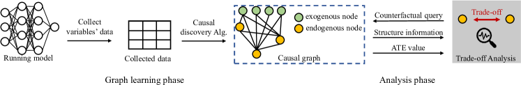
Figure 1: Study overview.

II-A Fairness-Improving Methods

A significant amount of research has been devoted to the investigation of fairness in ML [20, 21, 22, 23, 24, 3, 5, 6, 7, 25, 8, 4, 9, 26, 27, 28, 29, 30]. In general, most fairness-improving methods can be classified according to the ML stages when they are involved and the fairness objectives they aim to achieve [12, 31].

Methods by Different Stages. Fairness-improving methods can be categorized based on the stage of the machine learning pipeline they are involved in. These stages can be classified as pre-processing, in-processing, or post-processing methods. Pre-processing methods manipulate the training data, while in-processing methods modify the model during training. Post-processing methods, on the other hand, adjust the predictions made by the trained model. Representative methods for each type of fairness-improving method have been selected and analyzed in our study (see Table II for more information).

Methods by Different Objectives. Fairness-improving methods can also be categorized based on the fairness objectives they aim to achieve. Generally, there are two primary types of fairness objectives: individual fairness and group fairness. Individual fairness refers to treating all individuals equally. Zhang et al. [31] introduced the Causal Discrimination Score (CDS) to quantify the individual fairness of a model. On the other hand, group fairness focuses on the fairness of a model’s predictions for different groups defined by one or more sensitive attributes. A model is considered fair if it treats all subpopulations equally. Common group fairness metrics include Disparate Impact (DI) [23] and Statistical Parity Difference (SPD) [32], as presented in Table III.

Motivation. The different types of fairness-improving methods, along with their varied objectives, can introduce complexity and challenges in achieving a balanced solution. For instance, two well-known fairness objectives, group fairness and individual fairness, are often mutually incompatible, leading to an inevitable trade-off between them [13, 14]. A similar phenomenon is also observed in other objectives such as robustness versus accuracy [33]. These complex relationships behind potentially conflicting objectives render achieving a good trade-off among multiple metrics (fairness, accuracy, robustness) challenging. Overall, this research advocates the usage of causality analysis, a well-established and systematic approach, for understanding the complex relationships between variables presented in this fairness-improving context over ML pipeline. We envision that, by employing causality analysis, we can make the process of improving fairness notably more transparent and manageable. We present the preliminary knowledge of causality analysis in the following subsection.

II-B Causality Analysis

Causality analysis effectively provides a systematic and comprehensive understanding of the complex causal relationships between variables [34, 35, 36, 37]. This desirable feature is attained through two fundamental steps: causal discovery and causal inference.

According to Judea Pearl [15], causation (or causal relation) refers to the relationship between two variables, wherein changes in one variable cause changes in the other. This concept differs from correlation, which merely indicates the statistical dependence between two variables. Considering a simple example, $X\leftarrow Z\rightarrow Y$, where $X$ and $Y$ are correlated, but $X$ does not cause $Y$ (and vice versa). Here, $Z$ is a confounder because it simultaneously causes $X$ and $Y$. Indeed, the correlation between $X$ and $Y$ is induced by $Z$. This example highlights why correlation alone cannot imply causation. To address more complex cases, we introduce the definition of causal graph as follows:

Definition 1 (Causal Graph).

A causal graph (a.k.a., Bayesian network) is a directed acyclic graph (DAG) consisting of nodes $V$ and edges $E$, i.e., $G=(V,E)$, where each node $X$ ($X\in V$) represents a random variable and each edge $X\rightarrow Y$ ($X,Y\in V$) represents a directed causal relation from $X$ to $Y$. The nodes in the graph can be categorized into two groups: endogenous nodes, which are determined by the values of other nodes in the graph, and exogenous nodes, which are determined by external factors.

Causal graphs facilitate reasoning both qualitative and quantitative causal relations between variables. In practice, however, the causal graph is commonly unknown. For another, although causal relationships can be inferred if interventions are properly applied, the majority of real-world variables cannot be simply intervened [38]. This obstacle necessitates causal discovery, which aims to reconstruct the causal graph from observational data.

Causal Discovery. Causal discovery is the process of inferring a directed acyclic graph (DAG), where each node represents a variable and each edge represents a causal relation. Holistically, mainstream causal discovery methods can be categorized into three groups: constraint-based, score-based, and model-based methods [38]. Constraint-based methods use the conditional independence test to determine the edges and properties of special relationships (such as confounder) to infer the direction of causal relations [39, 40, 41, 42, 43, 44]. Score-based methods formulate causal discovery as a search problem and evaluate the quality of the causal graph using a score function [45, 46, 47, 48]. For model-based methods, asymmetry is exploited to identify causal relations [49, 50, 51].

Causal Inference. Causal inference quantitatively estimates the causal effect of one variable on another variable based on a causal graph. Although the causal graph is generally interpretable, estimating the causal effect can be challenging. Suppose, for instance, there are three variables $X$, $Y$, and $Z$, where $Z\rightarrow X\rightarrow Y$ and meanwhile $Z\rightarrow Y$. Here, it is challenging to accurately determine the true causal effect of $X$ on $Y$ while minimizing the impact of $Z$. In causality analysis, Average Treatment Effect (ATE) is commonly utilized to address this issue [15]. Below is the definition of ATE:

Definition 2 (ATE).

In causal graph $G$, ATE of $X$ on $Y$ can be computed as:

$$\textnormal{ATE}=\mathbb{E}[Y\mid do(X=\bm{x}_{1})]-\mathbb{E}[Y\mid do(X=\bm{x}_{2})]$$ (1)

where the $do(\cdot)$ operator denotes a counterfactual query, which represents a hypothetical intervention over the value of a variable $X$ (i.e., $X$ is set to a constant value $\bm{x}$, which may not be observed in the data). $\bm{x}_{1}$ and $\bm{x}_{2}$ are two arbitrary values of $X$ that are determined by the user.

Since ATE employs counterfactual queries, it cannot be explicitly estimated from observational data as it is a causal estimand. The process of making an incomputable causal estimand computable is known as causal inference [52]. This paper uses a popular causal estimation method, double machine learning (DML) [53]. Continuing with the preceding example, where $Z\rightarrow X\rightarrow Y$ and meanwhile $Z\rightarrow Y$. $X$ denotes the treatment variable, $Y$ denotes the outcome variable, and $Z$ denotes the confounder. DML uses two arbitrary machine learning models to estimate $X$ and $Y$ from $Z$, respectively. The effect of the confounder $Z$ can then be “removed” by estimating the difference between the predicted and observed values of $X$ and $Y$ (i.e., the residuals). DML makes no assumptions about the form of the confounder $Z$’s effect [54], making it applicable to a wide range of causal relations.

III Study Pipeline

Fig. 1 depicts our study workflow, which consists of two main phases: (1) graph model construction and (2) trade-off analysis. In the first phase, we collect a substantial quantity of data, which includes un-interventional observed metrics such as test accuracies and SPD scores, and interventional metrics like the fairness-improving methods’ parameters. Certain variables are referred to as “un-interventional” because their values cannot be directly changed by the user (e.g., the model test accuracy). We then use a causal discovery algorithm to learn a causal graph, where nodes represent variables (metrics and parameters), and directed edges represent causal relations between them.

In the second phase, we propose counterfactual queries according to the identified trade-off between two un-interventional nodes on the causal graph; these nodes typically include the metrics of model accuracy, fairness, and robustness. Our aim is to explain the underlying cause for the trade-off among these important metrics, thus providing insights into the influence of the ML fairness-improving methods over other important factors on the ML pipeline.

III-A Graph Model Construction

This study seeks to reveal the intricate relationships among diverse kinds of metrics. However, the sheer number of metrics and the complexity of the relationships between them pose considerable obstacles in learning a sufficiently precise causal graph. ➊ and ➋ illustrate how we address this challenge from the perspectives of data collection and graph learning.

➊ Collecting Training Data. Due to the limited number of variables (e.g., only 14 nodes are involved in Baluta et al.’s work [35]), prior works tend to focus on un-interventional variables. In contrast, because of the large number of variables involved in this problem, [35]’s practice fails to guarantee that the entire value range of each variable is exhaustively covered. Therefore, we introduce fairness-improving methods as interventional nodes in the causal graph. For parameter-tunable methods, we convert and normalize their parameters into a ratio, which ranges from 0 to 1. For non-parameter-tunable methods, we use probabilistic sampling, also converting them into ratios as the following equation shows.

$$D^{\prime}=T_{fair}(\alpha D)\cup(D-\alpha D)$$ (2)

where $D$ is the original dataset, $T_{fair}$ is the fairness-improving method, $\alpha$ denotes the ratio, $\alpha D$ presents the selected $\alpha$ part of the original dataset, $(D-\alpha D)$ denotes the remaining part, and $D^{\prime}$ is the resulting dataset by applying $T_{fair}$ on the $\alpha$ part. Accordingly, all fairness-improving methods can be represented as a ratio and can be treated as nodes in the causal graph. By intervening these nodes, we can collect sufficient, high-quality training data for causal discovery, with all possible value ranges of un-interventional variables covered.

➋ Learning Causal Graph. We employ DiBS [47], a state-of-the-art score-based method, to learn causal graph with variational inference and is more efficient than other methods that rely on Markov chain Monte Carlo (MCMC) sampling. As will be shown in Sec. V, DiBS is able to accurately learn causal graphs and aligns well with expert knowledge.

III-B Trade-off Analysis

From a holistic perspective, the influence of a specific fairness-improving method can be considered as a change propagation throughout the causal graph. Initially, the parameters of fairness-improving methods, denoted as a node on the causal graph, directly affect their children nodes, which subsequently leads to indirect impacts on their descendants. As a consequence of this influence propagation, various descendants might experience either improvements or downgrades.

When examining a pair of metrics ($X$ and $Y$) that are affected distinctively by the fairness-improving method, it becomes essential to comprehend the trade-off between $X$ and $Y$. Although the causal graph has offered a qualitative view of the relationships between metrics and fairness-improving methods (e.g., one method affects a metric), it is not sufficient to accurately quantify the trade-off involving two specific metrics. For instance, we may first observe “Test Accuracy” decreases while “Test SPD” (Statistical Parity Difference) increases after applying, Reweighing [20], a fairness-improving method (see details in Table II). Then, on the causal graph, we observe that “Test Accuracy” and “Test SPD” has a common ancestor “Dataset SPD” (SPD of the dataset). However, without further analysis, we are unable to conclude if the trade-off is caused by “Dataset SPD” or by other factors (e.g., other common ancestors). In the following section, we will first provide a formal definition of the trade-off that occurs between two metrics. Then, we will show how a trade-off can be explained by the combination of causal graphs and ATE analysis.

Trade-off Definition. In line with prior works [55, 56, 31], we define the concept of trade-off: a situation where an effort to enhance one aspect of a system (i.e., an endogenous node in our research context) results in a downgrade in another aspect. The quantifiable effect of one metric on another can be precisely measured using average treatment effect (ATE), enabling the identification of potential causes for the trade-off.

To adequately define whether a change in one metric is an enhancement or downgrade, we introduce a user-defined function ${\color[rgb]{0,0,1}\textit{{sign}}}:\mathbb{R}\times\mathbb{R}\to\{+,-\}$. This function takes the current value and the change of a metric as input, and outputs the corresponding sign of the change (“$+$” indicating an improvement and “$-$” indicating a downgrade). It is worth noting that the definition of ${\color[rgb]{0,0,1}\textit{{sign}}}(\cdot,\cdot)$ is specific to each metric. For instance, in the case of accuracy, ${\color[rgb]{0,0,1}\textit{{sign}}}_{\text{Acc}}(0.6,0.1)$ yields “$+$” to demonstrate that the accuracy has improved due to the change. Conversely, for the SPD score, ${\color[rgb]{0,0,1}\textit{{sign}}}_{\text{SPD}}(0.6,0.1)$ yields “$-$” to illustrate that the statistical parity difference has been downgraded as a result of the change. Then, given two metrics $X$ and $Y$ and a fairness-improving method $T$, there is a trade-off between $X$ and $Y$ if and only if ${\color[rgb]{0,0,1}\textit{{sign}}}_{X}(x_{T=0},\text{ATE}^{x}_{t})\neq{\color[rgb]{0,0,1}\textit{{sign}}}_{Y}(y_{T=0},\text{ATE}^{y}_{t})$, where $x_{T=0}$ and $y_{T=0}$ are the values of $X$ and $Y$ before applying $T$, respectively, and $\text{ATE}^{x}_{t}$ and $\text{ATE}^{y}_{t}$ are the ATEs of $T$ on $X$ and $Y$, respectively. This condition indicates that the fairness-improving method $T$ has distinct effects on $X$ and $Y$.

Input: Causal Graph $G$, Fairness Improving Method $T$, two Metrics $X$ and $Y$.

Output: Trade-off causes list $C$

1 $C\leftarrow\emptyset$;

2 $\text{ATE}^{x}_{t}\leftarrow\mathbb{E}[X\mid do(T=1)]-\mathbb{E}[X\mid do(T=0)]$;

3 $\text{ATE}^{y}_{t}\leftarrow\mathbb{E}[Y\mid do(T=1)]-\mathbb{E}[Y\mid do(T=0)]$;

4 $x_{T=0}\leftarrow\mathbb{E}[X|T=0]$; $y_{T=0}\leftarrow\mathbb{E}[Y|T=0]$;

5 if ${\color[rgb]{0,0,1}\textit{{sign}}}_{X}(x_{T=0},\text{ATE}^{x}_{t})={\color[rgb]{0,0,1}\textit{{sign}}}_{Y}(y_{T=0},\text{ATE}^{y}_{x}$) then

6       return $\bot$; // Terminate the algorithm in the absence of trade-offs.

7      

8 end if

9if $X$ causes $Y$ on $G$ then

10       $x_{T=1}\leftarrow\mathbb{E}[X|T=1]$;

11       $\text{ATE}^{y}_{x}\leftarrow\mathbb{E}[Y\mid do(X={x_{T=1}})]-\mathbb{E}[Y\mid do(X=x_{T=0})]$;

12       if ${\color[rgb]{0,0,1}\textit{{sign}}}_{X}(x_{T=0},\text{ATE}^{x}_{t})\neq{\color[rgb]{0,0,1}\textit{{sign}}}_{Y}(y_{T=0},\text{ATE}^{y}_{x})$ then  $C\leftarrow C\cup\{X\}$ ;

13      

14 end if

15else if $Y$ causes $X$ on $G$ then

16       $y_{T=1}\leftarrow\mathbb{E}[Y|T=1]$;

17       $\text{ATE}^{x}_{y}\leftarrow\mathbb{E}[X\mid do(Y=y_{T=1})]-\mathbb{E}[X\mid do(Y=y_{T=0})]$;

18       if ${\color[rgb]{0,0,1}\textit{{sign}}}_{Y}(y_{T=0},\text{ATE}^{y}_{t})\neq{\color[rgb]{0,0,1}\textit{{sign}}}_{X}(x_{T=0},\text{ATE}^{x}_{y})$ then  $C\leftarrow C\cup\{Y\}$ ;

19      

20 end if

21$P_{C}\leftarrow\text{FindPotentialCause}(G,X,Y)$;

22 foreach $P\in P_{C}$ do

23       $p_{T=1}\leftarrow\mathbb{E}[P|T=1]$; $p_{T=0}\leftarrow\mathbb{E}[P|T=0]$;

24       $\text{ATE}^{x}_{p}\leftarrow\mathbb{E}[X\mid do(P=p_{T=1})]-\mathbb{E}[X\mid do(P=p_{T=0})]$;

25       $\text{ATE}^{y}_{p}\leftarrow\mathbb{E}[Y\mid do(P=p_{T=1})]-\mathbb{E}[Y\mid do(P=p_{T=0})]$;

26       if ${\color[rgb]{0,0,1}\textit{{sign}}}_{X}(x_{T=0},\text{ATE}^{x}_{p})\neq{\color[rgb]{0,0,1}\textit{{sign}}}_{Y}(y_{T=0},\text{ATE}^{y}_{p})$ then  $C\leftarrow C\cup\{P\}$ ;

27      

28 end foreach

return $C$

Algorithm 1 Analysis

Trade-off Analysis. The process of performing trade-off analysis is described in Alg. 1. Overall, Alg. 1 accepts a causal graph $G$ (generated in ➋ of Sec. III-A), a fairness-improving method $T$, and two metrics $X$ and $Y$ (lines 1–2). It returns a list of identified causes for the trade-off between $X$ and $Y$ (line 25), where each cause (can be $X$ or $Y$ itself) represents one node on the causal graph. Following the above trade-off definition and the usage of $T=0$, we note that $T=1$ in Alg. 1 indicates that the fairness-improving method $T$ is applied.

When provided with two metrics $X$ and $Y$, Alg. 1 initially checks for the existence of a trade-off between them, based on the trade-off definition we just present (lines 2–7). And if a trade-off is present, the algorithm proceeds. Subsequently, if $X$ is a cause of $Y$ (i.e., there exists a path from $X$ to $Y$ in the causal graph $G$), Alg. 1 computes the ATE of $X$ on $Y$ (lines 9–10) and verifies whether the trade-off is caused by $X$ (lines 11–12). Likewise, if $Y$ is a cause of $X$, Alg. 1 repeats the process with reversed roles (lines 13–17). Finally, Alg. 1 queries the causal graph to identify the potential causes of the trade-off, which are the common ancestors of $X$ and $Y$ (line 18). For each potential cause (line 19), Alg. 1 calculates its ATE on both $X$ and $Y$ (lines 21–22). If the ATEs implies a trade-off, the potential cause is designated as a cause (line 23).

IV Experiment Setup

Our study is implemented in Python with roughly 2.8K lines of code. All experiments are launched on one AMD CPU Ryzen Threadripper 3970X and one NVIDIA GPU GeForce RTX 3090.

TABLE I: Dataset information.

Dataset	Size	Favorable	Sensitive	Privileged
		Class	Attribute	Group
Adult [16]	48,842$\times$12	income$>$50K	sex	sex=Male
			race	race=White
COMPAS [17]	7,214$\times$11	no recidivism	sex	sex=Female
			race	race=Caucasian
German [18]	1,000$\times$21	good credit	sex	sex=male
			age	age$>$30

IV-A Datasets & Model

Dataset. Our experiments are conducted on three real-world datasets: Adult [16], COMPAS [17], and German [18]. These datasets are widely used for fairness research [31, 57, 7, 8, 9]. Table I shows the information of these datasets. Each of them has two sensitive attributes, which smoothly enables analyzing the trade-off between multiple sensitive attributes’ fairness.

Model Training. Following Zhang et al. [31], we use a feed-forward neural network (FFNN) with five hidden layers. To adjust the model’s learning capacity, we control its size with a variable, model width. The default value of this variable is $4$, so layers of the model contain $4\times 16=64$, $4\times 8=32$, $4\times 4=16$, $4\times 2=8$, and $4\times 1=4$ neurons, respectively. For each dataset presented in Table I, we split the data into training and test sets with a ratio of 7:3. All trained models possess comparable performance [31, 8, 4, 9]. In particular, we achieve 84.7% accuracy on the Adult Income dataset, 67.4% accuracy on the COMPAS dataset, and 72.1% accuracy on the German Credit dataset. We also clarify that this model architecture is sufficient for our experiments, as all three datasets contain a relatively small number of features (see Table I).

TABLE II: Fairness improving methods.

Category	Name
Pre-processing (6)	Reweighing [20]
	Disparate Impact Remover (DIR) [23]
	FairWay [7]
	FairSmote [8]
	FairMask [4]
	LTDD [9]
In-processing (3)	Adversarial Debiasing (AD) [5]
	Prejudice Remover (PR) [21]
	Exponentiated Gradient Reduction (EGR) [6]
Post-processing (3)	Reject Option Classification (ROC) [22]
	Equalized Odds (EO) [58]
	Calibrated Equalized Odds (CEO) [3]

IV-B Fairness Improving Methods

Table II presents the fairness-improving methods used in our experiments. It is notable that we have opted for significantly more pre-processing methods than the other categories. This decision is influenced by the trend in the software engineering community and the greater compatibility offered by pre-processing methods. In particular, we surveyed top-tier conferences/journals in the software engineering community and found that pre-processing methods are generally dominant this line of research. Moreover, these methods impose no constraints on the model and have no impact on its output.

Conversely, some in-processing methods are designed for specific models, such as FairNeuron [10] that only works on particular DNNs provided by the authors. This makes in-processing less compatible and impedes a fair comparison with other methods. Post-processing methods usually alter the model’s output, nullifying prediction probability and prohibiting robustness-related analysis, such as adversary attacks. Given that said, as a comprehensive study, we still select three representative methods from both in-processing and post-processing methods.

IV-C Metrics

This paper employs a wide range of metrics to evaluate model performance, fairness (both individual and group), and robustness. We present the metrics used in our experiments in Table III to ensure clarity. For detailed definitions of each metric, interested readers may refer to the cited references.

TABLE III: Metrics information.

Category	Name
Performance (2)	Accuracy (Acc) [59]
	F1 score (F1) [59]
Group Fairness (3)	Disparate Impact (DI) [59]
	Statistical Parity Difference (SPD) [59]
	Average Odds Difference (AOD) [59]
Individual Fairness (3)	Consistency (Cons) [60]
	Theil Index (TI) [60]
	Causal Discrimination Score (CDS) [31]
Robustness (4)	FGSM’s Success Rate (FGSM) [61]
	PGD’s Success Rate (PGD) [62]
	Rule-Based MI’s Accuracy (Rule) [63]
	Black-Box MI’s Accuracy (Bbox) [63]

Except for the Causal Discrimination Score (CDS), all fairness metrics are computed by the widely-used AIF360 [64]. We implement the CDS metric by us. For robustness, we evaluate the model from two perspectives: adversarial attack [61, 62] and membership inference (MI) attack [63]. For the adversarial attack, we use two standard approaches, the Fast Gradient Sign Method (FGSM) [61] and the Projected Gradient (PGD) [62]. Here, the success rate is defined as the ratio of the number of adversarial examples that successfully fool the model to the total number of adversarial examples. In our experiments, the FGSM/PGD implementation provided in Torchattacks [65] is used. For the membership inference attack, we use two popular methods: the rule-based and black-box methods. The rule-based method assumes that a sample is a member if the model correctly predicts its label; otherwise, the sample is a non-member. The black-box method trains a model to predict whether a sample is a member or not. Both methods are implemented by ART [66].

Although users are typically only interested in metrics measured on the test set, we also measure dataset properties (e.g., DI of the dataset) and metrics on the training set (e.g., SPD model’s prediction on the training set). We regard these metrics as intermediate nodes, such as when pre-processing methods alter the dataset’s properties, causing a change in the model’s prediction on the training set, which in turn causes a change in the model’s prediction on the test set. Therefore, these mediators contribute to causal graph learning. In addition, we measure fairness metrics for two sensitive attributes, respectively, to analyze the trade-off between multiple sensitive attributes. Overall, the causal graph contains 46 nodes.

V Pilot Study on Causal Graph Quality

Before using the learned causal graph to answer RQs (Sec. VI), we study their accuracy through a pilot study. This section consists of two pilot tasks: graph comparison and accuracy verification. In the first task, we compare the six learned causal graphs (three datasets $\times$ two sensitive attributes in each dataset) to find their similarities and differences. In the second task, we conduct a human evaluation and a quantitative analysis to verify the accuracy of the learned causal graphs.

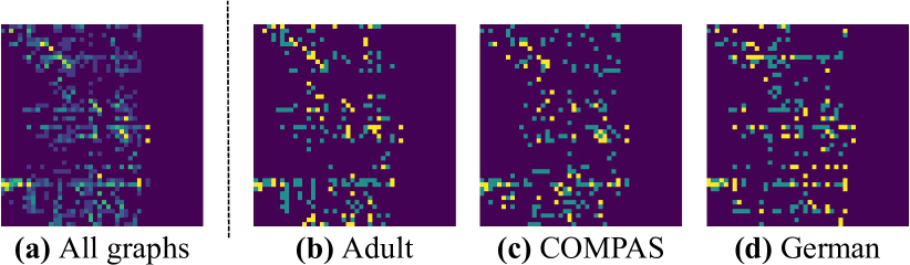
Figure 2: Overlap between the learned causal graph. The brighter the color, the higher the overlap.

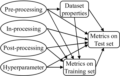
Figure 3: High-level common patterns across all graphs.

V-A Graph Comparison

From Fig. 2(a), we can see that the overlap across all graphs is small. These six graphs reach consensus on only 14 edges, while the average number of edges per graph is 138. According to previous research [35], this enormous distinction is a common phenomenon in causal discovery, compelling us to learn six graphs instead of one in this study. We clarify that the relationships among variables are typically more complex than we believe, as there is no simple equation to characterize them (e.g., the relationship between model loss and SPD score). Therefore, the causal graph may change considerably if the dataset, model architecture, or even the sensitive attribute addressed in this study is altered. In fact, as expected, when we retain the same dataset and model architecture, we can observe that the overlap increases. In Fig. 2(b), (c), and (d), the overlaps between two graphs range from 30% to 50%.

Despite the intuitive observation, we clarify that the small overlaps between the learned causal graphs, as reflected in Fig. 2, does not imply that there is no common pattern across those graphs. For instance, we can observe that the right parts of all graphs are “empty” (colored in dark purple), signifying that nodes corresponding to those right parts lack parents. This is because those nodes represent the fairness-improving methods. As interventional variables, they are exogenous nodes in the graph. Based on this kind of observation, we conclude a high-level common pattern across all graphs, as shown in Fig. 3. This pattern is consistent with our expectations, such that the pre-processing methods cause the change in the data, which subsequently affect the model performance. Overall, we view that the pilot study at this step demonstrates the high accuracy of the learned causal graphs.

V-B Accuracy Verification

As the study basis, the accuracy of the learned causal graphs is essential to the effectiveness of the entire pipeline. Because of the absence of ground truth, we propose a human evaluation to assess the quality and accuracy of learned causal graphs. In particular, we invite six experts in the field of software engineering (all of whom are Ph.D. students with extensive experience in fairness or ML) to evaluate the causal graphs.

Since there are 46 nodes in each graph, indicating high complexity and a large number of edges, we presume that it is impractical to request that experts construct causal graphs from scratch. Instead, the knowledge and experience of experts are more suitable for validating the causal graphs learned by the causal discovery algorithm. Specifically, for each learned causal graph, we randomly sample three subgraphs (each containing 15 nodes out of 46 nodes in total) and present them to the experts for evaluation. Experts are requested to mark any edges on the subgraph they disagree with and to note any edges not present in the subgraph that should be included. Then, we gather this feedback and compute an error rate (i.e., the rate of incorrectly discovered edges by DiBS) and a negative predictive value (NPV; denoting the proportion of absent edges in the learned graph).

TABLE IV: Human evaluation.

		nodes	edges	error rate	NPV
Adult	sex	46	141	1.78%	6.84%
	race	46	136	4.77%	4.15%
COMPAS	sex	46	130	10.19%	2.30%
	race	46	133	7.90%	3.39%
German	sex	46	141	6.71%	3.69%
	age	46	146	5.73%	2.58%

The results are shown in Table IV. We can see that the error rate is less than 10% in the vast majority of instances (with only one exception that trivially exceeds 10% by 0.19%), where the lowest value is only 1.78%. The results for NPV are even more impressive. In all cases, the NPV is less than 7%, with a minimum value of 2.30%. This result indicates that the learned causal graphs are highly accurate and can serve as the foundation for further analysis.

TABLE V: Ablation study results.

		Full ver.	w/o pre	w/o in	w/o post	w/o all
Adult	sex	1.00	0.56	0.64	0.77	0.00
	race	1.00	0.43	0.81	0.82	0.00
COMPAS	sex	1.00	0.55	0.90	0.89	0.00
	race	1.00	0.48	0.89	0.88	0.00
German	sex	1.00	0.65	0.54	0.76	0.00
	age	1.00	0.60	0.67	0.81	0.00

In addition to the human evaluation, we also report the statistics of the learned causal graphs and their ablated versions in Table V, where “Full ver.” represents that all fairness-improving methods are included, and “w/o XX” indicates that some of the fairness-improving methods are excluded (e.g., “w/o pre” means pre-processing methods are excluded). We use normalized Bayesian Gaussian equivalent (BGe) score [67, 68], whose implementation is provided by DiBS [47], to measure the quality of the learned causal graph. As a standard metric in causal discovery, BGe scores reflect the data-fitness of the graph. The higher the BGe score, the better the learned graph. Note that BGe scores are data-specific, i.e., they cannot be compared across different scenarios, so we only compare the BGe scores on the same row in Table V.

The results indicate that the application of fairness-improving techniques has a substantial impact on the quality of the learned causal graphs. Furthermore, each category of fairness-improving methods is essential to the quality of the learned causal graph, as removing any category of fairness-improving methods will result in a significant drop in the BGe scores.

VI Evaluation

We now investigate the mechanisms underlying various trade-off phenomena related to fairness, including the trade-off between fairness and model performance (RQ1), the trade-off between multiple sensitive attributes (RQ2), and the trade-off between fairness and model robustness (RQ3). In each RQ, we first present the discovered trade-off (with counts of occurrences) and corresponding causes that are revealed by Alg. 1 using the learned graphs. Then, we analyze the causes and discuss the implications of the trade-off and their causes.

For the sake of space, metric names are abbreviated as follows: prefix-metric, where prefix is either Tr (measured on training data), Te (measured on testing data), or D (datasets’ properties), and metric follows the same naming convention as in Table III. Additionally, Width denotes the width of the neural network, which is the hyperparameter that controls the number of neurons in each layer. Using Tr-SPD as an illustration, it represents “SPD” (Statistical Parity Difference; see Table III) measured on the training set. Note that the term “causes” refers exclusively to the metrics mentioned in Sec. IV-C. All fairness-improving methods are excluded from “causes”, as they are undoubtedly viewed as the causes of the trade-offs triggered by themselves. We clarify that the purpose of this study is to analyze the mechanisms underlying the trade-offs, so we concentrate on the intricate relationships among metrics.

Processing Time. Building each causal graph requires approximately 30 minutes to learn from the data. As for the trade-off analyses (depicted in Alg. 1), we report that the average processing time for analyzing each trade-off is less than 1 minute, the majority of which is spent on computing the ATEs. In studying the following RQs, the processing time of computing ATEs is negligible, typically less than 20 seconds.

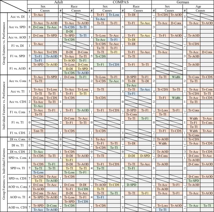
Figure 4: Trade-offs between fairness and model performance. The color of each cell indicates the confidence of revealed causes. In particular, red indicates a full confidence (100%), yellow indicates a high confidence (70%–99%), green indicates a medium confidence (30%–69%), and blue indicates a low confidence (1%–29%).

VI-A RQ1: Fairness vs. Model Performance

As mentioned in Sec. II, there are two types of fairness: group fairness and individual fairness. This section explores the trade-offs between both types of fairness and model performance, i.e., group fairness vs. model performance and individual fairness vs. model performance. Additionally, we also investigate the trade-offs between group fairness and individual fairness, as this is a topic that has been primarily focused in the fairness literature [55, 56, 31].

Fig. 4 reports the observed trade-offs for each scenario in the form of “counts (#)” and “causes”. The “counts” column shows the trigger time of trade-offs w.r.t. fairness-improving methods in Table II. For instance, the “counts” of “Acc vs. DI” is $1$, when “sex” is the addressed sensitive attribute on the “Adult” dataset. This means that there is only one fairness-improving method that triggers the trade-off between Accuracy and DI on Adult. The “causes” column shows the causes of the trade-offs, which are revealed by Alg. 1. For each cause, we also report the “confidence” (i.e., the percentage of the trade-off caused by the metric) in four colors. Additionally, we use a diagonal line when no causes are found.

Fig. 4 provides a comprehensive view of the trade-offs between fairness and model performance by listing all observed trade-offs. As the count of the majority of trade-offs is not zero, this table demonstrates that “trade-off” is a common phenomenon in fairness-improving methods. Moreover, the kinds of trade-offs vary considerably across different scenarios. For example, in the case of group fairness vs. performance, we observe that the trade-offs observed on Adult are mainly between SPD and performance metrics (the trade-off between Accuracy and SPD is observed eight times, and the trade-off between F1 and SPD is observed seven times when sex is the addressed sensitive attribute). In contrast, on COMPAS, most trade-offs are observed between AOD and performance metrics. This result suggests that the selection of fairness metrics may have a substantial impact on the number and type of trade-offs that can be observed.

We presume that the more frequently a metric is observed as a cause, the more important the metric is, as it is more likely to reveal how well the fairness-improving method works with regard to the trade-off, i.e., whether this method achieves a win-win situation. Based on this presumption, we expect to identify the most informative and beneficial metric for the development of fair ML based on the results of our experiments. From Fig. 4, we observe that there is no unified cause for all trade-offs. Instead, the causes of trade-offs vary considerably across different scenarios. Furthermore, the distribution of causes is not uniform. In Fig. 4, the most prevalent causes of trade-offs are metrics measured on the training set (e.g., Tr-TI). This type of metric functions as a cause for trade-offs 190 times, which is far more than other types of causes. In comparison, metrics measured on the test set (e.g., Te-TI) are only 38 times the cause of trade-offs, and for metrics of datasets’ properties, the number is 29. This significant difference motivates us to investigate the distribution of causes further.

TABLE VI: Distribution of causes in RQ1.

		Data	Train	Test	Total
Group	DI	8	6	0	14
	SPD	4	8	1	13
	AOD	N/A	30	0	30
Individual	Cons	17	6	0	23
	TI	N/A	21	21	42
	CDS	N/A	36	0	36
Total		29	107	22	158

Table VI presents the distribution of causes. In this table, we report the frequency of each fairness metric being the causes of trade-offs listed on Fig. 4. The column indicates the phase in which the metric is measured, i.e., “Data” for the dataset’s properties, “Train” for the training set, and “Test” for the test set. Note that AOD, TI, and CDS depend on the model’s prediction, so they are N/A for the “Data” column. This table reveals that AOD is the most common cause of trade-offs among all group fairness metrics, occurring 30 times. For individual fairness, TI is the most common cause of trade-offs, observed 42 times. Also, individual fairness metrics generally cause trade-offs more frequently than group fairness metrics.

RQ1 Findings: In this RQ, we have the following two suggestions for users and developers of fair ML.

1. For the users, they should be aware that the results of experiments for fairness-improving methods may be biased by the selection of metrics. Moreover, the metrics that work well in one scenario to discover the trade-offs may not work well in other scenarios. To obtain a more comprehensive and faithful understanding of the fairness-improving method, we recommend that users use sufficient metrics or our causality analysis-based method, to explore the presumably optimal choice of metrics for their scenarios.

2. For the developers, we suggest that they pay closer attention to the metrics measured on the training set, as they are the most common causes of trade-offs according to our study. Additionally, we recommend AOD among all group fairness metrics and TI among all individual fairness metrics.

VI-B RQ2: Multiple Sensitive Attributes

In this RQ, we investigate the trade-offs between multiple sensitive attributes. For the sake of space, we only report the results of experiments on COMPAS, and present other results on the website [69]. To distinguish metrics measured on different sensitive attributes, we change the abbreviation of metrics to “prefix-sensitive attribute-metric”. For example, “Tr-Sex-SPD” represents “SPD” measured on the training set with “Sex” as the sensitive attribute. In this RQ, only the trade-offs between group fairness for different sensitive attributes are considered, as individual fairness metrics are not related to the sensitive attribute.

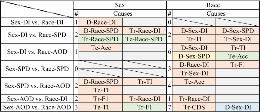
Figure 5: Trade-offs between multiple sensitive attributes.

Fig. 5 presents the results of experiments on COMPAS. The left part of this table shows the results when the addressed sensitive attribute of the fairness-improving method is set to “Sex”, and the right part shows the results when the sensitive attribute is set to “Race”. Although these two parts attain consensus in some cases (e.g., they both agree that the trade-off between “Sex-DI” and “Race-DI” is rare), they have several substantial differences. For example, the left part reveals that the trade-off is rare between “Sex-DI” and “Race-AOD” (the “counts” is only one), whereas the right part shows that the trade-off is frequent between these two metrics (six counts). To explain this difference, we present the causal graphs of these two metrics in Fig. 6.

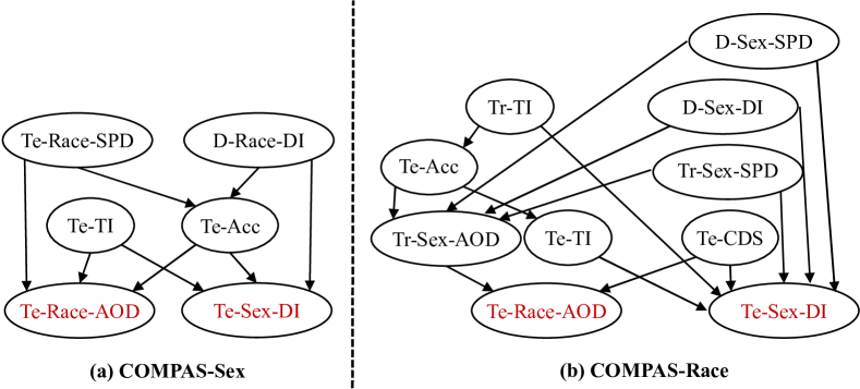
Figure 6: A comparison between trade-offs in different scenarios.

This figure provides an intuitive explanation for the aforementioned distinction. Clearly, the causal graph of the scenario “COMPAS-Race” is more intricate than that for “COMPAS-Sex”. With more common ancestors in the graph, it is more likely that more causes leading to trade-offs will be identified. In addition, Fig. 6 also explain the difference in found causes between “COMPAS-Sex” and “COMPAS-Race”. In Fig. 6(a), the metric “Te-Acc” not only has direct causal relations with “Sex-DI” and “Race-AOD”, but also mediates the effect from “Te-Race-SPD” and “D-Race-DI” to “Sex-DI” and “Race-AOD”. Therefore, “Te-Acc” is the cause with full confidence here. In contrast, “Te-Acc” no longer has direct causal relation with either “Sex-DI” or “Race-AOD” in Fig. 6(b). This explains why its confidence decreases drastically in scenario “Compas-Race”.

RQ2 Findings: We observe the substantial variation in patterns of trade-offs between different sensitive attributes even on the same dataset. Furthermore, we take a pair of causal graphs as an example to explain the difference in detail.

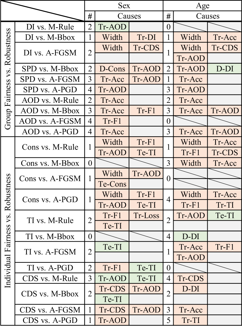
Figure 7: Trade-offs between fairness and model robustness.

VI-C RQ3: Fairness vs. Model Robustness

As essential properties of ML models, both fairness and robustness receive considerable attention in the research community. Although some works [70, 71, 72] examine them simultaneously, no one has systematically studied the trade-offs between them. This RQ investigates the trade-offs between fairness and model robustness. Similar to RQ2, we only report the results of experiments conducted on German in Fig. 7 and present the remaining results on the website [69]. For the abbreviation of robustness metrics, we use “prefix-robustness metric” to represent them, where prefix is either “A” (adversarial attack) or “M” (membership inference).

Comparing patterns of trade-offs in Fig. 7 with those in Fig. 4, an apparent distinction is that the hyperparameter “Width” causes much more trade-offs than it does in Fig. 4’s same scenario (“German-Sex” and “German-Age”). We interpret this difference as reasonable because the robustness metrics are more sensitive to the model’s learning ability and the degree of overfitting. Hence, it is not unexpected to see that performance metrics, including Accuracy and F1 score, also cause more trade-offs in Fig. 7. This result is consistent with research on membership inference [73, 74, 35].

It is evident to conclude that trade-offs between fairness and robustness are inevitable, given that fairness-improving techniques typically have a significant impact on the model’s performance. Moreover, the large number of observed trade-offs in Fig. 7 further suggests that the trade-offs between fairness and robustness should be taken seriously. Therefore, we suggest that future research on fairness-improving methods should consider this kind of trade-off, and faithfully disclose the results of potential robustness downgrades. We also clarify that the additional effort required to consider robustness will not be excessive, as Fig. 7 shows that the recommended metrics in RQ1 (AOD among group fairness metrics and TI among individual fairness) are still highly effective to inspect trade-offs between fairness and robustness.

RQ3 Findings: Fairness and robustness contain inevitable trade-offs. We advocate taking into account robustness metrics when designing fairness-improving methods, and we have illustrated that the extra cost is moderate.

VII Downstream Application

As detailed in Sec. VI, our method delivers a comprehensive and in-depth understanding of the trade-offs among multiple metrics. Naturally, the identified causal graph provides valuable insights into the selection of the optimal fairness-improving method for a given scenario. As a “by-product”, in this section, we present a case study that highlights the versatile application of our method in fairness-improving approach selection.

The case study is conducted on all datasets mentioned in Table I, specifically examining the interplay of accuracy, SPD, and consistency as key factors to consider in selecting a suitable fairness-improving method. Specifically, we first identify the causes of the trade-offs between the selected metrics. Then, we find the optimal value of each cause using ATE, which constitutes the optimal setting for fairness-improving methods. We compare our method against the Adaptive Fairness Improvement (AFI) [31], a state-of-the-art approach, which is tailored for this task and is not designed for trade-off analysis.

TABLE VII: Comparison of AFI vs. our method on fairness-improving method selection. Each cell of AFI and ours reports the difference compared to the default model (w/o FI). Green and brown indicate an improvement/downgrade, respectively.

		Adult		COMPAS		German
		Sex	Race	Sex	Race	Sex	Age
Acc	w/o FI	.8500	.8489	.6727	.6740	.7233	.7197
	AFI	-.0101	-.0167	-.0032	-.0050	-.0046	-.0050
	Ours	-.0138	-.0205	+.0098	+.0072	+.0100	+.0310
$|$SPD$|$	w/o FI	.1730	.0974	.1575	.1609	.0685	.0915
	AFI	-.0608	-.0299	-.1161	-.0926	-.0228	-.0321
	Ours	-.1718	-.0936	-.1488	-.1397	-.0658	-.0548
Cons	w/o FI	.9600	.9593	.9080	.9098	.7914	.8036
	AFI	-.0236	-.0101	-.0074	-.0061	-.0013	-.0100
	Ours	+.0179	+.0050	+.0081	+.0151	+.0215	+.0364

We report the evaluation results in Table VII. In particular, we find that our method surpasses AFI in almost all scenarios. This is reasonable: AFI can only select a single fairness-improving method, while our method can effectively combine multiple fairness-improving methods using the causal graph. For example, for the German-Age scenario, we found that the optimal combination of fairness-improving methods was to use both disparate impact remover (DIR) and predictive rate (PR), with their respective ratios set to 0.6 and 0.2. However, the limitation of AFI results in reduced effectiveness.

VIII Related Work

Trade-off Study in ML Fairness. Prior works have investigated the trade-offs associated with fairness. The analyzed trade-offs include fairness vs. accuracy [75, 55, 56, 76, 77, 78, 79], group fairness vs. individual fairness [13, 14], and fairness vs. robustness [70, 71, 72]. Typically, these studies have three primary goals: (1) establishing the theoretical existence of trade-offs, (2) designing methods to achieve optimal trade-offs, and (3) identifying the best trade-off through empirical comparisons. No one has, however, systematically analyzed the influence of fairness-improving methods over ML pipelines, as measured by the metrics in Sec. IV-C, to cast light on the causes of trade-offs.

Causality Analysis in SE. Recent years have witnessed a growing interest in applying causality analysis to SE. The high interpretability of causal graphs makes them appealing for a variety of SE problems, including software configuration [34], root cause analysis [80, 81, 82], and deep learning testing/repairing [83, 31, 84]. We have compared with AFI in Sec. VII to highlight the distinct focus and superior performance.

IX Threat to Validity

Internal Validity. The increase in the number of nodes in the causal graph may facilitate the discovery of causal relations, but it has a substantial impact on the computational cost. To balance the trade-off, we select 12 widely-used fairness-improving methods and 12 representative metrics. We presume that the number of nodes is sufficient to guarantee the accuracy of our analysis. Regarding users of the proposed analysis framework, they are encouraged to tailor the selection of nodes to their specific requirements. In terms of causal discovery, we employ DiBS, a state-of-the-art causal discovery algorithm, to infer causal graphs. Although DiBS outperforms other algorithms [47], it may not always identify the true causal graphs. To mitigate this threat, we use human evaluation in our pilot study for validating the derived causal graphs. In the future, we will attempt to combine graphs learned by one or multiple state-of-the-art algorithms to further improve the quality of causal graphs.

External Validity. Our study focuses on neural networks, possibly limiting generalizability to other ML models. However, given the popularity of neural networks and their strong compatibility with numerous fairness-improving methods, we argue that our results hold considerable value. To further alleviate this threat, we conduct experiments across various network architectures and datasets.

X Conclusion

This research analyzes the trade-offs among multiple factors in fair ML via causality analysis. We propose a set of design principles and optimizations to facilitate an effective usage of causality analysis in this field. With extensive empirical analysis, we establish a comprehensive understanding of the interactions among fairness, performance, and robustness.

References

- [1] T. Bono, K. Croxson, and A. Giles, “Algorithmic fairness in credit scoring,” Oxford Review of Economic Policy, vol. 37, no. 3, pp. 585–617, 2021.
- [2] R. Berk, H. Heidari, S. Jabbari, M. Kearns, and A. Roth, “Fairness in criminal justice risk assessments: The state of the art,” Sociological Methods & Research, vol. 50, no. 1, pp. 3–44, 2021.
- [3] G. Pleiss, M. Raghavan, F. Wu, J. Kleinberg, and K. Q. Weinberger, “On fairness and calibration,” Advances in neural information processing systems, vol. 30, 2017.
- [4] K. Peng, J. Chakraborty, and T. Menzies, “Fairmask: Better fairness via model-based rebalancing of protected attributes,” IEEE Transactions on Software Engineering, 2022.
- [5] B. H. Zhang, B. Lemoine, and M. Mitchell, “Mitigating unwanted biases with adversarial learning,” in Proceedings of the 2018 AAAI/ACM Conference on AI, Ethics, and Society, 2018, pp. 335–340.
- [6] A. Agarwal, A. Beygelzimer, M. Dudík, J. Langford, and H. Wallach, “A reductions approach to fair classification,” in International Conference on Machine Learning. PMLR, 2018, pp. 60–69.
- [7] J. Chakraborty, S. Majumder, Z. Yu, and T. Menzies, “Fairway: a way to build fair ml software,” in Proceedings of the 28th ACM Joint Meeting on European Software Engineering Conference and Symposium on the Foundations of Software Engineering, 2020, pp. 654–665.
- [8] J. Chakraborty, S. Majumder, and T. Menzies, “Bias in machine learning software: Why? how? what to do?” in Proceedings of the 29th ACM Joint Meeting on European Software Engineering Conference and Symposium on the Foundations of Software Engineering, 2021, pp. 429–440.
- [9] Y. Li, L. Meng, L. Chen, L. Yu, D. Wu, Y. Zhou, and B. Xu, “Training data debugging for the fairness of machine learning software,” in Proceedings of the 44th International Conference on Software Engineering, 2022, pp. 2215–2227.
- [10] X. Gao, J. Zhai, S. Ma, C. Shen, Y. Chen, and Q. Wang, “Fairneuron: improving deep neural network fairness with adversary games on selective neurons,” in Proceedings of the 44th International Conference on Software Engineering, 2022, pp. 921–933.
- [11] G. Tao, W. Sun, T. Han, C. Fang, and X. Zhang, “Ruler: discriminative and iterative adversarial training for deep neural network fairness,” in Proceedings of the 30th ACM Joint European Software Engineering Conference and Symposium on the Foundations of Software Engineering, 2022, pp. 1173–1184.
- [12] S. Biswas and H. Rajan, “Do the machine learning models on a crowd sourced platform exhibit bias? an empirical study on model fairness,” in Proceedings of the 28th ACM joint meeting on European software engineering conference and symposium on the foundations of software engineering, 2020, pp. 642–653.
- [13] S. A. Friedler, C. Scheidegger, and S. Venkatasubramanian, “On the (im) possibility of fairness,” arXiv preprint arXiv:1609.07236, 2016.
- [14] R. Binns, “On the apparent conflict between individual and group fairness,” in Proceedings of the 2020 conference on fairness, accountability, and transparency, 2020, pp. 514–524.
- [15] J. Pearl, Causality. Cambridge university press, 2009.
- [16] “The adult census income dataset,” https://archive.ics.uci.edu/ml/datasets/Adult, 2017.
- [17] “The compas dataset,” https://github.com/propublica/compas-analysis, 2016.
- [18] “The german credit dataset,” https://archive.ics.uci.edu/ml/datasets/Statlog+%28German+Credit+Data%29, 1994.
- [19] “Research artifact,” https://anonymous.4open.science/r/CTF-47BF, 2023.
- [20] F. Kamiran and T. Calders, “Data preprocessing techniques for classification without discrimination,” Knowledge and information systems, vol. 33, no. 1, pp. 1–33, 2012.
- [21] T. Kamishima, S. Akaho, H. Asoh, and J. Sakuma, “Fairness-aware classifier with prejudice remover regularizer,” in Machine Learning and Knowledge Discovery in Databases: European Conference, ECML PKDD 2012, Bristol, UK, September 24-28, 2012. Proceedings, Part II 23. Springer, 2012, pp. 35–50.
- [22] F. Kamiran, A. Karim, and X. Zhang, “Decision theory for discrimination-aware classification,” in 2012 IEEE 12th international conference on data mining. IEEE, 2012, pp. 924–929.
- [23] M. Feldman, S. A. Friedler, J. Moeller, C. Scheidegger, and S. Venkatasubramanian, “Certifying and removing disparate impact,” in proceedings of the 21th ACM SIGKDD international conference on knowledge discovery and data mining, 2015, pp. 259–268.
- [24] A. Rozsa, M. Günther, and T. E. Boult, “Are accuracy and robustness correlated,” in 2016 15th IEEE international conference on machine learning and applications (ICMLA). IEEE, 2016, pp. 227–232.
- [25] P. Ma, S. Wang, and J. Liu, “Metamorphic testing and certified mitigation of fairness violations in nlp models,” in IJCAI, 2020, pp. 458–465.
- [26] Z. Chen, J. M. Zhang, F. Sarro, and M. Harman, “Maat: a novel ensemble approach to addressing fairness and performance bugs for machine learning software,” in Proceedings of the 30th ACM Joint European Software Engineering Conference and Symposium on the Foundations of Software Engineering, 2022, pp. 1122–1134.
- [27] V. Monjezi, A. Trivedi, G. Tan, and S. Tizpaz-Niari, “Information-theoretic testing and debugging of fairness defects in deep neural networks,” in 45th IEEE/ACM International Conference on Software Engineering, ICSE 2023, Melbourne, Australia, May 14-20, 2023, 2023, pp. 1571–1582.
- [28] P. Ma, Z. Li, A. Sun, and S. Wang, “” oops, did i just say that?” testing and repairing unethical suggestions of large language models with suggest-critique-reflect process,” arXiv preprint arXiv:2305.02626, 2023.
- [29] S. Majumder, J. Chakraborty, G. R. Bai, K. T. Stolee, and T. Menzies, “Fair enough: Searching for sufficient measures of fairness,” ACM Transactions on Software Engineering and Methodology, 2021.
- [30] Z. Chen, J. M. Zhang, F. Sarro, and M. Harman, “A comprehensive empirical study of bias mitigation methods for machine learning classifiers,” ACM Transactions on Software Engineering and Methodology, vol. 32, no. 4, pp. 1–30, 2023.
- [31] M. Zhang and J. Sun, “Adaptive fairness improvement based on causality analysis,” in Proceedings of the 30th ACM Joint European Software Engineering Conference and Symposium on the Foundations of Software Engineering, 2022, pp. 6–17.
- [32] T. Calders and S. Verwer, “Three naive bayes approaches for discrimination-free classification,” Data mining and knowledge discovery, vol. 21, pp. 277–292, 2010.
- [33] D. Tsipras, S. Santurkar, L. Engstrom, A. Turner, and A. Madry, “Robustness may be at odds with accuracy,” arXiv preprint arXiv:1805.12152, 2018.
- [34] C. Dubslaff, K. Weis, C. Baier, and S. Apel, “Causality in configurable software systems,” in Proceedings of the 44th International Conference on Software Engineering, 2022, pp. 325–337.
- [35] T. Baluta, S. Shen, S. Hitarth, S. Tople, and P. Saxena, “Membership inference attacks and generalization: A causal perspective,” arXiv preprint arXiv:2209.08615, 2022.
- [36] P. Ma, R. Ding, S. Wang, S. Han, and D. Zhang, “Xinsight: explainable data analysis through the lens of causality,” arXiv preprint arXiv:2207.12718, 2022.
- [37] Z. Ji, P. Ma, and S. Wang, “Perfce: Performance debugging on databases with chaos engineering-enhanced causality analysis,” arXiv preprint arXiv:2207.08369, 2022.
- [38] C. Glymour, K. Zhang, and P. Spirtes, “Review of causal discovery methods based on graphical models,” Frontiers in genetics, vol. 10, p. 524, 2019.
- [39] P. Spirtes, C. Glymour, R. Scheines, S. Kauffman, V. Aimale, and F. Wimberly, “Constructing bayesian network models of gene expression networks from microarray data,” 2000.
- [40] P. Spirtes, C. N. Glymour, R. Scheines, and D. Heckerman, Causation, prediction, and search, 2000.
- [41] D. Colombo, M. H. Maathuis, M. Kalisch, and T. S. Richardson, “Learning high-dimensional directed acyclic graphs with latent and selection variables,” The Annals of Statistics, pp. 294–321, 2012.
- [42] P. Ma, R. Ding, H. Dai, Y. Jiang, S. Wang, S. Han, and D. Zhang, “Ml4s: Learning causal skeleton from vicinal graphs,” in Proceedings of the 28th ACM SIGKDD Conference on Knowledge Discovery and Data Mining, 2022, pp. 1213–1223.
- [43] Z. Wang, P. Ma, and S. Wang, “Towards practical federated causal structure learning,” arXiv preprint arXiv:2306.09433, 2023.
- [44] R. Ding, Y. Liu, J. Tian, Z. Fu, S. Han, and D. Zhang, “Reliable and efficient anytime skeleton learning,” in Proceedings of the AAAI Conference on Artificial Intelligence, vol. 34, no. 06, 2020, pp. 10 101–10 109.
- [45] D. M. Chickering, “Optimal structure identification with greedy search,” Journal of machine learning research, vol. 3, no. Nov, pp. 507–554, 2002.
- [46] J. M. Ogarrio, P. Spirtes, and J. Ramsey, “A hybrid causal search algorithm for latent variable models,” in Conference on probabilistic graphical models. PMLR, 2016, pp. 368–379.
- [47] L. Lorch, J. Rothfuss, B. Schölkopf, and A. Krause, “Dibs: Differentiable bayesian structure learning,” Advances in Neural Information Processing Systems, vol. 34, pp. 24 111–24 123, 2021.
- [48] P. Ma, Z. Ji, Q. Pang, and S. Wang, “Noleaks: Differentially private causal discovery under functional causal model,” IEEE Transactions on Information Forensics and Security, vol. 17, pp. 2324–2338, 2022.
- [49] S. Shimizu, P. O. Hoyer, A. Hyvärinen, A. Kerminen, and M. Jordan, “A linear non-gaussian acyclic model for causal discovery.” Journal of Machine Learning Research, vol. 7, no. 10, 2006.
- [50] S. Shimizu, T. Inazumi, Y. Sogawa, A. Hyvarinen, Y. Kawahara, T. Washio, P. O. Hoyer, K. Bollen, and P. Hoyer, “Directlingam: A direct method for learning a linear non-gaussian structural equation model,” Journal of Machine Learning Research-JMLR, vol. 12, no. Apr, pp. 1225–1248, 2011.
- [51] P. Hoyer, D. Janzing, J. M. Mooij, J. Peters, and B. Schölkopf, “Nonlinear causal discovery with additive noise models,” Advances in neural information processing systems, vol. 21, 2008.
- [52] B. Neal, “Introduction to causal inference,” 2015.
- [53] V. Chernozhukov, D. Chetverikov, M. Demirer, E. Duflo, C. Hansen, W. Newey, and J. Robins, “Double/debiased machine learning for treatment and causal parameters,” arXiv preprint arXiv:1608.00060, 2016.
- [54] “Econml: A python package for ml-based heterogeneous treatment effects estimation,” https://github.com/microsoft/EconML, 2022.
- [55] T. Speicher, H. Heidari, N. Grgic-Hlaca, K. P. Gummadi, A. Singla, A. Weller, and M. B. Zafar, “A unified approach to quantifying algorithmic unfairness: Measuring individual &group unfairness via inequality indices,” in Proceedings of the 24th ACM SIGKDD international conference on knowledge discovery & data mining, 2018, pp. 2239–2248.
- [56] M. Hort, J. M. Zhang, F. Sarro, and M. Harman, “Fairea: A model behaviour mutation approach to benchmarking bias mitigation methods,” in Proceedings of the 29th ACM Joint Meeting on European Software Engineering Conference and Symposium on the Foundations of Software Engineering, 2021, pp. 994–1006.
- [57] A. Chakraborty, M. Alam, V. Dey, A. Chattopadhyay, and D. Mukhopadhyay, “Adversarial attacks and defences: A survey,” arXiv preprint arXiv:1810.00069, 2018.
- [58] M. Hardt, E. Price, and N. Srebro, “Equality of opportunity in supervised learning,” Advances in neural information processing systems, vol. 29, pp. 3315–3323, 2016.
- [59] “Classification metric,” https://aif360.readthedocs.io/en/stable/modules/generated/aif360.metrics.ClassificationMetric.html, 2023.
- [60] “Binary label dataset metric,” https://aif360.readthedocs.io/en/stable/modules/generated/aif360.metrics.BinaryLabelDatasetMetric.html, 2023.
- [61] I. J. Goodfellow, J. Shlens, and C. Szegedy, “Explaining and harnessing adversarial examples,” in International Conference on Learning Representations, 2015.
- [62] A. Madry, A. Makelov, L. Schmidt, D. Tsipras, and A. Vladu, “Towards deep learning models resistant to adversarial attacks,” arXiv preprint arXiv:1706.06083, 2017.
- [63] “Membership inference attack methods,” https://adversarial-robustness-toolbox.readthedocs.io/en/latest/modules/attacks/inference/membership_inference.html, 2023.
- [64] R. K. E. Bellamy, K. Dey, M. Hind, S. C. Hoffman, S. Houde, K. Kannan, P. Lohia, J. Martino, S. Mehta, A. Mojsilovic, S. Nagar, K. N. Ramamurthy, J. Richards, D. Saha, P. Sattigeri, M. Singh, K. R. Varshney, and Y. Zhang, “AI Fairness 360: An extensible toolkit for detecting, understanding, and mitigating unwanted algorithmic bias,” Oct. 2018. [Online]. Available: https://arxiv.org/abs/1810.01943
- [65] H. Kim, “Torchattacks: A pytorch repository for adversarial attacks,” arXiv preprint arXiv:2010.01950, 2020.
- [66] M.-I. Nicolae, M. Sinn, M. N. Tran, B. Buesser, A. Rawat, M. Wistuba, V. Zantedeschi, N. Baracaldo, B. Chen, H. Ludwig, I. Molloy, and B. Edwards, “Adversarial robustness toolbox v1.2.0,” CoRR, vol. 1807.01069, 2018. [Online]. Available: https://arxiv.org/pdf/1807.01069
- [67] D. Geiger and D. Heckerman, “Learning gaussian networks,” in Uncertainty Proceedings 1994. Elsevier, 1994, pp. 235–243.
- [68] ——, “Parameter priors for directed acyclic graphical models and the characterization of several probability distributions,” The Annals of Statistics, vol. 30, no. 5, pp. 1412–1440, 2002.
- [69] “Website,” https://sites.google.com/view/causal-tradeoff-fairness/home, 2023.
- [70] H. Xu, X. Liu, Y. Li, A. Jain, and J. Tang, “To be robust or to be fair: Towards fairness in adversarial training,” in International Conference on Machine Learning. PMLR, 2021, pp. 11 492–11 501.
- [71] H. Sun, K. Wu, T. Wang, and W. H. Wang, “Towards fair and robust classification,” in 2022 IEEE 7th European Symposium on Security and Privacy (EuroS&P). IEEE, 2022, pp. 356–376.
- [72] J. Chai and X. Wang, “To be robust and to be fair: Aligning fairness with robustness,” arXiv preprint arXiv:2304.00061, 2023.
- [73] R. Shokri, M. Stronati, C. Song, and V. Shmatikov, “Membership inference attacks against machine learning models,” in 2017 IEEE symposium on security and privacy (SP). IEEE, 2017, pp. 3–18.
- [74] A. Salem, Y. Zhang, M. Humbert, P. Berrang, M. Fritz, and M. Backes, “Ml-leaks: Model and data independent membership inference attacks and defenses on machine learning models,” arXiv preprint arXiv:1806.01246, 2018.
- [75] S. Corbett-Davies, E. Pierson, A. Feller, S. Goel, and A. Huq, “Algorithmic decision making and the cost of fairness,” in Proceedings of the 23rd acm sigkdd international conference on knowledge discovery and data mining, 2017, pp. 797–806.
- [76] S. Dutta, D. Wei, H. Yueksel, P.-Y. Chen, S. Liu, and K. Varshney, “Is there a trade-off between fairness and accuracy? a perspective using mismatched hypothesis testing,” in International Conference on Machine Learning. PMLR, 2020, pp. 2803–2813.
- [77] J. S. Kim, J. Chen, and A. Talwalkar, “Fact: A diagnostic for group fairness trade-offs,” in International Conference on Machine Learning. PMLR, 2020, pp. 5264–5274.
- [78] J. M. Zhang and M. Harman, “”ignorance and prejudice” in software fairness,” in 2021 IEEE/ACM 43rd International Conference on Software Engineering (ICSE). IEEE, 2021, pp. 1436–1447.
- [79] S. Tizpaz-Niari, A. Kumar, G. Tan, and A. Trivedi, “Fairness-aware configuration of machine learning libraries,” in Proceedings of the 44th International Conference on Software Engineering, 2022, pp. 909–920.
- [80] B. Johnson, Y. Brun, and A. Meliou, “Causal testing: understanding defects’ root causes,” in Proceedings of the ACM/IEEE 42nd International Conference on Software Engineering, 2020, pp. 87–99.
- [81] Y. Küçük, T. A. Henderson, and A. Podgurski, “Improving fault localization by integrating value and predicate based causal inference techniques,” in 2021 IEEE/ACM 43rd International Conference on Software Engineering (ICSE). IEEE, 2021, pp. 649–660.
- [82] J. He, Y. Lin, X. Gu, C.-C. M. Yeh, and Z. Zhuang, “Perfsig: extracting performance bug signatures via multi-modality causal analysis,” in Proceedings of the 44th International Conference on Software Engineering, 2022, pp. 1669–1680.
- [83] B. Sun, J. Sun, L. H. Pham, and J. Shi, “Causality-based neural network repair,” in Proceedings of the 44th International Conference on Software Engineering, 2022, pp. 338–349.
- [84] Z. Ji, P. Ma, Y. Yuan, and S. Wang, “Cc: Causality-aware coverage criterion for deep neural networks,” in 2023 IEEE/ACM 45th International Conference on Software Engineering (ICSE). IEEE, 2023, pp. 1788–1800.