Load balancing with sparse dynamic random graphs

 

Abstract

Consider a system of $n$ single-server queues where tasks arrive at each server in a distributed fashion. A graph is used to locally balance the load by dispatching every incoming task to one of the shortest queues in the neighborhood where the task appears. In order to globally balance the load, the neighborship relations are constantly renewed by resampling the graph at rate $\mu_{n}$ from some fixed random graph law. We derive the fluid limit of the occupancy process as $n\to\infty$ and $\mu_{n}\to\infty$ when the resampling procedure is symmetric with respect to the servers. The maximum degree of the graph may remain bounded as $n$ grows and the total number of arrivals between consecutive resampling times may approach infinity. The fluid limit only depends on the random graph laws through their limiting degree distribution and can be interpreted as a generalized power-of-$(d+1)$ scheme where $d$ is random and has the limiting degree distribution. We use the fluid limit to obtain valuable insights into the performance impact and optimal design of sparse dynamic graphs with a bounded average degree. In particular, we establish a phase transition in performance when the probability that a server is isolated switches from zero to positive, and we show that performance improves as the degree distribution becomes more concentrated.

Key words: load balancing, dynamic random graphs, sparse topologies, fluid limits.

Acknowledgment: supported by the Netherlands Organisation for Scientific Research (NWO) through Gravitation-grant NETWORKS-024.002.003 and Vici grant 202.068.

1 Introduction

We consider a distributed system of single-server queues where tasks arrive at each of the servers as independent Poisson processes of the same intensity. A graph is used to locally balance the load by dispatching every arriving task to one of the shortest queues in the neighborhood where the task initially appeared. In order to achieve global load balancing, the neighborship relations are constantly renewed by resampling the graph over time from some given random graph law.

Our model is related to those studied in [24, 9], where the servers are interconnected by a static graph. Both papers establish connectivity conditions such that the system behaves asymptotically as if the graph was fully connected; when this happens any task can potentially be assigned to any server and thus the best performance can be achieved. For example, a condition in [24] implies that the fluid limit of the occupancy process is the same as for fully connected graphs when the static graph is drawn from an Erdős-Rényi law with an average degree that approaches infinity with the number of servers.

When the graph is dense as in [24], each server must poll a large number of neighbors in order to dispatch a task, which entails a prohibitive communication overhead. Sparse graphs such that this overhead remains under control are more relevant from a practical perspective. Nonetheless, analytical results for arbitrarily sparse graphs are limited, only stability conditions have been proved in [14, 11, 7]. Recent results in [16], for interacting particle systems, could provide a better understanding of load balancing on static sparse graphs, but it is not clear how design insights can be derived from these results.

Surprisingly, the sparse regime turns out to be more tractable in the dynamic setting that we consider than in the latter static scenario. In particular, we derive a fluid limit for the occupancy process that holds even when the maximum degree of the graph remains bounded as the number of servers grows to infinity. The equilibrium point of the fluid limit yields valuable insights into the performance impact and optimal design of the graph topology, as further discussed below. Moreover, the fluid limit result implies that dynamic graph topologies can asymptotically match the performance of the celebrated power-of-$d$ policy studied in [23, 34]. In contrast, simulation results in [24, 17, 33] suggest that equally sparse static graphs cannot match this performance benchmark, which reflects the power of dynamic random graphs for load balancing.

1.1 Main contributions

Our main mathematical contribution is a fluid limit that characterizes the asymptotic behavior of the system as the number of servers grows large and the degree distribution of the dynamic graph converges weakly. Remarkably, the fluid limit depends solely on the limiting degree distribution and not on any other structural properties of the graph. In particular, the fluid limit is given by an infinite system of differential equations with a right-hand side that depends on the probability generating function of the limiting degree distribution. The system of differential equations has a globally attractive equilibrium that characterizes the asymptotic behavior of the system in steady state and can be used to understand the impact of different degree distributions on performance.

1.1.1 Proof of the fluid limit

In order to prove the fluid limit, we assume that the random graph law used to sample the graph is invariant under permutations of the nodes. Although this property implies that the resampling procedure is symmetric with respect to the servers, it does not impose any restrictions on the graph topology. The topology may be arbitrary since a random graph law that is invariant under permutations of the nodes can be obtained by drawing a graph from any given random graph law and relabeling the nodes uniformly at random. For example, the topology can be star-shaped at all times if we define the random graph law by relabeling the nodes of a deterministic star-shaped graph.

In the special case where the graph is resampled at every arrival time, the invariance of the random graph law under permutations of the nodes implies that the load balancing policy is equivalent to the following generalized power-of-$(d+1)$ scheme. When a task arrives, a number $d$ is sampled from the degree distribution and the task is dispatched to a server with the least number of tasks among $d+1$ servers selected uniformly at random. The power-of-$d$ policy studied in [34, 23] is recovered when the degree distribution is deterministic, thus the present paper extends the results derived in [34, 23].

While these extensions involve nontrivial technical challenges, the main contribution of the present paper is in the setting where the graph remains fixed throughout several arrivals. Specifically, the total number of arrivals between two consecutive resampling times may approach infinity with the number of servers. When the graph is resampled with every arrival, the occupancy process that describes the queue length distribution is Markovian if the service times are exponentially distributed. In particular, the impact of every dispatching decision on the queue length distribution is conditionally independent of the previous decisions if the queue length distribution at the time of taking the decision is given. However, this conditional independence disappears if the graph remains fixed throughout several consecutive arrivals. Information about the current graph and the number of tasks at each server must be included in the state description to recover the Markov property, which creates significant difficulties in establishing a fluid limit.

The main challenge is to show that the dependence of the dynamics of the occupancy process on the additional state information disappears in the limit. We establish this by expressing these dynamics through a system of stochastic equations and by using two key insights. First, the dynamics of the occupancy process are asymptotically equivalent if on the right-hand side of the stochastic equations we replace the current state of the system by the state of the system at the most recent resampling time. Second, if the queue length distribution is given and the graph is unknown, then the dispatching decisions are statistically determined by the queue length distribution and the random graph law of the graph. Combining these insights, we establish that the dynamics of the occupancy process are asymptotically determined by the queue length distribution at the resampling times and the random graph law, rather than the specific graph in effect. We use this fact to prove that the stochastic equations are asymptotically equivalent to those of the generalized power-of-$(d+1)$ scheme, leading to the same fluid limit.

Informally, the first of the above insights is obtained by carefully bounding the average number of dispatching decisions that would be different if all the queue lengths remained fixed between successive resampling times. This provides a bound for the mean of the total number of different dispatching decisions over any finite interval of time. We prove that this bound, normalized by the number of servers, approaches zero as the number of servers and the resampling rate go to infinity. This implies that the limit of the occupancy process is not affected if on the right-hand side of the stochastic equations the current state of the system is replaced by the state of the system at the most recent resampling time.

The second insight allows to identify suitable vanishing and nonvanishing terms on the right-hand side of the stochastic equations. In particular, the part of the equations that counts the number of tasks that have been dispatched can be decomposed into two terms. The first term counts dispatched tasks as if the state of the system remained fixed between successive resampling times and the graph was resampled at each arrival time. This term is nonvanishing and similar to a term that appears in the stochastic equations of a generalized power-of-$(d+1)$ scheme. The second term accounts for the error in the simplification of the dispatching procedure used to define the first term. By focusing on the resampling times, we identify a discrete-time martingale embeded in this error process; the proof of the martingale property relies on the independence of the graphs used between different couples of consecutive resampling times. We show that this martingale vanishes in the limit and then prove that the entire error process also approaches zero.

1.1.2 Design implications

We prove that the fluid limit has a globally attractive equilibrium point and that the stationary occupancy state converges weakly to this equilibrium when the graph is resampled according to a Poisson process. The equilibrium point is given by

$$q^{*}(0)=1\quad\text{and}\quad q^{*}(i)=\lambda q^{*}(i-1)\varphi\left(q^{*}(i-1)\right)\quad\text{for all}\quad i\geq 1,$$ (1)

where $q^{*}(i)$ represents the fraction of servers that have at least $i$ tasks, $\varphi$ is the probability generating function of the limiting degree distribution, $\lambda$ is the arrival rate of tasks at each server and service times have unit mean. This recursive expression for the equilibrium may be interpreted by considering the generalized power-of-$(d+1)$ scheme mentioned above. Specifically, if $q(i)$ denotes the fraction of servers with at least $i$ tasks, then the probability that this scheme assigns an incoming task to a server with at least $i-1$ tasks equals $q(i-1)\varphi(q(i-1))$. Hence, the right-hand side of (1) may be interpreted as the asymptotic equilibrium rate at which tasks are assigned to servers with at least $i-1$ tasks. This rate must be equal to the rate at which tasks are completed by servers with at least $i$ tasks, which is represented by $q^{*}(i)$ in the left-hand side.

We now provide a few key insights into the performance impact and optimal design of the graph topology, based on the equilibrium point as characterized in (1).

Uniform degrees are beneficial. For graphs with an average degree upper bounded by $d\in\mathbbm{N}$, we prove that the asymptotic mean sojourn time of tasks is minimized when the limiting degree distribution is deterministic and equal to $d$. In fact, we show that the deterministic distribution concentrated at $d$ minimizes the limiting stationary occupancy state coordinatewise. In this special case the equilibrium point given by (1) coincides with that for the classical power-of-$(d+1)$ policy as derived in [23, 34].

Isolated servers are detrimental. We show that the tail of the equilibrium point $q^{*}$ exhibits geometric decay if the limiting degree distribution is such that servers are isolated with positive probability, however small. This is qualitatively similar to the decay of the stationary occupancy state in a scenario where tasks are routed uniformly at random without using any queue length information. In contrast, the tail of the equilibrium $q^{*}$ exhibits doubly-exponential decay if servers are isolated with probability zero.

The above-described phase transition is a manifestation of qualitatively similar resource pooling benefits from power-of-choice and flexibility that have been observed in different contexts. In particular, [23, 34] showed that the tail of the limiting stationary occupancy state under a classical power-of-$d$ policy exhibits doubly-exponential decay if $d\geq 2$, while the decay is geometric if $d=1$. In addition, [32] proved an exponential reduction in mean queue length and delay in scheduling parallel queues if even an arbitrarily small portion of the overall capacity is pooled and flexibly allocated, rather than statically partitioned.

Interestingly, whereas just a little flexibility in allocating resources yields huge benefits for scheduling purposes, our results indicate that assigning only a fraction of the tasks in a fully flexible manner does not produce equally significant gains in the load balancing setup that we consider. In the latter context, it is loss in routing freedom for even a tiny fraction of the tasks that carries a severe penalty in tail decay, even if the vast majority of the tasks are assigned in a fully flexible manner. Therefore, a small degree of flexibility per task suffices to achieve significant gains, but in a large system it is critical to have that flexibility for all the tasks. Note that this property is captured by the load balancing model considered in the present paper but not by the power-of-$d$ model studied in [34, 23], where the degree of flexibility is the same for all the arriving tasks.

1.2 Related work

Immense attention has been directed to the classical load balancing model where a centralized dispatcher assigns incoming tasks to the servers; see [5] for an extensive survey. It was proved in [22, 30] that the Join the Shortest Queue (JSQ) policy is optimal in a stochastic majorization sense. However, this algorithm has scalability issues which have led to the consideration of other policies, such as the power-of-$d$ schemes studied in [23, 34] that assign every incoming task to the shortest of $d$ queues selected uniformly at random. While these policies can be deployed in large systems, they do not enjoy the same optimality properties as JSQ. It was proved in [25] though that the power-of-$d$ scheme has the same fluid and diffusion limit as JSQ if the parameter $d$ approaches infinity with the number of servers in a suitable way. The fluid optimality result is recovered in this paper and generalized to the situation where $d$ is possibly random.

The problem of balancing a fixed workload across the nodes of a static network was first studied in [12], and the situation where the graph is dynamic was first considered in [2, 13]; for a more extensive list of references see [19]. Most of this literature not only assumes that the workload is fixed but also that the graph or the sequence of graphs that describes the network is deterministic or adversarial. The main goal is to design algorithms that converge to a state of uniformly balanced workload under different conditions on the graphs, and to analyze their complexity. Load balancing on static graphs has also been studied in the balls-and-bins context where balls arrive to the nodes of the graph and simply accumulate; see [21, 38]. This situation is also fundamentally different from the queueing scenario considered in the present paper. For example, in the balls-and-bins setup the total number of balls at any given time is independent of the way in which the balls are assigned to the bins, whereas this is not the case when the balls are replaced by tasks and the bins by servers that execute the tasks. Also, a round-robin assignment perfectly balances the allocation of balls to bins but is far from optimal in the queueing setup.

The first papers to study load balancing on static graphs from a queueing perspective are [17, 33], which focus particularly on ring topologies. These papers establish that the flexibility to forward tasks to a few neighbors substantially improves performance in terms of the waiting time. Nevertheless, they also show via numerical results that performance is sensitive to the graph, and that the possibility of forwarding tasks to a fixed set of $d-1$ neighbors does not match the performance of classical power-of-$d$ schemes in the complete graph case. The results in [24] provide connectivity conditions on the graph for achieving asymptotic fluid and diffusion optimality when tasks can be forwarded to any neighboring server. The situation where tasks can only be forwarded to a uniformly selected random subset of $d$ neighbors was studied in [9], which provides connectivity conditions for obtaining the same fluid limit as in the complete graph scenario. In a different line of research, [31] analyzed power-of-$d$ algorithms that involve less randomness by using non-backtracking random walks on a high-girth graph to sample the servers.

When servers are connected through static and suitably dense graphs, neighboring queues become independent as the number of servers grows large, a property known as propagation of chaos in interacting particle systems. However, neighboring queues remain strongly correlated when the graph is sparse, making the analysis significantly harder, as is also reflected in conditions for refined mean-field approximations to apply; see [18, 1]. Recent advances in [16], in the more general context of interacting particle systems, may lead to progress in the study of load balancing in static graphs; we refer to [26] for further discussion. In particular, it was established in [16] that the limiting empirical measure of the particles exists at any given time under certain conditions; in the load balancing setting each particle corresponds to a server and its state to the number of tasks at the server. While the limiting dynamics of a typical particle and its neighborhood can be described by a certain local equation, these dynamics depend on the history of the trajectory and thus are highly complex. Hence, it is difficult to use them for designing static graph topologies that optimize the performance of a load balancing scheme.

Recently, several papers have considered the situation where tasks may be of different classes and servers may only be compatible with certain classes. This situation can be modeled by letting the underlying graph depend on the class of the incoming task, but the predominant model has been to replace the graph interconnecting the servers by a bipartite graph between task classes and servers, for specifying which task classes can be executed by each server. A different but related model replaces these strong compatibility constraints with soft affinity relations, which imply that every server can execute all tasks but at a service rate that depends on the affinity between the server and the task; we refer to [10, 39, 40, 35] for this other stream of literature.

For the model with strict compatibility constraints, general stability conditions are provided in [11, 7]. In addition, [28] assumes that every new task joins the least busy of $d$ compatible servers chosen uniformly at random, and provides connectivity conditions such that the occupancy process has the same process-level and steady-state fluid limit as in the case where the graph is complete bipartite. Similar models are considered in [29, 41]. The former of these two papers broadens the class of graph sequences for which the steady-state fluid limit in [28] holds. For instance, [29] considers certain sequences of spatial graphs that do not satisfy the strong connectivity conditions stated in [28]; yet the number of servers compatible with any given task class goes to infinity. On the other hand, [41] extends the model considered in [28] by allowing for heterogeneous service rates and proves process-level and steady-state fluid limits in this setting. The model studied in [36, 37] also allows for heterogeneous service rates. In these papers two load balancing policies are examined: in one, tasks join the fastest of the least busy compatible servers, and in the other, tasks join the fastest of the idle compatible servers. Provided that a suitable connectivity condition holds, [36, 37] establish that both policies are asymptotically optimal with respect to the stationary mean response time of tasks.

A key property that allows to obtain the above results is that the dependence of the dispatching decisions on the state of individual servers weakens as the size of the system approaches infinity. This is a consequence of two facts. First, dispatching decisions are determined by the queue length distribution of the neighborhood where the task appears. Second, the number of neighbors that each server has approaches infinity as the size of the system increases, thus the queue length distribution of a neighborhood is hardly affected in the limit by the queue length of an individual server. The fluid limit derived in the present paper also holds because the dependence of the dispatching decisions on detailed state information vanishes in the limit. However, this is due to the resampling process, as noted earlier, and not a consequence of the neighborhood sizes going to infinity; in fact, the fluid limit holds when the degrees of the graph remain bounded.

1.3 Some basic notation

The symbols $P$ and $E$ are used to denote the probability of events and the expectation of functions, respectively. The underlying probability measure to which these symbols refer is always clear from the context or explicitly indicated.

For random variables with values on a common metric space $S$, we denote the weak convergence of $\left\{X_{n}:n\geq 1\right\}$ to $X$ by $X_{n}\Rightarrow X$. If $X$ is deterministic, then the weak limit holds if and only if the random variables $X_{n}$ converge in probability to $X$. In this situation we use the terms converges weakly and converges in probability interchangeably.

The left and right limits of a function $f:[0,\infty)\longrightarrow S$ are denoted by

$$f\left(x^{-}\right)\vcentcolon=\lim_{y\to x^{-}}f(y)\quad\text{for all}\quad x>0\quad\text{and}\quad f\left(x^{+}\right)\vcentcolon=\lim_{y\to x^{+}}f(y)\quad\text{for all}\quad x\geq 0,$$

respectively. We say that $f$ is càdlàg if the left limits exist for all $x>0$ and the right limits exist and satisfy $f\left(x^{+}\right)=f(x)$ for all $x\geq 0$.

Finally, we define

$$\left\lfloor x\right\rfloor\vcentcolon=\max\left\{n\in\mathbbm{Z}:n\leq x\right\}\quad\text{and}\quad\left\lceil x\right\rceil\vcentcolon=\min\left\{n\in\mathbbm{Z}:n\geq x\right\}\quad\text{for all}\quad x\in\mathbbm{R}.$$

1.4 Organization of the paper

The rest of the paper is organized as follows. In Section 2 we specify a load balancing policy that uses a dynamic random graph and we introduce some notation. In Section 3 we state a fluid limit for the occupancy process. Sections 4 and 5 focus on sparse graph topologies where the average degree is upper bounded by some given constant. In Section 4 we establish certain dynamical properties of the differential equation that characterizes the fluid limit, including existence of a globally attractive equilibrium. In Section 5 we prove that the stationary distribution of the occupancy process converges to this equilibrium point when the graph is resampled according to a Poisson process, and we characterize the best performance that can be achieved in equilibrium. In Section 6 we prove the fluid limit. In Appendix A we report the results of various simulations involving static and dynamic graphs. Appendices B, C and D contain the proofs of some intermediate results.

2 Model description

Consider a system of $n$ servers with infinite buffers. Tasks arrive locally at each of the servers as independent Poisson processes of rate $\lambda_{n}/n$ and service times are exponentially distributed with unit mean. At time $t$, the number of tasks present in server $u$ is denoted by $\boldsymbol{X}_{n}(t,u)$ and the fraction of servers with at least $i$ tasks is given by

$$\boldsymbol{q}_{n}(t,i)\vcentcolon=\frac{1}{n}\sum_{u=1}^{n}\mathbbm{1}_{\left\{\boldsymbol{X}_{n}(t,u)\geq i\right\}}.$$

The stochastic process $\boldsymbol{q}_{n}$ is called occupancy process and the infinite sequence $\boldsymbol{q}_{n}(t)$ is referred to as the occupancy state of the system at time $t$.

A simple directed graph on the set of servers $V_{n}\vcentcolon=\{1,\dots,n\}$ guides the exchange of load between servers; all results apply to undirected graphs as well, as they have natural directed counterparts. The graph is resampled over time from a given random graph law, with every new sample being independent from all the previous samples. At time $t$, the current graph is denoted by $\boldsymbol{G}_{n}(t)$ and $\mathcal{R}_{n}(t)$ denotes the number of times that the graph has been resampled so far. The stochastic process $\mathcal{R}_{n}$ is called resampling process and its jumps coincide with the times at which the graph is resampled.

The set of edges at time $t$ is denoted by $\boldsymbol{E}_{n}(t)$ and the neighborhood of a server $u$ at time $t$ consists of itself and all the servers $v$ such that $(u,v)\in\boldsymbol{E}_{n}(t)$. The graph structure is used to balance the load as follows. If a task arrives at server $u$ at time $t$, then the task is placed in the queue of an arbitrary server $v(u)$ contained in the set

$$\underset{v}{\text{argmin}}\left\{\boldsymbol{X}_{n}(t,v):v=u\ \text{or}\ (u,v)\in\boldsymbol{E}_{n}(t)\right\},$$

which consists of the servers in the neighborhood of $u$ that have the least number of tasks. Selecting $v(u)$ requires that $u$ polls all the servers in its neighborhood, and the associated communication overhead increases with the mean outdegree.

A key design condition that we impose is that the random graph law used to sample the graph is invariant under permutations of nodes. Specifically, we assume that

$$P\left(\boldsymbol{E}_{n}(t)=\left\{(u_{1},v_{1}),\dots,(u_{m},v_{m})\right\}\right)=P\left(\boldsymbol{E}_{n}(t)=\left\{\left(\pi(u_{1}),\pi(v_{1})\right),\dots,\left(\pi(u_{m}),\pi(v_{m})\right)\right\}\right)$$

for all sets of edges $\left\{(u_{1},v_{1}),\dots,(u_{m},v_{m})\right\}$ and all permutations $\pi:V_{n}\longrightarrow V_{n}$, which makes the resampling procedure symmetric with respect to the servers.

Remark 1.

A random graph law satisfying the above condition can be obtained as follows. Let $H$ be any random graph distribution with node set $V_{n}$. If we draw a graph $h$ from $H$ and a permutation $\pi:V_{n}\longrightarrow V_{n}$ uniformly at random, then we can define a graph $g$ by permuting the labels of the nodes of $h$ according to $\pi$. The random graph law $G$ of the graph $g$ obtained in this way is invariant under permutations of the nodes. In other words, the arbitrary random graph law $H$ determines the graph topology and labels are attached to the nodes uniformly at random. For example, suppose that $H$ is the point mass at the undirected graph $h$ such that node $u$ has degree $n-1$ and all the other nodes have degree one. The above-described random graph law $G$ assigns probability $1/n!$ to each of the undirected graphs that result from permuting the nodes of $h$. Thus, the topology of $G$ is star-shaped almost surely and each node has probability $1/n$ of having degree $n-1$.

3 Fluid limit

As the number of servers goes to infinity, the asymptotic behavior of the occupancy process can be described by a system of differential equations if certain conditions on the outdegree distribution and the resampling process hold. The outdegree distribution $D_{n}$ of the random graph law used to sample the graph is defined through the following experiment: a graph is drawn from the random graph law, the outdegree of a node selected uniformly at random is observed and $p_{n}(d)\vcentcolon=P(D_{n}=d)$ is defined as the probability that this outdegree is $d$. The fluid limit is proved under the following conditions.

Assumption 1.

There exist constants $\lambda>0$ and $\left\{p(d)\in[0,1]:d\in\mathbbm{N}\right\}$ such that

$$\lim_{n\to\infty}\frac{\lambda_{n}}{n}=\lambda\quad\text{and}\quad\lim_{n\to\infty}p_{n}(d)=p(d)\quad\text{for all}\quad d\in\mathbbm{N}.$$ (2)

In addition, the resampling processes satisfy a technical property that we define later: we assume that they pseudo-separate events.

The pseudo-separation property mentioned above is formally stated in Section 6.3 using notation that we introduce later. Informally, the property implies that the holding time and the total number of arrivals and departures between any two successive resampling times are suitably bounded. The following proposition shows that this property is rather general and holds in many cases of interest; the proof is deferred to Section 6.3. In particular, the resampling process can be a renewal process with a rate $\mu_{n}$ that approaches infinity at an arbitrarily slow rate, and the number of arrivals between successive resampling times can approach infinity with $n$ at any sublinear rate.

Proposition 1.

Suppose that $\lambda_{n}/n\to\lambda$ as $n\to\infty$ and there exist $\left\{\kappa_{n}\in\mathbbm{N}:n\geq 1\right\}$ and $\left\{\mu_{n}>0:n\geq 1\right\}$ such that the processes $\mathcal{R}_{n}$ satisfy one of the following conditions.

1. If $s<t$ are any two consecutive resampling times, then exactly $\kappa_{n}+1$ tasks arrive in the interval $(s,t]$. Also, $\mathcal{R}_{n}$ is independent of the departure times of tasks.

2. The resampling processes are independent of the history of the system and the amount of time elapsed between any two consecutive resampling times is at most $1/\mu_{n}$.

3. We have $\mathcal{R}_{n}(t)=\mathcal{R}(\mu_{n}t)$ for all $t\geq 0$, where $\mathcal{R}$ is a fixed independent renewal process with a holding time distribution that has unit mean and finite variance.

Also, assume that there exist constants $\left\{d_{n}^{-}\geq 0:n\geq 1\right\}$ such that in the system with $n$ servers the indegree of the servers is at most $d_{n}^{-}$ with probability one and we have:

$$\lim_{n\to\infty}\kappa_{n}\frac{d_{n}^{-}+1}{n}=0\quad\text{and}\quad\lim_{n\to\infty}\frac{d_{n}^{-}+1}{\mu_{n}}=0.$$ (3)

Then the resampling processes pseudo-separate events.

From a practical perspective, the most relevant resampling processes probably are the one that is synchronized with the arrival of tasks so that the graph is always resampled after a given number of arrivals and the one where the amount of time between successive resampling times is deterministic. The former resampling process is covered by (a) of the proposition and the latter is included both in (b) and (c). More generally, the latter two conditions cover the situation where the resampling process is governed by an independent clock. If condition (b) holds, then the distributions of the amounts of time between two successive ticks of the clock can be arbitrary as long as they remain supported in $[0,1/\mu_{n}]$. In particular, these holding time distributions are not required to be identical. In contrast, (c) implies that the holding times between successive resampling times are identically distributed, but allows for holding time distributions with infinite support.

Remark 2.

When conditions (b) or (c) of Proposition 1 hold, the mean number of tasks that arrive between two successive resampling times is at most $\lambda_{n}/\mu_{n}$. In addition, if $\lambda_{n}/n\to\lambda$ as $n\to\infty$, then (3) is equivalent to

$$\lim_{n\to\infty}\kappa_{n}\frac{d_{n}^{-}+1}{n}=0\quad\text{and}\quad\lim_{n\to\infty}\frac{\lambda_{n}}{\mu_{n}}\frac{d_{n}^{-}+1}{n}=0.$$

Hence, the condition on the resampling rate is essentially the same under (a), (b) and (c) of Proposition 1. If $\kappa_{n}=0$ for all $n$ or $\lambda_{n}/\mu_{n}\to 0$ as $n\to\infty$, then (3) holds regardless of how the maximum indegrees $d_{n}^{-}$ behave asymptotically.

Remark 3.

As noted earlier, the sparse regime where the maximum indegrees $d_{n}^{-}$ are uniformly bounded across $n$ is the most relevant in practice. In this case (3) simply states that $\kappa_{n}=o(n)$ and $\mu_{n}\to\infty$ as $n\to\infty$. Thus, the number of arrivals between successive resampling times can approach infinity at any sublinear rate. These conditions are tight in the sense that they cannot be weakened without entering into the realm of fluid limits for static graphs. For example, if $\mu_{n}$ is bounded and the resampling process is deterministic, then there exists $\varepsilon>0$ such that the initial graph remains fixed in $[0,\varepsilon]$. A fluid limit in this setup would yield a fluid limit over $[0,\varepsilon]$ for a static graph that is randomly selected at time zero. Deriving a fluid limit for a sequence of static graphs with bounded degrees is a difficult open problem, as noted in Section 1, even when the graphs are highly symmetric; e.g., even when all the graphs have a ring topology.

Remark 4.

The pseudo-separation property and (3) involve the maximum indegrees $d_{n}^{-}$. While we do not believe the pseudo-separation property to be a necessary condition for the fluid limit to hold, the numerical experiments of Appendix A suggest that the dependence of this property on the maximum indegrees could be a manifestation of some fundamental condition that is in fact necessary for the fluid limit, and not just an artifact of our proof technique. Note however that the dependence of the pseudo-separation property on the maximum indegrees is trivial in the sparse regime that is the focus of this paper, i.e., when the maximum indegrees are uniformly bounded across $n$.

It follows from (2) and Fatou’s lemma that

$$\sum_{d=0}^{\infty}p(d)\leq\liminf_{n\to\infty}\sum_{d=0}^{\infty}p_{n}(d)=1.$$

If equality is attained on the left, then $D_{n}$ converges weakly as $n\to\infty$ to a distribution $D$ that has probability mass function $p$. We refer to $D$ as the limiting outdegree distribution and we let $\varphi$ denote its probability generating function. In general, we define

$$\varphi(x)\vcentcolon=\sum_{d=0}^{\infty}x^{d}p(d)\quad\text{for all}\quad x\in[0,1]\quad\text{and}\quad p(\infty)\vcentcolon=1-\sum_{d=0}^{\infty}p(d).$$

We say that the limiting outdegree distribution is nondegenerate and given by $D$ when $p(\infty)=0$. Otherwise, we say that the limiting outdegree distribution is degenerate.

Let $\ell_{1}$ be the space of all absolutely summable $x\in\mathbbm{R}^{\mathbbm{N}}$ with the norm

$$\left|\left|x\right|\right|_{1}\vcentcolon=\sum_{i=0}^{\infty}|x(i)|\quad\text{for all}\quad x\in\ell_{1}.$$

The sample paths of $\boldsymbol{q}_{n}$ lie in the space $D_{\ell_{1}}[0,\infty)$ of càdlàg functions from $[0,\infty)$ into $\ell_{1}$, which we endow with the metric of uniform convergence over compact sets. The following fluid limit is proved in Section 6.

Theorem 1.

Suppose that Assumption 1 holds and that the sequence of initial occupancy states $\left\{\boldsymbol{q}_{n}(0):n\geq 1\right\}$ is tight in $\ell_{1}$. Then every subsequence of $\left\{\boldsymbol{q}_{n}:n\geq 1\right\}$ has a further subsequence that converges weakly in $D_{\ell_{1}}[0,\infty)$. Furthermore, the limit $\boldsymbol{q}$ of any convergent subsequence is almost surely continuous from $[0,\infty)$ into $\ell_{1}$ and satisfies

$$\begin{split}\boldsymbol{q}(t,i)&=\boldsymbol{q}(0,i)+\lambda\int_{0}^{t}\left[a_{i-1}\left(\boldsymbol{q}(s)\right)-a_{i}\left(\boldsymbol{q}(s)\right)\right]ds-\int_{0}^{t}\left[\boldsymbol{q}(s,i)-\boldsymbol{q}(s,i+1)\right]ds\end{split}$$ (4)

for all $i\geq 1$ and $t\geq 0$ with probability one. If $p(\infty)=0$ or $q(i)<1$, then $a_{i}(q)$ can be interpreted as the asymptotic probability of a task being dispatched to a server with at least $i$ tasks when the occupancy state is $q$. These functions are defined by $a_{0}(q)\vcentcolon=1$ and

$$a_{i}(q)\vcentcolon=\begin{cases}q(i)\varphi\left(q(i)\right)&\text{if}\quad p(\infty)=0,\\ q(i)\varphi\left(q(i)\right)\mathbbm{1}_{\left\{q(i)<1\right\}}+\left[1-\frac{1-q(i+1)}{\lambda}\right]\mathbbm{1}_{\left\{q(i)=1\right\}}&\text{if}\quad p(\infty)\in(0,1],\end{cases}\quad\text{if}\quad i\geq 1.$$

The fluid limit (4) depends on the limiting outdegree distribution of the random graph law used to sample the graph through the generating function $\varphi$. Only this local property affects the asymptotic behavior of the system and the impact of any other structural properties of the random graph law disappears in the limit. In addition, (4) corresponds to the fluid limit of power-of-$(d+1)$ schemes where $d$ is random and distributed as $D_{n}$. When a task arrives, these schemes draw $d$ from the distribution $D_{n}$, select $d+1$ servers uniformly at random and then send the task to one of the servers with the smallest number of tasks. The fluid limit of these schemes indeed follows from Theorem 1 by assuming that the random graph law is resampled between any two consecutive arrivals.

Remark 5.

If the graph is resampled between any two consecutive arrivals and the random graph law is the point mass at the complete digraph, then the load balancing policy under consideration is JSQ. As noted in Section 1.2, this policy minimizes the mean response time of the tasks. The corresponding fluid limit arises if and only if $p(\infty)=1$, and this condition can be interpreted as the limiting outdegree distribution being the point mass at infinity. Examples of outdegree distributions that satisfy this are the point mass at $d_{n}$ or the uniform distribution on $\{0,\dots,d_{n}\}$ for any constants $d_{n}$ that approach infinity as $n\to\infty$. Moreover, the fluid limit can be achieved without resampling the graph between any two consecutive arrivals as long as the conditions stated in Assumption 1 hold.

Suppose that the initial occupancy states $\boldsymbol{q}_{n}(0)$ converge weakly to some deterministic limit $q$ and that (4) has a unique solution such that $\boldsymbol{q}(0)=q$. In this case Theorem 1 says that the occupancy processes $\boldsymbol{q}_{n}$ approach the unique solution of (4) for the initial condition $q$. In Section 4 we prove that (4) has a unique solution for any given initial condition when the limiting outdegree distribution is nondegenerate and has finite mean, and we show that all the solutions, regardless of the initial condition, converge over time to a unique equilibrium point. In Section 5 we assume that $\mathcal{R}_{n}$ is a Poisson process of rate $\mu_{n}$ and we use the global attractivity result to characterize the stationary behavior of the system as $n\to\infty$. As noted earlier, the proof of the fluid limit is provided in Section 6.

4 Properties of fluid trajectories

In most of this section we assume that

$$p(\infty)=0\quad\text{and}\quad\sum_{d=0}^{\infty}dp(d)<\infty,$$ (5)

which means that the limiting outdegree distribution is nondegenerate and has finite mean.

Since $p(\infty)=0$, the differential form of (4) is given by

$$\dot{\boldsymbol{q}}(i)=\lambda\left[\boldsymbol{q}(i-1)\varphi\left(\boldsymbol{q}(i-1)\right)-\boldsymbol{q}(i)\varphi\left(\boldsymbol{q}(i)\right)\right]-\left[\boldsymbol{q}(i)-\boldsymbol{q}(i+1)\right]\quad\text{for all}\quad i\geq 1,$$ (6)

where the equations hold almost everywhere with respect to the Lebesgue measure. A fluid trajectory is a function $\boldsymbol{q}$ from $[0,\infty)$ into

$$Q\vcentcolon=\left\{q\in\ell_{1}:0\leq q(i+1)\leq q(i)\leq q(0)=1\ \text{for all}\ i\geq 1\right\}$$

that satisfies (6). The fact that the limiting outdegree distribution has a finite mean gives the following lemma, which we prove in Appendix B.

Lemma 1.

If (5) holds, then

$$\lim_{x\to 1^{-}}\frac{\varphi(1)-\varphi(x)}{1-x}=\sum_{d=0}^{\infty}dp(d)=\lim_{x\to 1^{-}}\varphi^{\prime}(x).$$

In other words, $\varphi$ is continuously differentiable on $[0,1]$.

This lemma implies that the functions $\varphi$ and $x\mapsto x\varphi(x)$ are Lipschitz on $[0,1]$, which makes it possible to derive certain properties of fluid trajectories.

4.1 Existence, uniqueness and monotonicity

We begin with an existence and uniqueness result, which is proved in Appendix B.

Proposition 2.

Suppose that condition (5) holds. For each $q\in Q$ there exists a unique fluid trajectory $\boldsymbol{q}$ such that $\boldsymbol{q}(0)=q$. Moreover, $\boldsymbol{q}$ is continuous from $[0,\infty)$ into $\ell_{1}$ and the fluid trajectories are continuous in $D_{\ell_{1}}[0,\infty)$ with respect to the initial condition.

Remark 6.

The existence part of Proposition 2 holds even if we do not assume (5), and the proof provided in Appendix B does not require any modifications. The uniqueness part is more delicate when (5) does not hold. This property implies that $x\mapsto x\varphi(x)$ is Lipschitz in $[0,1]$, which plays an important role in the proof of Proposition 2. If condition (5) is replaced by $p(\infty)=1$, then this also implies uniqueness; see [3].

The following corollary is a consequence of Theorem 1 and Proposition 2.

Corollary 1.

Assume that condition (5) holds and consider a random variable $q$ defined on a probability space $(\Omega,\mathcal{F},\mathbbm{P})$ and with values in $Q$. In addition, let $\boldsymbol{q}$ be the stochastic process such that $\boldsymbol{q}(\omega)$ is the unique fluid trajectory with initial condition $\boldsymbol{q}(\omega,0)=q(\omega)$. If $\boldsymbol{q}_{n}(0)\Rightarrow q$ in $\ell_{1}$ as $n\to\infty$, then $\boldsymbol{q}_{n}\Rightarrow\boldsymbol{q}$ in $D_{\ell_{1}}[0,\infty)$ as $n\to\infty$.

Proof.

Consider the function $\Phi:Q\longrightarrow D_{\ell_{1}}[0,\infty)$ that maps initial conditions to fluid trajectories. By Proposition 2, this function is well-defined and continuous if (5) holds.

Theorem 1 implies that every subsequence of $\left\{\boldsymbol{q}_{n}:n\geq 1\right\}$ has a further subsequence that converges weakly in $D_{\ell_{1}}[0,\infty)$ to a process $\boldsymbol{r}$ such that $\boldsymbol{r}=\Phi\left(\boldsymbol{r}(0)\right)$ almost surely. The projection $\boldsymbol{x}\mapsto\boldsymbol{x}(0)$ is continuous from $D_{\ell_{1}}[0,\infty)$ into $\ell_{1}$. Therefore, the continuous mapping theorem implies that $\boldsymbol{r}(0)$ has the same distribution as $q$ and we conclude that $\boldsymbol{r}$ and $\boldsymbol{q}=\Phi(q)$ have the same distribution as well. Thus, every subsequence of $\left\{\boldsymbol{q}_{n}:n\geq 1\right\}$ has a further subsequence that converges weakly in $D_{\ell_{1}}[0,\infty)$ to $\boldsymbol{q}$. ∎

Consider now the partial order in $\ell_{1}$ defined by

$$x\leq y\quad\text{if and only if}\quad x(i)\leq y(i)\quad\text{for all}\quad i\geq 1.$$

The following lemma says that the solutions of (6) are monotone with respect to this ordering. The proof of the lemma is provided in Appendix B and the proof of similar monotonicity properties can be found in [15] and [34].

Lemma 2.

Suppose that assumption (5) holds. If $\boldsymbol{x}$ and $\boldsymbol{y}$ are fluid trajectories such that $\boldsymbol{x}(0)\leq\boldsymbol{y}(0)$, then $\boldsymbol{x}(t)\leq\boldsymbol{y}(t)$ for all future times $t>0$ as well.

The above monotonicity property will be important in the next section, where we will use it to prove that (6) has a globally attractive equilibrium point.

4.2 Global attractivity

In a system with $n$ servers, the condition $\lambda_{n}<n$ means that the total arrival rate of tasks is smaller than the combined service rate of all the servers. By (3), this stability condition turns into $\lambda<1$ as $n\to\infty$. In this section we assume that the latter condition holds and we study the stability of the differential equation (6). First we derive the unique equilibrium of the more general equation (4). Recall that this equation is equivalent to (6) when (5) holds, but note that the following result does not require that (5) holds.

Proposition 3.

If $\lambda<1$, then the infinite sequence

$$q^{*}(i)\vcentcolon=\begin{cases}1&\text{if}\quad i=0,\\ \lambda&\text{if}\quad i=1,\\ \lambda q^{*}(i-1)\varphi\left(q^{*}(i-1)\right)&\text{if}\quad i>1,\end{cases}$$

is the unique equilibrium of (4) within $Q$.

Proof.

The differential version of (4) is

$$\dot{\boldsymbol{q}}(i)=\lambda\left[a_{i-1}(\boldsymbol{q})-a_{i}(\boldsymbol{q})\right]-\left[\boldsymbol{q}(i)-\boldsymbol{q}(i+1)\right]\quad\text{for all}\quad i\geq 1.$$ (7)

It is clear that $q^{*}(i)$ decreases with $i$, and $q^{*}$ is an equilibrium point since $q^{*}(i)=\lambda a_{i-1}\left(q^{*}\right)$ for all $i\geq 1$. In order to show that $q^{*}\in Q$, we prove that $q^{*}(i)\leq\lambda^{i}$ by induction; this implies that $q^{*}\in\ell_{1}$. The base case $i=1$ holds by definition, and the inductive step also holds: if the property holds for $i$, then it also holds for $i+1$ since

$$q^{*}(i+1)=\lambda q^{*}(i)\varphi\left(q^{*}(i)\right)\leq\lambda q^{*}(i)\leq\lambda^{i+1}.$$

Suppose now that $q\in Q$ is an equilibrium point and let us prove that $q=q^{*}$. For an arbitrary $\varepsilon\in(0,1)$, the function $\varphi$ is continuously differentiable in $[0,\varepsilon]$. In addition, $q(i)\leq\varepsilon$ for all large enough $i$ since $q\in\ell_{1}$. Thus, there exists $L\geq 0$ such that

$$a_{i}(q)=q(i)\varphi\left(q(i)\right)\leq Lq(i)\quad\text{for all large enough}\quad i\geq 1.$$

In particular, $a_{i}(q)\to 0$ as $i\to\infty$. If we replace $\boldsymbol{q}$ by $q$ in the right-hand side of (7), then we can set the resulting expression equal to zero because $q$ is an equilibrium. Therefore,

$$\lambda-q(1)=\lambda a_{0}(q)-q(1)=\sum_{i=1}^{\infty}\left[a_{i-1}(q)-a_{i}(q)\right]-\sum_{i=1}^{\infty}\left[q(i)-q(i+1)\right]=0,$$

so $q(1)=\lambda$. Moreover, we have

$$q(i+1)=\lambda\left[a_{i-1}(q)-a_{i}(q)\right]-q(i)\quad\text{for all}\quad i\geq 1.$$

Since $q(i)\leq q(1)=\lambda<1$ for all $i\geq 1$, it follows that $a_{i}(q)=q(i)\varphi\left(q(i)\right)$ for all $i\geq 1$. We conclude that the right-hand side of the above equation is completely determined by $q(i-1)$ and $q(i)$. But $q(0)=q^{*}(0)$ and $q(1)=q^{*}(1)$, so we must have $q=q^{*}$. ∎

Below we prove that if condition (5) holds, then all fluid trajectories converge to the unique equilibrium point $q^{*}$ over time. The proof strategy is as in [15] and [34]. First we note that the monotonicity property established in Lemma 2 implies that any fluid trajectory can be sandwiched between two solutions of (6) that remain below and above the equilibrium $q^{*}$, respectively. Then we prove that both of these solutions converge to $q^{*}$ over time; we defer the proof of this proposition to Appendix B.

Proposition 4.

If (5) holds and $\lambda<1$, then every fluid trajectory $\boldsymbol{q}$ satisfies

$$\lim_{t\to\infty}\boldsymbol{q}(t,i)=q^{*}(i)\quad\text{for all}\quad i\geq 0.$$

It follows from Corollary 1 that if the initial occupancy states $\boldsymbol{q}_{n}(0)$ converge weakly to a deterministic $q\in Q$, then the occupancy processes $\boldsymbol{q}_{n}$ approach the unique fluid trajectory with initial condition $q$ as $n\to\infty$. Hence, the equilibrium point $q^{*}$ provides information about the equilibrium behavior of large systems. In the next section we formalize this idea.

5 Performance in equilibrium

In this section we assume that $\mathcal{R}_{n}$ is a Poisson process of rate $\mu_{n}$, which implies that the process $(\boldsymbol{X}_{n},\boldsymbol{G}_{n})$ is a continuous-time Markov chain. We establish that this process is ergodic provided that $\lambda_{n}<n$ and we show that the sequence of stationary occupancy states $q_{n}$ converges weakly to the equilibrium point $q^{*}$ when (5) holds and $\lambda<1$. Then we provide a lower bound for $q^{*}$ when the mean of the limiting outdegree distribution is upper bounded by a constant and we establish when the lower bound is tight. In particular, we give a tight lower bound for the fraction of servers with at least $i$ tasks in equilibrium.

5.1 Convergence of stationary distributions

Suppose that $\boldsymbol{G}_{n}$ is sampled from a random graph law $G_{n}$ with support $\mathrm{supp}(G_{n})$. Then the continuous-time Markov chain $(\boldsymbol{X}_{n},\boldsymbol{G}_{n})$ takes values in $\mathbbm{N}^{n}\times\mathrm{supp}(G_{n})$, but we define its state space as the set of all elements of $\mathbbm{N}^{n}\times\mathrm{supp}(G_{n})$ that can be reached from a state of the form $(0,g)$ with $g\in\mathrm{supp}(G_{n})$. In this way we obtain an irreducible Markov chain. The following proposition establishes that this Markov chain is also positive-recurrent provided that $\lambda_{n}<n$. This natural stability condition says that the total arrival rate of tasks is smaller than the combined service rate of all the servers.

Proposition 5.

If $\lambda_{n}<n$, then $(\boldsymbol{X}_{n},\boldsymbol{G}_{n})$ is positive-recurrent.

Proof.

It suffices to establish that $(0,g)$ is a positive-recurrent state of $(\boldsymbol{X}_{n},\boldsymbol{G}_{n})$ for any arbitrary $g\in\mathrm{supp}(G_{n})$. For this purpose, let $\boldsymbol{Y}_{n}$ denote the process that describes the number of tasks across $n$ independent single-server queues, each with exponential service times of unit mean and Poisson arrivals of intensity $\rho_{n}\vcentcolon=\lambda_{n}/n<1$. We will bound the mean recurrence time of $(0,g)$ for $(\boldsymbol{X}_{n},\boldsymbol{G}_{n})$ using the mean recurrence time of the empty system for $\boldsymbol{Y}_{n}$, which is finite since the Markov chain $\boldsymbol{Y}_{n}$ is ergodic.

Define the occupancy process of $\boldsymbol{Y}_{n}$ by

$$\boldsymbol{r}_{n}(i)\vcentcolon=\frac{1}{n}\sum_{j=1}^{n}\mathbbm{1}_{\left\{\boldsymbol{Y}_{n}(j)\geq i\right\}}\quad\text{for all}\quad i\geq 0.$$

The systems $(\boldsymbol{X}_{n},\boldsymbol{G}_{n})$ and $\boldsymbol{Y}_{n}$ can be constructed on a common probability space such that the arrivals and departures are coupled as in [24, Proposition 2.1]. Specifically, at any given time let us attach the labels $\{1,\dots,n\}$ to the servers in each system, in increasing order of the queue lengths, with ties broken arbitrarily. The labels change over time and are unrelated to the identities of the servers, they are just auxiliary objects used for coupling the two systems. Both systems have the same arrival times and every task appears at a server with the same label in both systems. Also, for each label potential departures occur simultaneously in both systems as a Poisson process of unit rate, and a server finishes a task if and only if a potential departure occurs for the attached label and the server has at least one task. If $\boldsymbol{X}_{n}(0)=\boldsymbol{Y}_{n}(0)$, then this construction is such that

$$\sum_{i=j}^{\infty}\boldsymbol{q}_{n}(t,i)\leq\sum_{i=j}^{\infty}\boldsymbol{r}_{n}(t,i)\quad\text{for all}\quad t\geq 0\quad\text{and}\quad j\geq 1$$ (8)

with probability one. This holds because the label attached to the server to which the task is dispatched in $\left(\boldsymbol{X}_{n},\boldsymbol{G}_{n}\right)$ is always smaller than or equal to the label attached to the server to which the task is dispatched in $\boldsymbol{Y}_{n}$; we refer to [24, Appendix A] for details. Note that the resampling times and the graphs selected at each resampling time are independent of the history of $\boldsymbol{X}_{n}$, and therefore also independent of $\boldsymbol{Y}_{n}$.

We adopt the above construction with $\left(\boldsymbol{X}_{n}(0),\boldsymbol{G}_{n}(0)\right)=(0,g)$ and $\boldsymbol{Y}_{n}(0)=0$. By (8),

$$\sum_{u=1}^{n}\boldsymbol{X}_{n}(t,u)=n\sum_{i=1}^{\infty}\boldsymbol{q}_{n}(t,i)\leq n\sum_{i=1}^{\infty}\boldsymbol{r}_{n}(t,i)=\sum_{i=u}^{n}\boldsymbol{Y}_{n}(t,u)\quad\text{for all}\quad t\geq 0.$$

If $\mathrm{supp}(G_{n})=\{g\}$, then the fact that $\boldsymbol{Y}_{n}$ is positive-recurrent implies that $(0,g)$ is a positive-recurrent state of $(\boldsymbol{X}_{n},\boldsymbol{G}_{n})$ because $\boldsymbol{Y}_{n}=0$ implies that $\boldsymbol{X}_{n}=0$. Therefore, we assume from now on that $G_{n}$ can take more than one value, or equivalently $P(G_{n}=g)<1$.

Denote the first recurrence time of state $(0,g)$ of $(\boldsymbol{X}_{n},\boldsymbol{G}_{n})$ by $\tau$ and let $\zeta_{k}$ denote the $k$-th passage time of state zero of $\boldsymbol{Y}_{n}$. Also, consider the disjoint events

$$A_{k}\vcentcolon=\left\{\boldsymbol{G}_{n}\left(\zeta_{j}\right)\neq g\ \text{for all}\ 1\leq j<k\ \text{and}\ \boldsymbol{G}_{n}\left(\zeta_{k}\right)=g\right\}$$

and let $\theta_{k}\vcentcolon=P\left(A_{k}\right)$ for all $k\geq 1$. Let $\nu\vcentcolon=P(Z<\zeta_{1})$ denote the probability that $\boldsymbol{G}_{n}$ is resampled between two successive visits to state zero of the process $\boldsymbol{Y}_{n}$, where $Z$ is exponentially distributed with mean $1/\mu_{n}$ and independent. The union of the disjoint sets $A_{k}$ has probability one because

$$P\left(\boldsymbol{G}_{n}(\zeta_{j})\neq g\ \text{for all}\ j\geq 1\right) =\lim_{k\to\infty}P\left(\boldsymbol{G}_{n}(\zeta_{k})\neq g\ \text{for all}\ 1\leq j\leq k\right)$$

$$=\lim_{k\to\infty}P\left(\boldsymbol{G}_{n}\left(\zeta_{1}\right)\neq g\right)\prod_{i=1}^{k-1}P\left(\boldsymbol{G}_{n}\left(\zeta_{i+1}\right)\neq g\nonscript\;\middle|\nonscript\;\boldsymbol{G}_{n}\left(\zeta_{i}\right)\neq g\right)$$

$$=\lim_{k\to\infty}\nu P\left(G_{n}\neq g\right)\left[1-\nu+\nu P\left(G_{n}\neq g\right)\right]^{k-1}=0.$$

Moreover, recall that $\boldsymbol{Y}_{n}=0$ implies that $\boldsymbol{X}_{n}=0$. Hence, we have

$$E[\tau]=\sum_{k=1}^{\infty}E\left[\tau\nonscript\;\middle|\nonscript\;A_{k}\right]\theta_{k}\leq\sum_{k=1}^{\infty}E\left[\zeta_{k}\nonscript\;\middle|\nonscript\;A_{k}\right]\theta_{k}=E\left[\zeta_{1}\nonscript\;\middle|\nonscript\;A_{1}\right]\theta_{1}+\sum_{k=2}^{\infty}E\left[\zeta_{k}\nonscript\;\middle|\nonscript\;A_{k}\right]\theta_{k}.$$

Note that $\zeta_{k}$ is not independent of $A_{k}$. For example, $A_{k}$ implies that $\boldsymbol{G}_{n}$ is resampled before $\zeta_{1}$ and between $\zeta_{k-1}$ and $\zeta_{k}$ when $k>1$; in this case $\zeta_{1}$ is larger than the first resampling time and $\zeta_{k}$ is larger than the resampling time that follows $\zeta_{k-1}$. But if we let

$$B_{1}\vcentcolon=\left\{\boldsymbol{G}_{n}(0)=g,\ \boldsymbol{G}_{n}(\zeta_{1})\neq g\right\},$$

$$B_{2}\vcentcolon=\left\{\boldsymbol{G}_{n}(0)\neq g,\ \boldsymbol{G}_{n}(\zeta_{1})\neq g\right\},$$

$$B_{3}\vcentcolon=\left\{\boldsymbol{G}_{n}(0)\neq g,\ \boldsymbol{G}_{n}(\zeta_{1})=g\right\},$$

then it is possible to write

$$E\left[\zeta_{k}\nonscript\;\middle|\nonscript\;A_{k}\right] =E\left[\zeta_{1}+\sum_{i=1}^{k-2}\left(\zeta_{i+1}-\zeta_{i}\right)+\zeta_{k}-\zeta_{k-1}\Big{\nonscript\;\middle|\nonscript\;}A_{k}\right]$$

$$=E\left[\zeta_{1}\nonscript\;\middle|\nonscript\;B_{1}\right]+(k-2)E\left[\zeta_{1}\nonscript\;\middle|\nonscript\;B_{2}\right]+E\left[\zeta_{1}\nonscript\;\middle|\nonscript\;B_{3}\right]\quad\text{for all}\quad k\geq 1.$$

In the last two expressions, the expectation is taken with respect to coupled processes $(\boldsymbol{X}_{n},\boldsymbol{G}_{n})$ and $\boldsymbol{Y}_{n}$ with initial states such that $\boldsymbol{X}_{n}(0)=\boldsymbol{Y}_{n}(0)=0$ and $\boldsymbol{G}_{n}(0)\neq g$; the specific value of the initial graph $\boldsymbol{G}_{n}(0)$ does not affect the last two expressions.

The probabilities $\theta_{k}$ add up to one, thus

$$E[\tau]\leq E\left[\zeta_{1}\nonscript\;\middle|\nonscript\;A_{1}\right]\theta_{1}+E\left[\zeta_{1}\nonscript\;\middle|\nonscript\;B_{1}\right]+E\left[\zeta_{1}\nonscript\;\middle|\nonscript\;B_{2}\right]\sum_{k=2}^{\infty}(k-2)\theta_{k}+E\left[\zeta_{1}\nonscript\;\middle|\nonscript\;B_{3}\right].$$

Since $\boldsymbol{Y}_{n}$ is positive-recurrent, all the conditional expectations on the right-hand side are finite, so it only remains to prove that the summation is finite as well.

Note that for each $k>1$ we have

$$\theta_{k}=P\left(\boldsymbol{G}_{n}\left(\zeta_{1}\right)\neq g\right)\prod_{i=1}^{k-2}P\left(\boldsymbol{G}_{n}\left(\zeta_{i+1}\right)\neq g\nonscript\;\middle|\nonscript\;\boldsymbol{G}_{n}\left(\zeta_{i}\right)\neq g\right)P\left(\boldsymbol{G}_{n}\left(\zeta_{k}\right)=g\nonscript\;\middle|\nonscript\;\boldsymbol{G}_{n}\left(\zeta_{k-1}\right)\neq g\right).$$

Recall that $\nu=P(Z<\zeta_{1})$ is the probability that the graph $\boldsymbol{G}_{n}$ is resampled between two successive visits to state zero of $\boldsymbol{Y}_{n}$. Since $\boldsymbol{G}_{n}(0)=g$, we have

$$\theta_{k} =\nu P\left(G_{n}\neq g\right)\left[1-\nu+\nu P\left(G_{n}\neq g\right)\right]^{k-2}\nu P\left(G_{n}=g\right)$$

$$=\nu^{2}P\left(G_{n}\neq g\right)P\left(G_{n}=g\right)\left[1-\nu+\nu P\left(G_{n}\neq g\right)\right]^{k-2}.$$

We conclude that $E[\tau]<\infty$ because $\delta\vcentcolon=1-\nu+\nu P(G_{n}\neq g)<1$ and thus

$$\sum_{k=2}^{\infty}(k-2)\theta_{k}=\nu^{2}P\left(G_{n}\neq g\right)P\left(G_{n}=g\right)\sum_{k=1}^{\infty}k\delta^{k}=\frac{\nu^{2}P\left(G_{n}\neq g\right)P\left(G_{n}=g\right)\delta}{\left(1-\delta\right)^{2}}<\infty.$$

This completes the proof. ∎

At any given time $t$, the occupancy state $\boldsymbol{q}_{n}(t)$ is a deterministic function of $\boldsymbol{X}_{n}(t)$, thus the distribution of $\boldsymbol{X}_{n}(t)$ determines the distribution of $\boldsymbol{q}_{n}(t)$. If $\lambda_{n}<n$, then the above proposition implies that the Markov chain $\left(\boldsymbol{X}_{n},\boldsymbol{G}_{n}\right)$ has a unique stationary distribution. We define the stationary distribution of the occupancy state as the distribution of $\boldsymbol{q}_{n}(t)$ determined by $\boldsymbol{X}_{n}(t)$ when $\left(\boldsymbol{X}_{n},\boldsymbol{G}_{n}\right)$ has the stationary distribution.

Lemma 3.

Suppose that $\lambda<1$ and $\lambda_{n}<n$ for all $n$. The sequence of stationary occupancy states $\left\{q_{n}:n\geq 1\right\}$ is tight in $\ell_{1}$ and $\left\{\left|\left|q_{n}\right|\right|_{1}:n\geq 1\right\}$ is uniformly integrable.

Proof.

In order to prove that $\left\{q_{n}:n\geq 1\right\}$ is tight in $\ell_{1}$, it suffices to show that

$$\lim_{m\to\infty}\limsup_{n\to\infty}P\left(\sum_{i>m}q_{n}(i)>\varepsilon\right)=0\quad\text{for all}\quad\varepsilon>0;$$

this follows from [25, Lemma 2], which is also stated in Lemma 12 of Appendix D.

Consider the coupled construction introduced in the proof of Proposition 5, with any initial state such that $\boldsymbol{X}_{n}(0)=\boldsymbol{Y}_{n}(0)$. By ergodicity and (8), we have

$$P\left(\sum_{i>m}q_{n}(i)>\varepsilon\right)\leq P\left(\sum_{i>m}r_{n}(i)>\varepsilon\right)\quad\text{for all}\quad m\geq 0\quad\text{and}\quad\varepsilon>0.$$ (9)

If $Y_{n}$ has the stationary distribution of $\boldsymbol{Y}_{n}$, then $P(Y_{n}(u)=k)=(1-\rho_{n})\rho_{n}^{k}$ and thus

$$P\left(\sum_{i>m}r_{n}(i)>\varepsilon\right) =P\left(\frac{1}{n}\sum_{u=1}^{n}\left[Y_{n}(u)-m\right]^{+}>\varepsilon\right)$$

$$\leq\frac{1}{\varepsilon}E\left[\frac{1}{n}\sum_{u=1}^{n}\left[Y_{n}(u)-m\right]^{+}\right]$$

$$=\frac{1}{\varepsilon}E\left[Y_{n}(1)-m\right]^{+}=\frac{1}{\varepsilon}\sum_{k=m}^{\infty}(k-m)(1-\rho_{n})\rho_{n}^{k}=\frac{\rho_{n}^{m+1}}{\varepsilon(1-\rho_{n})}.$$

The first step uses Markov’s inequality and the subsequent steps use the independence of the single-server queues and the steady-state distribution of each one such queue. Since

$$\lambda<1\quad\text{and}\quad\lim_{m\to\infty}\lim_{n\to\infty}\frac{\rho_{n}^{m+1}}{\varepsilon(1-\rho_{n})}=\lim_{m\to\infty}\frac{\lambda^{m+1}}{\varepsilon(1-\lambda)}=0,$$

we see that $\left\{q_{n}:n\geq 1\right\}$ is tight in $\ell_{1}$; recall that we had defined $\rho_{n}=\lambda_{n}/n$.

In order to prove that the sequence $\left\{\left|\left|q_{n}\right|\right|_{1}:n\geq 1\right\}$ is uniformly integrable, consider Bernoulli trials with success probability $\rho_{n}$. The probability that $Y_{n}(u)=k$ is equal to the probability that a failure occurs after $k$ successful trials. Hence,

$$P\left(\sum_{u=1}^{n}Y_{n}(u)=k\right)$$

is equal to the probability that there are $k$ successful trials before $n$ failures occur; i.e., the total number of tasks is negative binomial with parameters $n$ and $\rho_{n}$. By (9),

$$E\left[\left|\left|q_{n}\right|\right|_{1}^{2}\right]=\sum_{k=1}^{\infty}P\left(\left|\left|q_{n}\right|\right|_{1}^{2}\geq k\right)\leq\sum_{k=1}^{\infty}P\left(\left|\left|r_{n}\right|\right|_{1}^{2}\geq k\right)=E\left[\left|\left|r_{n}\right|\right|_{1}^{2}\right].$$

Moreover, the total number of tasks in the system is

$$n\left(\left|\left|r_{n}\right|\right|_{1}-1\right)=n\sum_{i=1}^{\infty}r_{n}(i)=\sum_{i=1}^{\infty}ni\left[r_{n}(i)-r_{n}(i+1)\right]=\sum_{u=1}^{n}Y_{n}(u).$$

Indeed, $ni\left[r_{n}(i)-r_{n}(i+1)\right]$ is the number of tasks in servers with exactly $i$ tasks. Thus,

$$E\left[\left|\left|q_{n}\right|\right|_{1}^{2}\right]\leq E\left[\left|\left|r_{n}\right|\right|_{1}^{2}\right] =E\left[\left(1+\frac{1}{n}\sum_{u=1}^{n}Y_{n}(u)\right)^{2}\right]$$

$$=1+\frac{2}{n}E\left[\sum_{u=1}^{n}Y_{n}(u)\right]+\frac{1}{n^{2}}E\left[\left(\sum_{u=1}^{n}Y_{n}(u)\right)^{2}\right]$$

$$=1+\frac{2\rho_{n}}{1-\rho_{n}}+\frac{1}{n^{2}}\left[\left(\frac{n\rho_{n}}{1-\rho_{n}}\right)^{2}+\frac{n\rho_{n}}{(1-\rho_{n})^{2}}\right].$$

The right-hand side has a finite limit as $n\to\infty$ and thus the left-hand side is uniformly bounded across $n$, which implies that $\left\{\left|\left|q_{n}\right|\right|_{1}:n\geq 1\right\}$ is uniformly integrable. ∎

As noted in Section 4.2, the equilibrium point $q^{*}$ provides some information about the behavior of a large system in steady state. The following theorem formalizes this idea in the situation where the graph is resampled as a Poisson process. The proof relies on an interchange of limits argument.

Theorem 2.

Assume that $\mathcal{R}_{n}$ is a Poisson process of rate $\mu_{n}$ for all $n$ and that conditions (2), (3) and (5) hold. In addition, suppose that $\lambda<1$ and $\lambda_{n}<n$ for all $n$. Then the sequence of stationary occupancy states $q_{n}$ converges weakly in $\ell_{1}$ to the equilibrium $q^{*}$.

Proof.

By Lemma 3, the sequence of stationary occupancy states $\left\{q_{n}:n\geq 1\right\}$ is tight in $\ell_{1}$. It follows from Prohorov’s theorem that every increasing sequence of natural numbers has a subsequence $\mathcal{K}$ such that $\left\{q_{k}:k\in\mathcal{K}\right\}$ converges weakly in $\ell_{1}$ to some random variable $q$. Therefore, it is enough to prove that $q=q^{*}$ almost surely for each $\mathcal{K}$.

Let $\mathcal{K}\subset\mathbbm{N}$ be an increasing sequence such that $q_{k}\Rightarrow q$ in $\ell_{1}$ as $k\to\infty$ for some random variable $q$. In addition, let $\boldsymbol{q}_{k}$ be a stationary occupancy process for each $k\in\mathcal{K}$. By Theorem 1, we may assume without loss of generality that $\boldsymbol{q}_{k}\Rightarrow\boldsymbol{q}$ in $D_{\ell_{1}}[0,\infty)$ for some stochastic process $\boldsymbol{q}$; this may require to replace $\mathcal{K}$ by a further subsequence, which still allows to characterize the limit $q$. Furthermore, it follows from Theorem 1 and (5) that $\boldsymbol{q}$ solves the differential equation (6) almost surely.

By [20, Theorem 23.9], there exists $T\subset[0,\infty)$ such that $\boldsymbol{q}_{k}(t)\Rightarrow\boldsymbol{q}(t)$ in $\ell_{1}$ as $k\to\infty$ for all $t\in T$ and $T$ is dense in $[0,\infty)$. Note that $\boldsymbol{q}_{k}(t)$ has the same distribution as $q_{k}$ for all $t$, thus $\boldsymbol{q}(t)$ has the same distribution as $q$ for all $t\in T$. Also, Proposition 4 yields

$$\lim_{t\to\infty}\boldsymbol{q}(t,i)=q^{*}(i)\quad\text{for all}\quad i\geq 0$$

with probability one. Hence, $\boldsymbol{q}(t,i)\Rightarrow q^{*}(i)$ in $\mathbbm{R}$ as $t\to\infty$. Since $\boldsymbol{q}(t,i)$ has the same distribution as $q(i)$ for all $i\geq 0$ and $t\in T$, this implies that $q(i)$ has the same distribution as the point mass at $q^{*}(i)$. We conclude that $q(i)=q^{*}(i)$ almost surely for all $i\geq 1$. ∎

Suppose that $\lambda_{n}<n$ and denote the stationary occupancy state by $q_{n}$. We define

$$R_{n}\vcentcolon=\frac{n}{\lambda_{n}}E\left[\left|\left|q_{n}\right|\right|_{1}-1\right]=\frac{n}{\lambda_{n}}E\left[\sum_{i=1}^{\infty}q_{n}(i)\right].$$

Because $n\left(\left|\left|q_{n}\right|\right|_{1}-1\right)$ is the total number of tasks in the system, Little’s law implies that $R_{n}$ is the mean response time of tasks in steady state. Next we compute the limit of this quantity as the number of servers grows large; we defer the proof to Appendix B.

Corollary 2.

Suppose that the conditions of Theorem 2 hold. If $q_{n}$ denotes the stationary occupancy state of the system with $n$ servers, then

$$R\vcentcolon=\frac{\left|\left|q^{*}\right|\right|_{1}-1}{\lambda}=\lim_{n\to\infty}R_{n}.$$

5.2 Isolated servers are detrimental

By Theorem 2, the stationary occupancy state approaches the equilibrium point $q^{*}$ as the size of the system grows large. In addition, recall that $q^{*}$ is determined by the limiting outdegree distribution, through the probability generating function $\varphi$. Thus, we may reach some conclusions about the impact of the outdegree distribution in the performance of a large system by studying how different properties of the limiting outdegree distribution affect $q^{*}$. For example, the next result says that outdegree distributions with mass at zero are particularly negative for performance, no matter how small the mass at zero is; the result holds also when condition (5) does no hold.

Proposition 6.

Suppose that $m\vcentcolon=\min\left\{d\geq 0:p(d)>0\right\}<\infty$. For all $i\geq 2$,

$\lambda\left[\lambda p(0)\right]^{i-1}\leq q^{*}(i)\leq\lambda\left[\lambda\left(1-p(\infty)\right)\right]^{i-1}$	if	$m=0,$
$\lambda^{(m+1)^{i-1}}\left[\lambda p(m)\right]^{\frac{(m+1)^{i-1}-1}{m}}\leq q^{*}(i)\leq\lambda^{(m+1)^{i-1}}\left[\lambda\left(1-p(\infty)\right)\right]^{\frac{(m+1)^{i-1}-1}{m}}$	if	$m>0.$

In particular, $q^{*}$ is bounded between two geometric sequences if $m=0$ and $q^{*}$ is bounded between two sequences that decay doubly exponentially if $m>0$.

Proof.

Note that $p(m)x^{m}\leq\varphi(x)\leq\left[1-p(\infty)\right]x^{m}$ for all $x\in[0,1]$. Hence,

$$\lambda p(m)\left[q^{*}(i-1)\right]^{m+1}\leq q^{*}(i)\leq\lambda\left[1-p(\infty)\right]\left[q^{*}(i-1)\right]^{m+1}\quad\text{for all}\quad i\geq 2.$$

It follows by induction that

$$\left[\lambda p(m)\right]^{\sum_{j=0}^{i-2}(m+1)^{j}}\lambda^{(m+1)^{i-1}}\leq q^{*}(i)\leq\left[\lambda\left(1-p(\infty)\right)\right]^{\sum_{j=0}^{i-2}(m+1)^{j}}\lambda^{(m+1)^{i-1}}\quad\text{for all}\quad i\geq 2.$$

The claim is a straightforward consequence of these two inequalities. ∎

The situation where $m=0$ corresponds to a random graph law such that the average fraction of servers that cannot forward arriving tasks to other servers is positive. In this case $q^{*}$ is bounded between two geometric sequences, regardless of how small the average fraction of isolated servers is. However, $q^{*}$ is bounded between two sequences that decay doubly exponentially if the mean fraction of isolated servers is zero; i.e., $m>0$. Figure 1, shows how $q^{*}$ decays nearly geometrically for several limiting outdegree distributions with mass at zero. In addition, Table 1 illustrates the stark contrast between $m=0$ and $m>0$. Differences in the mean delay are fairly minor, but $q^{*}$ decays much slower if $m=0$.

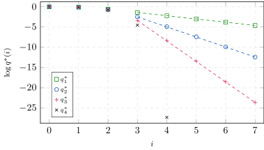
Figure 1: Equilibrium point for $\lambda=0.9$ and distinct limiting outdegree distributions with mean $d=5$: for $q_{1}^{*}$ the limiting outdegree distribution has mass only at $0$ and $2d$, for $q_{2}^{*}$ a uniform distribution on outdegrees between $0$ and $2d$ was used, a Poisson distribution was used for $q_{3}^{*}$ and a deterministic distribution for $q_{4}^{*}$. The tail of $\log q^{*}(i)$ decays almost linearly for the limiting outdegree distributions with mass at zero.

The geometric lower and upper bounds may be intuitively understood as follows. First, observe that tasks leave a server with exactly $i$ tasks at rate $q^{*}(i)-q^{*}(i+1)$ and tasks are dispatched to a server with exactly $i-1$ tasks at a rate that is larger than or equal to $\lambda p(0)\left[q^{*}(i-1)-q^{*}(i)\right]$. In steady state, the departure rate from servers with $i$ tasks must be equal to the rate at which tasks are dispatched to servers with $i-1$ tasks. Thus,

$$q^{*}(i+1) =\sum_{j=i+1}^{\infty}\left[q^{*}(j)-q^{*}(j+1)\right]$$

$$\geq\sum_{j=i+1}^{\infty}\lambda p(0)\left[q^{*}(j-1)-q^{*}(j)\right]=\lambda p(0)q^{*}(i)\geq\left[\lambda p(0)\right]^{i-1}q^{*}(1)=\lambda\left[\lambda p(0)\right]^{i-1}.$$

The geometric upper bound may be explained using a similar heuristic argument, noting that the rate at which tasks are dispatched to servers with exactly $i-1$ tasks is at most $\lambda[1-p(\infty)]\left[q^{*}(i-1)-q^{*}(i)\right]$. Observe here that the probability that an arriving task is diverted away from a busy server is at least $p(\infty)$ since $m=0$ implies that in the limiting regime there are idle servers in the system with probability one.

The geometric decay of the equilibrium occupancy state holds even when the average fraction of isolated servers is arbitrarily small but positive. In other words, to achieve favorable performance, it does not matter so much to have a large average outdegree, but rather to avoid situations where some nodes have outdegree zero. For example, consider a topology with $p(2)=1$ consisting entirely of isolated couples of servers that can forward tasks from one to the other. The decay is substantially faster in this case than in a topology where 1% of the servers cannot forward tasks to other servers and the other 99% of the servers are fully connected; i.e., $p(0)=0.01$ and $p(\infty)=0.99$.

$k$	$R$	$q^{*}(1)$	$q^{*}(2)$	$q^{*}(3)$	$q^{*}(4)$	$q^{*}(5)$	$q^{*}(6)$
$0$	$1.7778$	$0.9000$	$0.5905$	$0.1094$	$0.0001$	$0.0000$	$0.0000$
$1$	$1.7941$	$0.9000$	$0.5927$	$0.1214$	$0.0006$	$0.0000$	$0.0000$
$2$	$1.8528$	$0.9000$	$0.5993$	$0.1603$	$0.0079$	$0.0000$	$0.0000$
$3$	$2.0513$	$0.9000$	$0.6103$	$0.2342$	$0.0712$	$0.0214$	$0.0064$

Table 1: $R$ and $q^{*}(i)$ for $\lambda=0.9$ and limiting outdegree distributions that are uniform in $\{3-k,3,3+k\}$.

5.3 Uniform degrees are beneficial

Corollary 2 gives the limit of the steady-state mean response time of tasks as $n\to\infty$. The value $R$ of this limit is minimal if and only if $q^{*}(i)=0$ for all $i>1$, or equivalently $p(\infty)=1$. Note that this corresponds to a dense limiting regime where the mean outdegree approaches infinity as $n\to\infty$. Indeed, $p(\infty)=1$ implies that for each $k$ there exists $m$ such that $p_{n}(d)<1/2k$ for all $d<k$ and $n\geq m$. This implies that

$$E\left[D_{n}\right]=\sum_{d=0}^{n-1}dp_{n}(d)\geq\sum_{d=k}^{n-1}dp_{n}(d)\geq\frac{k}{2}\quad\text{for all}\quad n\geq m,$$

and since $k$ is arbitrary, we conclude that $E[D_{n}]\to\infty$ as $n\to\infty$ when $p(\infty)=1$

While the steady-state mean response time is theoretically optimal in this dense regime, in practice the communication overhead increases with the average outdegree; because this quantity determines how many neighbors a server needs to poll on average before it can forward a task. As observed in Sections 1 and 2, from a practical perspective it is more relevant to consider the situation where $E[D_{n}]$ is bounded. Below we derive the limiting outdegree distribution $p$ that minimizes the steady-state mean response time $R$ when

$$p(\infty)=0\quad\text{and}\quad\sum_{i=0}^{\infty}ip(i)\leq d$$ (10)

for some given $d\geq 0$; i.e., the mean of the limiting outdegree distribution is at most $d$.

Lemma 4.

Fix $c\in(0,1)$ and suppose that (10) holds. Then

$$\varphi(c)\geq\left(\left\lfloor d\right\rfloor+1-d\right)c^{\left\lfloor d\right\rfloor}+\left(d-\left\lfloor d\right\rfloor\right)c^{\left\lfloor d\right\rfloor+1}\geq c^{d}.$$

Furthermore, $\varphi(c)=c^{d}$ if and only if $d\in\mathbbm{N}$ and $p(d)=1$.

Proof.

Consider the function $f:\mathbbm{R}\longrightarrow\mathbbm{R}$ such that, for all $k\in\mathbbm{Z}$, we have $f(k)=c^{k}$ and the restriction of $f$ to $[k,k+1]$ is linear. Specifically,

$$f(x)\vcentcolon=\left(\left\lfloor x\right\rfloor+1-x\right)c^{\left\lfloor x\right\rfloor}+\left(x-\left\lfloor x\right\rfloor\right)c^{\left\lfloor x\right\rfloor+1}\quad\text{for all}\quad x\in\mathbbm{R}.$$

The convexity of $x\mapsto c^{x}$ implies that $f(x)\geq c^{x}$ for all $x\in\mathbbm{R}$. Moreover,

$$\varphi(c)=\sum_{i=0}^{\infty}p(i)c^{i}=\sum_{i=0}^{\infty}p(i)f(i)\geq f\left(\sum_{i=0}^{\infty}p(i)i\right)\geq f(d)\geq c^{d},$$

since $f$ is convex and decreasing.

Suppose that $p(j)<1$ for some $j$. The strict convexity of $x\mapsto c^{x}$ implies that

$$\varphi(c)=\sum_{i\neq j}p(i)c^{i}+p(j)c^{j}\geq\left[1-p(j)\right]c^{\frac{1}{1-p(j)}\sum_{i\neq j}p(i)i}+p(j)c^{j}>c^{\sum_{i=0}^{\infty}p(i)i}\geq c^{d}.$$

Therefore, it is necessary that $p$ is a deterministic probability measure in order to achieve the lower bound $c^{d}$, and it is straightforward to check that for a deterministic $p$ the lower bound is only attained if $d\in\mathbbm{N}$ and $p(d)=1$. ∎

Proposition 7.

Suppose that (10) holds. Then

$$q^{*}(i)\geq\begin{cases}\lambda^{i}&\text{if}\quad d=0,\\ \lambda^{\frac{(d+1)^{i}-1}{d}}&\text{if}\quad d>0,\end{cases}\quad\text{for all}\quad i\geq 1.$$

If $d\in\mathbbm{N}$ and $p(d)=1$, then we have equality for all $i\geq 1$, and if the latter conditions do not hold, then the inequality is strict for all $i\geq 2$.

Proof.

By Proposition 3 and Lemma 4,

$$q^{*}(i)=\lambda q^{*}(i-1)\varphi\left(q^{*}(i-1)\right)\geq\lambda\left[q^{*}(i-1)\right]^{d+1}\quad\text{for all}\quad i\geq 2.$$

Since $q^{*}(1)=\lambda$, it follows by induction that

$$q^{*}(i)\geq\lambda^{\sum_{j=0}^{i-1}(d+1)^{j}}=\begin{cases}\lambda^{i}&\text{if}\quad d=0,\\ \lambda^{\frac{(d+1)^{i}-1}{d}}&\text{if}\quad d>0,\end{cases}\quad\text{for all}\quad i\geq 1.$$

By Lemma 4, the above inequality is strict for all $i\geq 2$ unless $d\in\mathbbm{N}$ and $p(d)=1$, which results in equality for all $i\geq 1$. ∎

Under the sparsity constraint (10), the equilibrium $q^{*}$ is minimized coordinatewise if and only if $d\in\mathbbm{N}$ and the limiting outdegree distribution is deterministic with $p(d)=1$. In particular, the minimum value of $R$ is only attained for this limiting outdegree distribution and the fraction of servers with at least $i$ tasks is minimal for each $i$. Also, the numerical results in Figure 1 and Table 1 suggest that $q^{*}$ decreases coordinatewise as the limiting outdegree distribution becomes more concentrated around $d$.

Remark 7.

The lower bound in Proposition 7 is only tight when $d\in\mathbbm{N}$, but it is possible to derive a lower bound that is tight also when $d\notin\mathbbm{N}$. This lower bound is obtained in a similar fashion but invoking the inequality $\varphi(c)\geq\left(\left\lfloor d\right\rfloor+1-d\right)c^{\left\lfloor d\right\rfloor}+\left(d-\left\lfloor d\right\rfloor\right)c^{\left\lfloor d\right\rfloor+1}$ instead of the inequality $\varphi(c)\geq c^{d}$, which is only tight for $d\in\mathbbm{N}$. However, this more refined lower bound is rather unwieldy.

6 Proof of the fluid limit

In this section we prove Theorem 1. As a first step, we define the processes $\left\{\boldsymbol{q}_{n}:n\geq 1\right\}$ and $\left\{\boldsymbol{X}_{n}:n\geq 1\right\}$ as deterministic functions of the following stochastic primitives.

1. Driving Poisson processes: independent Poisson processes $\mathcal{N}^{a}$ and $\left\{\mathcal{N}_{i}^{d}:i\geq 1\right\}$ of unit intensity, for counting the arrivals and departures of tasks, respectively.

2. Selection variables: independent random variables $\left\{u_{n}^{m},U_{i,n}^{m}:i,m,n\geq 1\right\}$ such that $u_{n}^{m}$ is uniform in $V_{n}$ and $U_{i,n}^{m}$ is uniform in $[0,1)$ for all $m$ and $n$.

3. Initial conditions: a sequence $\left\{X_{n}:n\geq 1\right\}$ of random vectors describing the initial number of tasks at each server and such that the corresponding sequence of occupancy states $\left\{q_{n}:n\geq 1\right\}$ is tight in $\ell_{1}$.

4. Random graphs: independent random graphs $\left\{G_{n}^{m}:m\geq 0,n\geq 1\right\}$ such that for each fixed $n$ all the graphs $\left\{G_{n}^{m}:m\geq 0\right\}$ have node set $V_{n}$ and a common distribution that satisfies Assumption 1 and is invariant under permutations of the nodes.

5. Resampling processes: càdlàg processes $\left\{\mathcal{R}_{n}:n\geq 1\right\}$ satisfying Assumption 1.

The sample paths of $\boldsymbol{q}_{n}$ and $\boldsymbol{X}_{n}$ are constructed on the completion of the product of the probability spaces where the stochastic primitives are defined. This construction is such that certain stochastic equations hold, as we explain in the following section.

6.1 Stochastic equations

For each fixed $n$, the times at which the graph is sampled are $\sigma_{n}^{0}\vcentcolon=0$ and the jump times $\left\{\sigma_{n}^{m}:m\geq 1\right\}$ of the resampling process $\mathcal{R}_{n}$. Specifically,

$$\boldsymbol{G}_{n}(t)=G_{n}^{0}\quad\text{if}\quad\sigma_{n}^{0}\leq t\leq\sigma_{n}^{1}\quad\text{and}\quad\boldsymbol{G}_{n}(t)=G_{n}^{m}\quad\text{if}\quad\sigma_{n}^{m}<t\leq\sigma_{n}^{m+1}.$$

In addition, tasks arrive at the jump times $\left\{\tau_{n}^{m}:m\geq 1\right\}$ of the arrival process $\mathcal{N}_{n}^{a}$ defined by $\mathcal{N}_{n}^{a}(t)\vcentcolon=\mathcal{N}^{a}(\lambda_{n}t)$. At time $\tau_{n}^{m}$, a task appears at server $u_{n}^{m}$ and we let

$$I_{n}^{m}(X,i)\vcentcolon=\mathbbm{1}_{\left\{\min\left\{X(v):v=u_{n}^{m}\ \text{or}\ \left(u_{n}^{m},v\right)\in\boldsymbol{E}_{n}\left(\tau_{n}^{m-}\right)\right\}\geq i\right\}}\quad\text{for all}\quad X\in\mathbbm{N}^{n}.$$

If $X(v)$ represents the number of tasks at server $v$ right before $\tau_{n}^{m}$, then $I_{n}^{m}(X,i)=1$ if and only if the task arriving at time $\tau_{n}^{m}$ is dispatched to a server with at least $i$ tasks.

The processes $\boldsymbol{q}_{n}$ and $\boldsymbol{X}_{n}$ are constructed in Appendix C as deterministic functions of the stochastic primitives within a set of probability one. Both are piecewise constant càdlàg processes defined on $[0,\infty)$ and have jumps of size $1/n$ and jumps of unit size, respectively. Moreover, the following stochastic equations hold:

$$\begin{split}\boldsymbol{q}_{n}(t,i)&=\boldsymbol{q}_{n}(0,i)+\frac{1}{n}\sum_{m=1}^{\mathcal{N}_{n}^{a}(t)}\left[I_{n}^{m}\left(\boldsymbol{X}_{n}\left(\tau_{n}^{m-}\right),i-1\right)-I_{n}^{m}\left(\boldsymbol{X}_{n}\left(\tau_{n}^{m-}\right),i\right)\right]\\ &-\frac{1}{n}\mathcal{N}_{i}^{d}\left(n\int_{0}^{t}\left[\boldsymbol{q}_{n}(s,i)-\boldsymbol{q}_{n}(s,i+1)\right]ds\right)\end{split}$$ (11)

for all $i\geq 1$ and $t\geq 0$ with probability one. Indeed, the first term on the right is the initial occupancy state, the second term counts the arrivals to servers with exactly $i-1$ tasks and the third term counts the departures from servers with exactly $i$ tasks.

6.2 Decomposition of the equations

Consider the function defined by

$$\alpha_{n}(d,x)\vcentcolon=\begin{cases}\prod_{m=0}^{d-1}\left(\frac{nx-m}{n-m}\right)^{+}&\text{if}\quad d\leq n,\\ 0&\text{if}\quad d>n,\end{cases}\quad\text{for all}\quad x\in[0,1].$$ (12)

If $nx\in\mathbbm{N}$ and a subset of $\{1,\dots,n\}$ consisting of $d\leq n$ elements is drawn uniformly at random, then $\alpha_{n}(d,x)$ is the probability that this subset is contained in $\{1,\dots,nx\}$.

Suppose that the fraction of servers with at least $i$ tasks is $x$ when a task arrives. The server $u$ that initially receives the task is uniformly random and thus has outdegree $d$ with probability $p_{n}(d)$. Furthermore, given that the outdegree of $u$ is $d$, the probability that all the servers in the neighborhood of $u$ have at least $i$ tasks is $\alpha_{n}(d+1,x)$ because the distribution of the graph is invariant under permutations of the nodes. Hence, the probability that the task is dispatched to a server with at least $i$ tasks is

$$\beta_{n}(x)\vcentcolon=\sum_{d=0}^{n-1}\alpha_{n}\left(d+1,x\right)p_{n}(d)\quad\text{for all}\quad x\in[0,1].$$ (13)

In particular, we have

$$E\left[I_{n}^{m}(X,i)\right]=\beta_{n}\left(q(i)\right)\quad\text{for all}\quad X\in\mathbbm{N}^{n}\quad\text{and}\quad q(i)\vcentcolon=\frac{1}{n}\sum_{u=1}^{n}\mathbbm{1}_{\left\{X(u)\geq 1\right\}}.$$ (14)

The expectation is taken with respect to the stochastic primitives, or more precisely just with respect to the graph right before $\tau_{n}^{m}$ and the server $u_{n}^{m}$ at which the task originally appears; indeed, note that $I_{n}^{m}(X,i)$ only depends on these two random variables.

Remark 8.

The above arguments break down if the graph at the time of the arrival is given. In that case the probability that a task is dispatched to a server with at least $i$ tasks depends on the given graph and the number of tasks at each individual server.

Consider the processes defined by

$$\begin{split}\bar{\boldsymbol{q}}_{n}(t)\vcentcolon=\sum_{m=0}^{\infty}\boldsymbol{q}_{n}\left(\sigma_{n}^{m}\right)\mathbbm{1}_{\left\{\sigma_{n}^{m}\leq t<\sigma_{n}^{m+1}\right\}}\quad\text{and}\quad\bar{\boldsymbol{X}}_{n}(t)\vcentcolon=\sum_{m=0}^{\infty}\boldsymbol{X}_{n}\left(\sigma_{n}^{m}\right)\mathbbm{1}_{\left\{\sigma_{n}^{m}\leq t<\sigma_{n}^{m+1}\right\}},\end{split}$$

which correspond to sampling the state of the system at the resampling times. Also, let

$$q_{n}^{m}\vcentcolon=\boldsymbol{q}_{n}\left(\tau_{n}^{m-}\right),\quad\bar{q}_{n}^{m}\vcentcolon=\bar{\boldsymbol{q}}_{n}\left(\tau_{n}^{m-}\right),\quad X_{n}^{m}\vcentcolon=\boldsymbol{X}_{n}\left(\tau_{n}^{m-}\right)\quad\text{and}\quad\bar{X}_{n}^{m}\vcentcolon=\bar{\boldsymbol{X}}_{n}\left(\tau_{n}^{m-}\right).$$

We define processes $\boldsymbol{L}_{n}$, $\boldsymbol{M}_{n}$ and $\boldsymbol{u}_{n}$ as follows. If at most one task arrives between any two successive resampling times, then we say that $\mathcal{R}_{n}$ separates arrivals fully and we let

$$\begin{split}&\boldsymbol{L}_{n}(t,i)\vcentcolon=0,\\ &\boldsymbol{M}_{n}(t,i)\vcentcolon=\frac{1}{n}\sum_{m=1}^{\mathcal{N}_{n}^{a}(t)}\left[I_{n}^{m}\left(X_{n}^{m},i\right)-\beta_{n}\left(q_{n}^{m}(i)\right)\right],\\ &\boldsymbol{u}_{n}(t,i)\vcentcolon=\frac{1}{n}\sum_{m=1}^{\mathcal{N}_{n}^{a}(t)}\beta_{n}\left(q_{n}^{m}(i)\right),\end{split}$$ (15)

for all $i\geq 0$ and $t\geq 0$. If $\mathcal{R}_{n}$ does not separate arrivals fully, then we define

$$\begin{split}&\boldsymbol{L}_{n}(t,i)\vcentcolon=\frac{1}{n}\sum_{m=1}^{\mathcal{N}_{n}^{a}(t)}\left[I_{n}^{m}\left(X_{n}^{m},i\right)-I_{n}^{m}\left(\bar{X}_{n}^{m},i\right)\right],\\ &\boldsymbol{M}_{n}(t,i)\vcentcolon=\frac{1}{n}\sum_{m=1}^{\mathcal{N}_{n}^{a}(t)}\left[I_{n}^{m}\left(\bar{X}_{n}^{m},i\right)-\beta_{n}\left(\bar{q}_{n}^{m}(i)\right)\right],\\ &\boldsymbol{u}_{n}(t,i)\vcentcolon=\frac{1}{n}\sum_{m=1}^{\mathcal{N}_{n}^{a}(t)}\beta_{n}\left(\bar{q}_{n}^{m}(i)\right).\end{split}$$ (16)

Note that $X_{n}^{m}$ and $q_{n}^{m}$ have been replaced by $\bar{X}_{n}^{m}$ and $\bar{q}_{n}^{m}$ in the definitions of $\boldsymbol{M}_{n}$ and $\boldsymbol{u}_{n}$ provided in (16). Also, the sum of the three processes is the same under (15) and (16).

Remark 9.

If the resampling process separates arrivals fully, then the graph is resampled between any two consecutive arrival times. The definitions provided in (15) significantly simplify the proof of the fluid limit when all the resampling processes $\mathcal{R}_{n}$ separate arrivals fully. But this simplification is no longer possible when successive arrivals have a positive probability of being dispatched using the same graph. In this case we must resort to (16).

The stochastic equations (11) can now be expressed as follows:

$$\boldsymbol{q}_{n}=\boldsymbol{q}_{n}(0)+\boldsymbol{v}_{n}+\boldsymbol{w}_{n},$$ (17)

where for all $i\geq 1$ and $t\geq 0$, the vanishing process $\boldsymbol{v}_{n}$ is defined by

$$\begin{split}\boldsymbol{v}_{n}(t,i)&\vcentcolon=\boldsymbol{L}_{n}(t,i-1)-\boldsymbol{L}_{n}(t,i)+\boldsymbol{M}_{n}(t,i-1)-\boldsymbol{M}_{n}(t,i)\\ &+\int_{0}^{t}\left[\boldsymbol{q}_{n}(s,i)-\boldsymbol{q}_{n}(s,i+1)\right]ds-\frac{1}{n}\mathcal{N}_{i}^{d}\left(n\int_{0}^{t}\left[\boldsymbol{q}_{n}(s,i)-\boldsymbol{q}_{n}(s,i+1)\right]ds\right),\end{split}$$ (18)

and the drift process $\boldsymbol{w}_{n}$ is defined by

$$\begin{split}\boldsymbol{w}_{n}(t,i)\vcentcolon=\boldsymbol{u}_{n}(t,i-1)-\boldsymbol{u}_{n}(t,i)-\int_{0}^{t}\left[\boldsymbol{q}_{n}(s,i)-\boldsymbol{q}_{n}(s,i+1)\right]ds.\end{split}$$ (19)

The road map for proving Theorem 1 is as follows. In Section 6.3 we formally define the pseudo-separation property mentioned in Assumption 1 and we prove Proposition 1. In Section 6.4 we show that $\boldsymbol{v}_{n}\Rightarrow 0$ as $n\to\infty$ with respect to a suitable topology. Informally, this implies that the asymptotic behavior of $\boldsymbol{q}_{n}$ is essentially captured by (19) in the limit as $n\to\infty$. Then we prove in Section 6.5 that $\left\{\boldsymbol{q}_{n}:n\geq 1\right\}$ is tight in $D_{\ell_{1}}[0,\infty)$. This implies that every subsequence of $\left\{\boldsymbol{q}_{n}:n\geq 1\right\}$ has a further subsequence that converges weakly in $D_{\ell_{1}}[0,\infty)$ to some process $\boldsymbol{q}$. Finally, (19) is used to establish that the limit $\boldsymbol{q}$ of any convergent subsequence satisfies (4) almost surely. Essentially, the first two terms of (19) yield the first term of (4) and the last term of (19) gives the last term of (4).

6.3 Pseudo-separation property

Below we define the pseudo-separation property mentioned in Assumption 1. This property applies to sequences of resampling processes $\mathcal{R}_{n}$ and concerns the asymptotic behavior of the processes as $n\to\infty$. In contrast, the property of separating arrivals fully applies to individual resampling processes $\mathcal{R}_{n}$; i.e., the number of servers $n$ is fixed.

Definition 1.

The resampling process $\mathcal{R}_{n}$ is said to separate arrivals fully if at most one task arrives between any two successive resampling times with probability one. Consider the following random variables:

$$\begin{split}&\Delta_{n}(T)\vcentcolon=\sup\left\{t-\sigma_{n}^{m}:m\leq\mathcal{R}_{n}(T)\ \text{and}\ \sigma_{n}^{m}\leq t\leq\min\left\{\sigma_{n}^{m+1},T\right\}\right\},\\ &\Sigma_{n}(T)\vcentcolon=\sum_{m=1}^{\mathcal{R}_{n}(T)+1}\frac{1}{n^{2}}\left[\left(d_{n}^{-}+1\right)\left(A_{n}^{m}+D_{n}^{m}-1\right)A_{n}^{m}+\left(A_{n}^{m}\right)^{2}\right],\end{split}$$

where $A_{n}^{m}$ and $D_{n}^{m}$ are the number of arrivals and departures in $\left(\sigma_{n}^{m-1},\sigma_{n}^{m}\right]$, respectively. Also, let $\mathcal{K}$ be the set of indexes $k$ such that $\mathcal{R}_{k}$ does not separate arrivals fully. The resampling processes $\left\{\mathcal{R}_{n}:n\geq 1\right\}$ are said to pseudo-separate events if $\mathcal{K}$ is finite or $\mathcal{K}$ is infinite and the following limits hold:

$$\Delta_{k}(T)\Rightarrow 0\quad\text{as}\quad k\to\infty\quad\text{and}\quad\lim_{k\to\infty}E\left[\Sigma_{k}(T)\right]=0\quad\text{for all}\quad T\geq 0,$$ (20)

where both limits are taken over the indexes $k\in\mathcal{K}$.

It is possible that all the resampling processes $\mathcal{R}_{n}$ separate arrivals fully and $E\left[\Sigma_{n}(T)\right]$ does not approach zero with $n$ for any $T\geq 0$. For example, if the resampling times coincide with the arrival times, then $A_{n}^{m}=1$ and $E\left[D_{n}^{m}\right]$ is of order $n\left(\sigma_{n}^{m}-\sigma_{n}^{m-1}\right)$. Therefore,

$$E\left[\Sigma_{n}(T)\right]\geq E\left[\sum_{m=1}^{\mathcal{R}_{n}(T)+1}\frac{\left(d_{n}^{-}+1\right)D_{n}^{m}}{n^{2}}\right]$$

is lower bounded by a quantity of order $\left(d_{n}^{-}+1\right)T/n$, which does not approach zero as $n\to\infty$ if $d_{n}^{-}/n\nrightarrow 0$. However, Theorem 1 covers sequences of resampling processes such that $\mathcal{R}_{n}$ separates arrivals fully for infinitely many $n$. For this reason we require that (20) holds only for the subsequence of processes that do not separate arrivals fully.

The next lemma gathers some useful properties of the random variables $A_{n}^{m}$ and $D_{n}^{m}$, and will be used to prove Proposition 1; we prove the lemma in Appendix B.

Lemma 5.

Let $A_{n}^{m}$ denote the number of tasks that arrive in $\left(\sigma_{n}^{m-1},\sigma_{n}^{m}\right]$, let $D_{n}^{m}$ be the number of tasks that depart and let $\mathcal{H}_{n}\vcentcolon=\sigma\left(\mathcal{R}_{n}(t):t\geq 0\right)$ be the $\sigma$-algebra generated by the resampling times. If the resampling process is independent of the arrival times of tasks or is independent of the departure times of tasks, then

$$E\left[A_{n}^{m}\nonscript\;\middle|\nonscript\;\mathcal{H}_{n}\right]=\mathrm{Var}\left[A_{n}^{m}\nonscript\;\middle|\nonscript\;\mathcal{H}_{n}\right]=\lambda_{n}\left(\sigma_{n}^{m}-\sigma_{n}^{m-1}\right)\quad\text{and}\quad E\left[D_{n}^{m}\nonscript\;\middle|\nonscript\;\mathcal{H}_{n}\right]\leq n\left(\sigma_{n}^{m}-\sigma_{n}^{m-1}\right),$$

respectively. If condition (c) of Proposition 1 holds, then

$$\lim_{n\to\infty}\mu_{n}E\left[\sum_{m=1}^{\mathcal{R}_{n}(t)+1}\left(\sigma_{n}^{m}-\sigma_{n}^{m-1}\right)^{2}\right]=E\left[\left(\sigma_{1}^{1}\right)^{2}\right]t\quad\text{for all}\quad t\geq 0.$$ (21)

We now prove Proposition 1.

Proof of Proposition 1.

In order to prove that $\left\{\mathcal{R}_{n}:n\geq 1\right\}$ pseudo-separates events, we must show that the limits in (20) hold when we only consider the indexes $n$ such that the resampling process does not separate arrivals fully. Hence, we may assume without loss of generality that the resampling process $\mathcal{R}_{n}$ does not separate arrivals fully for any $n$; i.e., if (a) holds, then we assume that $\kappa_{n}\geq 1$ for all $n$.

Let us fix an arbitrary $T\geq 0$. First we establish that $\Delta_{n}(T)\Rightarrow 0$ as $n\to\infty$ when any of the conditions stated in the proposition holds. The latter limit clearly holds when (b) holds, which implies that $\Delta_{n}(T)\leq 1/\mu_{n}$. If condition (a) holds instead, then

$$\kappa_{n}+1\geq\left|\mathcal{N}_{n}^{a}\left(t\right)-\mathcal{N}_{n}^{a}\left(\sigma_{n}^{m}\right)\right|\geq\lambda_{n}\left|t-\sigma_{n}^{m}\right|-2\sup_{u\in[0,T]}\left|\mathcal{N}_{n}^{a}(u)-\lambda_{n}u\right|$$

for all $m\leq\mathcal{R}_{n}(T)$ and $\sigma_{n}^{m}\leq t\leq\min\left\{\sigma_{n}^{m+1},T\right\}$. It follows that

$$\Delta_{n}(T)\leq\frac{\kappa_{n}+1}{\lambda_{n}}+\frac{2}{\lambda_{n}}\sup_{u\in[0,T]}\left|\mathcal{N}_{n}^{a}(u)-\lambda_{n}u\right|.$$ (22)

The right-hand side goes to zero in probability by (3) and the law of large numbers for the Poisson process, hence $\Delta_{n}(T)\Rightarrow 0$ as $n\to\infty$ also in this case. A similar argument applies when condition (c) holds. Indeed, note that

$$1\geq\left|\mathcal{R}_{n}(t)-\mathcal{R}_{n}\left(\sigma_{n}^{m}\right)\right|\geq\mu_{n}\left|t-\sigma_{n}^{m}\right|-2\sup_{u\in[0,T]}\left|\mathcal{R}_{n}(u)-\mu_{n}u\right|$$

for all $m\leq\mathcal{R}_{n}(T)$ and $\sigma_{n}^{m}\leq t\leq\min\left\{\sigma_{n}^{m+1},T\right\}$. Arguing as above, we conclude from the law of large numbers for the renewal process $\mathcal{R}$ that $\Delta_{n}(T)\Rightarrow 0$ as $n\to\infty$.

We now prove that $E\left[\Sigma_{n}(T)\right]\to 0$ as $n\to\infty$. For this purpose we first note that

$$E\left[\Sigma_{n}(T)\right]=\frac{1}{n^{2}}E\left[\sum_{m=1}^{\mathcal{R}_{n}(T)+1}E\left[\left(d_{n}^{-}+1\right)\left(A_{n}^{m}+D_{n}^{m}-1\right)A_{n}^{m}+\left(A_{n}^{m}\right)^{2}\nonscript\;\middle|\nonscript\;\mathcal{H}_{n}\right]\right],$$

where $\mathcal{H}_{n}\vcentcolon=\sigma\left(\mathcal{R}_{n}(t):t\geq 0\right)$ is the $\sigma$-algebra generated by the resampling times. Let

$$Y_{n}^{m}\vcentcolon=\left(d_{n}^{-}+1\right)\left(E\left[A_{n}^{m}\left(A_{n}^{m}-1\right)\nonscript\;\middle|\nonscript\;\mathcal{H}_{n}\right]+E\left[A_{n}^{m}\nonscript\;\middle|\nonscript\;\mathcal{H}_{n}\right]E\left[D_{n}^{m}\nonscript\;\middle|\nonscript\;\mathcal{H}_{n}\right]\right)+E\left[\left(A_{n}^{m}\right)^{2}\nonscript\;\middle|\nonscript\;\mathcal{H}_{n}\right]$$

denote term $m$ in the above summation. Then we may write

$$E\left[\Sigma_{n}(T)\right]\leq\frac{1}{n^{2}}E\left[\sum_{m=1}^{\mathcal{R}_{n}(T)}Y_{n}^{m}\right]+\frac{1}{n^{2}}E\left[Y_{n}^{\mathcal{R}_{n}(T)+1}\right].$$

Next we prove that the first term on the right-hand side approaches zero as $n\to\infty$, and it is straightforward to check that the second term also vanishes; considering the sum of $Y_{n}^{m}$ over $m=1,\dots,\mathcal{R}_{n}(T)$ instead of $m=1,\dots,\mathcal{R}_{n}(T)+1$ simplifies calculations.

If (a) holds, then Lemma 5 yields

$$Y_{n}^{m}\leq\left(d_{n}^{-}+1\right)\left[\left(\kappa_{n}+1\right)\kappa_{n}+(\kappa_{n}+1)n\left(\sigma_{n}^{m}-\sigma_{n}^{m-1}\right)\right]+\left(\kappa_{n}+1\right)^{2}.$$

Moreover, $E\left[\mathcal{R}_{n}(T)\right]\leq\lambda_{n}T/\left(\kappa_{n}+1\right)$ and thus

$$\frac{1}{n^{2}}E\left[\sum_{m=1}^{\mathcal{R}_{n}(T)}Y_{n}^{m}\right]\leq\frac{\left(d_{n}^{-}+1\right)\left[\kappa_{n}\lambda_{n}T+\left(\kappa_{n}+1\right)nT\right]+\left(\kappa_{n}+1\right)\lambda_{n}T}{n^{2}}.$$

If $\kappa_{n}\geq 1$ for all $n$, then the right-hand side approaches zero as $n\to\infty$ by (3).

Suppose now that conditions (b) or (c) hold. Lemma 5 implies that

$$Y_{n}^{m}\leq\left(d_{n}^{-}+1\right)\left(\lambda_{n}^{2}+\lambda_{n}n\right)\left(\sigma_{n}^{m}-\sigma_{n}^{m-1}\right)^{2}+\lambda_{n}\left(\sigma_{n}^{m}-\sigma_{n}^{m-1}\right)+\lambda_{n}^{2}\left(\sigma_{n}^{m}-\sigma_{n}^{m-1}\right)^{2}.$$

If (b) holds, then $\sigma_{n}^{m}-\sigma_{n}^{m-1}\leq 1/\mu_{n}$ and $\left(\sigma_{n}^{m}-\sigma_{n}^{m-1}\right)^{2}\leq\left(\sigma_{n}^{m}-\sigma_{n}^{m-1}\right)/\mu_{n}$. Therefore,

$$\frac{1}{n^{2}}E\left[\sum_{m=1}^{\mathcal{R}_{n}(T)}Y_{n}^{m}\right]\leq\frac{\left(d_{n}^{-}+1\right)\left(\lambda_{n}^{2}+\lambda_{n}n\right)T+\lambda_{n}^{2}T}{\mu_{n}n^{2}}+\frac{\lambda_{n}T}{n^{2}}.$$

It follows from (3) that the right-hand side vanishes as $n\to\infty$. Finally, if (c) holds, then

$$\frac{1}{n^{2}}E\left[\sum_{m=1}^{\mathcal{R}_{n}(T)}Y_{n}^{m}\right]\leq\frac{\left(d_{n}^{-}+1\right)\left(\lambda_{n}^{2}+\lambda_{n}n\right)+\lambda_{n}^{2}}{n^{2}}E\left[\sum_{m=1}^{\mathcal{R}_{n}(t)+1}\left(\sigma_{n}^{m}-\sigma_{n}^{m-1}\right)^{2}\right]+\frac{\lambda_{n}T}{n^{2}},$$

and the right-hand side approaches zero as $n\to\infty$ by (3) and (21). ∎

The next corollary says that if $\left\{\mathcal{R}_{n}:n\geq 1\right\}$ pseudo-separates events, then $\Delta_{n}(T)\Rightarrow 0$ as $n\to\infty$ for all $T\geq 0$. In other words, this means that the limit holds without considering only the resampling processes that do not separate arrivals fully.

Corollary 3.

If $\left\{\mathcal{R}_{n}:n\geq 1\right\}$ pseudo-separates events, then

$$\Delta_{n}(T)\Rightarrow 0\quad\text{as}\quad n\to\infty\quad\text{for all}\quad T\geq 0.$$

Proof.

Note that (22) with $\kappa_{n}=0$ holds when $\mathcal{R}_{n}$ separates arrivals fully. ∎

6.4 Vanishing processes

Endow $\mathbbm{R}^{\mathbbm{N}}$ with the metric

$$d(x,y)\vcentcolon=\sum_{i=0}^{\infty}\frac{\min\left\{|x(i)-y(i)|,1\right\}}{2^{i}}\quad\text{for all}\quad x,y\in\mathbbm{R}^{\mathbbm{N}},$$

which is compatible with the product topology. Also, let $D_{\mathbbm{R}^{\mathbbm{N}}}[0,\infty)$ be the space of càdlàg functions from $[0,\infty)$ into $\mathbbm{R}^{\mathbbm{N}}$ with the topology of uniform convergence over compact sets. In this section we establish that $\boldsymbol{v}_{n}\Rightarrow 0$ in $D_{\mathbbm{R}^{\mathbbm{N}}}[0,\infty)$ as $n\to\infty$.

For this purpose, let $D_{\mathbbm{R}}[0,T]$ be the space of real càdlàg functions defined on $[0,T]$, which we endow with the uniform norm, defined by

$$\left|\left|\boldsymbol{x}\right|\right|_{T}\vcentcolon=\sup_{t\in[0,T]}|\boldsymbol{x}(t)|\quad\text{for all}\quad\boldsymbol{x}\in D_{\mathbbm{R}}[0,T].$$

The following lemma is proved in Appendix B.

Lemma 6.

Suppose that $\left\{\boldsymbol{x}_{n}:n\geq 1\right\}$ are random variables with values in $D_{\mathbbm{R}^{\mathbbm{N}}}[0,\infty)$. The following properties are equivalent.

1. $\boldsymbol{x}_{n}\Rightarrow 0$ in $D_{\mathbbm{R}^{\mathbbm{N}}}[0,\infty)$ as $n\to\infty$.

2. $\boldsymbol{x}_{n}(i)\Rightarrow 0$ in $D_{\mathbbm{R}}[0,T]$ as $n\to\infty$ for all $i\geq 0$ and $T\geq 0$.

By Lemma 6, we can prove that $\boldsymbol{v}_{n}\Rightarrow 0$ in $D_{\mathbbm{R}^{\mathbbm{N}}}[0,\infty)$ by showing that $\boldsymbol{v}_{n}(i)\Rightarrow 0$ in $D_{\mathbbm{R}}[0,T]$ for all $i\geq 0$ and $T\geq 0$. We prove this by showing that the first four terms and the difference between the last two terms on the right-hand side of (18) converge to zero in probability. In the next two sections we show that $\boldsymbol{L}_{n}(i)\Rightarrow 0$ and $\boldsymbol{M}_{n}(i)\Rightarrow 0$ in $D_{\mathbbm{R}}[0,T]$ for all $i\geq 0$ and $T\geq 0$. Then we invoke the law of large numbers for the Poisson process to prove that the difference between the last two terms of (18) also converges to zero.

6.4.1 Limit of the processes $\boldsymbol{L}_{n}$

For each $t\geq 0$, we define

$$K_{n}(t)\vcentcolon=\left\{u\in V_{n}:\boldsymbol{X}_{n}(t,v)=\bar{\boldsymbol{X}}_{n}(t,v)\ \text{if}\ v=u\ \text{or}\ (u,v)\in\boldsymbol{E}_{n}(t)\right\}.$$

Note that all the servers in the neighborhood of a server $u\in K_{n}(t)$ have the same number of tasks as they had at the last resampling time. Hence,

$$\left|I_{n}^{m}\left(X_{n}^{m},i\right)-I_{n}^{m}(\bar{X}_{n}^{m},i)\right|\leq\mathbbm{1}_{\left\{u_{n}^{m}\notin K_{n}\left(\tau_{n}^{m-}\right)\right\}}\quad\text{for all}\quad i\geq 0\quad\text{and}\quad m\geq 1,$$

where we recall that $u_{n}^{m}$ is the server where a task appears at time $\tau_{n}^{m}$.

Remark 10.

If a task appears in the complement $K_{n}^{c}(t)$ of $K_{n}(t)$, then the dispatching decision is influenced by a server that experienced an arrival or departure between time $t$ and the preceding resampling time. The set $K_{n}^{c}(t)$ is reminiscent of the influence process introduced in the proof of [8, Proposition 7.1]; the setup considered there is a system of parallel single-server queues where the classical power-of-$d$ policy is used to balance the load. The influence process of a server $u$ describes the set of servers that influence the queue length of $u$ over $[0,t]$. This process is used in [8] to prove that a fixed and finite set of queue lengths observed at a fixed time $t$ become asymptotically independent and identically distributed as the number of servers approaches infinity, provided that all the queue lengths in the system are independent and identically distributed at time zero. The proof relies on approximating the number of servers in the influence process of a single server by a continuous-time branching process where each parent has $d$ children. However, the present paper uses the sets $K_{n}^{c}(t)$ to show that $\left|\left|\boldsymbol{L}_{n}(i)\right|\right|_{T}$ converges in probability to zero. For this purpose we provide a bound for the size of the set $K_{n}^{c}(t)$. The bound increases linearly with the number of arrivals since the preceding resampling time, as in a continuous-time branching process, but depends on the number of departures as well.

Let $A_{n}^{m}$ denote the number of tasks that arrive in $\left(\sigma_{n}^{m-1},\sigma_{n}^{m}\right]$ and let $D_{n}^{m}$ denote the number of tasks that depart. If $\sigma_{n}^{m-1}<t\leq\sigma_{n}^{m}$ and $k$ tasks arrive in $\left(\sigma_{n}^{m-1},t\right]$, then at time $t$ at most $k+D_{n}^{m}$ servers have a number of tasks that is different from the number of tasks that they had at time $\sigma_{n}^{m-1}$. Since each of these servers can be in the neighborhood of at most $d_{n}^{-}$ servers, it follows that at most $\left(k+D_{n}^{m}\right)\left(d_{n}^{-}+1\right)$ servers are not in $K_{n}(t)$. Thus, the random variables $A_{n}^{m}$ and $D_{n}^{m}$ can be used to upper bound $\left|\left|\boldsymbol{L}_{n}(i)\right|\right|_{T}$ for all $i\geq 0$ and $T\geq 0$. This observation is used in the following proposition.

Proposition 8.

We have

$$\boldsymbol{L}_{n}(i)\Rightarrow 0\quad\text{in}\quad D_{\mathbbm{R}}[0,T]\quad\text{as}\quad n\to\infty\quad\text{for all}\quad i\geq 0\quad\text{and}\quad T\geq 0,$$

and in particular $\boldsymbol{L}_{n}\Rightarrow 0$ in $D_{\mathbbm{R}^{\mathbbm{N}}}[0,\infty)$ as $n\to\infty$.

Proof.

We must prove that

$$\lim_{n\to\infty}P\left(\left|\left|\boldsymbol{L}_{n}(i)\right|\right|_{T}\geq\varepsilon\right)=0\quad\text{for all}\quad\varepsilon>0,\quad i\geq 0\quad\text{and}\quad T\geq 0.$$

For this purpose, let us fix $\varepsilon>0$, $i\geq 0$ and $T\geq 0$, and note that

$$\left|\left|\boldsymbol{L}_{n}(i)\right|\right|_{T}\leq\frac{1}{n}\sum_{m=1}^{\mathcal{N}_{n}^{a}(T)}\left|I_{n}^{m}\left(X_{n}^{m},i\right)-I_{n}^{m}\left(\bar{X}_{n}^{m},i\right)\right|\leq\frac{1}{n}\sum_{m=1}^{\mathcal{N}_{n}^{a}(T)}\mathbbm{1}_{\left\{u_{n}^{m}\notin K_{n}\left(\tau_{n}^{m-}\right)\right\}}.$$

By Markov’s inequality, we may focus on bounding the expectation of the right-hand side:

$$P\left(\left|\left|\boldsymbol{L}_{n}(i)\right|\right|_{T}\geq\varepsilon\right)\leq P\left(\frac{1}{n}\sum_{m=1}^{\mathcal{N}_{n}^{a}(T)}\mathbbm{1}_{\left\{u_{n}^{m}\notin K_{n}\left(\tau_{n}^{m-}\right)\right\}}\geq\varepsilon\right)\leq\frac{1}{n\varepsilon}E\left[\sum_{m=1}^{\mathcal{N}_{n}^{a}(T)}\mathbbm{1}_{\left\{u_{n}^{m}\notin K_{n}\left(\tau_{n}^{m-}\right)\right\}}\right].$$

Let $A_{n}^{l}$ and $D_{n}^{l}$ be the number of arrivals and departures in $\left(\sigma_{n}^{l-1},\sigma_{n}^{l}\right]$, respectively, and suppose that $\tau_{n}^{m}<\tau_{n}^{m+1}<\dots<\tau_{n}^{m+A_{n}^{l}-1}$ are all the arrival times in this interval. Then

$$\left|K_{n}^{c}\left(\tau_{n}^{m+k-}\right)\right|\leq\left(k+D_{n}^{l}\right)\left(d_{n}^{-}+1\right)\quad\text{for all}\quad 0\leq k\leq A_{n}^{l}-1,$$

where $K_{n}^{c}(t)$ denotes the complement of $K_{n}(t)$. Recall that this holds since the number of tasks may have changed in at most $k+D_{n}^{l}$ servers between $\sigma_{n}^{l-1}$ and right before $\tau_{n}^{m+k}$, and each server can be in the neighborhood of at most $d_{n}^{-}$ other servers.

Let $\mathcal{G}_{n}\vcentcolon=\sigma\left(\mathcal{N}_{n}^{a}(t),\mathcal{R}_{n}(t):t\geq 0\right)$ denote the $\sigma$-algebra generated by the arrival and resampling times. Since $u_{n}^{m}$ is uniformly distributed in $V_{n}$, the above observation about the sets $K_{n}^{c}\left(\tau_{n}^{m-}\right)$ implies that

$$\frac{1}{n}E\left[\sum_{m=1}^{\mathcal{N}_{n}^{a}(T)}\mathbbm{1}_{\left\{u_{n}^{m}\notin K_{n}\left(\tau_{n}^{m-}\right)\right\}}\right] =\frac{1}{n}E\left[\sum_{m=1}^{\mathcal{N}_{n}^{a}(T)}E\left[\mathbbm{1}_{\left\{u_{n}^{m}\notin K_{n}\left(\tau_{n}^{m-}\right)\right\}}\nonscript\;\middle|\nonscript\;\mathcal{G}_{n}\right]\right]$$

$$\leq\frac{1}{n}E\left[\sum_{l=1}^{\mathcal{R}_{n}(T)+1}\sum_{k=0}^{A_{n}^{l}-1}\frac{\left(k+D_{n}^{l}\right)\left(d_{n}^{-}+1\right)}{n}\right]$$

$$\leq\frac{1}{n^{2}}E\left[\sum_{l=1}^{\mathcal{R}_{n}(T)+1}\left(d_{n}^{-}+1\right)\left[A_{n}^{l}\left(A_{n}^{l}-1\right)+A_{n}^{l}D_{n}^{l}\right]\right].$$

The right-hand side is upper bounded by $E\left[\Sigma_{n}(T)\right]$. As a result, if there are infinitely many indexes $n$ such that $\mathcal{R}_{n}$ does not separate arrivals fully, then the right-hand side of the above equation converges to zero as $n\to\infty$ by (20). Moreover, $\left|\left|\boldsymbol{L}_{n}(i)\right|\right|_{T}=0$ if $\mathcal{R}_{n}$ separates arrivals fully by (15). Therefore,

$$\lim_{n\to\infty}P\left(\left|\left|\boldsymbol{L}_{n}(i)\right|\right|_{T}\geq\varepsilon\right)=0,$$

and this completes the proof. ∎

6.4.2 Limit of the processes $\boldsymbol{M}_{n}$

Let $\mathcal{F}_{n,t}\vcentcolon=\sigma\left(\mathcal{R}_{n}(s),\boldsymbol{G}_{n}(s),\boldsymbol{X}_{n}(s):0\leq s\leq t\right)$ denote the $\sigma$-algebra generated by the resampling times and the history of the system up to time $t$. The resampling times are stopping times with respect to this filtration because $\left\{\sigma_{n}^{m}\leq t\right\}=\left\{\mathcal{R}_{n}(t)\geq m\right\}$ for all $m,t\geq 0$. Therefore, the $\sigma$-algebra $\mathcal{F}_{n}^{m}\vcentcolon=\mathcal{F}_{n,\sigma_{n}^{m}}$ is well-defined for all $m\geq 0$.

Lemma 7.

Let $M_{n}^{m}(i)\vcentcolon=\boldsymbol{M}_{n}\left(\sigma_{n}^{m},i\right)$ for $i\geq 0$ and $m\geq 0$. The process $\left\{M_{n}^{m}(i):m\geq 0\right\}$ is a discrete-time martingale with respect to the filtration $\left\{\mathcal{F}_{n}^{m}:m\geq 0\right\}$ for all $i\geq 0$.

Proof.

Suppose first that $\boldsymbol{M}_{n}$ is given by (16), and let $\mathcal{G}_{n}^{m}\vcentcolon=\mathcal{F}_{n}^{m}\vee\sigma\left(\mathcal{N}_{n}^{a}(t),\mathcal{R}_{n}(t):t\geq 0\right)$ be the smallest $\sigma$-algebra that contains $\mathcal{F}_{n}^{m}$ and the $\sigma$-algebra generated by all the arrival and resampling times. For each $m\geq 0$, we have

$$\begin{split}E\left[M_{n}^{m+1}(i)-M_{n}^{m}(i)\nonscript\;\middle|\nonscript\;\mathcal{F}_{n}^{m}\right]&=E\left[E\left[M_{n}^{m+1}(i)-M_{n}^{m}(i)\nonscript\;\middle|\nonscript\;\mathcal{G}_{n}^{m}\right]\nonscript\;\middle|\nonscript\;\mathcal{F}_{n}^{m}\right]\\ &=E\left[\frac{1}{n}\sum_{\sigma_{n}^{m}<\tau_{n}^{l}\leq\sigma_{n}^{m+1}}E\left[I_{n}^{l}\left(\bar{X}_{n}^{l},i\right)-\beta_{n}\left(\bar{q}_{n}^{l}(i)\right)\nonscript\;\middle|\nonscript\;\mathcal{G}_{n}^{m}\right]\nonscript\;\middle|\nonscript\;\mathcal{F}_{n}^{m}\right].\end{split}$$

The random variables $\bar{X}_{n}^{l}$ are all equal and $\mathcal{F}_{n}^{m}$-measurable, thus also $\mathcal{G}_{n}^{m}$-measurable. But the graph $G_{n}^{m}$ used throughout $\left(\sigma_{n}^{m},\sigma_{n}^{m+1}\right]$ is independent of $\mathcal{G}_{n}^{m}$. It follows from (14) that each term in the above summation is zero, thus the right-hand side of the equation is zero and this proves that $\left\{M_{n}^{m}(i):m\geq 0\right\}$ is a martingale.

Suppose now that the resampling process separates arrivals fully and (15) applies, then

$$E\left[M_{n}^{m+1}(i)-M_{n}^{m}(i)\nonscript\;\middle|\nonscript\;\mathcal{F}_{n}^{m}\right]=E\left[\frac{1}{n}\sum_{\sigma_{n}^{m}<\tau_{n}^{l}\leq\sigma_{n}^{m+1}}E\left[I_{n}^{l}\left(X_{n}^{l},i\right)-\beta_{n}\left(q_{n}^{l}(i)\right)\nonscript\;\middle|\nonscript\;\mathcal{G}_{n}^{m}\right]\nonscript\;\middle|\nonscript\;\mathcal{F}_{n}^{m}\right].$$

Since $\mathcal{R}_{n}$ separates arrivals fully, the sum has zero terms or one term. In the latter case:

$$E\left[I_{n}^{l}\left(X_{n}^{l},i\right)-\beta_{n}\left(q_{n}^{l}(i)\right)\nonscript\;\middle|\nonscript\;\mathcal{G}_{n}^{m}\right]=E\left[E\left[I_{n}^{l}\left(X_{n}^{l},i\right)-\beta_{n}\left(q_{n}^{l}(i)\right)\nonscript\;\middle|\nonscript\;X_{n}^{l},\mathcal{G}_{n}^{m}\right]\nonscript\;\middle|\nonscript\;\mathcal{G}_{n}^{m}\right]=0,$$

because the graph $G_{n}^{m}$ used in $\left(\sigma_{n}^{m},\sigma_{n}^{m+1}\right]$ is independent of the $\sigma$-algebra $\mathcal{G}_{n}^{m}\vee\sigma\left(X_{n}^{l}\right)$ generated by $\mathcal{G}_{n}^{m}$ and the state $X_{n}^{l}$ of the system prior to the first arrival following $\sigma_{n}^{m}$. ∎

Remark 11.

The argument at the end of the proof of Lemma 7 only works because $\tau_{n}^{l}$ is the time of the first arrival after $\sigma_{n}^{m}$. Suppose that several tasks arrive in $\left(\sigma_{n}^{m},\sigma_{n}^{m+1}\right]$ and let $\tau_{n}^{l}<\tau_{n}^{l+1}<\dots<\tau_{n}^{l+k}$ denote the arrival times. If $0<j\leq k$, then the difference between the random variables $\bar{X}_{n}^{l+j}$ and $X_{n}^{l+j}$ depends on how the graph $G_{n}^{m}$ was used to dispatch the first $j$ tasks. Since these random variables are measurable with respect to $\mathcal{G}_{n}^{m}\vee\sigma\left(X_{n}^{l+j}\right)$, it follows that $G_{n}^{m}$ and $\mathcal{G}_{n}^{m}\vee\sigma\left(X_{n}^{l+j}\right)$ are not independent; knowing how $\boldsymbol{X}_{n}$ changed over a certain number of arrivals provides information about the graph.

The next lemma implies that we can use the discrete-time martingale $\left\{M_{n}^{m}(i):m\geq 0\right\}$ to prove that the continuous-time process $\boldsymbol{M}_{n}(i)$ converges weakly to zero.

Lemma 8.

For each $i\geq 0$ and $T\geq 0$, we have

$$\left|\left|\boldsymbol{M}_{n}(i)\right|\right|_{T}\leq\max_{m\leq\mathcal{R}_{n}(T)}\left|M_{n}^{m}(i)\right|+\frac{\lambda_{n}\Delta_{n}(T)}{n}+\frac{2}{n}\sup_{t\in[0,T]}\left|\mathcal{N}_{n}^{a}(t)-\lambda_{n}t\right|,$$ (23)

where $\Delta_{n}(T)$ is as in Definition 1. Furthermore, the last two terms on the right-hand side converge in probability to zero as $n\to\infty$.

Proof.

For each $i\geq 0$ and $T\geq 0$, we have

$$\left|\left|\boldsymbol{M}_{n}(i)\right|\right|_{T}\leq\max_{m\leq\mathcal{R}_{n}(T)}\left|M_{n}^{m}(i)\right|+\sup_{s,t\in[0,T]}\left\{\left|\boldsymbol{M}_{n}(t,i)-\boldsymbol{M}_{n}(s,i)\right|:|t-s|\leq\Delta_{n}(T)\right\}.$$

We conclude that (23) holds by noting that if $s,t\in[0,T]$ and $|t-s|\leq\Delta_{n}(T)$, then

$$\left|\boldsymbol{M}_{n}(t,i)-\boldsymbol{M}_{n}(s,i)\right|\leq\frac{1}{n}\left|\mathcal{N}_{n}^{a}(t)-\mathcal{N}_{n}^{a}(s)\right| \leq\frac{\lambda_{n}\left|t-s\right|}{n}+\frac{2}{n}\sup_{u\in[0,T]}\left|\mathcal{N}_{n}^{a}(u)-\lambda_{n}u\right|$$

$$\leq\frac{\lambda_{n}\Delta_{n}(T)}{n}+\frac{2}{n}\sup_{u\in[0,T]}\left|\mathcal{N}_{n}^{a}(u)-\lambda_{n}u\right|.$$

The second term on the right-hand side of (23) converges to zero in probability as $n\to\infty$ by Corollary 3. Moreover, the third term on the right-hand side of (23) also converges to zero in probability by the law of large numbers for the Poisson process. ∎

By the above lemma, we can prove that $\boldsymbol{M}_{n}(i)\Rightarrow 0$ in $D_{\mathbbm{R}}[0,T]$ by showing that the first term of (23) converges in probability to zero. This is done in the following proposition. First we note that Lemma 7 and Doob’s maximal inequality imply that it is enough to establish that the second moment of $M_{n}^{\mathcal{R}_{n}(T)}(i)$ vanishes as $n\to\infty$. Then we prove this by noting that the summands in the definition of $\boldsymbol{M}_{n}(i)$ are conditionally independent if they correspond to arrival times that are separated by a resampling time.

Proposition 9.

We have

$$\boldsymbol{M}_{n}(i)\Rightarrow 0\quad\text{in}\quad D_{\mathbbm{R}}[0,T]\quad\text{as}\quad n\to\infty\quad\text{for all}\quad i\geq 0\quad\text{and}\quad T\geq 0,$$

and in particular $\boldsymbol{M}_{n}\Rightarrow 0$ in $D_{\mathbbm{R}^{\mathbbm{N}}}[0,\infty)$ as $n\to\infty$.

Proof.

Fix $i\geq 0$ and $T\geq 0$. By Lemma 8, it suffices to prove that

$$\lim_{n\to\infty}P\left(\max_{m\leq\mathcal{R}_{n}(T)}\left|M_{n}^{m}(i)\right|\geq\varepsilon\right)=0\quad\text{for all}\quad\varepsilon>0.$$

Using the same arguments as in the proof of Lemma 7, we may establish that

$$E\left[M_{n}^{m+1}(i)-M_{n}^{m}(i)\nonscript\;\middle|\nonscript\;\mathcal{R}_{n}(T),\mathcal{F}_{n}^{m}\right]=0\quad\text{for all}\quad m\geq 0.$$

This means that $\left\{M_{n}^{m}(i):m\geq 0\right\}$ is a martingale also when $\mathcal{R}_{n}(T)$ is given. If we fix some arbitrary $\varepsilon>0$, then it follows from Doob’s maximal inequality that

$$P\left(\max_{m\leq\mathcal{R}_{n}(T)}\left|M_{n}^{m}(i)\right|\geq\varepsilon\right) =E\left[P\left(\max_{m\leq\mathcal{R}_{n}(T)}\left\nonscript\;\middle|\nonscript\;M_{n}^{m}(i)\right\nonscript\;\middle|\nonscript\;\geq\varepsilon\nonscript\;\middle|\nonscript\;\mathcal{R}_{n}(T)\right)\right]$$

$$\leq E\left[\frac{E\left[\left\nonscript\;\middle|\nonscript\;M_{n}^{\mathcal{R}_{n}(T)}(i)\right\nonscript\;\middle|\nonscript\;^{2}\nonscript\;\middle|\nonscript\;\mathcal{R}_{n}(T)\right]}{\varepsilon^{2}}\right]=\frac{E\left|M_{n}^{\mathcal{R}_{n}(T)}(i)\right|^{2}}{\varepsilon^{2}}.$$

In order to prove the proposition, it is enough to show that the right-hand side of the above equation goes to zero as $n\to\infty$. Suppose first that the resampling process $\mathcal{R}_{n}$ does not separate arrivals fully and thus $\boldsymbol{M}_{n}$ is given by (16). Also, let

$$Y_{n}^{m}\vcentcolon=I_{n}^{m}\left(\bar{X}_{n}^{m},i\right)-\beta_{n}\left(\bar{q}_{n}^{m}(i)\right)\quad\text{and}\quad\mathcal{G}_{n}\vcentcolon=\sigma\left(\mathcal{N}_{n}^{a}(t),\mathcal{R}_{n}(t):t\geq 0\right).$$

In addition, define $m_{n}(T)\vcentcolon=\max\left\{m\geq 1:\tau_{n}^{m}\leq\sigma_{n}^{\mathcal{R}_{n}(T)}\right\}$ and note that

$$E\left|M_{n}^{\mathcal{R}_{n}(T)}(i)\right|^{2}=\frac{1}{n^{2}}E\left[\sum_{l,m=1}^{m_{n}(T)}Y_{n}^{l}Y_{n}^{m}\right]=\frac{1}{n^{2}}E\left[\sum_{l,m=1}^{m_{n}(T)}E\left[Y_{n}^{l}Y_{n}^{m}\nonscript\;\middle|\nonscript\;\mathcal{G}_{n}\right]\right].$$

If $\tau_{n}^{l}\leq\sigma_{n}^{k}<\tau_{n}^{m}$ for some $k\geq 1$, then

$$\begin{split}E\left[Y_{n}^{l}Y_{n}^{m}\nonscript\;\middle|\nonscript\;\mathcal{G}_{n}\right]&=E\left[E\left[Y_{n}^{l}Y_{n}^{m}\nonscript\;\middle|\nonscript\;\bar{X}_{n}^{m},\mathcal{G}_{n}\right]\nonscript\;\middle|\nonscript\;\mathcal{G}_{n}\right]\\ &=E\left[E\left[Y_{n}^{l}\nonscript\;\middle|\nonscript\;\bar{X}_{n}^{m},\mathcal{G}_{n}\right]E\left[Y_{n}^{m}\nonscript\;\middle|\nonscript\;\bar{X}_{n}^{m},\mathcal{G}_{n}\right]\nonscript\;\middle|\nonscript\;\mathcal{G}_{n}\right]\\ &=E\left[E\left[Y_{n}^{l}\nonscript\;\middle|\nonscript\;\bar{X}_{n}^{m},\mathcal{G}_{n}\right]E\left[Y_{n}^{m}\nonscript\;\middle|\nonscript\;\bar{X}_{n}^{m}\right]\nonscript\;\middle|\nonscript\;\mathcal{G}_{n}\right]=0.\end{split}$$ (24)

For the second equality observe that $Y_{n}^{m}$ is a function of $\bar{X}_{n}^{m}$ and the graph at $\tau_{n}^{m}$. This graph is independent of $Y_{n}^{l}$, and also of $\mathcal{G}_{n}$, since $\tau_{n}^{l}\leq\sigma_{n}^{k}<\tau_{n}^{m}$ , which yields the second equality; the graph is resampled right after $\sigma_{n}^{k}$, thus the graph used to dispatch the task that arrives at time $\tau_{n}^{m}$ is different from the one used at time $\tau_{n}^{l}$, and independent of $Y_{n}^{l}$. The fourth identity holds because $E\left[Y_{n}^{m}\nonscript\;\middle|\nonscript\;\bar{X}_{n}^{m}\right]=0$ by (14).

Consider the sets

$$L_{n}^{m}\vcentcolon=\left\{l\geq 1:\sigma_{n}^{m-1}<\tau_{n}^{l}\leq\sigma_{n}^{m}\right\},$$

and let $A_{n}^{m}=\left|L_{n}^{m}\right|$ denote the total number of arrivals in the interval $\left(\sigma_{n}^{m-1},\sigma_{n}^{m}\right]$. Since $\left|Y_{n}^{m}\right|\leq 1$ for all $m\geq 1$, it follows from (24) that

$$E\left|M_{n}^{\mathcal{R}_{n}(T)}(i)\right|^{2}=\frac{1}{n^{2}}E\left[\sum_{m=1}^{\mathcal{R}_{n}(T)}\sum_{k,l\in L_{n}^{m}}E\left[Y_{n}^{k}Y_{n}^{l}\nonscript\;\middle|\nonscript\;\mathcal{G}_{n}\right]\right]\leq\frac{1}{n^{2}}E\left[\sum_{m=1}^{\mathcal{R}_{n}(T)}\left(A_{n}^{m}\right)^{2}\right]\leq E\left[\Sigma_{n}(T)\right].$$

If there exist infinitely many indexes $n$ such that $\mathcal{R}_{n}$ does not separate arrivals fully, then (20) implies that the right-hand side vanishes as $n\to\infty$ within this set of indexes.

Finally, suppose that $\mathcal{R}_{n}$ separates arrivals fully. In this case $\boldsymbol{M}_{n}$ is defined by (15), so we must set $Y_{n}^{m}\vcentcolon=I_{n}^{m}\left(X_{n}^{m},i\right)-\beta_{n}\left(q_{n}^{m}(i)\right)$. Because the graph is resampled between any two consecutive arrivals, (24) holds for all $l\neq m$. Hence,

$$E\left|M_{n}^{\mathcal{R}_{n}(T)}(i)\right|^{2}\leq\frac{1}{n^{2}}E\left[\sum_{m=1}^{m_{n}(T)}\left(Y_{n}^{m}\right)^{2}\right]\leq\frac{E\left[m_{n}(T)\right]}{n^{2}}\leq\frac{E\left[\mathcal{N}_{n}^{a}(T)\right]}{n^{2}}=\frac{\lambda_{n}T}{n^{2}}.$$

Since the right-hand side goes to zero as $n\to\infty$, this completes the proof. ∎

The following result is a corollary of Propositions 8 and 9.

Corollary 4.

We have $\boldsymbol{v}_{n}\Rightarrow 0$ in $D_{\mathbbm{R}^{\mathbbm{N}}}[0,\infty)$ as $n\to\infty$.

Proof.

Fix $i\geq 1$ and $T\geq 0$. By the law of large numbers for the Poisson process,

$$t\mapsto\int_{0}^{t}\left[\boldsymbol{q}_{n}(s,i)-\boldsymbol{q}_{n}(s,i+1)\right]ds-\frac{1}{n}\mathcal{N}_{i}^{d}\left(n\int_{0}^{t}\left[\boldsymbol{q}_{n}(s,i)-\boldsymbol{q}_{n}(s,i+1)\right]ds\right)$$

converges in probability to zero in $D_{\mathbbm{R}}[0,T]$. It follows from Propositions 8 and 9 that $\boldsymbol{v}_{n}(i)\Rightarrow 0$ in $D_{\mathbbm{R}}[0,T]$. By Lemma 6, this completes the proof. ∎

6.5 Drift processes

The following proposition is proved in Appendix D.

Proposition 10.

If $\left\{\boldsymbol{q}_{n}(0):n\geq 1\right\}$ is tight in $\ell_{1}$, then each subsequence of $\left\{\boldsymbol{q}_{n}:n\geq 1\right\}$ has a further subsequence that converges weakly in $D_{\ell_{1}}[0,\infty)$. Furthermore, the weak limit of every convergent subsequence is a process that is almost surely continuous.

By assumption, $\left\{\boldsymbol{q}_{n}(0):n\geq 1\right\}$ is tight in $\ell_{1}$, so every increasing sequence of natural numbers has a subsequence $\mathcal{K}$ such that $\left\{\boldsymbol{q}_{k}:k\in\mathcal{K}\right\}$ converges weakly in $D_{\ell_{1}}[0,\infty)$ to a process $\boldsymbol{q}$ that is almost surely continuous. Let us fix the subsequence $\mathcal{K}$ and the limit $\boldsymbol{q}$. It remains to prove that $\boldsymbol{q}$ satisfies (4) with probability one.

6.5.1 Characterization of a subsequential limit

Let $S_{\ell_{1}}[0,\infty)$ and $S_{\mathbbm{R}^{\mathbbm{N}}}[0,\infty)$ denote the spaces $D_{\ell_{1}}[0,\infty)$ and $D_{\mathbbm{R}^{\mathbbm{N}}}[0,\infty)$, respectively, when they are equipped with the Skorohod $J_{1}$-topology instead of the uniform topology. By Corollary 4 and [20, Theorem 23.9],

$$\boldsymbol{q}_{k}\Rightarrow\boldsymbol{q}\quad\text{in}\quad S_{\ell_{1}}[0,\infty)\quad\text{and}\quad\boldsymbol{v}_{k}\Rightarrow 0\quad\text{in}\quad S_{\mathbbm{R}^{\mathbbm{N}}}[0,\infty)\quad\text{as}\quad k\to\infty.$$ (25)

Indeed, the limits hold with respect to the uniform topology and the limiting processes are almost surely continuous. In addition, the law of large numbers for the Poisson process and Corollary 3 imply that the stochastic processes

$$t\mapsto\frac{\mathcal{N}_{k}^{a}(t)}{\lambda_{k}}-t\quad\text{and}\quad t\mapsto\Delta_{k}(t)$$ (26)

converge weakly to zero as $k\to\infty$ in the uniform topology, and thus also in the Skorohod $J_{1}$-topology. The next lemma will be combined with Skorohod’s representation theorem to construct $\boldsymbol{q}$ and the processes $\left(\mathcal{N}_{k}^{a},\mathcal{R}_{k},\boldsymbol{q}_{k},\boldsymbol{v}_{k}\right)$ on a common probability space where the above limits hold almost surely, which considerably simplifies the characterization of the subsequential limit $\boldsymbol{q}$. The proof of the lemma is provided in Appendix B.

Remark 12.

Suppose that $X_{1}$ and $X_{2}$ are random variables with values in separable metric spaces $S_{1}$ and $S_{2}$, respectively. Separability ensures that $(X_{1},X_{2})$ is a measurable function with values in the product space $S_{1}\times S_{2}$, endowed with the product topology and the Borel $\sigma$-algebra; we refer to [4, Appendix M10]. This property is implicitly used in the statement of the following lemma, and separability is also needed to apply Skorohod’s representation theorem. For these two reasons, we briefly switch from the uniform topologies to Skorohod $J_{1}$-topologies, which are separable. By [20, Theorem 23.9], limits with respect to these two topologies are equivalent if the limiting process is almost surely continuous.

Lemma 9.

Consider separable metric spaces $S_{1},\dots,S_{m}$ and define $\Pi\vcentcolon=S_{1}\times\dots\times S_{m}$ with the product topology. Let $X_{1}$ be a random variable with values in $S_{1}$ and suppose that $x_{j}\in S_{j}$ is a constant for each $j=2,\dots,m$. In addition, consider random variables $X_{k}^{j}$ with values in $S_{j}$ for each $j=1,\dots,m$ and each $k\in\mathcal{K}$. If

$$X_{k}^{1}\Rightarrow X_{1}\quad\text{in}\quad S_{1}\quad\text{and}\quad X_{k}^{j}\Rightarrow x_{j}\quad\text{in}\quad S_{j}\quad\text{for all}\quad j=2,\dots,m\quad\text{as}\quad k\to\infty,$$

then $\left(X_{k}^{1},X_{k}^{2},\dots,X_{k}^{m}\right)\Rightarrow\left(X_{1},x_{2},\dots,x_{m}\right)$ in $\Pi$ as $k\to\infty$.

If Assumption 1 holds, then Lemma 9 implies that the process

$$t\mapsto\left(\frac{\mathcal{N}_{k}^{a}(t)}{\lambda_{k}}-t,\Delta_{k}(t),\boldsymbol{q}_{k}(t),\boldsymbol{v}_{k}(t)\right)$$ (27)

converges weakly to $(0,0,\boldsymbol{q},0)$ in the product topology as $k\to\infty$. Hence, it follows from Skorohod’s representation theorem that the processes $\left\{\left(\mathcal{N}_{k}^{a},\mathcal{R}_{k},\boldsymbol{q}_{k},\boldsymbol{v}_{k}\right):k\in\mathcal{K}\right\}$ and $\boldsymbol{q}$ can be defined on a common probability space $(\Omega,\mathcal{F},\mathbbm{P})$ where the limit holds with probability one and not just in distribution. In addition, [20, Theorem 23.9] implies that Skorohod’s $J_{1}$-topology can be replaced by the uniform topology in the limits, because the limiting processes are almost surely continuous. Namely,

$$\lim_{k\to\infty}\boldsymbol{q}_{k}=\boldsymbol{q}\quad\text{in}\quad D_{\ell_{1}}[0,\infty),$$ (28a)

$$\lim_{k\to\infty}\boldsymbol{v}_{k}=0\quad\text{in}\quad D_{\mathbbm{R}^{\mathbbm{N}}}[0,\infty),$$ (28b)

$$\lim_{k\to\infty}\sup_{t\in[0,T]}\left|\frac{\mathcal{N}_{k}^{a}(t)}{\lambda_{k}}-t\right|=0\quad\text{for all}\quad T\geq 0,$$ (28c)

$$\lim_{k\to\infty}\Delta_{k}(T)=0\quad\text{for all}\quad T\geq 0,$$ (28d)

almost surely. Moreover, (17) and (19) imply that

$$\begin{split}\boldsymbol{q}_{k}(t,i)&=\boldsymbol{q}_{k}(0,i)+\boldsymbol{u}_{k}(t,i-1)-\boldsymbol{u}_{k}(t,i)\\ &-\int_{0}^{t}\left[\boldsymbol{q}_{k}(s,i)-\boldsymbol{q}_{k}(s,i+1)\right]ds+\boldsymbol{v}_{k}(t,i)\quad\text{for all}\quad i\geq 1\quad\text{and}\quad t\geq 0\end{split}$$ (29)

almost surely. Recall that $\boldsymbol{u}_{k}(t,i)$ is defined by (15) when $\mathcal{R}_{k}$ separates arrivals fully, and $\boldsymbol{u}_{k}(t,i)$ is defined by (16) otherwise.

Remark 13.

Suppose that $\left\{X_{n}:n\geq 1\right\}$ and $X$ are random variables with values in a common separable metric space, such that $X_{n}\Rightarrow X$ as $n\to\infty$. Skorohod’s representation theorem states that versions of all these random variables (i.e., with the same laws) can be constructed on a common probability space so that the limit holds almost surely. The right-hand side of (29) is a measurable function of $\left(\mathcal{N}_{k}^{a},\mathcal{R}_{k},\boldsymbol{q}_{k},\boldsymbol{v}_{k}\right)$; see Appendix B for more details. This implies that the probability that (29) holds only depends on the law of $\left(\mathcal{N}_{k}^{a},\mathcal{R}_{k},\boldsymbol{q}_{k},\boldsymbol{v}_{k}\right)$, thus (29) holds with probability one in $(\Omega,\mathcal{F},\mathbbm{P})$ by (17) and (19).

The following lemma says that the functions $\boldsymbol{u}_{k}$ converge uniformly over compact sets.

Lemma 10.

Fix $\omega\in\Omega$ in the set of probability one where (28) and (29) hold for all $k\in\mathcal{K}$. There exists a function $\boldsymbol{u}(\omega):[0,\infty)\longrightarrow\mathbbm{R}^{\mathbbm{N}}$ such that

$$\lim_{k\to\infty}\sup_{t\in[0,T]}\left|\boldsymbol{u}_{k}(\omega,t,i)-\boldsymbol{u}(\omega,t,i)\right|=0\quad\text{for all}\quad i\geq 0\quad\text{and}\quad T\geq 0.$$ (30)

Moreover, $\boldsymbol{u}(\omega,t,0)=\lambda t$ for all $t\geq 0$.

Proof.

For brevity, let us omit $\omega$ from the notation. Since $\boldsymbol{u}_{k}(t,0)=\mathcal{N}_{k}^{a}(t)/k$ for all $t\geq 0$, it follows from (28c) that the functions $\boldsymbol{u}_{k}(0)$ converge uniformly over compact sets to the function $\boldsymbol{u}(0)$ defined by $\boldsymbol{u}(t,0)\vcentcolon=\lambda t$ for all $t\geq 0$. Note that (28a) and (28b) imply that the functions $\boldsymbol{q}_{k}(i)$ and $\boldsymbol{v}_{k}(i)$ converge uniformly over compact sets for all $i\geq 0$. Hence, if (30) holds for $i=j-1$, then it must also hold for $i=j$ by (29). We have already established that (30) holds for $i=0$, so we conclude that (30) holds for all $i\geq 0$. ∎

The lemma implies that there exists a process $\boldsymbol{u}$ on $(\Omega,\mathcal{F},\mathbbm{P})$ such that (30) holds and

$$\begin{split}\boldsymbol{q}(t,i)&=\boldsymbol{q}(0,i)+\boldsymbol{u}(t,i-1)-\boldsymbol{u}(t,i)\\ &-\int_{0}^{t}\left[\boldsymbol{q}(s,i)-\boldsymbol{q}(s,i+1)\right]ds\quad\text{for all}\quad i\geq 1\quad\text{and}\quad t\geq 0\end{split}$$ (31)

with probability one. The next lemma concerns the asymptotic behavior of the functions $\beta_{n}$ and will be used to characterize the process $\boldsymbol{u}$; a proof is provided in Appendix B.

Lemma 11.

The functions $\alpha_{n}$ satisfy that

$$\lim_{n\to\infty}\sup_{x\in[0,1]}\left|\alpha_{n}(d+1,x)-x^{d+1}\right|=0\quad\text{for all}\quad d\geq 0.$$ (32)

Also, the functions $\beta_{n}$ have the following limits:

$$\lim_{n\to\infty}\sup_{x\in[0,\theta]}\left|\beta_{n}(x)-x\varphi(x)\right|=0\quad\text{for all}\quad\theta\in[0,1),$$ (33)

$$\lim_{n\to\infty}\sup_{x\in[0,1]}\left|\beta_{n}(x)-x\varphi(x)\right|=0\quad\text{if}\quad p(\infty)=0.$$ (34)

The following proposition characterizes the process $\boldsymbol{u}$ in a set of probability one.

Proposition 11.

Fix $\omega\in\Omega$ as in Lemma 10 and such that $\boldsymbol{q}(\omega)$ is continuous. There exists a set $\mathcal{D}(\omega)\subset(0,\infty)$ such that the complement of $\mathcal{D}(\omega)$ in $(0,\infty)$ has zero Lebesgue measure and the functions $\boldsymbol{q}(\omega,i)$ and $\boldsymbol{u}(\omega,i)$ are differentiable for all $i\geq 0$ at every point in $\mathcal{D}(\omega)$. In addition, the following properties hold.

1. If $p(\infty)=0$ and $t_{0}\in\mathcal{D}(\omega)$, then

   $$\dot{\boldsymbol{u}}(\omega,t_{0},i)=\lambda\boldsymbol{q}(\omega,t_{0},i)\varphi\left(\boldsymbol{q}(\omega,t_{0},i)\right)\quad\text{for all}\quad i\geq 1.$$

2. If $p(\infty)>0$ and $t_{0}\in\mathcal{D}(\omega)$, then

   $$\dot{\boldsymbol{u}}(\omega,t_{0},i)=\begin{cases}\lambda\boldsymbol{q}(\omega,t_{0},i)\varphi\left(\boldsymbol{q}(\omega,t_{0},i)\right)&\text{if}\quad\boldsymbol{q}(\omega,t_{0},i)<1,\\ \lambda-1+\boldsymbol{q}(\omega,t_{0},i+1)&\text{if}\quad\boldsymbol{q}(\omega,t_{0},i)=1,\end{cases}\quad\text{for all}\quad i\geq 1.$$

3. $\boldsymbol{u}(\omega,t,0)=\lambda t$ for all $t\geq 0$.

Proof.

For brevity, we omit $\omega$ from the notation. It follows from (2) that there exists $L\geq 0$ such that $\lambda_{k}\leq kL$ for all $k\in\mathcal{K}$. This implies that if $s,t\in[0,T]$, then

$$\left|\boldsymbol{u}_{k}(t,i)-\boldsymbol{u}_{k}(s,i)\right|\leq\frac{1}{k}\left|\mathcal{N}_{k}^{a}(t)-\mathcal{N}_{k}^{a}(s)\right| \leq\frac{\lambda_{k}}{k}\left|t-s\right|+\frac{2}{k}\sup_{u\in[0,T]}\left|\mathcal{N}_{k}^{a}(u)-\lambda_{k}u\right|$$

$$\leq L\left|t-s\right|+\frac{2}{k}\sup_{u\in[0,T]}\left|\mathcal{N}_{k}^{a}(u)-\lambda_{k}u\right|$$

for all $i\geq 0$. If $\boldsymbol{x}\in D_{\mathbbm{R}}[0,T]$ satisfies $\boldsymbol{x}(0)=0$ and $\left|\boldsymbol{x}(t)-\boldsymbol{x}(s)\right|\leq L|t-s|+\varepsilon$ for all $s,t\in[0,T]$ and some $\varepsilon>0$, then [6, Lemma 4.2] established that there exists a Lipschitz function $\boldsymbol{y}$ of modulus $L$ such that $\left|\left|\boldsymbol{x}-\boldsymbol{y}\right|\right|_{T}\leq 4\varepsilon$. We conclude that for each $i\geq 0$ and $k\in\mathcal{K}$ there exists a Lipschitz function $\boldsymbol{y}_{k}(i)$ of modulus $L$ such that

$$\left|\left|\boldsymbol{u}_{k}(i)-\boldsymbol{y}_{k}(i)\right|\right|_{T}\leq\frac{8}{k}\sup_{u\in[0,T]}\left|\mathcal{N}_{k}^{a}(u)-\lambda_{k}u\right|.$$

Because the set of Lipschitz functions of modulus $L$ is closed with respect to the uniform norm, we conclude from (28c) that the uniform limit $\boldsymbol{u}(i)$ of the functions $\boldsymbol{u}_{k}(i)$ is Lipschitz of modulus $L$ on every interval $[0,T]$, thus on $[0,\infty)$ as well. In particular, the function $\boldsymbol{u}(i)$ is absolutely continuous for all $i\geq 0$ and it follows from (31) that $\boldsymbol{q}(i)$ has the same property. Therefore, the set $\mathcal{D}$ exists.

Note that property (c) was proved in Lemma 10, so it only remains to show that properties (a) and (b) hold. For this purpose we will assume that the processes $\boldsymbol{u}_{k}$ are defined as in (16). The proof is similar when these processes are defined as in (15).

Suppose that $p(\infty)=0$ and fix $t_{0}\in\mathcal{D}$ and $i\geq 1$. By Abel’s theorem, $\varphi$ is continuous on $[0,1]$, and by Lemma 11, $\beta_{k}$ converges uniformly over $[0,1]$ to the function $x\mapsto x\varphi(x)$. Given $\varepsilon>0$, these observations imply that there exist $\delta_{0}>0$ and $k_{0}\geq 1$ such that:

$$\begin{split}&\left|x\varphi(x)-\boldsymbol{q}(t_{0},i)\varphi\left(\boldsymbol{q}(t_{0},i)\right)\right|\leq\frac{\varepsilon}{2}\quad\text{if}\quad x\in[0,1]\quad\text{and}\quad\left|x-\boldsymbol{q}(t_{0},i)\right|\leq\delta_{0},\\ &\left|\beta_{k}(x)-x\varphi(x)\right|\leq\frac{\varepsilon}{2}\quad\text{if}\quad x\in[0,1]\quad\text{and}\quad k\geq k_{0}.\end{split}$$ (35)

By (28a), the functions $\boldsymbol{q}_{k}(i)$ converge uniformly over compact sets to the continuous function $\boldsymbol{q}(i)$. Hence, there exist $\delta_{1}>0$ and $k_{1}\geq k_{0}$ such that

$$\left|\boldsymbol{q}_{k}(t,i)-\boldsymbol{q}(t_{0},i)\right|\leq\delta_{0}\quad\text{if}\quad\left|t-t_{0}\right|\leq 2\delta_{1}\quad\text{and}\quad k\geq k_{1}.$$

Moreover, by (28d) there exists $k_{2}\geq k_{1}$ such that $k\geq k_{2}$ implies that $t_{0}-2\delta_{1}<\delta_{k}^{m}<t_{0}-\delta_{1}$ for some $m\geq 1$, and therefore

$$\left|\bar{\boldsymbol{q}}_{k}(t,i)-\boldsymbol{q}(t_{0},i)\right|\leq\delta_{0}\quad\text{if}\quad\left|t-t_{0}\right|\leq\delta_{1}\quad\text{and}\quad k\geq k_{2}.$$ (36)

Indeed, the resampling times $\delta_{k}^{m}$ partition the interval $[0,t_{0}-\delta_{1}]$ into subintervals of length upper bounded by $\Delta_{k}(t_{0}-\delta_{1})$, and the latter quantity approaches zero as $k\to\infty$.

By (35) and (36), we have

$$\left|\beta_{k}\left(\bar{q}_{k}^{m}\right)-\boldsymbol{q}(t_{0},i)\varphi\left(\boldsymbol{q}(t_{0},i)\right)\right|\leq\varepsilon\quad\text{for all}\quad\mathcal{N}_{k}^{a}(t_{0}-\delta_{1})<m<\mathcal{N}_{k}^{a}\left(t_{0}+\delta_{1}\right)\quad\text{if}\quad k\geq k_{2}.$$

It follows that if $t_{0}<t<t_{0}+\delta_{1}$ and $k\geq k_{2}$, then

$$\boldsymbol{u}_{k}(t,i)-\boldsymbol{u}_{k}(t_{0},i)=\frac{1}{k}\sum_{m=\mathcal{N}_{k}^{a}(t_{0})+1}^{\mathcal{N}_{k}^{a}(t)}\beta_{k}\left(\bar{q}_{k}^{m}\right)\leq\frac{\mathcal{N}_{k}^{a}(t)-\mathcal{N}_{k}^{a}(t_{0})}{k}\left[\boldsymbol{q}(t_{0},i)\varphi\left(\boldsymbol{q}(t_{0},i)\right)+\varepsilon\right],$$

$$\boldsymbol{u}_{k}(t,i)-\boldsymbol{u}_{k}(t_{0},i)=\frac{1}{k}\sum_{m=\mathcal{N}_{k}^{a}(t_{0})+1}^{\mathcal{N}_{k}^{a}(t)}\beta_{k}\left(\bar{q}_{k}^{m}\right)\geq\frac{\mathcal{N}_{k}^{a}(t)-\mathcal{N}_{k}^{a}(t_{0})}{k}\left[\boldsymbol{q}(t_{0},i)\varphi\left(\boldsymbol{q}(t_{0},i)\right)-\varepsilon\right].$$

Therefore, (28c) implies that

$$\lambda\left[\boldsymbol{q}(t_{0},i)\varphi\left(\boldsymbol{q}(t_{0},i)\right)-\varepsilon\right]\leq\lim_{t\to t_{0}^{+}}\lim_{k\to\infty}\frac{\boldsymbol{u}_{k}(t,i)-\boldsymbol{u}_{k}(t_{0},i)}{t-t_{0}}\leq\lambda\left[\boldsymbol{q}(t_{0},i)\varphi\left(\boldsymbol{q}(t_{0},i)\right)+\varepsilon\right].$$

This proves (a) because $\varepsilon$ is arbitrary and the expression in the middle equals $\dot{\boldsymbol{u}}(t_{0},i)$.

Assume now that $p(\infty)>0$. Recall that the functions $\boldsymbol{q}_{k}(i)$ converge uniformly over compact sets to the continuous function $\boldsymbol{q}(i)$. Hence, $\boldsymbol{q}(t_{0},i)<1$ implies that there exists $\theta\in[0,1)$ such that $\boldsymbol{q}_{k}(t,i)<\theta$ for all $t$ in a sufficiently small neighborhood of $t_{0}$ and all large enough $k\in\mathcal{K}$. By Lemma 11, the functions $\beta_{k}$ converge to the function $x\mapsto x\varphi(x)$ uniformly over the interval $[0,\theta]$. Therefore, the expression in (b) for $\dot{\boldsymbol{u}}(t_{0},i)$ in the case where $\boldsymbol{q}(t_{0},i)<1$ can be established using the same arguments as in the proof of (a).

Suppose then that $\boldsymbol{q}(t_{0},i)=1$. Then $\dot{\boldsymbol{q}}(t_{0},i)=0$ since $\boldsymbol{q}(i)\leq 1$. By (31),

$$0=\dot{\boldsymbol{u}}(t_{0},i-1)-\dot{\boldsymbol{u}}(t_{0},i)-\left[\boldsymbol{q}(t_{0},i)-\boldsymbol{q}(t_{0},i+1)\right].$$

In fact this holds for $1\leq j\leq i$ because $\boldsymbol{q}(t_{0},i)=1$ implies $\boldsymbol{q}(t_{0},j)=1$ for all $j\leq i$. It follows from (c) that $\dot{\boldsymbol{u}}(t_{0},0)=\lambda$, so we conclude that

$$\dot{\boldsymbol{u}}(t_{0},i) =\dot{\boldsymbol{u}}(t_{0},i-1)-\left[\boldsymbol{q}(t_{0},i)-\boldsymbol{q}(t_{0},i+1)\right]$$

$$=\lambda-\sum_{j=1}^{i}\left[\boldsymbol{q}(t_{0},j)-\boldsymbol{q}(t_{0},j+1)\right]=\lambda-1+\boldsymbol{q}(t_{0},i+1).$$

This completes the proof of (b). ∎

It follows from (31) and the above proposition that $\boldsymbol{q}$ satisfies (4) almost surely. We may now complete the proof of the fluid limit.

Proof of Theorem 1.

By Proposition 10, every subsequence of $\left\{\boldsymbol{q}_{n}:n\geq 1\right\}$ has a further subsequence that converges weakly in $D_{\ell_{1}}[0,\infty)$. By the earlier arguments in this section and Proposition 11, every convergent subsequence converges to a process $\boldsymbol{q}$ such that

$$\begin{split}\boldsymbol{q}(t,i)&=\boldsymbol{q}(0,i)+\lambda\int_{0}^{t}\left[a_{i-1}\left(\boldsymbol{q}(s)\right)-a_{i}\left(\boldsymbol{q}(s)\right)\right]ds\\ &-\int_{0}^{t}\left[\boldsymbol{q}(s,i)-\boldsymbol{q}(s,i+1)\right]ds\quad\text{for all}\quad i\geq 1\quad\text{and}\quad t\geq 0\end{split}$$

almost surely. Also, $\boldsymbol{q}$ is almost surely continuous from $[0,\infty)$ into $\ell_{1}$ by Proposition 10. ∎

Appendix A Simulations

Figure 2: From left to right: the ring, the disjoint triangles and the double-star for $n=12$.

Consider the three undirected graph topologies depicted in Figure 2. All the nodes in the ring and the disjoint triangles have exactly two neighbors, and the degree distribution of the double-star is given by $p_{n}(2)=(n-2)/n$ and $p_{n}(n-1)=2/n$. Hence, the limiting degree distribution is the point mass at $d=2$ in all three cases. Nonetheless, there are striking structural differences between these graphs.

1. The ring and the double-star are connected, whereas the other graph topology has multiple connected components.

2. The maximum degree of the double-star is $n-1$, whereas the maximum degree of the ring and the disjoint triangles is $2$.

3. The diameter of the ring is $\left\lfloor n/2\right\rfloor$, whereas the diameter of the double-star is $2$.

Below we report the results of various numerical experiments based on the three graph topologies of Figure 2. First we evaluate the performance of the load balancing algorithm studied in this paper when the graph is static, and we compare this performance with the dynamic case. Then we show that (4) accurately describes the behavior of the occupancy process in a large system, and we observe that Theorem 1 does not seem to apply in a regime where the pseudo-separation property does not hold.

A.1 Performance of static graphs

Figure 3(a) compares the performance of static graphs with that of dynamic graphs, for the topologies depicted in Figure 2; in the dynamic case the resampling procedure is carried out by just reassigning the servers to the nodes of a fixed graph uniformly at random. By Theorem 2, if the graph is resampled as a Poisson process, then the steady-state queue length distribution is asymptotically equivalent for the three topologies, and given by the sequence $q^{*}$ defined in Proposition 3. In contrast, Figure 3(a) shows that the steady-state queue length distribution depends on the topology of the graph in the static setting, and that the time average of $\boldsymbol{q}_{n}(i)$ is larger than $q^{*}(i)$. This shows that performance improves when the graph is resampled over time for any of the topologies of Figure 2.

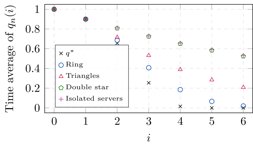
(a) Time averages.

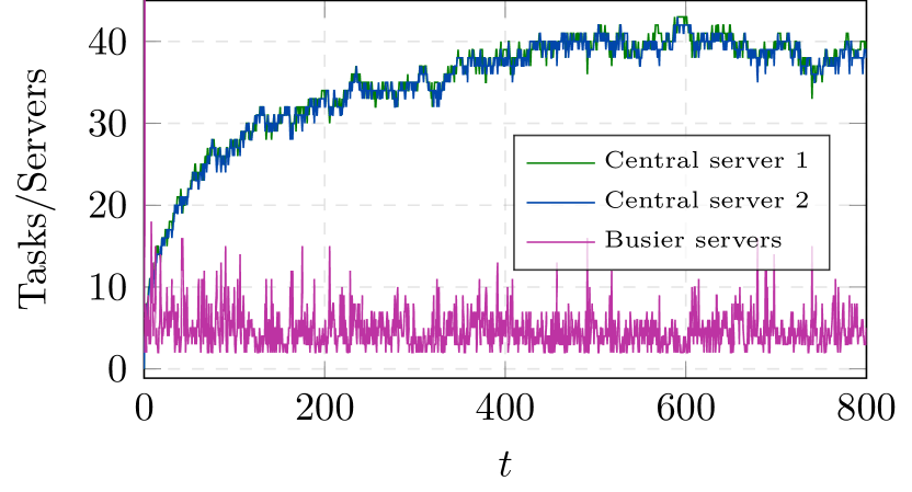
(b) Double-star topology.

Figure 3: Load balancing on static graphs with the topologies depicted in Figure 2. In all the cases the system starts empty, $n=1500$ and $\lambda_{n}=9n/10$. The plot on the left shows time averages computed over the second half of the simulation and the equilibrium point $q^{*}$ defined in Proposition 3. The plot on the right concerns the double-star topology. It shows the number of tasks at the two central servers and the number of servers that have more tasks than, or as many tasks as, the central server with the fewest tasks.

Remarkably, the performance of the double-star is equivalent to that of $n$ independent single-server queues when the graph is static. This is explained by Figure 3(b), which shows the number of tasks at the two servers placed in the center of the double-star, and the number of servers that have more tasks than, or as many tasks as, the central server with the fewest tasks. At time zero all the servers have the same number of tasks, but the percentage of servers with strictly less tasks than both of the central servers is approximately 99% or larger throughout the rest of the simulation. When a task arrives to any of these servers, the server places the task in its own queue, as if it was isolated, because its only two neighbors are the central servers, which have longer queues.

The behavior of the double-star topology may be explained as follows. The arrival rate of tasks to the central server with the fewest tasks is at least $\lambda_{n}$ times the fraction of servers that have strictly more tasks, whereas tasks leave from this server at unit rate. As a result, the number of tasks at the central servers increases quickly and remains large throughout the simulation, while the fraction of servers with strictly more tasks than the central server with the fewest tasks remains small.

A.2 Accuracy of the fluid approximation

Figures 4(a) and 4(b) show sample paths of $\boldsymbol{q}_{n}$ that remain close to the solution of (4) for the ring topology and the disjoint triangles, both in the transient and stationary regimes and for a resampling rate as low as $\mu_{n}=\log\log n$. Figures 4(c) and 4(d) show sample paths of $\boldsymbol{q}_{n}$ when the graph topology remains double-star and the resampling rate is $\mu_{n}=\log n$.

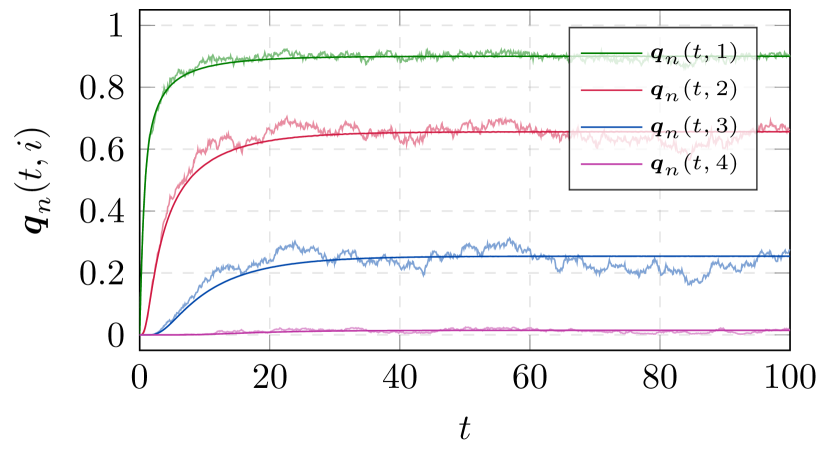
(a) Ring with $n=1500$ and $\mu_{n}=\log\log n$.

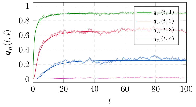
(b) Triangles with $n=1500$ and $\mu_{n}=\log\log n$.

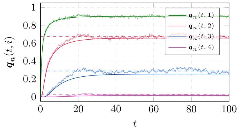
(c) Double-star with $n=1500$ and $\mu_{n}=\log n$.

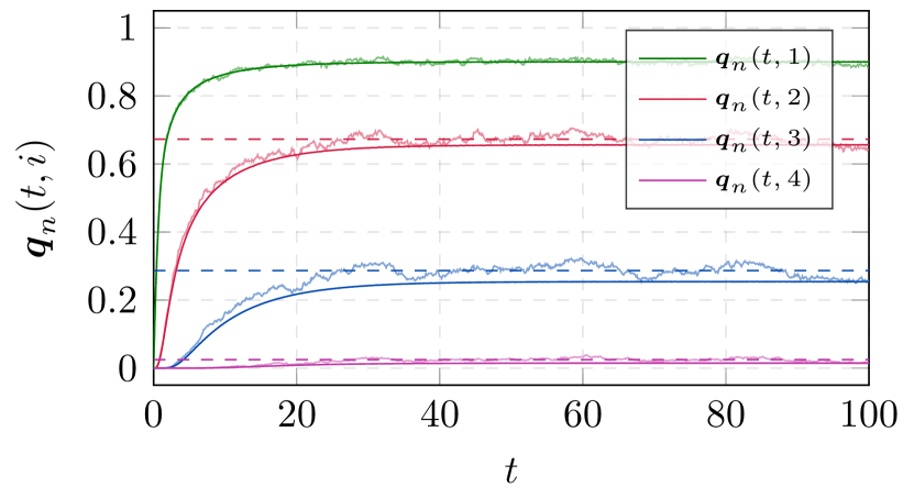
(d) Double-star with $n=5000$ and $\mu_{n}=\log n$.

Figure 4: Solution of (4) and sample paths of $\boldsymbol{q}_{n}$ for dynamic graphs. In all the cases the system starts empty, $\lambda_{n}=9n/10$ and the resampling process is Poisson. The dashed lines depicted in the two plots on the bottom correspond to time averages computed over the interval $[40,100]$.

Note that $d_{n}^{-}+1=n$ for the double-star, thus (3) does not hold when $\mu_{n}=\log n$, and in fact the approximation provided by (4) does not seem accurate. Moreover, as the number of servers increases from $n=1500$ to $n=5000$, the accuracy of the approximation does not seem to improve since the sample path of $\boldsymbol{q}_{n}$ does not get closer to the solution of (4). This indicates that Theorem 1 may not apply when $\mu_{n}=\log n$ and the graph always has a double-star topology, which suggests that some condition, besides (2), on the random graph law used to sample the graph, is necessary for the fluid limit. While the pseudo-separation property and (3) are clearly not necessary conditions for the fluid limit to hold, the latter observations indicate that the dependence of the pseudo-separation property on the maximum indegrees $d_{n}^{-}$ is not just an artifact of our proof technique but possibly a manifestation of some fundamental condition required for the fluid limit to hold.

Appendix B Proofs of various results

Proof of Lemma 1..

It follows from the mean value theorem that for each $x\in(0,1)$ and $d\geq 0$ there exists $\theta(x,d)\in(x,1)$ such that

$$\frac{1-x^{d}}{1-x}=d\left[\theta(x,d)\right]^{d-1}.$$

We conclude that

$$\left|\frac{1-x^{d}}{1-x}-d\right|=d\left|\left[\theta(x,d)\right]^{d-1}-1\right|\leq d\quad\text{for all}\quad x\in(0,1)\quad\text{and}\quad d\geq 0.$$

Given $\varepsilon>0$, there exists $k\geq 0$ such that

$$\sum_{d=k+1}^{\infty}dp(d)\leq\varepsilon.$$

Therefore, we have

$$\lim_{x\to 1^{-}}\left|\frac{\varphi(1)-\varphi(x)}{1-x}-\sum_{d=0}^{\infty}dp(d)\right| \leq\lim_{x\to 1^{-}}\sum_{d=0}^{\infty}\left|\frac{1-x^{d}}{1-x}-d\right|p(d)$$

$$\leq\lim_{x\to 1^{-}}\sum_{d=0}^{k}\left|\frac{1-x^{d}}{1-x}-d\right|p(d)+\sum_{d=k+1}^{\infty}dp(d)\leq\varepsilon.$$

Since $\varepsilon$ is arbitrary, this proves the first identity in the claim of the lemma. The second identity follows from Abel’s theorem. ∎

Proof of Proposition 2..

For the existence part, it suffices to construct occupancy processes $\boldsymbol{q}_{n}$ such that $\boldsymbol{q}_{n}(0)\Rightarrow q$ in $\ell_{1}$. The initial states $\boldsymbol{q}_{n}(0)$ can be obtained by letting $\boldsymbol{q}_{n}(0,i)$ be deterministic, equal to the number in $\left\{m/n:m=0,\dots,n\right\}$ that is closest to $q(i)$. Processes $\boldsymbol{q}_{n}$ with these initial states can be constructed as in Section 6.1. It follows from Theorem 1 that a fluid trajectory $\boldsymbol{q}$ with initial condition $q$ and continuous from $[0,\infty)$ into $\ell_{1}$ exists.

Suppose that $\boldsymbol{x}$ and $\boldsymbol{y}$ solve (6). By Lemma 1, the derivative $\varphi^{\prime}$ is continuous in $[0,1]$, thus bounded. As a result, the function $x\mapsto x\varphi(x)$ is Lipschitz in $[0,1]$. It follows from (6) that there exists a constant $L\geq 0$ such that

$$|\boldsymbol{x}(t,i)-\boldsymbol{y}(t,i)|\leq|\boldsymbol{x}(0,i)-\boldsymbol{y}(0,i)|+L\int_{0}^{t}\sum_{j=i-1}^{i+1}|\boldsymbol{x}(s,j)-\boldsymbol{y}(s,j)|ds$$

for all $i\geq 1$ and $t\geq 0$. We conclude that

$$\left|\left|\boldsymbol{x}(t)-\boldsymbol{y}(t)\right|\right|_{1}\leq\left|\left|\boldsymbol{x}(0)-\boldsymbol{y}(0)\right|\right|_{1}+3L\int_{0}^{t}\left|\left|\boldsymbol{x}(s)-\boldsymbol{y}(s)\right|\right|_{1}ds\quad\text{for all}\quad t\geq 0.$$

By Gronwall’s inequality, $\left|\left|\boldsymbol{x}(t)-\boldsymbol{y}(t)\right|\right|_{1}\leq\left|\left|\boldsymbol{x}(0)-\boldsymbol{y}(0)\right|\right|_{1}\mathrm{e}^{3Lt}$ for all $t\geq 0$. This implies that solutions are continuous with respect to the initial condition. Moreover, by setting $\boldsymbol{x}(0)=\boldsymbol{y}(0)$ we conclude that there exists a unique solution for each initial condition. ∎

Proof of Lemma 2..

Given $x,y\in\ell_{1}$, we say that $x<y$ if $x(i)<y(i)$ for all $i\geq 1$. We will prove that the following strict monotonicity property holds:

$$\boldsymbol{x}(0)<\boldsymbol{y}(0)\quad\text{implies that}\quad\boldsymbol{x}(t)<\boldsymbol{y}(t)\quad\text{for all}\quad t\geq 0.$$ (37)

First let us show that (37) implies that the lemma holds. Suppose that (37) holds and there exist fluid trajectories $\boldsymbol{x}$ and $\boldsymbol{y}$ such that $\boldsymbol{x}(0)\leq\boldsymbol{y}(0)$ but $\boldsymbol{x}(t,i)>\boldsymbol{y}(t,i)$ for some $i\geq 1$ and $t>0$. Because fluid trajectories are continuous with respect to the initial condition, there must exist fluid trajectories $\tilde{\boldsymbol{x}}$ and $\tilde{\boldsymbol{y}}$ such that

$$\tilde{\boldsymbol{x}}(0)\leq\boldsymbol{x}(0),\quad\boldsymbol{y}(0)\leq\tilde{\boldsymbol{y}}(0),\quad\tilde{\boldsymbol{x}}(0)<\tilde{\boldsymbol{y}}(0)\quad\text{and}\quad\tilde{\boldsymbol{x}}(t,i)>\tilde{\boldsymbol{y}}(t,i).$$

But this would lead to a contradiction since the last two inequalities violate (37). Hence, proving (37) is equivalent to proving the lemma.

We establish (37) by contradiction. For this purpose, suppose that there exist two fluid trajectories $\boldsymbol{x}$ and $\boldsymbol{y}$ such that $\boldsymbol{x}(0)<\boldsymbol{y}(0)$ but (37) does not hold, and thus

$$\tau\vcentcolon=\inf\left\{t\geq 0:\boldsymbol{x}(t,i)\geq\boldsymbol{y}(t,i)\ \text{for some}\ i\geq 1\right\}<\infty.$$

Observe that for each $i\geq 1$ we have

$$\dot{\boldsymbol{x}}(i)-\dot{\boldsymbol{y}}(i) =\lambda\left[\boldsymbol{x}(i-1)\varphi\left(\boldsymbol{x}(i-1)\right)-\boldsymbol{y}(i-1)\varphi\left(\boldsymbol{y}(i-1)\right)\right]$$

$$-\lambda\left[\boldsymbol{x}(i)\varphi\left(\boldsymbol{x}(i)\right)-\boldsymbol{y}(i)\varphi\left(\boldsymbol{y}(i)\right)\right]-\left[\boldsymbol{x}(i)-\boldsymbol{y}(i)\right]+\boldsymbol{x}(i+1)-\boldsymbol{y}(i+1)$$

$$\leq\lambda\left[\boldsymbol{y}(i)\varphi\left(\boldsymbol{y}(i)\right)-\boldsymbol{x}(i)\varphi\left(\boldsymbol{x}(i)\right)\right]+\left[\boldsymbol{y}(i)-\boldsymbol{x}(i)\right]$$

almost everywhere in $[0,\tau]$. For the inequality note that $x\mapsto x\varphi(x)$ is increasing.

By Lemma 1, $\varphi^{\prime}$ is bounded in $[0,1]$, so there exists $L\geq 0$ such that

$$\boldsymbol{y}(i)\varphi\left(\boldsymbol{y}(i)\right)-\boldsymbol{x}(i)\varphi\left(\boldsymbol{x}(i)\right) =\left|\boldsymbol{y}(i)\varphi\left(\boldsymbol{y}(i)\right)-\boldsymbol{x}(i)\varphi\left(\boldsymbol{x}(i)\right)\right|$$

$$\leq L\left|\boldsymbol{y}(i)-\boldsymbol{x}(i)\right|=L\left[\boldsymbol{y}(i)-\boldsymbol{x}(i)\right]$$

in the interval $[0,\tau]$ for all $i\geq 1$. Therefore,

$$\dot{\boldsymbol{x}}(i)-\dot{\boldsymbol{y}}(i)\leq(\lambda L+1)\left[\boldsymbol{y}(i)-\boldsymbol{x}(i)\right]=-(\lambda L+1)\left[\boldsymbol{x}(i)-\boldsymbol{y}(i)\right]$$

almost everywhere in the interval $[0,\tau]$. It follows that

$$\boldsymbol{x}(t,i)-\boldsymbol{y}(t,i)\leq\left[\boldsymbol{x}(0,i)-\boldsymbol{y}(0,i)\right]\mathrm{e}^{-(\lambda L+1)t}<0\quad\text{for all}\quad i\geq 1\quad\text{and}\quad t\in[0,\tau].$$

But this contradicts the definition of $\tau$, thus (37) must hold. ∎

Proof of Proposition 4..

By Lemma 2, it suffices to prove the proposition in the following two cases: $\boldsymbol{q}(0)\geq q^{*}$ and $\boldsymbol{q}(0)\leq q^{*}$. We only prove the proposition in the case $\boldsymbol{q}(0)\geq q^{*}$ because the proof is analogous in the other case.

Suppose then that $\boldsymbol{q}(0)\geq q^{*}$. We proceed as in [15, Propostion 4.5], letting

$$\boldsymbol{s}(t,i)\vcentcolon=\sum_{j=i}^{\infty}\boldsymbol{q}(t,j)\quad\text{for all}\quad i\geq 1\quad\text{and}\quad t\geq 0,$$

$$\dot{\boldsymbol{s}}(t,i)\vcentcolon=\sum_{j=i}^{\infty}\dot{\boldsymbol{q}}(t,j)=\lambda\boldsymbol{q}(t,i-1)\varphi\left(\boldsymbol{q}(t,i-1)\right)-\boldsymbol{q}(t,i)\quad\text{for all}\quad i\geq 1\quad\text{and}\quad t\geq 0.$$

Since fluid trajectories take values in $Q\subset\ell_{1}$, both sums converge pointwise; i.e., for each fixed $t\geq 0$. It follows from (6) that $|\dot{\boldsymbol{q}}(i)|$ is bounded by $\lambda+1$ for all $i\geq 1$, thus $\boldsymbol{q}(i)$ is Lipschitz of modulus $\lambda+1$. Moreover, because $\varphi^{\prime}$ is bounded in the interval $[0,1]$, there exists $M\geq 0$ such that the function $x\mapsto x\varphi(x)$ is Lipschitz of modulus $M$. Therefore,

$$\sum_{j=i}^{k}\dot{\boldsymbol{q}}(j)=\lambda\left[\boldsymbol{q}(i-1)\varphi\left(\boldsymbol{q}(i-1)\right)-\boldsymbol{q}(k)\varphi(\boldsymbol{q}(k))\right]-\left[\boldsymbol{q}(i)-\boldsymbol{q}(k+1)\right]$$

is Lipschitz of modulus $4\max\{\lambda(\lambda+1)M,\lambda+1\}$ for all $k\geq i$. By the Arezlá-Ascoli theorem, the above partial sums converge uniformly over compact sets to $\dot{\boldsymbol{s}}(i)$. Hence, it follows from [27, Theorem 7.17] that $\boldsymbol{s}(i)$ also converges uniformly over compact sets and $\dot{\boldsymbol{s}}(t,i)$ is the derivative of $\boldsymbol{s}(i)$ at $t$ for all $t>0$.

Since $\varphi^{\prime}$ is bounded in $[0,1]$, there exists a constant $L\geq 0$ such that $\varphi$ is a Lipschitz function of modulus $L$. From this observation we conclude that

$$\dot{\boldsymbol{s}}(i) =\lambda\boldsymbol{q}(i-1)\varphi\left(\boldsymbol{q}(i-1)\right)-\boldsymbol{q}(i)$$

$$=\lambda\left[\boldsymbol{q}(i-1)\varphi\left(\boldsymbol{q}(i-1)\right)-q^{*}(i-1)\varphi\left(q^{*}(i-1)\right)\right]+q^{*}(i)-\boldsymbol{q}(i)$$

$$=\lambda\left[\boldsymbol{q}(i-1)-q^{*}(i-1)\right]\varphi\left(\boldsymbol{q}(i-1)\right)+\lambda q^{*}(i-1)\left[\varphi\left(\boldsymbol{q}(i-1)\right)-\varphi\left(q^{*}(i-1)\right)\right]$$

$$+q^{*}(i)-\boldsymbol{q}(i)$$

$$\leq\lambda(1+L)\left[\boldsymbol{q}(i-1)-q^{*}(i-1)\right]-\left[\boldsymbol{q}(i)-q^{*}(i)\right]\quad\text{for all}\quad i\geq 1.$$

For the inequality observe that $\boldsymbol{q}(t,i-1)\geq q^{*}(i-1)$ by assumption and Lemma 2. In addition, note that $\varphi$ is an increasing function, thus $\varphi\left(\boldsymbol{q}(t,i-1)\right)\geq\varphi\left(q^{*}(i-1)\right)$ for all $i\geq 1$ and $t\geq 0$. Integrating on both sides of the inequality, we conclude that

$$\int_{0}^{t}\left[\boldsymbol{q}(s,i)-q^{*}(i)\right]ds\leq\boldsymbol{s}(0,i)-\boldsymbol{s}(t,i)+\lambda(1+L)\int_{0}^{t}\left[\boldsymbol{q}(s,i-1)-q^{*}(i-1)\right]ds.$$

Setting $i=1$, we obtain

$$\int_{0}^{t}\left[\boldsymbol{q}(s,1)-q^{*}(1)\right]ds\leq\boldsymbol{s}(0,1)-\boldsymbol{s}(t,1)\leq\boldsymbol{s}(0,1),$$

and taking the limit as $t\to\infty$, we get

$$\int_{0}^{\infty}\left[\boldsymbol{q}(s,1)-q^{*}(1)\right]ds\leq\boldsymbol{s}(0,1)<\infty.$$

By induction in $i$, we conclude that

$$\int_{0}^{\infty}\left[\boldsymbol{q}(s,i)-q^{*}(i)\right]ds\leq\boldsymbol{s}(0,i)+\lambda(1+L)\int_{0}^{\infty}\left[\boldsymbol{q}(s,i-1)-q^{*}(i-1)\right]ds<\infty\quad\text{if}\quad i\geq 1.$$

Recall that $\boldsymbol{q}(t,i)\geq q^{*}(t,i)$ for all $t\geq 0$, thus $\boldsymbol{q}(t,i)\to q^{*}(i)$ as $t\to\infty$ for all $i\geq 1$. ∎

Proof of Corollary 2..

In order to compute the limit of $R_{n}$, note that

$$\left|\left|\left|q_{n}\right|\right|_{1}-\left|\left|q^{*}\right|\right|_{1}\right|\leq\left|\left|q_{n}-q_{*}\right|\right|_{1}\quad\text{for all}\quad n\geq 1.$$

The limit $q_{n}\Rightarrow q^{*}$ in $\ell_{1}$ is equivalent to $\left|\left|q_{n}-q^{*}\right|\right|_{1}\Rightarrow 0$, and hence $\left|\left|q_{n}\right|\right|_{1}\Rightarrow\left|\left|q_{*}\right|\right|_{1}$. By Lemma 3, the sequence $\left\{\left|\left|q_{n}\right|\right|_{1}:n\geq 1\right\}$ is uniformly integrable, so the latter limit also holds in expectation. We conclude that

$$\lim_{n\to\infty}R_{n}=\lim_{n\to\infty}\frac{n}{\lambda_{n}}E\left[\left|\left|q_{n}\right|\right|_{1}-1\right]=\frac{\left|\left|q^{*}\right|\right|_{1}-1}{\lambda}.$$

This completes the proof. ∎

Proof of Lemma 5.

The process that describes the times of departures from the servers can be described as follows. Every server experiences potential departures as a Poisson process of unit intensity and if a server has at least one task at the time of a potential departure, then a task departs from the server. Given $\sigma_{n}^{m}-\sigma_{n}^{m-1}$, the number of arrivals and potential departures in $\left(\sigma_{n}^{m-1},\sigma_{n}^{m}\right]$ are Poisson distributed with mean $\lambda_{n}\left(\sigma_{n}^{m}-\sigma_{n}^{m-1}\right)$ and $n\left(\sigma_{n}^{m}-\sigma_{n}^{m-1}\right)$, respectively. Thus, the first claim of the lemma holds.

Assume that condition (c) of Proposition 1 holds. In order to establish (21), define

$$\Gamma_{n}(t)\vcentcolon=\sum_{m=1}^{\mathcal{R}_{n}(t)+1}\left(\sigma_{n}^{m}-\sigma_{n}^{m-1}\right)^{2}\quad\text{and}\quad\varphi_{n}(t)\vcentcolon=E\left[\Gamma_{n}(t)\right]\quad\text{for all}\quad t\geq 0.$$

Applying a renewal argument we conclude that

$$E\left[\Gamma_{n}(t)\nonscript\;\middle|\nonscript\;\sigma_{n}^{1}=\sigma\right]=\sigma^{2}+\varphi_{n}(t-\sigma)\mathbbm{1}_{\left\{\sigma\leq t\right\}}\quad\text{for all}\quad t,\sigma\geq 0.$$

Hence, if we let $F_{n}(\sigma)\vcentcolon=P\left(\sigma_{n}^{1}\leq\sigma\right)$ denote the cumulative distribution function of the holding times, then integration with respect to $F_{n}$ yields

$$\varphi_{n}(t)=\int_{0}^{\infty}E\left[\Gamma_{n}(t)\nonscript\;\middle|\nonscript\;\sigma_{n}^{1}=\sigma\right]dF_{n}(\sigma)=E\left[\left(\sigma_{n}^{1}\right)^{2}\right]+\int_{0}^{t}\varphi_{n}(t-\sigma)dF_{n}(\sigma)\quad\text{for all}\quad t\geq 0.$$

By [20, Theorem 12.24], the solution of this renewal equation is

$$\varphi_{n}(t)=E\left[\left(\sigma_{n}^{1}\right)^{2}\right]+\int_{0}^{t}E\left[\left(\sigma_{n}^{1}\right)^{2}\right]dR_{n}(t)=E\left[\left(\sigma_{n}^{1}\right)^{2}\right]\left[1+R_{n}(t)\right]\quad\text{for all}\quad t\geq 0,$$

where $R_{n}(t)=E\left[\mathcal{R}_{n}(t)\right]$. Also, condition (c) of Proposition 1 implies that $\sigma_{n}^{1}=\sigma_{1}^{1}/\mu_{n}$, and the elementary renewal theorem yields $R_{n}(t)/\mu_{n}\to t$ as $n\to\infty$. Therefore,

$$\lim_{n\to\infty}\mu_{n}\varphi_{n}(t)=\lim_{n\to\infty}E\left[\left(\sigma_{1}^{1}\right)^{2}\right]\frac{1+R_{n}(t)}{\mu_{n}}=E\left[\left(\sigma_{1}^{1}\right)^{2}\right]t.$$

This completes the proof. ∎

Proof of Lemma 6.

The topology of $D_{\mathbbm{R}^{\mathbbm{N}}}[0,\infty)$ is compatible with the metric

$$\eta(\boldsymbol{x},\boldsymbol{y})\vcentcolon=\sum_{T=1}^{\infty}\frac{\min\left\{\sup_{t\in[0,T]}d\left(\boldsymbol{x}(t),\boldsymbol{y}(t)\right),1\right\}}{2^{T}}\quad\text{for all}\quad\boldsymbol{x},\boldsymbol{y}\in D_{\mathbbm{R}^{\mathbbm{N}}}[0,\infty).$$

It is straightforward to check that (a) implies (b), thus we only prove that (b) implies (a). For this purpose, fix $\varepsilon>0$ and assume that

$$\boldsymbol{x}_{n}(i)\Rightarrow 0\quad\text{in}\quad D_{\mathbbm{R}}[0,T]\quad\text{as}\quad n\to\infty\quad\text{for all}\quad i\geq 0\quad\text{and}\quad T\geq 0.$$

Choose $l$ and $m$ such that

$$\sum_{T=l+1}^{\infty}\frac{1}{2^{T}}\leq\frac{\varepsilon}{2}\quad\text{and}\quad\sum_{i=m}^{\infty}\frac{1}{2^{i}}\leq\frac{\varepsilon}{4l}.$$

By the choice of $l$, we have

$$P\left(\eta(\boldsymbol{x}_{n},0)\geq\varepsilon\right)\leq\sum_{T=1}^{l}P\left(\sup_{t\in[0,T]}d\left(\boldsymbol{x}_{n}(t),0\right)\geq\frac{\varepsilon}{2l}\right),$$

and by the choice of $m$,

$$P\left(\sup_{t\in[0,T]}d\left(\boldsymbol{x}_{n}(t),0\right)\geq\frac{\varepsilon}{2l}\right)\leq\sum_{i=0}^{m-1}P\left(\left|\left|\boldsymbol{x}_{n}(i)\right|\right|_{T}\geq\frac{\varepsilon}{4lm}\right).$$

Therefore, we have

$$P\left(\eta(\boldsymbol{x}_{n},0)\geq\varepsilon\right)\leq\sum_{T=1}^{l}\sum_{i=0}^{m-1}P\left(\left|\left|\boldsymbol{x}_{n}(i)\right|\right|_{T}\geq\frac{\varepsilon}{4lm}\right),$$

and the right-hand side converges to zero as $n\to\infty$ by assumption; indeed, note that weak convergence to zero is equivalent to convergence in probability to zero. ∎

Proof of Lemma 9.

Let $\rho_{j}$ be the metric of $S_{j}$ and endow $\Pi$ with the metric defined by

$$\varrho\left(\left(y_{1},\dots,y_{m}\right),\left(z_{1},\dots,z_{m}\right)\right)\vcentcolon=\max_{j=1,\dots,m}\rho_{j}\left(y_{j},z_{j}\right)\quad\text{for all}\quad\left(y_{1},\dots,y_{m}\right),\left(z_{1},\dots,z_{m}\right)\in\Pi,$$

which is compatible with the product topology. If $f:\Pi\longrightarrow\mathbbm{R}$ is continuous and bounded, then $y_{1}\mapsto f(y_{1},x_{2},\dots,x_{m})$ defines a continuous and bounded function on $S_{1}$. Hence,

$$\lim_{k\to\infty}E\left[f\left(X_{k}^{1},x_{2},\dots,x_{m}\right)\right]=E\left[f\left(X_{1},x_{2},\dots,x_{m}\right)\right],$$

and we conclude that $\left(X_{k}^{1},x_{2},\dots,x_{m}\right)\Rightarrow\left(X_{1},x_{2},\dots,x_{m}\right)$ in $\Pi$ as $k\to\infty$. Moreover,

$$P\left(\varrho\left(\left(X_{k}^{1},X_{k}^{2},\dots,X_{k}^{m}\right),\left(X_{k}^{1},x_{2},\dots,x_{m}\right)\right)\geq\varepsilon\right)\leq\sum_{j=2}^{m}P\left(\rho_{j}\left(X_{k}^{j},x_{j}\right)\geq\varepsilon\right),$$

and for every $\varepsilon>0$ the right-hand side goes to zero as $k\to\infty$ by assumption. It follows from [4, Theorem 3.1] that $\left(X_{k}^{1},X_{k}^{2},\dots,X_{k}^{m}\right)\Rightarrow\left(X_{1},x_{2},\dots,x_{m}\right)$ in $\Pi$. ∎

Addition to Remark 13.

Let $S_{\mathbbm{R}}[0,\infty)$ denote the space of real càdlàg functions endowed with the Skorohod $J_{1}$-topology, and let $\Pi\vcentcolon=S_{\mathbbm{R}}[0,\infty)\times S_{\mathbbm{R}}[0,\infty)\times S_{\ell_{1}}[0,\infty)\times S_{\mathbbm{R}^{\mathbbm{N}}}[0,\infty)$ with the product topology and the Borel $\sigma$-algebra. The right-hand side of (29) defines a measurable function from $\Pi$ into $\mathbbm{R}$, thus the probability that (29) holds is equal to

$$P\left(\left(\mathcal{N}_{k}^{a},\mathcal{R}_{k},\boldsymbol{q}_{k},\boldsymbol{v}_{k}\right)\in A\right)$$

for some set $A$ in the Borel $\sigma$-algebra of $\Pi$. Skorohod’s representation theorem implies that the law of $\left(\mathcal{N}_{k}^{a},\mathcal{R}_{k},\boldsymbol{q}_{k},\boldsymbol{v}_{k}\right)$ is as in Section 6.2, so the latter probability equals one.

As an example, let us establish that $\boldsymbol{u}_{k}(t,i)$ is a measurable function of $\left(\mathcal{N}_{k}^{a},\mathcal{R}_{k},\boldsymbol{q}_{k},\boldsymbol{v}_{k}\right)$ when (16) holds. For this purpose, consider partitions $0=t_{0}^{l}<\dots<t_{J_{l}}^{l}=t$ such that

$$\lim_{l\to\infty}\max_{0\leq j\leq J_{l}-1}\left(t_{j+1}^{l}-t_{j}^{l}\right)=0.$$

In addition, define $s_{m}^{l}\vcentcolon=t_{j_{m}^{l}}^{l}$ for each $l,m\geq 1$, where

$$j_{m}^{l}\vcentcolon=\max\left\{0\leq j\leq J_{l}:\mathcal{N}_{k}^{a}\left(t_{j}^{l}\right)<m\ \text{and}\ j=0\ \text{or}\ \mathcal{R}_{k}\left(t_{j}^{l}\right)>\mathcal{R}_{k}\left(t_{j-1}^{l}\right)\right\}.$$

Because the finite-dimensional projections $\pi_{t_{1},\dots,t_{l}}:\Pi\longrightarrow\mathbbm{R}^{l}$ are measurable for all $t_{1},\dots,t_{l}\geq 0$, we conclude that $j_{m}^{l}$ is measurable as a function from $\Pi$ into $\mathbbm{R}$. Also,

$$\lim_{l\to\infty}s_{m}^{l}=\max\left\{\sigma_{k}^{j}:\sigma_{k}^{j}<\tau_{k}^{m}\right\},$$

and $s_{m}^{l}\geq\max\left\{\sigma_{k}^{j}:\sigma_{k}^{j}<\tau_{k}^{m}\right\}$ for all large enough $l$. Since $\boldsymbol{q}_{k}$ is right-continuous,

$$\lim_{l\to\infty}\boldsymbol{q}_{k}\left(s_{m}^{l},i\right)=\bar{q}_{k}^{m}(i).$$

It follows that

$$\boldsymbol{u}_{k}(t,i)=\lim_{l\to\infty}\frac{1}{k}\sum_{m=1}^{l}\sum_{j=1}^{J_{l}}\beta_{k}\left(\boldsymbol{q}_{k}\left(t_{j}^{l},i\right)\right)\mathbbm{1}_{\left\{j=j_{m}^{l}\right\}}\mathbbm{1}_{\left\{m\leq\mathcal{N}_{k}^{a}(t)\right\}}.$$

Each of the functions inside of the limit sign is measurable from $\Pi$ into $\mathbbm{R}$ and the limit of measurable functions is a measurable function as well. Hence, we conclude that $\boldsymbol{u}_{k}(t,i)$ is a measurable function of $\left(\mathcal{N}_{k}^{a},\mathcal{R}_{k},\boldsymbol{q}_{k},\boldsymbol{v}_{k}\right)$. ∎

Proof of Lemma 11.

In order to prove (32), fix an arbitrary $\varepsilon>0$ and note that

$$\sup_{x\in[0,d/n)}\left|\alpha_{n}(d+1,x)-x^{d+1}\right|=\sup_{x\in[0,d/n)}x^{d+1}\leq\varepsilon$$

for all sufficiently large $n$. Now consider the function $f:[0,1]^{d+1}\longrightarrow\mathbbm{R}$ that assigns to each vector the product of its entries. The bound

$$\max_{0\leq k\leq d}\left|\frac{nx-k}{n-k}-x\right|=\max_{0\leq k\leq d}\left|\frac{k(x-1)}{n-k}\right|\leq\frac{d}{n-d}\quad\text{for all}\quad x\in\left[0,1\right],$$

and the uniform continuity of $f$ imply that

$$\sup_{x\in[d/n,1]}\left|\alpha_{n}(d+1,x)-x^{d+1}\right|\leq\sup_{x\in[0,1]}\left|f\left(x,\frac{nx-1}{n-1},\dots,\frac{nx-d}{n-d}\right)-f(x,x,\dots,x)\right|\leq\varepsilon$$

for all large enough $n$. Because $\varepsilon$ is arbitrary, this proves (32).

For (33), observe that

$$\beta_{n}(x)-x\varphi(x)=\sum_{d=0}^{\infty}\left[\alpha_{n}(d+1,x)p_{n}(d)-x^{d+1}p(d)\right]\quad\text{for all}\quad x\in[0,1]\quad\text{and}\quad n\geq 1.$$

Fix $\theta\in[0,1)$ and some $k\geq 0$. If $x\in[0,\theta]$, then

$$\left|\beta_{n}(x)-x\varphi(x)\right| \leq\sum_{d=0}^{k}\left|\alpha_{n}(d+1,x)p_{n}(d)-x^{d+1}p(d)\right|+\sum_{d=k+1}^{\infty}\alpha_{n}(d+1,x)+\sum_{d=k+1}^{\infty}x^{d+1}$$

$$\leq\sum_{d=0}^{k}\left|\alpha_{n}(d+1,x)-x^{d+1}\right|p_{n}(d)+\sum_{d=0}^{k}x^{d+1}\left|p_{n}(d)-p(d)\right|+2\sum_{d=k+1}^{\infty}x^{d+1}$$

$$\leq\sum_{d=0}^{k}\left|\alpha_{n}(d+1,x)-x^{d+1}\right|+\sum_{d=0}^{k}\left|p_{n}(d)-p(d)\right|+\frac{2\theta^{k+2}}{1-\theta}.$$

For the second inequality, note that $\alpha_{n}(d+1,x)\leq x^{d+1}$ for all $d\geq 0$ and $n\geq 1$. Given an arbitrary $\varepsilon>0$, we may choose $k$ such that $2\theta^{k+2}\leq(1-\theta)\varepsilon$. Then

$$\lim_{n\to\infty}\sup_{x\in[0,\theta]}\left|\beta_{n}(x)-x\varphi(x)\right|\leq\lim_{n\to\infty}\left[\sum_{d=0}^{k}\sup_{x\in[0,1]}\left|\alpha_{n}(d+1,x)-x^{d+1}\right|+\sum_{d=0}^{k}\left|p_{n}(d)-p(d)\right|\right]+\varepsilon.$$

Since $\varepsilon$ is arbitrary, we conclude from (2) and (32) that (33) holds.

Suppose now that $p(\infty)=0$ and thus $\varphi(1)=1$. It follows from Abel’s theorem that $\varphi$ is continuous on $[0,1]$. Hence, if $\varepsilon>0$, then there exists $\delta\in(0,1)$ such that

$$|x\varphi(x)-y\varphi(y)|\leq\frac{\varepsilon}{3}\quad\text{for all}\quad x,y\in[0,1]\quad\text{such that}\quad|x-y|\leq\delta.$$

Choose $\theta\in(1-\delta,1)$ and note that (33) implies that there exists $m$ such that

$$|\beta_{n}(x)-x\varphi(x)|\leq\frac{\varepsilon}{6}\quad\text{for all}\quad x\in[0,\theta]\quad\text{and}\quad n\geq m.$$

If $x\in(\theta,1]$, then we have

$$|\beta_{n}(x)-x\varphi(x)| \leq|\beta_{n}(x)-\beta_{n}(\theta)|+|\beta_{n}(\theta)-\theta\varphi(\theta)|+|\theta\varphi(\theta)-x\varphi(x)|$$

$$\leq 1-\beta_{n}(\theta)+|\beta_{n}(\theta)-\theta\varphi(\theta)|+|\theta\varphi(\theta)-x\varphi(x)|$$

$$\leq 1-\theta\varphi(\theta)+2|\beta_{n}(\theta)-\theta\varphi(\theta)|+|\theta\varphi(\theta)-x\varphi(x)|\leq\varepsilon\quad\text{for all}\quad n\geq m.$$

For the second inequality, note that $\beta_{n}$ is nondecreasing and $\beta_{n}(1)=1$ because $\alpha_{n}(d+1)$ has these properties for each $d\leq n-1$. For the last inequality, recall that $\varphi(1)=1$ by assumption, and note that $|1-x|<|1-\theta|<\delta$. Since $\varepsilon$ is arbitrary, (34) holds. ∎

Appendix C Construction of sample paths

The processes $\boldsymbol{q}_{n}$ and $\boldsymbol{X}_{n}$ are constructed inductively. At time zero,

$$\boldsymbol{X}_{n}(0)=X_{n}\quad\text{and}\quad\boldsymbol{q}_{n}(0,i)=q_{n}(i)=\frac{1}{n}\sum_{u=1}^{n}\mathbbm{1}_{\left\{X_{n}(u)\geq i\right\}}\quad\text{for all}\quad i\geq 0.$$

We refer to time zero and the times of arrivals and departures of tasks as event times. If both processes have already been defined up to event time $\tau$, then they remain constant until the next event occurs.

Let $\boldsymbol{q}_{n}^{\tau}$ denote the stopped process defined as

$$\boldsymbol{q}_{n}^{\tau}(t)\vcentcolon=\boldsymbol{q}_{n}(t)\quad\text{if}\quad 0\leq t\leq\tau\quad\text{and}\quad\boldsymbol{q}_{n}^{\tau}(t)\vcentcolon=\boldsymbol{q}_{n}(\tau)\quad\text{if}\quad t>\tau.$$

The next event after $\tau$ corresponds to the first jump after $\tau$ of one the processes

$$t\mapsto\mathcal{N}_{n}^{a}(t)\quad\text{and}\quad t\mapsto\mathcal{N}_{i}^{d}\left(n\int_{0}^{t}\left[\boldsymbol{q}_{n}^{\tau}(s,i)-\boldsymbol{q}_{n}^{\tau}(s,i+1)\right]ds\right).$$ (38)

Only finitely many of these processes have a positive intensity since the initial number of tasks in the system is finite by assumption, hence the time of the next event is strictly larger than $\tau$. The intensity of process $i$ on the right corresponds to the departure rate from servers with exactly $i$ tasks, a jump of this process indicates such a departure.

Once the time of the next event is determined, the processes $\boldsymbol{q}_{n}$ and $\boldsymbol{X}_{n}$ are updated in different ways depending on the type of the new event. If the first event after $\tau$ is an arrival that occurs at time $\tau_{n}^{m}$, then we set

$$\boldsymbol{q}_{n}\left(\tau_{n}^{m},i\right)=\boldsymbol{q}_{n}\left(\tau_{n}^{m-},i\right)+\frac{1}{n}\left[I_{n}^{m}\left(\boldsymbol{X}_{n}\left(\tau_{n}^{m-}\right),i-1\right)-I_{n}^{m}\left(\boldsymbol{X}_{n}\left(\tau_{n}^{m-}\right),i\right)\right]\quad\text{for all}\quad i\geq 1.$$

The difference between the last two terms equals one if the task is placed in the queue of a server with exactly $i-1$ tasks and equals zero otherwise. In addition, we let

$$v_{n}^{m}=\min\underset{v}{\text{argmin}}\left\{\boldsymbol{X}_{n}\left(\tau_{n}^{m-},v\right):v=u_{n}^{m}\ \text{or}\ \left(u_{n}^{m},v\right)\in\boldsymbol{E}_{n}\left(\tau_{n}^{m-}\right)\right\}$$

be the server with the smallest index among the servers with the least number of tasks in the neighborhood of $u_{n}^{m}$ and we set

$$\boldsymbol{X}_{n}\left(\tau_{n}^{m},v\right)=\boldsymbol{X}_{n}\left(\tau_{n}^{m-},v\right)+\mathbbm{1}_{\left\{v=v_{n}^{m}\right\}}\quad\text{for all}\quad v\in V_{n}.$$

In order to choose the server $v_{n}^{m}$ in the neighborhood of $u_{n}^{m}$ that will receive the new task, we break ties between servers with the least number of tasks by selecting the server with the smallest index. But any other criterion could be used instead.

Suppose instead that the first event after $\tau$ is a departure from a server with exactly $i$ tasks, triggered by a jump of process $i$ on the right of (38). We denote the time of this departure by $\tau_{i,n}^{m}$ and we set

$$\boldsymbol{q}_{n}\left(\tau_{i,n}^{m},j\right)=\boldsymbol{q}_{n}\left(\tau_{i,n}^{m-},j\right)-\frac{1}{n}\mathbbm{1}_{\left\{j=i\right\}}\quad\text{for all}\quad j\geq 1.$$

In addition, we use the random variable $U_{i,n}^{m}$ to select a server $v_{i,n}^{m}$ uniformly at random among all the servers $v$ with exactly $i$ tasks: $\boldsymbol{X}_{n}\left(\tau_{i,n}^{m-},v\right)=i$. Then we set

$$\boldsymbol{X}_{n}\left(\tau_{i,n}^{m},v\right)=\boldsymbol{X}_{n}\left(\tau_{i,n}^{m-},v\right)-\mathbbm{1}_{\left\{v_{i,n}^{m}=v\right\}}\quad\text{for all}\quad v\in V_{n}.$$

The above construction determines $\boldsymbol{X}_{n}$ and $\boldsymbol{q}_{n}$ on a set of probability one that excludes certain events of probability zero, such as tasks arriving and departing simultaneously. Both $\boldsymbol{q}_{n}$ and $\boldsymbol{X}_{n}$ are piecewise constant càdlàg processes defined on $[0,\infty)$. In addition, the jumps of $\boldsymbol{q}_{n}$ are of size $1/n$ and $\boldsymbol{X}_{n}$ has jumps of unit size.

Appendix D Tightness of occupancy processes

The topology of $D_{\ell_{1}}[0,\infty)$ is compatible with the metric defined by

$$\rho(\boldsymbol{x},\boldsymbol{y})\vcentcolon=\sum_{T=1}^{\infty}\frac{\min\left\{\sup_{t\in[0,T]}\left|\left|\boldsymbol{x}(t)-\boldsymbol{y}(t)\right|\right|_{1},1\right\}}{2^{T}}\quad\text{for all}\quad\boldsymbol{x},\boldsymbol{y}\in D_{\ell_{1}}[0,\infty).$$

Hence, it follows from Prohorov’s theorem that in order to prove Proposition 10, it is enough to show that $\left\{\boldsymbol{q}_{n}:n\geq 1\right\}$ is tight in $D_{\ell_{1}}[0,\infty)$, which we proceed to do.

Consider a function $\boldsymbol{x}\in D_{\ell_{1}}[0,\infty)$. Its local moduli of continuity is defined as

$$w_{T}(\boldsymbol{x},h)\vcentcolon=\sup\left\{\left|\left|\boldsymbol{x}(s)-\boldsymbol{x}(t)\right|\right|_{1}:s,t\in[0,T]\ \text{and}\ |s-t|\leq h\right\}$$

for all $h>0$ and $T\geq 0$. The modified local moduli of continuity is defined as

$$\tilde{w}_{T}(\boldsymbol{x},h)\vcentcolon=\inf_{\mathcal{I}}\max_{I\in\mathcal{I}}\sup_{s,t\in I}\left|\left|\boldsymbol{x}(s)-\boldsymbol{x}(t)\right|\right|_{1}.$$

Here the infimum extends over all partitions $\mathcal{I}$ of $[0,T)$ into subintervals $I=[u,v)$ such that $v-u\geq h$ if $v<T$. By [20, Theorems 23.8 and 23.9], and the fact that

$$\tilde{w}_{T}(\boldsymbol{x},h)\leq w_{T}(\boldsymbol{x},h)\quad\text{for all}\quad\boldsymbol{x}\in D_{\ell_{1}}[0,\infty),\quad h>0\quad\text{and}\quad T\geq 0,$$

the tightness of $\left\{\boldsymbol{q}_{n}:n\geq 1\right\}$ can be established by proving the following properties.

1. $\left\{\boldsymbol{q}_{n}(t):n\geq 1\right\}$ is tight in $\ell_{1}$ for all $t$ in some dense subset of $[0,\infty)$.

2. If $T>0$, then

   $$\lim_{h\to 0}\limsup_{n\to\infty}E\left[\min\left\{w_{T}(\boldsymbol{q}_{n},h),1\right\}\right]=0.$$

The following two lemmas are used to establish property (a).

Lemma 12.

Let $\left\{q_{n}:n\geq 1\right\}$ be a sequence of random variables with values in

$$Q\vcentcolon=\left\{q\in\ell_{1}:0\leq q(i+1)\leq q(i)\leq q(0)=1\ \text{for all}\ i\geq 1\right\}.$$

The sequence $\left\{q_{n}:n\geq 1\right\}$ is tight in $\ell_{1}$ if and only if

$$\lim_{m\to\infty}\limsup_{n\to\infty}P\left(\sum_{i>m}q_{n}(i)>\varepsilon\right)=0\quad\text{for all}\quad\varepsilon>0.$$

The previous lemma is taken from [25, Lemma 2], where the proof can be found. We use it in the following lemma in order to establish property (a).

Lemma 13.

If $\left\{\boldsymbol{q}_{n}(0):n\geq 1\right\}$ is tight in $\ell_{1}$, then so is $\left\{\boldsymbol{q}_{n}(t):n\geq 1\right\}$ for all $t\geq 0$.

Proof.

By Lemma 12, it suffices to prove that

$$\lim_{m\to\infty}\limsup_{n\to\infty}P\left(\sum_{i>m}\boldsymbol{q}_{n}(t,i)>\varepsilon\right)=0\quad\text{for all}\quad\varepsilon,t>0.$$ (39)

Fix any $\varepsilon,t>0$, let $\theta\vcentcolon=t(\mathrm{e}-1)+1$ and choose constants $k,\delta_{0},\delta_{1}>0$ such that

$$\delta_{0}+\delta_{1}\lambda\theta<\varepsilon\quad\text{and}\quad\delta_{1}>\delta_{0}+\frac{\lambda\theta}{k}.$$

In addition, fix $n_{0}\geq 0$ such that all $n\geq n_{0}$ satisfy:

$$\delta_{0}+\frac{\delta_{1}\lambda_{n}\theta}{n}<\varepsilon,$$ (40a)

$$\delta_{1}>\delta_{0}+\frac{\lambda_{n}\theta}{kn}.$$ (40b)

For each $m>k$ and $n\geq n_{0}$, consider the following events:

$$A_{m,n}\vcentcolon=\left\{\sum_{i>m}\boldsymbol{q}_{n}(t,i)>\varepsilon\right\}\quad\text{and}\quad B_{m,n}\vcentcolon=\left\{\sum_{i>m-k}\boldsymbol{q}_{n}(0,i)>\delta_{0}\right\}.$$

Also, define $C_{n}$ as the event that the total number of arrivals in the interval $[0,t]$ is strictly larger than $\lambda_{n}\theta$, and let $D_{m,n}$ be the event that the number of arrivals in the interval $[0,t]$ to servers with at least $m$ tasks is strictly larger than $\delta_{1}\lambda_{n}\theta$. In the definition of $D_{m,n}$ we refer to all the tasks that appear at servers with at least $m$ tasks, even if these tasks are then dispatched to a server with fewer than $m$ tasks.

It is clear that

$$P\left(A_{m,n}\right)\leq P\left(A_{m,n}\cap B_{m,n}^{c}\cap C_{n}^{c}\right)+P\left(B_{m,n}\right)+P(C_{n}).$$

Note that (39) holds for $\varepsilon=\delta_{0}$ and $t=0$ since $\left\{\boldsymbol{q}_{n}(0):n\geq 1\right\}$ is tight, so $P\left(B_{m,n}\right)\to 0$ as $n\to\infty$ and then $m\to\infty$. Moreover, a Chernoff bound yields

$$P\left(C_{n}\right)\leq\frac{\mathrm{e}^{\lambda_{n}t(\mathrm{e}-1)}}{\mathrm{e}^{\lambda_{n}\theta}}=\mathrm{e}^{-\lambda_{n}},$$

hence $P\left(C_{n}\right)\to 0$ as $n\to\infty$. This takes care of the last two term on the right-hand side.

If $n\geq n_{0}$, then (40a) implies that $A_{m,n}\cap B_{m,n}^{c}\cap C_{n}^{c}\subset B_{m,n}^{c}\cap C_{n}^{c}\cap D_{m,n}$, thus

$$P\left(A_{m,n}\right)\leq P\left(B_{m,n}^{c}\cap C_{n}^{c}\cap D_{m,n}\right)+P\left(B_{m,n}\right)+P(C_{n})$$

and it only remains to deal with the first term on the right-hand side.

In $B_{m,n}^{c}\cap C_{n}^{c}$ there are at most $\lambda_{n}\theta$ arrivals in $[0,t]$ and

$$\boldsymbol{q}_{n}(0,i)\leq\delta_{0}\quad\text{for all}\quad m-k+1\leq i\leq m.$$

It follows from (40b) that $\boldsymbol{q}_{n}(s,m)<\delta_{1}$ for all $s\in[0,t]$ and $n\geq n_{0}$. Otherwise $\boldsymbol{q}_{n}(s,i)\geq\delta_{1}$ for all $m-k+1\leq i\leq m$, which requires at least $kn(\delta_{1}-\delta_{0})>\lambda_{n}\theta$ arrivals.

The process $\boldsymbol{q}_{n}$ can be constructed using Poisson processes

$$\mathcal{N}_{1}^{n}(s)\vcentcolon=\mathcal{N}_{1}\left(\lambda_{n}\int_{0}^{s}\left[1-\boldsymbol{q}_{n}(\tau,m)\right]d\tau\right)\quad\text{and}\quad\mathcal{N}_{2}^{n}(s)\vcentcolon=\mathcal{N}_{2}\left(\lambda_{n}\int_{0}^{s}\boldsymbol{q}_{n}(\tau,m)d\tau\right)$$

for counting tasks that appear in servers with less than $m$ tasks and at least $m$ tasks, respectively, where $\mathcal{N}_{1}$ and $\mathcal{N}_{2}$ are independent Poisson processes of intensity one. Hence,

$$P\left(B_{m,n}^{c}\cap C_{n}^{c}\cap D_{m,n}\right) =P\left(B_{m,n}^{c}\cap C_{n}^{c}\cap\left\{\mathcal{N}_{2}^{n}(t)>\delta_{1}\lambda_{n}\theta\right\}\right)$$

$$\leq P\left(B_{m,n}^{c}\cap C_{n}^{c}\cap\left\{\mathcal{N}_{2}\left(\delta_{1}\lambda_{n}t\right)>\delta_{1}\lambda_{n}\theta\right\}\right)$$

$$\leq P\left(\mathcal{N}_{2}\left(\delta_{1}\lambda_{n}t\right)>\delta_{1}\lambda_{n}\theta\right)\leq\frac{\mathrm{e}^{\delta_{1}\lambda_{n}t(\mathrm{e}-1)}}{\mathrm{e}^{\delta_{1}\lambda_{n}\theta}}=\mathrm{e}^{-\delta_{1}\lambda_{n}},$$

where the last step uses a Chernoff bound. Since the right-hand side goes to zero as $n\to\infty$, we conclude that (39) holds. ∎

Next we establish property (b) and we complete the proof of Proposition 10.

Proof of Proposition 10..

An alternative construction of the process $\boldsymbol{q}_{n}$ can be carried out using a single Poisson process for counting both arrivals and potential departures, thus

$$E\left[w_{T}(\boldsymbol{q}_{n},h)\right]\leq E\left[\sup_{t\in[0,T]}\frac{\mathcal{N}_{n}(t+h)-\mathcal{N}_{n}(t)}{n}\right],$$

where $\mathcal{N}_{n}$ is a Poisson process of intensity $\nu_{n}\vcentcolon=\lambda_{n}+n$; for this note that $\left|\left|\boldsymbol{q}_{n}\right|\right|_{1}$ is the total number of tasks in the system divided by $n$. We now have

$$E\left[w_{T}(\boldsymbol{q}_{n},h)\right] \leq E\left[\sup_{t\in[0,T]}\left|\frac{\mathcal{N}_{n}(t+h)-\nu_{n}(t+h)}{n}\right|\right]+E\left[\sup_{t\in[0,T]}\left|\frac{\mathcal{N}_{n}(t)-\nu_{n}t}{n}\right|\right]+\frac{\nu_{n}h}{n}.$$

It follows from Jensen’s inequality and Doob’s maximal inequality that

$$E\left[w_{T}(\boldsymbol{q}_{n},h)\right] \leq 2\left(\sqrt{E\left[\left|\frac{\mathcal{N}_{n}(T+h)-\nu_{n}(T+h)}{n}\right|^{2}\right]}+\sqrt{E\left[\left|\frac{\mathcal{N}_{n}(T)-\nu_{n}T}{n}\right|^{2}\right]}\right)+\frac{\nu_{n}h}{n}$$

$$=2\left(\frac{\sqrt{\nu_{n}(T+h)}}{n}+\frac{\sqrt{\nu_{n}T}}{n}\right)+\frac{\nu_{n}h}{n}.$$

We conclude that (b) holds since

$$\lim_{h\to 0}\limsup_{n\to\infty}E\left[\min\left\{w_{T}(\boldsymbol{q}_{n},h),1\right\}\right]\leq\lim_{h\to 0}\limsup_{n\to\infty}E\left[w_{T}(\boldsymbol{q}_{n},h)\right]\leq\lim_{h\to 0}(\lambda+1)h=0.$$

The last identity and [20, Theorem 23.9] also imply that the limit in distribution of any convergent subsequence of $\left\{\boldsymbol{q}_{n}:n\geq 1\right\}$ is an almost surely continuous process. ∎

References

- [1] S. Allmeier and N. Gast, “Mean field and refined mean field approximations for heterogeneous systems: It works!” Proceedings of the ACM on Measurement and Analysis of Computing Systems, vol. 6, no. 1, pp. 1–43, 2022.
- [2] J. Bahi, R. Couturier, and F. Vernier, “Broken edges and dimension exchange algorithms on hypercube topology,” in Eleventh Euromicro Conference on Parallel, Distributed and Network-Based Processing, 2003. Proceedings. IEEE, 2003, pp. 140–145.
- [3] S. Bhamidi, A. Budhiraja, and M. Dewaskar, “Near equilibrium fluctuations for supermarket models with growing choices,” The Annals of Applied Probability, vol. 32, no. 3, pp. 2083–2138, 2022.
- [4] P. Billingsley, Convergence of probability. John Wiley & Sons, 1999.
- [5] M. van der Boor, S. C. Borst, J. S. van Leeuwaarden, and D. Mukherjee, “Scalable load balancing in networked systems: A survey of recent advances,” SIAM Review, vol. 64, no. 3, pp. 554–622, 2022.
- [6] M. Bramson, “State space collapse with application to heavy traffic limits for multiclass queueing networks,” Queueing Systems, vol. 30, no. 1-2, pp. 89–140, 1998.
- [7] ——, “Stability of join the shortest queue networks,” The Annals of Applied Probability, vol. 21, no. 4, pp. 1568–1625, 2011.
- [8] M. Bramson, Y. Lu, and B. Prabhakar, “Asymptotic independence of queues under randomized load balancing,” Queueing Systems, vol. 71, pp. 247–292, 2012.
- [9] A. Budhiraja, D. Mukherjee, and R. Wu, “Supermarket model on graphs,” The Annals of Applied Probability, vol. 29, no. 3, pp. 1740–1777, 2019.
- [10] E. Cardinaels, S. C. Borst, and J. S. van Leeuwaarden, “Job assignment in large-scale service systems with affinity relations,” Queueing Systems, vol. 93, no. 3, pp. 227–268, 2019.
- [11] J. Cruise, M. Jonckheere, and S. Shneer, “Stability of JSQ in queues with general server-job class compatibilities,” Queueing Systems, vol. 95, no. 3, pp. 271–279, 2020.
- [12] G. Cybenko, “Dynamic load balancing for distributed memory multiprocessors,” Journal of parallel and distributed computing, vol. 7, no. 2, pp. 279–301, 1989.
- [13] R. Elsasser, B. Monien, and S. Schamberger, “Load balancing in dynamic networks,” in 7th International Symposium on Parallel Architectures, Algorithms and Networks, 2004. Proceedings. IEEE, 2004, pp. 193–200.
- [14] S. Foss and N. Chernova, “On the stability of a partially accessible multi-station queue with state-dependent routing,” Queueing Systems, vol. 29, no. 1, pp. 55–73, 1998.
- [15] D. Gamarnik, J. N. Tsitsiklis, and M. Zubeldia, “Delay, memory, and messaging tradeoffs in distributed service systems,” Stochastic Systems, vol. 8, no. 1, pp. 45–74, 2018.
- [16] A. Ganguly and K. Ramanan, “Hydrodynamic limits of non-Markovian interacting particle systems on sparse graphs,” arXiv preprint arXiv:2205.01587, 2022.
- [17] N. Gast, “The power of two choices on graphs: the pair-approximation is accurate?” ACM SIGMETRICS Performance Evaluation Review, vol. 43, no. 2, pp. 69–71, 2015.
- [18] ——, “Why (and when) do asymptotic methods work so well?” Queueing Systems, vol. 100, no. 3-4, pp. 297–299, 2022.
- [19] S. Gilbert, U. Meir, A. Paz, and G. Schwartzman, “On the complexity of load balancing in dynamic networks,” in Proceedings of the 33rd ACM Symposium on Parallelism in Algorithms and Architectures, 2021, pp. 254–264.
- [20] O. Kallenberg, Foundations of modern probability. Springer, 2021.
- [21] K. Kenthapadi and R. Panigrahy, “Balanced allocation on graphs,” in SODA, vol. 6, 2006, pp. 434–443.
- [22] R. Menich and R. F. Serfozo, “Optimality of routing and servicing in dependent parallel processing systems,” Queueing Systems, vol. 9, no. 4, pp. 403–418, 1991.
- [23] M. Mitzenmacher, “The power of two choices in randomized load balancing,” IEEE Transactions on Parallel and Distributed Systems, vol. 12, no. 10, pp. 1094–1104, 2001.
- [24] D. Mukherjee, S. C. Borst, and J. S. van Leeuwaarden, “Asymptotically optimal load balancing topologies,” Proceedings of the ACM on Measurement and Analysis of Computing Systems, vol. 2, no. 1, pp. 1–29, 2018.
- [25] D. Mukherjee, S. C. Borst, J. S. van Leeuwaarden, and P. A. Whiting, “Universality of power-of- load balancing in many-server systems,” Stochastic Systems, vol. 8, no. 4, pp. 265–292, 2018.
- [26] K. Ramanan, “Beyond mean-field limits for the analysis of large-scale networks,” Queueing Systems, vol. 100, no. 3, pp. 345–347, 2022.
- [27] W. Rudin, Principles of mathematical analysis. McGraw-hill New York, 1976, vol. 3.
- [28] D. Rutten and D. Mukherjee, “Load balancing under strict compatibility constraints,” Mathematics of Operations Research, vol. 48, no. 1, pp. 227–256, 2022.
- [29] ——, “Mean-field analysis for load balancing on spatial graphs,” arXiv preprint arXiv:2301.03493, 2023.
- [30] P. D. Sparaggis, D. Towsley, and C. Cassandras, “Extremal properties of the shortest/longest non-full queue policies in finite-capacity systems with state-dependent service rates,” Journal of Applied Probability, pp. 223–236, 1993.
- [31] D. Tang and V. G. Subramanian, “Random walk based sampling for load balancing in multi-server systems,” Proceedings of the ACM on Measurement and Analysis of Computing Systems, vol. 3, no. 1, pp. 1–44, 2019.
- [32] J. N. Tsitsiklis and K. Xu, “On the power of (even a little) resource pooling,” Stochastic Systems, vol. 2, no. 1, pp. 1–66, 2013.
- [33] S. R. Turner, “The effect of increasing routing choice on resource pooling,” Probability in the Engineering and Informational Sciences, vol. 12, no. 1, pp. 109–124, 1998.
- [34] N. D. Vvedenskaya, R. L. Dobrushin, and F. I. Karpelevich, “Queueing system with selection of the shortest of two queues: An asymptotic approach,” Problemy Peredachi Informatsii, vol. 32, no. 1, pp. 20–34, 1996.
- [35] W. Wang, K. Zhu, L. Ying, J. Tan, and L. Zhang, “Maptask scheduling in mapreduce with data locality: Throughput and heavy-traffic optimality,” IEEE/ACM Transactions on Networking, vol. 24, no. 1, pp. 190–203, 2014.
- [36] W. Weng, X. Zhou, and R. Srikant, “Optimal load balancing in bipartite graphs,” arXiv preprint arXiv:2008.08830, 2020.
- [37] ——, “Optimal load balancing with locality constraints,” Proceedings of the ACM on Measurement and Analysis of Computing Systems, vol. 4, no. 3, pp. 1–37, 2020.
- [38] U. Wieder, “Hashing, load balancing and multiple choice,” Foundations and Trends® in Theoretical Computer Science, vol. 12, no. 3–4, pp. 275–379, 2017.
- [39] Q. Xie and Y. Lu, “Priority algorithm for near-data scheduling: Throughput and heavy-traffic optimality,” in 2015 IEEE International Conference on Computer Communications (INFOCOM). IEEE, 2015, pp. 963–972.
- [40] Q. Xie, A. Yekkehkhany, and Y. Lu, “Scheduling with multi-level data locality: Throughput and heavy-traffic optimality,” in 2015 IEEE International Conference on Computer Communications (INFOCOM). IEEE, 2016, pp. 1–9.
- [41] Z. Zhao, D. Mukherjee, and R. Wu, “Exploiting data locality to improve performance of heterogeneous server clusters,” arXiv preprint arXiv:2211.16416, 2022.