Multilevel Control Functional

Abstract

Control variates are variance reduction techniques for Monte Carlo estimators. They can reduce the cost of the estimation of integrals involving computationally expensive scientific models. We propose an extension of control variates, multilevel control functional (MLCF), which uses non-parametric Stein-based control variates and multifidelity models with lower cost to gain better performance. MLCF is widely applicable. We show that when the integrand and the density are smooth, and when the dimensionality is not very high, MLCF enjoys a fast convergence rate. We provide both theoretical analysis and empirical assessments on differential equation examples, including a Bayesian inference for ecological model example, to demonstrate the effectiveness of our proposed approach.

1 Introduction

The paper focuses on the approximation of intractable integrals, where the integrands lack closed-form solutions or expressions and are computationally expensive to evaluate. The integrals are of the form

$$\textstyle\Pi[f]=\int_{\mathcal{X}}f(x)\pi(x)dx,$$

where $\Pi$ is a distribution with a Lebesgue density $\pi$ on $\mathcal{X}\subseteq\mathbb{R}^{d}$, and $f:\mathcal{X}\to\mathbb{R}$ is the integrand of interest. Assuming that $f$ is square-integrable i.e. $\Pi[f^{2}]<\infty$, Monte Carlo estimator (MC) is the most widely used approach for estimating such integrals. However, MC estimators have high variance and slow convergence rates. Thus, one challenge in using MC estimators is to reduce the variance of the estimator and to improve its accuracy.

Control variates [Robert et al., 1999] reduce the variance of MC estimators by involving a function well correlated to the integrand in the estimator. When dealing with complex scientific models, sampling or evaluating the integrand can be very computational expensive. To achieve the desired accuracy, the overall sampling and evaluation cost can still be prohibitive. To further reduce the overall cost, using multifidelity models is a useful tool. We focus on multilevel Monte Carlo (MLMC) method [Giles, 2008, 2015] here. MLMC estimator uses a sequence of multifidelity models to construct a telescoping sum. The telescoping sum is a sum of the expectation of increments between each two consecutive multifidelity models. By using multifidelity models, MLMC estimators usually require less overall cost to achieve the desired accuracy compared to the cost required by MC estimators. We propose to use a non-parametric Stein-based control variate for each increment in the telescoping sum and call the method multilevel control functional (MLCF).

Although there are some related methods, they have various restrictions and are not widely applicable. Multilevel Bayesian quadrature [Li et al., 2023] combines Bayesian quadrature and MLMC. This method can only be applied to specific pairs of kernels and distributions. Thus, it is not widely suitable for Bayesian inference with posterior distributions. Existing multilevel control variates are tailored for specific cases and thus are not widely applicable. Nobile and Tesei [2015] used the solution to an auxiliary diffusion problem with smoothed coefficient to be the control variate for the original problem, which was only applicable to specific partial differential equations. Fairbanks et al. [2017] focused on using a low-rank representation for the high-fidelity models among each two consecutive multifidelity models to construct a control variate. Geraci et al. [2017] used a simplified physical model to construct control variates for the original complex real-world physical model, which required additional expert knowledge.

In contrast, the proposed MLCF does not require any additional expert knowledge for implementation. It can be used for Baysian inference with unnormalized density. It also has a faster convergence rate when the dimensionality is not very high and when both the integrand function and the density are smooth. These properties make MLCF widely applicable and easy to implement.

2 Background

Stein-based Control Variates and Control Functionals

Given evaluations of the integrand $f$ at $n$ independent and identically distributed (i.i.d) realisations $\{x_{i}\}_{i=1}^{n}$ from $\Pi$, the Monte Carlo estimator can be expressed as

$$\textstyle\hat{\Pi}_{\textup{MC}}[f]=\frac{1}{n}\sum_{i=1}^{n}f(x_{i}).$$

However, the convergence rate of the estimator is slow, i.e. $\mathcal{O}(n^{-{1/2}})$. Thus, it often requires a large number of function evaluations to achieve the desired accuracy. Similarly, Markov Chain Monte Carlo (MCMC) methods also exhibit similar slow convergence rate.

Stein-based control variates [Oates et al., 2017, Wan et al., 2019, Si et al., 2022, Sun et al., 2021, 2023] are variance reduction tools for Monte Carlo integration. They are also widely used in the cases when the density is unnormalized and the samples are MCMC samples. This often appears in Bayesian inference. The general framework is to construct a candidate set $\mathcal{G}$ first such that $\Pi[g]=0$ for $\forall g\in\mathcal{G}$, which can be achieved by using Stein’s operators; see [Anastasiou et al., 2023] for a detailed review. Then we have $\Pi[f-g]=\Pi[f]$. The second step is to select an effective control variate $g\in\mathcal{G}$ with reduced variance, i.e., $\mathbb{V}[f-g]=\Pi[(f-g-\Pi[f-g])^{2}]<\mathbb{V}[f]$ [Oates et al., 2017, Wan et al., 2019, South et al., 2022, Sun et al., 2021] where $\mathbb{V}[f]:=\Pi[(f-\Pi[f])^{2}]$. Such an effective control variate $g$ is often learnt by minimising the empirical (penalised) variance of $\mathbb{V}[f-g]$ conditioning on $m$ samples $\{x_{i}\}_{i=1}^{m}$ and their function evaluations from all samples $\{x_{i}\}_{i=1}^{n}$ available. Then, through estimating $\Pi[f-g]$, we can get an estimate of $\Pi[f]$ with reduced variance and improved accuracy. The estimator takes the form of $\hat{\Pi}_{\text{CV}}[f]=\frac{1}{n-m}\sum_{i=m+1}^{n}\left(f(x_{i})-g(x_{i})\right)$.

We are focusing on a current state-of-the-art Stein-based control variate for single Monte Carlo integration tasks, i.e., control functional (CF) [Oates et al., 2017, 2019]. It is a class of non-parametric Stein-based control variates based on reproducing kernel Hilbert spaces (RKHS). It applies the Langevin Stein operator onto vector-valued functions $u\in C^{1}(\mathcal{X})\times\cdots\times C^{1}(\mathcal{X})$ which takes the form, $\mathcal{S}_{\Pi}[u](x):=\nabla_{x}\cdot u(x)+u(x)\cdot\nabla_{x}\log\pi(x)$, where $\nabla\cdot$ denotes the divergence operator and $\nabla$ denotes the gradient operator. Each component function $u_{i}:\mathcal{X}\to\mathbb{R}$ is constrained to belong to a Hilbert space $\mathcal{H}$. Let $\mathcal{H}_{k}$ be the RKHS induced by a reproducing kernel $k$. The image of $\mathcal{U}:=\mathcal{H}_{k}\times\cdots\times\mathcal{H}_{k}$ under $\mathcal{S}_{\Pi}$ is a RKHS $\mathcal{G}$ with kernel $k_{0}$ (also known as Stein kernel)

$$\textstyle k_{0}(x,x^{\prime}) \textstyle=\nabla_{x}\cdot\nabla_{x^{\prime}}k(x,x^{\prime})+\nabla_{x}\log\pi(x)\cdot\nabla_{x^{\prime}}k(x,x^{\prime})+\nabla_{x^{\prime}}\log\pi(x^{\prime})\cdot\nabla_{x}k(x,y)$$

$$\textstyle\qquad+(\nabla_{x}\log\pi(x)\cdot\nabla_{x^{\prime}}\log\pi(x^{\prime}))k(x,x^{\prime}),$$ (1)

where $\nabla_{x}\coloneqq(\partial/\partial x_{1},\ldots,\partial/\partial x_{d})$. Oates et al. [2017, 2019] used functional approximations $s(x)=\beta+\mathcal{S}_{\Pi}[u](x)$ where $\beta$ and $u$ are selected by solving a constraint least-square optimisation problem in $\mathcal{G}$ conditioning on $m$ samples $\{x_{i}\}_{i=1}^{m}$ and $\{f(x_{i})\}_{i=1}^{m}$. The control functional takes the form of: $g_{m}(x)=s(x)-\Pi[s]$. The standard control functional estimator is then

$$\textstyle\hat{\Pi}_{\textup{CF}}^{n-m}[f]:= \textstyle\frac{1}{n-m}\boldsymbol{1}^{\top}\{f(X^{1})-k_{0}(X^{1},X^{0})k_{0}(X^{0},X^{0})^{-1}\times[f(X^{0})-(\frac{\boldsymbol{1}^{\top}k_{0}(X^{0},X^{0})^{-1}f(X^{0}))}{\boldsymbol{1}^{\top}k_{0}(X^{0},X^{0})^{-1}\boldsymbol{1}})\boldsymbol{1}]\}$$

where $X^{0}=(x_{1},\ldots,x_{m})^{\top}$, $X^{1}=(x_{m+1},\ldots,x_{n})^{\top}$, $(f(X^{0}))_{i}=f(x_{i})$, $(k_{0}(X^{0},X^{0}))_{i,j}=k_{0}(x_{i},x_{j})$, for all $i,j\in\{1,\ldots,m\}$, and $(f(X^{1}))_{i}=f(x_{m+i})$, $(k_{0}(X^{1},X^{0}))_{i,j}=k_{0}(x_{m+i},x_{j})$, for all $i\in\{1,\ldots,n-m\}$, and for all $j\in\{1,\ldots,m\}$. A simplified estimator is,

$$\hat{\Pi}_{\textup{CF}}^{n}[f]:=\boldsymbol{1}^{\top}k_{0}(X,X)^{-1}f(X)/\left(\boldsymbol{1}^{\top}k_{0}(X,X)^{-1}\boldsymbol{1}\right),$$

where $X=(x_{1},\ldots,x_{n})^{\top}$, $(f(X))_{i}=f(x_{i})$, and $(k_{0}(X,X))_{i,j}=k_{0}(x_{i},x_{j})$, for all $i,j\in\{1,\ldots,n\}$. A major drawback of control functional is the $\mathcal{O}(m^{3})$ computational cost. However, this is not a big issue in the setting considered in this paper as such cost is much smaller than the cost of the evaluation of integrand.

Multifidelity Models and Multilevel Monte Carlo

Multifidelity models has been used to accelerate a wide range of algorithms and the related applications, including uncertainty propagation, inference, and optimization; see [Peherstorfer et al., 2018] for a detailed review. Giles [2015] showed that for the same accuracy constraint, the evaluation cost of using MLMC was lower than the evaluation cost of using MC. Multilevel Monte Carlo Giles [2008, 2015] uses a hierarchy of approximations $f_{0},f_{1},\ldots,f_{L-1}$ to $f_{L}:=f$ with increasing levels of accuracy and cost to estimate the integral of interest. The method can achieve a higher accuracy with a lower computational cost compared to MC using only the $f_{L}:=f$. Given the sequence of approximations, MLMC sums up the estimates of the corrections with respect to the consecutive lower level and obtain the telescoping sum

$$\textstyle\Pi[f]=\Pi[f_{L}]=\sum_{l=0}^{L}\Pi[f_{l}-f_{l-1}],$$

where $f_{-1}:=0$ to simply the equations. MLMC estimates each of these integrals in the telescoping sum independently. At each level, MLMC uses a MC estimator to estimate $\Pi[f_{l}-f_{l-1}]$ by drawing i.i.d samples $\{x_{(l,i)}\}_{i=1}^{n_{l}}$ from $\Pi$ and evaluating $f_{l}(x_{(l,i)})$ and $f_{l-1}(x_{(l,i)})$. Therefore, the unbiased MLMC estimator takes the form

$$\textstyle\hat{\Pi}_{\textup{MLMC}}[f] \textstyle\coloneqq\sum_{l=0}^{L}\hat{\Pi}_{\textup{MC}}[f_{l}-f_{l-1}]=\sum_{l=0}^{L}\frac{1}{n_{l}}\sum_{i=1}^{n_{l}}\left(f_{l}(x_{(l,i)})-f_{l-1}(x_{(l,i)})\right).$$

3 Methodology

We call our proposed method multilevel control functional (MLCF). The MLCF estimator takes the form

$$\textstyle\hat{\Pi}_{\text{MLCF}}[f] \textstyle=\sum_{l=0}^{L}\frac{1}{n_{l}-m_{l}}\sum_{i=m_{l}+1}^{n_{l}}(f_{l}(x_{(l,i)})-f_{l-1}(x_{(l,i)})-(s_{l}(x_{(l,i)})-\Pi[s_{l}])),$$

with $s_{l}-\Pi[s_{l}]$ being the control functional at each level $l$.

Proposition 1.

Given the samples $X^{0}_{l}=(x_{(l,1)},\ldots,x_{(l,m_{l})})^{\top}$ and $X^{1}_{l}=(x_{(l,m_{l}+1)},\ldots,x_{(l,n_{l})})^{\top}$ from $\Pi$, for $l\in\{0,\ldots,L\}$, and evaluations $\{\{f_{l}(x_{(l,i)})-f_{l-1}(x_{(l-1,i)})\}_{i=0}^{n_{l}}\}_{l=0}^{L}$, the standard multilevel control functional estimator on $\Pi[f]$ is unbiased and has the form

$$\textstyle\hat{\Pi}_{\textup{MLCF}}^{n-m}[f] \textstyle:=\sum^{L}_{l=0}\hat{\Pi}_{\textup{CF}}^{n-m}[f_{l}-f_{l-1}]$$

$$\textstyle=\sum^{L}_{l=0}\frac{1}{n_{l}-m_{l}}\boldsymbol{1}^{\top}\{(f_{l}(X^{1}_{l})-f_{l-1}(X^{1}_{l}))-k_{0}^{l}(X^{1}_{l},X^{0}_{l})k_{0}^{l}(X^{0}_{l},X^{0}_{l})^{-1}[(f_{l}(X^{0}_{l})-f_{l-1}(X^{0}_{l}))-a_{l}\boldsymbol{1}]\},$$

where $a_{l}=\boldsymbol{1}^{\top}k_{0}^{l}(X^{0}_{l},X^{0}_{l})^{-1}(f_{l}(X^{0}_{l})-f_{l-1}(X^{0}_{l}))/\boldsymbol{1}^{\top}k_{0}^{l}(X^{0}_{l},X^{0}_{l})^{-1}\boldsymbol{1}$.

The proof is provided in Appendix A.1. It is also common in practice to use a simplified estimator for each level as shown in Remark 1. Although in this case the estimator is biased, it has superior mean square error [Oates et al., 2019].

Remark 1.

The simplified MLCF estimator takes the form,

$$\textstyle\hat{\Pi}_{\textup{MLCF}}^{n}[f] \textstyle:=\sum^{L}_{l=0}\hat{\Pi}_{\textup{CF}}^{n}[f_{l}-f_{l-1}]$$

$$\textstyle=\sum^{L}_{l=0}\boldsymbol{1}^{\top}k^{l}_{0}(X_{l},X_{l})^{-1}(f_{l}(X_{l})-f_{l-1}(X_{l}))\left(\boldsymbol{1}^{\top}k^{l}_{0}(X_{l},X_{l})^{-1}\boldsymbol{1}\right)^{-1}$$

where $X_{l}=(x_{(l,1)},\ldots,x_{(l,n_{l})})^{\top}$.

Our proposed method is simple yet effective, widely applicable and has a few benefits. (i) The restriction on $\Pi$ can be relaxed. We only assume that $\pi$ is smooth and $\pi(x)>0$, such that the gradient of $\log\pi$ can be evaluated pointwise. In Bayesian statistics, it is often the case that we only have $\pi$ up to an unknown normalization constant due to the intractable marginal likelihood. (ii) The MLCF estimator in Proposition 1 is unbiased and has a faster convergence rate if the assumptions are satisfied. Users have the flexibility to modify the estimator. For example, users can choose to use control functionals only on some selected low levels. (iii) The simplified MLCF estimator in Remark 1 has no restriction on how to generate samples. It can employ any experimental design to further improve the efficiency. (iv) Implementing MLCF is simple and straightforward, which doesn’t require additional expert knowledge on the specific problem users are tackling.

Next, we provide theoretical analysis of the variance of MLCF, which is based on the proof of Theorem 1 of [Oates et al., 2019]. We will see that the convergence rate of MLCF is related to the smoothness of $\pi$ and $f_{l}$. We use $C^{q}(\mathcal{X})$ to denote the set of measurable functions for which continuous partial derivatives exist on $\mathcal{X}$ up to order $q\in\mathbb{N}_{0}$. For $k\in C_{2}^{q}(\mathcal{X})$, $\partial^{2q}k/\partial x_{i_{1}}\cdots\partial x_{i_{q}}\partial x^{\prime}_{j_{1}}\cdots\partial x^{\prime}_{j_{q}}$ is a continuous function for all $i_{1},\cdots,i_{q},j_{1},\cdots,j_{q}\in\{1,\ldots,d\}$.

Assumptions

Let $\partial\mathcal{X}$ denote the boundary of $\mathcal{X}$. We make following assumptions: (A1) $\mathcal{X}$ is $[c_{li},c_{ui}]^{d}$ where $c_{li},c_{ui}\in\mathbb{R}$ for $i\in\{1,\ldots,d\}$; (A2) $\pi\in C^{a+1}(\mathcal{X})$ for $a\in\mathbb{N}_{0}$; (A3) $\pi>0$ on $\mathcal{X}$; (A4) $\nabla_{x_{i}}\log\pi\in L^{2}(\mathcal{X},\Pi^{\prime})$ for $i=1,\ldots,d$ for all distributions $\Pi^{\prime}$ on $\mathcal{X}$; (A5) $\pi(x)k_{l}(x,\cdot)=0$ for $x\in\partial\mathcal{X}$; (A6) for each $l\in\{0,\ldots,L\}$, $k_{l}\in C^{b_{l}+1}_{2}(\mathcal{X})$ for $b_{l}\in\mathbb{N}_{0}$; (A7) $f_{l},f_{l-1}\in\mathcal{H}^{l}_{+}$, for every $l\in\{1,\ldots,L\}$, where $\mathcal{H}^{l}_{+}$ is a RKHS with $k^{l}_{+}(x,x^{\prime})\coloneqq c_{l}+k^{l}_{0}(x,x^{\prime})$ with positive constant $c_{l}$, where $k^{l}_{0}$ is obtained by plugging $k_{l}$ into Section 2; (A8) for each $l\in\{0,\ldots,L\}$, the fill-distance of the samples $X^{0}_{l}$, $h_{l}\coloneqq\sup_{x\in\mathcal{X}}\min_{i=1,\ldots,m_{l}}\|x-x_{(l,i)}\|_{2}$, satisfies $h_{l}\leq qm_{l}^{-1/d}$ for a constant $q>0$.

Theorem 2.

Suppose that the assumptions A1-8 hold and $X^{1}_{l}$ are i.i.d at each level, when $X^{0}_{l}$ are sufficiently dense, the upper bound of the variance of MLCF estimator is given by

$$\textstyle\mathbb{V}_{X^{1}_{0},\ldots,X^{1}_{L}}[\hat{\Pi}_{\textup{MLCF}}[f]]\leq\sum_{l=0}^{L}\frac{(C_{l}m_{l}^{-\tau_{l}/d}\|f_{l}-f_{l-1}\|_{\mathcal{H}_{+}^{l}})^{2}}{n_{l}-m_{l}},$$

where $\tau_{l}:=\text{min}\{a,b_{l}\}$ and $C_{l}$ is a constant independent of $f_{l}$, $f_{l-1}$ and data points.

The proof is provided in Appendix A.2. A1 can be generalised by following Oates et al. [2019]. A5 is satisfied by a constructive approach to ensure it holds as in Oates et al. [2019]. The mean-squared error of MLCF is $\text{MSE}(\hat{\Pi}_{\textup{MLCF}}[f])=\mathbb{E}_{X^{1}_{0},\ldots,X^{1}_{L}}[(\hat{\Pi}_{\textup{MLCF}}[f]-\Pi[f])^{2}]=\mathbb{V}_{X^{1}_{0},\ldots,X^{1}_{L}}[\hat{\Pi}_{\textup{MLCF}}[f]]+(\mathbb{E}_{X^{1}_{0},\ldots,X^{1}_{L}}[\hat{\Pi}_{\textup{MLCF}}[f]]-\Pi[f])^{2}$. Since MLCF is an unbiased estimator, $\text{MSE}(\hat{\Pi}_{\textup{MLCF}}[f])=\mathbb{V}[\hat{\Pi}_{\textup{MLCF}}[f]]$. If we assume that the proportion $m_{l}/n_{l}$ is the same at all levels, then at each level, the convergence rate is $\mathcal{O}(n^{(-\tau_{l}/d)-1/2})$. Compare to the convergence rate of MLMC at each level, which is $\mathcal{O}(n^{-1/2})$, the convergence rate of MLCF is faster. The theoretical results show that MLCF tends to converge fast when the dimension is not very large and the integrand and the density are smooth.

4 Experimental Results

We now assess the performance of MLCF through two differential equation examples where the implementation of the other methods reviewed in Section 1 is either very difficult or not feasible.

Boundary-value ODE

The boundary-value ordinary differential equation (ODE) example can also be viewed as a one-dimensional elliptic partial differential equation, with random coefficients and random forcing:

$$\textstyle\frac{d}{dz}(c(z)\frac{du}{dz}) \textstyle=-50^{2}x_{2}^{2}\quad\text{ for }z\in(0,1)$$

$$\textstyle u(0) \textstyle=u(1)=0$$

where $c(z)=1+x_{1}z$, $x_{1}\sim\mathcal{N}(0,0.2)$ and $x_{2}\sim\mathcal{N}(0,1)$. This example is a variation of the test case for MLMC in Section 7.1 of Giles [2015]. The integral of interest is $\Pi[f]=\int_{\mathcal{X}}f(x)dx$, where $x=(x_{1},x_{2})$, $\mathcal{X}=\mathbb{R}^{2}$. $f(x)=\int_{0}^{1}u(z)dz$ is approximated with $h\sum^{1/h}_{i=1}u(z_{i})$, where $h$ is the step size and each $u(z_{i})$ is obtained by solving the ODE with the finite difference method described in [Giles, 2015, Li et al., 2023].

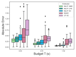
Figure 1: Boundary-value ODE: Absolute integration error under a budget constraint.

To compare MCLF using quasi-Monte Carlo points (QMC), Latin hypercube sampling (LHS), and i.i.d points (IID) with MLMC and CF using i.i.d points, we repeat the experiment 100 times. The sample size, evaluation cost at each level, and other details can be found in Appendix B. As shown in Figure 1, under the same evaluation cost constraint, MLCF outperforms MLMC and CF. Figure 1 also shows that experimental designs can improve the performance of MLCF.

Bayesian Inference for Lotka-Volterra

We now consider to perform Bayesian inference for the Lotka-Volterra system [Lotka, 1925, 1927, Volterra, 1927], which is also known as the predator-prey model. The model usually uses a system of differential equations:

$$\textstyle\frac{du_{1}(t)}{dt} \textstyle=x_{1}u_{1}(t)-x_{2}u_{1}(t)u_{2}(t),$$

$$\textstyle\frac{du_{2}(t)}{dt} \textstyle=x_{3}u_{1}(t)u_{2}(t)-x_{4}u_{2}(t),$$

to describe the interaction between a predator and its prey in an ecosystem. $u_{1}(t)$ and $u_{2}(t)$ are the prey population and the predator population at time $t\in[0,s]$, for some $s\in\mathbb{R}_{+}$. The initial conditions of the system are $u_{1}(0)=x_{5}$ and $u_{2}(0)=x_{6}$. The observations $u_{1}(t_{i})$ and $u_{2}(t_{i})$ obtained exhibit log-normal noise with independent standard deviation $x_{7}$ and $x_{8}$ respectively, for all $i\in\{1,\ldots,m\}$. We can re-parameterise $x$ as in Sun et al. [2021, 2023] such that the re-parameterised model has parameters $\tilde{x}\in\mathbb{R}^{8}$. With the Gaussian distribution priors we assign on $\tilde{x}$ and the observations, we can construct the posterior distribution of $\tilde{x}$. The quantity of interest $\Pi[f]$ is the posterior expectation of the average prey population over the time period between $0$ and $s$, i.e. $\Pi[f]=\int_{\mathbb{R}^{8}}f(\tilde{x})\pi(\tilde{x})d\tilde{x}$, where $\pi$ is the posterior probability distribution of $\tilde{x}$ and $f(\tilde{x})$ is the average prey population between $0$ and $s$ with the model parameter is $\tilde{x}$. $f(\tilde{x})=s^{-1}\int_{0}^{s}u_{1}(t)dt$ is approximated with $(s)^{-1}h\sum^{s/h}_{i=1}u_{1}(t_{i})$, where $h$ is the step size and each $u_{1}(t_{i})$ is obtained by solving the differential equations numerically. The real-world dataset [Hewitt, 1921] consisting of the population of snowshoe hares (prey) and Canadian lynxes (predators) is used as observations for our study. With the real-world observations, we conduct Bayesian inference and use a MCMC sampler (no-U-turn sampler) in Stan [Carpenter et al., 2017] to obtain samples.

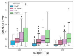
Figure 2: Bayesian Inference for Lotka-Volterra: Absolute integration error under a budget constraint.

We compare (i) MLCF with MCMC points, (ii) MLMC framework with MCMC points (MLMCMC), (iii) CF with MCMC points and (iv) MCMC. We repeat the experiment $50$ times. The sample size, sampling and evaluation cost at each level, and other details can be found in Appendix B. As shown in Figure 2, under the same budget constraint, MLCF outperforms all other methods.

5 Conclusion

In this initial work we introduced a generally applicable and efficient method for estimating intractable integrals, multilevel control function. The performance of the MLCF is demonstrated both theoretically, and empirically on an ODE example and a Bayesian inference for the Lotka-Volterra system. In the full version of this paper we will consider the optimal sample size at each level of MLCF and include an example based on the optimal sample size. This will allow us to optimize the performance of MLCF.

Appendix A Proofs

A.1 Proof of Proposition 1

Proof.

The unbiasedness can be obtained by taking the expectation with respect to the distribution $\Pi$ of the $n_{l}-m_{l}$ random variables that constitute $X^{1}_{l}$ for $l\in\{0,\ldots,L\}$. Firstly, we have that

$$\textstyle\mathbb{E}[k_{0}^{l}(X^{1}_{l},X^{0}_{l})k_{0}^{l}(X^{0}_{l},X^{0}_{l})^{-1}((f_{l}(X^{0}_{l})-f_{l-1}(X^{0}_{l}))-a_{l}\boldsymbol{1}_{m_{l}})]=0,$$

due to the property of the Stein kernel $k^{l}_{0}$ that the Stein kernel $k^{l}_{0}$ satisfies $\int_{\mathcal{X}}k^{l}_{0}(x,x^{\prime})\pi(x)dx=0$ for all $x\in\mathcal{X}$. Then, we have

$$\textstyle\mathbb{E}[\hat{\Pi}_{\textup{MLCF}}^{n-m}[f]] \textstyle:=\mathbb{E}[\sum^{L}_{l=0}\hat{\Pi}_{\textup{CF}}^{n-m}[f_{l}-f_{l-1}]]$$

$$\textstyle=\mathbb{E}[\sum^{L}_{l=0}\frac{1}{n_{l}-m_{l}}\boldsymbol{1}^{\top}\{(f_{l}(X^{1}_{l})-f_{l-1}(X^{1}_{l}))-k_{0}^{l}(X^{1}_{l},X^{0}_{l})k_{0}^{l}(X^{0}_{l},X^{0}_{l})^{-1}[(f_{l}(X^{0}_{l})-f_{l-1}(X^{0}_{l}))-a_{l}\boldsymbol{1}]\}]$$

$$\textstyle=[\sum^{L}_{l=0}\frac{1}{n_{l}-m_{l}}\boldsymbol{1}^{\top}\{\mathbb{E}[(f_{l}(X^{1}_{l})-f_{l-1}(X^{1}_{l}))]-\mathbb{E}\left[k_{0}^{l}(X^{1}_{l},X^{0}_{l})k_{0}^{l}(X^{0}_{l},X^{0}_{l})^{-1}[(f_{l}(X^{0}_{l})-f_{l-1}(X^{0}_{l}))-a_{l}\boldsymbol{1}]\right]\}]$$

$$\textstyle=\sum^{L}_{l=0}\Pi[f_{l}-f_{l-1}]$$

$$\textstyle=\Pi[f].$$

∎

A.2 Proof of Theorem 2

Proof.

Following the proof of Theorem 1 of [Oates et al., 2019] or Theorem 11.13 of [Wendland, 2004], under assumptions A1-7, there exists $C^{*}_{l}>0$ and $h^{*}_{l}>0$, for $h_{l}<h^{*}_{l}$,

$$\textstyle|f_{l}(x)-f_{l-1}(x)-s_{l}(x)|\leq C^{*}_{l}h_{l}^{\tau_{l}}\|f_{l}-f_{l-1}\|_{\mathcal{H}_{+}^{l}}$$

for all $x\in\mathcal{X}$. Since $X^{1}_{l}$ are i.i.d at each level, combing the bound above, we have

$$\textstyle\mathbb{V}_{X^{1}_{0},\ldots,X^{1}_{L}}[\hat{\Pi}_{\textup{MLCF}}[f]] \textstyle=\mathbb{V}_{X^{1}_{0},\ldots,X^{1}_{L}}[\sum_{l=0}^{L}\frac{1}{n_{l}-m_{l}}\sum_{i=m_{l}+1}^{n_{l}}\left(f_{l}(x_{(l,i)})-f_{l-1}(x_{(l,i)})-(s_{l}(x_{(l,i)})-\Pi[s_{l}])\right)]$$

$$\textstyle=\sum_{l=0}^{L}\frac{\mathbb{V}[f_{l}-f_{l-1}-s_{l}]}{n_{l}-m_{l}}$$

$$\textstyle=\sum_{l=0}^{L}\frac{\Pi[(f_{l}-f_{l-1}-s_{l})^{2}]-\Pi[f_{l}-f_{l-1}-s_{l}]^{2}}{n_{l}-m_{l}}$$

$$\textstyle\leq\sum_{l=0}^{L}\frac{\Pi[(f_{l}-f_{l-1}-s_{l})^{2}]}{n_{l}-m_{l}}$$

$$\textstyle=\sum_{l=0}^{L}\frac{\Pi[|f_{l}-f_{l-1}-s_{l}|^{2}]}{n_{l}-m_{l}}$$

$$\textstyle\leq\sum_{l=0}^{L}\frac{(C^{*}_{l}h_{l}^{\tau_{l}}\|f_{l}-f_{l-1}\|_{\mathcal{H}_{+}^{l}})^{2}}{n_{l}-m_{l}}.$$

Under the assumption A8, and let $C_{l}=qC^{*}_{l}$, we can then write

$$\textstyle\mathbb{V}_{X^{1}_{0},\ldots,X^{1}_{L}}[\hat{\Pi}_{\textup{MLCF}}[f]] \textstyle\leq\sum_{l=0}^{L}\frac{(qC^{*}_{l}m_{l}^{-\tau_{l}/d}\|f_{l}-f_{l-1}\|_{\mathcal{H}_{+}^{l}})^{2}}{n_{l}-m_{l}}$$

$$\textstyle=\sum_{l=0}^{L}\frac{(C_{l}m_{l}^{-\tau_{l}/d}\|f_{l}-f_{l-1}\|_{\mathcal{H}_{+}^{l}})^{2}}{n_{l}-m_{l}}.$$

∎

Appendix B Experimental Setup

In Section 4, the performance of MLCF is being evaluated through empirical assessments. We used different probability distributions in these experiments including Gaussian and intractable posterior distributions. Although some of the assumptions are not fulfilled in these experiments, we still use these examples to study the versatility of our method across a variety of settings. We used squared-exponential kernels in these examples.

For the ODE example, we have evaluation cost at each level $C=(C_{0},C_{1},C_{2})=(1.22,3.57,11.89)$ (all measured in $10^{-3}$ seconds). Under the same evaluation cost constraint, we compared (1) MLCF with Quasi-Monte Carlo points (QMC), (2) MLCF with Latin hypercube sampling (LHS), (3) MLCF with i.i.d points, (4) CF with i.i.d points, (5) MLMC with i.i.d points. The sample size is the optimal sample size for MLMC, which is listed in Table 1.

For the Lotka-Volterra example, we have sampling and evaluation cost at each level $C=(C_{0},C_{1},C_{2})=(6.88,34.41,165.18)$ (all measured in $10^{-4}$ seconds). We use different step sizes $h$ for different levels. Under the same budget constraint, we compare (1) MLCF with MCMC points, (2) MLMC framework with MCMC points (MLMCMC), (3) CF with MCMC points, (4) MCMC. The sample size is listed in Table 2.

Table 1: ODE example: Number of samples at level $l$ given budget constraint $T$.

T	$l=0$	$l=1$	$l=1$	CF
0.30 s	70	10	2	15
0.91s	209	31	5	45
1.52s	349	52	6	75

Table 2: Lotka-Volterra: Number of samples at level $l$ given budget constraint $T$.

T	$l=0$	$l=1$	$l=1$	CF	MCMC
0.26 s	207	23	2	20	20
0.51s	413	47	4	40	40
0.77s	620	70	6	60	60

References

• Anastasiou et al. [2023] A. Anastasiou, A. Barp, F-X. Briol, R. E. Ebner, B.and Gaunt, F. Ghaderinezhad, J. Gorham, A. Gretton, C. Ley, Q. Liu, et al. Stein’s method meets computational statistics: a review of some recent developments. Statistical Science, 38(1):120–139, 2023.
• Carpenter et al. [2017] Bob Carpenter, Andrew Gelman, Matthew D Hoffman, Daniel Lee, Ben Goodrich, Michael Betancourt, Marcus Brubaker, Jiqiang Guo, Peter Li, and Allen Riddell. Stan: A probabilistic programming language. Journal of statistical software, 76(1), 2017.
• Fairbanks et al. [2017] Hillary R Fairbanks, Alireza Doostan, Christian Ketelsen, and Gianluca Iaccarino. A low-rank control variate for multilevel Monte Carlo simulation of high-dimensional uncertain systems. Journal of Computational Physics, 341:121–139, 2017.
• Geraci et al. [2017] Gianluca Geraci, Michael S Eldred, and Gianluca Iaccarino. A multifidelity multilevel Monte Carlo method for uncertainty propagation in aerospace applications. In 19th AIAA non-deterministic approaches conference, page 1951, 2017.
• Giles [2008] Michael B Giles. Multilevel Monte Carlo path simulation. Operations research, 56(3):607–617, 2008.
• Giles [2015] Michael B Giles. Multilevel Monte Carlo methods. Acta numerica, 24:259–328, 2015.
• Hewitt [1921] Charles Gordon Hewitt. The conservation of the wild life of Canada. New York: C. Scribner, 1921.
• Li et al. [2023] Kaiyu Li, Daniel Giles, Toni Karvonen, Serge Guillas, and François-Xavier Briol. Multilevel Bayesian quadrature. In International Conference on Artificial Intelligence and Statistics, pages 1845–1868. PMLR, 2023.
• Lotka [1927] Alfred J Lotka. Fluctuations in the abundance of a species considered mathematically. Nature, 119(2983):12–12, 1927.
• Lotka [1925] Alfred James Lotka. Elements of physical biology. Williams & Wilkins, 1925.
• Nobile and Tesei [2015] Fabio Nobile and Francesco Tesei. A multilevel Monte Carlo method with control variate for elliptic PDEs with log-normal coefficients. Stochastic Partial Differential Equations: Analysis and Computations, 3:398–444, 2015.
• Oates et al. [2017] Chris J Oates, Mark Girolami, and Nicolas Chopin. Control functionals for Monte Carlo integration. Journal of the Royal Statistical Society: Series B (Statistical Methodology), 79(3):695–718, 2017.
• Oates et al. [2019] Chris J Oates, Jon Cockayne, François-Xavier Briol, and Mark Girolami. Convergence rates for a class of estimators based on Stein’s method. Bernoulli, 25(2):1141–1159, 2019.
• Peherstorfer et al. [2018] Benjamin Peherstorfer, Karen Willcox, and Max Gunzburger. Survey of multifidelity methods in uncertainty propagation, inference, and optimization. Siam Review, 60(3):550–591, 2018.
• Robert et al. [1999] Christian P Robert, George Casella, and George Casella. Monte Carlo statistical methods, volume 2. Springer, 1999.
• Si et al. [2022] Shijing Si, Chris Oates, Andrew B Duncan, Lawrence Carin, François-Xavier Briol, et al. Scalable control variates for Monte Carlo methods via stochastic optimization. In International Conference on Monte Carlo and Quasi-Monte Carlo Methods in Scientific Computing, pages 205–221. Springer, 2022.
• South et al. [2022] L. F. South, T. Karvonen, C. Nemeth, M. Girolami, and C. J. Oates. Semi-exact control functionals from Sard’s method. Biometrika, 2022.
• Sun et al. [2021] Zhuo Sun, Alessandro Barp, and François-Xavier Briol. Vector-valued control variates. arXiv preprint arXiv:2109.08944, 2021.
• Sun et al. [2023] Zhuo Sun, Chris J Oates, and François-Xavier Briol. Meta-learning control variates: Variance reduction with limited data. arXiv preprint arXiv:2303.04756, 2023.
• Volterra [1927] Vito Volterra. Variazioni e fluttuazioni del numero d’individui in specie animali conviventi, volume 2. Societá anonima tipografica" Leonardo da Vinci", 1927.
• Wan et al. [2019] R. Wan, M. Zhong, H. Xiong, and Z. Zhu. Neural control variates for variance reduction. ECML PKDD, page 533–547, 2019.
• Wendland [2004] Holger Wendland. Scattered data approximation, volume 17. Cambridge university press, 2004.