Multistatic Integrated Sensing and Communication System in Cellular Networks

Abstract

A novel multistatic multiple-input multiple-output (MIMO) integrated sensing and communication (ISAC) system in cellular networks is proposed. It can make use of widespread base stations (BSs) to perform cooperative sensing in wide area. This system is important since the deployment of sensing function can be achieved based on the existing mobile communication networks at a low cost. In this system, orthogonal frequency division multiplexing (OFDM) signals transmitted from the central BS are received and processed by each of the neighboring BSs to estimate sensing object parameters. A joint data processing method is then introduced to derive the closed-form solution of objects position and velocity. Numerical simulation shows that the proposed multistatic system can improve the position and velocity estimation accuracy compared with monostatic and bistatic system, demonstrating the effectiveness and promise of implementing ISAC in the upcoming fifth generation advanced (5G-A) and sixth generation (6G) mobile networks.

I Introduction

Sensing is one of the key techniques for the upcoming fifth generation advanced (5G-A) and sixth generation (6G) mobile networks [1]. Its current version focuses on the positioning of devices accessed to the network [2], [3]. This limits the usage of sensing in various scenarios with massive device-free sensing objects. To extend the application of sensing and enhance its capability, integrated sensing and communication (ISAC) system is recently proposed where the hardware, the spectrum and the waveform of communication are also utilized for sensing purpose [4], [5]. Therefore, considerable integration gain can be envisioned on cost, spectral efficiency and energy efficiency in ISAC systems. On the other hand, the sensing process needs to extract target parameters from the propagation channel while the communication process aims to correctly transfer the information via the channel [6], [7]. Hence, mutual benefits between sensing and communication may be achieved by fully exploiting results in both functions. These natural advantages make the deployment of ISAC system more desired in the existing mobile networks [8].

To construct a multiple-input multiple-output (MIMO) ISAC system, one simple approach is using a single base station (BS) as transceiver to sense the surrounding environment and this is referred to as monostatic sensing [9], [10]. By transmitting the communication signal, which is normally chosen as orthogonal frequency division multiplexing (OFDM) signal, the BS can receive the reflected signal from the sensing objects in the line-of-sight (LOS) scenario [11]. Then the object parameters, including position and radial velocity, can be obtained by estimating the angle of departure (AoD), angle of arrival (AoA), time delay and Doppler frequency shift, etc [12]. However, a full-duplex BS is required to accomplish the monostatic sensing, which is a currently immature technology [13]. In the existing mobile networks with time-division duplexing mode, an additional receiver can be implemented with physical isolation to the transmitter on the same BS while the size, cost and complexity of BSs are significantly increased. Moreover, the self-interference signal due to BS own transmission has much larger power than the reflected signal so that it has to be suppressed by digital cancellation technique [14]. Therefore, it is a great burden for the operators to deploy monostatic sensing in the mobile networks.

To address the issues in monostatic sensing, bistatic sensing utilizing two BSs is proposed [15], [16] where one BS acts as transmitter with the other one being receiver [17]. To estimate the parameters of objects, information of BS location is needed [18]. Owing to the long distance between BSs, self-interference is automatically addressed with no further hardware change necessary. Therefore, bistatic sensing is more promising for the practical implementation of ISAC. However, similar to the monostatic sensing, the bistatic sensing is unable to fully recover the information of velocity [18]. To overcome the challenges in both monostatic and bistatic sensing system, in this work we propose a novel multistatic ISAC system in cellular networks. In this system, multiple BSs are utilized to perform multistatic sensing where the sensing results of BS receivers can be jointly processed. It can also take advantages of the existing mobile networks to cover wide area and accelerate the deployment of sensing function. To the best of our knowledge, an analysis of the multistatic sensing in cellular networks is yet to be performed in the literature. The specific contributions of this work are:

1) Proposing a novel multistatic MIMO ISAC system in cellular networks. This system overcomes the challenges in monostatic and bistatic sensing and well satisfies the requirement of large-scale ISAC implementation for operators.

2) Proposing a low-complexity sensing method with joint data processing to estimate the position and velocity of sensing objects. A BS scheduling scheme is also provided.

3) Demonstrating the proposed multistatic ISAC system by simulating the root mean square error (RMSE) of position and velocity estimation. It is shown that the estimation accuracy in multistatic sensing can be improved when compared with monostatic and bistatic sensing system.

Organization: Section II formulates the multistatic ISAC system model in cellular networks. Section III descibes an efficient method to estimate the parameters of sensing objects. Section IV provides numerical simulation results to demonstrate effectiveness of the multistatic ISAC system. Section V concludes the work.

Notation: Bold lower and upper case letters denote vectors and matrices, respectively. Upper case letters in calligraphy denote sets. Letters not in bold font represent scalars. $\left|a\right|$ and $E\left[a\right]$ refer to the modulus and expectation of a scalar $a$. $\left[\mathbf{a}\right]_{i}$ and $\left\|\mathbf{a}\right\|$ refer to the $i$th element and $l_{2}-$norm of vector $\mathrm{\mathbf{a}}$, respectively. $\mathrm{\mathbf{A}}^{T}$, $\mathrm{\mathbf{A}}^{H}$, $\mathrm{\left[\mathbf{A}\right]}_{i,j}$ refer to the transpose, conjugate transpose, and $\left(i,j\right)$th entry of matrix $\mathrm{\mathbf{A}}$, respectively. $\mathbb{C}$ denotes the complex number set. $j=\sqrt{-1}$ denotes imaginary unit.

II System Model

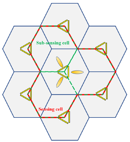
Figure 1: Illustration of sensing cell in multistatic ISAC system based on cellular network.

As depicted in Fig. 1, we consider a fragment of cellular network consisting of seven BSs where each BS has $3N$ antennas with every $N$ antennas cover a sector in its own cell. To perform multistatic sensing in this fragment, the central BS (referred to as transmitter) in Fig. 1 transmits signal to its surrounding environment in the downlink mode while the reflected signals from objects are received by $K=6$ BSs at the neighboring cells (referred to as receiver) in the uplink mode. Therefore, six sectors facing towards the central BS together with the central cell form a large multistatic sensing cell (referred to as sensing cell and enclosed by red line in Fig. 1). It should be noted that the structure of the sensing cell can be duplicated in any cellular network, making it simple to be widely deployed.

The multistatic MIMO sensing system can be decomposed onto multiple pairs of bistatic sensing system, then the time-domain system model with the $k$th receiver in the sensing cell can be written as

$$\mathbf{y}_{k}\left(t\right)= \stackrel{{\scriptstyle[}}{{l}}=1]{L}{\sum}\beta_{k,l}\delta\left(t-\tau_{k,l}\right)e^{j2\pi f_{D,k,l}t}\cdot$$

$$\mathbf{a}_{R,k}\left(\Omega_{R,k,l}\right)\mathbf{a}_{T}^{T}\left(\Omega_{T,l}\right)\mathbf{x}\left(t\right)+\mathbf{n}_{k}\left(t\right),\>k=1,2,...,K,$$ (1)

where $L$ is the number of sensing objects, $\beta_{k,l}\in\mathbb{C}$ is the channel gain of the $l$th path, $\delta\left(t\right)$ is the Dirac delta function and $\tau_{k,l}=\frac{d_{k,l}}{c}$ is the time delay with $d_{k,l}$ and $c$ referring to the signal propagation distance and light speed. Specifically, $d_{k,l}$ is given by $d_{k,l}=d_{T,l}+d_{R,k,l}$ where $d_{T,l}$ and $d_{R,k,l}$ are the propagation distance from the transmitter to the $l$th object and from the $l$th object to the $k$th receiver. $f_{D,k,l}=\frac{v_{\parallel,k,l}f_{c}}{c}$ is the Doppler frequency of the $l$th object with $v_{\parallel,k,l}$ and $f_{c}$ denoting radial velocity and carrier frequency respectively. In particular, $\hat{v}_{\parallel,k,l}=\hat{v}_{\parallel,R,k,l}+\hat{v}_{\parallel,T,l}$ where $\hat{v}_{\parallel,R,k,l}$ and $\hat{v}_{\parallel,T,l}$ are the radial velocity of the $l$th object with respect to the $k$th receiver and the transmitter [19]. $\mathbf{a}_{R,k}\left(\Omega_{R,k,l}\right)\in\mathbb{C}^{N\times 1}$ and $\mathbf{a}_{T}\left(\Omega_{T,l}\right)\in\mathbb{C}^{N\times 1}$ are the steering vectors of the receive antennas and the transmit antennas respectively, $\Omega_{R,k,l}=\left(\theta_{R,k,l},\phi_{R,k,l}\right)$ and $\Omega_{T,l}=\left(\theta_{T,l},\phi_{T,l}\right)$ are angle of arrival (AoA) and angle of departure (AoD) of the $l$th path with $\theta$ and $\phi$ representing the elevation and azimuth angles in spherical coordinates respectively. $\mathbf{x}\left(t\right)\in\mathbb{C}^{N\times 1}$ is the transmit signal and $\mathbf{y}_{k}\left(t\right)\in\mathbb{C}^{N\times 1}$ is the receive signal of the $k$th receiver. $\mathbf{n}_{k}\left(t\right)\in\mathbb{C}^{N\times 1}$ is the additive noise at the $k$th receiver.

For multistatic system with OFDM transmission scheme, we can demodulate the receive signal in the frequency domain by performing fast Fourier transform (FFT) on (1), then the receive OFDM symbol on the $n_{c}$th subcarrier ($n_{c}=0,1,...,N_{c}-1$ with $N_{c}$ being the total number of subcarriers) at the $n_{s}$th symbol period ($n_{s}=0,1,...,N_{s}-1$ with $N_{s}$ being the total number of OFDM symbols) is given by [6]

$$\tilde{\mathbf{y}}_{k}\left(f,t\right)\mid_{\begin{array}[]{c}f=n_{c}f_{\Delta}\\ t=n_{s}T_{s}\end{array}}= \stackrel{{\scriptstyle[}}{{l}}=1]{L}{\sum}\beta_{k,l}e^{j2\pi T_{s}f_{D,k,l}n_{s}}e^{-j2\pi\tau_{k,l}f_{\Delta}n_{c}}\cdot$$ (4)

$$\mathbf{a}_{R,k}\left(\Omega_{R,k,l}\right)\mathbf{a}_{T}^{T}\left(\Omega_{T,l}\right)\tilde{\mathbf{x}}\left(n_{c}f_{\Delta},n_{s}T_{s}\right)$$

$$+\tilde{\mathbf{n}}_{k}\left(n_{c}f_{\Delta},n_{s}T_{s}\right),\>k=1,2,...,K,$$ (5)

where $T_{s}$ is the OFDM symbol period, $f_{\Delta}$ is the subcarrier spacing, $\tilde{\mathbf{x}}$ is the transmit modulated symbols on subcarriers and $\tilde{\mathbf{n}}_{k}$ is the additive noise in frequency domain. It should be noted that to estimate the channel parameters related to the sensing objects, i.e. $f_{D,k,l}$, $\tau_{k,l}$, and $\Omega_{R,k,l}$, for $k=1,2,...,K$ and $l=1,2,...,L$, the transmit symbols $\tilde{\mathbf{x}}$ should be known at the receiver.

In this work, we consider the multistatic sensing on the azimuth plane ($\theta=90^{\circ}$) as an illustrative example to demonstrate our proposed system, which will be detailed in the following sections.

III Multistatic Sensing

In this section, we provide the solution of position and velocity of sensing objects in multistatic system. From operators’ perspective, conventional method such as multiple signal classification (MUSIC) [20] and estimating signal via rotational invariance techniques (ESPRIT) [21] algorithms are not preferred since eigenvalue decomposition in these methods cannot be efficiently processed by BS. Therefore, we propose a low-complexity method to estimate the channel parameters and derive the position as well as the velocity of sensing objects.

III-A Low-complexity Sensing Method

We start by estimating the AoA of receive signal in the time-domain (1). Assume the AoA remains unchanged within $N_{s}$ OFDM symbols period, we compensate (1) by using the steering vector of receive MIMO antenna array $\mathbf{a}_{R,k}\left(\phi\right)$ with angle variable $\phi$

$$g_{k}\left(\phi,t\right)=\mathbf{a}_{R,k}^{H}\left(\phi\right)\mathbf{y}_{k}\left(t\right),\>\phi\in\Phi{}_{k},\>t\in\left[0,N_{s}T_{s}\right]$$ (6)

where $\Phi{}_{k}$ is the angle range for the sector of the $k$th receiver in the sensing cell. Then we calculate the sum power of (6) at each angle during $N_{s}$ OFDM symbols period as

$$h_{k}\left(\phi\right)=\int_{0}^{N_{s}T_{s}}\left|g_{k}\left(\phi,t\right)\right|\mathrm{d}t.$$ (7)

Generally when $\phi=\phi_{R,k,l}$, $l=1,2,...,L$, the steering vector of receive antenna $\mathbf{a}_{R,k}\left(\phi\right)$ in (1) can be perfectly compensated so that (7) reaches local maximum value. Therefore, AoA $\hat{\phi}_{R,k}$ can be estimated by finding the peaks of $h_{k}\left(\phi\right)$ as

$$\hat{\Phi}_{R,k}=\left\{\hat{\phi}_{R,k}\mid h_{k}>\epsilon_{\phi},\frac{\mathrm{d}h_{k}}{\mathrm{d}\phi}=0,\frac{\mathrm{d^{2}}h_{k}}{\mathrm{d^{2}\phi}}<0\right\}$$ (8)

where $\epsilon_{\phi}$ is the threshold value which is related to the noise and interference power.

Next we estimate the time delay and radial velocity based on the receive OFDM symbols (5) and the estimated AoA. We firstly remove the information of transmit symbols $\tilde{\mathbf{x}}$ from the receive symbol $\tilde{\mathbf{y}}_{k}$. Specifically, the receive symbols $\tilde{\mathbf{y}}_{k}$ divided by the $i$th entry in $\tilde{\mathbf{x}}$ is written as

$$\tilde{\mathbf{h}}_{k,i}\left(n_{s},n_{c}\right)=\frac{\tilde{\mathbf{y}}_{k}}{\left[\tilde{\mathbf{x}}\right]_{i}}= \stackrel{{\scriptstyle[}}{{l}}=1]{L}{\sum}\beta_{k,l}e^{j2\pi T_{s}f_{D,k,l}n_{s}}e^{-j2\pi\tau_{k,l}f_{\Delta}n_{c}}\cdot$$

$$\left[\mathbf{a}_{T}\left(\phi_{T,l}\right)\right]_{i}\mathbf{a}_{R,k}\left(\phi_{R,k,l}\right)+\bar{\mathbf{n}}_{k,i},$$

$$k=1,2,...,K,\>i=1,2,...,N,$$ (9)

where $\left[\mathbf{a}_{T}\left(\phi_{T,l}\right)\right]_{i}$ in $\tilde{\mathbf{h}}_{k,i}\in\mathbb{C}^{N\times 1}$ can be combined into channel gain $\beta_{k,l}$. Then by compensating (9) with the steering vector of receive antenna for each angle in $\hat{\Phi}_{R,k}$, we have

$$\tilde{g}_{k,i}\left(n_{s},n_{c}\right)= \mathbf{a}_{R,k}^{H}\left(\phi\right)\tilde{\mathbf{h}}_{k,i}\left(n_{s},n_{c}\right),\>\phi\in\hat{\Phi}_{R,k},$$ (10)

where $\tilde{g}_{k,i}$ is a function of subcarrier index and symbol index on which we can perform two dimension (2D) discrete Fourier transform (DFT) [22]

$$\mathbf{G}_{k,i}\left(n_{s},n_{c}\right)= \mathbf{F}\tilde{g}_{k,i}\left(n_{s},n_{c}\right),\>i=1,2,...,N,$$ (11)

where $\mathbf{F}\in\mathbb{C}^{N_{s}\times N_{c}}$ is the 2D-DFT matrix with $\left[\mathbf{F}\right]_{p,q}=\frac{1}{N_{c}N_{s}}e^{-j\left(p-\frac{N_{s}}{2}\right)\frac{2\pi}{N_{s}}n_{s}}e^{j\left(q-1\right)\frac{2\pi}{N_{c}}n_{c}}$ ($N_{s}$ is assumed to be even). By taking (10) into (11), the phase brought by time delay and radial velocity can be offset when

$$T_{s}f_{D}=\frac{\left(\hat{p}_{k,i}-\frac{N_{s}}{2}\right)}{N_{s}}.$$ (12)

$$\tau f_{\Delta}=\frac{\left(\hat{q}_{k,i}-1\right)}{N_{c}},$$ (13)

where $\left(\hat{p}_{k,i},\hat{q}_{k,i}\right)$ is the index of peak in $\mathbf{G}_{k,i}$. It should be noted that the steps from (9) to (13) are the same for each transmit OFDM stream $i=1,2,...,N$ so that we define average peak index $\left(\hat{p}_{k},\hat{q}_{k}\right)=\frac{1}{N}\stackrel{{\scriptstyle[}}{{i}}=1]{N}{\sum}\left(\hat{p}_{k,i},\hat{q}_{k,i}\right)$ as the estimated peak index. The propagation distance $d$ and radial velocity $v_{\parallel}$ of the objects can then be solved as

$$\hat{v}_{\parallel,k}=\frac{\left(\hat{p}_{k}-\frac{N_{s}}{2}\right)c}{N_{s}T_{s}f_{c}},$$ (14)

$$\hat{d}_{k}=\frac{\left(\hat{q}_{k}-1\right)c}{N_{c}f_{\Delta}}.$$ (15)

By finding all peaks in $\mathbf{G}_{k,i}$ for each of the given angle in $\hat{\Phi}_{R,k}$, the estimated channel parameters of all sensing objects $\left(\hat{\phi}_{R,k},\hat{d}_{k},\hat{v}_{\parallel,k}\right)$ can be obtained.

We also provide here brief expressions of the estimation error on $\left(\hat{\phi}_{R,k},\hat{d}_{k},\hat{v}_{\parallel,k}\right)$. For the estimation of AoA, the error $\phi^{e}=\left|\hat{\phi}_{R,k}-\phi_{R,k}\right|$ depends on step size of $\phi$, denoted by $\Delta\phi$, and can be given by $E\left[\phi^{e}\right]=\frac{\Delta\phi}{4}$. This is because $\phi^{e}$ is uniformly distributed within $\left[0,\frac{\Delta\phi}{2}\right]$. Similarly, the resolution of radial velocity and propagation distance are respectively given by $\Delta v_{\parallel}=\frac{c}{N_{s}T_{s}f_{c}}$ and $\Delta d=\frac{c}{N_{c}f_{\Delta}}$. Therefore, the estimation error are written as $E\left[v_{\parallel}^{e}\right]=\frac{c}{4N_{s}T_{s}f_{c}}$ and $E\left[d^{e}\right]=\frac{c}{4N_{c}f_{\Delta}}$ which are inversely proportional to the total OFDM symbol period $N_{s}T_{s}$ and system bandwidth $N_{c}f_{\Delta}$ respectively.

III-B Position and Velocity Estimation

In this subsection, we derive the closed-form solution of position and velocity for sensing objects based on the estimation of AoA $\hat{\phi}_{R,k}$, propagation distance $\hat{d}_{k}$ and radial velocity $\hat{v}_{\parallel,k}$ of multiple receivers.

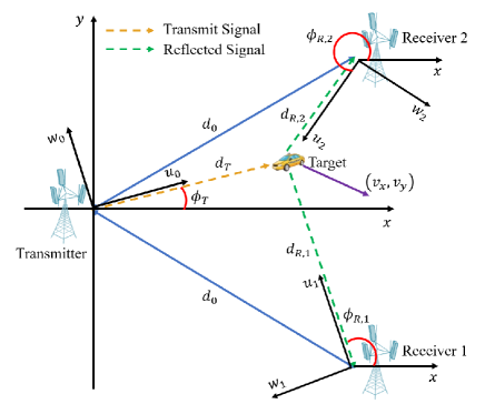
Figure 2: Illustration of position and velocity estimation.

Assume the coordinate of transmitter is $\left(x_{0},y_{0}\right)$ and the distance between the transmitter and receiver is $d_{0}$, then the location of receivers are given by $\left(x_{k},y_{k}\right)=\left(x_{0}+d_{0}\mathrm{cos}\left(\frac{2k\pi-1}{K}\right),y_{0}+d_{0}\mathrm{sin}\left(\frac{2k\pi-1}{K}\right)\right)$ for $k=1,2,...,K$. Utilizing the Law of Cosines together with AoA $\hat{\phi}_{R,k}$ and propagation distance $\hat{d}_{k}$, the distance between the object and $k$th receiver can be derived as

$$\hat{d}_{R,k}=\frac{\hat{d}_{k}^{2}-d_{0}^{2}}{2\left(\hat{d}_{k}+d_{0}\mathrm{cos}\left(\frac{2k\pi-1}{K}-\hat{\phi}_{R,k}\right)\right)}.$$ (16)

Therefore, the position of the object estimated by the $k$th receiver is given by

$$\hat{x}_{k}=x_{k}+\hat{d}_{R,k}\mathrm{cos}\left(\hat{\phi}_{R,k}\right),$$ (17)

$$\hat{y}_{k}=y_{k}+\hat{d}_{R,k}\mathrm{sin}\left(\hat{\phi}_{R,k}\right),$$ (18)

which are sent to server for joint data processing. In the single object case, the mean position can be obtained by averaging the position estimation results from multiple receivers as

$$\left(\hat{x},\hat{y}\right)=\frac{1}{K}\stackrel{{\scriptstyle[}}{{k}}=1]{K}{\sum}\left(\hat{x}_{k},\hat{y}_{k}\right).$$ (19)

Meanwhile, the estimated AoD is given by

$$\hat{\phi}_{T}=\mathrm{arctan}\left(\frac{\hat{y}-y_{0}}{\hat{x}-x_{0}}\right).$$ (20)

It should be noted that deriving the position of object by using two estimated AoA from two receivers cannot be applied in the scenario with multiple objects since the server is unable to properly match multiple AoAs from different receivers without additional information. In this scenario, clustering the position estimation results from different receivers based on the minimum Euclidean distance should be firstly performed. The mean position of sensing objects are then obtained by (19) for each cluster.

Next we derive the velocity of sensing objects based on the estimation results of AoA $\hat{\phi}_{R,k}$, AoD $\hat{\phi}_{T}$ and radial velocity $\hat{v}_{\parallel,k}$. As shown in Fig. 2, we set up local coordinate $\left(u,w\right)$ with the origin being the position of transmitter or receiver and the positive $u$-axis pointing from the origin to the object. The coordinate transformation from global coordinate $\left(x,y\right)$ to local coordinate $\left(u,w\right)$ can be expressed by matrix

$$\mathbf{T}\left(\hat{\phi}\right)=\left[\begin{array}[]{cc}\mathrm{cos}\left(\hat{\phi}\right)&\mathrm{sin}\left(\hat{\phi}\right)\\ -\mathrm{sin}\left(\hat{\phi}\right)&\mathrm{cos}\left(\hat{\phi}\right)\end{array}\right].$$ (21)

Then the velocity in global coordinate and in local coordinate for the $k$th receiver and the transmitter are respectively related by

$$\left[\begin{array}[]{c}\hat{v}_{\parallel,R,k}\\ \hat{v}_{\perp,R,k}\end{array}\right]=\mathbf{T}\left(\hat{\phi}_{R,k}\right)\left[\begin{array}[]{c}\hat{v}_{x}\\ \hat{v}_{y}\end{array}\right],$$ (22)

$$\left[\begin{array}[]{c}\hat{v}_{\parallel,T}\\ \hat{v}_{\perp,T}\end{array}\right]=\mathbf{T}\left(\hat{\phi}_{T}\right)\left[\begin{array}[]{c}\hat{v}_{x}\\ \hat{v}_{y}\end{array}\right],$$ (23)

where $\hat{v}_{x}$ and $\hat{v}_{y}$ are estimated velocity of object in the $x$-axis and $y$-axis direction in global coordinate, $\hat{v}_{\perp,R,k}$ and $\hat{v}_{\perp,T}$ are the normal velocity with respect to the $k$th receiver and the transmitter. By taking $\hat{v}_{\parallel,R,k}$ and $\hat{v}_{\parallel,T}$ in (22) and (23) into (14) we have

$$\hat{v}_{\parallel,k}= \left(\mathrm{cos}\left(\hat{\phi}_{R,k}\right)+\mathrm{cos}\left(\hat{\phi}_{T}\right)\right)\hat{v}_{x}$$

$$+\left(\mathrm{sin}\left(\hat{\phi}_{R,k}\right)+\mathrm{sin}\left(\hat{\phi}_{T}\right)\right)\hat{v}_{y}$$ (24)

To solve $\hat{v}_{x}$ and $\hat{v}_{y}$, at least two radial velocity results, denoted as $\hat{v}_{\parallel,k_{1}}$ and $\hat{v}_{\parallel,k_{2}}$, estimated from the $k_{1}$th and $k_{2}$th ($k_{1}\neq k_{2}$) receivers are required to perform joint processing. Alternatively, $\mathrm{sin}\left(\hat{\phi}_{T}\right)$ and $\mathrm{cos}\left(\hat{\phi}_{T}\right)$ in (24) can be canceled out by using three radial velocity results for the derivation of $\hat{v}_{x}$ and $\hat{v}_{y}$, which can avoid the usage of AoD estimation results. Therefore, the velocity of sensing objects can be fully recovered in the multistatic system.

III-C BS Scheduling Scheme

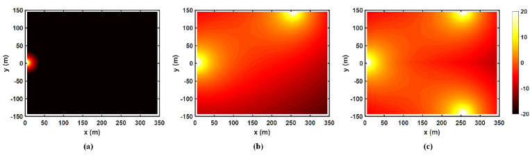
Figure 3: Simulated results relating the receive SNR to the object position in (a) monostatic, (b) bistatic and (c) multistatic sensing.

It can be noticed from the above analysis that multistatic sensing with two receivers provide enough information for obtaining the position as well as the velocity of sensing objects. In addition, the path gain is inversely proportional to the propagation distance square, which can be modeled as

$$\mathrm{PG}=\frac{\eta G_{T}G_{R}c^{2}}{\left(4\pi\right)^{3}d_{T}^{2}d_{R}^{2}f_{c}^{2}}$$ (25)

where $\eta$ is the radar cross-section (RCS) of sensing objects, $G_{T}$ and $G_{R}$ are the antenna gain of transmitter and receiver. Therefore, only the neighboring BSs with smallest $d_{R}$ can detect the reflected signal with significant power from the sensing objects. To avoid wasting BS resources, we discretize the sensing cell into three sub-sensing cells, each of which can be covered by two adjacent receivers as shown in Fig. 1 (enclosed by green dashed line). When sensing function is required in an area, two receivers in the corresponding sub-sensing cell are scheduled for sensing purpose. In this way, the maximum propagation distance in the sub-sensing cell is $2d_{0}$ when $d_{T}=d_{R}=d_{0}$ so that the $\mathrm{PG}$ can be always greater than $\frac{\eta G_{T}G_{R}c^{2}}{\left(4\pi\right)^{3}d_{0}^{4}f_{c}^{2}}$ which is associated with the minimum receive signal power.

IV Numerical Simulation

In the numerical simulation, multistatic sensing system in a sub-sensing cell as shown in Fig. 1 is considered. To evaluate its performance in position and velocity estimation, we assume a single sensing object locating in the sub-sensing cell. The range of object velocity is assumed to be $\left|v\right|\in\left[0,30\right]$ with arbitrary direction. We consider the carrier frequency of $f_{c}=2.6$ GHz where subcarrier spacing is $f_{\Delta}=30$ kHz and the OFDM symbol period is $T_{s}=\frac{0.5}{14}\>\mathrm{ms}=0.0357$ ms. Besides, the number of transmit and receive antennas are $N=16$ with the total antenna gain being $G_{T}=G_{R}=12$ dB. The distance between the transmitter and receiver is assumed as $d_{0}=300$ m and the location of transmitter and two receivers in the sub-sensing cell are given by $\left(0,0\right)$ m, $\left(260,150\right)$ m and $\left(260,-150\right)$ m.

We define the signal-to-interference-plus-noise ratio (SINR) as

$$\mathrm{SNR}=\frac{\mathrm{PG}\cdot P_{T}}{N_{0}+I_{0}}$$ (26)

where $P_{T}$ is the transmit signal power, $N_{0}$ is the noise power given by $N_{0}=-174+10\mathrm{log_{10}}\mathrm{BW}+NF$ dBm with $NF$ denoting noise figure, $I_{0}$ is the power of self-interference signal defined as $I_{0}=\alpha P_{T}$ with $\alpha$ representing the coefficient of self-interference cancellation. In the simulation, we use $\alpha=-70$ dB for monostatic sensing and $\alpha=0$ for bistatic and multistatic sensing. The other parameters are as follows: $P_{T}=30$ dBm, $\eta=1$, and $NF=10$ dB.

From (25) and (26), we can notice that SNR is a function of both propagation distance and interference power. Considering that SNR is the key factor of the accuracy in channel parameter estimation and the resulting position as well as velocity estimation in Section III, we firstly make comparison on receive SNR between the proposed multistatic sensing and the monostatic & bistatic sensing. It should be noted again that in monostatic sensing, the transmitter also receives the reflected signal of sensing object. In Fig. 3, we plot the receive SNR when sensing object locates at various positions in the sub-sensing cell. It can be observed that in multistatic sensing system, the maximum SNR at the receiver maintains above $-10$ dB for arbitrary position of sensing objects. This is because two BSs can receive the reflected signal simultaneously and SNR is always high for at least one of them. We also notice that SNR in monostatic sensing degrades sharply due to the interference power and the increase of propagation distance while SNR in bistatic sensing also decreases obviously as the object moves away from the BSs. Therefore, our proposed multistatic sensing system can cover larger area based on the cellular networks when compared with monostatic and bistatic sensing.

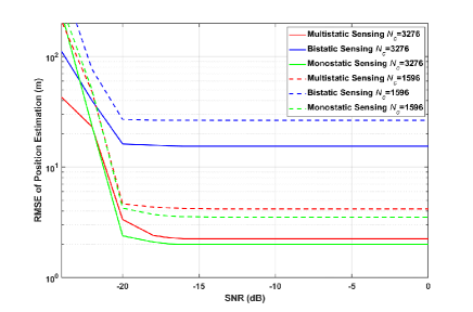
(a)

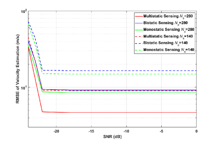
(b)

Figure 4: Simulated RMSE of (a) position and (b) velocity estimation in the proposed multistatic sensing system.

To further highlight the advantages of the proposed multistatic sensing system, we simulate the root mean square error (RMSE) of estimated position and velocity with respect to the actual values of sensing objects as shown in Fig. 4, which is also benchmarked with the performance of monostatic and bistatic sensing. For the position estimation in Fig. 4(a), we can make following observations: Firstly, it can be observed that the RMSE of positioning in multistatic sensing is smaller than that in bistatic sensing, which demonstrates the effectiveness of utilizing multiple receivers to improve the positioning accuracy. Secondly, the RMSE of positioning in multistatic sensing is slightly higher than that in monostatic sensing. This is because the estimation error on distance is reduced by half for the round-trip propagation in monostatic sensing, which is beneficial for the position estimation. However, combining with the results in Fig. 3, the multistatic sensing outperforms the monostatic sensing due to the high receive SNR for arbitrary object position. Thirdly, by comparing the results with different number of subcarriers $N_{c}$, we can notice that a larger system bandwidth can reduce the RMSE of position estimation.

We can also make several observations about the velocity estimation as shown in Fig. 4(b). It can be noticed that the RMSE of velocity estimation in multistatic sensing is much smaller than that in bistatic and monostatic sensing since bistatic and monostatic sensing can only provide the radial velocity of objects with significant error in terms of the normal velocity. Furthermore, The velocity estimation error in the multistatic sensing is related to the number of OFDM symbols $N_{s}$ where longer OFDM symbol period are desired for improving the velocity estimation accuracy.

To sum up, by using multistatic sensing in cellular network, the sensing area can be greatly expanded and both the position and velocity estimation accuracy can be significantly improved when compared with monostatic and bistatic sensing.

V Conclusions

In this paper, we propose a novel multistatic MIMO ISAC system in cellular networks. The proposed system well satisfies the ISAC implementation requirement of operators by making use of widely deployed BSs. Specifically in this system, the single transmit BS cooperates with multiple neighboring receive BSs whose sensing results are jointly processed to estimate the position and velocity of sensing objects. A BS scheduling scheme is also proposed to avoid wasting BS resources. It is shown by the numerical simulation that the proposed system can cover larger area and significantly reduce the position and velocity estimation error when compared with monostatic and bistatic sensing system, demonstrating the effectiveness of the proposed multistatic sensing and the promise of implementing such system in the upcoming 6G mobile networks.

This proposed system can serves as an initial guidance in ISAC deployment for operators. For future works, the design and the impact of beamforming at both transmitter and receiver side in multistatic sensing can be investigated. Beamforming at the transmitter can improve SNR by steering the main lobe to point to the sensing objects while the beamforming matrix is unknown to the receiver without additional notification. Therefore, the impact of unknown beamforming matrix on data decoding and channel parameters estimation requires further investigation.

References

- [1] F. Dong, F. Liu, Y. Cui, W. Wang, K. Han, and Z. Wang, “Sensing as a service in 6G perceptive networks: A unified framework for ISAC resource allocation,” IEEE Trans. Wirel. Commun., 2022.
- [2] J. Peisa, P. Persson, S. Parkvall, E. Dahlman, A. Grøvlen, C. Hoymann, and D. Gerstenberger, “5G evolution: 3GPP releases 16 & 17 overview,” Ericsson Technology Review, vol. 2020, no. 2, pp. 2–13, 2020.
- [3] X. Lin, “An overview of 5G advanced evolution in 3GPP release 18,” IEEE Commun. Stand. Mag., vol. 6, no. 3, pp. 77–83, 2022.
- [4] Y. Cui, F. Liu, X. Jing, and J. Mu, “Integrating sensing and communications for ubiquitous IoT: Applications, trends, and challenges,” IEEE Network, vol. 35, no. 5, pp. 158–167, 2021.
- [5] F. Liu, Y. Cui, C. Masouros, J. Xu, T. X. Han, Y. C. Eldar, and S. Buzzi, “Integrated sensing and communications: Towards dual-functional wireless networks for 6G and beyond,” IEEE J. Sel. Areas Commun., 2022.
- [6] J. A. Zhang, F. Liu, C. Masouros, R. W. Heath, Z. Feng, L. Zheng, and A. Petropulu, “An overview of signal processing techniques for joint communication and radar sensing,” IEEE J. Sel. Top. Signal Process., vol. 15, no. 6, pp. 1295–1315, 2021.
- [7] H. Hua, J. Xu, and T. X. Han, “Optimal transmit beamforming for integrated sensing and communication,” IEEE Trans. Veh. Technol., 2023.
- [8] A. Zhang, M. L. Rahman, X. Huang, Y. J. Guo, S. Chen, and R. W. Heath, “Perceptive mobile networks: Cellular networks with radio vision via joint communication and radar sensing,” IEEE Veh. Technol. Mag., vol. 16, no. 2, pp. 20–30, 2020.
- [9] S. Lu, F. Liu, and L. Hanzo, “The degrees-of-freedom in monostatic ISAC channels: NLoS exploitation vs. reduction,” IEEE Trans. Veh. Technol., 2022.
- [10] L. Pucci, E. Paolini, and A. Giorgetti, “System-level analysis of joint sensing and communication based on 5G new radio,” IEEE J. Sel. Areas Commun., vol. 40, no. 7, pp. 2043–2055, 2022.
- [11] C. B. Barneto, T. Riihonen, M. Turunen, L. Anttila, M. Fleischer, K. Stadius, J. Ryynänen, and M. Valkama, “Full-duplex OFDM radar with LTE and 5G NR waveforms: Challenges, solutions, and measurements,” IEEE Trans. Microwave Theory Tech., vol. 67, no. 10, pp. 4042–4054, 2019.
- [12] J.-F. Gu, J. Moghaddasi, and K. Wu, “Delay and Doppler shift estimation for OFDM-based radar-radio (RadCom) system,” in 2015 IEEE Int. Wirel. Symp. (IWS 2015). IEEE, 2015, pp. 1–4.
- [13] X. Wang, Z. Fei, J. A. Zhang, and J. Huang, “Sensing-assisted secure uplink communications with full-duplex base station,” IEEE Commun. Lett., vol. 26, no. 2, pp. 249–253, 2021.
- [14] S. Li and R. D. Murch, “An investigation into baseband techniques for single-channel full-duplex wireless communication systems,” IEEE Trans. Wirel. Commun., vol. 13, no. 9, pp. 4794–4806, 2014.
- [15] C. Cui, J. Xu, R. Gui, W.-Q. Wang, and W. Wu, “Search-free DOD, DOA and range estimation for bistatic FDA-MIMO radar,” IEEE Access, vol. 6, pp. 15 431–15 445, 2018.
- [16] L. Leyva, D. Castanheira, A. Silva, and A. Gameiro, “Two-stage estimation algorithm based on interleaved OFDM for a cooperative bistatic ISAC scenario,” in 2022 IEEE 95th Veh. Technol. Conf.:(VTC2022-Spring). IEEE, 2022, pp. 1–6.
- [17] L. Leyva, D. Castanheira, A. Silva, A. Gameiro, and L. Hanzo, “Cooperative multiterminal radar and communication: A new paradigm for 6G mobile networks,” IEEE Veh. Technol. Mag., vol. 16, no. 4, pp. 38–47, 2021.
- [18] L. Pucci, E. Matricardi, E. Paolini, W. Xu, and A. Giorgetti, “Performance analysis of a bistatic joint sensing and communication system,” in 2022 IEEE Int. Conf. Commun. Workshops (ICC Workshops). IEEE, 2022, pp. 73–78.
- [19] N. J. Willis, Bistatic radar. SciTech Publishing, 2005, vol. 2.
- [20] R. Schmidt, “Multiple emitter location and signal parameter estimation,” IEEE Trans. Antennas Propag., vol. 34, no. 3, pp. 276–280, 1986.
- [21] R. Roy and T. Kailath, “ESPRIT-estimation of signal parameters via rotational invariance techniques,” IEEE Trans. Acoust. Spe. Signal processing, vol. 37, no. 7, pp. 984–995, 1989.
- [22] C. Sturm and W. Wiesbeck, “Waveform design and signal processing aspects for fusion of wireless communications and radar sensing,” Proc. IEEE, vol. 99, no. 7, pp. 1236–1259, 2011.