Antithetic multilevel Monte Carlo method for approximations of SDEs with non-globally Lipschitz continuous coefficients 11footnotemark: 1

Chenxu Pang1, Xiaojie Wang1,22footnotemark: 2
1 School of Mathematics and Statistics, HNP-LAMA, Central South University, Changsha, Hunan, P. R. China
Abstract

In the field of computational finance, it is common for the quantity of interest to be expected values of functions of random variables via stochastic differential equations (SDEs). For SDEs with globally Lipschitz coefficients and commutative diffusion coefficients, the explicit Milstein scheme, relying on only Brownian increments and thus easily implementable, can be combined with the multilevel Monte Carlo (MLMC) method proposed by Giles [6] to give the optimal overall computational cost $\mathcal{O}(\epsilon^{-2})$, where $\epsilon$ is the required target accuracy. For multi-dimensional SDEs that do not satisfy the commutativity condition, a kind of one-half order truncated Milstein-type scheme without LΓ©vy areas is introduced by Giles and Szpruch [7], which combined with the antithetic MLMC gives the optimal computational cost under globally Lipschitz conditions. In the present work, we turn to SDEs with non-globally Lipschitz continuous coefficients, for which a family of modified Milstein-type schemes without LΓ©vy areas is proposed. The expected one-half order of strong convergence is recovered in a non-globally Lipschitz setting, where the diffusion coefficients are allowed to grow superlinearly. This helps us to analyze the relevant variance of the multilevel estimator and the optimal computational cost is finally achieved for the antithetic MLMC. The analysis of both the convergence rate and the desired variance in the non-globally Lipschitz setting is highly non-trivial and non-standard arguments are developed to overcome some essential difficulties. Numerical experiments are provided to confirm the theoretical findings.

AMS subject classification: 65C05, 60H15, 65C30.

Key Words: stochastic differential equations, modified Milstein scheme, non-globally Lipschitz condition, antithetic multilevel Monte Carlo

$$$$footnotetext: 11footnotemark: 1 This work was supported by Natural Science Foundation of China (12071488, 11971488) and Natural Science Foundation of Hunan Province (2020JJ2040). $$$$footnotetext: 22footnotemark: 2Corresponding author.
E-mail addresses: x.j.wang7@csu.edu.cn, c.x.pang@csu.edu.cn

1 Introduction

Throughout this paper, we consider ItΓ΄ stochastic differential equations (SDEs) as follows:

$$\left\{\begin{array}[]{l}\mathrm{d}X_{t}=\mu\left(X_{t}\right)\mathrm{d}t+\sigma\left(X_{t}\right)\mathrm{d}W_{t},\quad t\in(0,T]\\ X_{0}=x_{0},\end{array}\right.$$ (1.1)

where the drift coefficient function $\mu:\mathbb{R}^{d}\rightarrow\mathbb{R}^{d}$ and the diffusion coefficient function $\sigma:\mathbb{R}^{d}\rightarrow\mathbb{R}^{d\times m}$ are assumed to be non-globally Lipschitz continuous. Here $W_{\cdot}=\left(W_{1,\cdot},\dots,W_{m,\cdot}\right)^{T}:[0,T]\times\Omega\rightarrow\mathbb{R}^{m}$ denotes the $\mathbb{R}^{m}$-valued standard Brownian motion with respect to $\left\{\mathcal{F}_{t}\right\}_{t\in[0,T]}$ and the initial data $x_{0}:\Omega\rightarrow\mathbb{R}^{d}$ is assumed to be $\mathcal{F}_{0}$-measurable.

In recent years, SDEs have become a crucial instrument in a wide range of scientific fields and there has been, especially in computational finance, an increased emphasis on the quantification of expectations of some functions of the solution to SDEs (1.1). More accurately, one aims to compute

$$\mathbb{E}\left[\phi\left(X_{T}\right)\right]$$ (1.2)

for some given function $\phi$. To this end, the Monte Carlo (MC) method, combined with the Euler-Maruyama time-stepping scheme, is commonly used for this quantification at yet a high computational cost. Indeed, to achieve a root-mean-square error of $\epsilon$ of approximating the quantity (1.2), the computational cost will be $\mathcal{O}(\epsilon^{-3})$ [4].

Recently, a breakthrough was brought by Giles who generalized the multigrid idea in [17] and proposed the multilevel Monte Carlo (MLMC) method [6]. The MLMC method is regarded as a more effective algorithm with the aim to achieve a sharper bound for the mean-squared-error for a given computational cost. In the MLMC framework, some strongly convergent numerical scheme is used for the time discretization of SDEs (1.1) and the MC method is used to simulate a sequence of levels of approximations with different timestep sizes (see (2.2)). Evidently, higher level results in finer estimates but greater cost. The main idea to minimize the overall computational complexity of the MLMC is that more simulations are done on the lower level and relatively fewer simulations are needed on the upper level [6], leading to a significant reduction in the overall computational cost to $\mathcal{O}(\epsilon^{-2}(\log(1/\epsilon))^{2})$ when combined with the Euler-Maruyama discretization, and to $\mathcal{O}(\epsilon^{-2})$ when combined with the Milstein scheme for scalar SDEs [5]. Accordingly, the Milstein discretization with first-order strong convergence is superior in the case of dealing with scalar SDEs. This also holds true for SDEs with commutative diffusion coefficients, where the Milstein scheme relies on only Brownian increments.

However, for multi-dimensional SDEs that do not satisfy the commutativity condition, the Milstein scheme requires additional efforts to simulate the iterated ItΓ΄ integrals, also known as LΓ©vy areas (see (2.10)), which unavoidably reduces the efficiency of the scheme. So one may ask if any scheme with first-order strong convergence can be constructed without the LΓ©vy areas. Unfortunately, the authors of [3] give a negative answer and assert that $\mathcal{O}(h^{\frac{1}{2}})$ strong convergence is the best that can be achieved using only Brownian increments. Another natural question thus arises whether the optimal complexity $\mathcal{O}(\epsilon^{-2})$ can be achieved without the simulation of the LΓ©vy areas. By constructing a suitable antithetic estimator despite the $\mathcal{O}(h^{\frac{1}{2}})$ strong convergence, Giles and Szpruch [7] have very recently answered this question to the positive when both the drift and diffusion coefficients are assumed to be globally Lipschitz continuous.

What happens if the globally Lipschitz condition is violated? As asserted by [13], the basic Euler-Maruyama method using step-size $h>0$ fails to converge in a weak or strong sense in the asymptotic limit $h\rightarrow 0$ when used to solve SDEs with super-linearly growing coefficients. In [11], Hutzenthaler and Jentzen showed that the Monte Carlo combined with the Euler–Maruyama can achieve convergence almost surely in cases where the underlying Euler–Maruyama scheme diverges. This can happen when the events causing Euler–Maruyama to diverge are so rare that they are extremely unlikely to impact on any of the Monte Carlo samples (see [8] for relevant comments). However, as shown by [15], the MLMC method combined with the Euler–Maruyama scheme fails to converge to the desired quantity (1.2) for SDEs with super-linearly growing nonlinearities. In [15], a so-called tamed Euler was also shown to recover convergence in the multilevel setting. In other words, the MLMC method seems sensitive to the divergence of the numerical schemes and a strongly convergent numerical method for SDEs with non-globally Lipschitz continuous coefficients is necessary. Recent years have witnessed a growing interest in construction and analysis of convergent schemes in the non-globally Lipschitz setting (see [9, 12, 18, 19, 20, 22, 23, 25, 26, 27, 10] and references therein).

Nevertheless, for multidimensional SDEs whose coefficients do not obey the global Lipschitz condition, whether the antithetic MLMC method [7] can be adapted to achieve the optimal complexity $\mathcal{O}(\epsilon^{-2})$ is, as far as we know, still an unsolved problem. To solve this problem, we firstly propose strongly convergent Milstein-type methods without the LΓ©vy areas for SDEs (1.1) with non-commutative diffusion coefficients. More formally in this paper we establish a general framework for a family of modified Milstein (MM) scheme without LΓ©vy areas, given by

{Yn+1=𝒫​(Yn)+ΞΌh​(𝒫​(Yn))​h+Οƒh​(𝒫​(Yn))​Δ​Wn+βˆ‘j1,j2=1m(β„’j1​σj2)h​(𝒫​(Yn))​Πj1,j2tn,tn+1,Y0=x0,casessubscriptπ‘Œπ‘›1𝒫subscriptπ‘Œπ‘›subscriptπœ‡β„Žπ’«subscriptπ‘Œπ‘›β„ŽsubscriptπœŽβ„Žπ’«subscriptπ‘Œπ‘›Ξ”subscriptπ‘Šπ‘›superscriptsubscriptsubscript𝑗1subscript𝑗21π‘šsubscriptsuperscriptβ„’subscript𝑗1subscript𝜎subscript𝑗2β„Žπ’«subscriptπ‘Œπ‘›superscriptsubscriptΞ subscript𝑗1subscript𝑗2subscript𝑑𝑛subscript𝑑𝑛1subscriptπ‘Œ0subscriptπ‘₯0\left\{\begin{array}[]{l}Y_{n+1}=\mathscr{P}(Y_{n})+\mu_{h}\big{(}\mathscr{P}(Y_{n})\big{)}h+\sigma_{h}\big{(}\mathscr{P}(Y_{n})\big{)}\Delta W_{n}+\sum_{j_{1},j_{2}=1}^{m}\left(\mathcal{L}^{j_{1}}\sigma_{j_{2}}\right)_{h}\big{(}\mathscr{P}(Y_{n})\big{)}\Pi_{j_{1},j_{2}}^{t_{n},t_{n+1}},\\ Y_{0}=x_{0},\end{array}\right. (1.3)

where $h=\frac{T}{N}$, $N\in\mathbb{N}$, is the uniform timestep size, $\mathscr{P}:\mathbb{R}^{d}\rightarrow\mathbb{R}^{d}$ denotes some projection operator and $\mu_{h}(\cdot):\mathbb{R}^{d}\rightarrow\mathbb{R}^{d}$, $\sigma_{h}(\cdot):\mathbb{R}^{d}\rightarrow\mathbb{R}^{d\times m}$, $\left(\mathcal{L}^{j_{1}}\sigma_{j_{2}}\right)_{h}(\cdot):\mathbb{R}^{d}\rightarrow\mathbb{R}^{d}$, $j_{1},j_{2}\in\{1,\dots,m\}$, can be regarded as certain modifications to the coefficients $\mu,\sigma$ and $\mathcal{L}^{j_{1}}\sigma_{j_{2}}$ defined by (2.6). Moreover, we denote $\Delta W_{n}:=W_{t_{n+1}}-W_{t_{n}}$, $n\in\{0,1,\dots,N-1\}$, $\Delta W_{j,n}:=W_{j,t_{n+1}}-W_{j,t_{n}},j\in\{1,\dots,m\}$ and

Ξ j1,j2tn,tn+1:=12​(Δ​Wj1,n​Δ​Wj2,nβˆ’Ξ©j1​j2​h)withΞ©j1​j2={1,j1=j20,j1β‰ j2,j1,j2∈{1,…,m}.formulae-sequenceassignsuperscriptsubscriptΞ subscript𝑗1subscript𝑗2subscript𝑑𝑛subscript𝑑𝑛112Ξ”subscriptπ‘Šsubscript𝑗1𝑛Δsubscriptπ‘Šsubscript𝑗2𝑛subscriptΞ©subscript𝑗1subscript𝑗2β„Žwithformulae-sequencesubscriptΞ©subscript𝑗1subscript𝑗2cases1subscript𝑗1subscript𝑗20subscript𝑗1subscript𝑗2subscript𝑗1subscript𝑗21β€¦π‘š\Pi_{j_{1},j_{2}}^{t_{n},t_{n+1}}:=\tfrac{1}{2}\left(\Delta W_{j_{1},n}\Delta W_{j_{2},n}-\Omega_{j_{1}j_{2}}h\right)\quad\text{with}\quad\Omega_{j_{1}j_{2}}=\left\{\begin{array}[]{l}1,\quad j_{1}=j_{2}\\ 0,\quad j_{1}\neq j_{2}\end{array}\right.,\,j_{1},j_{2}\in\{1,\dots,m\}. (1.4)

Even neglecting the modifications to the coefficients and the projection operator, the proposed schemes (1.3), only relying on Brownian increments, are different from the classical Milstein scheme that involves the iterated ItΓ΄ integrals and can be viewed as a truncation version of the Milstein scheme. Such a truncation prevents the continuous-time extension of (1.3) from being an ItΓ΄ process and the ItΓ΄ formula is thus not applicable [21]. This is not an issue for the analysis in the globally Lipschitz setting but causes essential difficulties in the analysis of both the convergence rate, moment bounds and the relevant variance.

Indeed, when treating SDEs with superlinearly growing coefficients by explicit time-stepping schemes, it becomes a standard way in the literature to work with continuous-time extensions of the explicit schemes and carry out the analysis based on the ItΓ΄ formula (see, e.g., [23, 19, 14, 26]). In this work, non-standard arguments are developed to overcome these difficulties in the analysis. For example, to obtain high-order moments of the schemes, we work with the discrete scheme (1.3) and rely on discrete strategies based on Taylor expansions (see the proof of Theorem 4.1). In the analysis of the convergence order, by introducing an auxiliary process $\{\widetilde{Y}_{n}\}_{0\leq n\leq N}$, defined by

Y~n+1=Y~n+∫tntn+1μ​(Xs)​ds+∫tntn+1σ​(Xs)​dWs+βˆ‘j1,j2=1m(β„’j1​σj2)h​(𝒫​(Yn))​Πj1,j2tn,tn+1,Y~0=x0,formulae-sequencesubscript~π‘Œπ‘›1subscript~π‘Œπ‘›superscriptsubscriptsubscript𝑑𝑛subscript𝑑𝑛1πœ‡subscript𝑋𝑠differential-d𝑠superscriptsubscriptsubscript𝑑𝑛subscript𝑑𝑛1𝜎subscript𝑋𝑠differential-dsubscriptπ‘Šπ‘ superscriptsubscriptsubscript𝑗1subscript𝑗21π‘šsubscriptsuperscriptβ„’subscript𝑗1subscript𝜎subscript𝑗2β„Žπ’«subscriptπ‘Œπ‘›superscriptsubscriptΞ subscript𝑗1subscript𝑗2subscript𝑑𝑛subscript𝑑𝑛1subscript~π‘Œ0subscriptπ‘₯0\widetilde{Y}_{n+1}=\widetilde{Y}_{n}+\int_{t_{n}}^{t_{n+1}}\!\mu(X_{s})\ \mathrm{d}s+\int_{t_{n}}^{t_{n+1}}\!\sigma(X_{s})\ \mathrm{d}W_{s}+\sum_{j_{1},j_{2}=1}^{m}\!\left(\mathcal{L}^{j_{1}}\sigma_{j_{2}}\right)_{h}\big{(}\mathscr{P}(Y_{n})\big{)}\Pi_{j_{1},j_{2}}^{t_{n},t_{n+1}},\,\widetilde{Y}_{0}=x_{0}, (1.5)

we separate the strong error $\|X_{t_{n}}-Y_{n}\|_{L^{2p}(\Omega,\mathbb{R}^{d})}$ into two parts:

$$\|X_{t_{n}}-Y_{n}\|_{L^{2p}(\Omega,\mathbb{R}^{d})}\leq\|X_{t_{n}}-\widetilde{Y}_{n}\|_{L^{2p}(\Omega,\mathbb{R}^{d})}+\|\widetilde{Y}_{n}-Y_{n}\|_{L^{2p}(\Omega,\mathbb{R}^{d})}.$$ (1.6)

Here the first error item $\|X_{t_{n}}-\widetilde{Y}_{n}\|_{L^{2p}(\Omega,\mathbb{R}^{d})}$ can be directly and easily estimated (see the proof of Lemma 4.2). From (1.3) and (1.5), one can easily observe that $\widetilde{Y}_{n}-Y_{n}$ can be continuously extended to be an ItΓ΄ process and thus the remaining item $\|\widetilde{Y}_{n}-Y_{n}\|_{L^{2p}(\Omega,\mathbb{R}^{d})}$ can be estimated with the aid of the ItΓ΄ formula (see the proof of Lemma 4.5). Then a strong convergence rate of order $\tfrac{1}{2}$ is derived for the scheme (1.3).

Based on the numerical scheme (1.3) applied to discretize SDEs (1.1), we adopt the antithetic MLMC approach originally introduced by [7] to approximate the expectations and propose the antithetic MLMC-modified Milstein method to approximate $\mathbb{E}[\phi\left(X_{T}\right)]$ for SDEs with non-globally Lipschitz coefficiets. In order to show the optimal complexity, the key element is to derive the $\mathcal{O}(h^{\beta}),\beta>1$ variance of the multilevel estimator, in view of the well-known MLMC complexity theorem (see Theorem 2.1). However, this can not be achieved by trivially extending the analysis in [7] for a globally Lipschitz setting to the non-globally Lipschitz setting in this work. More precisely, some arguments used in [7] relying on the globally Lipschitz setting do not work in our setting. To address this issue, we employ the previously obtained one-half convergence order to arrive at a sub-optimal estimate $\mathbb{E}[\big{\|}\overline{Y}_{n}^{f}-Y_{n}^{c}\big{\|}^{2}]\leq Ch,$ which leads to the $\mathcal{O}(h)$ variance (see Lemma 5.4) first. Using this sub-optimal estimate and carrying out more careful error estimates on the mesh grids, we can improve the convergence rate to be order $1$, i.e., $\mathbb{E}[\big{\|}\overline{Y}_{n}^{f}-Y_{n}^{c}\big{\|}^{2}]\leq Ch^{2},$ and hence deduce the $\mathcal{O}(h^{2})$ variance as required (see Lemma 5.8).

The contribution of the present article can be summarized as follows: 1). A general framework of modified Milstein-type schemes without the LΓ©vy areas is established for SDEs with non-globally Lipschitz coefficients and the strong convergence rate is revealed under a coupled monotoncity condition and certain polynomial growth conditions. The framework covers the tamed Milstein scheme and projected Milstein scheme without LΓ©vy areas as special cases; 2). Combining the proposed schemes with the antithetic multilevel Monte Carlo we analyze the variance of the multilevel estimator and obtain the order two variance so that the optimal complexity $\mathcal{O}(\epsilon^{-2})$ can be derived. This justifies the use of antithetic MLMC combined with the MM scheme for SDEs with non-globally Lipschitz coefficients. As already mentioned above, the analysis of both the strong convergence rate and the desired variance is highly non-trivial and essential difficulties are caused by the non-globally Lipschitz setting, where the diffusion coefficients are allowed to grow polynomially.

The rest of this article is organized as follows. The next section revisits the fundamentals of antithetic MLMC for SDEs with globally Lipschitz drift and diffusion. In Section 3, we give the modified Milstein (MM) scheme and the main result of this article under a non-globally Lipschitz setting. Then the strong convergence analysis of our numerical method is presented in Section 4. In Section 5, we reveal the variance analysis of the multilevel estimator constructed by the MM scheme. Section 6 shows some numerical tests to illustrate our findings. Finally, the Appendix contains the detailed proof of several lemmas and theorems.

2 The antithetic MLMC revisited

The following setting is used throughout this paper. Let $\mathbb{N}$ be the set of all positive integers and $d,m\in\mathbb{N}$, $T\in(0,\infty)$ as given. Let $\|\cdot\|$ and $\langle\cdot,\cdot\rangle$ denote the Euclidean norm and the inner product of vectors in $\mathbb{R}^{d}$, respectively. With the same notation as for the vector norm, by $\|A\|:=\sqrt{\operatorname{trace}\left(A^{T}A\right)}$ we denote the trace norm of a matrix $A\in\mathbb{R}^{d\times m}$ and by $A^{T}\in\mathbb{R}^{m\times d}$ the transpose of a matrix $A\in\mathbb{R}^{d\times m}$. Let $(\Omega,\mathcal{F},\left\{\mathcal{F}_{t}\right\}_{t\in[0,T]},\mathbb{P})$ be a filtered probability space that satisfies the usual conditions. Also, we use $L^{r}\left(\Omega,\mathbb{R}^{d}\right),r\in\mathbb{N}$, to denote a family of $\mathbb{R}^{d}$-valued random variables $\xi$ satisfying $\mathbb{E}\left[\|\xi\|^{r}\right]<\infty$. For two real numbers $a$ and $b$, we denote $a\vee b=\max(a,b)$. In the following, we use $\frac{\partial\zeta}{\partial x}$ to denote the Jacobian matrix of the vector function $\zeta:\mathbb{R}^{d}\rightarrow\mathbb{R}^{d}$. For the real-valued function $\varphi:\mathbb{R}^{d}\rightarrow\mathbb{R}$, we use the same notation $\frac{\partial\varphi}{\partial x}$ to denote its gradient vector. Moreover, let $\textbf{1}_{D}$ be the indicative function of a set $D$ and let $C$ be a generic positive constant, which may be different for each appearance but is independent of the timestep.

In computational finance, it is common for the quantity of interest to be

$$\mathbb{E}[\phi\left(X_{T}\right)],$$

where $X_{T}$ is the solution of SDEs (1.1) at the final time $T$ and $\phi\in C_{b}^{2}(\mathbb{R}^{d},\mathbb{R})$ is some smooth payoff function with first and second bounded derivatives, i.e., $\big{\|}\tfrac{\partial\phi}{\partial x}\big{\|}\vee\big{\|}\tfrac{\partial^{2}\phi}{\partial x^{2}}\big{\|}<\infty.$ For simplicity, we denote

$$P:=\phi(X_{T}).$$ (2.1)

In addition, we denote $\hat{P}_{\ell}$ as the approximation of $P$ using a numerical discretization with timestep $h_{\ell}=\frac{T}{2^{\ell}}$, $\ell\geq 1$. For some $L>1$, the simulation of $\mathbb{E}[\hat{P}_{L}]$ can be split into a series of levels of resolutoin as

$$\mathbb{E}\big{[}\hat{P}_{L}\big{]}=\mathbb{E}\big{[}\hat{P}_{0}\big{]}+\sum_{\ell=1}^{L}\mathbb{E}\big{[}\hat{P}_{\ell}-\hat{P}_{\ell-1}\big{]}.$$ (2.2)

The idea behind MLMC is to independently estimate each of the expectations on the right-hand side of (2.2) in a way which minimises the overall variance for a given computational cost. Further, let ${Z}_{0}$ be an estimator of $\mathbb{E}[\hat{P}_{0}]$ with $N_{0}$ Monte Carlo samples and ${Z}_{\ell}$ be an estimator of $\mathbb{E}[\hat{P}_{\ell}-\hat{P}_{\ell-1}]$ with $N_{\ell}$ Monte Carlo samples, i.e.

$$Z_{\ell}=\left\{\begin{array}[]{ll}N_{0}^{-1}\sum_{i=1}^{N_{0}}\hat{P}_{0}^{(i)},&\ell=0,\\ N_{\ell}^{-1}\sum_{i=1}^{N_{\ell}}\left(\hat{P}_{\ell}^{(i)}-\hat{P}_{\ell-1}^{(i)}\right),&\ell>0.\end{array}\right.$$ (2.3)

Moreover, the final multilevel estimator $Z$ is given by the sum of the level estimators (2.3) as

$$Z=\sum_{\ell=0}^{L}Z_{\ell}.$$ (2.4)

The key point here is that $\hat{P}_{\ell}^{(i)}-\hat{P}_{\ell-1}^{(i)}$ should come from two discrete approximations for the same underlying stochastic sample, so that on finer levels of resolution the difference is small (due to strong convergence) and so the variance is also small. Hence very few samples will be required on finer levels to accurately estimate the expected value. Next we recall the MLMC complexity theorem in [6].

Theorem 2.1.

Let $P$, $Z_{\ell}$ and $Z$ be defined as (2.1), (2.3) and (2.4), respectively. Let $P_{\ell}$ be the corresponding level $\ell$ numerical approximation. If there exists positive constants $\alpha$, $\beta$, $\theta$, $c_{1}$, $c_{2}$, $c_{3}$ such that $\alpha\geq\frac{1}{2}\min\{\beta,\theta\}$ and:

$\displaystyle\text{ (i) }\left|\mathbb{E}\big{[}\hat{P}_{\ell}-P\big{]}\right|\leq c_{1}h_{\ell}^{\alpha},$
$\displaystyle\text{ (ii) }\mathbb{E}\left[Z_{\ell}\right]=\left\{\begin{array}[]{ll}\mathbb{E}\big{[}\hat{P}_{0}\big{]},&\ell=0\\ \mathbb{E}\big{[}\hat{P}_{\ell}-\hat{P}_{\ell-1}\big{]},&\ell>0\end{array}\right.$
$\displaystyle\text{ (iii) }\text{Var}\left[Z_{\ell}\right]\leq c_{2}N_{\ell}^{-1}h_{\ell}^{\beta},$
$\displaystyle\text{ (iv) }\mathcal{C}_{\ell}\leq c_{3}N_{\ell}h_{\ell}^{-\theta},$

where $\mathcal{C}_{\ell}$ is the computational complexity of $Z_{\ell}$. Then there exists a positive constant $c_{4}$ such that for any $\epsilon<e^{-1}$ there are values $L$ and $N_{\ell}$   for which the multilevel estimator (2.4) has a mean-square-error with bound

$$MSE\equiv\mathbb{E}\left[(Z-\mathbb{E}[P])^{2}\right]<\epsilon^{2}$$

with a computational complexity $\mathcal{C}$ with bound

$$\mathcal{C}\leq\left\{\begin{array}[]{ll}c_{4}\epsilon^{-2},&\beta>\theta\\ c_{4}\epsilon^{-2}(\log(1/\epsilon))^{2},&\beta=\theta\\ c_{4}\epsilon^{-2-(\theta-\beta)/\alpha},&0<\beta<\theta.\end{array}\right.$$

Usually, $\theta=1$ and as indicated by Theorem 2.1, the case $\beta>\theta=1$ can promise the optimal computational complexity $O(\epsilon^{-2})$. Note that the strong Euler-type scheme gives one-half order of strong convergence and thus $\beta=\theta=1$. However, the Milstein scheme has strong convergence rate of order $1$ so that $\beta=2>\theta=1$ and the optimal computational complexity can be obtained.

For the underlying SDEs (1.1), the classical Milstein scheme $\{\hat{X}_{n}\}_{0\leq n\leq N}$ using a uniform timestep $h=\frac{T}{N}$, $N\in\mathbb{N}$, takes the following form:

$$\left\{\begin{array}[]{ll}\hat{X}_{n+1}&=\hat{X}_{n}+\mu(\hat{X}_{n})h+\sigma(\hat{X}_{n})\Delta W_{n}+\sum_{j_{1},j_{2}=1}^{m}\left(\mathcal{L}^{j_{1}}\sigma_{j_{2}}\right)(\hat{X}_{n})\int^{t_{n+1}}_{t_{n}}\int^{s_{2}}_{t_{n}}\text{d}W_{s_{1}}^{j_{1}}\text{d}W_{s_{2}}^{j_{2}}\\ \hat{X}_{0}&=x_{0},\end{array}\right.$$ (2.5)

where $\Delta W_{n}:=W_{t_{n+1}}-W_{t_{n}}$, $n\in\{0,1,2,\ldots,N-1\}$, and the vector function $\mathcal{L}^{j_{1}}\sigma_{j_{2}}:\mathbb{R}^{d}\rightarrow\mathbb{R}^{d}$ is defined by

$$\mathcal{L}^{j_{1}}\sigma_{j_{2}}(x):=\sum_{k=1}^{d}\sigma_{k,j_{1}}\tfrac{\partial\sigma_{j_{2}}(x)}{\partial x^{k}}=\tfrac{\partial\sigma_{j_{2}}}{\partial x}(x)\sigma_{j_{1}}(x),\quad x\in\mathbb{R}^{d},\quad j_{1},j_{2}\in\{1,\dots,m\}.$$ (2.6)

Equivalently, the Milstein scheme can be rewritten as

{X^n+1=X^n+μ​(X^n)​h+σ​(X^n)​Δ​Wn+βˆ‘j1,j2=1m(β„’j1​σj2)​(X^n)​(Ξ j1,j2tn,tn+1+Lj1,j2tn,tn+1)X^0=x0,casessubscript^𝑋𝑛1absentsubscript^π‘‹π‘›πœ‡subscript^π‘‹π‘›β„ŽπœŽsubscript^𝑋𝑛Δsubscriptπ‘Šπ‘›superscriptsubscriptsubscript𝑗1subscript𝑗21π‘šsuperscriptβ„’subscript𝑗1subscript𝜎subscript𝑗2subscript^𝑋𝑛superscriptsubscriptΞ subscript𝑗1subscript𝑗2subscript𝑑𝑛subscript𝑑𝑛1superscriptsubscript𝐿subscript𝑗1subscript𝑗2subscript𝑑𝑛subscript𝑑𝑛1subscript^𝑋0absentsubscriptπ‘₯0\left\{\begin{array}[]{ll}\hat{X}_{n+1}&=\hat{X}_{n}+\mu(\hat{X}_{n})h+\sigma(\hat{X}_{n})\Delta W_{n}+\sum_{j_{1},j_{2}=1}^{m}\left(\mathcal{L}^{j_{1}}\sigma_{j_{2}}\right)(\hat{X}_{n})\left(\Pi_{j_{1},j_{2}}^{t_{n},t_{n+1}}+L_{j_{1},j_{2}}^{t_{n},t_{n+1}}\right)\\ \hat{X}_{0}&=x_{0},\end{array}\right. (2.7)

where the process Ξ j1,j2tn,tn+1superscriptsubscriptΞ subscript𝑗1subscript𝑗2subscript𝑑𝑛subscript𝑑𝑛1\Pi_{j_{1},j_{2}}^{t_{n},t_{n+1}} is given by

Ξ j1,j2tn,tn+1:=12​(Δ​Wj1,n​Δ​Wj2,nβˆ’Ξ©j1​j2​h),assignsuperscriptsubscriptΞ subscript𝑗1subscript𝑗2subscript𝑑𝑛subscript𝑑𝑛112Ξ”subscriptπ‘Šsubscript𝑗1𝑛Δsubscriptπ‘Šsubscript𝑗2𝑛subscriptΞ©subscript𝑗1subscript𝑗2β„Ž\Pi_{j_{1},j_{2}}^{t_{n},t_{n+1}}:=\tfrac{1}{2}\left(\Delta W_{j_{1},n}\Delta W_{j_{2},n}-\Omega_{j_{1}j_{2}}h\right), (2.8)

with $\Delta W_{j,n}:=W_{j,t_{n+1}}-W_{j,t_{n}}$ for $j\in\{1,\dots,m\}$ and for $j_{1},j_{2}\in\{1,\ldots,m\}$,

Ξ©j1​j2={1,j1=j2,0,j1β‰ j2.subscriptΞ©subscript𝑗1subscript𝑗2cases1subscript𝑗1subscript𝑗20subscript𝑗1subscript𝑗2\Omega_{j_{1}j_{2}}=\left\{\begin{array}[]{l}1,\quad j_{1}=j_{2},\\ 0,\quad j_{1}\neq j_{2}.\end{array}\right. (2.9)

Moreover, the term $L_{j_{1},j_{2}}^{t_{n},t_{n+1}}$ is the LΓ©vy area denoted as

$$L_{j_{1},j_{2}}^{t_{n},t_{n+1}}:=\int_{t_{n}}^{t_{n+1}}\left(W_{j_{1},t}-W_{j_{1},t_{n}}\right)\mathrm{d}W_{j_{2},t}-\int_{t_{n}}^{t_{n+1}}\left(W_{j_{2},t}-W_{j_{2},t_{n}}\right)\mathrm{d}W_{j_{1},t}.$$ (2.10)

For SDEs with commutative diffusion coefficients (i.e. $d=m=1$), the Milstein scheme (2.7), relying on only Brownian increments and thus easily implementable, can be combined with the multilevel Monte Carlo (MLMC) method to give $O(h^{2})$ variance in $(iii)$ of Theorem 2.1 (i.e., $\beta=2$) so that the optimal overall computational cost $\mathcal{O}(\epsilon^{-2})$ can be achieved [5]. However, for multi-dimensional SDEs without commutativity condition, to obtain the first order strong convergence, simulation of LΓ©vy areas (2.10) is unavoidable but expensive. Once setting (2.10) to be zero, the best strong convergence order of such a truncated Milstein method is $\frac{1}{2}$, which only gives $O(h)$ variance in $(iii)$ of Theorem 2.1 (i.e., $\beta=1$) and the overall computational cost is reduced to $\mathcal{O}(\epsilon^{-2}(\log(1/\epsilon))^{2})$. A natural question thus arises: can one obtain the optimal complexity without improving the strong convergence order of the numerical scheme?

To this end, one needs to exploit some flexibility in the construction of the multilevel estimator. Recall that the same estimator for $\hat{P}_{\ell}$ on every level $\ell$ is used in (2.3). However, Giles [5] numerically showed that it can be better to use different estimators for the finer and coarser of the two levels being considered, $\hat{P}_{\ell}^{f}$ when level $\ell$ is the finer level, and $\hat{P}_{\ell}^{c}$ when level $\ell$ is the coarser level. In this case we let $\hat{P}_{0}^{f}=\hat{P}_{0}^{c}$ and require

$$\mathbb{E}[\hat{P}_{\ell}^{f}]=\mathbb{E}[\hat{P}^{c}_{\ell}],\quad\ell=1,\dots,L,$$ (2.11)

so that the telescoping summation (2.2) remains valid and turns to be

$$\mathbb{E}\left[\hat{P}_{L}^{f}\right]=\mathbb{E}\left[\hat{P}_{0}^{f}\right]+\sum_{\ell=1}^{L}\mathbb{E}\left[\hat{P}_{\ell}^{f}-\hat{P}_{\ell-1}^{c}\right].$$ (2.12)

With this modified estimator, the MLMC complexity theorem (cf. Theorem 2.1) is still applicable and it gives the flexibility to construct approximations for which $\hat{P}_{\ell}^{f}-\hat{P}_{\ell-1}^{c}$ is much smaller than the original $\hat{P}_{\ell}-\hat{P}_{\ell-1}$, giving a larger rate $\beta$ of the relevant variance.

Following this idea, Giles and Szpruch [7] proposed an antithetic treatment which achieves the optimal complexity despite the $\frac{1}{2}$ strong convergence with globally Lipschitz coefficients. More precisely, using the coarser timestep $h\propto 2^{-\ell}$, the coarser path approximation $\{X^{c}\}$ is defined by a truncated Milstein method without LΓ©vy areas (i.e. set (2.10) to zero) as

Xn+1c=Xnc+μ​(Xnc)​h+σ​(Xnc)​Δ​Wn+βˆ‘j1,j2=1m(β„’j1​σj2)​(Xnc)​Πj1,j2tn,tn+1.subscriptsuperscript𝑋𝑐𝑛1subscriptsuperscriptπ‘‹π‘π‘›πœ‡subscriptsuperscriptπ‘‹π‘π‘›β„ŽπœŽsubscriptsuperscript𝑋𝑐𝑛Δsubscriptπ‘Šπ‘›superscriptsubscriptsubscript𝑗1subscript𝑗21π‘šsuperscriptβ„’subscript𝑗1subscript𝜎subscript𝑗2subscriptsuperscript𝑋𝑐𝑛superscriptsubscriptΞ subscript𝑗1subscript𝑗2subscript𝑑𝑛subscript𝑑𝑛1X^{c}_{n+1}=X^{c}_{n}+\mu(X^{c}_{n})h+\sigma(X^{c}_{n})\Delta W_{n}+\sum_{j_{1},j_{2}=1}^{m}\left(\mathcal{L}^{j_{1}}\sigma_{j_{2}}\right)(X^{c}_{n})\Pi_{j_{1},j_{2}}^{t_{n},t_{n+1}}. (2.13)

The finer approximation $\{X^{f}\}$ consists of two steps, first of which uses the same discretization as $\{X^{c}\}$ with time stepsize $\frac{h}{2}$,

Xn+1/2f=Xnf+μ​(Xnf)​h2+σ​(Xnf)​δ​Wn+βˆ‘j1,j2=1m(β„’j1​σj2)​(Xnf)​Πj1,j2tn,tn+1/2,subscriptsuperscript𝑋𝑓𝑛12subscriptsuperscriptπ‘‹π‘“π‘›πœ‡subscriptsuperscriptπ‘‹π‘“π‘›β„Ž2𝜎subscriptsuperscript𝑋𝑓𝑛𝛿subscriptπ‘Šπ‘›superscriptsubscriptsubscript𝑗1subscript𝑗21π‘šsuperscriptβ„’subscript𝑗1subscript𝜎subscript𝑗2subscriptsuperscript𝑋𝑓𝑛superscriptsubscriptΞ subscript𝑗1subscript𝑗2subscript𝑑𝑛subscript𝑑𝑛12X^{f}_{n+1/2}=X^{f}_{n}+\mu(X^{f}_{n})\tfrac{h}{2}+\sigma(X^{f}_{n})\delta W_{n}+\sum_{j_{1},j_{2}=1}^{m}\left(\mathcal{L}^{j_{1}}\sigma_{j_{2}}\right)(X^{f}_{n})\Pi_{j_{1},j_{2}}^{t_{n},t_{n+1/2}}, (2.14)

and the second of which reads

Xn+1f=Xn+1/2f+μ​(Xn+1/2f)​h2+σ​(Xnf)​δ​Wn+1/2+βˆ‘j1,j2=1m(β„’j1​σj2)​(Xn+1/2f)​Πj1,j2tn+1/2,tn+1,subscriptsuperscript𝑋𝑓𝑛1subscriptsuperscript𝑋𝑓𝑛12πœ‡subscriptsuperscript𝑋𝑓𝑛12β„Ž2𝜎subscriptsuperscript𝑋𝑓𝑛𝛿subscriptπ‘Šπ‘›12superscriptsubscriptsubscript𝑗1subscript𝑗21π‘šsuperscriptβ„’subscript𝑗1subscript𝜎subscript𝑗2subscriptsuperscript𝑋𝑓𝑛12superscriptsubscriptΞ subscript𝑗1subscript𝑗2subscript𝑑𝑛12subscript𝑑𝑛1X^{f}_{n+1}=X^{f}_{n+1/2}+\mu(X^{f}_{n+1/2})\tfrac{h}{2}+\sigma(X^{f}_{n})\delta W_{n+1/2}+\sum_{j_{1},j_{2}=1}^{m}\left(\mathcal{L}^{j_{1}}\sigma_{j_{2}}\right)(X^{f}_{n+1/2})\Pi_{j_{1},j_{2}}^{t_{n+1/2},t_{n+1}}, (2.15)

where

$$\delta W_{n}=W_{t_{n+1/2}}-W_{t_{n}},\quad\delta W_{n+1/2}=W_{t_{n+1}}-W_{t_{n+1/2}}.$$

The antithetic counterpart $\{X^{a}\}$ is defined by exactly the same discretization as $\{X^{f}\}$, with the exception that the Brownian increments $\delta W_{n}$ and $\delta W_{n+1/2}$ are swapped,

$\displaystyle X^{a}_{n+1/2}$ =Xna+μ​(Xna)​h2+σ​(Xna)​δ​Wn+1/2+βˆ‘j1,j2=1m(β„’j1​σj2)​(Xna)​Πj1,j2tn+1/2,tn+1,absentsubscriptsuperscriptπ‘‹π‘Žπ‘›πœ‡subscriptsuperscriptπ‘‹π‘Žπ‘›β„Ž2𝜎subscriptsuperscriptπ‘‹π‘Žπ‘›π›Ώsubscriptπ‘Šπ‘›12superscriptsubscriptsubscript𝑗1subscript𝑗21π‘šsuperscriptβ„’subscript𝑗1subscript𝜎subscript𝑗2subscriptsuperscriptπ‘‹π‘Žπ‘›superscriptsubscriptΞ subscript𝑗1subscript𝑗2subscript𝑑𝑛12subscript𝑑𝑛1\displaystyle=X^{a}_{n}+\mu(X^{a}_{n})\tfrac{h}{2}+\sigma(X^{a}_{n})\delta W_{n+1/2}+\sum_{j_{1},j_{2}=1}^{m}\left(\mathcal{L}^{j_{1}}\sigma_{j_{2}}\right)(X^{a}_{n})\Pi_{j_{1},j_{2}}^{t_{n+1/2},t_{n+1}}, (2.16)
$\displaystyle X^{a}_{n+1}$ =Xn+1/2a+μ​(Xn+1/2a)​h2+σ​(Xna)​δ​Wn+βˆ‘j1,j2=1m(β„’j1​σj2)​(Xn+1/2a)​Πj1,j2tn,tn+1/2.absentsubscriptsuperscriptπ‘‹π‘Žπ‘›12πœ‡subscriptsuperscriptπ‘‹π‘Žπ‘›12β„Ž2𝜎subscriptsuperscriptπ‘‹π‘Žπ‘›π›Ώsubscriptπ‘Šπ‘›superscriptsubscriptsubscript𝑗1subscript𝑗21π‘šsuperscriptβ„’subscript𝑗1subscript𝜎subscript𝑗2subscriptsuperscriptπ‘‹π‘Žπ‘›12superscriptsubscriptΞ subscript𝑗1subscript𝑗2subscript𝑑𝑛subscript𝑑𝑛12\displaystyle=X^{a}_{n+1/2}+\mu(X^{a}_{n+1/2})\tfrac{h}{2}+\sigma(X^{a}_{n})\delta W_{n}+\sum_{j_{1},j_{2}=1}^{m}\left(\mathcal{L}^{j_{1}}\sigma_{j_{2}}\right)(X^{a}_{n+1/2})\Pi_{j_{1},j_{2}}^{t_{n},t_{n+1/2}}. (2.17)

Further, we let

$$\hat{P}_{\ell}^{f}=\tfrac{1}{2}\big{(}\phi(X^{f}_{2^{\ell-1}})+\phi(X^{a}_{2^{\ell-1}})\big{)},\quad\hat{P}_{\ell-1}^{c}=\phi(X^{c}_{2^{\ell-1}}),\quad\ell=1,2,\dots,L.$$ (2.18)

As $\delta W_{n}$ and $\delta W_{n+1/2}$ are independent and identically distributed, $\{X^{a}\}$ has the same distribution as $\{X^{f}\}$ so that (2.11) can be easily checked. With the help of Theorem 2.1, Giles and Szpruch [7] deduced the optimal computational cost $\mathcal{O}(\epsilon^{-2})$ for the antithetic estimator they proposed under globally Lipschitz conditions, which is summarized as follows.

Theorem 2.2.

Let both drift and diffusion coefficients of SDE (1.1) be globally Lipschitz continuous with first and second uniformly bounded derivative. Let $P$, $\hat{P}^{f}_{\ell}$ and $\hat{P}^{c}_{\ell-1}$, $\ell=1,2,\dots,L$, be defined by (2.1) and (2.18). Moreover, let ${Z}_{0}$ be an estimator of $\mathbb{E}[\hat{P}^{f}_{0}]$ with $N_{0}$ Monte Carlo samples and ${Z}_{\ell}$ be an estimator of $\mathbb{E}[\hat{P}^{f}_{\ell}-\hat{P}^{c}_{\ell-1}]$ with $N_{\ell}$ Monte Carlo samples, i.e.

$$Z_{\ell}=\left\{\begin{array}[]{ll}N_{0}^{-1}\sum_{i=1}^{N_{0}}\hat{P}_{0}^{c,(i)},&\ell=0,\\ N_{\ell}^{-1}\sum_{i=1}^{N_{\ell}}\left(\hat{P}_{\ell}^{f,(i)}-\hat{P}_{\ell-1}^{c,(i)}\right),&\ell>0.\end{array}\right.$$ (2.19)

The final multilevel estimator $Z$ is given by

$$Z=\sum_{\ell=0}^{L}Z_{\ell}.$$ (2.20)

Then, there exists a positive constant $C$ such that

$$\text{Var}\big{[}Z_{\ell}\big{]}\leq CN_{\ell}^{-1}h^{2}_{\ell}.$$ (2.21)

Given the mean-square-error of $Z$ with bound

$$MSE\equiv\mathbb{E}\left[(Z-\mathbb{E}[P])^{2}\right]<\epsilon^{2},$$

there exists a constant $C$ such that the complexity $\mathcal{C}_{antitheticMLMC}$ has the bound

$$\mathcal{C}_{antitheticMLMC}\leq C\epsilon^{-2}.$$ (2.22)

In the forthcoming sections, we turn to SDEs with non-globally Lipschitz continuous coefficients and try to recover the above results in a non-globally Lipschitz setting. To this aim, we first need to introduce a modified and strongly convergent Milstein-type numerical scheme and later construct antithetic multilevel estimators following the same idea of [7]. However, the analysis for both the convergence rate and the desired variance is highly non-trivial and non-standard arguments are developed to overcome essential difficulties caused by the super-linearly growing coefficients.

3 Antithetic MLMC in a non-globally Lipschitz setting

In this section, we set up a non-globally Lipschitz framework by presenting some assumptions.

3.1 Settings and the modified Milstein scheme

We consider the following assumptions required to establish our main result.

Assumption 3.1.

(Coercivity condition) For some $p_{0}\geq 1$, there exists a positive constant $C$ such that

$$2\langle x,\mu(x)\rangle+(2p_{0}-1)\|\sigma(x)\|^{2}\leq C\left(1+\|x\|^{2}\right),\quad\forall x\in\mathbb{R}^{d}.$$ (3.1)
Assumption 3.2.

(A coupled monotoncity condition and globally polynomial growth conditions). Assume the drift coefficients $\mu:\mathbb{R}^{d}\rightarrow\mathbb{R}^{d}$ of the SDEs (1.1) are continuously differentiable and the diffusion coefficients $\sigma_{j}:\mathbb{R}^{d}\rightarrow\mathbb{R}^{d}$ are twice continuously differentiable. Moreover, there exist some positive constants $\gamma\in[1,\infty)$, $p_{1}\in(1,\infty)$, such that

$$2\langle x-\tilde{x},\mu(x)-\mu(\tilde{x})\rangle+(2p_{1}-1)\|\sigma(x)-\sigma(\tilde{x})\|^{2}\leq C\|x-\tilde{x}\|^{2},\quad\forall x,\tilde{x}\in\mathbb{R}^{d},$$ (3.2)

and for $j\in\{1,\ldots,m\}$,

$\displaystyle\left\|\left(\tfrac{\partial\mu}{\partial x}(x)-\tfrac{\partial\mu}{\partial x}(\tilde{x})\right)y\right\|$ $\displaystyle\leq C(1+\|x\|+\|\tilde{x}\|)^{\gamma-2}\|x-\tilde{x}\|\cdot\|y\|,\quad\forall x,\tilde{x},y\in\mathbb{R}^{d},\vspace{3ex}$ (3.3)
$\displaystyle\left\|\left(\tfrac{\partial\sigma_{j}}{\partial x}(x)-\tfrac{\partial\sigma_{j}}{\partial x}(\tilde{x})\right)y\right\|^{2}$ $\displaystyle\leq C(1+\|x\|+\|\tilde{x}\|)^{\gamma-3}\|x-\tilde{x}\|^{2}\cdot\|y\|^{2},\vspace{3ex}\quad\forall x,\tilde{x},y\in\mathbb{R}^{d}.$

Assume that the vector functions $\mathcal{L}^{j_{1}}\sigma_{j_{2}}:\mathbb{R}^{d}\rightarrow\mathbb{R}^{d},j_{1},j_{2}\in\{1,\ldots,m\}$ are continuously differentiable and

$$\left\|\left(\tfrac{\partial\left(\mathcal{L}^{j_{1}}\sigma_{j_{2}}\right)}{\partial x}(x)-\tfrac{\partial\left(\mathcal{L}^{j_{1}}\sigma_{j_{2}}\right)}{\partial x}(\tilde{x})\right)y\right\|\leq C\left(1+\|x\|+\|\tilde{x}\|\right)^{\gamma-2}\|x-\tilde{x}\|\cdot\|y\|,\quad\forall x,\tilde{x},y\in\mathbb{R}^{d}.$$ (3.4)

Further, the initial data $X_{0}$ is supposed to be $\mathcal{F}_{0}$-measurable, satisfying

$$\mathbb{E}\left[\left\|X_{0}\right\|^{2p_{0}}\right]<\infty,$$ (3.5)

where $p_{0}$ is determined by Assumption 3.1.

Assumption 3.2 is considered as a kind of polynomial growth condition and in proofs which follow we will need some implications of this assumption. It follows immediately that, for $j\in\{1,\ldots,m\}$,

$\displaystyle\left\|\tfrac{\partial\mu}{\partial x}(x)y\right\|\leq C(1+\|x\|)^{\gamma-1}\|y\|,\quad\forall x,y\in\mathbb{R}^{d},$ (3.6)
$\displaystyle\left\|\tfrac{\partial\sigma_{j}}{\partial x}(x)y\right\|^{2}\leq C(1+\|x\|)^{\gamma-1}\|y\|^{2},\quad\forall x,y\in\mathbb{R}^{d},$

which in turn gives

$\displaystyle\|\mu(x)-\mu(\tilde{x})\|$ $\displaystyle\leq C(1+\|x\|+\|\tilde{x}\|)^{\gamma-1}\|x-\tilde{x}\|,\quad\forall x,\tilde{x}\in\mathbb{R}^{d},$ (3.7)
$\displaystyle\|\mu(x)\|$ $\displaystyle\leq C(1+\|x\|)^{\gamma},\quad\forall x\in\mathbb{R}^{d},$

and, for $j_{1},j_{2}\in\{1,\ldots,m\}$,

$\displaystyle\left\|\sigma_{j}(x)-\sigma_{j}(\tilde{x})\right\|^{2}$ $\displaystyle\leq C(1+\|x\|+\|\tilde{x}\|)^{\gamma-1}\|x-\tilde{x}\|^{2},\quad\forall x,\tilde{x}\in\mathbb{R}^{d},$ (3.8)
$\displaystyle\|\sigma_{j}(x)\|^{2}$ $\displaystyle\leq C(1+\|x\|)^{\gamma+1},\quad\forall x\in\mathbb{R}^{d}.$

Similarly, (3.4) in Assumption 3.2 yields,

$\displaystyle\left\|\mathcal{L}^{j_{1}}\sigma_{j_{2}}(x)-\mathcal{L}^{j_{1}}\sigma_{j_{2}}(\tilde{x})\right\|$ $\displaystyle\leq C(1+\|x\|+\|\tilde{x}\|)^{\gamma-1}\|x-\tilde{x}\|,\quad\forall x,\tilde{x}\in\mathbb{R}^{d},$ (3.9)
$\displaystyle\left\|\mathcal{L}^{j_{1}}\sigma_{j_{2}}(x)\right\|$ $\displaystyle\leq C(1+\|x\|)^{\gamma},\quad\forall x\in\mathbb{R}^{d}.$

Note that Assumption 3.2 with Assumption 3.1 suffices to imply that SDE (1.1) possesses a unique $\{\mathcal{F}_{t}\}_{t\in[0,T]}$-adapted solution with continuous sample paths and

$$\mathbb{E}\left[\left\|X_{t}\right\|^{2p}\right]\leq C\left(1+\mathbb{E}\left[\left\|X_{0}\right\|^{2p}\right]\right)<\infty,\quad p\in[1,p_{0}],\quad t\in[0,T].$$ (3.10)

These assumptions cover a much broader class of SDEs than the globally Lipschitz condition. However, for the case that the coefficients of SDE (1.1) meet Assumption 3.1 and Assumption 3.2, the truncated Milstein schemes (2.13)-(2.15) and their antithetic version (2.16)-(2.17) may suffer from divergence, which results in the antithetic MLMC method being invalid. Throughout the paper, we propose a family of modified Milstein (MM) scheme on a uniform timestep $h=\frac{T}{N}$, $N\in\mathbb{N}$, given by

{Yn+1=𝒫​(Yn)+ΞΌh​(𝒫​(Yn))​h+Οƒh​(𝒫​(Yn))​Δ​Wn+βˆ‘j1,j2=1m(β„’j1​σj2)h​(𝒫​(Yn))​Πj1,j2tn,tn+1Y0=x0.casessubscriptπ‘Œπ‘›1𝒫subscriptπ‘Œπ‘›subscriptπœ‡β„Žπ’«subscriptπ‘Œπ‘›β„ŽsubscriptπœŽβ„Žπ’«subscriptπ‘Œπ‘›Ξ”subscriptπ‘Šπ‘›superscriptsubscriptsubscript𝑗1subscript𝑗21π‘šsubscriptsuperscriptβ„’subscript𝑗1subscript𝜎subscript𝑗2β„Žπ’«subscriptπ‘Œπ‘›superscriptsubscriptΞ subscript𝑗1subscript𝑗2subscript𝑑𝑛subscript𝑑𝑛1subscriptπ‘Œ0subscriptπ‘₯0\left\{\begin{array}[]{l}Y_{n+1}=\mathscr{P}(Y_{n})+\mu_{h}\big{(}\mathscr{P}(Y_{n})\big{)}h+\sigma_{h}\big{(}\mathscr{P}(Y_{n})\big{)}\Delta W_{n}+\sum_{j_{1},j_{2}=1}^{m}\left(\mathcal{L}^{j_{1}}\sigma_{j_{2}}\right)_{h}\big{(}\mathscr{P}(Y_{n})\big{)}\Pi_{j_{1},j_{2}}^{t_{n},t_{n+1}}\\ Y_{0}=x_{0}.\end{array}\right. (3.11)

where $\mathscr{P}:\mathbb{R}^{d}\rightarrow\mathbb{R}^{d}$ is a projection function that can be customised and $\mu_{h}(x)$, $\left(\mathcal{L}^{j_{1}}\sigma_{j_{2}}\right)_{h}(x)$, $j_{1},j_{2}\in\{1,\dots,m\}$, $\sigma_{h}(x)$ are measurable functions taking values in $\mathbb{R}^{d}$ or $\mathbb{R}^{d\times m}$. In addition, we need some conditions imposed on the framework for the time-stepping scheme.

Assumption 3.3.

(1) For any $x\in\mathbb{R}^{d}$ and $j_{1},j_{2}\in\{1,\dots,m\}$,

$\displaystyle\|\mathscr{P}(x)\|$ $\displaystyle\leq\|x\|,$ (3.12)
$\displaystyle\|\mu_{h}(x)\|$ $\displaystyle\leq\min\left\{Ch^{-\frac{1}{2}}(1+\|x\|),\|\mu(x)\|\right\},$
$\displaystyle\|\sigma_{h}(x)\|$ $\displaystyle\leq\|\sigma(x)\|,$
$\displaystyle\left\|\left(\mathcal{L}^{j_{1}}\sigma_{j_{2}}\right)_{h}(x)\right\|$ $\displaystyle\leq\min\left\{Ch^{-\frac{1}{2}}(1+\|x\|),\left\|\mathcal{L}^{j_{1}}\sigma_{j_{2}}(x)\right\|\right\}.$

(2) For any $x,y\in\mathbb{R}^{d}$,

$$\|\mathscr{P}(x)-\mathscr{P}(y)\|\leq\|x-y\|.$$ (3.13)

(3) There exists some constant $\mathbf{a}\in[1,\infty)$ such that, for some $p\in[1,\infty)$ and $\zeta\in L^{2\mathbf{a}p}(\Omega,\mathbb{R}^{d})$,

$$\|\zeta-\mathscr{P}(\zeta)\|_{L^{2p}(\Omega,\mathbb{R}^{d})}\leq Ch^{2}\|\zeta\|_{L^{2\mathbf{a}p}(\Omega,\mathbb{R}^{d})}.$$ (3.14)

(4) For any $x\in\mathbb{R}^{d}$,

$$2\langle x,\mu_{h}(x)\rangle+(2p_{0}-1)\|\sigma_{h}(x)\|^{2}\leq C\left(1+\|x\|^{2}\right).$$ (3.15)

(5) There exist some constant $\alpha_{1},\alpha_{2},\alpha_{3}\in[0,\infty)$ such that, for $j_{1},j_{2}\in\{1,\dots,m\}$ and $\forall x\in\mathbb{R}^{d}$,

$\displaystyle\|\mu(x)-\mu_{h}(x)\|$ $\displaystyle\leq Ch(1+\|x\|^{\alpha_{1}}),$ (3.16)
$\displaystyle\|\sigma(x)-\sigma_{h}(x)\|$ $\displaystyle\leq Ch(1+\|x\|^{\alpha_{2}}),$
$\displaystyle\left\|\mathcal{L}^{j_{1}}\sigma_{j_{2}}(x)-\left(\mathcal{L}^{j_{1}}\sigma_{j_{2}}\right)_{h}(x)\right\|$ $\displaystyle\leq Ch(1+\|x\|^{\alpha_{3}}).$

(6)There exists some constant $\mathbf{b}\in[1,\infty)$ such that, for some $p\in[1,\infty)$ and $\zeta,\upsilon\in L^{2\mathbf{b}p}(\Omega,\mathbb{R}^{d})$,

$$\left\|\tfrac{1}{2}\big{(}\mathscr{P}(\zeta)+\mathscr{P}(\upsilon)\big{)}-\mathscr{P}\big{(}\tfrac{1}{2}(\zeta+\upsilon)\big{)}\right\|_{L^{2p}(\Omega,\mathbb{R}^{d})}\leq Ch^{2}\left(\|\zeta\|_{L^{2\mathbf{b}p}(\Omega,\mathbb{R}^{d})}+\|\upsilon\|_{L^{2\mathbf{b}p}(\Omega,\mathbb{R}^{d})}\right).$$ (3.17)

The framework given by Assumption 3.3 is general and covers the tamed Milstein scheme and projected Milstein scheme without LΓ©vy areas as special cases.

Example 1: Tamed Milstein schemes without LΓ©vy areas.

Model 1 (TMS1): Set

$\displaystyle\mathscr{P}$ $\displaystyle:=I,$ (3.18)
$\displaystyle\mu_{h}\left(\mathscr{P}(x)\right):=\tfrac{\mu(x)}{1+\|\mu(x)\|^{2}h},\quad\sigma_{h}\left(\mathscr{P}(x)\right)$ $\displaystyle:=\tfrac{\sigma(x)}{1+\|\mu(x)\|^{2}h},\quad\left(\mathcal{L}^{j_{1}}\sigma_{j_{2}}\right)_{h}\left(\mathscr{P}(x)\right):=\tfrac{\mathcal{L}^{j_{1}}\sigma_{j_{2}}\left(x\right)}{1+\|\mathcal{L}^{j_{1}}\sigma_{j_{2}}(x)\|^{2}h},$

where we denote $I$ as the identity operator. In this case, one observes that conditions (1)-(3) and (6) in Assumption 3.3 is obviously satisfied with $\mathbf{a}=\mathbf{b}=1$. Moreover, it is worth noting that such tamed coefficients $\mu_{h}(x)$ and $\sigma_{h}(x)$ can preserve the condition (4) as, for any $x\in\mathbb{R}^{d}$,

$\displaystyle 2\langle x,\mu_{h}(x)\rangle+(2p_{0}-1)\|\sigma_{h}(x)\|^{2}$ $\displaystyle=\tfrac{2\langle x,\mu(x)\rangle}{1+\|\mu(x)\|^{2}h}+\tfrac{(2p_{0}-1)\|\sigma(x)\|^{2}}{\left(1+\|\mu(x)\|^{2}h\right)^{2}}$ $\displaystyle\leq C\left(1+\|x\|^{2}\right).$ (3.19)

By Assumption 3.2, we are able to check that (5) is met with $\alpha_{1}=\alpha_{3}=3\gamma$, $\alpha_{2}=\frac{5\gamma+1}{2}$.

Model 2 (TMS2): Set

$\displaystyle\mathscr{P}$ $\displaystyle:=I,$ (3.20)
$\displaystyle\mu_{h}\left(\mathscr{P}(x)\right):=\tfrac{\mu(x)}{1+\|x\|^{2(\gamma-1)}h},\quad\sigma_{h}\left(\mathscr{P}(x)\right)$ $\displaystyle:=\tfrac{\sigma(x)}{1+\|x\|^{2(\gamma-1)}h},\quad\left(\mathcal{L}^{j_{1}}\sigma_{j_{2}}\right)_{h}\left(\mathscr{P}(x)\right):=\tfrac{\mathcal{L}^{j_{1}}\sigma_{j_{2}}\left(x\right)}{1+\|x\|^{2(\gamma-1)}h}.$

This model (TMS2) above is derived from [19]. Similar to the analysis for Model 1 (TMS1), all conditions in Assumption 3.3 are satisfied with $\mathbf{a}=\mathbf{b}=1$, $\alpha_{1}=\alpha_{3}=3\gamma-2$ and $\alpha_{2}=\frac{5\gamma-3}{2}$.

Example 2: Projected Milstein schemes without LΓ©vy areas.

Set

$\displaystyle\mathscr{P}(x)$ $\displaystyle:=\min\{1,h^{-\frac{1}{2\gamma}}\|x\|^{-1}\}x,$ (3.21)
$\displaystyle\mu_{h}\left(\mathscr{P}(x)\right):=\mu\left(\mathscr{P}(x)\right),\quad\sigma_{h}\left(\mathscr{P}(x)\right)$ $\displaystyle:=\sigma\left(\mathscr{P}(x)\right),\quad\left(\mathcal{L}^{j_{1}}\sigma_{j_{2}}\right)_{h}\left(\mathscr{P}(x)\right):=\mathcal{L}^{j_{1}}\sigma_{j_{2}}\left(\mathscr{P}(x)\right).$

Evidently, conditions (1), (4) and (5) can be fulfilled by (3.7)-(3.9) with $\alpha_{1}=\alpha_{2}=\alpha_{3}=0$ since the coefficients are not modified. Conditions (2) and (3) can be easily derived with $\textbf{a}=4\gamma+1$, by following similar ideas in [1, 2]. Now it remains to check the condition (6). For simplicity we denote $\overline{\zeta}:=\frac{1}{2}(\zeta+\upsilon)$ and for two random variables $\zeta,\upsilon$ we introduce two measurable sets:

$$\mathcal{A}_{h}:=\{\omega\in\Omega:\|\zeta(\omega)\|\leq h^{-\frac{1}{2\gamma}}\ \text{and}\ \|\upsilon(\omega)\|\leq h^{-\frac{1}{2\gamma}}\},\quad\mathcal{A}_{h}^{c}:=\Omega\backslash\mathcal{A}_{h}.$$ (3.22)

Then, by using the HΓΆlder inequality, we have, for $p\in[1,\infty)$ and $q,q^{\prime}\in(1,\infty)$ with $\tfrac{1}{q}+\tfrac{1}{q^{\prime}}=1$,

$\displaystyle\mathbb{E}\left[\left\|\tfrac{1}{2}\big{(}\mathscr{P}(\zeta)+\mathscr{P}(\upsilon)\big{)}-\mathscr{P}\big{(}\overline{\zeta}\big{)}\right\|^{2p}\right]$ (3.23)
$\displaystyle=\mathbb{E}\left[\left\|\tfrac{1}{2}\big{(}\mathscr{P}(\zeta)+\mathscr{P}(\upsilon)\big{)}-\mathscr{P}\big{(}\overline{\zeta}\big{)}\right\|^{2p}\textbf{1}_{\mathcal{A}_{h}^{c}}\right]$
$\displaystyle\leq\left\|\tfrac{1}{2}\big{(}\mathscr{P}(\zeta)+\mathscr{P}(\upsilon)\big{)}-\mathscr{P}\big{(}\overline{\zeta}\big{)}\right\|_{L^{2pq}(\Omega,\mathbb{R}^{d})}^{2p}\times\|\textbf{1}_{\mathcal{A}_{h}^{c}}\|^{2p}_{L^{q^{\prime}}(\Omega,\mathbb{R})},$

where the Markov inequality implies

$\displaystyle\|\textbf{1}_{\mathcal{A}_{h}^{c}}\|_{L^{q^{\prime}}(\Omega,\mathbb{R})}$ $\displaystyle=\bigg{(}\mathbb{P}\left(\omega\in\Omega:\|\zeta(\omega)\|>h^{-\frac{1}{2\gamma}}\ \text{or}\ \|\upsilon(\omega)\|>h^{-\frac{1}{2\gamma}}\right)\bigg{)}^{\frac{1}{q^{\prime}}}$ (3.24)
$\displaystyle\leq\bigg{(}\mathbb{P}\left(\omega\in\Omega:\|\zeta(\omega)\|>h^{-\frac{1}{2\gamma}}\right)+\mathbb{P}\left(\omega\in\Omega:\|\upsilon(\omega)\|>h^{-\frac{1}{2\gamma}}\right)\bigg{)}^{\frac{1}{q^{\prime}}}$
$\displaystyle\leq h^{\frac{\beta}{2\gamma q^{\prime}}}\Big{(}\|\zeta\|^{\frac{\beta}{q^{\prime}}}_{L^{\beta}(\Omega,\mathbb{R}^{d})}+\|\upsilon\|^{\frac{\beta}{q^{\prime}}}_{L^{\beta}(\Omega,\mathbb{R}^{d})}\Big{)}.$

By choosing $q=4\gamma+1$, $q^{\prime}=1+\tfrac{1}{4\gamma}$, $\beta=8\gamma+2$, the condition (6) is fulfilled with $\textbf{b}=4\gamma+1$ and all conditions in Assumption 3.3 are validated for the proposed projected Milstein scheme.

Before proceeding further, we would like to give some useful estimates which follows from Assumption 3.3. In view of conditions (1), (4) and the Cauchy-Schwarz inequality, we obtain a prior estimate of $\|\sigma_{h}(\mathscr{P}(x))\|$ as follows:

$\displaystyle\|\sigma_{h}(\mathscr{P}(x))\|^{2}$ $\displaystyle\leq C\left(1+\|\mathscr{P}(x)\|^{2}\right)+\|\mathscr{P}(x)\|\|\mu_{h}(\mathscr{P}(x))\|\leq Ch^{-1/2}\left(1+\|\mathscr{P}(x)\|^{2}\right).$ (3.25)

Moreover, combining condition (3), (3.7)-(3.9) with the HΓΆlder inequality yields, for some $p\in[1,\infty)$, $j_{1},j_{2}\in\{1,\dots,m\}$ and some random variable $\zeta\in\mathbb{R}^{d}$,

$\displaystyle\|\mu(\zeta)-\mu(\mathscr{P}(\zeta))\|_{L^{2p}(\Omega,\mathbb{R}^{d})}$ $\displaystyle\leq Ch^{2}\|\zeta\|_{L^{2p(\mathbf{a}+\gamma-1)}(\Omega,\mathbb{R}^{d})},$ (3.26)
$\displaystyle\|\sigma(\zeta)-\sigma(\mathscr{P}(\zeta))\|_{L^{2p}(\Omega,\mathbb{R}^{d})}$ $\displaystyle\leq Ch^{2}\|\zeta\|_{L^{p(2\mathbf{a}+\gamma-1)}(\Omega,\mathbb{R}^{d})},$
$\displaystyle\|\mathcal{L}^{j_{1}}\sigma_{j_{2}}(\zeta)-\mathcal{L}^{j_{1}}\sigma_{j_{2}}(\mathscr{P}(\zeta))\|_{L^{2p}(\Omega,\mathbb{R}^{d})}$ $\displaystyle\leq Ch^{2}\|\zeta\|_{L^{2p(\mathbf{a}+\gamma-1)}(\Omega,\mathbb{R}^{d})}.$

3.2 The antithetic MLMC method and main result

Under Assumptions 3.1, 3.2, we propose the antithetic MLMC-MM method to approximate (1.2), where time is discretized by the MM method (2.13) and expectations are approximated by the antithetic MLMC method. Similar to Section 2, with the coarser timestep $h\propto 2^{-\ell}$ we construct the coarser path approximation $\{Y^{c}\}$ as

$\displaystyle Y_{n+1}^{c}$ =𝒫​(Ync)+ΞΌh​(𝒫​(Ync))​h+Οƒh​(𝒫​(Ync))​Δ​Wn+βˆ‘j1,j2=1m(β„’j1​σj2)h​(𝒫​(Ync))​Πj1,j2tn,tn+1.absent𝒫subscriptsuperscriptπ‘Œπ‘π‘›subscriptπœ‡β„Žπ’«subscriptsuperscriptπ‘Œπ‘π‘›β„ŽsubscriptπœŽβ„Žπ’«subscriptsuperscriptπ‘Œπ‘π‘›Ξ”subscriptπ‘Šπ‘›superscriptsubscriptsubscript𝑗1subscript𝑗21π‘šsubscriptsuperscriptβ„’subscript𝑗1subscript𝜎subscript𝑗2β„Žπ’«subscriptsuperscriptπ‘Œπ‘π‘›superscriptsubscriptΞ subscript𝑗1subscript𝑗2subscript𝑑𝑛subscript𝑑𝑛1\displaystyle=\mathscr{P}(Y^{c}_{n})+\mu_{h}\big{(}\mathscr{P}(Y^{c}_{n})\big{)}h+\sigma_{h}\big{(}\mathscr{P}(Y^{c}_{n})\big{)}\Delta W_{n}+\sum_{j_{1},j_{2}=1}^{m}\left(\mathcal{L}^{j_{1}}\sigma_{j_{2}}\right)_{h}\big{(}\mathscr{P}(Y^{c}_{n})\big{)}\Pi_{j_{1},j_{2}}^{t_{n},t_{n+1}}. (3.27)

Subsequently, we define the corresponding two half-timesteps of the first finer path approximation $\{Y^{f}\}$ with the finer timestep $\frac{h}{2}$ as follows,

$\displaystyle Y_{n+1/2}^{f}$ =𝒫​(Ynf)+ΞΌh2​(𝒫​(Ynf))​h2+Οƒh2​(𝒫​(Ynf))​δ​Wn+βˆ‘j1,j2=1m(β„’j1​σj2)h2​(𝒫​(Ynf))​Πj1,j2tn,tn+1/2,absent𝒫superscriptsubscriptπ‘Œπ‘›π‘“subscriptπœ‡β„Ž2𝒫superscriptsubscriptπ‘Œπ‘›π‘“β„Ž2subscriptπœŽβ„Ž2𝒫superscriptsubscriptπ‘Œπ‘›π‘“π›Ώsubscriptπ‘Šπ‘›superscriptsubscriptsubscript𝑗1subscript𝑗21π‘šsubscriptsuperscriptβ„’subscript𝑗1subscript𝜎subscript𝑗2β„Ž2𝒫superscriptsubscriptπ‘Œπ‘›π‘“superscriptsubscriptΞ subscript𝑗1subscript𝑗2subscript𝑑𝑛subscript𝑑𝑛12\displaystyle=\mathscr{P}\big{(}Y_{n}^{f}\big{)}+\mu_{\frac{h}{2}}\big{(}\mathscr{P}\big{(}Y_{n}^{f}\big{)}\big{)}\tfrac{h}{2}+\sigma_{\frac{h}{2}}\big{(}\mathscr{P}\big{(}Y_{n}^{f}\big{)}\big{)}\delta W_{n}+\sum_{j_{1},j_{2}=1}^{m}\left(\mathcal{L}^{j_{1}}\sigma_{j_{2}}\right)_{\frac{h}{2}}\big{(}\mathscr{P}\big{(}Y_{n}^{f}\big{)}\big{)}\Pi_{j_{1},j_{2}}^{t_{n},t_{n+1/2}}, (3.28)

and

$\displaystyle Y_{n+1}^{f}=\mathscr{P}\big{(}Y_{n+1/2}^{f}\big{)}+\mu_{\frac{h}{2}}\big{(}\mathscr{P}\big{(}Y_{n+1/2}^{f}\big{)}\big{)}\tfrac{h}{2}$ $\displaystyle+\sigma_{\frac{h}{2}}\big{(}\mathscr{P}\big{(}Y_{n+1/2}^{f}\big{)}\big{)}\delta W_{n+1/2}$ (3.29)
+βˆ‘j1,j2=1m(β„’j1​σj2)h2​(𝒫​(Yn+1/2f))​Πj1,j2tn+1/2,tn+1.superscriptsubscriptsubscript𝑗1subscript𝑗21π‘šsubscriptsuperscriptβ„’subscript𝑗1subscript𝜎subscript𝑗2β„Ž2𝒫superscriptsubscriptπ‘Œπ‘›12𝑓superscriptsubscriptΞ subscript𝑗1subscript𝑗2subscript𝑑𝑛12subscript𝑑𝑛1\displaystyle+\sum_{j_{1},j_{2}=1}^{m}\left(\mathcal{L}^{j_{1}}\sigma_{j_{2}}\right)_{\frac{h}{2}}\big{(}\mathscr{P}\big{(}Y_{n+1/2}^{f}\big{)}\big{)}\Pi_{j_{1},j_{2}}^{t_{n+1/2},t_{n+1}}.

And the antithetic estimator $\{Y^{a}\}$ is given by

$\displaystyle Y_{n+1/2}^{a}$ =𝒫​(Yna)+ΞΌh2​(𝒫​(Yna))​h2+Οƒh2​(𝒫​(Yna))​δ​Wn+1/2+βˆ‘j1,j2=1m(β„’j1​σj2)h2​(𝒫​(Yna))​Πj1,j2tn+1/2,tn+1,absent𝒫superscriptsubscriptπ‘Œπ‘›π‘Žsubscriptπœ‡β„Ž2𝒫superscriptsubscriptπ‘Œπ‘›π‘Žβ„Ž2subscriptπœŽβ„Ž2𝒫superscriptsubscriptπ‘Œπ‘›π‘Žπ›Ώsubscriptπ‘Šπ‘›12superscriptsubscriptsubscript𝑗1subscript𝑗21π‘šsubscriptsuperscriptβ„’subscript𝑗1subscript𝜎subscript𝑗2β„Ž2𝒫superscriptsubscriptπ‘Œπ‘›π‘ŽsuperscriptsubscriptΞ subscript𝑗1subscript𝑗2subscript𝑑𝑛12subscript𝑑𝑛1\displaystyle=\mathscr{P}\big{(}Y_{n}^{a}\big{)}+\mu_{\frac{h}{2}}\big{(}\mathscr{P}\big{(}Y_{n}^{a}\big{)}\big{)}\tfrac{h}{2}+\sigma_{\frac{h}{2}}\big{(}\mathscr{P}\big{(}Y_{n}^{a}\big{)}\big{)}\delta W_{n+1/2}+\sum_{j_{1},j_{2}=1}^{m}\left(\mathcal{L}^{j_{1}}\sigma_{j_{2}}\right)_{\frac{h}{2}}\big{(}\mathscr{P}\big{(}Y_{n}^{a}\big{)}\big{)}\Pi_{j_{1},j_{2}}^{t_{n+1/2},t_{n+1}}, (3.30)

and

$\displaystyle Y_{n+1}^{a}=\mathscr{P}\big{(}Y_{n+1/2}^{a}\big{)}+\mu_{\frac{h}{2}}\left(\mathscr{P}\big{(}Y_{n+1/2}^{a}\big{)}\right)\tfrac{h}{2}$ $\displaystyle+\sigma_{\frac{h}{2}}\left(\mathscr{P}\big{(}Y_{n+1/2}^{a}\big{)}\right)\delta W_{n}$ (3.31)
+βˆ‘j1,j2=1m(β„’j1​σj2)h2​(𝒫​(Yn+1/2a))​Πj1,j2tn,tn+1/2.superscriptsubscriptsubscript𝑗1subscript𝑗21π‘šsubscriptsuperscriptβ„’subscript𝑗1subscript𝜎subscript𝑗2β„Ž2𝒫superscriptsubscriptπ‘Œπ‘›12π‘ŽsuperscriptsubscriptΞ subscript𝑗1subscript𝑗2subscript𝑑𝑛subscript𝑑𝑛12\displaystyle+\sum_{j_{1},j_{2}=1}^{m}\left(\mathcal{L}^{j_{1}}\sigma_{j_{2}}\right)_{\frac{h}{2}}\left(\mathscr{P}\big{(}Y_{n+1/2}^{a}\big{)}\right)\Pi_{j_{1},j_{2}}^{t_{n},t_{n+1/2}}.

The main result of the paper is formulated as follows, gives the optimal complexity $\mathcal{O}(\epsilon^{-2})$.

Theorem 3.1.

(Complexity of the antithetic MLMC-MM method) Let Assumptions 3.1, 3.2, 3.3 hold with $p_{0}\in[\max\{\boldsymbol{\alpha},\boldsymbol{\alpha}+\gamma-2\},\infty)$, where $\boldsymbol{\alpha}:=\max\{4\gamma-2,2\alpha_{1},2\alpha_{2},\alpha_{3},2\mathbf{a},\mathbf{a}+\gamma-1,\mathbf{b}+\gamma-1\}$. Moreover, let $\{Y^{c}\}$, $\{Y^{f}\}$ and $\{{Y}^{a}\}$ be defined as (3.27), (3.28)-(3.29) and (3.30)-(3.31), respectively. For some smooth payoffs $\phi\in C_{b}^{2}(\mathbb{R}^{d},\mathbb{R})$ we let

$$\hat{P}^{f}_{\ell}:=\tfrac{1}{2}\left(\phi(Y_{2^{\ell-1}}^{f})+\phi(Y_{2^{\ell-1}}^{a})\right),\quad\hat{P}^{c}_{\ell-1}:=\phi(Y_{2^{\ell-1}}^{c}),$$ (3.32)

with the corresponding estimators $\hat{Z}_{\ell}$ defined as

$$\hat{Z}_{\ell}=\left\{\begin{array}[]{ll}\hat{N}_{0}^{-1}\sum_{i=1}^{\hat{N}_{0}}\hat{P}_{0}^{f,(i)},&\ell=0,\\ \hat{N}_{\ell}^{-1}\sum_{i=1}^{\hat{N}_{\ell}}\left(\hat{P}_{\ell}^{f,(i)}-\hat{P}_{\ell-1}^{c,(i)}\right),&\ell>0,\end{array}\right.$$ (3.33)

and the final estimator $\hat{Z}$ given by

$$\hat{Z}=\sum_{\ell=0}^{L}\hat{Z}_{\ell}.$$ (3.34)

Then, there exists a positive constant $C$ such that

$$\text{Var}\big{[}\hat{Z}_{\ell}\big{]}\leq C\hat{N}_{\ell}^{-1}h^{2}_{\ell}.$$ (3.35)

Given the mean-square-error of $\hat{Z}$ with bound

$$MSE\equiv\mathbb{E}\big{[}(\hat{Z}-\mathbb{E}[P])^{2}\big{]}<\epsilon^{2},$$

there exists a uniform constant $C$ such that the complexity of approximating (1.2) using the antithetic MLMC-MM method has the bound

$$\mathcal{C}_{antitheticMLMC-MM}\leq C\epsilon^{-2}.$$ (3.36)

To arrive at this result, we prove the moment bounds and strong convergence rate of the MM scheme (3.11), based on which we further carry out the variance analysis of the multilevel estimators, as shown in the forthcoming sections.

4 Strong convergence order of the MM scheme

In this section, we aim to reveal the strong convergence order of the MM scheme (3.11). One of key elements for this and the subsequent variance analysis is to establish the uniformly bounded moment of the MM scheme (3.11).

Theorem 4.1.

(Moment bounds of the MM scheme) Under Assumptions 3.1, 3.3, for any $n\in\{1,2,\dots,N\}$, $N\in\mathbb{N}$, $p\in[1,p_{0})$, there exists a uniform constant $C$, depending on $\frac{1}{p_{0}-p}$, such that the MM scheme (3.11) satisfies

$$\sup_{N\in\mathbb{N}}\sup_{0\leq n\leq N}\mathbb{E}\left[\left(1+\|Y_{n}\|^{2}\right)^{p}\right]\leq C\mathbb{E}\left[\left(1+\|X_{0}\|^{2}\right)^{p}\right]<\infty.$$ (4.1)

The proof of Theorem 4.1 is postponed to Appendix A. Even equipped with the moment bounds of the numerical approximations, the analysis of the strong convergence rate is non-trivial in the non-globally Lipschitz setting, by noting that the modified Milstein scheme without LΓ©vy areas can not be continuously extended to be an ItΓ΄ process and the ItΓ΄ formula is hence not available. To overcome this problem, we introduce an auxiliary approximation process $\{\widetilde{Y}_{n}\}_{0\leq n\leq N}$, defined by

{Y~n+1=Y~n+∫tntn+1μ​(Xs)​ds+∫tntn+1σ​(Xs)​dWs+βˆ‘j1,j2=1m(β„’j1​σj2)h​(𝒫​(Yn))​Πj1,j2tn,tn+1,Y~0=x0,casessubscript~π‘Œπ‘›1subscript~π‘Œπ‘›superscriptsubscriptsubscript𝑑𝑛subscript𝑑𝑛1πœ‡subscript𝑋𝑠differential-d𝑠superscriptsubscriptsubscript𝑑𝑛subscript𝑑𝑛1𝜎subscript𝑋𝑠differential-dsubscriptπ‘Šπ‘ superscriptsubscriptsubscript𝑗1subscript𝑗21π‘šsubscriptsuperscriptβ„’subscript𝑗1subscript𝜎subscript𝑗2β„Žπ’«subscriptπ‘Œπ‘›superscriptsubscriptΞ subscript𝑗1subscript𝑗2subscript𝑑𝑛subscript𝑑𝑛1subscript~π‘Œ0subscriptπ‘₯0\left\{\begin{array}[]{l}\widetilde{Y}_{n+1}=\widetilde{Y}_{n}+\int_{t_{n}}^{t_{n+1}}\mu(X_{s})\ \mathrm{d}s+\int_{t_{n}}^{t_{n+1}}\sigma(X_{s})\ \mathrm{d}W_{s}+\sum_{j_{1},j_{2}=1}^{m}\left(\mathcal{L}^{j_{1}}\sigma_{j_{2}}\right)_{h}\big{(}\mathscr{P}(Y_{n})\big{)}\Pi_{j_{1},j_{2}}^{t_{n},t_{n+1}},\\ \widetilde{Y}_{0}=x_{0},\end{array}\right. (4.2)

where $\{X_{s}\}_{s\in[0,T]}$ and $\{Y_{n}\}_{0\leq n\leq N}$ are given by (1.1) and (3.11), respectively. Then we separate the error $\|X_{t_{n}}-Y_{n}\|_{L^{2p}(\Omega,\mathbb{R}^{d})}$ into two parts as follows,

$$\|X_{t_{n}}-Y_{n}\|_{L^{2p}(\Omega,\mathbb{R}^{d})}\leq\|X_{t_{n}}-\widetilde{Y}_{n}\|_{L^{2p}(\Omega,\mathbb{R}^{d})}+\|\widetilde{Y}_{n}-Y_{n}\|_{L^{2p}(\Omega,\mathbb{R}^{d})}.$$ (4.3)

For the first term, one can directly obtain the one-half order of strong convergence.

Lemma 4.2.

(Strong error estimate of SDE and the auxiliary process) Let Assumptions 3.1, 3.2, 3.3 hold. And assume $\{X_{t}\}_{t\in[0,T]}$ and $\{\widetilde{Y}_{n}\}_{0\leq n\leq N}$, $N\in\mathbb{N}$, are solutions to the SDE (1.1) and the auxiliary process (4.2), respectively. Then, for $p\in[1,\frac{p_{0}}{\gamma}]$,

$$\sup_{0\leq n\leq N}\mathbb{E}\big{[}\big{\|}X_{t_{n}}-\widetilde{Y}_{n}\big{\|}^{2p}\big{]}\leq Ch^{p}.$$ (4.4)

The proof of Lemma 4.2 is postponed to Appendix B.1. Next we introduce a continuous-time version of the MM method (3.11) on $[t_{n},t_{n+1}]$ as follows: for $s\in[t_{n},t_{n+1}]$, $n\in\{0,1,\dots,N-1\}$,

𝕐n​(s)=𝒫​(Yn)+ΞΌh​(𝒫​(Yn))​(sβˆ’tn)+Οƒh​(𝒫​(Yn))​(Wsβˆ’Wtn)+βˆ‘j1,j2=1m(β„’j1​σj2)h​(𝒫​(Yn))​Πj1,j2tn,s,superscript𝕐𝑛𝑠𝒫subscriptπ‘Œπ‘›subscriptπœ‡β„Žπ’«subscriptπ‘Œπ‘›π‘ subscript𝑑𝑛subscriptπœŽβ„Žπ’«subscriptπ‘Œπ‘›subscriptπ‘Šπ‘ subscriptπ‘Šsubscript𝑑𝑛superscriptsubscriptsubscript𝑗1subscript𝑗21π‘šsubscriptsuperscriptβ„’subscript𝑗1subscript𝜎subscript𝑗2β„Žπ’«subscriptπ‘Œπ‘›superscriptsubscriptΞ subscript𝑗1subscript𝑗2subscript𝑑𝑛𝑠\mathbb{Y}^{n}(s)=\mathscr{P}(Y_{n})+\mu_{h}\left(\mathscr{P}(Y_{n})\right)(s-t_{n})+\sigma_{h}\left(\mathscr{P}(Y_{n})\right)(W_{s}-W_{t_{n}})+\sum_{j_{1},j_{2}=1}^{m}\left(\mathcal{L}^{j_{1}}\sigma_{j_{2}}\right)_{h}\left(\mathscr{P}(Y_{n})\right)\Pi_{j_{1},j_{2}}^{t_{n},s}, (4.5)

where we denote, for $j_{1},j_{2}\in\{1,\ldots,m\}$ and $s\in[t_{n},t_{n+1}]$, $n\in\{0,1,\dots,N-1\}$,

Ξ j1,j2tn,s:=12​[(Wj1,sβˆ’Wj1,tn)​(Wj2,sβˆ’Wj2,tn)βˆ’Ξ©j1​j2​(sβˆ’tn)].assignsuperscriptsubscriptΞ subscript𝑗1subscript𝑗2subscript𝑑𝑛𝑠12delimited-[]subscriptπ‘Šsubscript𝑗1𝑠subscriptπ‘Šsubscript𝑗1subscript𝑑𝑛subscriptπ‘Šsubscript𝑗2𝑠subscriptπ‘Šsubscript𝑗2subscript𝑑𝑛subscriptΞ©subscript𝑗1subscript𝑗2𝑠subscript𝑑𝑛\displaystyle\Pi_{j_{1},j_{2}}^{t_{n},s}:=\tfrac{1}{2}\big{[}\left(W_{j_{1},s}-W_{j_{1},t_{n}}\right)\left(W_{j_{2},s}-W_{j_{2},t_{n}}\right)-\Omega_{j_{1}j_{2}}(s-t_{n})\big{]}. (4.6)

It is evident that $\mathbb{Y}^{n}(t_{n})=\mathscr{P}(Y_{n})$ and $\mathbb{Y}^{n}(t_{n+1})=Y_{n+1}$. Note that $\mathbb{Y}^{n}(s)$ is not an ItΓ΄ process even on the interval $[t_{n},t_{n+1}]$. Also, a continuous-time version of the auxiliary process (4.2) is defined by, for $s\in[t_{n},t_{n+1}]$, $n\in\{0,1,\dots,N-1\}$,

Y~​(s)=Y~n+∫tnsμ​(Xr)​dr+∫tnsσ​(Xr)​dWr+βˆ‘j1,j2=1m(β„’j1​σj2)h​(𝒫​(Yn))​Πj1,j2tn,s.~π‘Œπ‘ subscript~π‘Œπ‘›superscriptsubscriptsubscriptπ‘‘π‘›π‘ πœ‡subscriptπ‘‹π‘Ÿdifferential-dπ‘Ÿsuperscriptsubscriptsubscriptπ‘‘π‘›π‘ πœŽsubscriptπ‘‹π‘Ÿdifferential-dsubscriptπ‘Šπ‘Ÿsuperscriptsubscriptsubscript𝑗1subscript𝑗21π‘šsubscriptsuperscriptβ„’subscript𝑗1subscript𝜎subscript𝑗2β„Žπ’«subscriptπ‘Œπ‘›superscriptsubscriptΞ subscript𝑗1subscript𝑗2subscript𝑑𝑛𝑠\widetilde{Y}(s)=\widetilde{Y}_{n}+\int_{t_{n}}^{s}\mu(X_{r})\ \mathrm{d}r+\int_{t_{n}}^{s}\sigma(X_{r})\ \mathrm{d}W_{r}+\sum_{j_{1},j_{2}=1}^{m}\left(\mathcal{L}^{j_{1}}\sigma_{j_{2}}\right)_{h}\left(\mathscr{P}\big{(}Y_{n}\big{)}\right)\Pi_{j_{1},j_{2}}^{t_{n},s}. (4.7)

Obviously, Y~​(s)~π‘Œπ‘ \widetilde{Y}(s) is continuous on $[0,T]$ and $\widetilde{Y}(t_{n})=\widetilde{Y}_{n}$ for $n\in\{0,1,\dots,N\}$. To analyze the error items in (4.3), we need some properties of the continuous process $\{\mathbb{Y}^{n}(s)\}_{s\in[t_{n},t_{n+1}]}$.

Lemma 4.3.

Let Assumptions 3.1, 3.2, 3.3 hold and let $\{\mathbb{Y}^{n}(s)\}_{s\in[t_{n},t_{n+1}]}$, $n\in\{0,1,\dots,N-1\}$, $N\in\mathbb{N}$, be defined by (4.5). Then, for $p\in[1,p_{0})$,

$\displaystyle\mathbb{E}\left[\big{\|}\mathbb{Y}^{n}(s)\big{\|}^{2p}\right]\leq C\left(1+\mathbb{E}\left[\|X_{0}\|^{2p}\right]\right).$ (4.8)

For $p\in[1,\frac{p_{0}}{\gamma}]$,

$$\mathbb{E}\left[\big{\|}\mathbb{Y}^{n}(s)-\mathbb{Y}^{n}(t_{n})\big{\|}^{2p}\right]\leq Ch^{p}.$$ (4.9)

Moreover, for $p\in[1,\frac{p_{0}}{2\gamma-1}]$ and $j_{1},j_{2}\in\{1,\ldots,m\}$, the following estimates hold,

𝔼​[‖μ​(𝕐n​(s))βˆ’ΞΌβ€‹(𝕐n​(tn))β€–2​p]​⋁𝔼​[‖σ​(𝕐n​(s))βˆ’Οƒβ€‹(𝕐n​(tn))β€–2​p]≀C​hp.𝔼delimited-[]superscriptnormπœ‡superscriptπ•π‘›π‘ πœ‡superscript𝕐𝑛subscript𝑑𝑛2𝑝𝔼delimited-[]superscriptnorm𝜎superscriptπ•π‘›π‘ πœŽsuperscript𝕐𝑛subscript𝑑𝑛2𝑝𝐢superscriptβ„Žπ‘\displaystyle\mathbb{E}\left[\big{\|}\mu\big{(}\mathbb{Y}^{n}(s)\big{)}-\mu\big{(}\mathbb{Y}^{n}(t_{n})\big{)}\big{\|}^{2p}\right]\bigvee\mathbb{E}\left[\big{\|}\sigma\big{(}\mathbb{Y}^{n}(s)\big{)}-\sigma\big{(}\mathbb{Y}^{n}(t_{n})\big{)}\big{\|}^{2p}\right]\leq Ch^{p}. (4.10)

The proof of Lemma 4.3 is easy and put in Appendix B.2. As a direct consequence of Lemma 4.2, we obtain the following assertions.

Lemma 4.4.

Let Assumptions 3.1, 3.2, 3.3 hold and let $\{X_{s}\}_{s\in[t_{n},t_{n+1}]}$ and {Y~​(s)}s∈[tn,tn+1]subscript~π‘Œπ‘ π‘ subscript𝑑𝑛subscript𝑑𝑛1\{\widetilde{Y}(s)\}_{s\in[t_{n},t_{n+1}]}, $n\in\{1,2,\dots,N\}$, $N\in\mathbb{N}$, be defined as (1.1) and (4.7), respectively. For $p\in[1,\frac{p_{0}}{\gamma}]$,

𝔼​[β€–Xsβˆ’Y~​(s)β€–2​p]≀C​hp.𝔼delimited-[]superscriptnormsubscript𝑋𝑠~π‘Œπ‘ 2𝑝𝐢superscriptβ„Žπ‘\mathbb{E}\big{[}\big{\|}X_{s}-\widetilde{Y}(s)\big{\|}^{2p}\big{]}\leq Ch^{p}. (4.11)

Moreover, the following estimates hold for $p\in[1,\frac{p_{0}}{2\gamma-1}]$ and $j_{1},j_{2}\in\{1,\ldots,m\}$,

𝔼​[‖μ​(Xs)βˆ’ΞΌβ€‹(Y~​(s))β€–2​p]​⋁𝔼​[‖σ​(Xs)βˆ’Οƒβ€‹(Y~​(s))β€–2​p]​⋁𝔼​[β€–β„’j1​σj2​(Xs)βˆ’β„’j1​σj2​(Y~​(s))β€–2​p]≀C​hp.𝔼delimited-[]superscriptnormπœ‡subscriptπ‘‹π‘ πœ‡~π‘Œπ‘ 2𝑝𝔼delimited-[]superscriptnorm𝜎subscriptπ‘‹π‘ πœŽ~π‘Œπ‘ 2𝑝𝔼delimited-[]superscriptnormsuperscriptβ„’subscript𝑗1subscript𝜎subscript𝑗2subscript𝑋𝑠superscriptβ„’subscript𝑗1subscript𝜎subscript𝑗2~π‘Œπ‘ 2𝑝𝐢superscriptβ„Žπ‘\displaystyle\mathbb{E}\left[\big{\|}\mu\left(X_{s}\right)-\mu\big{(}\widetilde{Y}(s)\big{)}\big{\|}^{2p}\right]\bigvee\mathbb{E}\left[\big{\|}\sigma\left(X_{s}\right)-\sigma\big{(}\widetilde{Y}(s)\big{)}\big{\|}^{2p}\right]\bigvee\mathbb{E}\left[\big{\|}\mathcal{L}^{j_{1}}\sigma_{j_{2}}\left(X_{s}\right)-\mathcal{L}^{j_{1}}\sigma_{j_{2}}\big{(}\widetilde{Y}(s)\big{)}\big{\|}^{2p}\right]\leq Ch^{p}. (4.12)

The proof of Lemma 4.4 is deferred to Appendix B.3. For any $x\in\mathbb{R}^{d}$, we introduce a series of shorthand notations as follows:

$\displaystyle\mathbb{T}_{h,\mu}(x):=\mu(x)-\mu_{h}(x),\quad\mathbb{T}_{h,\sigma}(x):=\sigma(x)-\sigma_{h}(x),$ (4.13)
$\displaystyle\mathbb{T}_{h,\mathcal{L}_{j_{1}j_{2}}}(x):=\mathcal{L}^{j_{1}}\sigma_{j_{2}}\left(x\right)-\left(\mathcal{L}^{j_{1}}\sigma_{j_{2}}\right)_{h}\left(x\right),\quad\mathcal{E}(x):=x-\mathscr{P}(x),$

which are used frequently in the proof of Lemma 4.5 and the following section. Combining these results above, we are fully prepared to show the strong error estimate of the MM scheme (3.11) and the auxiliary process (4.2), i.e. $\|\widetilde{Y}_{n}-Y_{n}\|_{L^{2p}(\Omega,\mathbb{R}^{d})}$ in (4.3).

Lemma 4.5.

(Strong error estimate of MM and the auxiliary process) Let Assumptions 3.1, 3.2, 3.3 hold. Let $\{Y_{n}\}_{0\leq n\leq N}$ and $\{\widetilde{Y}_{n}\}_{0\leq n\leq N}$, $n\in\{1,2,\dots,N\}$, $N\in\mathbb{N}$, be given by (3.11) and (4.2), respectively. Then, for $p\in[1,p_{1})\cap[1,\frac{p_{0}}{\max\{2\gamma-1,\alpha_{1},\alpha_{2},\mathbf{a}\}}]$, there exists a uniform constant $C$, depending on $\frac{2p_{1}-2p}{2p-1}$, such that,

$$\sup_{0\leq n\leq N}\mathbb{E}\big{[}\|\widetilde{Y}_{n}-Y_{n}\|^{2p}\big{]}\leq Ch^{p}.$$ (4.14)

The proof of Lemma 4.5 is put in Appendix B.4. Combining this with Lemma 4.2, one can derive the one-half order of strong convergence based on (4.3) .

Theorem 4.6.

($L^{p}$-strong convergence rate of the MM scheme) Let Assumptions 3.1, 3.2, 3.3 be fulfilled. Then SDE (1.1) admits unique adapted solutions in $\mathbb{R}^{d}$, denoted by $\{X_{t}\}_{t\in[0,T]}$. For the timestep size $h=\frac{T}{N}$ with $N\in\mathbb{N}$, assume $\{Y_{n}\}_{0\leq n\leq N}$ is produced by the MM scheme (3.11). Then, for $p\in[1,p_{1})\cap[1,\frac{p_{0}}{\max\{2\gamma-1,\alpha_{1},\alpha_{2},\mathbf{a}\}}]$, there exists a positive constant $C$ depending on $\frac{2p_{1}-2p}{2p-1}$ such that,

$$\sup_{0\leq n\leq N}\mathbb{E}\left[\|X_{t_{n}}-Y_{n}\|^{2p}\right]\leq Ch^{p}.$$ (4.15)

5 Variance analysis for multilevel estimators

In this section we proceed to give a variance analysis for multilevel estimators, i.e., $\text{Var}[\hat{P}^{f}_{\ell}-\hat{P}^{c}_{\ell-1}]$ in (3.35). Recall that the estimators $\hat{Z}_{\ell}$ with $\hat{N}_{\ell}$ Monte Carlo samples are given by

$$\hat{Z}_{\ell}=\left\{\begin{array}[]{ll}\hat{N}_{0}^{-1}\sum_{i=1}^{\hat{N}_{0}}\hat{P}_{0}^{c,(i)},&\ell=0,\\ \hat{N}_{\ell}^{-1}\sum_{i=1}^{\hat{N}_{\ell}}\left(\hat{P}_{\ell}^{f,(i)}-\hat{P}_{\ell-1}^{c,(i)}\right),&\ell>0.\end{array}\right.$$ (5.1)

Therefore, one derives

$$\text{Var}[\hat{Z}_{\ell}]=\left\{\begin{array}[]{ll}\hat{N}_{0}^{-1}\text{Var}\big{[}\hat{P}_{0}^{c}\big{]},&\ell=0,\\ \hat{N}_{\ell}^{-1}\text{Var}\big{[}\hat{P}_{\ell}^{f}-\hat{P}_{\ell-1}^{c}\big{]},&\ell>0,\end{array}\right.$$ (5.2)

where we recall

$$\hat{P}^{f}_{\ell}:=\tfrac{1}{2}\left(\phi(Y_{2^{\ell-1}}^{f})+\phi(Y_{2^{\ell-1}}^{a})\right),\quad\hat{P}^{c}_{\ell-1}:=\phi(Y_{2^{\ell-1}}^{c}),\quad\phi\in C_{b}^{2}(\mathbb{R}^{d},\mathbb{R}).$$ (5.3)

It follows directly from Theorem 4.1 and $h_{0}=T$ that,

$$\text{Var}[\hat{Z}_{0}]\leq C\hat{N}_{0}^{-1}h^{2}_{0}.$$

Subsequently we focus on $\text{Var}[\hat{P}_{\ell}^{f}-\hat{P}_{\ell-1}^{c}]$ for $\ell\in\{1,2,\dots,L\}$. For convenience, the parameter $\ell$ is sometimes omitted in the notation of $h_{\ell}$ since $h_{\ell-1}=2h_{\ell}$. The main result of this section is formulated as follows.

Theorem 5.1.

Let $\hat{P}^{f}_{\ell}$ and $\hat{P}^{c}_{\ell-1}$, $\ell\in\{1,2,\dots,L\}$, be defined as (5.3). Let Assumptions 3.1, 3.2, 3.3 hold with $p_{0}\in[\max\{\boldsymbol{\alpha},\boldsymbol{\alpha}+\gamma-2\},\infty)$ and $p_{1}\in(1,\infty)$, where we denote $\boldsymbol{\alpha}:=\max\{4\gamma-2,2\alpha_{1},2\alpha_{2},\alpha_{3},2\mathbf{a},\mathbf{a}+\gamma-1\}$. Then

$$\text{Var}\,[\hat{P}^{f}_{\ell}-\hat{P}^{c}_{\ell-1}]\leq Ch_{\ell}^{2}.$$ (5.4)

We begin with a lemma quoted from Lemma 2.2 in [7], which helps us decompose the variance $\text{Var}[\hat{P}^{f}_{\ell}-\hat{P}^{c}_{\ell-1}]$ into two parts,

Lemma 5.2.

For $\phi\in C_{b}^{2}(\mathbb{R}^{d},\mathbb{R})$ and any $u,v,w\in\mathbb{R}^{d}$, it holds

$$\mathbb{E}\left[\left|\tfrac{1}{2}\left(\phi(u)+\phi(v)\right)-\phi(w)\right|^{2}\right]\leq C\left(\mathbb{E}\left[\left\|\tfrac{1}{2}\left(u+v\right)-w\right\|^{2}\right]+\mathbb{E}\left[\left\|u-v\right\|^{4}\right]\right).$$ (5.5)

In what follows, we let $\{\overline{Y}^{f}\}$ be defined as the average process of $\{Y^{f}\}$ and $\{Y^{a}\}$, i.e.

$$\overline{Y}_{n}^{f}:=\tfrac{1}{2}\left(Y_{n}^{f}+Y_{n}^{a}\right),$$ (5.6)

where $\{Y^{f}\}$ and $\{Y^{a}\}$ are determined by (3.28)-(3.29) and (3.30)-(3.31), respectively. Hence the variance $\text{Var}[\hat{P}^{f}_{\ell}-\hat{P}^{c}_{\ell-1}]$ is divided into two parts as below,

$$\text{Var}[\hat{P}^{f}_{\ell}-\hat{P}^{c}_{\ell-1}]\leq C\left(\mathbb{E}\left[\big{\|}\overline{Y}_{2^{\ell-1}}^{f}-Y_{2^{\ell-1}}^{c}\big{\|}^{2}\right]+\mathbb{E}\left[\big{\|}Y_{2^{\ell-1}}^{f}-Y_{2^{\ell-1}}^{a}\big{\|}^{4}\right]\right),$$ (5.7)

where Lemma 5.2 is used with $u=Y_{2^{\ell-1}}^{f}$, $v=Y_{2^{\ell-1}}^{a}$ and $w=Y_{2^{\ell-1}}^{c}$. The second term in (5.7) can be directly obtained in the next lemma.

Lemma 5.3.

Let Assumptions 3.1, 3.2, 3.3 hold and let $\{Y^{f}\}$ and $\{{Y}^{a}\}$ be defined by (3.28)-(3.29) and (3.30)-(3.31), respectively. Then, for $p\in[1,p_{1})\cap[1,\frac{p_{0}}{\max\{2\gamma-1,\alpha_{1},\alpha_{2},\mathbf{a}\}}]$,

$$\sup_{0\leq n\leq N}\mathbb{E}\big{[}\big{\|}Y_{n}^{f}-{Y}_{n}^{a}\big{\|}^{2p}\big{]}\leq Ch^{p}.$$ (5.8)
Proof of Lemma 5.3.

Based on the construction of the antithetic estimator, the Brownian increments for $\{Y^{f}\}$ and $\{Y^{a}\}$ have the same distribution, conditional on the Brownian increments for $Y^{c}$. Indeed, $Y^{f}-Y^{c}$ has the same distribution as $Y^{a}-Y^{c}$. Moreover, according to Theorem 4.6 and the elementary inequality, for $p\in[1,p_{1})\cap[1,\frac{p_{0}}{\max\{2\gamma-1,\alpha_{1},\alpha_{2},\mathbf{a}\}}]$, one gets

$\displaystyle\left\|Y^{f}_{n}-Y^{a}_{n}\right\|_{L^{2p}(\Omega,\mathbb{R}^{d})}$ $\displaystyle\leq\left\|Y^{f}_{n}-Y^{c}_{n}\right\|_{L^{2p}(\Omega,\mathbb{R}^{d})}+\left\|Y^{a}_{n}-Y^{c}_{n}\right\|_{L^{2p}(\Omega,\mathbb{R}^{d})}$ (5.9)
$\displaystyle=2\left\|Y^{f}_{n}-Y^{c}_{n}\right\|_{L^{2p}(\Omega,\mathbb{R}^{d})}$
$\displaystyle\leq 2\left(\left\|Y^{f}_{n}-X_{t_{n}}\right\|_{L^{2p}(\Omega,\mathbb{R}^{d})}+\left\|Y^{c}_{n}-X_{t_{n}}\right\|_{L^{2p}(\Omega,\mathbb{R}^{d})}\right)$
$\displaystyle\leq Ch^{\frac{1}{2}}.$

The proof is completed. ∎

Before proceeding further, we would like to point out that, arguments used for the desired estimate $\mathbb{E}[\|\overline{Y}^{f}_{n}-{Y}_{n}^{c}\|^{2}]\leq Ch^{2}$ in the globally Lipschitz setting [7] do not work in the non-globally Lipschitz setting. In what follows, new arguments are developed to achieve it. As the first step, we employ the previously obtained one-half convergence order to easily arrive at $\mathcal{O}(h)$ bound for $\mathbb{E}[\|\overline{Y}^{f}_{n}-{Y}_{n}^{c}\|^{2}]$ (see Lemma 5.4). Further, we follow the basic lines in [7] to give representations of $\{Y^{f}\}$, $\{Y^{a}\}$ and $\{\overline{Y}^{f}\}$ in the coarse timestep (see Lemmas 5.5 - 5.7), where the proof is not substantially different from the Lipschitz case and put in Appendix C.1-C.3 for completeness. This together with the sub-optimal estimate (Lemma 5.4) enables us to improve the convergence rate to be order $1$, i.e., $\mathbb{E}[\big{\|}\overline{Y}_{n}^{f}-Y_{n}^{c}\big{\|}^{2}]\leq Ch^{2},$ and hence deduce the $\mathcal{O}(h^{2})$ variance as required (see Lemma 5.8).

Lemma 5.4.

Let $\{{Y}^{c}\}$, $\{Y^{f}\}$, $\{{Y}^{a}\}$ and $\{\overline{Y}^{f}\}$ be defined as (3.27), (3.28)-(3.29), (3.30)-(3.31) and (5.24), respectively. Let Assumptions 3.1, 3.2, 3.3 hold. Then for $p\in[1,p_{1})\cap[1,\frac{p_{0}}{\max\{2\gamma-1,\alpha_{1},\alpha_{2},\mathbf{a}\}}]$,

$$\sup_{0\leq n\leq 2^{\ell-1}}\mathbb{E}\left[\big{\|}\overline{Y}_{n}^{f}-{Y}_{n}^{c}\big{\|}^{2p}\right]\leq Ch^{p}.$$ (5.10)
Proof of Lemma 5.4.

As indicated in the proof of Lemma 5.3, for $p\in[1,p_{1})\cap[1,\frac{p_{0}}{\max\{2\gamma-1,\alpha_{1},\alpha_{2},\mathbf{a}\}}]$, it follows from Theorem 4.6 that

$\displaystyle\Big{\|}\overline{Y}_{n}^{f}-{Y}_{n}^{c}\Big{\|}_{L^{2p}(\Omega,\mathbb{R}^{d})}$ $\displaystyle=\Big{\|}\tfrac{1}{2}\left({Y}_{n}^{f}-{Y}_{n}^{c}\right)+\tfrac{1}{2}\left({Y}_{n}^{a}-{Y}_{n}^{c}\right)\Big{\|}_{L^{2p}(\Omega,\mathbb{R}^{d})}$ (5.11)
$\displaystyle\leq\left\|{Y}_{n}^{f}-{Y}_{n}^{c}\right\|_{L^{2p}(\Omega,\mathbb{R}^{d})}$
$\displaystyle\leq\left\|Y^{f}_{n}-X_{t_{n}}\right\|_{L^{2p}(\Omega,\mathbb{R}^{d})}+\left\|{Y}_{n}^{c}-X_{t_{n}}\right\|_{L^{2p}(\Omega,\mathbb{R}^{d})}$
$\displaystyle\leq Ch^{\frac{1}{2}}.$

The proof is completed. ∎

The Taylor expansion formula, which will be used frequently throughout this section, is recalled as follows, for any differentiable functions $\psi:\mathbb{R}^{d}\rightarrow\mathbb{R}^{d}$,

$\displaystyle\psi\big{(}Y_{n+1/2}^{f}\big{)}-\psi\big{(}\mathscr{P}\big{(}Y_{n}^{f}\big{)}\big{)}$ (5.12)
$\displaystyle=\tfrac{\partial\psi}{\partial y}\left(\mathscr{P}\big{(}Y_{n}^{f}\big{)}\right)\Big{(}Y_{n+1/2}^{f}-\mathscr{P}\big{(}Y_{n}^{f}\big{)}\Big{)}+\mathcal{R}_{\psi}\left(\mathscr{P}\big{(}Y_{n}^{f}\big{)},Y_{n+1/2}^{f}\right)$
$\displaystyle=\underbrace{\tfrac{\partial\psi}{\partial y}\big{(}\mathscr{P}\big{(}Y_{n}^{f}\big{)}\big{)}\sigma_{\frac{h}{2}}\big{(}\mathscr{P}\big{(}Y_{n}^{f}\big{)}\big{)}\delta W_{n}}_{=:\mathcal{M}_{n+1/2,f}^{(\psi)}}$
+βˆ‚Οˆβˆ‚y​(𝒫​(Ynf))​(ΞΌh2​(𝒫​(Ynf))​h2+βˆ‘j1β€²,j2β€²=1m(β„’j1′​σj2β€²)h2​(𝒫​(Ynf))​Πj1β€²,j2β€²tn,tn+1/2)+β„›Οˆβ€‹(𝒫​(Ynf),Yn+1/2f)⏟=⁣:𝒩n+1/2,f(ψ),subscriptβŸπœ“π‘¦π’«superscriptsubscriptπ‘Œπ‘›π‘“subscriptπœ‡β„Ž2𝒫superscriptsubscriptπ‘Œπ‘›π‘“β„Ž2superscriptsubscriptsubscriptsuperscript𝑗′1subscriptsuperscript𝑗′21π‘šsubscriptsuperscriptβ„’subscriptsuperscript𝑗′1subscript𝜎subscriptsuperscript𝑗′2β„Ž2𝒫superscriptsubscriptπ‘Œπ‘›π‘“superscriptsubscriptΞ subscriptsuperscript𝑗′1subscriptsuperscript𝑗′2subscript𝑑𝑛subscript𝑑𝑛12subscriptβ„›πœ“π’«superscriptsubscriptπ‘Œπ‘›π‘“superscriptsubscriptπ‘Œπ‘›12𝑓:absentsuperscriptsubscript𝒩𝑛12π‘“πœ“\displaystyle\ +\underbrace{\tfrac{\partial\psi}{\partial y}\big{(}\mathscr{P}\big{(}Y_{n}^{f}\big{)}\big{)}\bigg{(}\mu_{\frac{h}{2}}\big{(}\mathscr{P}\big{(}Y_{n}^{f}\big{)}\big{)}\tfrac{h}{2}+\sum_{j^{\prime}_{1},j^{\prime}_{2}=1}^{m}\left(\mathcal{L}^{j^{\prime}_{1}}\sigma_{j^{\prime}_{2}}\right)_{\frac{h}{2}}\big{(}\mathscr{P}\big{(}Y_{n}^{f}\big{)}\big{)}\Pi_{j^{\prime}_{1},j^{\prime}_{2}}^{t_{n},t_{n+1/2}}\bigg{)}+\mathcal{R}_{\psi}\left(\mathscr{P}\big{(}Y_{n}^{f}\big{)},Y_{n+1/2}^{f}\right)}_{=:\mathcal{N}_{n+1/2,f}^{(\psi)}},

where

$\displaystyle\mathcal{R}_{\psi}\left(\mathscr{P}\big{(}Y_{n}^{f}\big{)},Y_{n+1/2}^{f}\right)$ (5.13)
$\displaystyle:=\int_{0}^{1}\left[\tfrac{\partial\psi}{\partial x}\left(\mathscr{P}\big{(}Y_{n}^{f}\big{)}+r\big{(}Y_{n+1/2}^{f}-\mathscr{P}\big{(}Y_{n}^{f}\big{)}\big{)}\right)-\tfrac{\partial\psi}{\partial x}\big{(}\mathscr{P}\big{(}Y_{n}^{f}\big{)}\big{)}\right]\left(Y_{n+1/2}^{f}-\mathscr{P}\big{(}Y_{n}^{f}\big{)}\right)\mathrm{d}r.$

Analogously, recalling (3.30) one can show

$\displaystyle\psi\big{(}Y_{n+1/2}^{a}\big{)}-\psi\big{(}\mathscr{P}\big{(}Y_{n}^{a}\big{)}\big{)}$ (5.14)
$\displaystyle=\underbrace{\tfrac{\partial\psi}{\partial y}\big{(}\mathscr{P}\big{(}Y_{n}^{a}\big{)}\big{)}\sigma_{\frac{h}{2}}\big{(}\mathscr{P}\big{(}Y_{n}^{a}\big{)}\big{)}\delta W_{n+1/2}}_{=:\mathcal{M}_{n+1,a}^{(\psi)}}$
+βˆ‚Οˆβˆ‚y​(𝒫​(Yna))​(ΞΌh2​(𝒫​(Yna))​h2+βˆ‘j1β€²,j2β€²=1m(β„’j1′​σj2β€²)h2​(𝒫​(Yna))​Πj1β€²,j2β€²tn+1/2,tn+1)+β„›Οˆβ€‹(𝒫​(Yna),Yn+1/2a)⏟=⁣:𝒩n+1,a(ψ).subscriptβŸπœ“π‘¦π’«superscriptsubscriptπ‘Œπ‘›π‘Žsubscriptπœ‡β„Ž2𝒫superscriptsubscriptπ‘Œπ‘›π‘Žβ„Ž2superscriptsubscriptsubscriptsuperscript𝑗′1subscriptsuperscript𝑗′21π‘šsubscriptsuperscriptβ„’subscriptsuperscript𝑗′1subscript𝜎subscriptsuperscript𝑗′2β„Ž2𝒫superscriptsubscriptπ‘Œπ‘›π‘ŽsuperscriptsubscriptΞ subscriptsuperscript𝑗′1subscriptsuperscript𝑗′2subscript𝑑𝑛12subscript𝑑𝑛1subscriptβ„›πœ“π’«superscriptsubscriptπ‘Œπ‘›π‘Žsuperscriptsubscriptπ‘Œπ‘›12π‘Ž:absentsuperscriptsubscript𝒩𝑛1π‘Žπœ“\displaystyle\ +\underbrace{\tfrac{\partial\psi}{\partial y}\big{(}\mathscr{P}\big{(}Y_{n}^{a}\big{)}\big{)}\bigg{(}\mu_{\frac{h}{2}}\big{(}\mathscr{P}\big{(}Y_{n}^{a}\big{)}\big{)}\tfrac{h}{2}+\sum_{j^{\prime}_{1},j^{\prime}_{2}=1}^{m}\left(\mathcal{L}^{j^{\prime}_{1}}\sigma_{j^{\prime}_{2}}\right)_{\frac{h}{2}}\big{(}\mathscr{P}\big{(}Y_{n}^{a}\big{)}\big{)}\Pi_{j^{\prime}_{1},j^{\prime}_{2}}^{t_{n+1/2},t_{n+1}}\bigg{)}+\mathcal{R}_{\psi}\left(\mathscr{P}\big{(}Y_{n}^{a}\big{)},Y_{n+1/2}^{a}\right)}_{=:\mathcal{N}_{n+1,a}^{(\psi)}}.

In the following, we define several short-hand notations. For any $x,y\in\mathbb{R}^{d}$, we denote

$\displaystyle\mathcal{E}_{\mu}(x):=\mu(x)-\mu(\mathscr{P}(x)),\quad\mathcal{E}_{\sigma}(x):=\sigma(x)-\sigma(\mathscr{P}(x)),$ (5.15)
$\displaystyle\mathcal{E}_{\mathcal{L}_{j_{1}j_{2}}}(x):=\mathcal{L}_{j_{1}}\sigma_{j_{2}}(x)-\mathcal{L}_{j_{1}j}\sigma_{j_{2}}(\mathscr{P}(x)),\quad\Delta\mathscr{P}(x,y):=\tfrac{1}{2}\left(\mathscr{P}(x)+\mathscr{P}(y)\right)-\mathscr{P}\big{(}\tfrac{1}{2}(x+y)\big{)}.$

Now we give a representation of the finer level approximation $\{Y^{f}\}$ over the coarser timestep.

Lemma 5.5.

Let Assumptions 3.1, 3.2, 3.3 be fulfilled, the finer path approximation $\{Y^{f}\}$ defined as (3.28)-(3.29), can be expressed as

$\displaystyle Y_{n+1}^{f}$ =𝒫​(Ynf)+ΞΌh​(𝒫​(Ynf))​h+Οƒh​(𝒫​(Ynf))​Δ​Wn+βˆ‘j1,j2=1m(β„’j1​σj2)h​(𝒫​(Ynf))​Πj1,j2tn,tn+1absent𝒫superscriptsubscriptπ‘Œπ‘›π‘“subscriptπœ‡β„Žπ’«superscriptsubscriptπ‘Œπ‘›π‘“β„ŽsubscriptπœŽβ„Žπ’«superscriptsubscriptπ‘Œπ‘›π‘“Ξ”subscriptπ‘Šπ‘›superscriptsubscriptsubscript𝑗1subscript𝑗21π‘šsubscriptsuperscriptβ„’subscript𝑗1subscript𝜎subscript𝑗2β„Žπ’«superscriptsubscriptπ‘Œπ‘›π‘“superscriptsubscriptΞ subscript𝑗1subscript𝑗2subscript𝑑𝑛subscript𝑑𝑛1\displaystyle=\mathscr{P}\big{(}Y_{n}^{f}\big{)}+\mu_{h}\big{(}\mathscr{P}\big{(}Y_{n}^{f}\big{)}\big{)}h+\sigma_{h}\big{(}\mathscr{P}\big{(}Y_{n}^{f}\big{)}\big{)}\Delta W_{n}+\sum_{j_{1},j_{2}=1}^{m}\left(\mathcal{L}^{j_{1}}\sigma_{j_{2}}\right)_{h}\big{(}\mathscr{P}\big{(}Y_{n}^{f}\big{)}\big{)}\Pi_{j_{1},j_{2}}^{t_{n},t_{n+1}} (5.16)
$\displaystyle\ -\tfrac{1}{2}\sum_{j_{1},j_{2}=1}^{m}\left(\mathcal{L}^{j_{1}}\sigma_{j_{2}}\right)_{h}\big{(}\mathscr{P}\big{(}Y_{n}^{f}\big{)}\big{)}\left(\delta W_{j_{1},n}\delta W_{j_{2},n+1/2}-\delta W_{j_{1},n+1/2}\delta W_{j_{2},n}\right)$
$\displaystyle\ +\underbrace{M_{n+1,f}^{(1)}+M_{n+1,f}^{(2)}+\tfrac{h}{2}\mathcal{M}_{n+1/2,f}^{(\mu)}}_{=:M_{n+1}^{f}}$
$\displaystyle\ +\underbrace{\bigg{(}\mathcal{N}_{n+1/2,f}^{(\mu)}+\mathbb{T}_{\frac{h}{2},\mu}\left(\mathscr{P}\big{(}Y_{n}^{f}\big{)}\right)-\mathbb{T}_{\frac{h}{2},\mu}\Big{(}\mathscr{P}\big{(}Y_{n+1/2}^{f}\big{)}\Big{)}+2\mathbb{T}_{h,\mu}\big{(}\mathscr{P}\big{(}Y_{n}^{f}\big{)}\big{)}\bigg{)}\tfrac{h}{2}-\mathcal{E}(Y^{f}_{n+1/2})}_{=:B_{n+1}^{f}},$

where

$\displaystyle M_{n+1,f}^{(1)}$ $\displaystyle=\sigma_{\frac{h}{2}}\big{(}\mathscr{P}\big{(}Y_{n}^{f}\big{)}\big{)}\delta W_{n}+\sigma_{\frac{h}{2}}\big{(}Y_{n+1/2}^{f}\big{)}\delta W_{n+1/2}-\sigma_{h}\big{(}\mathscr{P}\big{(}Y_{n}^{f}\big{)}\big{)}\Delta W_{n}$ (5.17)
$\displaystyle\hskip 135.00023pt-\sum_{j_{1},j_{2}=1}^{m}\left(\mathcal{L}^{j_{1}}\sigma_{j_{2}}\right)_{h}\big{(}\mathscr{P}\big{(}Y_{n}^{f}\big{)}\big{)}\delta W_{j_{2},n}\delta W_{j_{1},n+1/2},$
$\displaystyle M_{n+1,f}^{(2)}$ =βˆ‘j1,j2=1m[((β„’j1Οƒj2)h2(𝒫(Ynf))βˆ’(β„’j1Οƒj2)h(𝒫(Ynf)))Ξ j1,j2tn,tn+1/2\displaystyle=\sum_{j_{1},j_{2}=1}^{m}\bigg{[}\left(\left(\mathcal{L}^{j_{1}}\sigma_{j_{2}}\right)_{\frac{h}{2}}\big{(}\mathscr{P}\big{(}Y_{n}^{f}\big{)}\big{)}-\left(\mathcal{L}^{j_{1}}\sigma_{j_{2}}\right)_{h}\big{(}\mathscr{P}\big{(}Y_{n}^{f}\big{)}\big{)}\right)\Pi_{j_{1},j_{2}}^{t_{n},t_{n+1/2}}
+((β„’j1Οƒj2)h2(𝒫(Yn+1/2f))βˆ’(β„’j1Οƒj2)h(𝒫(Ynf)))Ξ j1,j2tn+1/2,tn+1].\displaystyle\hskip 108.00018pt+\left(\left(\mathcal{L}^{j_{1}}\sigma_{j_{2}}\right)_{\frac{h}{2}}\big{(}\mathscr{P}\big{(}Y_{n+1/2}^{f}\big{)}\big{)}-\left(\mathcal{L}^{j_{1}}\sigma_{j_{2}}\right)_{h}\big{(}\mathscr{P}\big{(}Y_{n}^{f}\big{)}\big{)}\right)\Pi_{j_{1},j_{2}}^{t_{n+1/2},t_{n+1}}\bigg{]}.

In addition, $\mathcal{M}_{n+1/2,f}^{(\mu)}$ and $\mathcal{N}_{n+1/2,f}^{(\mu)}$ are defined by replacing $\psi$ in (5.12) by $\mu$ and $\mathbb{T}_{h,\mu}(\mathscr{P}(Y_{n}^{f}))$, $\mathbb{T}_{\frac{h}{2},\mu}(\mathscr{P}(Y_{n}^{f}))$, $\mathbb{T}_{\frac{h}{2},\mu}(\mathscr{P}(Y_{n+1/2}^{f}))$ and $\mathcal{E}(Y^{f}_{n+1/2})$ are defined by (4.13). Moreover,

$$\mathbb{E}[M_{n+1}^{f}|\mathcal{F}_{t_{n}}]=0,$$ (5.18)

and, for $p\in[1,\frac{p_{0}}{\max\{3\gamma-2,2\gamma,\mathbf{a}+\gamma-1,\alpha_{1},\alpha_{2},\alpha_{3}\}}]$,

$$\sup_{0\leq n\leq 2^{\ell-1}-1}\mathbb{E}\left[\big{\|}M_{n+1}^{f}\big{\|}^{2p}\right]\leq Ch^{3p},\quad\sup_{0\leq n\leq 2^{\ell-1}-1}\mathbb{E}\left[\big{\|}B_{n+1}^{f}\big{\|}^{2p}\right]\leq Ch^{4p}.$$ (5.19)

The proof of Lemma 5.5 is deferred to Appendix C.1. The following lemma is to show the corresponding representation for the antithetic counterpart $\{Y^{a}\}$ in the coarser step.

Lemma 5.6.

Let Assumptions 3.1, 3.2, 3.3 hold, the antithetic estimator $\{{Y}^{a}\}$, defined as (3.30)-(3.31), can be expressed as

$\displaystyle Y_{n+1}^{a}$ =𝒫​(Yna)+ΞΌh​(𝒫​(Yna))​h+Οƒh​(𝒫​(Yna))​Δ​Wn+βˆ‘j1,j2=1m(β„’j1​σj2)h​(𝒫​(Yna))​Πj1,j2tn,tn+1absent𝒫superscriptsubscriptπ‘Œπ‘›π‘Žsubscriptπœ‡β„Žπ’«superscriptsubscriptπ‘Œπ‘›π‘Žβ„ŽsubscriptπœŽβ„Žπ’«superscriptsubscriptπ‘Œπ‘›π‘ŽΞ”subscriptπ‘Šπ‘›superscriptsubscriptsubscript𝑗1subscript𝑗21π‘šsubscriptsuperscriptβ„’subscript𝑗1subscript𝜎subscript𝑗2β„Žπ’«superscriptsubscriptπ‘Œπ‘›π‘ŽsuperscriptsubscriptΞ subscript𝑗1subscript𝑗2subscript𝑑𝑛subscript𝑑𝑛1\displaystyle=\mathscr{P}\big{(}Y_{n}^{a}\big{)}+\mu_{h}\big{(}\mathscr{P}\big{(}Y_{n}^{a}\big{)}\big{)}h+\sigma_{h}\big{(}\mathscr{P}\big{(}Y_{n}^{a}\big{)}\big{)}\Delta W_{n}+\sum_{j_{1},j_{2}=1}^{m}\left(\mathcal{L}^{j_{1}}\sigma_{j_{2}}\right)_{h}\big{(}\mathscr{P}\big{(}Y_{n}^{a}\big{)}\big{)}\Pi_{j_{1},j_{2}}^{t_{n},t_{n+1}} (5.20)
$\displaystyle\ +\tfrac{1}{2}\sum_{j_{1},j_{2}=1}^{m}\left(\mathcal{L}^{j_{1}}\sigma_{j_{2}}\right)_{h}\big{(}\mathscr{P}\big{(}Y_{n}^{a}\big{)}\big{)}\left(\delta W_{j_{1},n}\delta W_{j_{2},n+1/2}-\delta W_{j_{1},n+1/2}\delta W_{j_{2},n}\right)$
$\displaystyle\ +\underbrace{M_{n+1,a}^{(1)}+M_{n+1,a}^{(2)}+\tfrac{h}{2}\mathcal{M}_{n+1,a}^{(\mu)}}_{=:M_{n+1}^{a}}$
$\displaystyle\ +\underbrace{\left(\mathcal{N}_{n+1,a}^{(\mu)}+\mathbb{T}_{\frac{h}{2},\mu}(\mathscr{P}\big{(}Y_{n}^{a}\big{)})-\mathbb{T}_{\frac{h}{2},\mu}\big{(}\mathscr{P}\big{(}Y_{n+1/2}^{a}\big{)}\big{)}+2\mathbb{T}_{h,\mu}(\mathscr{P}\big{(}Y_{n}^{a}\big{)})\right)\tfrac{h}{2}-\mathcal{E}(Y^{a}_{n+1/2})}_{=:B_{n+1}^{a}},$

where

$\displaystyle M_{n+1,a}^{(1)}$ $\displaystyle=\sigma_{\frac{h}{2}}\big{(}\mathscr{P}\big{(}Y_{n}^{a}\big{)}\big{)}\delta W_{n+1/2}+\sigma_{\frac{h}{2}}\big{(}Y_{n+1/2}^{a}\big{)}\delta W_{n}-\sigma_{h}\big{(}\mathscr{P}\big{(}Y_{n}^{a}\big{)}\big{)}\Delta W_{n}$ (5.21)
$\displaystyle\hskip 135.00023pt-\sum_{j_{1},j_{2}=1}^{m}\left(\mathcal{L}^{j_{1}}\sigma_{j_{2}}\right)_{h}\big{(}\mathscr{P}\big{(}Y_{n}^{a}\big{)}\big{)}\delta W_{j_{1},n}\delta W_{j_{2},n+1/2},$
$\displaystyle M_{n+1,a}^{(2)}$ =βˆ‘j1,j2=1m[((β„’j1Οƒj2)h2(𝒫(Yna))βˆ’(β„’j1Οƒj2)h(𝒫(Yna)))Ξ j1,j2tn+1/2,tn+1\displaystyle=\sum_{j_{1},j_{2}=1}^{m}\bigg{[}\left(\left(\mathcal{L}^{j_{1}}\sigma_{j_{2}}\right)_{\frac{h}{2}}\big{(}\mathscr{P}\big{(}Y_{n}^{a}\big{)}\big{)}-\left(\mathcal{L}^{j_{1}}\sigma_{j_{2}}\right)_{h}\big{(}\mathscr{P}\big{(}Y_{n}^{a}\big{)}\big{)}\right)\Pi_{j_{1},j_{2}}^{t_{n+1/2},t_{n+1}}
+((β„’j1Οƒj2)h2(𝒫(Yn+1/2a))βˆ’(β„’j1Οƒj2)h(𝒫(Yna)))Ξ j1,j2tn,tn+1/2].\displaystyle\hskip 108.00018pt+\left(\left(\mathcal{L}^{j_{1}}\sigma_{j_{2}}\right)_{\frac{h}{2}}\big{(}\mathscr{P}\big{(}Y_{n+1/2}^{a}\big{)}\big{)}-\left(\mathcal{L}^{j_{1}}\sigma_{j_{2}}\right)_{h}\big{(}\mathscr{P}\big{(}Y_{n}^{a}\big{)}\big{)}\right)\Pi_{j_{1},j_{2}}^{t_{n},t_{n+1/2}}\bigg{]}.

In addition, $\mathcal{M}_{n+1,a}^{(\mu)}$ and $\mathcal{N}_{n+1,a}^{(\mu)}$ are defined by replacing $\psi$ in (5.14) by $\mu$. The notations $\mathbb{T}_{h,\mu}(\mathscr{P}(Y_{n}^{a}))$, $\mathbb{T}_{\frac{h}{2},\mu}(\mathscr{P}\big{(}Y_{n}^{a}\big{)})$, $\mathbb{T}_{\frac{h}{2},\mu}(\mathscr{P}(Y_{n+1/2}^{a}))$ and $\mathcal{E}(Y^{a}_{n+1/2})$ adopt a similar definition to (4.13). Moreover,

$$\mathbb{E}[M_{n+1}^{a}|\mathcal{F}_{t_{n}}]=0,$$ (5.22)

and, for $p\in[1,\frac{p_{0}}{\max\{3\gamma-2,2\gamma,\mathbf{a}+\gamma-1,\alpha_{1},\alpha_{2},\alpha_{3}\}}]$,

$$\sup_{0\leq n\leq 2^{\ell-1}-1}\mathbb{E}\left[\big{\|}M_{n+1}^{a}\big{\|}^{2p}\right]\leq Ch^{3p},\quad\sup_{0\leq n\leq 2^{\ell-1}-1}\mathbb{E}\left[\big{\|}B_{n+1}^{a}\big{\|}^{2p}\right]\leq Ch^{4p}.$$ (5.23)

The proof of Lemma 5.6 can be found in Appendix C.2. As a consequence of Lemma 5.5 and Lemma 5.6, the representation of $\{\overline{Y}^{f}\}$, defined by (5.24), in a coarser interval is derived in the following lemma.

Lemma 5.7.

Let Assumptions 3.1, 3.2, 3.3 hold and let $\{Y^{f}\}$, $\{{Y}^{a}\}$ and $\{\overline{Y}^{f}\}$ be defined by (3.28)-(3.29), (3.30)-(3.31) and (5.6), respectively. Then the approximation $\{\overline{Y}^{f}\}$ has the following expression over the coarser timestep,

$\displaystyle\overline{Y}^{f}_{n+1}$ =𝒫​(YΒ―nf)+ΞΌh​(𝒫​(YΒ―nf))​h+Οƒh​(𝒫​(YΒ―nf))​Δ​Wn+βˆ‘j1,j2=1m(β„’j1​σj2)h​(𝒫​(YΒ―nf))​Πj1,j2tn,tn+1absent𝒫superscriptsubscriptΒ―π‘Œπ‘›π‘“subscriptπœ‡β„Žπ’«superscriptsubscriptΒ―π‘Œπ‘›π‘“β„ŽsubscriptπœŽβ„Žπ’«superscriptsubscriptΒ―π‘Œπ‘›π‘“Ξ”subscriptπ‘Šπ‘›superscriptsubscriptsubscript𝑗1subscript𝑗21π‘šsubscriptsuperscriptβ„’subscript𝑗1subscript𝜎subscript𝑗2β„Žπ’«superscriptsubscriptΒ―π‘Œπ‘›π‘“superscriptsubscriptΞ subscript𝑗1subscript𝑗2subscript𝑑𝑛subscript𝑑𝑛1\displaystyle=\mathscr{P}\big{(}\overline{Y}_{n}^{f}\big{)}+\mu_{h}\big{(}\mathscr{P}\big{(}\overline{Y}_{n}^{f}\big{)}\big{)}h+\sigma_{h}\big{(}\mathscr{P}\big{(}\overline{Y}_{n}^{f}\big{)}\big{)}\Delta W_{n}+\sum_{j_{1},j_{2}=1}^{m}\left(\mathcal{L}^{j_{1}}\sigma_{j_{2}}\right)_{h}\big{(}\mathscr{P}\big{(}\overline{Y}_{n}^{f}\big{)}\big{)}\Pi_{j_{1},j_{2}}^{t_{n},t_{n+1}} (5.24)
$\displaystyle\ +\underbrace{M_{n+1}^{(1)}+M_{n+1}^{(2)}+M_{n+1}^{(3)}+\tfrac{1}{2}\left(M_{n+1}^{f}+M_{n+1}^{a}\right)}_{=:M_{n+1}}+\underbrace{B_{n}^{(1)}+\tfrac{1}{2}\left(B_{n+1}^{f}+B_{n+1}^{a}\right)+\Delta\mathscr{P}\big{(}Y^{f}_{n},Y^{a}_{n}\big{)}}_{=:B_{n+1}},$

where $\Delta\mathscr{P}(Y^{f}_{n},Y^{a}_{n})$ is denoted as (5.15). Further, $M_{n+1}^{f}$, $B_{n+1}^{f}$ and $M_{n+1}^{a}$, $B_{n+1}^{a}$ are defined in Lemma 5.5 and Lemma 5.6, respectively, and

$\displaystyle B_{n}^{(1)}$ $\displaystyle=\left[\tfrac{1}{2}\Big{(}\mu_{h}\big{(}\mathscr{P}\big{(}Y_{n}^{f}\big{)}\big{)}+\mu_{h}\big{(}\mathscr{P}\big{(}Y_{n}^{a}\big{)}\big{)}\Big{)}-\mu_{h}\big{(}\mathscr{P}\big{(}\overline{Y}_{n}^{f}\big{)}\big{)}\right]h,$ (5.25)
$\displaystyle M_{n+1}^{(1)}$ $\displaystyle=\left[\tfrac{1}{2}\Big{(}\sigma_{h}\big{(}\mathscr{P}\big{(}Y_{n}^{f}\big{)}\big{)}+\sigma_{h}\big{(}\mathscr{P}\big{(}Y_{n}^{a}\big{)}\big{)}\Big{)}-\sigma_{h}\big{(}\mathscr{P}\big{(}\overline{Y}_{n}^{f}\big{)}\big{)}\right]\Delta W_{n},$
$\displaystyle M_{n+1}^{(2)}$ =βˆ‘j1,j2=1m[12​((β„’j1​σj2)h​(𝒫​(Ynf))+(β„’j1​σj2)h​(𝒫​(Yna)))βˆ’(β„’j1​σj2)h​(𝒫​(YΒ―nf))]​Πj1,j2tn,tn+1,absentsuperscriptsubscriptsubscript𝑗1subscript𝑗21π‘šdelimited-[]12subscriptsuperscriptβ„’subscript𝑗1subscript𝜎subscript𝑗2β„Žπ’«superscriptsubscriptπ‘Œπ‘›π‘“subscriptsuperscriptβ„’subscript𝑗1subscript𝜎subscript𝑗2β„Žπ’«superscriptsubscriptπ‘Œπ‘›π‘Žsubscriptsuperscriptβ„’subscript𝑗1subscript𝜎subscript𝑗2β„Žπ’«superscriptsubscriptΒ―π‘Œπ‘›π‘“superscriptsubscriptΞ subscript𝑗1subscript𝑗2subscript𝑑𝑛subscript𝑑𝑛1\displaystyle=\sum_{j_{1},j_{2}=1}^{m}\left[\tfrac{1}{2}\Big{(}\left(\mathcal{L}^{j_{1}}\sigma_{j_{2}}\right)_{h}\big{(}\mathscr{P}\big{(}Y_{n}^{f}\big{)}\big{)}+\left(\mathcal{L}^{j_{1}}\sigma_{j_{2}}\right)_{h}\big{(}\mathscr{P}\big{(}Y_{n}^{a}\big{)}\big{)}\Big{)}-\left(\mathcal{L}^{j_{1}}\sigma_{j_{2}}\right)_{h}\big{(}\mathscr{P}\big{(}\overline{Y}_{n}^{f}\big{)}\big{)}\right]\Pi_{j_{1},j_{2}}^{t_{n},t_{n+1}},
$\displaystyle M_{n+1}^{(3)}$ $\displaystyle=\tfrac{1}{2}\sum_{j_{1},j_{2}=1}^{m}\Big{(}\left(\mathcal{L}^{j_{1}}\sigma_{j_{2}}\right)_{h}\big{(}\mathscr{P}\big{(}Y_{n}^{a}\big{)}\big{)}-\left(\mathcal{L}^{j_{1}}\sigma_{j_{2}}\right)_{h}\big{(}\mathscr{P}\big{(}Y_{n}^{f}\big{)}\big{)}\Big{)}\left(\delta W_{j_{1},n}\delta W_{j_{2},n+1/2}-\delta W_{j_{1},n+1/2}\delta W_{j_{2},n}\right).$

Moreover,

$$\mathbb{E}\left[M_{n+1}|\mathcal{F}_{t_{n}}\right]=0.$$ (5.26)

Then, for $p\in[1,\frac{p_{0}}{\max\{\boldsymbol{\alpha},\boldsymbol{\alpha}+\gamma-2\}}]$, we have

$$\sup_{0\leq n\leq 2^{\ell-1}-1}\mathbb{E}\left[\|M_{n+1}\|^{2p}\right]\leq Ch^{3p},\quad\sup_{0\leq n\leq 2^{\ell-1}-1}\mathbb{E}\left[\|B_{n+1}\|^{2p}\right]\leq Ch^{4p},$$ (5.27)

where we denote $\boldsymbol{\alpha}:=\max\{4\gamma-2,2\alpha_{1},2\alpha_{2},\alpha_{3},2\mathbf{a},2\mathbf{b},\mathbf{a}+\gamma-1\}$.

The proof of Lemma 5.7 is shown in Appendix C.3. Employing the above sub-optimal estimate (5.10) and carrying out more careful error estimates on the mesh grids, we can improve the convergence rate to be order $1$.

Lemma 5.8.

Let Assumptions 3.1, 3.2, 3.3 hold with $p_{0}\in[\max\{\boldsymbol{\alpha},\boldsymbol{\alpha}+\gamma-2\},\infty)$ and $p_{1}\in(1,\infty)$, where we denote $\boldsymbol{\alpha}:=\max\{4\gamma-2,2\alpha_{1},2\alpha_{2},\alpha_{3},2\mathbf{a},\mathbf{a}+\gamma-1,\mathbf{b}+\gamma-1\}$. Let $\{{Y}^{c}\}$, $\{Y^{f}\}$, $\{{Y}^{a}\}$ and $\{\overline{Y}^{f}\}$ be defined as (3.27), (3.28)-(3.29), (3.30)-(3.31) and (5.24), respectively. Then

$$\sup_{0\leq n\leq 2^{\ell-1}}\mathbb{E}\big{[}\big{\|}\overline{Y}_{n}^{f}-{Y}_{n}^{c}\big{\|}^{2}\big{]}\leq Ch^{2}.$$ (5.28)
Proof of Lemma 5.8.

For short we denote, for $n\in\{0,1,\dots,2^{\ell-1}\}$ and $\ell\in\{1,\dots,L\}$,

$\displaystyle e_{n}:=\overline{Y}^{f}_{n}-Y_{n}^{c},\ e^{\mathscr{P}}_{n}:=\mathscr{P}\big{(}\overline{Y}_{n}^{f}\big{)}-\mathscr{P}\big{(}{Y}_{n}^{c}\big{)},\ \Delta\mu_{n}:=\mu_{h}\big{(}\mathscr{P}(\overline{Y}_{n}^{f})\big{)}-\mu_{h}\big{(}\mathscr{P}(Y^{c}_{n})\big{)},$
$\displaystyle\Delta\sigma_{n}:=\sigma_{h}\big{(}\mathscr{P}(\overline{Y}_{n}^{f})\big{)}-\sigma_{h}\left(\mathscr{P}(Y^{c}_{n})\right),\ \Delta\left({\mathcal{L}^{j_{1}}\sigma_{j_{2}}}\right)_{n}:=\left(\mathcal{L}^{j_{1}}\sigma_{j_{2}}\right)_{h}\big{(}\mathscr{P}(\overline{Y}_{n}^{f})\big{)}-\left(\mathcal{L}^{j_{1}}\sigma_{j_{2}}\right)_{h}\left(\mathscr{P}(Y^{c}_{n})\right).$

In view of (3.27) and Lemma 5.7, one obtains

en+1=en𝒫+Δ​μn​h+Δ​σn​Δ​Wn+βˆ‘j1,j2=1mΔ​(β„’j1​σj2)n​Πj1,j2tn,tn+1+Mn+1+Bn+1.subscript𝑒𝑛1subscriptsuperscript𝑒𝒫𝑛Δsubscriptπœ‡π‘›β„ŽΞ”subscriptπœŽπ‘›Ξ”subscriptπ‘Šπ‘›superscriptsubscriptsubscript𝑗1subscript𝑗21π‘šΞ”subscriptsuperscriptβ„’subscript𝑗1subscript𝜎subscript𝑗2𝑛superscriptsubscriptΞ subscript𝑗1subscript𝑗2subscript𝑑𝑛subscript𝑑𝑛1subscript𝑀𝑛1subscript𝐡𝑛1\displaystyle e_{n+1}=e^{\mathscr{P}}_{n}+\Delta\mu_{n}h+\Delta\sigma_{n}\Delta W_{n}+\sum_{j_{1},j_{2}=1}^{m}\Delta\left(\mathcal{L}^{j_{1}}\sigma_{j_{2}}\right)_{n}\Pi_{j_{1},j_{2}}^{t_{n},t_{n+1}}+M_{n+1}+B_{n+1}. (5.29)

Squaring both sides of the above equality yields

$\displaystyle\|e_{n+1}\|^{2}$ (5.30)
=β€–en𝒫+Δ​μn​h+Δ​σn​Δ​Wn+βˆ‘j1,j2=1mΔ​(β„’j1​σj2)n​Πj1,j2tn,tn+1+Mn+1+Bn+1β€–2absentsuperscriptnormsubscriptsuperscript𝑒𝒫𝑛Δsubscriptπœ‡π‘›β„ŽΞ”subscriptπœŽπ‘›Ξ”subscriptπ‘Šπ‘›superscriptsubscriptsubscript𝑗1subscript𝑗21π‘šΞ”subscriptsuperscriptβ„’subscript𝑗1subscript𝜎subscript𝑗2𝑛superscriptsubscriptΞ subscript𝑗1subscript𝑗2subscript𝑑𝑛subscript𝑑𝑛1subscript𝑀𝑛1subscript𝐡𝑛12\displaystyle=\Big{\|}e^{\mathscr{P}}_{n}+\Delta\mu_{n}h+\Delta\sigma_{n}\Delta W_{n}+\sum_{j_{1},j_{2}=1}^{m}\Delta\left(\mathcal{L}^{j_{1}}\sigma_{j_{2}}\right)_{n}\Pi_{j_{1},j_{2}}^{t_{n},t_{n+1}}+M_{n+1}+B_{n+1}\Big{\|}^{2}
=β€–en𝒫‖2+h2​‖Δ​μnβ€–2+‖Δ​σn​Δ​Wnβ€–2+β€–βˆ‘j1,j2=1mΔ​(β„’j1​σj2)n​Πj1,j2tn,tn+1β€–2+β€–Mn+1β€–2+β€–Bn+1β€–2absentsuperscriptnormsubscriptsuperscript𝑒𝒫𝑛2superscriptβ„Ž2superscriptnormΞ”subscriptπœ‡π‘›2superscriptnormΞ”subscriptπœŽπ‘›Ξ”subscriptπ‘Šπ‘›2superscriptnormsuperscriptsubscriptsubscript𝑗1subscript𝑗21π‘šΞ”subscriptsuperscriptβ„’subscript𝑗1subscript𝜎subscript𝑗2𝑛superscriptsubscriptΞ subscript𝑗1subscript𝑗2subscript𝑑𝑛subscript𝑑𝑛12superscriptnormsubscript𝑀𝑛12superscriptnormsubscript𝐡𝑛12\displaystyle=\|e^{\mathscr{P}}_{n}\|^{2}+h^{2}\|\Delta\mu_{n}\|^{2}+\|\Delta\sigma_{n}\Delta W_{n}\|^{2}+\Big{\|}\sum_{j_{1},j_{2}=1}^{m}\Delta\left(\mathcal{L}^{j_{1}}\sigma_{j_{2}}\right)_{n}\Pi_{j_{1},j_{2}}^{t_{n},t_{n+1}}\Big{\|}^{2}+\|M_{n+1}\|^{2}+\|B_{n+1}\|^{2}
+2​hβ€‹βŸ¨en𝒫,Δ​μn⟩+2β€‹βŸ¨en𝒫,Δ​σn​Δ​Wn⟩+2β€‹βˆ‘j1,j2=1m⟨en𝒫,Δ​(β„’j1​σj2)n​Πj1,j2tn,tn+1⟩+2β€‹βŸ¨en𝒫,Mn+1⟩2β„Žsubscriptsuperscript𝑒𝒫𝑛Δsubscriptπœ‡π‘›2subscriptsuperscript𝑒𝒫𝑛ΔsubscriptπœŽπ‘›Ξ”subscriptπ‘Šπ‘›2superscriptsubscriptsubscript𝑗1subscript𝑗21π‘šsubscriptsuperscript𝑒𝒫𝑛Δsubscriptsuperscriptβ„’subscript𝑗1subscript𝜎subscript𝑗2𝑛superscriptsubscriptΞ subscript𝑗1subscript𝑗2subscript𝑑𝑛subscript𝑑𝑛12subscriptsuperscript𝑒𝒫𝑛subscript𝑀𝑛1\displaystyle\ +2h\langle e^{\mathscr{P}}_{n},\Delta\mu_{n}\rangle+2\langle e^{\mathscr{P}}_{n},\Delta\sigma_{n}\Delta W_{n}\rangle+2\sum_{j_{1},j_{2}=1}^{m}\left\langle e^{\mathscr{P}}_{n},\Delta\left(\mathcal{L}^{j_{1}}\sigma_{j_{2}}\right)_{n}\Pi_{j_{1},j_{2}}^{t_{n},t_{n+1}}\right\rangle+2\langle e^{\mathscr{P}}_{n},M_{n+1}\rangle
+2β€‹βŸ¨en𝒫,Bn+1⟩+2​hβ€‹βŸ¨Ξ”β€‹ΞΌn,Δ​σn​Δ​Wn⟩+2​hβ€‹βˆ‘j1,j2=1mβŸ¨Ξ”β€‹ΞΌn,Δ​(β„’j1​σj2)n​Πj1,j2tn,tn+1⟩+2​hβ€‹βŸ¨Ξ”β€‹ΞΌn,Mn+1⟩2subscriptsuperscript𝑒𝒫𝑛subscript𝐡𝑛12β„ŽΞ”subscriptπœ‡π‘›Ξ”subscriptπœŽπ‘›Ξ”subscriptπ‘Šπ‘›2β„Žsuperscriptsubscriptsubscript𝑗1subscript𝑗21π‘šΞ”subscriptπœ‡π‘›Ξ”subscriptsuperscriptβ„’subscript𝑗1subscript𝜎subscript𝑗2𝑛superscriptsubscriptΞ subscript𝑗1subscript𝑗2subscript𝑑𝑛subscript𝑑𝑛12β„ŽΞ”subscriptπœ‡π‘›subscript𝑀𝑛1\displaystyle\ +2\langle e^{\mathscr{P}}_{n},B_{n+1}\rangle+2h\langle\Delta\mu_{n},\Delta\sigma_{n}\Delta W_{n}\rangle+2h\sum_{j_{1},j_{2}=1}^{m}\left\langle\Delta\mu_{n},\Delta\left(\mathcal{L}^{j_{1}}\sigma_{j_{2}}\right)_{n}\Pi_{j_{1},j_{2}}^{t_{n},t_{n+1}}\right\rangle+2h\langle\Delta\mu_{n},M_{n+1}\rangle
+2​hβ€‹βŸ¨Ξ”β€‹ΞΌn,Bn+1⟩+2β€‹βˆ‘j1,j2=1mβŸ¨Ξ”β€‹Οƒn​Δ​Wn,Δ​(β„’j1​σj2)n​Πj1,j2tn,tn+1⟩+2β€‹βŸ¨Ξ”β€‹Οƒn​Δ​Wn,Mn+1⟩+2β€‹βŸ¨Ξ”β€‹Οƒn​Δ​Wn,Bn+1⟩2β„ŽΞ”subscriptπœ‡π‘›subscript𝐡𝑛12superscriptsubscriptsubscript𝑗1subscript𝑗21π‘šΞ”subscriptπœŽπ‘›Ξ”subscriptπ‘Šπ‘›Ξ”subscriptsuperscriptβ„’subscript𝑗1subscript𝜎subscript𝑗2𝑛superscriptsubscriptΞ subscript𝑗1subscript𝑗2subscript𝑑𝑛subscript𝑑𝑛12Ξ”subscriptπœŽπ‘›Ξ”subscriptπ‘Šπ‘›subscript𝑀𝑛12Ξ”subscriptπœŽπ‘›Ξ”subscriptπ‘Šπ‘›subscript𝐡𝑛1\displaystyle\ +2h\langle\Delta\mu_{n},B_{n+1}\rangle+2\sum_{j_{1},j_{2}=1}^{m}\left\langle\Delta\sigma_{n}\Delta W_{n},\Delta\left(\mathcal{L}^{j_{1}}\sigma_{j_{2}}\right)_{n}\Pi_{j_{1},j_{2}}^{t_{n},t_{n+1}}\right\rangle+2\langle\Delta\sigma_{n}\Delta W_{n},M_{n+1}\rangle+2\langle\Delta\sigma_{n}\Delta W_{n},B_{n+1}\rangle
+2β€‹βˆ‘j1,j2=1mβŸ¨Ξ”β€‹(β„’j1​σj2)n​Πj1,j2tn,tn+1,Mn+1⟩+2β€‹βˆ‘j1,j2=1mβŸ¨Ξ”β€‹(β„’j1​σj2)n​Πj1,j2tn,tn+1,Bn+1⟩+2β€‹βŸ¨Mn+1,Bn+1⟩.2superscriptsubscriptsubscript𝑗1subscript𝑗21π‘šΞ”subscriptsuperscriptβ„’subscript𝑗1subscript𝜎subscript𝑗2𝑛superscriptsubscriptΞ subscript𝑗1subscript𝑗2subscript𝑑𝑛subscript𝑑𝑛1subscript𝑀𝑛12superscriptsubscriptsubscript𝑗1subscript𝑗21π‘šΞ”subscriptsuperscriptβ„’subscript𝑗1subscript𝜎subscript𝑗2𝑛superscriptsubscriptΞ subscript𝑗1subscript𝑗2subscript𝑑𝑛subscript𝑑𝑛1subscript𝐡𝑛12subscript𝑀𝑛1subscript𝐡𝑛1\displaystyle\ +2\sum_{j_{1},j_{2}=1}^{m}\left\langle\Delta\left(\mathcal{L}^{j_{1}}\sigma_{j_{2}}\right)_{n}\Pi_{j_{1},j_{2}}^{t_{n},t_{n+1}},M_{n+1}\right\rangle+2\sum_{j_{1},j_{2}=1}^{m}\left\langle\Delta\left(\mathcal{L}^{j_{1}}\sigma_{j_{2}}\right)_{n}\Pi_{j_{1},j_{2}}^{t_{n},t_{n+1}},B_{n+1}\right\rangle+2\left\langle M_{n+1},B_{n+1}\right\rangle.

Since $\Delta W_{n}$ is independent of $\mathcal{F}_{t_{n}}$, one can arrive at, for $j_{1},j_{2}\in\{1,2,\dots,m\}$,

𝔼​[⟨en𝒫,Δ​σn​Δ​Wn⟩]=𝔼​[⟨en𝒫,Δ​(β„’j1​σj2)n​Πj1,j2tn,tn+1⟩]=𝔼​[βŸ¨Ξ”β€‹ΞΌn,Δ​σn​Δ​Wn⟩]=0,𝔼delimited-[]subscriptsuperscript𝑒𝒫𝑛ΔsubscriptπœŽπ‘›Ξ”subscriptπ‘Šπ‘›π”Όdelimited-[]subscriptsuperscript𝑒𝒫𝑛Δsubscriptsuperscriptβ„’subscript𝑗1subscript𝜎subscript𝑗2𝑛superscriptsubscriptΞ subscript𝑗1subscript𝑗2subscript𝑑𝑛subscript𝑑𝑛1𝔼delimited-[]Ξ”subscriptπœ‡π‘›Ξ”subscriptπœŽπ‘›Ξ”subscriptπ‘Šπ‘›0\displaystyle\mathbb{E}\left[\langle e^{\mathscr{P}}_{n},\Delta\sigma_{n}\Delta W_{n}\rangle\right]=\mathbb{E}\left[\left\langle e^{\mathscr{P}}_{n},\Delta\left(\mathcal{L}^{j_{1}}\sigma_{j_{2}}\right)_{n}\Pi_{j_{1},j_{2}}^{t_{n},t_{n+1}}\right\rangle\right]=\mathbb{E}\left[\langle\Delta\mu_{n},\Delta\sigma_{n}\Delta W_{n}\rangle\right]=0, (5.31)
𝔼​[βŸ¨Ξ”β€‹ΞΌn,Δ​(β„’j1​σj2)n​Πj1,j2tn,tn+1⟩]=𝔼​[βŸ¨Ξ”β€‹Οƒn​Δ​Wn,Δ​(β„’j1​σj2)n​Πj1,j2tn,tn+1⟩]=0.𝔼delimited-[]Ξ”subscriptπœ‡π‘›Ξ”subscriptsuperscriptβ„’subscript𝑗1subscript𝜎subscript𝑗2𝑛superscriptsubscriptΞ subscript𝑗1subscript𝑗2subscript𝑑𝑛subscript𝑑𝑛1𝔼delimited-[]Ξ”subscriptπœŽπ‘›Ξ”subscriptπ‘Šπ‘›Ξ”subscriptsuperscriptβ„’subscript𝑗1subscript𝜎subscript𝑗2𝑛superscriptsubscriptΞ subscript𝑗1subscript𝑗2subscript𝑑𝑛subscript𝑑𝑛10\displaystyle\mathbb{E}\left[\left\langle\Delta\mu_{n},\Delta\left(\mathcal{L}^{j_{1}}\sigma_{j_{2}}\right)_{n}\Pi_{j_{1},j_{2}}^{t_{n},t_{n+1}}\right\rangle\right]=\mathbb{E}\left[\left\langle\Delta\sigma_{n}\Delta W_{n},\Delta\left(\mathcal{L}^{j_{1}}\sigma_{j_{2}}\right)_{n}\Pi_{j_{1},j_{2}}^{t_{n},t_{n+1}}\right\rangle\right]=0.

Owing to Lemma 5.5, Lemma 5.6 and a conditional expectation argument, we obtain that

$\displaystyle\mathbb{E}\left[\langle e^{\mathscr{P}}_{n},M_{n+1}\rangle\right]=\mathbb{E}\left[\langle\Delta\mu_{n},M_{n+1}\rangle\right]=0.$ (5.32)

Furthermore, by (A.7) and (A.8) we deduce that

$\displaystyle\mathbb{E}\left[\|\Delta\sigma_{n}\Delta W_{n}\|^{2}\right]$ $\displaystyle=h\mathbb{E}\left[\|\Delta\sigma_{n}\|^{2}\right],$ (5.33)
𝔼​[β€–βˆ‘j1,j2=1mΔ​(β„’j1​σj2)n​Πj1,j2tn,tn+1β€–2]𝔼delimited-[]superscriptnormsuperscriptsubscriptsubscript𝑗1subscript𝑗21π‘šΞ”subscriptsuperscriptβ„’subscript𝑗1subscript𝜎subscript𝑗2𝑛superscriptsubscriptΞ subscript𝑗1subscript𝑗2subscript𝑑𝑛subscript𝑑𝑛12\displaystyle\mathbb{E}\Big{[}\big{\|}\sum_{j_{1},j_{2}=1}^{m}\Delta\left(\mathcal{L}^{j_{1}}\sigma_{j_{2}}\right)_{n}\Pi_{j_{1},j_{2}}^{t_{n},t_{n+1}}\big{\|}^{2}\Big{]} $\displaystyle\leq Ch^{2}\sum_{j_{1},j_{2}=1}^{m}\mathbb{E}\Big{[}\|\Delta\left(\mathcal{L}^{j_{1}}\sigma_{j_{2}}\right)_{n}\|^{2}\Big{]}.$

Taking the mathematical expectation of (5.30) and using estimates (5.31)-(5.33) above yield

$\displaystyle\mathbb{E}\left[\|e_{n+1}\|^{2}\right]$ (5.34)
$\displaystyle\leq\mathbb{E}\left[\|e^{\mathscr{P}}_{n}\|^{2}\right]+h^{2}\mathbb{E}\left[\|\Delta\mu_{n}\|^{2}\right]+h\mathbb{E}\left[\|\Delta\sigma_{n}\|^{2}\right]+Ch^{2}\sum_{j_{1},j_{2}=1}^{m}\mathbb{E}\left[\left\|\Delta\left(\mathcal{L}^{j_{1}}\sigma_{j_{2}}\right)_{n}\right\|^{2}\right]+\mathbb{E}\left[\|M_{n+1}\|^{2}\right]$
$\displaystyle\ +\mathbb{E}\left[\|B_{n+1}\|^{2}\right]+2h\mathbb{E}\left[\left\langle e^{\mathscr{P}}_{n},\Delta\mu_{n}\right\rangle\right]+2\mathbb{E}\left[\langle e^{\mathscr{P}}_{n},B_{n+1}\rangle\right]+2h\mathbb{E}\left[\langle\Delta\mu_{n},B_{n+1}\rangle\right]+2\mathbb{E}\left[\langle\Delta\sigma_{n}\Delta W_{n},M_{n+1}\rangle\right]$
+2​𝔼​[βŸ¨Ξ”β€‹Οƒn​Δ​Wn,Bn+1⟩]+2​𝔼​[⟨Mn+1,Bn+1⟩]+2β€‹βˆ‘j1,j2=1m𝔼​[βŸ¨Ξ”β€‹(β„’j1​σj2)n​Πj1,j2tn,tn+1,Mn+1⟩]2𝔼delimited-[]Ξ”subscriptπœŽπ‘›Ξ”subscriptπ‘Šπ‘›subscript𝐡𝑛12𝔼delimited-[]subscript𝑀𝑛1subscript𝐡𝑛12superscriptsubscriptsubscript𝑗1subscript𝑗21π‘šπ”Όdelimited-[]Ξ”subscriptsuperscriptβ„’subscript𝑗1subscript𝜎subscript𝑗2𝑛superscriptsubscriptΞ subscript𝑗1subscript𝑗2subscript𝑑𝑛subscript𝑑𝑛1subscript𝑀𝑛1\displaystyle\ +2\mathbb{E}\left[\langle\Delta\sigma_{n}\Delta W_{n},B_{n+1}\rangle\right]+2\mathbb{E}\left[\left\langle M_{n+1},B_{n+1}\right\rangle\right]+2\sum_{j_{1},j_{2}=1}^{m}\mathbb{E}\left[\left\langle\Delta\left(\mathcal{L}^{j_{1}}\sigma_{j_{2}}\right)_{n}\Pi_{j_{1},j_{2}}^{t_{n},t_{n+1}},M_{n+1}\right\rangle\right]
+2β€‹βˆ‘j1,j2=1m𝔼​[βŸ¨Ξ”β€‹(β„’j1​σj2)n​Πj1,j2tn,tn+1,Bn+1⟩].2superscriptsubscriptsubscript𝑗1subscript𝑗21π‘šπ”Όdelimited-[]Ξ”subscriptsuperscriptβ„’subscript𝑗1subscript𝜎subscript𝑗2𝑛superscriptsubscriptΞ subscript𝑗1subscript𝑗2subscript𝑑𝑛subscript𝑑𝑛1subscript𝐡𝑛1\displaystyle\ +2\sum_{j_{1},j_{2}=1}^{m}\mathbb{E}\left[\left\langle\Delta\left(\mathcal{L}^{j_{1}}\sigma_{j_{2}}\right)_{n}\Pi_{j_{1},j_{2}}^{t_{n},t_{n+1}},B_{n+1}\right\rangle\right].

The Young inequality indicates, for some positive constant $\tilde{p}\in(1,p_{1})$,

$\displaystyle 2\mathbb{E}\left[\langle e^{\mathscr{P}}_{n},B_{n+1}\rangle\right]$ $\displaystyle\leq h\mathbb{E}\left[\|e^{\mathscr{P}}_{n}\|^{2}\right]+\tfrac{1}{h}\mathbb{E}\left[\|B_{n+1}\|^{2}\right],$ (5.35)
$\displaystyle 2h\mathbb{E}\left[\langle\Delta\mu_{n},B_{n+1}\rangle\right]$ $\displaystyle\leq h^{2}\mathbb{E}\left[\|\Delta\mu_{n}\|^{2}\right]+\mathbb{E}\left[\|B_{n+1}\|^{2}\right],$
$\displaystyle 2\mathbb{E}\left[\langle\Delta\sigma_{n}\Delta W_{n},M_{n+1}\rangle\right]$ $\displaystyle\leq(\tilde{p}-1)h\mathbb{E}\left[\|\Delta\sigma_{n}\|^{2}\right]+\tfrac{1}{\tilde{p}-1}\mathbb{E}\left[\|M_{n+1}\|^{2}\right],$
$\displaystyle 2\mathbb{E}\left[\langle\Delta\sigma_{n}\Delta W_{n},B_{n+1}\rangle\right]$ $\displaystyle\leq(\tilde{p}-1)h\mathbb{E}\left[\|\Delta\sigma_{n}\|^{2}\right]+\tfrac{1}{\tilde{p}-1}\mathbb{E}\left[\|B_{n+1}\|^{2}\right],$
2​𝔼​[βŸ¨Ξ”β€‹(β„’j1​σj2)n​Πj1,j2tn,tn+1,Mn+1⟩]2𝔼delimited-[]Ξ”subscriptsuperscriptβ„’subscript𝑗1subscript𝜎subscript𝑗2𝑛superscriptsubscriptΞ subscript𝑗1subscript𝑗2subscript𝑑𝑛subscript𝑑𝑛1subscript𝑀𝑛1\displaystyle 2\mathbb{E}\left[\left\langle\Delta\left(\mathcal{L}^{j_{1}}\sigma_{j_{2}}\right)_{n}\Pi_{j_{1},j_{2}}^{t_{n},t_{n+1}},M_{n+1}\right\rangle\right] $\displaystyle\leq Ch^{2}\mathbb{E}\left[\left\|\Delta\left(\mathcal{L}^{j_{1}}\sigma_{j_{2}}\right)_{n}\right\|^{2}\right]+\mathbb{E}\left[\|M_{n+1}\|^{2}\right],$
2​𝔼​[βŸ¨Ξ”β€‹(β„’j1​σj2)n​Πj1,j2tn,tn+1,Bn+1⟩]2𝔼delimited-[]Ξ”subscriptsuperscriptβ„’subscript𝑗1subscript𝜎subscript𝑗2𝑛superscriptsubscriptΞ subscript𝑗1subscript𝑗2subscript𝑑𝑛subscript𝑑𝑛1subscript𝐡𝑛1\displaystyle 2\mathbb{E}\left[\left\langle\Delta\left(\mathcal{L}^{j_{1}}\sigma_{j_{2}}\right)_{n}\Pi_{j_{1},j_{2}}^{t_{n},t_{n+1}},B_{n+1}\right\rangle\right] $\displaystyle\leq Ch^{2}\mathbb{E}\left[\left\|\Delta\left(\mathcal{L}^{j_{1}}\sigma_{j_{2}}\right)_{n}\right\|^{2}\right]+\mathbb{E}\left[\|B_{n+1}\|^{2}\right],$
$\displaystyle 2\mathbb{E}\left[\left\langle M_{n+1},B_{n+1}\right\rangle\right]$ $\displaystyle\leq\mathbb{E}\left[\|M_{n+1}\|^{2}\right]+\mathbb{E}\left[\|B_{n+1}\|^{2}\right].$

Inserting (5.35) into (5.34) yields

$\displaystyle\mathbb{E}\left[\|e_{n+1}\|^{2}\right]$ $\displaystyle\leq(1+h)\mathbb{E}\left[\|e^{\mathscr{P}}_{n}\|^{2}\right]+2h^{2}\mathbb{E}\left[\|\Delta\mu_{n}\|^{2}\right]+2h\mathbb{E}\left[\langle e^{\mathscr{P}}_{n},\Delta\mu_{n}\rangle\right]+(2\tilde{p}-1)h\mathbb{E}\left[\|\Delta\sigma_{n}\|^{2}\right]$ (5.36)
$\displaystyle\ +Ch^{2}\sum_{j_{1},j_{2}=1}^{m}\mathbb{E}\left[\left\|\Delta\left(\mathcal{L}^{j_{1}}\sigma_{j_{2}}\right)_{n}\right\|^{2}\right]+C_{\tilde{p}}\mathbb{E}\left[\|M_{n+1}\|^{2}\right]+\tfrac{C_{\tilde{p}}}{h}\mathbb{E}\left[\|B_{n+1}\|^{2}\right].$

Noting that

$\displaystyle\Delta\mu_{n}$ $\displaystyle=\mu\big{(}\mathscr{P}(\overline{Y}_{n}^{f})\big{)}-\mu\big{(}\mathscr{P}(Y^{c}_{n})\big{)}+\mathbb{T}_{h,\mu}(\mathscr{P}(Y^{c}_{n}))-\mathbb{T}_{h,\mu}(\mathscr{P}(\overline{Y}_{n}^{f})),$ (5.37)
$\displaystyle\Delta\sigma_{n}$ $\displaystyle=\sigma\big{(}\mathscr{P}(\overline{Y}_{n}^{f})\big{)}-\sigma\big{(}\mathscr{P}(Y^{c}_{n})\big{)}+\mathbb{T}_{h,\sigma}(\mathscr{P}(Y^{c}_{n}))-\mathbb{T}_{h,\sigma}(\mathscr{P}(\overline{Y}_{n}^{f})),$
$\displaystyle\Delta\left(\mathcal{L}^{j_{1}}\sigma_{j_{2}}\right)_{n}$ $\displaystyle=\mathcal{L}^{j_{1}}\sigma_{j_{2}}\big{(}\mathscr{P}(\overline{Y}_{n}^{f})\big{)}-\mathcal{L}^{j_{1}}\sigma_{j_{2}}\left(\mathscr{P}(Y^{c}_{n})\right)+\mathbb{T}_{h,\mathcal{L}_{j_{1}j_{2}}}(\mathscr{P}(Y^{c}_{n}))-\mathbb{T}_{h,\mathcal{L}_{j_{1}j_{2}}}(\mathscr{P}(\overline{Y}_{n}^{f})),$

we employ the Young inequality to deduce that, for some positive constant $\epsilon_{3}\in(0,\frac{2p_{1}-2\tilde{p}}{2\tilde{p}-1}]$,

$\displaystyle\mathbb{E}\left[\|e_{n+1}\|^{2}\right]$ (5.38)
$\displaystyle\leq(1+h)\mathbb{E}\left[\|e^{\mathscr{P}}_{n}\|^{2}\right]+h\mathbb{E}\Bigg{[}2\left\langle e^{\mathscr{P}}_{n},\mu\big{(}\mathscr{P}(\overline{Y}_{n}^{f})\big{)}-\mu\big{(}\mathscr{P}(Y^{c}_{n})\big{)}\right\rangle+(2\tilde{p}-1)(1+\epsilon_{3})\left\|\sigma\big{(}\mathscr{P}(\overline{Y}_{n}^{f})\big{)}-\sigma\left(\mathscr{P}(Y^{c}_{n})\right)\right\|^{2}\Bigg{]}$
$\displaystyle\ +\underbrace{2h\mathbb{E}\left[\left\langle e^{\mathscr{P}}_{n},\mathbb{T}_{h,\mu}(\mathscr{P}(Y^{c}_{n}))-\mathbb{T}_{h,\mu}(\mathscr{P}(\overline{Y}_{n}^{f}))\right\rangle\right]}_{=:J_{1}}+\underbrace{C_{\epsilon_{3}}h\mathbb{E}\left[\left\|\mathbb{T}_{h,\sigma}(\mathscr{P}(Y^{c}_{n}))-\mathbb{T}_{h,\sigma}(\mathscr{P}(\overline{Y}_{n}^{f}))\right\|^{2}\right]}_{=:J_{2}}$
$\displaystyle\ +\underbrace{Ch^{2}\sum_{j_{1},j_{2}=1}^{m}\mathbb{E}\Big{[}\big{\|}\mathbb{T}_{h,\mathcal{L}_{j_{1}j_{2}}}(\mathscr{P}(Y^{c}_{n}))-\mathbb{T}_{h,\mathcal{L}_{j_{1}j_{2}}}(\mathscr{P}(\overline{Y}_{n}^{f}))\big{\|}^{2}\Big{]}}_{=:J_{3}}+\underbrace{4h^{2}\mathbb{E}\left[\left\|\mathbb{T}_{h,\mu}(\mathscr{P}(Y^{c}_{n}))-\mathbb{T}_{h,\mu}(\mathscr{P}(\overline{Y}_{n}^{f}))\right\|^{2}\right]}_{=:J_{4}}$
$\displaystyle\ +\underbrace{4h^{2}\mathbb{E}\left[\big{\|}\mu\big{(}\mathscr{P}(Y^{c}_{n})\big{)}-\mu\big{(}\mathscr{P}(\overline{Y}_{n}^{f})\big{)}\big{\|}^{2}\right]}_{=:J_{5}}+\underbrace{Ch^{2}\sum_{j_{1},j_{2}=1}^{m}\mathbb{E}\Big{[}\big{\|}\mathcal{L}^{j_{1}}\sigma_{j_{2}}\big{(}\mathscr{P}(\overline{Y}_{n}^{f})\big{)}-\mathcal{L}^{j_{1}}\sigma_{j_{2}}\left(\mathscr{P}(Y^{c}_{n})\right)\big{\|}^{2}\Big{]}}_{=:J_{6}}$
$\displaystyle\ +C_{\tilde{p}}\mathbb{E}\left[\|M_{n+1}\|^{2}\right]+\tfrac{C_{\tilde{p}}}{h}\mathbb{E}\left[\|B_{n+1}\|^{2}\right].$

Owing to Assumption 3.3, the Young inequality and the elementary inequality, we get

$\displaystyle J_{1}$ $\displaystyle\leq h\mathbb{E}\big{[}\|e^{\mathscr{P}}_{n}\|^{2}\big{]}+h\mathbb{E}\Big{[}\left\|\mathbb{T}_{h,\mu}(\mathscr{P}(Y^{c}_{n}))-\mathbb{T}_{h,\mu}(\mathscr{P}(\overline{Y}_{n}^{f}))\right\|^{2}\Big{]}$ (5.39)
$\displaystyle\leq h\mathbb{E}\big{[}\|e^{\mathscr{P}}_{n}\|^{2}\big{]}+Ch^{3}\sup_{0\leq r\leq 2^{\ell-1}}\mathbb{E}\left[\left(1+\left\|Y_{r}\right\|\right)^{2\alpha_{1}}\right].$

By virtue of Assumption 3.3, Theorem 4.1, Lemma 5.7 and elementary inequality, one obtains

$\displaystyle J_{2}\vee J_{3}\vee J_{4}\leq Ch^{3}\sup_{0\leq r\leq 2^{\ell-1}}\mathbb{E}\left[\left(1+\left\|Y_{r}\right\|\right)^{2\max\{\alpha_{1},\alpha_{2},\alpha_{3}\}}\right].$ (5.40)

Further, by means of (3.7), (3.9), Assumption 3.3, Lemma 5.4 and the HΓΆlder inequality, we have, for $j_{1},j_{2}\in\{1,\dots,m\}$,

$\displaystyle J_{5}\vee J_{6}$ $\displaystyle\leq Ch^{2}\mathbb{E}\Big{[}\big{(}1+\|\mathscr{P}(\overline{Y}_{n}^{f})\|+\|\mathscr{P}(Y^{c}_{n})\|\big{)}^{2\gamma-2}\|\mathscr{P}(\overline{Y}_{n}^{f})-\mathscr{P}(Y^{c}_{n})\|^{2}\Big{]}$ (5.41)
$\displaystyle\leq Ch^{3}\sup_{0\leq r\leq 2^{\ell-1}}\mathbb{E}\left[\left(1+\left\|Y_{r}\right\|\right)^{2\max\{2\gamma-1.\alpha_{1},\alpha_{2},\mathbf{a}\}+2\gamma-2}\right].$

With the estimates (5.39)-(5.41), Lemma 5.7 and Assumption 3.2 at hand, we obtain that

$\displaystyle\mathbb{E}\left[\|e_{n+1}\|^{2}\right]$ $\displaystyle\leq(1+Ch)\mathbb{E}\left[\|e^{\mathscr{P}}_{n}\|^{2}\right]+C_{\tilde{p},\epsilon_{3}}h^{3}\sup_{0\leq r\leq 2^{\ell-1}}\mathbb{E}\left[(1+\|Y_{r}\|)^{\max\{2\boldsymbol{\alpha},2\boldsymbol{\alpha}+\gamma-2\}}\right],$ (5.42)

where we again recall $\boldsymbol{\alpha}:=\max\{4\gamma-2,2\alpha_{1},2\alpha_{2},\alpha_{3},2\mathbf{a},\mathbf{a}+\gamma-1,\mathbf{b}+\gamma-1\}.$ Noting $e_{0}=0$ and by iteration one can obtain the desired assertion

$\displaystyle\mathbb{E}\left[\|e_{n+1}\|^{2}\right]\leq Ch^{2}$ (5.43)

with the aid of Assumption 3.3 and Theorem 4.1. The proof is thus completed. ∎

Thanks to Lemma 5.3 and Lemma 5.8, Theorem 5.1 is obtained, leading to the fact that (3.35) is verified. Therefore, in view of Theorem 2.2, if the mean-square error of approximating (1.2) is $\epsilon^{2}$, the overall complexity of the antithetic MLMC-modified Milstein method is $\mathcal{O}(\epsilon^{-2})$ and Theorem 3.1 is validated.

6 Numerical examples

In this section, some numerical results are performed to verify the theoretical analysis in this work. Let us consider the generalized stochastic FitzHugh-Nagumo (FHN) model in the form of:

$$\begin{array}[]{l}\left(\begin{array}[]{c}\mathrm{d}X_{1}(t)\\ \mathrm{d}X_{2}(t)\end{array}\right)=\left(\begin{array}[]{cc}\tfrac{1}{\epsilon}\big{(}X_{1}(t)-X_{1}^{3}(t)-X_{2}(t)\big{)}\\ \gamma X_{1}(t)-X_{2}(t)+\beta\end{array}\right)\mathrm{d}t\\ \hskip 40.00006pt+\left(\begin{array}[]{cc}c_{1}X_{1}(t)+c_{2}X_{2}(t)+d_{1}&0\\ 0&c_{3}X_{1}(t)+c_{4}X_{2}(t)+d_{2}\end{array}\right)\left(\begin{array}[]{c}\mathrm{d}W_{1,t}\\ \mathrm{d}W_{2,t}\end{array}\right),\quad t\in(0,T],\end{array}$$ (6.1)

where the initial value $X_{0}:=(0,0)^{T}$, $\epsilon=0.5$, $\gamma=0.5$, $\beta=0.5$, $c_{1}=0.5$, $c_{2}=0.3$, $c_{3}=0$, $c_{4}=0.5$, $d_{1}=0.1$, $d_{2}=0.1$ and $T=1$. Evidently, such model satisfies Assumption 3.1 and fails to fulfill the commutative condition. Next we use the tamed Milstein scheme (TMS1) (3.18) as an example.

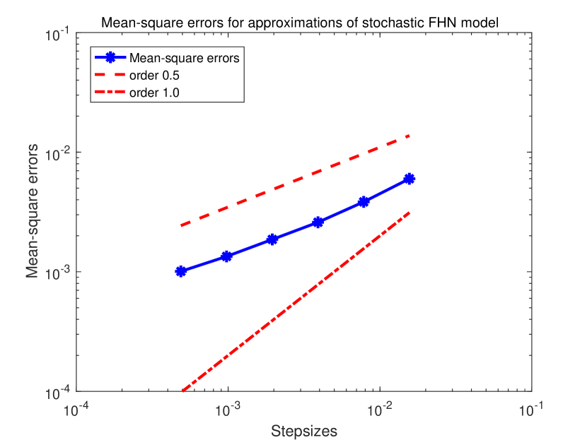
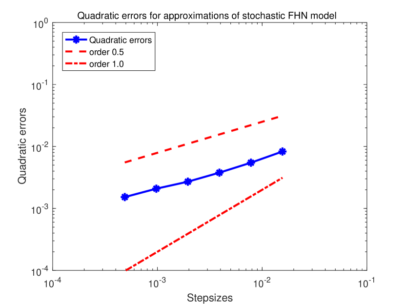
Firstly, we test the strong convergence rate of the (TMS1) by averaging over $10^{5}$ numerically generated samples. Besides, the ”exact” solutions are identified numerically using a fine stepsize $h_{\text{exact}}=2^{-15}$. We depict the mean-square approximation errors $\|X_{T}-Y_{T/h}\|_{L^{2}(\Omega,\mathbb{R}^{2})}$ and quadratic approximation errors $\|X_{T}-Y_{T/h}\|_{L^{4}(\Omega,\mathbb{R}^{2})}$ against six different stepsizes $h=2^{-6},2^{-7},\dots,2^{-11}$ on a log-log scale. Also included are two reference lines with slopes of $0.5$ and $1$, which reflect order $0.5$ and order $1$, respectively. From Figure 1 one can easily observe that both approximation errors decrease at a slope close to $0.5$ when stepsizes shrink, coinciding with the theoretical findings obtained in Theorem 4.6.

Refer to caption
Refer to caption
Figure 1: Strong convergence rates of the Tamed Milstein scheme (TMS1) for the generalized stochastic FHN model (6.1) in mean-squred sense (Left) and in quadratic sense (Right)

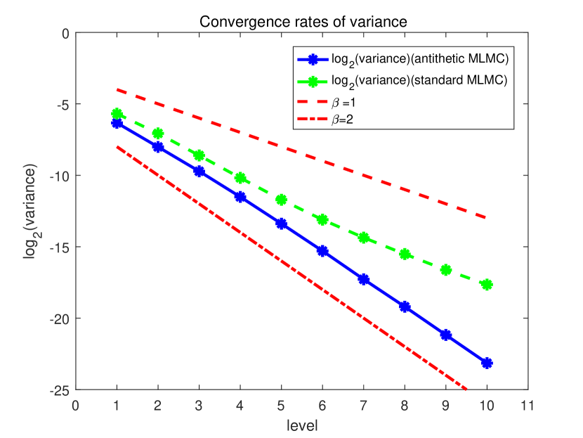
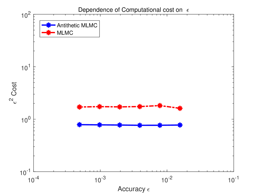
Let us proceed by following Theorem 2.1 to investigate the convergence behavior of variance as a function of the level of approximation and the computational cost for a smooth payoff function $P=2X_{1}(T)+\sin(X_{2}(T))$. On the left side of Figure 2, we employ $10^{5}$ samples to show the variance of the multilevel estimators at 10 different levels. Reference lines with slopes of $-1$ and $-2$ are given, which confirms $\beta=1$ with the standard MLMC and $\beta=2$ with the antithetic MLMC, respectively. On the right side of Figure 2, the solid line represents the dependence of complexity as function of the desired accuracy $\epsilon$ with the antithetic MLMC technique while the dotted line represents this by the standard MLMC. We see that the complexity of antithetic MLMC is proportional to $\epsilon^{2}$ and is much lower than standard MLMC.

Refer to caption
Refer to caption
Figure 2: Convergence rates of variance (Left) and computational cost (Right) for a smooth payoff function $P=2X_{1}(T)+\sin(X_{2}(T))$

References

  • [1] W.-J. Beyn, E.Β Isaak, and R.Β Kruse. Stochastic C-stability and B-consistency of explicit and implicit Euler-type schemes. Journal of Scientific Computing, 67(3):955–987, 2016.
  • [2] W.-J. Beyn, E.Β Isaak, and R.Β Kruse. Stochastic C-stability and B-consistency of explicit and implicit Milstein-type schemes. Journal of Scientific Computing, 70(3):1042–1077, 2017.
  • [3] J.Β M. Clark and R.Β Cameron. The maximum rate of convergence of discrete approximations for stochastic differential equations. In Stochastic differential systems filtering and control, pages 162–171. Springer, 1980.
  • [4] D.Β Duffie and P.Β Glynn. Efficient Monte Carlo simulation of security prices. The Annals of Applied Probability, pages 897–905, 1995.
  • [5] M.Β Giles. Improved multilevel Monte Carlo convergence using the Milstein scheme. In Monte Carlo and Quasi-Monte Carlo Methods 2006, pages 343–358. Springer, 2008.
  • [6] M.Β B. Giles. Multilevel monte carlo path simulation. Operations research, 56(3):607–617, 2008.
  • [7] M.Β B. Giles and L.Β Szpruch. Antithetic multilevel Monte Carlo estimation for multi-dimensional SDEs without LΓ©vy area simulation. The Annals of Applied Probability, 24(4):1585–1620, 2014.
  • [8] D.Β J. Higham. An introduction to multilevel monte carlo for option valuation. International Journal of Computer Mathematics, 92(12):2347–2360, 2015.
  • [9] D.Β J. Higham, X.Β Mao, and A.Β M. Stuart. Strong convergence of Euler-type methods for nonlinear stochastic differential equations. SIAM Journal on Numerical Analysis, 40(3):1041–1063, 2002.
  • [10] Y.Β Hu. Semi-implicit Euler-Maruyama scheme for stiff stochastic equations. in Stochastic Analysis and Related Topics V: The Silvri Workshop, Progr. Probab., 38:183–202, 1996.
  • [11] M.Β Hutzenthaler and A.Β Jentzen. Convergence of the stochastic Euler scheme for locally Lipschitz coefficients. Foundations of Computational Mathematics, 11(6):657–706, 2011.
  • [12] M.Β Hutzenthaler, A.Β Jentzen, and P.Β E. Kloeden. Strong convergence of an explicit numerical method for SDEs with nonglobally Lipschitz continuous coefficients. The Annals of Applied Probability, 22(4):1611–1641, 2010.
  • [13] M.Β Hutzenthaler, A.Β Jentzen, and P.Β E. Kloeden. Strong and weak divergence in finite time of Euler’s method for stochastic differential equations with non-globally Lipschitz continuous coefficients. Proceedings of the Royal Society A: Mathematical, Physical and Engineering Sciences, 467(2130):1563–1576, 2011.
  • [14] M.Β Hutzenthaler, A.Β Jentzen, and P.Β E. Kloeden. Strong convergence of an explicit numerical method for SDEs with nonglobally Lipschitz continuous coefficients. The Annals of Applied Probability, 22(4):1611–1641, 2012.
  • [15] M.Β Hutzenthaler, A.Β Jentzen, and P.Β E. Kloeden. Divergence of the multilevel Monte Carlo Euler method for nonlinear stochastic differential equations. The Annals of Applied Probability, 23(5):1913–1966, 2013.
  • [16] A.Β Jentzen. Stochastic partial differential equations: analysis and numerical approximations. Lecture notes, ETH Zurich, summer semester, 2016.
  • [17] A.Β Kebaier. Statistical Romberg extrapolation: a new variance reduction method and applications to option pricing. The Annals of Applied Probability, 15(4):2681–2705, 2005.
  • [18] C.Β Kelly and G.Β J. Lord. Adaptive Euler methods for stochastic systems with non-globally Lipschitz coefficients. Numerical Algorithms, 89:721–747, 2022.
  • [19] C.Β Kumar and S.Β Sabanis. On Milstein approximations with varying coefficients: the case of super-linear diffusion coefficients. BIT Numerical Mathematics, 59(4):929–968, 2019.
  • [20] X.Β Li, X.Β Mao, and G.Β Yin. Explicit numerical approximations for stochastic differential equations in finite and infinite horizons: truncation methods, convergence in p th moment and stability. IMA Journal of Numerical Analysis, 39(2):847–892, 2019.
  • [21] X.Β Mao. Stochastic differential equations and applications. Elsevier, 2007.
  • [22] A.Β Neuenkirch and L.Β Szpruch. First order strong approximations of scalar SDEs defined in a domain. Numerische Mathematik, 128(1):103–136, 2014.
  • [23] S.Β Sabanis. Euler approximations with varying coefficients: the case of superlinearly growing diffusion coefficients. The Annals of Applied Probability, 26(4):2083–2105, 2016.
  • [24] X.Β Wang. Strong convergence rates of the linear implicit Euler method for the finite element discretization of SPDEs with additive noise. IMA Journal of Numerical Analysis, 37(2):965–984, 2017.
  • [25] X.Β Wang. Mean-square convergence rates of implicit Milstein type methods for SDEs with non-Lipschitz coefficients. Advances in Computational Mathematics, DOI:10.1007/s10444-023-10034-2, 2023.
  • [26] X.Β Wang and S.Β Gan. The tamed Milstein method for commutative stochastic differential equations with non-globally Lipschitz continuous coefficients. Journal of Difference Equations and Applications, 19(3):466–490, 2013.
  • [27] X.Β Wang, J.Β Wu, and B.Β Dong. Mean-square convergence rates of stochastic theta methods for SDEs under a coupled monotonicity condition. BIT Numerical Mathematics, 60(3):759–790, 2020.
  • [28] H.Β Yang and X.Β Li. Explicit approximations for nonlinear switching diffusion systems in finite and infinite horizons. Journal of Differential Equations, 265(7):2921–2967, 2018.

Appendix A Proof of Theorem 4.1

Proof of Theorem 4.1.

Baesd on (3.11), we can deduce that, for any $n\in\{0,1,\dots,N-1\}$, $N\in\mathbb{N}$,

$\displaystyle\|Y_{n+1}\|^{2}$ (A.1)
=‖𝒫​(Yn)+ΞΌh​(𝒫​(Yn))​h+Οƒh​(𝒫​(Yn))​Δ​Wn+βˆ‘j1,j2=1m(β„’j1​σj2)h​(𝒫​(Yn))​Πj1,j2tn,tn+1β€–2absentsuperscriptnorm𝒫subscriptπ‘Œπ‘›subscriptπœ‡β„Žπ’«subscriptπ‘Œπ‘›β„ŽsubscriptπœŽβ„Žπ’«subscriptπ‘Œπ‘›Ξ”subscriptπ‘Šπ‘›superscriptsubscriptsubscript𝑗1subscript𝑗21π‘šsubscriptsuperscriptβ„’subscript𝑗1subscript𝜎subscript𝑗2β„Žπ’«subscriptπ‘Œπ‘›superscriptsubscriptΞ subscript𝑗1subscript𝑗2subscript𝑑𝑛subscript𝑑𝑛12\displaystyle=\Big{\|}\mathscr{P}(Y_{n})+\mu_{h}\left(\mathscr{P}(Y_{n})\right)h+\sigma_{h}\left(\mathscr{P}(Y_{n})\right)\Delta W_{n}+\sum_{j_{1},j_{2}=1}^{m}\left(\mathcal{L}^{j_{1}}\sigma_{j_{2}}\right)_{h}\left(\mathscr{P}(Y_{n})\right)\Pi_{j_{1},j_{2}}^{t_{n},t_{n+1}}\Big{\|}^{2}
=‖𝒫​(Yn)β€–2+h2​‖μh​(𝒫​(Yn))β€–2+β€–Οƒh​(𝒫​(Yn))​Δ​Wnβ€–2+β€–βˆ‘j1,j2=1m(β„’j1​σj2)h​(𝒫​(Yn))​Πj1,j2tn,tn+1β€–2absentsuperscriptnorm𝒫subscriptπ‘Œπ‘›2superscriptβ„Ž2superscriptnormsubscriptπœ‡β„Žπ’«subscriptπ‘Œπ‘›2superscriptnormsubscriptπœŽβ„Žπ’«subscriptπ‘Œπ‘›Ξ”subscriptπ‘Šπ‘›2superscriptnormsuperscriptsubscriptsubscript𝑗1subscript𝑗21π‘šsubscriptsuperscriptβ„’subscript𝑗1subscript𝜎subscript𝑗2β„Žπ’«subscriptπ‘Œπ‘›superscriptsubscriptΞ subscript𝑗1subscript𝑗2subscript𝑑𝑛subscript𝑑𝑛12\displaystyle=\|\mathscr{P}(Y_{n})\|^{2}+h^{2}\|\mu_{h}\left(\mathscr{P}(Y_{n})\right)\|^{2}+\|\sigma_{h}\left(\mathscr{P}(Y_{n})\right)\Delta W_{n}\|^{2}+\Big{\|}\sum_{j_{1},j_{2}=1}^{m}\left(\mathcal{L}^{j_{1}}\sigma_{j_{2}}\right)_{h}\left(\mathscr{P}(Y_{n})\right)\Pi_{j_{1},j_{2}}^{t_{n},t_{n+1}}\Big{\|}^{2}
+2​hβ€‹βŸ¨π’«β€‹(Yn),ΞΌh​(𝒫​(Yn))⟩+2β€‹βŸ¨π’«β€‹(Yn),Οƒh​(𝒫​(Yn))​Δ​Wn⟩+2β€‹βˆ‘j1,j2=1mβŸ¨π’«β€‹(Yn),(β„’j1​σj2)h​(𝒫​(Yn))​Πj1,j2tn,tn+1⟩2β„Žπ’«subscriptπ‘Œπ‘›subscriptπœ‡β„Žπ’«subscriptπ‘Œπ‘›2𝒫subscriptπ‘Œπ‘›subscriptπœŽβ„Žπ’«subscriptπ‘Œπ‘›Ξ”subscriptπ‘Šπ‘›2superscriptsubscriptsubscript𝑗1subscript𝑗21π‘šπ’«subscriptπ‘Œπ‘›subscriptsuperscriptβ„’subscript𝑗1subscript𝜎subscript𝑗2β„Žπ’«subscriptπ‘Œπ‘›superscriptsubscriptΞ subscript𝑗1subscript𝑗2subscript𝑑𝑛subscript𝑑𝑛1\displaystyle\ +2h\left\langle\mathscr{P}(Y_{n}),\mu_{h}\left(\mathscr{P}(Y_{n})\right)\right\rangle+2\left\langle\mathscr{P}(Y_{n}),\sigma_{h}\left(\mathscr{P}(Y_{n})\right)\Delta W_{n}\right\rangle+2\sum_{j_{1},j_{2}=1}^{m}\left\langle\mathscr{P}(Y_{n}),\left(\mathcal{L}^{j_{1}}\sigma_{j_{2}}\right)_{h}\left(\mathscr{P}(Y_{n})\right)\Pi_{j_{1},j_{2}}^{t_{n},t_{n+1}}\right\rangle
+2​hβ€‹βŸ¨ΞΌh​(𝒫​(Yn)),Οƒh​(𝒫​(Yn))​Δ​Wn⟩+2β€‹βˆ‘j1,j2=1mβŸ¨Οƒh​(𝒫​(Yn))​Δ​Wn,(β„’j1​σj2)h​(𝒫​(Yn))​Πj1,j2tn,tn+1⟩2β„Žsubscriptπœ‡β„Žπ’«subscriptπ‘Œπ‘›subscriptπœŽβ„Žπ’«subscriptπ‘Œπ‘›Ξ”subscriptπ‘Šπ‘›2superscriptsubscriptsubscript𝑗1subscript𝑗21π‘šsubscriptπœŽβ„Žπ’«subscriptπ‘Œπ‘›Ξ”subscriptπ‘Šπ‘›subscriptsuperscriptβ„’subscript𝑗1subscript𝜎subscript𝑗2β„Žπ’«subscriptπ‘Œπ‘›superscriptsubscriptΞ subscript𝑗1subscript𝑗2subscript𝑑𝑛subscript𝑑𝑛1\displaystyle\ +2h\left\langle\mu_{h}\left(\mathscr{P}(Y_{n})\right),\sigma_{h}\left(\mathscr{P}(Y_{n})\right)\Delta W_{n}\right\rangle+2\sum_{j_{1},j_{2}=1}^{m}\left\langle\sigma_{h}\left(\mathscr{P}(Y_{n})\right)\Delta W_{n},\left(\mathcal{L}^{j_{1}}\sigma_{j_{2}}\right)_{h}\left(\mathscr{P}(Y_{n})\right)\Pi_{j_{1},j_{2}}^{t_{n},t_{n+1}}\right\rangle
+2​hβ€‹βˆ‘j1,j2=1m⟨μh​(𝒫​(Yn)),(β„’j1​σj2)h​(𝒫​(Yn))​Πj1,j2tn,tn+1⟩.2β„Žsuperscriptsubscriptsubscript𝑗1subscript𝑗21π‘šsubscriptπœ‡β„Žπ’«subscriptπ‘Œπ‘›subscriptsuperscriptβ„’subscript𝑗1subscript𝜎subscript𝑗2β„Žπ’«subscriptπ‘Œπ‘›superscriptsubscriptΞ subscript𝑗1subscript𝑗2subscript𝑑𝑛subscript𝑑𝑛1\displaystyle\ +2h\sum_{j_{1},j_{2}=1}^{m}\left\langle\mu_{h}\left(\mathscr{P}(Y_{n})\right),\left(\mathcal{L}^{j_{1}}\sigma_{j_{2}}\right)_{h}\left(\mathscr{P}(Y_{n})\right)\Pi_{j_{1},j_{2}}^{t_{n},t_{n+1}}\right\rangle.

Using the Young inequality $2ab\leq\frac{\epsilon_{1}}{2}a^{2}+\frac{2}{\epsilon_{1}}b^{2}$, $\epsilon_{1}\in(0,2p_{0}-2p]$ and Assumption 3.3 implies that, for $j_{1},j_{2}\in\{1,\dots,m\}$,

$\displaystyle 2h\left\langle\mu_{h}\left(\mathscr{P}(Y_{n})\right),\sigma_{h}\left(\mathscr{P}(Y_{n})\right)\Delta W_{n}\right\rangle$ $\displaystyle\leq\tfrac{2}{\epsilon_{1}}h^{2}\|\mu_{h}\left(\mathscr{P}(Y_{n})\right)\|^{2}+\tfrac{\epsilon_{1}}{2}\|\sigma_{h}\left(\mathscr{P}(Y_{n})\right)\Delta W_{n}\|^{2},$ (A.2)
$\displaystyle\leq C_{\epsilon_{1}}h(1+\|\mathscr{P}(Y_{n})\|)^{2}+\tfrac{\epsilon_{1}}{2}\|\sigma_{h}\left(\mathscr{P}(Y_{n})\right)\Delta W_{n}\|^{2},$
2β€‹βŸ¨Οƒh​(𝒫​(Yn))​Δ​Wn,(β„’j1​σj2)h​(𝒫​(Yn))​Πj1,j2tn,tn+1⟩2subscriptπœŽβ„Žπ’«subscriptπ‘Œπ‘›Ξ”subscriptπ‘Šπ‘›subscriptsuperscriptβ„’subscript𝑗1subscript𝜎subscript𝑗2β„Žπ’«subscriptπ‘Œπ‘›superscriptsubscriptΞ subscript𝑗1subscript𝑗2subscript𝑑𝑛subscript𝑑𝑛1\displaystyle 2\left\langle\sigma_{h}\left(\mathscr{P}(Y_{n})\right)\Delta W_{n},\left(\mathcal{L}^{j_{1}}\sigma_{j_{2}}\right)_{h}\left(\mathscr{P}(Y_{n})\right)\Pi_{j_{1},j_{2}}^{t_{n},t_{n+1}}\right\rangle ≀ϡ12​‖σh​(𝒫​(Yn))​Δ​Wnβ€–2+2Ο΅1​‖(β„’j1​σj2)h​(𝒫​(Yn))​Πj1,j2tn,tn+1β€–2absentsubscriptitalic-Ο΅12superscriptnormsubscriptπœŽβ„Žπ’«subscriptπ‘Œπ‘›Ξ”subscriptπ‘Šπ‘›22subscriptitalic-Ο΅1superscriptnormsubscriptsuperscriptβ„’subscript𝑗1subscript𝜎subscript𝑗2β„Žπ’«subscriptπ‘Œπ‘›superscriptsubscriptΞ subscript𝑗1subscript𝑗2subscript𝑑𝑛subscript𝑑𝑛12\displaystyle\leq\tfrac{\epsilon_{1}}{2}\left\|\sigma_{h}\left(\mathscr{P}(Y_{n})\right)\Delta W_{n}\right\|^{2}+\tfrac{2}{\epsilon_{1}}\Big{\|}\left(\mathcal{L}^{j_{1}}\sigma_{j_{2}}\right)_{h}\left(\mathscr{P}(Y_{n})\right)\Pi_{j_{1},j_{2}}^{t_{n},t_{n+1}}\Big{\|}^{2}
≀ϡ12​‖σh​(𝒫​(Yn))​Δ​Wnβ€–2+CΟ΅1h​(1+‖𝒫​(Yn)β€–)2​|Ξ j1,j2tn,tn+1|2,absentsubscriptitalic-Ο΅12superscriptnormsubscriptπœŽβ„Žπ’«subscriptπ‘Œπ‘›Ξ”subscriptπ‘Šπ‘›2subscript𝐢subscriptitalic-Ο΅1β„Žsuperscript1norm𝒫subscriptπ‘Œπ‘›2superscriptsuperscriptsubscriptΞ subscript𝑗1subscript𝑗2subscript𝑑𝑛subscript𝑑𝑛12\displaystyle\leq\tfrac{\epsilon_{1}}{2}\left\|\sigma_{h}\left(\mathscr{P}(Y_{n})\right)\Delta W_{n}\right\|^{2}+\tfrac{C_{\epsilon_{1}}}{h}(1+\|\mathscr{P}(Y_{n})\|)^{2}\left|\Pi_{j_{1},j_{2}}^{t_{n},t_{n+1}}\right|^{2},
2​hβ€‹βŸ¨ΞΌh​(𝒫​(Yn)),(β„’j1​σj2)h​(𝒫​(Yn))​Πj1,j2tn,tn+1⟩2β„Žsubscriptπœ‡β„Žπ’«subscriptπ‘Œπ‘›subscriptsuperscriptβ„’subscript𝑗1subscript𝜎subscript𝑗2β„Žπ’«subscriptπ‘Œπ‘›superscriptsubscriptΞ subscript𝑗1subscript𝑗2subscript𝑑𝑛subscript𝑑𝑛1\displaystyle 2h\left\langle\mu_{h}\left(\mathscr{P}(Y_{n})\right),\left(\mathcal{L}^{j_{1}}\sigma_{j_{2}}\right)_{h}\left(\mathscr{P}(Y_{n})\right)\Pi_{j_{1},j_{2}}^{t_{n},t_{n+1}}\right\rangle ≀h2​‖μh​(𝒫​(Yn))β€–2+β€–(β„’j1​σj2)h​(𝒫​(Yn))​Πj1,j2tn,tn+1β€–2absentsuperscriptβ„Ž2superscriptnormsubscriptπœ‡β„Žπ’«subscriptπ‘Œπ‘›2superscriptnormsubscriptsuperscriptβ„’subscript𝑗1subscript𝜎subscript𝑗2β„Žπ’«subscriptπ‘Œπ‘›superscriptsubscriptΞ subscript𝑗1subscript𝑗2subscript𝑑𝑛subscript𝑑𝑛12\displaystyle\leq h^{2}\|\mu_{h}\left(\mathscr{P}(Y_{n})\right)\|^{2}+\Big{\|}\left(\mathcal{L}^{j_{1}}\sigma_{j_{2}}\right)_{h}\left(\mathscr{P}(Y_{n})\right)\Pi_{j_{1},j_{2}}^{t_{n},t_{n+1}}\Big{\|}^{2}
≀C​h​(1+‖𝒫​(Yn)β€–)2+CΟ΅1h​(1+‖𝒫​(Yn)β€–)2​|Ξ j1,j2tn,tn+1|2.absentπΆβ„Žsuperscript1norm𝒫subscriptπ‘Œπ‘›2subscript𝐢subscriptitalic-Ο΅1β„Žsuperscript1norm𝒫subscriptπ‘Œπ‘›2superscriptsuperscriptsubscriptΞ subscript𝑗1subscript𝑗2subscript𝑑𝑛subscript𝑑𝑛12\displaystyle\leq Ch(1+\|\mathscr{P}(Y_{n})\|)^{2}+\tfrac{C_{\epsilon_{1}}}{h}(1+\|\mathscr{P}(Y_{n})\|)^{2}\left|\Pi_{j_{1},j_{2}}^{t_{n},t_{n+1}}\right|^{2}.

Therefore, one can derive that

$\displaystyle 1+\|Y_{n+1}\|^{2}\leq(1+\|\mathscr{P}(Y_{n})\|^{2})(1+\xi_{n+1}),$ (A.3)

where

$\displaystyle\xi_{n+1}$ (A.4)
:=CΟ΅1​h​(1+‖𝒫​(Yn)β€–)21+‖𝒫​(Yn)β€–2βŸβ‰€CΟ΅1​h+(1+Ο΅1)​‖σh​(𝒫​(Yn))​Δ​Wnβ€–21+‖𝒫​(Yn)β€–2⏟=⁣:I1+CΟ΅1h​(1+‖𝒫​(Yn)β€–)2β€‹βˆ‘j1,j2=1m|Ξ j1,j2tn,tn+1|21+‖𝒫​(Yn)β€–2⏟=⁣:I2+2​hβ€‹βŸ¨π’«β€‹(Yn),ΞΌh​(𝒫​(Yn))⟩1+‖𝒫​(Yn)β€–2⏟=⁣:I3assignabsentsubscript⏟subscript𝐢subscriptitalic-Ο΅1β„Žsuperscript1norm𝒫subscriptπ‘Œπ‘›21superscriptnorm𝒫subscriptπ‘Œπ‘›2absentsubscript𝐢subscriptitalic-Ο΅1β„Žsubscript⏟1subscriptitalic-Ο΅1superscriptnormsubscriptπœŽβ„Žπ’«subscriptπ‘Œπ‘›Ξ”subscriptπ‘Šπ‘›21superscriptnorm𝒫subscriptπ‘Œπ‘›2:absentsubscript𝐼1subscript⏟subscript𝐢subscriptitalic-Ο΅1β„Žsuperscript1norm𝒫subscriptπ‘Œπ‘›2superscriptsubscriptsubscript𝑗1subscript𝑗21π‘šsuperscriptsuperscriptsubscriptΞ subscript𝑗1subscript𝑗2subscript𝑑𝑛subscript𝑑𝑛121superscriptnorm𝒫subscriptπ‘Œπ‘›2:absentsubscript𝐼2subscript⏟2β„Žπ’«subscriptπ‘Œπ‘›subscriptπœ‡β„Žπ’«subscriptπ‘Œπ‘›1superscriptnorm𝒫subscriptπ‘Œπ‘›2:absentsubscript𝐼3\displaystyle:=\underbrace{\tfrac{C_{\epsilon_{1}}h(1+\|\mathscr{P}(Y_{n})\|)^{2}}{1+\|\mathscr{P}(Y_{n})\|^{2}}}_{\leq C_{\epsilon_{1}}h}+\underbrace{\tfrac{(1+\epsilon_{1})\|\sigma_{h}\left(\mathscr{P}(Y_{n})\right)\Delta W_{n}\|^{2}}{1+\|\mathscr{P}(Y_{n})\|^{2}}}_{=:I_{1}}+\underbrace{\tfrac{\frac{C_{\epsilon_{1}}}{h}(1+\|\mathscr{P}(Y_{n})\|)^{2}\sum_{j_{1},j_{2}=1}^{m}\left|\Pi_{j_{1},j_{2}}^{t_{n},t_{n+1}}\right|^{2}}{1+\|\mathscr{P}(Y_{n})\|^{2}}}_{=:I_{2}}+\underbrace{\tfrac{2h\left\langle\mathscr{P}(Y_{n}),\mu_{h}\left(\mathscr{P}(Y_{n})\right)\right\rangle}{1+\|\mathscr{P}(Y_{n})\|^{2}}}_{=:I_{3}}
+2β€‹βˆ‘j1,j2=1mβŸ¨π’«β€‹(Yn),(β„’j1​σj2)h​(𝒫​(Yn))​Πj1,j2tn,tn+1⟩1+‖𝒫​(Yn)β€–2⏟=⁣:I4+2β€‹βŸ¨π’«β€‹(Yn),Οƒh​(𝒫​(Yn))​Δ​Wn⟩1+‖𝒫​(Yn)β€–2⏟=⁣:I5.subscript⏟2superscriptsubscriptsubscript𝑗1subscript𝑗21π‘šπ’«subscriptπ‘Œπ‘›subscriptsuperscriptβ„’subscript𝑗1subscript𝜎subscript𝑗2β„Žπ’«subscriptπ‘Œπ‘›superscriptsubscriptΞ subscript𝑗1subscript𝑗2subscript𝑑𝑛subscript𝑑𝑛11superscriptnorm𝒫subscriptπ‘Œπ‘›2:absentsubscript𝐼4subscript⏟2𝒫subscriptπ‘Œπ‘›subscriptπœŽβ„Žπ’«subscriptπ‘Œπ‘›Ξ”subscriptπ‘Šπ‘›1superscriptnorm𝒫subscriptπ‘Œπ‘›2:absentsubscript𝐼5\displaystyle\ +\underbrace{\tfrac{2\sum_{j_{1},j_{2}=1}^{m}\left\langle\mathscr{P}(Y_{n}),\left(\mathcal{L}^{j_{1}}\sigma_{j_{2}}\right)_{h}\left(\mathscr{P}(Y_{n})\right)\Pi_{j_{1},j_{2}}^{t_{n},t_{n+1}}\right\rangle}{1+\|\mathscr{P}(Y_{n})\|^{2}}}_{=:I_{4}}+\underbrace{\tfrac{2\langle\mathscr{P}(Y_{n}),\sigma_{h}\left(\mathscr{P}(Y_{n})\right)\Delta W_{n}\rangle}{1+\|\mathscr{P}(Y_{n})\|^{2}}}_{=:I_{5}}.

Taking the $p$-th power, $p\in[1,p_{0})$, and the conditional mathematical expectation with respect to $\mathcal{F}_{t_{n}}$ on both sides of (A.3) yields

$\displaystyle\mathbb{E}\left[\left(1+\|Y_{n+1}\|^{2}\right)^{p}\big{|}\mathcal{F}_{t_{n}}\right]\leq(1+\|\mathscr{P}(Y_{n})\|^{2})^{p}\mathbb{E}\left[\left(1+\xi_{n+1}\right)^{p}\big{|}\mathcal{F}_{t_{n}}\right].$ (A.5)

According to Lemma 3.3 in [28], given any $p\in(i,i+1]$, $i\in\mathbb{N}$, the following estimate

$\displaystyle\mathbb{E}\left[\left(1+\xi_{n+1}\right)^{p}\big{|}\mathcal{F}_{t_{n}}\right]\leq 1+p\mathbb{E}\left[\xi_{n+1}\big{|}\mathcal{F}_{t_{n}}\right]+\tfrac{p(p-1)}{2}\mathbb{E}\left[\xi_{n+1}^{2}\big{|}\mathcal{F}_{t_{n}}\right]+\mathbb{E}\left[\xi_{n+1}^{3}l_{i}(\xi_{n+1})\big{|}\mathcal{F}_{t_{n}}\right]$ (A.6)

holds true for any $\xi_{n+1}>-1$, where $l_{i}(\xi)$ is represented as a polynomial of order $i$ with respect to $\xi$ whose coefficients rely only on $p$. We thus have to estimate only the last three terms in (A.6).

Step I: estimate of $\mathbb{E}\left[\xi_{n+1}|\mathcal{F}_{t_{n}}\right]$

Since $\Delta W_{n}$ and Ξ j1,j2tn,tn+1superscriptsubscriptΞ subscript𝑗1subscript𝑗2subscript𝑑𝑛subscript𝑑𝑛1\Pi_{j_{1},j_{2}}^{t_{n},t_{n+1}} are independent of $\mathcal{F}_{t_{n}}$, we have

𝔼​[Δ​Wj,n|β„±tn]=𝔼​[Ξ j1,j2tn,tn+1|β„±tn]=0,𝔼​[|Δ​Wj,n|2|β„±tn]=h,βˆ€nβˆˆβ„•,j∈{1,…,m}formulae-sequence𝔼delimited-[]conditionalΞ”subscriptπ‘Šπ‘—π‘›subscriptβ„±subscript𝑑𝑛𝔼delimited-[]conditionalsuperscriptsubscriptΞ subscript𝑗1subscript𝑗2subscript𝑑𝑛subscript𝑑𝑛1subscriptβ„±subscript𝑑𝑛0formulae-sequence𝔼delimited-[]conditionalsuperscriptΞ”subscriptπ‘Šπ‘—π‘›2subscriptβ„±subscriptπ‘‘π‘›β„Žformulae-sequencefor-all𝑛ℕ𝑗1β€¦π‘š\displaystyle\mathbb{E}\left[\Delta W_{j,n}\big{|}\mathcal{F}_{t_{n}}\right]=\mathbb{E}\left[\Pi_{j_{1},j_{2}}^{t_{n},t_{n+1}}\big{|}\mathcal{F}_{t_{n}}\right]=0,\quad\mathbb{E}\left[|\Delta W_{j,n}|^{2}\big{|}\mathcal{F}_{t_{n}}\right]=h,\quad\forall n\in\mathbb{N},\ j\in\{1,\ldots,m\} (A.7)

and thus for any $p\in[1,p_{0})$,

𝔼​[|Δ​Wj,n|p|β„±tn]≀C​hp/2,𝔼​[|Ξ j1,j2tn,tn+1|p|β„±tn]≀C​hp,βˆ€nβˆˆβ„•,j,j1,j2∈{1,…,m}.formulae-sequence𝔼delimited-[]conditionalsuperscriptΞ”subscriptπ‘Šπ‘—π‘›π‘subscriptβ„±subscript𝑑𝑛𝐢superscriptβ„Žπ‘2formulae-sequence𝔼delimited-[]conditionalsuperscriptsuperscriptsubscriptΞ subscript𝑗1subscript𝑗2subscript𝑑𝑛subscript𝑑𝑛1𝑝subscriptβ„±subscript𝑑𝑛𝐢superscriptβ„Žπ‘formulae-sequencefor-all𝑛ℕ𝑗subscript𝑗1subscript𝑗21β€¦π‘š\displaystyle\mathbb{E}\left[\left|\Delta W_{j,n}\right|^{p}\big{|}\mathcal{F}_{t_{n}}\right]\leq Ch^{p/2},\quad\mathbb{E}\left[\big{|}\Pi_{j_{1},j_{2}}^{t_{n},t_{n+1}}\big{|}^{p}\big{|}\mathcal{F}_{t_{n}}\right]\leq Ch^{p},\quad\forall n\in\mathbb{N},\ j,j_{1},j_{2}\in\{1,\ldots,m\}. (A.8)

Hence, we get

$$\mathbb{E}\left[I_{4}\big{|}\mathcal{F}_{t_{n}}\right]=\mathbb{E}\left[I_{5}\big{|}\mathcal{F}_{t_{n}}\right]=0.$$ (A.9)

Furthermore, due to (A.7)-(A.9), one can easily observe that

$\displaystyle\mathbb{E}\left[\xi_{n+1}\big{|}\mathcal{F}_{t_{n}}\right]$ $\displaystyle\leq C_{\epsilon_{1}}h+\tfrac{2h\langle\mathscr{P}(Y_{n}),\mu_{h}\left(\mathscr{P}(Y_{n})\right)\rangle+(1+\epsilon_{1})h\|\sigma_{h}\left(\mathscr{P}(Y_{n})\right)\|^{2}}{1+\|\mathscr{P}(Y_{n})\|^{2}}.$ (A.10)

Step II: estimate of $\mathbb{E}\left[\xi^{2}|\mathcal{F}_{t_{n}}\right]$

Before proceeding further, we introduce a series of useful estimates. By virtue of (A.8), (3.25) and the fact that $\Delta W_{n}$ is independent from $\mathcal{F}_{t_{n}}$, one can infer that, for $k\in\mathbb{N}$,

$\displaystyle\mathbb{E}\left[|I_{1}|^{k}\big{|}\mathcal{F}_{t_{n}}\right]$ $\displaystyle=\tfrac{(1+\epsilon_{1})^{k}\mathbb{E}\left[\|\sigma_{h}\left(\mathscr{P}(Y_{n})\right)\Delta W_{n}\|^{2k}\big{|}\mathcal{F}_{t_{n}}\right]}{(1+\|\mathscr{P}(Y_{n})\|^{2})^{k}}\leq\tfrac{Ch^{\frac{k}{2}}\left(1+\|\mathscr{P}(Y_{n})\|^{2}\right)^{k}}{(1+\|\mathscr{P}(Y_{n})\|^{2})^{k}}\leq Ch^{k/2}.$ (A.11)

Owing to (A.8), we then acquire

$\displaystyle\mathbb{E}\left[|I_{2}|^{k}\big{|}\mathcal{F}_{t_{n}}\right]\leq C_{\epsilon_{1}}h^{k}.$ (A.12)

By Assumption 3.3 and the Cauchy-Schwarz inequality, we also obtain that,

$\displaystyle\mathbb{E}\left[|I_{3}|^{k}\big{|}\mathcal{F}_{t_{n}}\right]=\tfrac{2^{k}h^{k}\left|\langle\mathscr{P}(Y_{n}),\mu_{h}\left(\mathscr{P}(Y_{n})\right)\rangle\right|^{k}}{(1+\|\mathscr{P}(Y_{n})\|^{2})^{k}}\leq\tfrac{Ch^{k}\|\mathscr{P}(Y_{n})\|^{k}\|\mu_{h}\left(\mathscr{P}(Y_{n})\right)\|^{k}}{(1+\|\mathscr{P}(Y_{n})\|^{2})^{k}}\leq Ch^{k/2}.$ (A.13)

Analogous to (A.13), using the Cauchy-Schwarz inequality and (A.8) implies that

$\displaystyle\mathbb{E}\left[|I_{4}|^{k}\big{|}\mathcal{F}_{t_{n}}\right]$ $\displaystyle\leq\tfrac{2^{k}h^{k}\sum_{j_{1},j_{2}=1}^{m}\left|\left\langle\mathscr{P}(Y_{n}),\left(\mathcal{L}^{j_{1}}\sigma_{j_{2}}\right)_{h}\left(\mathscr{P}(Y_{n})\right)\right\rangle\right|^{k}}{(1+\|\mathscr{P}(Y_{n})\|^{2})^{k}}\leq\tfrac{Ch^{k}\sum_{j_{1},j_{2}=1}^{m}\|\mathscr{P}(Y_{n})\|^{k}\big{\|}\left(\mathcal{L}^{j_{1}}\sigma_{j_{2}}\right)_{h}\left(\mathscr{P}(Y_{n})\right)\big{\|}^{k}}{(1+\|\mathscr{P}(Y_{n})\|^{2})^{k}}\leq Ch^{k/2}.$ (A.14)

Also, due to (3.25),(A.8) and the Cauchy-Schwarz inequality, for $k\geq 4$, one observes

$\displaystyle\mathbb{E}\left[|I_{5}|^{k}\big{|}\mathcal{F}_{t_{n}}\right]$ $\displaystyle\leq\tfrac{2^{k}\|\mathscr{P}(Y_{n})\|^{k}\mathbb{E}\left[\|\sigma_{h}\left(\mathscr{P}(Y_{n})\right)\Delta W_{n}\|^{k}\big{|}\mathcal{F}_{t_{n}}\right]}{\left(1+\|\mathscr{P}(Y_{n})\|^{2}\right)^{k}}\leq\tfrac{Ch^{k/4}\|\mathscr{P}(Y_{n})\|^{k}\left(1+\|\mathscr{P}(Y_{n})\|^{2}\right)^{k/2}}{\left(1+\|\mathscr{P}(Y_{n})\|^{2}\right)^{k}}\leq Ch^{k/4}.$ (A.15)

When it comes to the estimate of $\mathbb{E}\left[\xi_{n+1}^{2}\big{|}\mathcal{F}_{t_{n}}\right]$, we use elementary inequalities to attain

$\displaystyle\mathbb{E}\big{[}\xi_{n+1}^{2}\big{|}\mathcal{F}_{t_{n}}\big{]}$ $\displaystyle=\mathbb{E}\Big{[}\Big{(}C_{\epsilon_{1}}h+\sum_{i=1}^{4}I_{i}+I_{5}\Big{)}^{2}\Big{|}\mathcal{F}_{t_{n}}\Big{]}$ (A.16)
$\displaystyle\leq C_{\epsilon_{1}}h+4\sum_{i=1}^{4}\mathbb{E}\left[I_{i}^{2}\big{|}\mathcal{F}_{t_{n}}\right]+\mathbb{E}\left[I_{5}^{2}\big{|}\mathcal{F}_{t_{n}}\right]+2\sum_{i=1}^{4}\mathbb{E}\left[I_{i}I_{5}\big{|}\mathcal{F}_{t_{n}}\right],$

where, by (A.7) we know

$\displaystyle\mathbb{E}\left[|I_{5}|^{2}\big{|}\mathcal{F}_{t_{n}}\right]=$ $\displaystyle\tfrac{4h\|\mathscr{P}(Y_{n})^{T}\sigma_{h}\left(\mathscr{P}(Y_{n})\right)\|^{2}}{(1+\|\mathscr{P}(Y_{n})\|^{2})^{2}}.$ (A.17)

Moreover, recalling some power properties of Brownian motions, for any $\overline{p}\in[1,p^{*})\cap\mathbb{N}$ and $j,j_{1},j_{2}\in\{1,\dots,m\}$, we obtain that

𝔼​[Δ​Wj,n​Πj1,j2tn,tn+1|β„±tn]=0,𝔼​[(Δ​Wj,n)2​pΒ―βˆ’1|β„±tn]=0,𝔼​[Δ​Wj,n​|Ξ j1,j2tn,tn+1|2|β„±tn]=0.formulae-sequence𝔼delimited-[]conditionalΞ”subscriptπ‘Šπ‘—π‘›superscriptsubscriptΞ subscript𝑗1subscript𝑗2subscript𝑑𝑛subscript𝑑𝑛1subscriptβ„±subscript𝑑𝑛0formulae-sequence𝔼delimited-[]conditionalsuperscriptΞ”subscriptπ‘Šπ‘—π‘›2¯𝑝1subscriptβ„±subscript𝑑𝑛0𝔼delimited-[]conditionalΞ”subscriptπ‘Šπ‘—π‘›superscriptsuperscriptsubscriptΞ subscript𝑗1subscript𝑗2subscript𝑑𝑛subscript𝑑𝑛12subscriptβ„±subscript𝑑𝑛0\mathbb{E}\left[\Delta W_{j,n}\ \Pi_{j_{1},j_{2}}^{t_{n},t_{n+1}}\big{|}\mathcal{F}_{t_{n}}\right]=0,\quad\mathbb{E}\left[\left(\Delta W_{j,n}\right)^{2\overline{p}-1}\big{|}\mathcal{F}_{t_{n}}\right]=0,\quad\mathbb{E}\left[\Delta W_{j,n}\ \big{|}\Pi_{j_{1},j_{2}}^{t_{n},t_{n+1}}\big{|}^{2}\Big{|}\mathcal{F}_{t_{n}}\right]=0. (A.18)

In view of (A.7), it is straightforward to see that

$\displaystyle\mathbb{E}\left[I_{1}I_{5}\big{|}\mathcal{F}_{t_{n}}\right]=\mathbb{E}\left[I_{2}I_{5}\big{|}\mathcal{F}_{t_{n}}\right]=\mathbb{E}\left[I_{3}I_{5}\big{|}\mathcal{F}_{t_{n}}\right]=\mathbb{E}\left[I_{4}I_{5}\big{|}\mathcal{F}_{t_{n}}\right]=0.$ (A.19)

Using (A.11)-(A.15), (A.17) and (A.19), we derive from (A.16) that

$\displaystyle\mathbb{E}\left[\xi_{n+1}^{2}\big{|}\mathcal{F}_{t_{n}}\right]\leq C_{\epsilon_{1}}h+\tfrac{4h\|\mathscr{P}(Y_{n})^{T}\sigma_{h}\left(\mathscr{P}(Y_{n})\right)\|^{2}}{(1+\|\mathscr{P}(Y_{n})\|^{2})^{2}}.$ (A.20)

Step III: estimate of $\mathbb{E}\left[\xi_{n+1}^{3}|\mathcal{F}_{t_{n}}\right]$

We begin with the following estimate from (A.18)

$\displaystyle\mathbb{E}\big{[}\left(I_{5}\right)^{3}\big{|}\mathcal{F}_{t_{n}}\big{]}=0.$ (A.21)

This together with (A.11)-(A.15) and the elementary inequality yields

$\displaystyle\mathbb{E}\left[\xi_{n+1}^{3}\big{|}\mathcal{F}_{t_{n}}\right]$ $\displaystyle=\mathbb{E}\left[\Big{(}C_{\epsilon_{1}}h+I_{5}+\sum_{i=1}^{4}I_{i}\Big{)}^{3}\Big{|}\mathcal{F}_{t_{n}}\right]$ (A.22)
$\displaystyle\leq C_{\epsilon_{1}}h+\mathbb{E}\left[\Big{(}I_{5}+\sum_{i=1}^{4}I_{i}\Big{)}^{3}\Big{|}\mathcal{F}_{t_{n}}\right]$
$\displaystyle\leq C_{\epsilon_{1}}h+\mathbb{E}\left[\Big{(}\sum_{i=1}^{4}I_{i}\Big{)}^{3}+3I_{5}\Big{(}\sum_{i=1}^{4}I_{i}\Big{)}^{2}+3I_{5}^{2}\Big{(}\sum_{i=1}^{4}I_{i}\Big{)}\Big{|}\mathcal{F}_{t_{n}}\right]$
$\displaystyle\leq C_{\epsilon_{1}}h+C\sum_{i=1}^{4}\Big{(}\mathbb{E}\left[|I_{i}|^{3}\big{|}\mathcal{F}_{t_{n}}\right]+\mathbb{E}\left[|I_{5}|\cdot(I_{i})^{2}\big{|}\mathcal{F}_{t_{n}}\right]+\mathbb{E}\left[|I_{i}|\cdot(I_{5})^{2}\big{|}\mathcal{F}_{t_{n}}\right]\Big{)}.$

It follows from (A.11) to (A.15) and the HΓΆlder inequality that, for $i\in\{1,2,3,4\}$,

$\displaystyle\mathbb{E}\left[|I_{5}|\cdot(I_{i})^{2}\big{|}\mathcal{F}_{t_{n}}\right]\leq Ch^{5/4}\leq Ch,\quad\mathbb{E}\left[|I_{i}|\cdot(I_{5})^{2}\big{|}\mathcal{F}_{t_{n}}\right]\leq Ch.$ (A.23)

As discussed above, we get

$$\mathbb{E}\left[\xi_{n+1}^{3}\big{|}\mathcal{F}_{t_{n}}\right]\leq C_{\epsilon_{1}}h.$$ (A.24)

Step IV: estimate of $\mathbb{E}\left[\xi_{n+1}^{k}|\mathcal{F}_{t_{n}}\right]$, $k\geq 4$

By virtue of the estimates from (A.11) to (A.15), one can achieve that

$\displaystyle\mathbb{E}\left[\xi_{n+1}^{k}\big{|}\mathcal{F}_{t_{n}}\right]\leq$ $\displaystyle C_{\epsilon_{1}}h+C\mathbb{E}\left[\Big{(}\sum_{i=1}^{5}I_{i}\Big{)}^{k}\Big{|}\mathcal{F}_{t_{n}}\right]\leq C_{\epsilon_{1}}h+C\sum_{i=1}^{5}\mathbb{E}\left[|I_{i}|^{k}\big{|}\mathcal{F}_{t_{n}}\right]\leq C_{\epsilon_{1}}h.$ (A.25)

Combining theses estimates from Step I to Step IV, along with Assumption 3.3, shows that, for any $p\in[1,p_{0})$,

$\displaystyle\mathbb{E}\left[\left(1+\|Y_{n+1}\|^{2}\right)^{p}\big{|}\mathcal{F}_{t_{n}}\right]$ (A.26)
$\displaystyle\leq\left(1+\|\mathscr{P}(Y_{n})\|^{2}\right)^{p}\left(1+C_{\epsilon_{1}}h+ph\tfrac{(1+\|\mathscr{P}(Y_{n})\|^{2})\big{(}2\langle\mathscr{P}(Y_{n}),\mu_{h}(\mathscr{P}(Y_{n}))\rangle+(1+\epsilon_{1})\|\sigma_{h}\left(\mathscr{P}(Y_{n})\right)\|^{2}\big{)}+2(p-1)\|\mathscr{P}(Y_{n})^{T}\sigma_{h}\left(\mathscr{P}(Y_{n})\right)\|^{2}}{(1+\|\mathscr{P}(Y_{n})\|^{2})^{2}}\right)$
$\displaystyle\leq\left(1+\|\mathscr{P}(Y_{n})\|^{2}\right)^{p}\left(1+C_{\epsilon_{1}}h+ph\tfrac{(1+\|\mathscr{P}(Y_{n})\|^{2})\big{(}2\langle\mathscr{P}(Y_{n}),\mu_{h}\left(\mathscr{P}(Y_{n})\right)\rangle+(2p-1+\epsilon_{1})\|\sigma_{h}\left(\mathscr{P}(Y_{n})\right)\|^{2}\big{)}}{(1+\|\mathscr{P}(Y_{n})\|^{2})^{2}}\right)$
$\displaystyle\leq\left(1+\|Y_{n}\|^{2}\right)^{p}(1+C_{\epsilon_{1}}h).$

Taking expectations on both sides and the proof is completed by iteration. ∎

Appendix B Proof of lemmas in Section 4

B.1 Proof of Lemma 4.2

Proof of Lemma 4.2.

We first show the moment estimate of the auxiliary process $\{\widetilde{Y}_{n}\}_{0\leq n\leq N}$ (4.2). It follows from the iteration that, for every $n\in\{0,1,\dots,N-1\}$,

Y~n+1=X0+∫0tn+1μ​(Xs)​ds+∫0tn+1σ​(Xs)​dWs⏟=Xtn+1+βˆ‘i=0nβˆ‘j1,j2=1m(β„’j1​σj2)h​(𝒫​(Yi))​Πj1,j2ti,ti+1⏟discrete​martingales.subscript~π‘Œπ‘›1subscript⏟subscript𝑋0superscriptsubscript0subscript𝑑𝑛1πœ‡subscript𝑋𝑠differential-d𝑠superscriptsubscript0subscript𝑑𝑛1𝜎subscript𝑋𝑠differential-dsubscriptπ‘Šπ‘ absentsubscript𝑋subscript𝑑𝑛1subscript⏟superscriptsubscript𝑖0𝑛superscriptsubscriptsubscript𝑗1subscript𝑗21π‘šsubscriptsuperscriptβ„’subscript𝑗1subscript𝜎subscript𝑗2β„Žπ’«subscriptπ‘Œπ‘–superscriptsubscriptΞ subscript𝑗1subscript𝑗2subscript𝑑𝑖subscript𝑑𝑖1discretemartingales\displaystyle\widetilde{Y}_{n+1}=\underbrace{X_{0}+\int_{0}^{t_{n+1}}\mu(X_{s})\ \mathrm{d}s+\int_{0}^{t_{n+1}}\sigma(X_{s})\ \mathrm{d}W_{s}}_{=X_{t_{n+1}}}+\underbrace{\sum_{i=0}^{n}\sum_{j_{1},j_{2}=1}^{m}\left(\mathcal{L}^{j_{1}}\sigma_{j_{2}}\right)_{h}\left(\mathscr{P}(Y_{i})\right)\Pi_{j_{1},j_{2}}^{t_{i},t_{i+1}}}_{\text{discrete}\ \text{martingales}}. (B.1)

Indeed, the last term in (B.1) is a discrete martingales because

𝔼​[βˆ‘i=0nβˆ‘j1,j2=1m(β„’j1​σj2)h​(𝒫​(Yi))​Πj1,j2ti,ti+1|β„±tn]=βˆ‘i=0nβˆ’1βˆ‘j1,j2=1m(β„’j1​σj2)h​(𝒫​(Yi))​Πj1,j2ti,ti+1,𝔼delimited-[]conditionalsuperscriptsubscript𝑖0𝑛superscriptsubscriptsubscript𝑗1subscript𝑗21π‘šsubscriptsuperscriptβ„’subscript𝑗1subscript𝜎subscript𝑗2β„Žπ’«subscriptπ‘Œπ‘–superscriptsubscriptΞ subscript𝑗1subscript𝑗2subscript𝑑𝑖subscript𝑑𝑖1subscriptβ„±subscript𝑑𝑛superscriptsubscript𝑖0𝑛1superscriptsubscriptsubscript𝑗1subscript𝑗21π‘šsubscriptsuperscriptβ„’subscript𝑗1subscript𝜎subscript𝑗2β„Žπ’«subscriptπ‘Œπ‘–superscriptsubscriptΞ subscript𝑗1subscript𝑗2subscript𝑑𝑖subscript𝑑𝑖1\displaystyle\mathbb{E}\left[\sum_{i=0}^{n}\sum_{j_{1},j_{2}=1}^{m}\left(\mathcal{L}^{j_{1}}\sigma_{j_{2}}\right)_{h}\left(\mathscr{P}(Y_{i})\right)\Pi_{j_{1},j_{2}}^{t_{i},t_{i+1}}\Big{|}\mathcal{F}_{t_{n}}\right]=\sum_{i=0}^{n-1}\sum_{j_{1},j_{2}=1}^{m}\left(\mathcal{L}^{j_{1}}\sigma_{j_{2}}\right)_{h}\left(\mathscr{P}(Y_{i})\right)\Pi_{j_{1},j_{2}}^{t_{i},t_{i+1}}, (B.2)

where we have used (A.7) and a conditional expectation argument. By the well-posedness of the SDE, the Burkholder-Davis-Gundy inequality (see Lemma 4.2 in [24]), condition (1) in Assumption 3.3, (A.8) and Theorem 4.1, it suffices to show that,

$\displaystyle\big{\|}\widetilde{Y}_{n+1}\big{\|}_{L^{2p}(\Omega,\mathbb{R}^{d})}$ ≀‖Xtn+1β€–L2​p​(Ξ©,ℝd)+β€–βˆ‘i=0nβˆ‘j1,j2=1m(β„’j1​σj2)h​(𝒫​(Yi))​Πj1,j2ti,ti+1β€–L2​p​(Ξ©,ℝd)absentsubscriptnormsubscript𝑋subscript𝑑𝑛1superscript𝐿2𝑝Ωsuperscriptℝ𝑑subscriptnormsuperscriptsubscript𝑖0𝑛superscriptsubscriptsubscript𝑗1subscript𝑗21π‘šsubscriptsuperscriptβ„’subscript𝑗1subscript𝜎subscript𝑗2β„Žπ’«subscriptπ‘Œπ‘–superscriptsubscriptΞ subscript𝑗1subscript𝑗2subscript𝑑𝑖subscript𝑑𝑖1superscript𝐿2𝑝Ωsuperscriptℝ𝑑\displaystyle\leq\|X_{t_{n+1}}\|_{L^{2p}(\Omega,\mathbb{R}^{d})}+\Big{\|}\sum_{i=0}^{n}\sum_{j_{1},j_{2}=1}^{m}\left(\mathcal{L}^{j_{1}}\sigma_{j_{2}}\right)_{h}\left(\mathscr{P}(Y_{i})\right)\Pi_{j_{1},j_{2}}^{t_{i},t_{i+1}}\Big{\|}_{L^{2p}(\Omega,\mathbb{R}^{d})} (B.3)
$\displaystyle\leq C(1+\|X_{0}\|_{L^{2p}(\Omega,\mathbb{R}^{d})})+C\left(\sum_{i=0}^{N}\Big{\|}\sum_{j_{1},j_{2}=1}^{m}\left(\mathcal{L}^{j_{1}}\sigma_{j_{2}}\right)_{h}\left(\mathscr{P}(Y_{i})\right)\Big{\|}^{2}_{L^{2p}(\Omega,\mathbb{R}^{d})}\right)^{\frac{1}{2}}$
$\displaystyle\leq C(1+\|X_{0}\|_{L^{2p}(\Omega,\mathbb{R}^{d})}).$

Now we turn to the proof of Lemma 4.2. By iteration again, we have

Xtn+1βˆ’Y~n+1=βˆ’βˆ‘i=0nβˆ‘j1,j2=1m(β„’j1​σj2)h​(𝒫​(Yi))​Πj1,j2ti,ti+1.subscript𝑋subscript𝑑𝑛1subscript~π‘Œπ‘›1superscriptsubscript𝑖0𝑛superscriptsubscriptsubscript𝑗1subscript𝑗21π‘šsubscriptsuperscriptβ„’subscript𝑗1subscript𝜎subscript𝑗2β„Žπ’«subscriptπ‘Œπ‘–superscriptsubscriptΞ subscript𝑗1subscript𝑗2subscript𝑑𝑖subscript𝑑𝑖1\displaystyle X_{t_{n+1}}-\widetilde{Y}_{n+1}=-\sum_{i=0}^{n}\sum_{j_{1},j_{2}=1}^{m}\left(\mathcal{L}^{j_{1}}\sigma_{j_{2}}\right)_{h}\left(\mathscr{P}(Y_{i})\right)\Pi_{j_{1},j_{2}}^{t_{i},t_{i+1}}. (B.4)

Thanks to (A.8), (3.9), and the Burkholder-Davis-Gundy inequality [24], one can similarly deduce

$\displaystyle\big{\|}X_{t_{n+1}}-\widetilde{Y}_{n+1}\big{\|}_{L^{2p}(\Omega,\mathbb{R}^{d})}$ =β€–βˆ‘i=0nβˆ‘j1,j2=1m(β„’j1​σj2)h​(𝒫​(Yi))​Πj1,j2ti,ti+1β€–L2​p​(Ξ©,ℝd)absentsubscriptnormsuperscriptsubscript𝑖0𝑛superscriptsubscriptsubscript𝑗1subscript𝑗21π‘šsubscriptsuperscriptβ„’subscript𝑗1subscript𝜎subscript𝑗2β„Žπ’«subscriptπ‘Œπ‘–superscriptsubscriptΞ subscript𝑗1subscript𝑗2subscript𝑑𝑖subscript𝑑𝑖1superscript𝐿2𝑝Ωsuperscriptℝ𝑑\displaystyle=\Big{\|}\sum_{i=0}^{n}\sum_{j_{1},j_{2}=1}^{m}\left(\mathcal{L}^{j_{1}}\sigma_{j_{2}}\right)_{h}\left(\mathscr{P}(Y_{i})\right)\Pi_{j_{1},j_{2}}^{t_{i},t_{i+1}}\Big{\|}_{L^{2p}(\Omega,\mathbb{R}^{d})} (B.5)
≀C​(βˆ‘i=0Nβ€–βˆ‘j1,j2=1m(β„’j1​σj2)h​(𝒫​(Yi))​Πj1,j2ti,ti+1β€–L2​p​(Ξ©,ℝd)2)12absent𝐢superscriptsuperscriptsubscript𝑖0𝑁subscriptsuperscriptnormsuperscriptsubscriptsubscript𝑗1subscript𝑗21π‘šsubscriptsuperscriptβ„’subscript𝑗1subscript𝜎subscript𝑗2β„Žπ’«subscriptπ‘Œπ‘–superscriptsubscriptΞ subscript𝑗1subscript𝑗2subscript𝑑𝑖subscript𝑑𝑖12superscript𝐿2𝑝Ωsuperscriptℝ𝑑12\displaystyle\leq C\left(\sum_{i=0}^{N}\Big{\|}\sum_{j_{1},j_{2}=1}^{m}\left(\mathcal{L}^{j_{1}}\sigma_{j_{2}}\right)_{h}\left(\mathscr{P}(Y_{i})\right)\Pi_{j_{1},j_{2}}^{t_{i},t_{i+1}}\Big{\|}^{2}_{L^{2p}(\Omega,\mathbb{R}^{d})}\right)^{\frac{1}{2}}
$\displaystyle\leq Ch^{\frac{1}{2}}\Big{(}1+\sup_{0\leq r\leq N}\left\|Y_{r}\right\|^{\gamma}_{L^{2p\gamma}(\Omega,\mathbb{R}^{d})}\Big{)}$

as required. ∎

B.2 Proof of Lemma 4.3

Proof of Lemma 4.3.

In view of (A.8), (4.5), the elementary inequality and a conditional expectation argument, we get, for $n\in\{0,1,\dots,N-1\}$, $N\in\mathbb{N}$,

$\displaystyle\|\mathbb{Y}^{n}(s)\|_{L^{2p}(\Omega,\mathbb{R}^{d})}$ (B.6)
$\displaystyle\leq\|\mathbb{Y}^{n}(t_{n})\|_{L^{2p}(\Omega,\mathbb{R}^{d})}+(s-t_{n})\big{\|}\mu_{h}\big{(}\mathbb{Y}^{n}(t_{n})\big{)}\big{\|}_{L^{2p}(\Omega,\mathbb{R}^{d})}+(s-t_{n})^{\frac{1}{2}}\big{\|}\sigma_{h}\big{(}\mathbb{Y}^{n}(t_{n})\big{)}\big{\|}_{L^{2p}(\Omega,\mathbb{R}^{d\times m})}$
$\displaystyle\ +C(s-t_{n})\big{\|}\left(\mathcal{L}^{j_{1}}\sigma_{j_{2}}\right)_{h}\big{(}\mathbb{Y}^{n}(t_{n})\big{)}\big{\|}_{L^{2p}(\Omega,\mathbb{R}^{d})}.$

From (3.25), it suffices to show that

$\displaystyle(s-t_{n})^{p}\mathbb{E}\left[\left\|\sigma_{h}\left(\mathbb{Y}^{n}(t_{n})\right)\right\|^{2p}\right]$ $\displaystyle\leq C(s-t_{n})^{p}h^{-\frac{p}{2}}\mathbb{E}\left[\left(1+\left\|\mathbb{Y}^{n}(t_{n})\right\|^{2}\right)^{p}\right]$ (B.7)
$\displaystyle\leq C\mathbb{E}\left[\left(1+\left\|Y_{n}\right\|^{2}\right)^{p}\right].$

This together with condition (1) in Assumption 3.3 and Theorem 4.1, leads to the estimate (4.8) in Lemma 4.3. Next, it is apparent from (4.5), Assumption 3.2, Assumption 3.3 and Theorem 4.1 to obtain estimate (4.9) in Lemma 4.3. In addition, employing these estimates with (3.7), (3.8) and the HΓΆlder inequality straightforwardly gives

𝔼​[‖μ​(𝕐n​(s))βˆ’ΞΌβ€‹(𝕐n​(tn))β€–2​p]𝔼delimited-[]superscriptnormπœ‡superscriptπ•π‘›π‘ πœ‡superscript𝕐𝑛subscript𝑑𝑛2𝑝\displaystyle\mathbb{E}\left[\left\|\mu\big{(}\mathbb{Y}^{n}(s)\big{)}-\mu\big{(}\mathbb{Y}^{n}(t_{n})\big{)}\right\|^{2p}\right] $\displaystyle\leq C\mathbb{E}\left[\left(1+\big{\|}\mathbb{Y}^{n}(s)\big{\|}+\big{\|}\mathbb{Y}^{n}(t_{n})\big{\|}\right)^{2p(\gamma-1)}\big{\|}\mathbb{Y}^{n}(s)-\mathbb{Y}^{n}(t_{n})\big{\|}^{2p}\right]$ (B.8)
$\displaystyle\leq Ch^{p}\sup_{0\leq r\leq N}\mathbb{E}\left[\left(1+\|Y_{r}\|\right)^{4p\gamma-2p}\right],$

and

𝔼​[‖σ​(𝕐n​(s))βˆ’Οƒβ€‹(𝕐n​(tn))β€–2​p]𝔼delimited-[]superscriptnorm𝜎superscriptπ•π‘›π‘ πœŽsuperscript𝕐𝑛subscript𝑑𝑛2𝑝\displaystyle\mathbb{E}\left[\left\|\sigma\big{(}\mathbb{Y}^{n}(s)\big{)}-\sigma\big{(}\mathbb{Y}^{n}(t_{n})\big{)}\right\|^{2p}\right] $\displaystyle\leq C\mathbb{E}\left[\left(1+\big{\|}\mathbb{Y}^{n}(s)\big{\|}+\big{\|}\mathbb{Y}^{n}(t_{n})\big{\|}\right)^{p(\gamma-1)}\big{\|}\mathbb{Y}^{n}(s)-\mathbb{Y}^{n}(t_{n})\big{\|}^{2p}\right]$ (B.9)
$\displaystyle\leq Ch^{p}\sup_{0\leq r\leq N}\mathbb{E}\left[\left(1+\|Y_{r}\|\right)^{3p\gamma-p}\right].$

Plugging Theorem 4.1 into the estimate above with $p\in[1,\frac{p_{0}}{2\gamma-1}]$ helps us complete the proof. ∎

B.3 Proof of Lemma 4.4

Proof of Lemma 4.4.

Here we take the same argument as the proof of Lemma 4.2. It follows that

Xsβˆ’Y~​(s)=Xtnβˆ’Y~​(tn)βˆ’βˆ‘j1,j2=1m(β„’j1​σj2)h​(𝒫​(Yn))​Πj1,j2tn,s.subscript𝑋𝑠~π‘Œπ‘ subscript𝑋subscript𝑑𝑛~π‘Œsubscript𝑑𝑛superscriptsubscriptsubscript𝑗1subscript𝑗21π‘šsubscriptsuperscriptβ„’subscript𝑗1subscript𝜎subscript𝑗2β„Žπ’«subscriptπ‘Œπ‘›superscriptsubscriptΞ subscript𝑗1subscript𝑗2subscript𝑑𝑛𝑠\displaystyle X_{s}-\widetilde{Y}(s)=X_{t_{n}}-\widetilde{Y}(t_{n})-\sum_{j_{1},j_{2}=1}^{m}\left(\mathcal{L}^{j_{1}}\sigma_{j_{2}}\right)_{h}\big{(}\mathscr{P}(Y_{n})\big{)}\Pi_{j_{1},j_{2}}^{t_{n},s}. (B.10)

Using the elementary inequality, Assumption 3.3, Lemma 4.2 and (A.8) yields

β€–Xsβˆ’Y~​(s)β€–L2​p​(Ξ©,ℝd)subscriptnormsubscript𝑋𝑠~π‘Œπ‘ superscript𝐿2𝑝Ωsuperscriptℝ𝑑\displaystyle\big{\|}X_{s}-\widetilde{Y}(s)\big{\|}_{L^{2p}(\Omega,\mathbb{R}^{d})} ≀‖Xtnβˆ’Y~​(tn)β€–L2​p​(Ξ©,ℝd)+β€–βˆ‘j1,j2=1m(β„’j1​σj2)h​(𝒫​(Yn))​Πj1,j2tn,sβ€–L2​p​(Ξ©,ℝd)absentsubscriptnormsubscript𝑋subscript𝑑𝑛~π‘Œsubscript𝑑𝑛superscript𝐿2𝑝Ωsuperscriptℝ𝑑subscriptnormsuperscriptsubscriptsubscript𝑗1subscript𝑗21π‘šsubscriptsuperscriptβ„’subscript𝑗1subscript𝜎subscript𝑗2β„Žπ’«subscriptπ‘Œπ‘›superscriptsubscriptΞ subscript𝑗1subscript𝑗2subscript𝑑𝑛𝑠superscript𝐿2𝑝Ωsuperscriptℝ𝑑\displaystyle\leq\big{\|}X_{t_{n}}-\widetilde{Y}(t_{n})\big{\|}_{L^{2p}(\Omega,\mathbb{R}^{d})}+\Big{\|}\sum_{j_{1},j_{2}=1}^{m}\left(\mathcal{L}^{j_{1}}\sigma_{j_{2}}\right)_{h}\big{(}\mathscr{P}(Y_{n})\big{)}\Pi_{j_{1},j_{2}}^{t_{n},s}\Big{\|}_{L^{2p}(\Omega,\mathbb{R}^{d})} (B.11)
$\displaystyle\leq Ch^{\frac{1}{2}}\big{(}1+\|Y_{r}\|^{\gamma}_{L^{2p\gamma}(\Omega,\mathbb{R}^{d})}\big{)}.$

To obtain the estimate (4.12) in Lemma 4.4, one just needs to follow the same analysis as the proof of Lemma 4.3 and the proof is omitted. ∎

B.4 Proof of Lemma 4.5

Proof of Lemma 4.5.

By (4.5) and (4.7), we set e~s:=Y~​(s)βˆ’π•n​(s)assignsubscript~𝑒𝑠~π‘Œπ‘ superscript𝕐𝑛𝑠\widetilde{e}_{s}:=\widetilde{Y}(s)-\mathbb{Y}^{n}(s) with $s\in[t_{n},t_{n+1}]$, $n\in\{1,2,\dots,N\}$, $N\in\mathbb{N}$ and obtain

e~tn+1=e~tn+∫tntn+1μ​(Xs)βˆ’ΞΌh​(𝕐n​(tn))​d​s+∫tntn+1σ​(Xs)βˆ’Οƒh​(𝕐n​(tn))​d​Ws,subscript~𝑒subscript𝑑𝑛1subscript~𝑒subscript𝑑𝑛superscriptsubscriptsubscript𝑑𝑛subscript𝑑𝑛1πœ‡subscript𝑋𝑠subscriptπœ‡β„Žsuperscript𝕐𝑛subscript𝑑𝑛d𝑠superscriptsubscriptsubscript𝑑𝑛subscript𝑑𝑛1𝜎subscript𝑋𝑠subscriptπœŽβ„Žsuperscript𝕐𝑛subscript𝑑𝑛dsubscriptπ‘Šπ‘ \displaystyle\widetilde{e}_{t_{n+1}}=\widetilde{e}_{t_{n}}+\int_{t_{n}}^{t_{n+1}}\mu(X_{s})-\mu_{h}\big{(}\mathbb{Y}^{n}(t_{n})\big{)}\mathrm{d}s+\int_{t_{n}}^{t_{n+1}}\sigma(X_{s})-\sigma_{h}\big{(}\mathbb{Y}^{n}(t_{n})\big{)}\mathrm{d}W_{s}, (B.12)

which is an ItΓ΄ process. Using the ItΓ΄ formula yields, for any positive constant $\eta>0$,

$\displaystyle\left(\eta+\|\widetilde{e}_{t_{n+1}}\|^{2}\right)^{p}$ ≀(Ξ·+β€–e~tnβ€–2)p+2​pβ€‹βˆ«tntn+1(Ξ·+β€–e~sβ€–2)pβˆ’1β€‹βŸ¨e~s,μ​(Xs)βˆ’ΞΌh​(𝕐n​(tn))βŸ©β€‹dsabsentsuperscriptπœ‚superscriptnormsubscript~𝑒subscript𝑑𝑛2𝑝2𝑝superscriptsubscriptsubscript𝑑𝑛subscript𝑑𝑛1superscriptπœ‚superscriptnormsubscript~𝑒𝑠2𝑝1subscript~π‘’π‘ πœ‡subscript𝑋𝑠subscriptπœ‡β„Žsuperscript𝕐𝑛subscript𝑑𝑛differential-d𝑠\displaystyle\leq\left(\eta+\|\widetilde{e}_{t_{n}}\|^{2}\right)^{p}+2p\int_{t_{n}}^{t_{n+1}}\left(\eta+\|\widetilde{e}_{s}\|^{2}\right)^{p-1}\left\langle\widetilde{e}_{s},\mu(X_{s})-\mu_{h}\big{(}\mathbb{Y}^{n}(t_{n})\big{)}\right\rangle\mathrm{d}s (B.13)
$\displaystyle\ +p(2p-1)\int_{t_{n}}^{t_{n+1}}\left(\eta+\|\widetilde{e}_{s}\|^{2}\right)^{p-1}\big{\|}\sigma(X_{s})-\sigma_{h}\big{(}\mathbb{Y}^{n}(t_{n})\big{)}\big{\|}^{2}\mathrm{d}s.$

Before proceeding further, it is easy to see that

$\displaystyle\mu(X_{s})-\mu_{h}\big{(}\mathbb{Y}^{n}(t_{n})\big{)}$ (B.14)
=μ​(Y~​(s))βˆ’ΞΌβ€‹(𝕐n​(s))+μ​(Xs)βˆ’ΞΌβ€‹(Y~​(s))+μ​(𝕐n​(s))βˆ’ΞΌβ€‹(𝕐n​(tn))+𝕋h,μ​(𝕐n​(tn))⏟=⁣:R~sΞΌ,absentπœ‡~π‘Œπ‘ πœ‡superscript𝕐𝑛𝑠subscriptβŸπœ‡subscriptπ‘‹π‘ πœ‡~π‘Œπ‘ πœ‡superscriptπ•π‘›π‘ πœ‡superscript𝕐𝑛subscript𝑑𝑛subscriptπ•‹β„Žπœ‡superscript𝕐𝑛subscript𝑑𝑛:absentsuperscriptsubscript~π‘…π‘ πœ‡\displaystyle=\mu\big{(}\widetilde{Y}(s)\big{)}-\mu\big{(}\mathbb{Y}^{n}(s)\big{)}+\underbrace{\mu(X_{s})-\mu\big{(}\widetilde{Y}(s)\big{)}+\mu\big{(}\mathbb{Y}^{n}(s)\big{)}-\mu\big{(}\mathbb{Y}^{n}(t_{n})\big{)}+\mathbb{T}_{h,\mu}\big{(}\mathbb{Y}^{n}(t_{n})\big{)}}_{=:\tilde{R}_{s}^{\mu}},

and

$\displaystyle\sigma(X_{s})-\sigma_{h}\big{(}\mathbb{Y}^{n}(t_{n})\big{)}$ (B.15)
=σ​(Y~​(s))βˆ’Οƒβ€‹(𝕐n​(s))+σ​(Xs)βˆ’Οƒβ€‹(Y~​(s))+σ​(𝕐n​(s))βˆ’Οƒβ€‹(𝕐n​(tn))+𝕋h,σ​(𝕐n​(tn))⏟=⁣:R~sΟƒ.absent𝜎~π‘Œπ‘ πœŽsuperscript𝕐𝑛𝑠subscript⏟𝜎subscriptπ‘‹π‘ πœŽ~π‘Œπ‘ πœŽsuperscriptπ•π‘›π‘ πœŽsuperscript𝕐𝑛subscript𝑑𝑛subscriptπ•‹β„ŽπœŽsuperscript𝕐𝑛subscript𝑑𝑛:absentsuperscriptsubscript~π‘…π‘ πœŽ\displaystyle=\sigma\big{(}\widetilde{Y}(s)\big{)}-\sigma\big{(}\mathbb{Y}^{n}(s)\big{)}+\underbrace{\sigma(X_{s})-\sigma\big{(}\widetilde{Y}(s)\big{)}+\sigma\big{(}\mathbb{Y}^{n}(s)\big{)}-\sigma\big{(}\mathbb{Y}^{n}(t_{n})\big{)}+\mathbb{T}_{h,\sigma}\big{(}\mathbb{Y}^{n}(t_{n})\big{)}}_{=:\tilde{R}_{s}^{\sigma}}.

Taking expectations on both sides and using the Young inequality imply, for some $\epsilon_{2}\in(0,\frac{2p_{1}-2p}{2p-1}]$,

$\displaystyle\mathbb{E}\left[\left(\eta+\|\widetilde{e}_{t_{n+1}}\|^{2}\right)^{p}\right]$ (B.16)
$\displaystyle\leq\mathbb{E}\left[\left(\eta+\|\widetilde{e}_{t_{n}}\|^{2}\right)^{p}\right]$
+p​𝔼​[∫tntn+1(Ξ·+β€–e~sβ€–2)pβˆ’1​(2β€‹βŸ¨e~s,μ​(Y~​(s))βˆ’ΞΌβ€‹(𝕐n​(s))⟩+(2​p1βˆ’1)​‖σ​(Y~​(s))βˆ’Οƒβ€‹(𝕐n​(s))β€–2)​ds]𝑝𝔼delimited-[]superscriptsubscriptsubscript𝑑𝑛subscript𝑑𝑛1superscriptπœ‚superscriptnormsubscript~𝑒𝑠2𝑝12subscript~π‘’π‘ πœ‡~π‘Œπ‘ πœ‡superscript𝕐𝑛𝑠2subscript𝑝11superscriptnorm𝜎~π‘Œπ‘ πœŽsuperscript𝕐𝑛𝑠2differential-d𝑠\displaystyle\ +p\mathbb{E}\left[\int_{t_{n}}^{t_{n+1}}\left(\eta+\|\widetilde{e}_{s}\|^{2}\right)^{p-1}\Big{(}2\big{\langle}\widetilde{e}_{s},\mu\big{(}\widetilde{Y}(s)\big{)}-\mu\big{(}\mathbb{Y}^{n}(s)\big{)}\big{\rangle}+(2p_{1}-1)\big{\|}\sigma\big{(}\widetilde{Y}(s)\big{)}-\sigma\big{(}\mathbb{Y}^{n}(s)\big{)}\big{\|}^{2}\Big{)}\mathrm{d}s\right]
+2​p​𝔼​[∫tntn+1(Ξ·+β€–e~sβ€–2)pβˆ’1β€‹βŸ¨e~s,R~sΞΌβŸ©β€‹ds]+p​(2​pβˆ’1)​(1+1Ο΅2)​𝔼​[∫tntn+1(Ξ·+β€–e~sβ€–2)pβˆ’1​‖R~sΟƒβ€–2​ds].2𝑝𝔼delimited-[]superscriptsubscriptsubscript𝑑𝑛subscript𝑑𝑛1superscriptπœ‚superscriptnormsubscript~𝑒𝑠2𝑝1subscript~𝑒𝑠superscriptsubscript~π‘…π‘ πœ‡differential-d𝑠𝑝2𝑝111subscriptitalic-Ο΅2𝔼delimited-[]superscriptsubscriptsubscript𝑑𝑛subscript𝑑𝑛1superscriptπœ‚superscriptnormsubscript~𝑒𝑠2𝑝1superscriptnormsuperscriptsubscript~π‘…π‘ πœŽ2differential-d𝑠\displaystyle\ +2p\mathbb{E}\left[\int_{t_{n}}^{t_{n+1}}\left(\eta+\|\widetilde{e}_{s}\|^{2}\right)^{p-1}\big{\langle}\widetilde{e}_{s},\widetilde{R}_{s}^{\mu}\big{\rangle}\mathrm{d}s\right]+p(2p-1)(1+\tfrac{1}{\epsilon_{2}})\mathbb{E}\left[\int_{t_{n}}^{t_{n+1}}\left(\eta+\|\widetilde{e}_{s}\|^{2}\right)^{p-1}\big{\|}\widetilde{R}_{s}^{\sigma}\big{\|}^{2}\mathrm{d}s\right].

Due to Assumption 3.2, the Cauchy-Schwarz inequality and the Young inequality, one obtains

𝔼​[(Ξ·+β€–e~tn+1β€–2)p]≀𝔼​[(Ξ·+β€–e~tnβ€–2)p]+CΟ΅2​𝔼​[∫tntn+1(Ξ·+β€–e~sβ€–2)p​ds]+CΟ΅2β€‹βˆ«tntn+1𝔼​[β€–R~sΞΌβ€–2​p]+𝔼​[β€–R~sΟƒβ€–2​p]​d​s.𝔼delimited-[]superscriptπœ‚superscriptnormsubscript~𝑒subscript𝑑𝑛12𝑝𝔼delimited-[]superscriptπœ‚superscriptnormsubscript~𝑒subscript𝑑𝑛2𝑝subscript𝐢subscriptitalic-Ο΅2𝔼delimited-[]superscriptsubscriptsubscript𝑑𝑛subscript𝑑𝑛1superscriptπœ‚superscriptnormsubscript~𝑒𝑠2𝑝differential-d𝑠subscript𝐢subscriptitalic-Ο΅2superscriptsubscriptsubscript𝑑𝑛subscript𝑑𝑛1𝔼delimited-[]superscriptnormsuperscriptsubscript~π‘…π‘ πœ‡2𝑝𝔼delimited-[]superscriptnormsuperscriptsubscript~π‘…π‘ πœŽ2𝑝d𝑠\displaystyle\mathbb{E}\left[\left(\eta+\|\widetilde{e}_{t_{n+1}}\|^{2}\right)^{p}\right]\leq\mathbb{E}\left[\left(\eta+\|\widetilde{e}_{t_{n}}\|^{2}\right)^{p}\right]+C_{\epsilon_{2}}\mathbb{E}\left[\int_{t_{n}}^{t_{n+1}}\left(\eta+\|\widetilde{e}_{s}\|^{2}\right)^{p}\mathrm{d}s\right]+C_{\epsilon_{2}}\int_{t_{n}}^{t_{n+1}}\mathbb{E}\left[\big{\|}\widetilde{R}_{s}^{\mu}\big{\|}^{2p}\right]+\mathbb{E}\left[\big{\|}\widetilde{R}_{s}^{\sigma}\big{\|}^{2p}\right]\mathrm{d}s. (B.17)

Bearing Assumption 3.3, Lemma 4.3 and Lemma 4.4 in mind, it is straightforward to derive the moment estimates for R~sΞΌsuperscriptsubscript~π‘…π‘ πœ‡\widetilde{R}_{s}^{\mu} and R~sΟƒsuperscriptsubscript~π‘…π‘ πœŽ\widetilde{R}_{s}^{\sigma}, that is, for $p\in[1,\frac{p_{0}}{\max\{2\gamma-1,\alpha_{1},\alpha_{2}\}}]$,

𝔼​[β€–R~sΞΌβ€–2​p]​⋁𝔼​[β€–R~sΟƒβ€–2​p]≀C​hp.𝔼delimited-[]superscriptnormsuperscriptsubscript~π‘…π‘ πœ‡2𝑝𝔼delimited-[]superscriptnormsuperscriptsubscript~π‘…π‘ πœŽ2𝑝𝐢superscriptβ„Žπ‘\displaystyle\mathbb{E}\left[\big{\|}\widetilde{R}_{s}^{\mu}\big{\|}^{2p}\right]\bigvee\mathbb{E}\left[\big{\|}\widetilde{R}_{s}^{\sigma}\big{\|}^{2p}\right]\leq Ch^{p}. (B.18)

Letting $\eta\rightarrow 0^{+}$ and recalling that

$$\widetilde{e}_{t_{n+1}}=\widetilde{Y}(t_{n+1})-\mathbb{Y}^{n}(t_{n+1})=\widetilde{Y}_{n+1}-Y_{n+1}$$

and

$$\widetilde{e}_{t_{n}}=\widetilde{Y}(t_{n})-\mathbb{Y}^{n}(t_{n})=\widetilde{Y}_{n}-\mathscr{P}(Y_{n})=\widetilde{Y}_{n}-Y_{n}+\mathcal{E}(Y_{n}),$$

one can derive from (B.17) that

$\displaystyle\mathbb{E}\left[\big{\|}\widetilde{Y}_{n+1}-Y_{n+1}\big{\|}^{2p}\right]$ (B.19)
$\displaystyle\leq\mathbb{E}\left[\big{\|}\widetilde{Y}_{n}-Y_{n}+\mathcal{E}(Y_{n})\big{\|}^{2p}\right]+C_{\epsilon_{2}}\mathbb{E}\left[\int_{t_{n}}^{t_{n+1}}\left(\eta+\|\widetilde{e}_{s}\|^{2}\right)^{p}\mathrm{d}s\right]+C_{\epsilon_{2}}h^{p+1}$
$\displaystyle\leq\mathbb{E}\left[\big{\|}\widetilde{Y}_{n}-Y_{n}\big{\|}^{2p}\right]+\sum_{i=1}^{2p}\mathrm{C}_{2p}^{i}\mathbb{E}\left[\big{\|}\widetilde{Y}_{n}-Y_{n}\big{\|}^{2p-i}\cdot\|\mathcal{E}(Y_{n})\|^{i}\right]+C_{\epsilon_{2}}\mathbb{E}\left[\int_{t_{n}}^{t_{n+1}}\left(\eta+\|\widetilde{e}_{s}\|^{2}\right)^{p}\mathrm{d}s\right]+C_{\epsilon_{2}}h^{p+1},$

where $\mathrm{C}_{2p}^{i}:=\frac{2p!}{i!(2p-i)!}$, $i\in\{1,\dots,2p\}$. Using the Young inequality and Assumption 3.3 gives

$\displaystyle\mathbb{E}\left[\big{\|}\widetilde{Y}_{n}-Y_{n}\big{\|}^{2p-i}\cdot\|\mathcal{E}(Y_{n})\|^{i}\right]$ $\displaystyle=\mathbb{E}\left[h^{\frac{2p-i}{2p}}\big{\|}\widetilde{Y}_{n}-Y_{n}\big{\|}^{2p-i}\cdot h^{-\frac{2p-i}{2p}}\|\mathcal{E}(Y_{n})\|^{i}\right]$ (B.20)
$\displaystyle\leq Ch\mathbb{E}\left[\big{\|}\widetilde{Y}_{n}-Y_{n}\big{\|}^{2p}\right]+Ch^{-\frac{2p-i}{i}}\mathbb{E}\left[\|\mathcal{E}(Y_{n})\|^{2p}\right]$
$\displaystyle\leq Ch\mathbb{E}\left[\big{\|}\widetilde{Y}_{n}-Y_{n}\big{\|}^{2p}\right]+Ch^{1+4p-\frac{2p}{i}}\sup_{0\leq r\leq N}\mathbb{E}\left[\left(1+\|Y_{r}\|\right)^{2\mathbf{a}p}\right].$

Plugging the estimate (B.18) into (B.17) yields, for $p\in[1,p_{1})\cap[1,\frac{p_{0}}{\max\{2\gamma-1,\alpha_{1},\alpha_{2},\mathbf{a}\}}]$,

$\displaystyle\mathbb{E}\left[\big{\|}\widetilde{Y}_{n+1}-Y_{n+1}\big{\|}^{2p}\right]\leq(1+Ch)\mathbb{E}\left[\big{\|}\widetilde{Y}_{n}-Y_{n}\big{\|}^{2p}\right]+C_{\epsilon_{2}}\mathbb{E}\left[\int_{t_{n}}^{t_{n+1}}\|\widetilde{e}_{s}\|^{2p}\mathrm{d}s\right]+C_{\epsilon_{2}}h^{p+1}.$ (B.21)

Since $\widetilde{Y}_{0}-Y_{0}=0$, we deduce

$\displaystyle\mathbb{E}\left[\big{\|}\widetilde{Y}_{n+1}-Y_{n+1}\big{\|}^{2p}\right]=\mathbb{E}\left[\big{\|}\widetilde{e}_{t_{n+1}}\big{\|}^{2p}\right]\leq C_{\epsilon_{2}}\mathbb{E}\left[\int_{0}^{t_{n+1}}\|\widetilde{e}_{s}\|^{2p}\mathrm{d}s\right]+C_{\epsilon_{2}}h^{p}.$ (B.22)

The proof is completed with the help of the Gronwall inequality. ∎

Appendix C Proof of lemmas in Section 5

C.1 Proof of Lemma 5.5

Proof of Lemma 5.5.

Combining (3.28) with (3.29), we can then get a representation of $\{Y^{f}\}$ within the coarser timestep:

$\displaystyle Y_{n+1}^{f}$ (C.1)
=𝒫​(Ynf)+ΞΌh​(𝒫​(Ynf))​h+Οƒh​(𝒫​(Ynf))​Δ​Wn+βˆ‘j1,j2=1m(β„’j1​σj2)h​(𝒫​(Ynf))​Πj1,j2tn,tn+1absent𝒫superscriptsubscriptπ‘Œπ‘›π‘“subscriptπœ‡β„Žπ’«superscriptsubscriptπ‘Œπ‘›π‘“β„ŽsubscriptπœŽβ„Žπ’«superscriptsubscriptπ‘Œπ‘›π‘“Ξ”subscriptπ‘Šπ‘›superscriptsubscriptsubscript𝑗1subscript𝑗21π‘šsubscriptsuperscriptβ„’subscript𝑗1subscript𝜎subscript𝑗2β„Žπ’«superscriptsubscriptπ‘Œπ‘›π‘“superscriptsubscriptΞ subscript𝑗1subscript𝑗2subscript𝑑𝑛subscript𝑑𝑛1\displaystyle=\mathscr{P}\big{(}Y_{n}^{f}\big{)}+\mu_{h}\big{(}\mathscr{P}\big{(}Y_{n}^{f}\big{)}\big{)}h+\sigma_{h}\big{(}\mathscr{P}\big{(}Y_{n}^{f}\big{)}\big{)}\Delta W_{n}+\sum_{j_{1},j_{2}=1}^{m}\left(\mathcal{L}^{j_{1}}\sigma_{j_{2}}\right)_{h}\big{(}\mathscr{P}\big{(}Y_{n}^{f}\big{)}\big{)}\Pi_{j_{1},j_{2}}^{t_{n},t_{n+1}}
$\displaystyle\ +\Big{(}\mu_{\frac{h}{2}}\big{(}\mathscr{P}\big{(}Y_{n+1/2}^{f}\big{)}\big{)}+\mu_{\frac{h}{2}}\big{(}\mathscr{P}\big{(}Y_{n}^{f}\big{)}\big{)}\Big{)}\tfrac{h}{2}-\mu_{h}\big{(}\mathscr{P}\big{(}Y_{n}^{f}\big{)}\big{)}h-\mathcal{E}(Y^{f}_{n+1/2})$
$\displaystyle\ +\sigma_{\frac{h}{2}}\big{(}\mathscr{P}\big{(}Y_{n}^{f}\big{)}\big{)}\delta W_{n}+\sigma_{\frac{h}{2}}\big{(}\mathscr{P}\big{(}Y_{n+1/2}^{f}\big{)}\big{)}\delta W_{n+1/2}-\sigma_{h}\big{(}\mathscr{P}\big{(}Y_{n}^{f}\big{)}\big{)}\Delta W_{n}$
+βˆ‘j1,j2=1m((β„’j1​σj2)h2​(𝒫​(Ynf))​Πj1,j2tn,tn+1/2+(β„’j1​σj2)h2​(𝒫​(Yn+1/2f))​Πj1,j2tn+1/2,tn+1βˆ’(β„’j1​σj2)h​(𝒫​(Ynf))​Πj1,j2tn,tn+1).superscriptsubscriptsubscript𝑗1subscript𝑗21π‘šsubscriptsuperscriptβ„’subscript𝑗1subscript𝜎subscript𝑗2β„Ž2𝒫superscriptsubscriptπ‘Œπ‘›π‘“superscriptsubscriptΞ subscript𝑗1subscript𝑗2subscript𝑑𝑛subscript𝑑𝑛12subscriptsuperscriptβ„’subscript𝑗1subscript𝜎subscript𝑗2β„Ž2𝒫superscriptsubscriptπ‘Œπ‘›12𝑓superscriptsubscriptΞ subscript𝑗1subscript𝑗2subscript𝑑𝑛12subscript𝑑𝑛1subscriptsuperscriptβ„’subscript𝑗1subscript𝜎subscript𝑗2β„Žπ’«superscriptsubscriptπ‘Œπ‘›π‘“superscriptsubscriptΞ subscript𝑗1subscript𝑗2subscript𝑑𝑛subscript𝑑𝑛1\displaystyle\ +\sum_{j_{1},j_{2}=1}^{m}\left(\left(\mathcal{L}^{j_{1}}\sigma_{j_{2}}\right)_{\frac{h}{2}}\big{(}\mathscr{P}\big{(}Y_{n}^{f}\big{)}\big{)}\Pi_{j_{1},j_{2}}^{t_{n},t_{n+1/2}}+\left(\mathcal{L}^{j_{1}}\sigma_{j_{2}}\right)_{\frac{h}{2}}\big{(}\mathscr{P}\big{(}Y_{n+1/2}^{f}\big{)}\big{)}\Pi_{j_{1},j_{2}}^{t_{n+1/2},t_{n+1}}-\left(\mathcal{L}^{j_{1}}\sigma_{j_{2}}\right)_{h}\big{(}\mathscr{P}\big{(}Y_{n}^{f}\big{)}\big{)}\Pi_{j_{1},j_{2}}^{t_{n},t_{n+1}}\right).

Since

$\displaystyle\Delta W_{n}=\delta W_{n}+\delta W_{n+1/2},$ (C.2)

we have

Ξ j1,j2tn,tn+1=Ξ j1,j2tn,tn+1/2+Ξ j1,j2tn+1/2,tn+1+12​(δ​Wj1,n​δ​Wj2,n+1/2+δ​Wj1,n+1/2​δ​Wj2,n).superscriptsubscriptΞ subscript𝑗1subscript𝑗2subscript𝑑𝑛subscript𝑑𝑛1superscriptsubscriptΞ subscript𝑗1subscript𝑗2subscript𝑑𝑛subscript𝑑𝑛12superscriptsubscriptΞ subscript𝑗1subscript𝑗2subscript𝑑𝑛12subscript𝑑𝑛112𝛿subscriptπ‘Šsubscript𝑗1𝑛𝛿subscriptπ‘Šsubscript𝑗2𝑛12𝛿subscriptπ‘Šsubscript𝑗1𝑛12𝛿subscriptπ‘Šsubscript𝑗2𝑛\displaystyle\Pi_{j_{1},j_{2}}^{t_{n},t_{n+1}}=\Pi_{j_{1},j_{2}}^{t_{n},t_{n+1/2}}+\Pi_{j_{1},j_{2}}^{t_{n+1/2},t_{n+1}}+\tfrac{1}{2}\left(\delta W_{j_{1},n}\delta W_{j_{2},n+1/2}+\delta W_{j_{1},n+1/2}\delta W_{j_{2},n}\right). (C.3)

Plugging these estimates into (C.1) yields

$\displaystyle Y_{n+1}^{f}$ (C.4)
=𝒫​(Ynf)+ΞΌh​(𝒫​(Ynf))​h+Οƒh​(𝒫​(Ynf))​Δ​Wn+βˆ‘j1,j2=1m(β„’j1​σj2)h​(𝒫​(Ynf))​Πj1,j2tn,tn+1absent𝒫superscriptsubscriptπ‘Œπ‘›π‘“subscriptπœ‡β„Žπ’«superscriptsubscriptπ‘Œπ‘›π‘“β„ŽsubscriptπœŽβ„Žπ’«superscriptsubscriptπ‘Œπ‘›π‘“Ξ”subscriptπ‘Šπ‘›superscriptsubscriptsubscript𝑗1subscript𝑗21π‘šsubscriptsuperscriptβ„’subscript𝑗1subscript𝜎subscript𝑗2β„Žπ’«superscriptsubscriptπ‘Œπ‘›π‘“superscriptsubscriptΞ subscript𝑗1subscript𝑗2subscript𝑑𝑛subscript𝑑𝑛1\displaystyle=\mathscr{P}\big{(}Y_{n}^{f}\big{)}+\mu_{h}\big{(}\mathscr{P}\big{(}Y_{n}^{f}\big{)}\big{)}h+\sigma_{h}\big{(}\mathscr{P}\big{(}Y_{n}^{f}\big{)}\big{)}\Delta W_{n}+\sum_{j_{1},j_{2}=1}^{m}\left(\mathcal{L}^{j_{1}}\sigma_{j_{2}}\right)_{h}\big{(}\mathscr{P}\big{(}Y_{n}^{f}\big{)}\big{)}\Pi_{j_{1},j_{2}}^{t_{n},t_{n+1}}
$\displaystyle\ -\tfrac{1}{2}\sum_{j_{1},j_{2}=1}^{m}\left(\mathcal{L}^{j_{1}}\sigma_{j_{2}}\right)_{h}\big{(}\mathscr{P}\big{(}Y_{n}^{f}\big{)}\big{)}\left(\delta W_{j_{1},n}\delta W_{j_{2},n+1/2}-\delta W_{j_{1},n+1/2}\delta W_{j_{2},n}\right)$
$\displaystyle\ +\underbrace{\Big{(}\mu_{\frac{h}{2}}\big{(}\mathscr{P}\big{(}Y_{n+1/2}^{f}\big{)}\big{)}+\mu_{\frac{h}{2}}\big{(}\mathscr{P}\big{(}Y_{n}^{f}\big{)}\big{)}\Big{)}\tfrac{h}{2}-\mu_{h}\big{(}\mathscr{P}\big{(}Y_{n}^{f}\big{)}\big{)}h}_{=:R_{n+1/2,f}}-\mathcal{E}(Y^{f}_{n+1/2})$
$\displaystyle\ +\underbrace{\sigma_{\frac{h}{2}}\big{(}\mathscr{P}\big{(}Y_{n}^{f}\big{)}\big{)}\delta W_{n}+\sigma_{\frac{h}{2}}\big{(}\mathscr{P}\big{(}Y_{n+1/2}^{f}\big{)}\big{)}\delta W_{n+1/2}-\sigma_{h}\big{(}\mathscr{P}\big{(}Y_{n}^{f}\big{)}\big{)}\Delta W_{n}-\sum_{j_{1},j_{2}=1}^{m}\left(\mathcal{L}^{j_{1}}\sigma_{j_{2}}\right)_{h}\big{(}\mathscr{P}\big{(}Y_{n}^{f}\big{)}\big{)}\delta W_{j_{2},n}\delta W_{j_{1},n+1/2}}_{=:M_{n+1,f}^{(1)}}$
+βˆ‘j1,j2=1m[((β„’j1Οƒj2)h2(𝒫(Ynf))βˆ’(β„’j1Οƒj2)h(𝒫(Ynf)))Ξ j1,j2tn,tn+1/2\displaystyle\ +\sum_{j_{1},j_{2}=1}^{m}\bigg{[}\left(\left(\mathcal{L}^{j_{1}}\sigma_{j_{2}}\right)_{\frac{h}{2}}\big{(}\mathscr{P}\big{(}Y_{n}^{f}\big{)}\big{)}-\left(\mathcal{L}^{j_{1}}\sigma_{j_{2}}\right)_{h}\big{(}\mathscr{P}\big{(}Y_{n}^{f}\big{)}\big{)}\right)\Pi_{j_{1},j_{2}}^{t_{n},t_{n+1/2}}
+((β„’j1Οƒj2)h2(𝒫(Yn+1/2f))βˆ’(β„’j1Οƒj2)h(𝒫(Ynf)))Ξ j1,j2tn+1/2,tn+1]⏟=⁣:Mn+1,f(2).\displaystyle\underbrace{\hskip 96.00018pt+\left(\left(\mathcal{L}^{j_{1}}\sigma_{j_{2}}\right)_{\frac{h}{2}}\big{(}\mathscr{P}\big{(}Y_{n+1/2}^{f}\big{)}\big{)}-\left(\mathcal{L}^{j_{1}}\sigma_{j_{2}}\right)_{h}\big{(}\mathscr{P}\big{(}Y_{n}^{f}\big{)}\big{)}\right)\Pi_{j_{1},j_{2}}^{t_{n+1/2},t_{n+1}}\bigg{]}}_{=:M_{n+1,f}^{(2)}}.

For the term $R_{n+1/2,f}$, we recall the notations in (4.13) and (5.15) and use the Taylor expansion (5.12) to show

$\displaystyle R_{n+1/2,f}$ (C.5)
$\displaystyle=\left(\mu\big{(}Y_{n+1/2}^{f}\big{)}-\mu\big{(}\mathscr{P}\big{(}Y_{n}^{f}\big{)}\big{)}+\mathbb{T}_{\frac{h}{2},\mu}(\mathscr{P}\big{(}Y_{n}^{f}\big{)})-\mathbb{T}_{\frac{h}{2},\mu}(Y_{n+1/2}^{f})+2\mathbb{T}_{h,\mu}(\mathscr{P}\big{(}Y_{n}^{f}\big{)})-\mathcal{E}_{\mu}(Y^{f}_{n+1/2})\right)\tfrac{h}{2}$
$\displaystyle=\left(\mathcal{M}_{n+1/2,f}^{(\mu)}+\mathcal{N}_{n+1/2,f}^{(\mu)}+\mathbb{T}_{\frac{h}{2},\mu}(\mathscr{P}\big{(}Y_{n}^{f}\big{)})-\mathbb{T}_{\frac{h}{2},\mu}(Y_{n+1/2}^{f})+2\mathbb{T}_{h,\mu}(\mathscr{P}\big{(}Y_{n}^{f}\big{)})-\mathcal{E}_{\mu}(Y^{f}_{n+1/2})\right)\tfrac{h}{2}.$

This together with (C.4), completes the proof of (5.16) in Lemma 5.5. Based on (3.6), (3.8), we obtain that

$\displaystyle\mathbb{E}\left[\big{\|}\mathcal{M}_{n+1/2,f}^{(\mu)}\big{\|}^{2p}\right]=\mathbb{E}\left[\big{\|}\tfrac{\partial\mu}{\partial y}\big{(}\mathscr{P}\big{(}Y_{n}^{f}\big{)}\big{)}\sigma_{\frac{h}{2}}\big{(}\mathscr{P}\big{(}Y_{n}^{f}\big{)}\big{)}\delta W_{n}\big{\|}^{2p}\right]\leq Ch^{p}\sup_{0\leq r\leq 2^{\ell-1}}\mathbb{E}\left[(1+\|Y_{r}\|)^{3p\gamma-p}\right].$ (C.6)

Also, in light of Assumption 3.2 and Lemma 4.3, one can further use the HΓΆlder inequality to get

$\displaystyle\mathbb{E}\left[\big{\|}\mathcal{R}_{\mu}\big{(}\mathscr{P}\big{(}Y_{n}^{f}\big{)},Y_{n+1/2}^{f}\big{)}\big{\|}^{2p}\right]$ (C.7)
$\displaystyle\leq\int_{0}^{1}\mathbb{E}\left[\Big{\|}\Big{[}\tfrac{\partial\mu}{\partial x}\Big{(}\mathscr{P}\big{(}Y_{n}^{f}\big{)}+r\big{(}Y_{n+1/2}^{f}-\mathscr{P}\big{(}Y_{n}^{f}\big{)}\big{)}\Big{)}-\tfrac{\partial\mu}{\partial x}\big{(}\mathscr{P}\big{(}Y_{n}^{f}\big{)}\big{)}\Big{]}\big{(}Y_{n+1/2}^{f}-\mathscr{P}\big{(}Y_{n}^{f}\big{)}\big{)}\Big{\|}^{2p}\right]\mathrm{d}r$
$\displaystyle\leq C\int_{0}^{1}\mathbb{E}\left[\left(1+\big{\|}rY_{n+1/2}^{f}+(1-r)\mathscr{P}\big{(}Y_{n}^{f}\big{)}\big{\|}+\big{\|}\mathscr{P}\big{(}Y_{n}^{f}\big{)}\big{\|}\right)^{2p(\gamma-2)}\big{\|}Y_{n+1/2}^{f}-\mathscr{P}\big{(}Y_{n}^{f}\big{)}\big{\|}^{4p}\right]\mathrm{d}r$
$\displaystyle\leq Ch^{2p}\sup_{0\leq r\leq 2^{\ell-1}}\mathbb{E}\left[\left(1+\|Y_{r}\|\right)^{\max\{4p\gamma,6p\gamma-4p\}}\right].$

That is to say, the estimate (C.7), together with (3.6), (3.7) and (3.9), shows that

$\displaystyle\mathbb{E}\left[\big{\|}\mathcal{N}_{n+1/2,f}^{(\mu)}\big{\|}^{2p}\right]\leq Ch^{2p}\sup_{0\leq r\leq 2^{\ell-1}}\mathbb{E}\left[(1+\|Y_{r}\|)^{\max\{4p\gamma,6p\gamma-4p\}}\right].$ (C.8)

By Assumption 3.3 and elementary inequalities, it follows that

$\displaystyle\mathbb{E}\left[\big{\|}\mathbb{T}_{\frac{h}{2},\mu}\big{(}\mathscr{P}\big{(}Y_{n}^{f}\big{)}\big{)}-\mathbb{T}_{\frac{h}{2},\mu}\big{(}\mathscr{P}\big{(}Y_{n+1/2}^{f}\big{)}\big{)}+2\mathbb{T}_{h,\mu}\big{(}\mathscr{P}\big{(}Y_{n}^{f}\big{)}\big{)}-\mathcal{E}_{\mu}\big{(}Y^{f}_{n+1/2}\big{)}\big{\|}^{2p}\right]$ (C.9)
$\displaystyle\hskip 160.00024pt\leq Ch^{2p}\sup_{0\leq r\leq 2^{\ell-1}}\mathbb{E}\left[(1+\|Y_{r}\|)^{2p\max\{\alpha_{1},\mathbf{a}+\gamma-1\}}\right].$

Next we focus on the estimate of the term $M_{n+1,f}^{(1)}$. Thanks to (2.6), (3.28), the Taylor expansion (5.12), (C.2) and a similar argument as (C.5), $M_{n+1,f}^{(1)}$ can be rewritten as

$\displaystyle M_{n+1,f}^{(1)}$ (C.10)
$\displaystyle=\sum_{j_{1}=1}^{m}\Big{(}\sigma_{j_{1}}\big{(}Y_{n+1/2}^{f}\big{)}-\sigma_{j_{1}}\big{(}\mathscr{P}\big{(}Y_{n}^{f}\big{)}\big{)}-\sum_{j_{2}=1}^{m}\mathcal{L}^{j_{1}}\sigma_{j_{2}}\big{(}\mathscr{P}\big{(}Y_{n}^{f}\big{)}\big{)}\delta W_{j_{2},n}\Big{)}\delta W_{j_{1},n+1/2}+\mathbb{T}_{h,\sigma}\big{(}\mathscr{P}\big{(}Y_{n}^{f}\big{)}\big{)}\Delta W_{n}$
$\displaystyle\ -\left(\mathbb{T}_{\frac{h}{2},\sigma}\big{(}\mathscr{P}\big{(}Y_{n}^{f}\big{)}\big{)}+\mathbb{T}_{\frac{h}{2},\sigma}\big{(}\mathscr{P}\big{(}Y_{n+1/2}^{f}\big{)}\big{)}+\mathcal{E}_{\sigma}(Y^{f}_{n+1/2})\right)\delta W_{n+1/2}+\sum_{j_{1},j_{2}=1}^{m}\mathbb{T}_{\frac{h}{2},\mathcal{L}_{j_{1}j_{2}}}\big{(}\mathscr{P}\big{(}Y_{n}^{f}\big{)}\big{)}\delta W_{j_{2},n}\delta W_{j_{1},n+1/2}$
=βˆ‘j1=1m[βˆ‚Οƒj1βˆ‚y(𝒫(Ynf))(ΞΌh2(𝒫(Ynf))h2+βˆ‘j1β€²,j2β€²=1m(β„’j1β€²Οƒj2β€²)h2(𝒫(Ynf))Ξ j1β€²,j2β€²tn,tn+1/2)\displaystyle=\sum_{j_{1}=1}^{m}\Bigg{[}\tfrac{\partial\sigma_{j_{1}}}{\partial y}\big{(}\mathscr{P}\big{(}Y_{n}^{f}\big{)}\big{)}\bigg{(}\mu_{\frac{h}{2}}\big{(}\mathscr{P}\big{(}Y_{n}^{f}\big{)}\big{)}\tfrac{h}{2}+\sum_{j^{\prime}_{1},j^{\prime}_{2}=1}^{m}\left(\mathcal{L}^{j^{\prime}_{1}}\sigma_{j^{\prime}_{2}}\right)_{\frac{h}{2}}\big{(}\mathscr{P}\big{(}Y_{n}^{f}\big{)}\big{)}\Pi_{j^{\prime}_{1},j^{\prime}_{2}}^{t_{n},t_{n+1/2}}\bigg{)}
$\displaystyle\ +\mathcal{R}_{\sigma_{j_{1}}}\left(\mathscr{P}\big{(}Y_{n}^{f}\big{)},Y_{n+1/2}^{f}\right)\Bigg{]}\delta W_{j_{1},n+1/2}+\mathbb{T}_{h,\sigma}\big{(}\mathscr{P}\big{(}Y_{n}^{f}\big{)}\big{)}\Delta W_{n}+\sum_{j_{1},j_{2}=1}^{m}\mathbb{T}_{\frac{h}{2},\mathcal{L}_{j_{1}j_{2}}}\big{(}\mathscr{P}\big{(}Y_{n}^{f}\big{)}\big{)}\delta W_{j_{2},n}\delta W_{j_{1},n+1/2}$
$\displaystyle\ -\left(\mathbb{T}_{\frac{h}{2},\sigma}\big{(}\mathscr{P}\big{(}Y_{n}^{f}\big{)}\big{)}+\mathbb{T}_{\frac{h}{2},\sigma}\big{(}\mathscr{P}\big{(}Y_{n+1/2}^{f}\big{)}\big{)}+\mathcal{E}_{\sigma}(Y^{f}_{n+1/2})\right)\delta W_{n+1/2}$
$\displaystyle=\sum_{j_{1}=1}^{m}\mathcal{N}_{n+1/2,f}^{(\sigma_{j_{1}})}\delta W_{j_{1},n+1/2}+\mathbb{T}_{h,\sigma}\big{(}\mathscr{P}\big{(}Y_{n}^{f}\big{)}\big{)}\Delta W_{n}+\sum_{j_{1},j_{2}=1}^{m}\mathbb{T}_{\frac{h}{2},\mathcal{L}_{j_{1}j_{2}}}\big{(}\mathscr{P}\big{(}Y_{n}^{f}\big{)}\big{)}\delta W_{j_{2},n}\delta W_{j_{1},n+1/2}$
$\displaystyle\ -\left(\mathbb{T}_{\frac{h}{2},\sigma}\big{(}\mathscr{P}\big{(}Y_{n}^{f}\big{)}\big{)}+\mathbb{T}_{\frac{h}{2},\sigma}\big{(}\mathscr{P}\big{(}Y_{n+1/2}^{f}\big{)}\big{)}+\mathcal{E}_{\sigma}(Y^{f}_{n+1/2})\right)\delta W_{n+1/2}.$

Following the same arguments as (C.7)-(C.9) and using (A.8) imply

$\displaystyle\mathbb{E}\left[\big{\|}M_{n+1,f}^{(1)}\big{\|}^{2p}\right]\leq Ch^{3p}\sup_{0\leq r\leq 2^{\ell-1}}\mathbb{E}\left[\left(1+\|Y_{r}\|\right)^{p\max\{5\gamma-3,2\mathbf{a}+\gamma-1,2\alpha_{2},2\alpha_{3}\}}\right].$ (C.11)

In a similar way, $M_{n+1,f}^{(2)}$ can be divided into several parts as follows:

$\displaystyle M_{n+1,f}^{(2)}$ =βˆ‘j1,j2=1m[(𝕋h,β„’j1​j2(𝒫(Ynf))βˆ’π•‹h2,β„’j1​j2(𝒫(Ynf)))Ξ j1,j2tn,tn+1/2\displaystyle=\sum_{j_{1},j_{2}=1}^{m}\bigg{[}\left(\mathbb{T}_{h,\mathcal{L}_{j_{1}j_{2}}}\big{(}\mathscr{P}\big{(}Y_{n}^{f}\big{)}\big{)}-\mathbb{T}_{\frac{h}{2},\mathcal{L}_{j_{1}j_{2}}}\big{(}\mathscr{P}\big{(}Y_{n}^{f}\big{)}\big{)}\right)\Pi_{j_{1},j_{2}}^{t_{n},t_{n+1/2}} (C.12)
+(𝕋h,β„’j1​j2​(𝒫​(Ynf))βˆ’π•‹h2,β„’j1​j2​(𝒫​(Yn+1/2f))βˆ’β„°β„’j1​j2​(Yn+1/2f))​Πj1,j2tn+1/2,tn+1subscriptπ•‹β„Žsubscriptβ„’subscript𝑗1subscript𝑗2𝒫superscriptsubscriptπ‘Œπ‘›π‘“subscriptπ•‹β„Ž2subscriptβ„’subscript𝑗1subscript𝑗2𝒫superscriptsubscriptπ‘Œπ‘›12𝑓subscriptβ„°subscriptβ„’subscript𝑗1subscript𝑗2superscriptsubscriptπ‘Œπ‘›12𝑓superscriptsubscriptΞ subscript𝑗1subscript𝑗2subscript𝑑𝑛12subscript𝑑𝑛1\displaystyle\ +\left(\mathbb{T}_{h,\mathcal{L}_{j_{1}j_{2}}}\big{(}\mathscr{P}\big{(}Y_{n}^{f}\big{)}\big{)}-\mathbb{T}_{\frac{h}{2},\mathcal{L}_{j_{1}j_{2}}}\big{(}\mathscr{P}\big{(}Y_{n+1/2}^{f}\big{)}\big{)}-\mathcal{E}_{\mathcal{L}_{j_{1}j_{2}}}\big{(}Y_{n+1/2}^{f}\big{)}\right)\Pi_{j_{1},j_{2}}^{t_{n+1/2},t_{n+1}}
+(β„’j1Οƒj2(Yn+1/2f)βˆ’β„’j1Οƒj2(𝒫(Ynf)))Ξ j1,j2tn+1/2,tn+1].\displaystyle\ +\left(\mathcal{L}^{j_{1}}\sigma_{j_{2}}\big{(}Y_{n+1/2}^{f}\big{)}-\mathcal{L}^{j_{1}}\sigma_{j_{2}}\big{(}\mathscr{P}\big{(}Y_{n}^{f}\big{)}\big{)}\right)\Pi_{j_{1},j_{2}}^{t_{n+1/2},t_{n+1}}\bigg{]}.

Obviously, (A.8), Lemma 4.3 and the analysis in (C.9) help us to get

$\displaystyle\mathbb{E}\left[\big{\|}M_{n+1,f}^{(2)}\big{\|}^{2p}\right]\leq Ch^{3p}\sup_{0\leq r\leq 2^{\ell-1}}\mathbb{E}\left[\left(1+\|Y_{r}\|\right)^{2p\max\{2\gamma-1,\alpha_{3}\}}\right].$ (C.13)

Recalling

$\displaystyle M_{n+1}^{f}$ $\displaystyle=M_{n+1,f}^{(1)}+M_{n+1,f}^{(2)}+\tfrac{h}{2}\mathcal{M}_{n+1/2,f}^{(\mu)},$ (C.14)
$\displaystyle B_{n+1}^{f}$ $\displaystyle=\left(\mathcal{N}_{n+1/2,f}^{(\mu)}+\mathbb{T}_{\frac{h}{2},\mu}\big{(}\mathscr{P}\big{(}Y_{n}^{f}\big{)}\big{)}-\mathbb{T}_{\frac{h}{2},\mu}(Y_{n+1/2}^{f})+2\mathbb{T}_{h,\mu}(\mathscr{P}\big{(}Y_{n}^{f}\big{)})-\mathcal{E}_{\mu}(Y^{f}_{n+1/2})\right)\tfrac{h}{2}-\mathcal{E}(Y^{f}_{n+1/2}),$

we can see $\mathbb{E}[M_{n+1}^{f}|\mathcal{F}_{t_{n}}]=0$ due to the fact that $\delta W_{n}$ and $\delta W_{n+1/2}$ are independent of $\mathscr{P}\big{(}Y_{n}^{f}\big{)}$ and $\mathscr{P}\big{(}Y_{n+1/2}^{f}\big{)}$, respectively. To sum up, in light of Assumption 3.3 and Theorem 4.1, for any $p\in[1,\frac{p_{0}}{\max\{3\gamma-2,2\gamma,\mathbf{a}+\gamma-1,\alpha_{1},\alpha_{2},\alpha_{3}\}}]$, we have

$\displaystyle\mathbb{E}\left[\big{\|}M^{f}_{n+1}\big{\|}^{2p}\right]\leq Ch^{3p},\quad\mathbb{E}\left[\big{\|}B^{f}_{n+1}\big{\|}^{2p}\right]\leq Ch^{4p}.$ (C.15)

The proof is completed. ∎

C.2 Proof of Lemma 5.6

Proof of Lemma 5.6.

We only check (5.22) in Lemma 5.6 since the main proof and the notations are almost the same as Lemma 5.5. Take the estimate of $M_{n+1,a}^{(1)}$ as an example. It is clear that $\delta W_{n}$, $\delta W_{n+1/2}$ and $\Delta W_{n}$ are independent of $\mathcal{F}_{t_{n}}$. It follows

$$\mathbb{E}\left[\sigma_{\frac{h}{2}}\big{(}\mathscr{P}\big{(}Y_{n}^{a}\big{)}\big{)}\delta W_{n+1/2}|\mathcal{F}_{t_{n}}\right]=\mathbb{E}\left[\sigma_{h}\big{(}\mathscr{P}\big{(}Y_{n}^{a}\big{)}\big{)}\Delta W_{n}|\mathcal{F}_{t_{n}}\right]=0,$$ (C.16)

and

$$\sum_{j_{1},j_{2}=1}^{m}\mathbb{E}\left[\left(\mathcal{L}^{j_{1}}\sigma_{j_{2}}\right)_{h}\big{(}\mathscr{P}\big{(}Y_{n}^{a}\big{)}\big{)}\delta W_{j_{1},n}\delta W_{j_{2},n+1/2}\big{|}\mathcal{F}_{t_{n}}\right]=0.$$ (C.17)

For the remaining term $\sigma_{\frac{h}{2}}(\mathscr{P}(Y_{n+1/2}^{a}))\delta W_{n}$ in $M_{n+1,a}^{(1)}$, in view of (3.30), $\sigma_{\frac{h}{2}}(\mathscr{P}(Y_{n+1/2}^{a}))$ can be regarded as a function $G$ of $\mathscr{P}(Y_{n}^{a})$ and $\delta W_{n+1/2}$, i.e.,

$$\sigma_{\frac{h}{2}}\big{(}\mathscr{P}\big{(}Y_{n+1/2}^{a}\big{)}\big{)}\delta W_{n}:=G\big{(}\mathscr{P}\big{(}Y_{n}^{a}\big{)},\delta W_{n+1/2}\big{)}\delta W_{n}.$$ (C.18)

Note that $\mathscr{P}\big{(}Y_{n}^{a}\big{)}$ is measurable of $\mathcal{F}_{t_{n}}$ and $\delta W_{n}$ is independent of $\delta W_{n+1/2}$, we use a conditional expectation argument (see Lemma 5.1.12 in [16]) to show that

$$\mathbb{E}\left[\sigma_{\frac{h}{2}}\big{(}\mathscr{P}\big{(}Y_{n+1/2}^{a}\big{)}\big{)}\delta W_{n}|\mathcal{F}_{t_{n}}\right]=\mathbb{E}\big{[}G\big{(}\mathscr{P}\big{(}Y_{n}^{a}\big{)},\delta W_{n+1/2}\big{)}\delta W_{n}|\mathcal{F}_{t_{n}}\big{]}=\mathbb{E}\big{[}G\big{(}x,\delta W_{n+1/2}\big{)}\delta W_{n}\big{]}\Big{|}_{x=\mathscr{P}\big{(}Y_{n}^{a}\big{)}}=0.$$ (C.19)

Following the same idea, one can get

$$\mathbb{E}\big{[}M_{n+1}^{a}|\mathcal{F}_{t_{n}}\big{]}=\mathbb{E}\left[M_{n+1,a}^{(1)}+M_{n+1,a}^{(2)}+\tfrac{h}{2}\mathcal{M}_{n+1,a}^{(\mu)}\Big{|}\mathcal{F}_{t_{n}}\right]=0.$$ (C.20)

In addition, it is noteworthy that the sign change in (5.20) arises from the swapping of the Brownian motion increments when constructing $\{{Y}^{a}\}$. ∎

C.3 Proof of Lemma 5.7

Proof of Lemma 5.7.

Thanks to Theorem 4.1 and the fact that $Y^{f}$ and ${Y}^{a}$ have the same distribution, it is obvious to show, for $p\in[1,p_{0})$,

$$\sup_{0\leq n\leq N}\mathbb{E}\left[\big{\|}\overline{Y}_{n}^{f}\big{\|}^{2p}\right]\leq C\left(1+\mathbb{E}\left[\|X_{0}\|^{2p}\right]\right).$$ (C.21)

The expression (5.24) is direct to be verified by combining Lemma 5.5 and Lemma 5.6. Set $\overline{\mathscr{P}}(x,y):=\frac{1}{2}(\mathscr{P}(x)+\mathscr{P}(y))$ for $\forall x,y\in\mathbb{R}^{d}$. Thereafter, the Taylor expansion is used for $\mu\big{(}\mathscr{P}\big{(}Y_{n}^{f}\big{)}\big{)}$ and $\mu\big{(}\mathscr{P}\big{(}Y_{n}^{a}\big{)}\big{)}$ at $\overline{\mathscr{P}}(Y_{n}^{f},Y_{n}^{a})$, respectively, to show that

$\displaystyle B_{n}^{(1)}$ $\displaystyle=\left[\tfrac{1}{2}\Big{(}\mu\big{(}\mathscr{P}\big{(}Y_{n}^{f}\big{)}\big{)}+\mu\big{(}\mathscr{P}\big{(}Y_{n}^{a}\big{)}\big{)}\Big{)}-\mu\big{(}\overline{\mathscr{P}}(Y_{n}^{f},Y_{n}^{a})\big{)}\right]h+\left(\mu\big{(}\overline{\mathscr{P}}(Y_{n}^{f},Y_{n}^{a})\big{)}-\mu\big{(}\mathscr{P}(\overline{Y}_{n}^{f})\big{)}\right)h$ (C.22)
$\displaystyle\ +\left[\mathbb{T}_{h,\mu}\big{(}\mathscr{P}\big{(}\overline{Y}_{n}^{f}\big{)}\big{)}-\tfrac{1}{2}\Big{(}\mathbb{T}_{h,\mu}\big{(}\mathscr{P}\big{(}Y_{n}^{f}\big{)}\big{)}+\mathbb{T}_{h,\mu}\left(\mathscr{P}\big{(}Y_{n}^{a}\big{)}\right)\Big{)}\right]h$
$\displaystyle=\tfrac{1}{2}\left(\mathcal{R}_{\mu}\Big{(}\overline{\mathscr{P}}(Y_{n}^{f},Y_{n}^{a}),\mathscr{P}\big{(}Y_{n}^{f}\big{)}\Big{)}+\mathcal{R}_{\mu}\Big{(}\overline{\mathscr{P}}(Y_{n}^{f},Y_{n}^{a}),\mathscr{P}\big{(}Y_{n}^{a}\big{)}\Big{)}\right)h+\left(\mu\big{(}\overline{\mathscr{P}}(Y_{n}^{f},Y_{n}^{a})\big{)}-\mu\big{(}\mathscr{P}(\overline{Y}_{n}^{f})\big{)}\right)h$
$\displaystyle\ +\left[\mathbb{T}_{h,\mu}(\mathscr{P}(\overline{Y}_{n}^{f}))-\tfrac{1}{2}\Big{(}\mathbb{T}_{h,\mu}\big{(}\mathscr{P}\big{(}Y_{n}^{f}\big{)}\big{)}+\mathbb{T}_{h,\mu}\big{(}\mathscr{P}\big{(}Y_{n}^{a}\big{)}\big{)}\Big{)}\right]h.$

In light of Lemma 5.3 and the analysis in (C.7), we further attain that

$\displaystyle\mathbb{E}\left[\left\|\mathcal{R}_{\mu}\Big{(}\overline{\mathscr{P}}(Y_{n}^{f},Y_{n}^{a}),\mathscr{P}\big{(}Y_{n}^{f}\big{)}\Big{)}\right\|^{2p}\right]\ \bigvee\ \mathbb{E}\left[\left\|\mathcal{R}_{\mu}\Big{(}\overline{\mathscr{P}}(Y_{n}^{f},Y_{n}^{a}),\mathscr{P}\big{(}Y_{n}^{a}\big{)}\Big{)}\right\|^{2p}\right]$ (C.23)
$\displaystyle\leq Ch^{2p}\times\left\{\begin{array}[]{l}\sup_{0\leq r\leq 2^{\ell-1}}\mathbb{E}\big{[}\left(1+\|Y_{r}\|\right)^{4p\max\{2\gamma-1,\alpha_{1},\alpha_{2},\mathbf{a}\}}\big{]},\quad\gamma\in[1,2],\\ \sup_{0\leq r\leq 2^{\ell-1}}\mathbb{E}\big{[}\left(1+\|Y_{r}\|\right)^{4p\max\{2\gamma-1,\alpha_{1},\alpha_{2},\mathbf{a}\}+2p(\gamma-2)}\big{]},\quad\gamma\in(2,\infty).\end{array}\right.$

Using Assumption 3.2, Assumption 3.3 and the HΓΆlder inequality, we have

$\displaystyle\mathbb{E}\left[\big{\|}\mu\big{(}\overline{\mathscr{P}}(Y_{n}^{f},Y_{n}^{a})\big{)}-\mu\big{(}\mathscr{P}(\overline{Y}_{n}^{f})\big{)}\big{\|}^{2p}\right]\leq Ch^{4p}\sup_{0\leq r\leq 2^{\ell-1}}\mathbb{E}\big{[}\left(1+\|Y_{r}\|\right)^{2p(\gamma-1+\textbf{b})}\big{]}.$ (C.24)

The following estimate can be derived by the elementary inequality, (C.23) and Assumption 3.3

$\displaystyle\mathbb{E}\left[\|B_{n}^{(1)}\|^{2p}\right]\leq Ch^{4p}\times\left\{\begin{array}[]{l}\sup_{0\leq r\leq 2^{\ell-1}}\mathbb{E}\big{[}\left(1+\|Y_{r}\|\right)^{2p\max\{4\gamma-2,2\alpha_{1},2\alpha_{2},2\mathbf{a},\mathbf{b}+\gamma-1\}}\big{]},\quad\gamma\in[1,2],\\ \sup_{0\leq r\leq 2^{\ell-1}}\mathbb{E}\big{[}\left(1+\|Y_{r}\|\right)^{2p\max\{4\gamma-2,2\alpha_{1},2\alpha_{2},2\mathbf{a},\mathbf{b}+\gamma-1\}+2p(\gamma-2)}\big{]},\quad\gamma\in(2,\infty).\end{array}\right.$ (C.25)

In a similar way and also bearing (A.8) in mind, one obtains

$\displaystyle\mathbb{E}\left[\|M_{n+1}^{(1)}\|^{2p}\right]\bigvee\mathbb{E}\left[\|M_{n+1}^{(2)}\|^{2p}\right]$ (C.26)
$\displaystyle\leq Ch^{3p}\times\left\{\begin{array}[]{l}\sup_{0\leq r\leq 2^{\ell-1}}\mathbb{E}\big{[}\left(1+\|Y_{r}\|\right)^{2p\max\{4\gamma-2,2\alpha_{1},2\alpha_{2},2\mathbf{a},\mathbf{b}+\gamma-1\}}\big{]},\quad\gamma\in[1,2],\\ \sup_{0\leq r\leq 2^{\ell-1}}\mathbb{E}\big{[}\left(1+\|Y_{r}\|\right)^{2p\max\{4\gamma-2,2\alpha_{1},2\alpha_{2},2\mathbf{a},\mathbf{b}+\gamma-1\}+2p(\gamma-2)}\big{]},\quad\gamma\in(2,\infty).\end{array}\right.$

Before turning to the estimate of $M_{n+1}^{(3)}$, we note that $\delta W_{n}$ and $\delta W_{n+1/2}$ are independent of $\mathcal{F}_{t_{n}}$, and, for any $p\in[1,\infty)$,

$$\mathbb{E}\left[\left\|\delta W_{j_{1},n}\delta W_{j_{2},n+1/2}-\delta W_{j_{1},n+1/2}\delta W_{j_{2},n}\right\|^{2p}\right]\leq Ch^{2p},\quad j_{1},j_{2}\in\{1,\ldots,m\}.$$ (C.27)

Owing to (3.9), Assumption 3.3, Lemma 5.3 and the HΓΆlder inequality, we derive

$\displaystyle\mathbb{E}\left[\|M_{n+1}^{(3)}\|^{2p}\right]$ (C.28)
$\displaystyle\leq Ch^{2p}\sum_{j_{1},j_{2}=1}^{m}\bigg{(}\mathbb{E}\left[\left\|\mathcal{L}^{j_{1}}\sigma_{j_{2}}\big{(}\mathscr{P}\big{(}Y_{n}^{a}\big{)}\big{)}-\mathcal{L}^{j_{1}}\sigma_{j_{2}}\big{(}\mathscr{P}\big{(}Y_{n}^{f}\big{)}\big{)}\right\|^{2p}\right]+\mathbb{E}\left[\left\|\mathbb{T}_{h,\mathcal{L}_{j_{1}j_{2}}}\big{(}\mathscr{P}\big{(}Y_{n}^{f}\big{)}\big{)}-\mathbb{T}_{h,\mathcal{L}_{j_{1}j_{2}}}\big{(}\mathscr{P}\big{(}Y_{n}^{a}\big{)}\big{)}\right\|^{2p}\right]\bigg{)}$
$\displaystyle\leq Ch^{3p}\sup_{0\leq r\leq 2^{\ell-1}}\mathbb{E}\left[\left(1+\|Y_{r}\|\right)^{2p\max\{2\gamma-1,\alpha_{1},\alpha_{2},\alpha_{3},\mathbf{a}\}+2p(\gamma-1)}\right].$

Combining the above estimates with remaining terms $M_{n+1}^{f}$, $B_{n+1}^{f}$ and $M_{n+1}^{a}$, $B_{n+1}^{a}$, which has been derived in Lemma 5.5 and Lemma 5.6, we can then get the desired assertion. ∎