Sentence Representations via Gaussian Embedding

Abstract

Recent progress in sentence embedding, which represents the meaning of a sentence as a point in a vector space, has achieved high performance on tasks such as a semantic textual similarity (STS) task. However, sentence representations as a point in a vector space can express only a part of the diverse information that sentences have, such as asymmetrical relationships between sentences. This paper proposes GaussCSE, a Gaussian distribution-based contrastive learning framework for sentence embedding that can handle asymmetric relationships between sentences, along with a similarity measure for identifying inclusion relations. Our experiments show that GaussCSE achieves the same performance as previous methods in natural language inference tasks, and is able to estimate the direction of entailment relations, which is difficult with point representations.

1 Introduction

Sentence embeddings are representations to describe the meaning of a sentence and are widely utilized in natural language tasks such as document classification Liu et al. (2021), sentence retrieval Wu et al. (2022), and question answering Liu et al. (2020). In recent years, machine learning-based sentence embedding methods with pre-trained language models have become mainstream and various methods for learning sentence embeddings have been proposed. Among them, Sentence-BERT Reimers and Gurevych (2019) employs a Siamese Network to fine-tune BERT Devlin et al. (2019) and SimCSE Gao et al. (2021) constructs positive and negative sentence pairs for contrastive learning. However, since these methods represent a sentence as a point in a vector space and primarily use symmetric measures such as cosine similarity to measure similarity between sentences, they cannot capture asymmetric relationships between two sentences, such as entailment and hierarchical relations.

In this paper, we propose GaussCSE, a Gaussian distribution-based contrastive sentence embedding to handle such asymmetric relationships between sentences by extending Gaussian embedding for words Luke and Andrew (2015). Through experiments on the natural language inference (NLI) task and a task of predicting entailment direction prediction between sentence pairs, we demonstrate that GaussCSE can accurately predict the entailment direction while achieving comparable performance to previous methods for the NLI task.

2 Sentence Representations via Gaussian Embedding

GaussCSE is the method to obtain Gaussian embeddings of sentences by fine-tuning a pre-trained language model through contrastive learning. In this section, we will first review the representative study of Gaussian embedding and SimCSE, a method that acquires sentence embeddings using contrastive learning. We will then describe GaussCSE, which extends these approaches.

2.1 Gaussian Embedding

Previous studies on Gaussian embeddings have primarily focused on representing reviews Alm et al. (2005) or nodes in a graph Shizhu et al. (2015); Bojchevski and Günnemann (2018) using Gaussian distributions. Among these studies, one representative study is to embed a word as a Gaussian distribution $\mathcal{N}$ Luke and Andrew (2015). In this method, the embedding $N_{i}$ of the word $w_{i}$ is represented by using the mean vector $\mu_{i}$ in $n$-dimensional space and the variance-covariance matrix $\Sigma_{i}$ as follows:

$$N_{i}=\mathcal{N}(x;\mu_{i},\Sigma_{i}).$$ (1)

The mean vector corresponds to the conventional point representation, whereas the variance-covariance matrix reflects the spread of the meaning that the target word has. The similarity between two words is measured using KL divergence, as illustrated in the following equation:

$$D_{\mathrm{KL}}(N_{i}||N_{j}) =$$

$$\int_{x\in\mathbb{R}^{n}}\mathcal{N} (x;\mu_{i},\Sigma_{i})\log\frac{\mathcal{N}(x;\mu_{i},\Sigma_{i})}{\mathcal{N}(x;\mu_{j},\Sigma_{j})}.$$ (2)

KL divergence is an asymmetric measure that differs in value when the arguments are reversed, which makes it suitable for capturing asymmetric relationships between embeddings, such as a hierarchical relation.

2.2 Supervised SimCSE

In recent years, there has been a significant amount of research on methods for acquiring sentence embeddings Zhang et al. (2020); Jiang et al. (2022); Li et al. (2020); Chuang et al. (2022); Klein and Nabi (2022); Muennighoff (2022). One of the most representative methods is supervised SimCSE Gao et al. (2021). Supervised SimCSE is a method that trains sentence embedding models through contrastive learning, using NLI datasets.

NLI datasets are collections of sentence pairs named with premise and hypothesis, and they are labeled with “entailment,” “neutral,” and “contradiction.” Specifically, supervised SimCSE utilizes sentence pairs labeled with “entailment” as positive examples, while those labeled with “contradiction” as hard negative examples. This approach achieved high performance on semantic textual similarity (STS) tasks, which evaluate how well sentence embedding models capture semantic similarities between sentence pairs.

2.3 GaussCSE

In order to handle asymmetric relationships between sentences, we fine-tune pre-trained language models for representing sentences as Gaussian distribution via contrastive learning. Figure 1 shows an overview of GaussCSE. First, the sentence $s_{k}$ is fed into BERT, and the vector representation $v_{k}$ of the sentence $s_{k}$ is obtained from the embedding of [CLS] token. Then, $v_{k}$ is fed into two distinct linear layers and obtains a mean vector $\mu_{k}$ and a variance vector $\sigma_{k}$, which is a diagonal component of a variance-covariance matrix. Subsequently, we use $\mu_{k}$ and $\sigma_{k}$ to get a Gaussian distribution $N_{k}$ as a sentence representation.

To measure the asymmetric similarity of sentence $s_{i}$ with respect to sentence $s_{j}$, we define the similarity measure by the following equation:

$$\mbox{sim}(s_{i}||s_{j})=\frac{1}{1+D_{\mathrm{KL}}(N_{i}||N_{j})}.$$ (3)

Since the range of KL divergence is $[0,\infty)$, the range of $\mbox{sim}(s_{i}||s_{j})$ is $(0,1]$. When the variance of $N_{i}$ is greater than the variance of $N_{j}$, then $D_{\mathrm{KL}}(N_{i}||N_{j})$ tends to be larger than $D_{\mathrm{KL}}(N_{j}||N_{i})$, which means that $\mbox{sim}(s_{j}||s_{i})$ tends to be larger than $\mbox{sim}(s_{i}||s_{j})$.

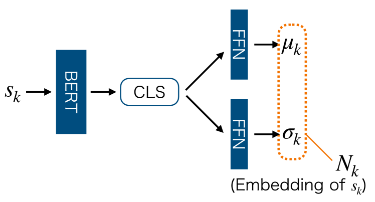
Figure 1: Overview of GaussCSE.

In learning entailment relations, as with word representation by Gaussian embedding, GaussCSE performs learning so that the embedding of a sentence that entails the other sentence has greater variance than the embedding of the sentence to be entailed. To achieve this, we use entailment sentence pairs and increase the corresponding variance of premise (pre) sentences while decreasing it for hypothesis (hyp) sentences in NLI datasets. This is accomplished by training the model to increase $\mbox{sim}(\textit{hyp}||\textit{pre})$ relative to $\mbox{sim}(\textit{pre}||\textit{hyp})$ in accordance with the characteristics of KL divergence described above. Conversely, we decrease $\mbox{sim}(\textit{hyp}||\textit{pre})$ when the premise does not entail the hypothesis, indicating that the pair is not semantically similar. As KL divergence is more sensitive to differences in the mean than the variance, this operation is expected to increase the distance between the distributions of two sentences.

We use contrastive learning with NLI datasets to train the model following Supervised SimCSE. During training, we aim to increase the similarity between positive examples and decrease the similarity between negative examples. We use the following three types of sets for positive and negative examples.

Entailment set

The set of premise and hypothesis pairs labeled with “entailment.” The sentences that are semantically similar are brought to be closer to each other.

Contradiction set

The set of premise and hypothesis pairs labeled with “contradiction.” The sentences that are not entailed are used as negative examples and made apart from each other.

Reversed set

The set of sentence pairs obtained by reversing each sentence pair in the “entailment set.” The sentences whose entailment relation is reversed are used as negative examples in order to increase the variance of premise sentences and decrease the variance of the hypothesis.

Figure 2 illustrates the methods for selecting positive and negative examples in a batch. We compute $\mbox{sim}(\textit{hyp}||\textit{pre})$ for positive and negative examples. Specifically, the similarity of positive and negative examples in the three sets are computed by using a premise sentence $s_{i}$, a hypothesis sentence $s_{i}^{+}$ of the positive example, and a hypothesis sentence $s_{i}^{-}$ of the negative example. The loss function of contrastive learning is:

$$V_{E}=\Sigma_{j=1}^{n}e^{\mathrm{sim}(s_{j}^{+}||s_{i})/\tau},$$

$$V_{C}=\Sigma_{j=1}^{n}e^{\mathrm{sim}(s_{j}^{-}||s_{i})/\tau},$$

$$V_{R}=\Sigma_{j=1}^{n}e^{\mathrm{sim}(s_{j}||s_{i}^{+})/\tau},$$

$$\mathcal{L}=\sum_{i=1}^{n}{-\log\frac{e^{\mathrm{sim}(s_{i}^{+}||s_{i})/\tau}}{V_{E}+V_{C}+V_{R}}},$$ (4)

where $n$ is a batch size, and $\tau$ is a temperature hyperparameter.

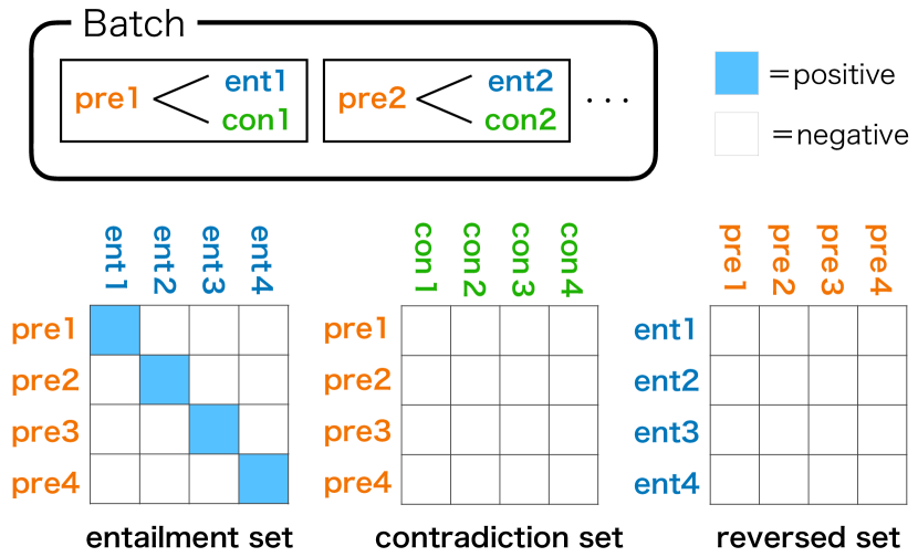
Figure 2:  The methods for selecting positive and negative examples. Each cell in the matrix corresponds to sim(sentence on the vertical axis$||$sentence on the horizontal axis) and is closer to 1 for positive examples and closer to 0 for negative examples. The blue cells denote positive examples, and all the other cells correspond to negative examples.

By performing learning with such a loss function, sentences that are semantically similar are expected to be learned to have close mean vectors. In cases of entailment pairs, it is expected that the variance of the entailing one becomes large and the variance of the entailed one becomes small.

3 Experiment

We validate the effectiveness of GaussCSE through experiments on two tasks: NLI tasks and entailment direction prediction tasks.

3.1 Evaluation tasks

NLI

We evaluated GaussCSE to compare with previous work for recognizing textual entailment. NLI tasks are usually performed as a three-way classification, but it is difficult to execute this using only a similarity measure. Therefore, we performed a two-way classification by collapsing “neutral” and “contradiction” as “non-entailment.” When the value of $\mbox{sim}(\textit{hyp}||\textit{pre})$ is greater than a threshold, it is classified as “entailment”; otherwise classified as “non-entailment.” We used the Stanford NLI (SNLI) Bowman et al. (2015) dataset and SICK Marelli et al. (2014) dataset for evaluation. We used the accuracy (acc.) and area under the precision-recall curve (AUC) as the evaluation metrics. We calculated the threshold with the highest accuracy by the development set by varying the threshold from 0 to 1 in steps of 0.001, and calculated the accuracy using that threshold.

Entailment Direction Prediction

In order to evaluate whether the model can capture the entailment relationship, we performed the task of predicting which sentence entails the other when given two sentences $A$ and $B$ in an entailment relationship. We adopted the similarity-based method (sim) and the variance-based method (var) to determine the direction of entailment. The similarity-based method determines $A$ as entailing one if $\mbox{sim}(\textit{B}||\textit{A})$ is larger than $\mbox{sim}(\textit{A}||\textit{B})$. The variance-based method determines $A$ as entailing one if the variance of embedding of $A$ is larger than $B$. We used only sentence pairs labeled “entailment” in the SNLI and SICK dataset for the entailment direction prediction tasks and accuracy as the evaluation metrics.

3.2 Experimental Setup

We used BERT-base with transformers. We combined SNLI dataset and Multi-Genre NLI (MNLI) dataset Williams et al. (2018) for the training dataset following Gao et al. (2021). Other detailed experimental setups are provided in Appendix A. We conducted experiments with four different loss functions, each with different training data: entailment set alone (ent), entailment and contradiction sets (ent+con), entailment and reversed sets (ent+rev), and all sets (ent+con+rev).

3.3 Result

Table 1 lists the experimental results of the NLI task. The performance of Supervised SimCSE is given as a baseline. Among the four loss functions, ent+con performed the best, which consists of the same training pairs as Supervised SimCSE. Adding contradiction pairs to the negative examples (ent+con, ent+con+rev) improves performance, and outperforms Supervised SimCSE on SICK. On the contrary, adding the reversed set slightly degrades performance. The inverse set consists of semantically similar sentence pairs, and treating such similar sentence pairs as negative examples would have worked adversely in the NLI task.

Table 2 lists the experimental results of entailment direction prediction. By leveraging the reversed set, a remarkably high accuracy of over 97% was achieved on the SNLI dataset. On SICK, ent+rev performed the best, achieving around 72%. Notably, there was a significant difference in performance between the SNLI and SICK datasets. It is probably due to the different characteristics of these datasets such as the differences in the distribution of lengths for sentence pairs. Compared to SICK, SNLI tends to have longer premise sentences than hypothesis sentences, and thus longer sentences are given larger variances for premises have larger variances. In SICK, on the other hand, since the ratio of lengths of premise and hypothesis is almost the same on average, premise and hypothesis sentences did not result in very different variances. It would be the cause for relatively low performance on SICK. Adding reversed set improves the performance of both SNLI and SICK. This demonstrates that using reversed set is useful in reducing the effect of sentence length bias and capturing semantically valid sentence entailment.

4 Conclusion

In this paper, we presented GaussCSE, a Gaussian distribution-based contrastive sentence embedding to handle asymmetric relationships between sentences such as entailment relations. Through experiments on the NLI tasks and the entailment direction prediction tasks, we demonstrated that GaussCSE achieves the same performance as previous methods in NLI tasks, and is able to estimate the direction of entailment relations, which is difficult with point representations. In future work, we will evaluate the performance of GaussCSE in other tasks and analyze the embeddings in more detail, focusing on the distribution of the mean and variance vectors.

	SNLI		SICK
	acc.	AUC	acc.	AUC
Sup-SimCSE	74.96	66.76	86.11	81.41
ent	72.50	61.44	76.50	64.33
ent+con	78.33	72.50	85.21	80.13
ent+swap	70.64	57.57	74.24	57.31
ent+con+swap	77.51	69.33	84.37	78.92

Table 1: Experimental results of the NLI task.

	SNLI		SICK
	sim	var	sim	var
ent	81.65	81.19	63.01	62.44
ent+con	61.56	60.44	61.62	62.18
ent+swap	97.01	97.12	71.23	71.93
ent+con+swap	97.09	97.21	69.22	70.13

Table 2: Experimental results of entailment direction prediction tasks.

Appendix A Detail of Experimental Setup

The dimension of the embedding is 768, the fine-tuning epoch size is 3, the temperature hyperparameter is 0.05, and the optimizer is AdamW Ilya and Frank (2019). These settings are the same as SimCSE Gao et al. (2021). We carry out grid-search of batch size $\in\{64,128,256,512\}$ and learning rate $\in\{1\mathrm{e}{-5},3\mathrm{e}{-5},5\mathrm{e}{-5}\}$ on the SNLI development set, then used the best-performing combination in the in-training evaluation described below. The learning rate is 0 at the beginning and increases linearly to a set value in the final step. The results for each combination are shown in Table 3.

In each experiment, the AUC of the precision-recall curve for the NLI task on the SNLI development set was calculated every 100 training steps, and the model with the best performance was used for the final evaluation on the test set. We conducted experiments with five different random seeds, and their mean was used as the evaluation score.

		Learning Rate
		1e-5	3e-5	5e-5
Batch Size	16	64.39	66.02	67.00
	32	63.21	65.23	65.97
	64	60.79	64.13	65.27
	128	59.93	62.72	63.60
	256	58.86	61.50	62.52

Table 3: AUC of the PR curve for the NLI task for each batch size and learning rate. The values in the table are multiplied by 100.

Appendix B Ratio of Length of Sentence Pairs

Figure 3 shows the ratio of the lengths of the premise and hypothesis sentences for SNLI and SICK. The distribution of SICK is concentrated around 0, indicating that there is no difference in length, on the other hand, SNLI is concentrated in the positive region. This shows that premise sentences tend to be longer than hypothesis on SNLI.

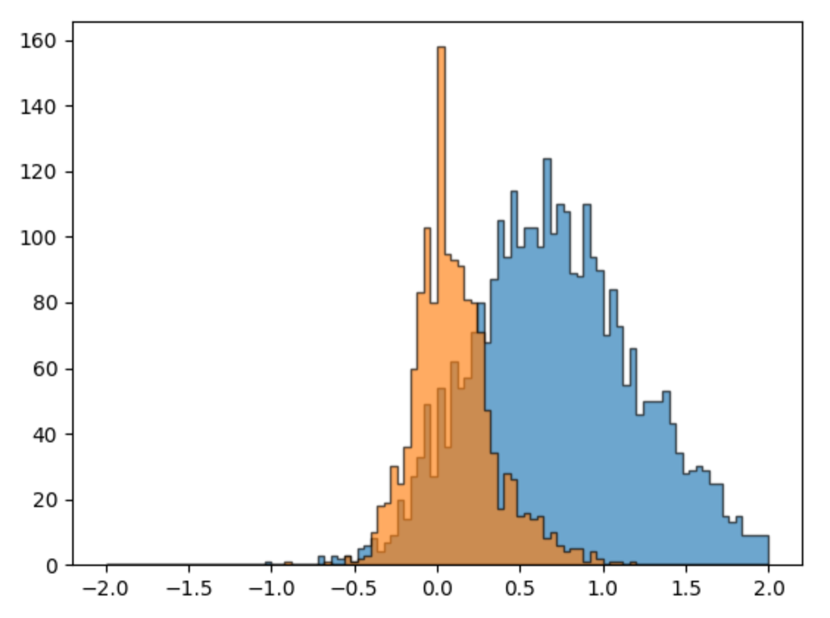
Figure 3: The histogram showing the ratio of the lengths of the premise and hypothesis sentences. The horizontal axis is the ratio of the lengths of the premise and hypothesis (values are taken natural logarithm), and the vertical axis is the number of sentence pairs. The blue graph shows SNLI and the orange shows SICK.

References

- Alm et al. (2005) Cecilia Ovesdotter Alm, Dan Roth, and Richard Sproat. 2005. Emotions from text: Machine learning for text-based emotion prediction. In Proceedings of Human Language Technology Conference and Conference on Empirical Methods in Natural Language Processing, pages 579–586, Vancouver, British Columbia, Canada. Association for Computational Linguistics.
- Bojchevski and Günnemann (2018) Aleksandar Bojchevski and Stephan Günnemann. 2018. Deep Gaussian Embedding of Graphs: Unsupervised Inductive Learning via Ranking. In 6th International Conference on Learning Representations (ICLR).
- Bowman et al. (2015) Samuel R. Bowman, Gabor Angeli, Christopher Potts, and Christopher D. Manning. 2015. A large annotated corpus for learning natural language inference. In Proceedings of the 2015 Conference on Empirical Methods in Natural Language Processing, pages 632–642, Lisbon, Portugal. Association for Computational Linguistics.
- Chuang et al. (2022) Yung-Sung Chuang, Rumen Dangovski, Hongyin Luo, Yang Zhang, Shiyu Chang, Marin Soljacic, Shang-Wen Li, Scott Yih, Yoon Kim, and James Glass. 2022. DiffCSE: Difference-based contrastive learning for sentence embeddings. In Proceedings of the 2022 Conference of the North American Chapter of the Association for Computational Linguistics: Human Language Technologies, pages 4207–4218, Seattle, United States. Association for Computational Linguistics.
- Devlin et al. (2019) Jacob Devlin, Ming-Wei Chang, Kenton Lee, and Kristina Toutanova. 2019. BERT: Pre-training of Deep Bidirectional Transformers for Language Understanding. In Proceedings of the 2019 Conference of the North American Chapter of the Association for Computational Linguistics: Human Language Technologies (NAACL), pages 4171–4186.
- Gao et al. (2021) Tianyu Gao, Xingcheng Yao, and Danqi Chen. 2021. SimCSE: Simple Contrastive Learning of Sentence Embeddings. In Proceedings of the 2021 Conference on Empirical Methods in Natural Language Processing (EMNLP), pages 6894–6910.
- Ilya and Frank (2019) Loshchilov Ilya and Hutter Frank. 2019. Decoupled Weight Decay Regularization. In 7th International Conference on Learning Representations (ICLR).
- Jiang et al. (2022) Ting Jiang, Jian Jiao, Shaohan Huang, Zihan Zhang, Deqing Wang, Fuzhen Zhuang, Furu Wei, Haizhen Huang, Denvy Deng, and Qi Zhang. 2022. PromptBERT: Improving BERT sentence embeddings with prompts. In Proceedings of the 2022 Conference on Empirical Methods in Natural Language Processing, pages 8826–8837, Abu Dhabi, United Arab Emirates. Association for Computational Linguistics.
- Klein and Nabi (2022) Tassilo Klein and Moin Nabi. 2022. SCD: Self-contrastive decorrelation of sentence embeddings. In Proceedings of the 60th Annual Meeting of the Association for Computational Linguistics (Volume 2: Short Papers), pages 394–400, Dublin, Ireland. Association for Computational Linguistics.
- Li et al. (2020) Bohan Li, Hao Zhou, Junxian He, Mingxuan Wang, Yiming Yang, and Lei Li. 2020. On the Sentence Embeddings from Pre-trained Language Models. In Proceedings of the 2020 Conference on Empirical Methods in Natural Language Processing (EMNLP), pages 9119–9130.
- Liu et al. (2020) Dayiheng Liu, Yeyun Gong, Jie Fu, Yu Yan, Jiusheng Chen, Daxin Jiang, Jiancheng Lv, and Nan Duan. 2020. RikiNet: Reading Wikipedia pages for natural question answering. In Proceedings of the 58th Annual Meeting of the Association for Computational Linguistics, pages 6762–6771, Online. Association for Computational Linguistics.
- Liu et al. (2021) Yang Liu, Hua Cheng, Russell Klopfer, Matthew R. Gormley, and Thomas Schaaf. 2021. Effective convolutional attention network for multi-label clinical document classification. In Proceedings of the 2021 Conference on Empirical Methods in Natural Language Processing, pages 5941–5953, Online and Punta Cana, Dominican Republic. Association for Computational Linguistics.
- Luke and Andrew (2015) Vilnis Luke and McCallum Andrew. 2015. Word Representations via Gaussian Embedding. arXiv:1412.6623.
- Marelli et al. (2014) Marco Marelli, Stefano Menini, Marco Baroni, Luisa Bentivogli, Raffaella Bernardi, and Roberto Zamparelli. 2014. A SICK cure for the evaluation of compositional distributional semantic models. In Proceedings of the Ninth International Conference on Language Resources and Evaluation (LREC), pages 216–223.
- Muennighoff (2022) Niklas Muennighoff. 2022. SGPT: GPT Sentence Embeddings for Semantic Search. arXiv.2202.08904.
- Reimers and Gurevych (2019) Nils Reimers and Iryna Gurevych. 2019. Sentence-BERT: Sentence Embeddings using Siamese BERT-Networks. In Proceedings of the 2019 Conference on Empirical Methods in Natural Language Processing and the 9th International Joint Conference on Natural Language Processing (EMNLP-IJCNLP), pages 3982–3992.
- Shizhu et al. (2015) He Shizhu, Liu Kang, Ji Guoliang, and Zhao Jun. 2015. Learning to Represent Knowledge Graphs with Gaussian Embedding. Proceedings of the 24th ACM International on Conference on Information and Knowledge Management.
- Williams et al. (2018) Adina Williams, Nikita Nangia, and Samuel Bowman. 2018. A broad-coverage challenge corpus for sentence understanding through inference. In Proceedings of the 2018 Conference of the North American Chapter of the Association for Computational Linguistics: Human Language Technologies, Volume 1 (Long Papers), pages 1112–1122.
- Wu et al. (2022) Bohong Wu, Zhuosheng Zhang, Jinyuan Wang, and Hai Zhao. 2022. Sentence-aware contrastive learning for open-domain passage retrieval. In Proceedings of the 60th Annual Meeting of the Association for Computational Linguistics (Volume 1: Long Papers), pages 1062–1074, Dublin, Ireland. Association for Computational Linguistics.
- Zhang et al. (2020) Yan Zhang, Ruidan He, Zuozhu Liu, Kwan Hui Lim, and Lidong Bing. 2020. An unsupervised sentence embedding method by mutual information maximization. In Proceedings of the 2020 Conference on Empirical Methods in Natural Language Processing (EMNLP), pages 1601–1610, Online. Association for Computational Linguistics.