HJB based online safe reinforcement learning for state-constrained systems

Abstract

This paper proposes a safe reinforcement learning(RL) algorithm that solves the constrained optimal control problem for continuous-time nonlinear systems with uncertain dynamics. We formulate the safe RL problem as minimizing a Lagrangian involving the cost functional and a user-defined barrier Lyapunov function(BLF) encoding the state constraints. We show that the analytical solution obtained by the corresponding Hamilton-Jacobi-Bellman(HJB) equations involves an expression for the Lagrange multiplier, which includes unknown terms arising from the system uncertainties. However, the naive estimation of the aforementioned Lagrange multiplier may lead to safety constraint violations. To obviate this challenge, we propose a novel Actor-Critic-Identifier-Lagrangian(ACIL) algorithm that learns optimal control policies from online data without compromising safety. The safety and boundedness guarantees are proved for the proposed algorithm. Subsequently, we compare the performance of the proposed ACIL algorithm against existing offline/online RL methods in a simulation study.

I Introduction

Reinforcement learning (RL) has been recently used in control theory to solve optimal control problems under system uncertainties. RL algorithms provide a way to combine the two fields of control theory, namely- adaptive control and optimal control. Leveraging the general framework of RL, the control community has seen reasonable success in the literature for discrete-time and continuous-time systems under both deterministic and stochastic settings (see [36, 7, 29] for examples in the continuous-time domain, and [8, 33] for discrete-time domain). Despite its successes, the real-world implementation of such learning-based controllers on safety-critical systems is still challenging due to the lack of provable safety guarantees of on-policy RL algorithms. Specifically, due to inadequate knowledge of the system dynamics during training, on-policy RL algorithms tend to naively explore the state space without considering safety objectives. Thus solely relying on on-policy RL-based controllers may lead to safety violations. To alleviate this challenge, the field of safe reinforcement learning (safe RL) emerged, and researchers are actively seeking to bolster RL algorithms with safety guarantees.

In the context of safe RL-based control, mathematically, “safety” often refers to the satisfaction of user-defined constraints during training and deployment. Specifically, safety formulations in dynamical systems often seek to ensure invariance of constraint sets on state or control action [9]. Based on this mathematical formulation, some common approaches to ensuring safety for RL-based control include - using control barrier functions (CBF) [4, 3], model predictive control (MPC) [22, 38, 6], temporal logic (TL) specifications [14, 2], and using Gaussian processes [16, 12] to name a few. Control barrier functions and its Lyapunov-like counterpart - barrier Lyapunov functions (BLF) [34] provide a method for studying the forward invariance of constraint sets through a Lyapunov-like analysis, without the necessity to compute the system trajectories.

Another school of thought in solving optimal control problems under constraints is utilizing numerical approaches (see e.g. [18, 17] and [31] for a detailed survey). These approaches provide close-to optimal solutions for the desired objective functional under user-defined state and actuation constraints. However, these methods usually assume the complete knowledge of the system and are generally trained offline.

To enable adaptation to parametric uncertainties online, several online on-policy RL algorithms have been detailed in the literature [36, 7, 35, 20] aiming to solve the optimal control problem in the continuous-time deterministic setting. Inspired by these methods, numerous safe RL algorithms have been proposed. These include using barrier transformation based techniques [37, 26] which transform the constrained state into an unconstrained state and subsequently apply approximate dynamic programming techniques. Another class of methods augment the barrier Lyapunov functions in the cost functional of the optimal control problem [27, 13]. While the barrier transformation methods can only be applied if the state constraints are box constraints, the methods in [27, 13] rely on the assumption that the resulting value function is continuously differentiable (see [26]) which may not hold for some systems and safe sets. The authors of [15] proposed an online RL algorithm using a so called “safeguarding controller” which uses the gradient of a user-defined barrier Lyapunov function to modify the optimal control law in a minimally invasive fashion to ensure safety. The aforementioned method uses a gain $c_{b}$ to trade-off the safety and stability objectives.

One promising method for computing safe RL policies can be considered by minimizing a desired cost functional with respect to (w.r.t.) a constraint on the time derivative of a user-defined candidate BLF or a candidate CBF. The optimal control law for the formulation mentioned above may be found using Karush-Kuhn-Tucker conditions (see [1]) along with an optimal Lagrange multiplier dependent on the state. However, under such methods, the optimal Lagrange multiplier includes terms of the uncertain drift dynamics and optimal value function, which is difficult to compute analytically. While the authors of [1] proposed an offline method (safe Galerkin successive approximation) to learn the optimal control policy, we show that the naive extension to an online algorithm fails to ensure the safety of the underlying system under some non-trivial scenarios.

To alleviate this challenge, in this paper, we detail an online on-policy RL algorithm involving a novel online estimator for the optimal Lagrange multiplier that approximately solves the optimal control problem for a class of deterministic continuous-time nonlinear systems with parametric uncertainties, under user-defined state constraints. The proposed Actor-Critic-Identifier-Lagrangian (ACIL) algorithm extends the approach by [20] to the constrained setting by including this novel online Lagrange multiplier estimate. The primary difference between the proposed method and [15] is that while the gain for the safeguarding controller in [15] is held constant, the Lagrange multiplier in our work varies according to the safety requirements of the current state. Consequently, we observe better performance in the sense of total cost accrued (which we demonstrate on some numerical simulations). To the best of our knowledge, such an online estimator for the Lagrange multiplier and the constraint on the time derivative of BLF has not been reported in the literature.

I-A Contribution

The contribution of this paper is three-fold. First, we formulate the safety problem of RL based optimal control as the minimization of the desired cost functional subject to a constraint involving the time derivative of the BLF. We subsequently formulate the equivalent Lagrangian functional and develop optimal control law for the constrained system via the Karush-Kuhn-Tucker conditions. Second, we show that the naive estimation of the Lagrange multiplier fails to ensure safety of the underlying system. Third, we propose a novel estimator for the Lagrange multiplier under parametric uncertainties and show that the same is sufficient to ensure safety of the RL agent. Subsequently we extend the Actor-Critic-Identifier algorithm from [7] and [20] to safely learn the optimal control policies online. To demonstrate the efficacy of the proposed controller, we perform simulation studies on two systems with complex state constraints and compare our results with similar approaches in the literature.

I-B Notation

We use $\|\cdot\|$ to denote the Euclidean norm for the vectors and the corresponding induced norm for matrices. We use $\nabla_{x}$ to denote the gradient operator with respect to the state $x$ yielding a column vector. Let $\mathbb{I}_{n}$ denote the $n\times n$ identity matrix. Let $\mathcal{L}_{\infty}$ denote the set of all bounded signals. We denote the set of all natural numbers upto and including $n$ by $\mathbb{N}_{n}$. We define $\overline{\|(\cdot)\|}\triangleq\sup_{x\in\text{Int}(\mathcal{C})}\|(\cdot)\|$ for a continuous mapping $(\cdot):\mathcal{C}\rightarrow\mathbb{R}^{q}$. $\lambda_{\min}(A)$ denotes the minimum eigenvalue of the square matrix $A$.

II Problem Formulation

In this paper, we solve the state-constrained optimal control problem for a class of nonlinear systems

$$\dot{x}=f(x,\theta)+g(x)u,\;\;\;x(t_{0})=x_{0},$$ (1)

where $x(t)\in\mathbb{R}^{n}$ and $u(t)\in\mathbb{R}^{m}$ are the state and control vectors respectively; $f:\mathbb{R}^{n}\times\mathbb{R}^{p}\rightarrow\mathbb{R}^{n}$ and $g:\mathbb{R}^{n}\rightarrow\mathbb{R}^{n\times m}$ are Lipschitz continuous functions and $\theta\in\Theta\subset\mathbb{R}^{p}$ is an unknown parameter vector. We consider the drift dynamics $f(x,\theta)$ to be linear in the parameter $\theta$, i.e.

$$f(x,\theta)=Y(x)\theta,$$ (2)

where we call the continuous function $Y:\mathbb{R}^{n}\rightarrow\mathbb{R}^{n\times p}$ as the regressor. We assume the complete knowledge of the functions $Y(x)$ and $g(x)$, and state $x$ is considered to be measurable. The objective of the safe RL agent is to choose a control policy $u(t)\;\;\forall\;t\in[t_{0},\infty)$, to minimize the cost functional

$$J(x,t_{0})=\int_{t_{0}}^{\infty}r(x,u)dt,$$ (3)

where the positive semi-definite function $r:\mathbb{R}^{n}\times\mathbb{R}^{m}\rightarrow\mathbb{R}$ is called the instantaneous cost function. In the present work, we solve the optimal regulation problem for the system in (1) using the cost function defined as

$$r(x,u)\triangleq Q(x)+\frac{1}{2}u^{T}Ru,$$ (4)

where $Q:\mathbb{R}^{n}\rightarrow\mathbb{R}$ is positive semi-definite function on the state with $Q(0)=0$ and $R\in\mathbb{R}^{m\times m}$ is a positive definite control effort weight matrix. In addition to minimizing the cost functional in (3), the control policy must also, ensure the safety of the system formulated as ensuring the forward invariance [9] of a user-defined compact set $\mathcal{C}\subset\mathbb{R}^{n}$ containing the origin, i.e.,

$$x(t_{0})\in\mathcal{C}\implies x(t)\in\mathcal{C}\;\;\forall\;t\in[t_{0},\infty).$$ (5)

For the ease of exposition, we define the sets $\partial\mathcal{C}$ and $\text{Int}(\mathcal{C})$ to be the boundary and the interior of the set $\mathcal{C}$ respectively.

To ensure satisfaction of (5) online, we reformulate the set membership constraint to an equivalent formulation using a barrier Lyapunov function(BLF) as discussed in the subsequent section.

II-A Constraint reformulation using barrier Lyapunov functions

We define a barrier Lyapunov function over the constraint set $\mathcal{C}$ as follows

Definition 1 (Barrier Lyapunov function)

A positive definite continuously differentiable function $B_{f}(x):\mathcal{C}\rightarrow\mathbb{R}$ satisfying $B_{f}(0)=0$, $B_{f}(x)>0\;\;\forall\;x\in\mathcal{C}/\{0\}$, and $\lim_{x\rightarrow\partial\mathcal{C}}B_{f}(x)=\infty$ is called a barrier Lyapunov function(BLF), if its time derivative along the system trajectories is negative semi-definite, i.e., $\dot{B}_{f}(x)\leq 0\;\;\forall\;x\in\text{Int}(\mathcal{C})$.

We now use the definition of BLF to state the following Lemma which relates the concepts of BLF and forward invariance of $\mathcal{C}$.

Lemma 1

The existence of a barrier Lyapunov function $B_{f}$ over the domain $\mathcal{C}$ for a system $\dot{x}=f(x,\theta)+g(x)u$, implies that the compact set $\mathcal{C}$ is forward invariant[34, Lemma 1],

From Lemma 1 we can infer that provided a user-defined BLF $B_{f}$ and a control policy $u(t)$ satisfying $\dot{B}_{f}|_{u(t)}\leq 0$, the control law $u(t)$ also satisfies the constraint (5). We can thus reformulate the state constraint (5) to an equivalent formulation using BLF $B_{f}$ as

$$\nabla_{x}B_{f}(x)^{T}[f(x,\theta)+g(x)u]\leq 0\;\;\forall\;t\in[t_{0},\infty),$$ (6)

where the time dependence of the signals have been suppressed for notational brevity. We would utilize this constraint reformulation to obtain a closed-form solution for the original constrained optimal control problem. Specifically, we construct a user-defined candidate BLF $B_{f}(x)$ in such a way that the following assumption holds

Assumption 1

$\exists\;\gamma\in\mathbb{R}_{>0}$ satisfying $\gamma\|\nabla_{x}B_{f}(x)\|\geq B_{f}(x)\;\;\;\forall\;x\in\text{Int}(\mathcal{C})$.

The knowledge of the constant $\gamma$ is used in Section V for obtaining the largest invariant subset of $\mathcal{C}$. We provide a few examples of the constant $\gamma$ satisfying Assumption 1 for some commonly used BLFs in Table I.

TABLE I: Value of $\gamma$ for some BLFs

Safe set ($\mathcal{C}$)	Candidate BLF ($B_{f}(x)$)	$\gamma$
$\{x\in\mathbb{R}^{n}:\|x\|\leq\beta\}$	$\ln(\frac{\beta^{2}}{\beta^{2}-x^{T}x})$	$0.5\beta$
$\{x\in\mathbb{R}^{n}:|x_{i}|\leq a_{i}\;\forall\;i\in\mathbb{N}_{n}\}$	$\sum_{i}\ln(\frac{a_{i}^{2}}{a_{i}^{2}-x_{i}^{2}})$	$0.5\max_{i}(a_{i})$

We now state the main problem formulation for the present work, the BLF-based state-constrained optimal control problem (BLF-COCP)

Problem 1 (BLF-COCP)

$$\min_{u(\tau)\;\;\forall\;\tau\in[t_{0},\infty)}\hskip 2.0pt \int_{t_{0}}^{\infty}Q(x(\tau))+u(\tau)^{T}Ru(\tau)d\tau,$$ (7a)

s.t. $$\nabla_{x}B_{f}^{T}[f(x,\theta)+g(x)u(\tau)]\leq 0,$$ (7b)

$$\dot{x}=f(x,\theta)+g(x)u\;\;\forall\;\tau\in[t_{0},\infty),$$ (7c)

$$B_{f}(x(t_{0}))<\infty.$$ (7d)

II-B Existence of a feasible solution

We will now show that there exists at least one feasible control policy that satisfies the constraints of Problem 1. In order to do so, we make the following assumptions on the control effectiveness matrix $g(x)$ and the candidate BLF $B_{f}(x)$

Assumption 2

The control effectiveness matrix $g(x)$ satisfies $\lambda_{\min}\big{(}R_{g}(x)\big{)}>l_{g}\;\text{and}\;\|R_{g}(x)\|\leq\overline{R}_{g}\;\;\forall\;x\in\mathcal{C}$, where $R_{g}(x):\mathbb{R}^{n}\rightarrow\mathbb{R}^{n\times n}$ is defined as $R_{g}(x)\triangleq g(x)R^{-1}g^{T}(x)$ and $\overline{R}_{g},l_{g}\in\mathbb{R}_{>0}$ are computable positive constants.

Assumption 3

The control matrix $g(x)$ and the barrier Lyapunov function $B_{f}(x)$ satisfy the condition $\nabla_{x}B_{f}^{T}(x)g(x)\neq 0\;\;\forall\;x\in\text{Int}(\mathcal{C})$.

We now state the following Lemma

Lemma 2

Under Assumption 3, there exists a control policy $u_{safe}(x)=-[\nabla_{x}B_{f}^{T}(x)g(x)]^{\dagger}\nabla_{x}B_{f}^{T}(x)f(x,\theta)$, where $\dagger$ denotes the Moore-Penrose pseudoinverse [11]; such that $\dot{B}_{f}|_{u_{safe}}=0\;\;\forall\;x\in\text{Int}(\mathcal{C})$.

Proof:

Proof We compute the time derivative of the BLF $B_{f}(x)$ as

$$\dot{B}_{f}(x)|_{u_{safe}}=\nabla_{x}B_{f}^{T}[f(x,\theta)+g(x)u_{safe}].$$ (8)

Substituting the expression for the proposed control policy $u_{safe}$ we have

$$\dot{B}_{f}(x)=\nabla_{x}B_{f}^{T}f-\nabla_{x}B_{f}^{T}g[\nabla_{x}B_{f}^{T}g]^{\dagger}\nabla_{x}B_{f}^{T}f=0,$$ (9)

which satisfies the constraint of Problem 1.

∎

From Lemma 2, we can conclude that there exists atleast one feasible control policy satisfying the constraints of Problem 1. We will now solve Problem 1 using approximate dynamic programming in the next section.

III Constrained optimal control based on approximate dynamic programming

To solve the constrained optimal control problem we define the Lagrangian functional as

$$L(x(t_{0}),\lambda(x(t_{0})))=\int_{t_{0}}^{\infty}\Big{(}r(x,u)+\lambda(x)\frac{dB_{f}}{dt}\Big{)}d\tau,$$ (10)

where $\lambda(x):\mathbb{R}^{n}\rightarrow\mathbb{R}$ is the Lagrange multiplier. Since we consider the infinite horizon control problem with autonomous system dynamics and stationary state constraints, the Lagrange multiplier is not an explicit function of time. Utilizing Bellman’s optimality principle [5], and following the analysis from [25, Section 6.3] we write the Hamilton-Jacobi-Bellman (HJB) equation for the constrained problem as

$$0=\min_{\begin{subarray}{c}u(t),\lambda(x)\end{subarray}} \Big{[}r(x,u)+\lambda\nabla_{x}B_{f}^{T}[f(x,\theta)+g(x)u]$$ (11)

$$+\nabla_{x}L^{*T}[f(x,\theta)+g(x)u]\Big{]}\;\;\forall\;x\in\mathbb{R}^{n}.$$

We now derive the optimal control law under the assumption that we know the true value function $L^{*}(\cdot)$. We would subsequently approximate $L^{*}(\cdot)$ by a universal function approximator like a neural network to make the control law implementable. We observe that, provided the knowledge of the value function $L^{*}(\cdot)$ the optimization problem in (11) is convex in the decision variable $u(t)$. Thus, the optimal solution can be obtained by the Karush-Kuhn-Tucker (KKT) conditions [10, Section 5.3.3]

$$\frac{\partial}{\partial u}\Big{[}r(x,u)+\lambda\nabla_{x}B_{f}^{T}(f+gu)+\nabla_{x}L^{*T}(f+gu)\Big{]}=0,$$ (12a)

$$\lambda^{*}(x(t))\nabla_{x}B_{f}^{T}(f+gu^{*})=0,$$ (12b)

$$\lambda^{*}(x(t))\geq 0\;\;\forall\;t\in\mathbb{R}_{\geq t_{0}}.$$ (12c)

Remark 1

While we enjoy the convexity afforded to us by considering a cost function quadratic in $u$, control-affine system dynamics, and assuming a structure on the value function; the overall problem in Problem 1 is not a convex optimization problem due to the presence of the value function.

Using the first order condition in (12a) and the instantaneous cost function from (4), we can write the optimal control law as

$$u^{*}(x)=-R^{-1}g^{T}(x)[\nabla_{x}L^{*}(x)+\lambda^{*}(x)\nabla_{x}B_{f}(x)].$$ (13)

Substituting (13) in the complementary slackness condition (12b) and using the condition on the dual constraint (12c) we have the optimal Lagrange multiplier (cf. [1]) as

$$\lambda^{*}(x)=\begin{cases}\max\Big{(}\frac{C_{s}^{*}(x)}{R_{bf}(x)},0\Big{)},&\text{if }\nabla_{x}B_{f}(x)\neq 0,\\ 0,&\text{otherwise}.\\ \end{cases}$$ (14)

where $R_{bf}(x)\triangleq\nabla_{x}B_{f}(x)^{T}R_{g}(x)\nabla_{x}B_{f}(x)$, $R_{g}(x)$ was defined in Assumption 2 and

$$C_{s}^{*}(x)\triangleq\nabla_{x}B_{f}(x)^{T}f(x,\theta)-\nabla_{x}B_{f}(x)^{T}R_{g}(x)\nabla_{x}L^{*}.$$ (15)

Lemma 3

Under the optimal control law in (13) the set $\mathcal{C}$ is forward invariant for the system in (1).

Proof:

Proof Consider the positive definite candidate Lyapunov function $B_{f}(x)$. The time derivative of the same along the system trajectories is given by $\dot{B}_{f}(x)=\nabla_{x}B_{f}(x)^{T}[f(x,\theta)+g(x)u^{*}(x)]$. Substituting $u^{*}(x)$ and $\lambda^{*}(x)$ from (13) and (14) respectively, we write

$$\dot{B}_{f}(x)=\begin{cases}C_{s}^{*}(x),&\text{if }C_{s}^{*}(x)\leq 0\text{ and }\nabla_{x}B_{f}(x)\neq 0,\\ 0,&\text{otherwise}.\\ \end{cases}$$

We observe that the time derivative of the BLF $B_{f}(x)$ can be bound as $\dot{B}_{f}(x)\leq 0.$ We thus conclude that $B_{f}(x)$ is a valid Barrier Lyapunov function. Invoking Lemma 1, we can show that the set $\mathcal{C}$ is forward invariant for the system in (1). ∎

Remark 2

The term $C_{s}^{*}(x)$ is the derivative of the BLF under the control law without the influence of the safety inducing term $\lambda^{*}(x)\nabla_{x}B_{f}(x)$. If $C_{s}^{*}(x)$ is negative at a particular state $x$, then the value function component of the control law suffices to ensure system safety at $x$ and thus the safety inducing term is 0. On the other hand, when $C_{s}^{*}(x)$ is positive, the safety inducing term steps in and applies a non-zero control effort to make $\dot{B}_{f}(x)\leq 0$ at state $x$.

Since we don’t know $L^{*}(x)$ and $\theta$, the $C_{s}^{*}(\cdot)$ and consequently $\lambda^{*}(\cdot)$ are unimplementable. In the subsequent section, we propose an online estimation technique to approximate these terms.

IV Online estimation of the constrained optimal controller

Since the value function $L^{*}(x)$ is unknown and difficult to compute analytically, we use a single-layer neural network defined over a compact set $\mathcal{D}\subset\mathbb{R}^{n}$ containing the origin such that $\mathcal{C}\subseteq\mathcal{D}$, to approximate $L^{*}(x)$. To that effect, we consider a continuously differentiable user-defined basis function $\phi(x):\mathcal{D}\rightarrow\mathbb{R}^{b}$ with $\phi(0)=0$ and $\nabla_{x}\phi(0)=0$. We parameterize the value function $L^{*}(x)$ as

$$L^{*}(x)=W^{T}\phi(x)+\epsilon(x),$$ (16)

where $W\in\mathbb{R}^{b}$ is the unknown weight vector, and $\epsilon:\mathcal{D}\rightarrow\mathbb{R}$ is the function reconstruction error for the proposed neural network.

Lemma 4

The neural network function reconstruction error $\epsilon(x)$ and its derivative w.r.t. state are bounded as $\|\epsilon(x)\|\leq\overline{\epsilon}$ and $\|\nabla_{x}\epsilon(x)\|\leq\overline{\epsilon}_{d}\;\;\forall\;x\in\mathcal{D}$ , where $\overline{\epsilon},\overline{\epsilon}_{d}\in\mathbb{R}_{>0}$ are positive constants. Additionally these bounds can be made arbitrarily close to zero by choosing an appropriate basis function $\phi$ and increasing the number of neurons considered [23].

In addition to not knowing the value function, we also consider the drift dynamics in (2) to be parameterized by an unknown parameter $\theta$, which, we estimate by $\hat{\theta}(t)\in\mathbb{R}^{p}$. Thus the estimated drift dynamics is defined as

$$\hat{f}(x,\hat{\theta})=Y(x)\hat{\theta}.$$ (17)

We estimate the unknown weight vector $W$ in (16) by two signals $\hat{W}_{a}(t),\hat{W}_{c}(t)\in\mathbb{R}^{b}\;\;\forall\;t\geq t_{0}$ for the control action and value function estimate respectively. We can write the estimate for the value function from (16) and control law from (13) as

$$\hat{L}(x,\hat{W}_{c})=\hat{W}_{c}^{T}\phi(x),$$ (18)

$$\hat{u}(x,\hat{W}_{a},\hat{\theta})= -R^{-1}g^{T}(x)[\nabla_{x}\phi(x)^{T}\hat{W}_{a}$$ (19)

$$+\hat{\lambda}(x,\hat{W}_{a},\hat{\theta})\nabla_{x}B_{f}(x)],$$

respectively, where $\hat{\lambda}(x,\hat{W}_{a},\hat{\theta}):\mathbb{R}^{n}\times\mathbb{R}^{b}\times\mathbb{R}^{p}\rightarrow\mathbb{R}$ is an online estimate of the Lagrange multiplier in (14). In the subsequent section we detail an algebraic expression for $\hat{\lambda}(\cdot)$.

We now propose an online on-policy RL approach consisting of the following components

• Actor - The update law for $\hat{W}_{a}$ for estimating the control law, aiming to minimize the actor parameter estimation error $\tilde{W}_{a}(t)\triangleq W-\hat{W}_{a}(t)$.

• Critic - The update law for $\hat{W}_{c}$ for estimating the value function, aiming to minimize the critic parameter estimation error $\tilde{W}_{c}(t)\triangleq W-\hat{W}_{c}(t)$.

• Identifier - The update law for $\hat{\theta}$ for estimating the system drift dynamics, aiming to minimize the parameter estimation error $\tilde{\theta}(t)\triangleq\theta-\hat{\theta}(t)$.

• Lagrangian - The algebraic expression for $\hat{\lambda}$ estimating the optimal Lagrange multiplier, aiming to minimize the error $\tilde{\lambda}(x)\triangleq\lambda^{*}(x)-\hat{\lambda}(x)$.

We now detail each of the components of the proposed “Actor-Critic-Identifier-Lagrangian (ACIL) ” algorithm in the following subsections.

IV-A Challenges with estimating Lagrange multiplier using the $\max$ function

We now show that the naive Lagrange multiplier estimate obtained by replacing the unimplementable terms in $\lambda^{*}(\cdot)$ with their corresponding estimates, i.e.

$$\hat{\lambda}_{n}(x,\hat{W}_{a},\hat{\theta})=\begin{cases}\max\Big{(}\frac{\hat{C}_{s}(x,\hat{W}_{a},\hat{\theta})}{R_{bf}(x)},0\Big{)},&\text{if }\nabla_{x}B_{f}(x)\neq 0,\\ 0,&\text{otherwise},\\ \end{cases}$$ (20)

where

$$\hat{C}_{s}(x,\hat{W}_{a},\hat{\theta}) \triangleq\nabla_{x}B_{f}(x)^{T}f(x,\hat{\theta})$$ (21)

$$-\nabla_{x}B_{f}(x)^{T}R_{g}(x)\nabla_{x}\phi(x)^{T}\hat{W}_{a},$$

is the online estimate of $C_{s}^{*}(\cdot)$; may fail to ensure the safety of the system. To show this, we consider the candidate Lyapunov function $B_{f}(x)$. Computing the time derivative of the same along the system trajectories under control (19) with the estimate $\hat{\lambda}_{n}$, we have

$$\dot{B}_{f}=C_{s}^{*}+\nabla_{x}B_{f}^{T}R_{g}(\nabla_{x}\epsilon+\nabla_{x}\phi^{T}\tilde{W}_{a})-\max(\hat{C}_{s},0).$$ (22)

During the initial phases of RL training, the estimate $\hat{C}_{s}(\cdot)$ may be far off from the ground-truth $C_{s}^{*}(\cdot)$. There may exist some non-trivial situations where $C_{s}^{*}>0$ while $\hat{C}_{s}<0$. In such a case, the $\dot{B}_{f}>0$ and consequently the BLF grows indefinitely. Under such a case, the RL agent fails to ensure safety of the system.

IV-B Approximation of Lagrange multiplier using softplus function

To alleviate this challenge, we propose a novel online Lagrange multiplier estimate inspired by the developments in the machine learning community. Specifically, expression for $\lambda^{*}(x)$ in (14) involves the maximum operator, which closely resembles the Rectified Linear Unit (ReLU) activation function [28] in the machine learning parlance. However, the ReLU function is non-differentiable at zero. To account for this, “softplus” function $\sigma:\mathbb{R}\rightarrow\mathbb{R}$ was introduced in [28] defined by

$$\sigma(z)\triangleq k\ln(1+\exp(z/k)),$$ (23)

where $k\in\mathbb{R}_{>0}$ is a user-defined gain term. We provide the plot for the softplus function for various values of $k$ in Fig. 1. We observe that as the value of the gain $k$ decreases, the softplus function becomes a better approximation for the ReLU function.

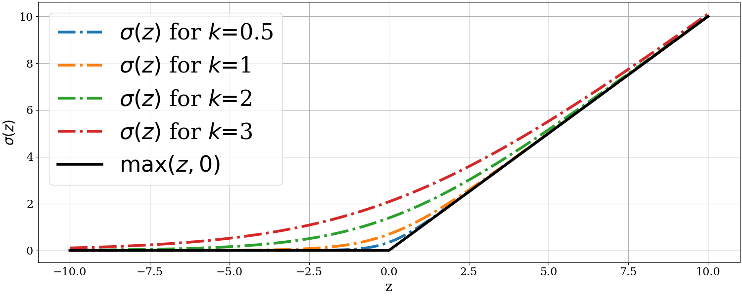
Figure 1: Softplus function

The softplus function has a few desirable properties that are useful in the context of developing online estimators for the optimal Lagrange multiplier, which we encapsulate in the following two Lemmas.

Lemma 5

The function $\sigma(z)$, its first derivative $\sigma{{}^{\prime}}(z)$, and its second derivative $\sigma{{}^{\prime\prime}}(z)$ satisfy $\max(z,0)-\sigma(z)\leq 0$, $0\leq\sigma{{}^{\prime}}(z)\leq 1$, $0\leq\sigma{{}^{\prime\prime}}(z)\leq\frac{1}{4k},\;\;\forall\;z\in\mathbb{R}$.

Lemma 6

The function $f_{\sigma}:(0,\infty)\rightarrow\mathbb{R}$ defined as $f_{\sigma}(z)\triangleq\sigma(c/z)z$, where $c\in\mathbb{R}_{>0}$ is a constant, can be upper-bound as $f_{\sigma}(z)\leq k\ln(2)z+c\;\;\forall\;z\in(0,\infty)$, where $k$ is the gain for the softplus function defined in (23) .

We design an estimate $\hat{\lambda}(\cdot)$ to the optimal Lagrange multiplier $\lambda^{*}(\cdot)$ from (14) as

$$\hat{\lambda}(x,\hat{W}_{a},\hat{\theta})=\sigma\Big{(}\frac{\hat{C}_{s}(x,\hat{W}_{a},\hat{\theta})}{R_{bf}(x)+k_{sb}}\Big{)}+k\varsigma,$$ (24)

where $\varsigma\triangleq\frac{2\ln(2)\overline{R}_{g}}{l_{g}}+1$ is a computable positive constant, $k_{sb}\in\mathbb{R}_{>0}$ is a user-defined constant. Ideally, the constants $k$ and $k_{sb}$ must be chosen very close to zero to better approximate the structure of $\lambda^{*}(\cdot)$. We show the safety guarantees of the proposed controller in Section V.

IV-C Actor-Critic design based on simulation of experience

We now extend the Actor-Critic design from [20] involving a “simulation of experience” paradigm to the training of online estimators for the value function of constrained optimal control problem. The objective of the critic component of the algorithm is to minimize the Bellman Error(BE) $\delta:\mathbb{R}^{n}\times\mathbb{R}^{b}\times\mathbb{R}^{b}\times\mathbb{R}^{p}\rightarrow\mathbb{R}$ defined as

$$\delta(x,\hat{W}_{c},\hat{W}_{a},\hat{\theta})\triangleq r(x,u(x,\hat{W}_{a},\hat{\theta}))+\big{(}\nabla_{x}\hat{L}(x,\hat{W}_{c})$$ (25)

$$+\hat{\lambda}(x,\hat{W}_{a},\hat{\theta})\nabla_{x}B_{f}(x)\big{)}^{T}[f(x,\hat{\theta})+g(x)u(x,\hat{W}_{a},\hat{\theta})],$$

which is equivalent to the error in estimating (11) by the corresponding estimates for the ideal parameters. The authors of [20] observed that the BE can be evaluated independent to the state trajectory and proposed to evaluate the BE at so called “Bellman extrapolation points”, to enable a virtual exploration of the state space. In this paper, we make a slight modification to that framework by considering the set of functions $\{X_{i}:\mathbb{R}^{n}\times[t_{0},\infty)\rightarrow\mathcal{C}\}_{i=1}^{N}$, such that each $X_{i}(\cdot)$ maps the current state to a point $x_{i}\in\mathcal{C}$. Thus the critic evaluates the BE at each extrapolation point

$$\delta_{i}(x_{i},\hat{W}_{c},\hat{W}_{a},\hat{\theta})\triangleq r(x_{i},u(x_{i},\hat{W}_{a},\hat{\theta}))+\big{(}\nabla_{x}\hat{L}(x_{i},\hat{W}_{c})$$ (26)

$$+\hat{\lambda}(x_{i},\hat{W}_{a},\hat{\theta})\nabla_{x}B_{f}(x_{i})\big{)}^{T}[f(x_{i},\hat{\theta})+g(x_{i})u(x_{i},\hat{W}_{a},\hat{\theta})],$$

where $x_{i}(t)=X_{i}(x(t),t)\;\;\forall\;i\in\mathbb{N}_{N}$. The critic uses the information of the gradient of the Bellman Errors w.r.t. $\hat{W}_{c}$ to update its estimate of the neural network parameter. Specifically, the critic computes the signals $\omega(t),\omega_{i}(t)\in\mathbb{R}^{b}\;\forall\;i\in\mathbb{N}_{N}$ defined as $\omega(t)\triangleq\frac{\partial}{\partial\hat{W}_{c}}\delta(\cdot)$ and $\omega_{i}(t)\triangleq\frac{\partial}{\partial\hat{W}_{c}}\delta_{i}(\cdot)$ respectively. The critic subsequently uses the BEs computed in (25) and (26) to improve the estimate $\hat{W}_{c}(t)$ using a recursive least squares-based update law (RLS update law) as

$$\dot{\hat{W}}_{c}(t)=-\eta_{c1}\Gamma(t)\frac{\omega(t)}{\rho(t)^{2}}\delta(\cdot)-\frac{\eta_{c2}}{N}\Gamma(t)\sum_{i=1}^{N}\frac{\omega_{i}(t)}{\rho_{i}(t)^{2}}\delta_{i}(\cdot),$$ (27)

where $\rho(t)\triangleq\sqrt{1+\nu\omega(t)^{T}\Gamma(t)\omega(t)}$ and $\rho_{i}(t)\triangleq\sqrt{1+\nu\omega_{i}(t)^{T}\Gamma(t)\omega_{i}(t)}$ are normalizing factors with $\nu,\eta_{c1},\eta_{c2}\in\mathbb{R}_{>0}$ being user-defined positive gains. The least squares gain matrix $\Gamma(t)\in\mathbb{R}^{b\times b}$ in (27) is updated according to the update law

$$\dot{\Gamma}(t) =\beta\Gamma(t)-\eta_{c1}\Gamma(t)\frac{\omega(t)\omega(t)^{T}}{\rho^{2}(t)}\Gamma(t)$$ (28)

$$-\frac{\eta_{c2}}{N}\Gamma(t)\sum_{i=1}^{N}\frac{\omega_{i}(t)\omega_{i}(t)^{T}}{\rho_{i}^{2}(t)}\Gamma(t),\;\Gamma(t_{0})=\Gamma_{0},$$

where $\beta\in\mathbb{R}_{>0}$ is a constant forgetting factor and $\Gamma_{0}\in\mathbb{R}^{b\times b}$ is a positive definite initial gain matrix.

Assumption 4 (Excitation conditions [20])

There exist constants $T\in\mathbb{R}_{>0}$ and $c_{1},c_{2},c_{3}\in\mathbb{R}_{\geq 0}$ such that the conditions $c_{1}\mathbb{I}_{b}\leq\int_{t_{0}}^{t_{0}+T}\psi(\tau)d\tau$, $c_{2}\mathbb{I}_{b}\leq\inf_{\tau\in\mathbb{R}_{\geq 0}}\frac{1}{N}\sum_{i=1}^{N}\psi_{i}(\tau)$, $c_{3}\mathbb{I}_{b}\leq\frac{1}{N}\int_{t_{0}}^{t_{0}+T}\psi_{i}(\tau)d\tau$ hold, where $\psi(\tau)\triangleq\frac{\omega(\tau)\omega(\tau)^{T}}{\rho^{2}(\tau)}$, $\psi_{i}(\tau)\triangleq\frac{\omega_{i}(\tau)\omega_{i}(\tau)^{T}}{\rho_{i}^{2}(\tau)}$ and atleast one of the constants $c_{1},c_{2},c_{3}$ is strictly positive.

Under Assumption 4 and provided $\lambda_{\min}(\Gamma^{-1}(t_{0}))>0$, it can be shown that (28) ensures that the gain matrix $\Gamma(t)$ satisfies $\underline{\Gamma}\mathbb{I}_{b}\preccurlyeq\Gamma(t)\preccurlyeq\overline{\Gamma}\mathbb{I}_{b},$ where $\preccurlyeq$ denotes the semi-definite ordering of square matrices and $\underline{\Gamma},\overline{\Gamma}\in\mathbb{R}_{>0}$ are positive constants with $\overline{\Gamma}>\underline{\Gamma}$ [20, Lemma 1]. We now design the update law for the actor parameter $\hat{W}_{a}$ as

$$\dot{\hat{W}}_{a}(t) =\text{proj}\Big{(}\eta_{a1}(\hat{W}_{c}(t)-\hat{W}_{a}(t))-\eta_{a2}\hat{W}_{a}(t)$$ (29)

$$+\eta_{c1}\frac{R_{s}(t)^{T}\hat{W}_{a}(t)\omega(t)^{T}}{4\rho(t)}\hat{W}_{c}(t)$$

$$+\frac{\eta_{c2}}{N}\sum_{i=1}^{N}\frac{R_{si}(t)^{T}\hat{W}_{a}(t)\omega_{i}(t)^{T}}{4\rho_{i}(t)}\hat{W}_{c}(t)\Big{)},$$

where $\text{proj}(\cdot)$ denotes the projection operator [24] that keeps the actor estimate bounded, $\eta_{a1},\eta_{a2}\in\mathbb{R}_{>0}$ are user-defined positive gains and

$$R_{s}(t) \triangleq\nabla_{x}\phi(x(t))R_{g}(x(t))\nabla_{x}\phi(x(t))^{T},$$ (30)

$$R_{si}(t) \triangleq\nabla_{x}\phi(x_{i}(t))R_{g}(x_{i}(t))\nabla_{x}\phi(x_{i}(t))^{T},$$

where $R_{g}(x)$ was defined in Assumption 2. The projection operator in (29) ensures that the actor parameter $\hat{W}_{a}(t)$ is bounded as $\|\hat{W}_{a}(t)\|\leq\overline{W}_{a}\;\;\forall\;t\in[t_{0},\infty),$ where $\overline{W}_{a}\in\mathbb{R}_{>0}$ is a user-defined positive constant. Additionally, we can bound the error in the actor parameter $\tilde{W}_{a}(t)$ as $\|\tilde{W}_{a}(t)\|\leq\overline{W}_{at}\triangleq\overline{W}_{a}+\overline{W}\;\;\forall\;t\in[t_{0},\infty),$ where $\overline{W}\triangleq\|W\|$ and $\overline{W}_{at}\in\mathbb{R}_{>0}$ are positive constants.

IV-D Identifier

Since the Lagrange multiplier estimate $\hat{\lambda}(x,\hat{W}_{a},\hat{\theta})$ uses the estimate of the system drift dynamics, we use system identification techniques to learn the unknown parameter $\theta$ online from trajectory data. Specifically, the estimated parameter $\hat{\theta}$ in (17) is updated according to the law $\dot{\hat{\theta}}$ designed by following any of the techniques in [32, 20, 30], to name a few. It can be shown that under the aforementioned system identification techniques, there exists a Lyapunov function $V_{\theta}(\tilde{\theta},t):\mathbb{R}^{p}\times\mathbb{R}_{\geq t_{0}}\rightarrow\mathbb{R}$ such that $\dot{V}_{\theta}(\tilde{\theta},t)\leq-k_{\theta}\|\tilde{\theta}\|^{2}$, where $k_{\theta}\in\mathbb{R}_{>0}$ is a positive constant. Consequently, the following bounds can be established $\|\hat{\theta}(t)\|\leq\overline{\theta}_{h}$, $\|\tilde{\theta}(t)\|\leq\overline{\theta}_{t}\triangleq\overline{\theta}+\overline{\theta}_{h}\;\;\forall\;t\in[t_{0},\infty)$, where $\overline{\theta}\triangleq\|\theta\|$, $\overline{\theta}_{h}$ and $\overline{\theta}_{t}$ are positive constants. We perform a combined Lyapunov analysis of the actor, critic and the identifier components of the algorithm in Section VI.

V Safety Analysis

We state the following lemma which we use in the subsequent Lyapunov analysis

Lemma 7

Given a function $\xi(x):\mathbb{R}^{n}\rightarrow\mathbb{R}^{n}$ such that $\|\xi(x)\|\leq\Xi\;\;\forall\;x\in\text{Int}(\mathcal{C})$, the bound $\Big{\|}\sigma\Big{(}\frac{\nabla_{x}B_{f}^{T}\xi}{R_{bf}(x)}\Big{)}\nabla_{x}B_{f}\Big{\|}\leq k\ln(2)\|\nabla_{x}B_{f}\|+\frac{\Xi}{l_{g}}\;\;\forall\;x\in\text{Int}(\mathcal{C})$ can be established, where $k$ and $l_{g}$ were defined in (23) and Assumption 2 respectively .

Theorem 1

Provided that the actor parameter ($\hat{W}_{a}$), critic parameter ($\hat{W}_{c}$), drift dynamics parameter estimate ($\hat{\theta}$), and Lagrange estimate ($\hat{\lambda}$) are updated according to the laws detailed in Section IV; the estimated optimal control law $\hat{u}(x,\hat{W}_{a},\hat{\theta})$ from (19) ensures that the set $\mathcal{C}$ is forward invariant for the system in (1). Additionally, $\|\hat{u}(\cdot)\|$ is bounded.

Proof:

Proof For ensuring forward invariance of $\mathcal{C}$ w.r.t. the system dyanamics we consider the positive-definite candidate Lyapunov function $B_{f}(x)$. The time derivative of the same along the system trajectory is

$$\dot{B}_{f}(x)=\nabla_{x}B_{f}^{T}(x)[f(x,\theta)+g(x)\hat{u}(x,\hat{W}_{a},\hat{\theta})].$$ (31)

Adding and subtracting $\nabla_{x}B_{f}^{T}(x)g(x)u^{*}(x)$ from the right-hand side of (31) and using Lemma 3 we have

$$\dot{B}_{f}(x)\leq-\nabla_{x}B_{f}(x)^{T}g(x)[u^{*}(x)-\hat{u}(x,\hat{W}_{a},\hat{\theta})].$$ (32)

Substituting $u^{*}$ from (13) and $\hat{u}$ from (19) we have

$$\dot{B}_{f} \leq\nabla_{x}B_{f}(x)^{T}R_{g}(x)[\nabla_{x}\phi(x)^{T}\tilde{W}_{a}+\nabla_{x}\epsilon]+\tilde{\lambda}R_{bf}(x).$$ (33)

We now define an intermediate Lagrange multiplier estimate $\lambda_{s}:\mathbb{R}^{n}\rightarrow\mathbb{R}_{>0}$ as

$$\lambda_{s}(x)\triangleq\sigma\Big{(}\frac{C_{s}^{*}(x)}{R_{bf}(x)}\Big{)}.$$ (34)

We now add and subtract $\lambda_{s}(x)R_{bf}(x)$ from the right-hand side of (33) to obtain

$$\dot{B}_{f}(x)\leq\nabla_{x}B_{f}(x)^{T}R_{g}(x)(\nabla_{x}\phi(x)^{T}\tilde{W}_{a}+\nabla_{x}\epsilon)$$ (35)

$$+[\lambda^{*}(x)-\lambda_{s}(x)+\lambda_{s}(x)-\hat{\lambda}(x,\hat{W}_{a},\hat{\theta})]R_{bf}(x).$$

Using Lemma 5 we can bound $[\lambda^{*}(\cdot)-\lambda_{s}(\cdot)]R_{bf}(x)\leq 0$, and write

$$\dot{B}_{f}(x)\leq\nabla_{x}B_{f}(x)^{T}R_{g}(x)(\nabla_{x}\phi(x)^{T}\tilde{W}_{a}+\nabla_{x}\epsilon)$$ (36)

$$+[\lambda_{s}(x)-\hat{\lambda}(x,\hat{W}_{a},\hat{\theta})]R_{bf}(x).$$

Substituting the values of $\lambda_{s}(\cdot)$ from (34) and $\hat{\lambda}(\cdot)$ from (24) we have

$$\dot{B}_{f}\leq\nabla_{x}B_{f}^{T}R_{g}(\nabla_{x}\phi^{T}\tilde{W}_{a}+\nabla_{x}\epsilon)-k\varsigma R_{bf}(x)$$ (37)

$$+\sigma\Big{(}\frac{C_{s}^{*}(x)}{R_{bf}(x)}\Big{)}R_{bf}(x)-\sigma\Big{(}\frac{\hat{C}_{s}(x,\hat{\theta},\hat{W}_{a})}{R_{bf}(x)+k_{sb}}\Big{)}R_{bf}(x).$$

Since the softplus function is monotonically increasing,

$$\Big{|}\sigma\Big{(}\frac{\hat{C}_{s}(\cdot)}{R_{bf}(x)+k_{sb}}\Big{)}\Big{|}\leq\sigma\Big{(}\frac{|\hat{C}_{s}(\cdot)|}{R_{bf}(x)}\Big{)}.$$ (38)

Thus using Lemma 7 and Assumption 2 we obtain the bound

$$\dot{B}_{f} \leq\overline{\chi}\|\nabla_{x}B_{f}\|-kl_{g}\|\nabla_{x}B_{f}\|^{2},$$ (39)

where $\overline{\chi}\triangleq\frac{\overline{R}_{g}}{l_{g}}[2\overline{f}+(1+l_{g})(\overline{\phi}_{d}\overline{W}_{at}+\overline{\epsilon}_{d})]$ and $\overline{f}\triangleq\overline{\|Y\overline{\theta}_{h}\|}$ are positive constants. Completing the squares and using Assumption 1 we have

$$\dot{B}_{f} \leq-\frac{kl_{g}}{2\gamma^{2}}B_{f}^{2}+\frac{\overline{\chi}^{2}}{2kl_{g}}.$$ (40)

We observe that the time derivative of $B_{f}$ is negative outside the compact set $\Omega_{b}=\{x\in\mathbb{R}^{n}:B_{f}(x)\leq\overline{B}_{f}\}$, where $\overline{B}_{f}\triangleq\frac{\gamma\overline{\chi}}{kl_{g}}$ is a finite positive constant. Under (40) the signal $B_{f}(x(t))$ can be bounded as

$$B_{f}(x(t))\leq\max(B_{f}(x(t_{0})),\overline{B}_{f}),\;\;\forall\;t\in[t_{0},\infty).$$ (41)

Since $x(t_{0})\in\mathcal{C}$ implies that $B_{f}(x(t_{0}))$ is finite, thus the signal $B_{f}(x(t))\in\mathcal{L}_{\infty}\;\;\forall\;t\in[t_{0},\infty)$. Since the value of the BLF along the system trajectories is bounded, then by definition of $B_{f}(x)$, at no point in time the state trajectory intersects the boundary of the safe set (namely $\partial\mathcal{C}$) [34, Lemma 1]. In other words the state $x(t)\in\mathcal{C}\;\;\forall\;t\in[t_{0},\infty)$ and thus the set $\mathcal{C}$ is forward invariant for the system (1) under the control law (19).

Since $B_{f}(x)$ is continuously differentiable in state $x$, the gradient $\nabla_{x}B_{f}(x)$ is a continuous function of state in the compact set $\Omega_{b}$. Thus, the norm of the gradient of the barrier function $\nabla_{x}B_{f}(x(t))$ is bounded along the system trajectories by

$$\|\nabla_{x}B_{f}(x(t))\|\leq\overline{B}_{d}\;\;\forall\;t\in[t_{0},\infty),$$ (42)

where $\overline{B}_{d}\in\mathbb{R}_{>0}$ is a positive constant. Using Lemma 7, we can obtain the bound $\|\hat{\lambda}(\cdot)\nabla_{x}B_{f}(x(t))\|\leq\overline{\lambda}_{b}\;\;\forall\;t\in\mathbb{R}_{\geq t_{0}}$, where $\overline{\lambda}_{b}$ is a positive constant. Similarly we can bound $\|\lambda^{*}(\cdot)\nabla_{x}B_{f}(x(t))\|\leq\overline{\lambda}_{sb}$, $\|\tilde{\lambda}(\cdot)\nabla_{x}B_{f}(x(t))\|\leq\overline{\lambda}_{tb}\;\;\forall\;t\in\mathbb{R}_{\geq t_{0}}$, where $\overline{\lambda}_{sb},\overline{\lambda}_{tb}\in\mathbb{R}_{\geq 0}$ are positive constants. Furthermore, since all components of the control effort are bounded, $\hat{u}(x(t))\in\mathcal{L}_{\infty}$. ∎

Remark 3

The bound on $B_{f}$ and consequently the bound on $\|\nabla_{x}B_{f}\|$ is challenging to compute a priori due to the presence of the term $\overline{\chi}$ in the expression for the bound, which is not known. Thus the bound on the control action is dictated by the system’s dynamics and can’t be imposed by the user. Imposing a user-defined bound on the control action may lead to violations of safety, mitigating which is out of the scope of the current work.

VI Stability analysis

Using (11) we can write the Bellman Error in its unmeasureable form as

$$\delta =r(x,\hat{u})+\hat{\lambda}\nabla_{x}B_{f}^{T}\hat{F}_{\hat{u}}+\nabla_{x}\hat{L}^{T}\hat{F}_{\hat{u}}$$ (43)

$$-r(x,u^{*})-\lambda^{*}\nabla_{x}B_{f}^{T}F_{u^{*}}-\nabla_{x}L^{*T}F_{u^{*}},$$

where $F_{u^{*}}\triangleq f+gu^{*}$, $\hat{F}_{\hat{u}}\triangleq\hat{f}+g\hat{u}$, and $\tilde{F}_{\hat{u}}\triangleq\tilde{f}+g\tilde{u}$. Substituting $\hat{u}$ and $u^{*}$ from (19) and (13) we have

$$\delta=-\omega^{T}\tilde{W}_{c}+\frac{1}{2}\tilde{W}_{a}^{T}R_{s}\tilde{W}_{a}+\hat{\lambda}\nabla_{x}B_{f}(x)^{T}Y(x)\hat{\theta}$$ (44)

$$+\lambda^{*}\hat{W}_{a}^{T}\nabla_{x}\phi(x)R_{g}(x)\nabla_{x}B_{f}(x)+W^{T}\nabla_{x}\phi(x)Y(x)\tilde{\theta}$$

$$+(-\frac{1}{2}\tilde{\lambda}^{2}-\lambda^{*2}+\tilde{\lambda}\lambda^{*})\nabla_{x}B_{f}(x)^{T}R_{g}(x)\nabla_{x}B_{f}(x)+\Delta_{\epsilon},$$

where $\Delta_{\epsilon}$ consists of terms involving the neural network reconstruction error $\epsilon$. We can similarly write the BE evaluated at the extrapolation points $\{x_{i}=X_{i}(x(t),t)\}_{i=1}^{N}$ as

$$\delta_{i}=-\omega_{i}^{T}\tilde{W}_{c}+\frac{1}{2}\tilde{W}_{a}^{T}R_{si}\tilde{W}_{a}+\hat{\lambda}\nabla_{x}B_{f}(x_{i})^{T}Y(x_{i})\hat{\theta}$$ (45)

$$+\lambda^{*}\hat{W}_{a}^{T}\nabla_{x}\phi(x_{i})R_{g}(x_{i})\nabla_{x}B_{f}(x_{i})+W^{T}\nabla_{x}\phi(x_{i})Y(x_{i})\tilde{\theta}$$

$$+(-\frac{1}{2}\tilde{\lambda}^{2}-\lambda^{*2}+\tilde{\lambda}\lambda^{*})\nabla_{x}B_{f}(x_{i})^{T}R_{g}(x_{i})\nabla_{x}B_{f}(x_{i})+\Delta_{\epsilon i},$$

where $R_{si}\triangleq R_{s}(x_{i})$ and $\Delta_{\epsilon i}$ is defined in a similar fashion to $\Delta_{\epsilon}$ with the terms containing state $x$ replaced by similar terms involving $x_{i}$. The errors $\Delta_{\epsilon}$ and $\Delta_{\epsilon i}$ are uniformly bounded over the domain $\mathcal{D}$, with the bounds decreasing upon decreasing $\|\nabla_{x}\epsilon\|$.

We now define a constant matrix $S$ (cf. [15]) containing coefficients of the cross-terms appearing in the subsequent Lyapunov analysis as

$$S\triangleq\begin{bmatrix}\frac{\eta_{c2}\underline{c}}{4}&-\frac{\varphi_{ca}}{2}&-\frac{\varphi_{ci}}{2}\\ -\frac{\varphi_{ca}}{2}&\frac{\eta_{a1}+\eta_{a2}}{4}&0\\ -\frac{\varphi_{ci}}{2}&0&\frac{k_{\theta}}{4}\end{bmatrix},$$ (46)

where $\underline{c}\triangleq\frac{c_{2}}{2}+\frac{\beta}{2\eta_{c2}\overline{\Gamma}}$, $\varphi_{ci}\triangleq\frac{\eta_{c1}+\eta_{c2}}{2\sqrt{\nu\underline{\Gamma}}}\overline{\|\overline{W}\nabla_{x}\phi Y\|}$, and $\varphi_{ca}\triangleq\eta_{a1}+\frac{(\eta_{c1}+\eta_{c2})}{4\sqrt{\nu\underline{\Gamma}}}\overline{\|R_{s}\overline{W}_{a}\|}$. Additionally, we define the positive constant

$$\iota \triangleq\overline{\|(W^{T}\nabla_{x}\phi+\nabla_{x}\epsilon^{T})R_{g}(\nabla_{x}\epsilon+\overline{\lambda}_{tb})\|}$$ (47)

$$+\frac{\iota_{c}^{2}}{2\eta_{c2}\underline{c}}+\frac{\iota_{a}^{2}}{2(\eta_{a1}+\eta_{a2})},$$

where $\iota_{c}\triangleq\frac{\eta_{c1}+\eta_{c2}}{2\sqrt{\nu\underline{\Gamma}}}\iota_{\delta}$, $\iota_{\delta}\triangleq\overline{\|\overline{W}_{a}\nabla_{x}\phi R_{g}\overline{\lambda}_{sb}\|}+\frac{5}{2}\overline{\|R_{g}\overline{\lambda}_{sb}^{2}\|}+\overline{\|\overline{\lambda}_{b}Y\overline{\theta}_{h}\|}+\frac{1}{2}\overline{\|R_{s}\overline{W}_{at}^{2}\|}+\overline{\|\Delta_{\epsilon}\|}$, and $\iota_{a}\triangleq\overline{\|R_{g}(W^{T}\nabla_{x}\phi+\nabla_{x}\epsilon^{T})\|}+\eta_{a2}\overline{W}+\frac{\eta_{c1}+\eta_{c2}}{4\sqrt{\nu\underline{\Gamma}}}\overline{\|R_{s}^{T}\overline{W}_{a}\overline{W}\|}$ are positive constants. It can be shown that there exists a class $\mathcal{K}$ function $\alpha_{3}:\mathbb{R}\rightarrow\mathbb{R}$ such that $\alpha_{3}(\|\zeta\|)\leq Q(x)+\frac{\eta_{c2}\underline{c}}{4}\|\tilde{W}_{c}\|^{2}+\frac{\eta_{a1}+\eta_{a2}}{4}\|\tilde{W}_{a}\|^{2}+\frac{k_{\theta}}{4}\|\tilde{\theta}\|^{2}.$

We now state the following theorem which demonstrates the stability guarantees of the proposed ACIL algorithm.

Theorem 2

Under the update laws for actor, critic, identifier and Lagrange multipliers discussed in Section IV, and provided the sufficient condition $S\succcurlyeq 0$ holds, where $\succcurlyeq$ denotes the semi-definite ordering of square matrices; the errors in the actor parameter ($\tilde{W}_{a}$), critic parameter ($\tilde{W}_{c}$), identifier parameter ($\tilde{\theta}$) for the system in (1) are uniformly ultimately bounded (UUB). Additionally the state $x$ is bounded with the set $\mathcal{C}$ being forward invariant for the system in (1).

We consider the positive definite candidate Lyapunov function $V_{L}(\zeta,t):\mathbb{R}^{n+2b+p}\times\mathbb{R}_{>t_{0}}\rightarrow\mathbb{R}$ defined as

$$V_{L}(\zeta,t)=L^{*}(x)+\frac{1}{2}\tilde{W}_{c}^{T}\Gamma(t)^{-1}\tilde{W}_{c}+\frac{1}{2}\tilde{W}_{a}^{T}\tilde{W}_{a}+V_{\theta}(\tilde{\theta},t),$$ (48)

where $\zeta\triangleq[x^{T},\tilde{W}_{c}^{T},\tilde{W}_{a}^{T},\tilde{\theta}^{T}]^{T}$ is the augmented state vector. We observe that there exist two class $\mathcal{K}$ functions $\alpha_{1}(\cdot)$ and $\alpha_{2}(\cdot)$ [21, Lemma 4.3] such that $\alpha_{1}(\|\zeta\|)\leq V_{L}(\zeta,t)\leq\alpha_{2}(\|\zeta\|)\;\;\forall\;t\in[t_{0},\infty).$ The time derivative of the candidate Lyapunov function along the trajectories of the closed loop system is

$$\dot{V}_{L}(\zeta,t)=\nabla_{x}L^{*T}(f(x)+g(x)\hat{u})-\tilde{W}_{c}^{T}\Gamma^{-1}\dot{\hat{W}}_{c}$$ (49)

$$-\frac{1}{2}\tilde{W}_{c}^{T}\Gamma^{-1}\dot{\Gamma}\Gamma^{-1}\tilde{W}_{c}-\tilde{W}_{a}^{T}\dot{\hat{W}}_{a}+\dot{V}_{\theta}.$$

Substituting the update laws for the actor, critic, least-squares gain matrix and identifier from Section IV, we obtain the bound

$$\dot{V}_{L}(\zeta,t)\leq-\alpha_{3}(\|\zeta\|)-\zeta_{1}^{T}S\zeta_{1}+\iota,$$ (50)

where $\zeta_{1}\triangleq[\tilde{W}_{c}^{T},\tilde{W}_{a}^{T},\tilde{\theta}^{T}]^{T}$. Under the sufficient condition $S\succcurlyeq 0$, we can obtain the bound $\dot{V}_{L}(\zeta,t)\leq-\alpha_{3}(\|\zeta\|)+\iota.$ We observe that $\dot{V}_{L}(\cdot)$ is negative outside the compact set $\Omega_{s}\triangleq\{\zeta\in\mathbb{R}^{n+2b+p}:\|\zeta\|\leq\alpha_{3}^{-1}(\iota)\}$. Using [21, Theorem 4.18] we conclude that the augmented state $\zeta$ is uniformly ultimately bounded. While the bound on state $x$ is established by the UUB result mentioned above, we obtain a much stronger result from Theorem 1, i.e., $x(t)\in\mathcal{C}\;\;\forall\;t\in\mathbb{R}_{\geq t_{0}}$.

VII Simulation Results

VII-A Wing rock stabilization for a Delta-wing aircraft

To demonstrate the efficacy of the proposed ACIL algorithm, we consider the wing rock stabilization problem for a Delta-wing aircraft [19], which is a highly nonlinear phenomenon. We consider the constrained optimal control for the dynamics $\dot{\varphi}=p,$ $\dot{p}=\theta_{1}\varphi+\theta_{2}p+\theta_{3}|\varphi|p+\theta_{4}|p|p+\theta_{5}\varphi^{3}+\theta_{6}u,$ where $\varphi(t)\in\mathbb{R}$ is the aircraft roll angle (in rad), $p(t)\in\mathbb{R}$ is the roll rate (in rad/s), and $u(t)\in\mathbb{R}$ is the differential aileron input (in rad). The values of the parameters considered are $\theta_{1}=-0.018,\theta_{2}=0.015,\theta_{3}=-0.062,\theta_{4}=0.009,\theta_{5}=0.021,\theta_{6}=0.75,$ where only $\theta_{6}$ is known a-priori. The instantaneous state cost function is considered as $Q(x)=x^{T}x$, where $x\triangleq[\varphi,p]^{T}$ is the state vector and $R=1$. We impose a user-defined constraint $\|x(t)\|<2\;\;\forall\;t\in\mathbb{R}_{\geq 0}$, with the corresponding candidate BLF as $B_{f}(x)=(\frac{4}{4-x^{T}x}-1)^{2}$. The basis function was chosen as $\phi(x)=[\varphi^{2},p^{2},\varphi p,\varphi^{3}p]^{T}$ and the actor and critic parameters were initialized as $\hat{W}_{a}(0)=\hat{W}_{c}(0)=[10,10,10,0]^{T}$ with $\Gamma(0)=10\mathbb{I}_{4}$. We considered the gains $\eta_{c1}=0.1$, $\eta_{c2}=1$, $\eta_{a1}=0.1$, $\eta_{a2}=1$, $\nu=5$, and $\beta=0.01$. The softplus gain was taken to be $k=0.02$ and the constant $k_{sb}$ was set to $0.2$.

Figure 2 shows the simulation plots for the delta-wing system. Figure 2(a) shows the state trajectory for the delta-wing system under the proposed ACIL algorithm. We see that the norm of the state (green dotted line-plot) is always below the prescribed limit of two (red dotted line). Additionally, the states die down to zero within 10 seconds of the simulation. Figures 2(b), 2(c) and 2(d) show the control effort, estimated Lagrange multiplier and barrier function plots respectively. Figure 2(e) shows the plot for the state estimation error. We observe that the state estimation error approaches zero within approximately 8 seconds of the simulation. We provide the plot for the actor parameter $\hat{W}_{a}$ in Figure 2(f). We observe that the proposed on-policy ACIL approach successfully achieves the regulation objectives while satisfying the user-defined constraint on state.

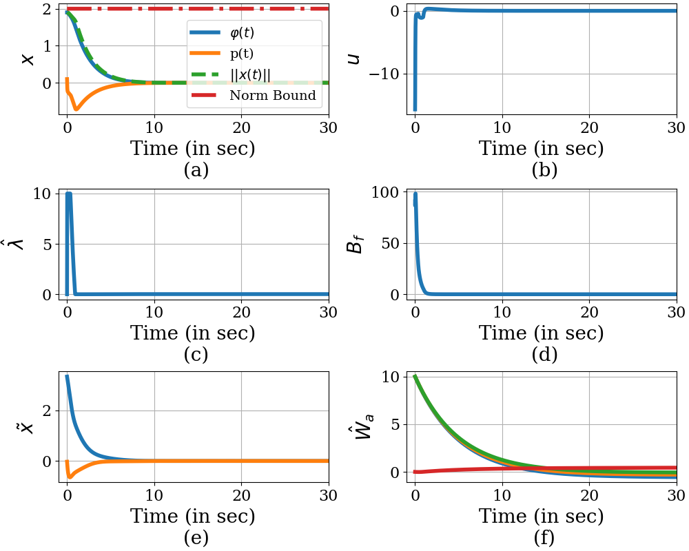
Figure 2: Relevant plots for the delta wing system (a) State trajectory along with the norm of state (b) Control effort (c) Estimated Lagrange multiplier (d) Barrier function (e) Error in the state estimation (f) Actor parameter estimate.

TABLE II: Cost comparision under different initial conditions (Lesser cost is better)

Method	Mobile robot system			Delta wing system
	$x_{0}=[4,6]^{T}$	$x_{0}=[-7.5,4.5]^{T}$	$x_{0}=[1,-9.2]^{T}$	$x_{0}=[1,0.1]^{T}$	$x_{0}=[-1,1]^{T}$	$x_{0}=[1.9,0.1]^{T}$
ACIL (ours)	107.521	157.371	176.693	13.493	4.069	11.270
Controller in [15]	111.201	158.460	173.076	14.273	4.074	15.704
ACIL (ours) with known $\theta$	91.107	136.811	161.481	4.835	4.046	12.075
Controller in [15] with known $\theta$	98.291	148.323	164.911	4.886	4.048	15.708
SGSA[1] (offline with known $\theta$)	67.892	99.282	93.444	2.338	2.270	8.205

VII-B Mobile robot in a minefield

To demonstrate the efficacy of the proposed ACIL algorithm on complex state constraints, we consider a mobile robot with single integrator dynamics $\dot{x}=u$ where $x(t),u(t)\in\mathbb{R}^{2}$. The objective of the mobile robot is to reach the origin while avoiding “mines” strewn across a “minefield”. We consider twelve mines placed randomly inside a circle of radius 10 centered at origin. The $i^{th}$ obstacle is considered to be a unit circle with center at $c_{i}\;\;\forall\;i\in\mathbb{N}_{12}$ . To incorporate this complex constraint on the state, we consider the BLF $B_{f}=B_{field}+\sum_{i=1}^{12}B_{obs_{i}}$, where $B_{field}=(\frac{100}{100-x^{T}x}-1)^{2}$ is the barrier function for the field and $B_{obs_{i}}=\frac{1}{\|x-c_{i}\|^{2}-1}$ is the barrier function for an individual obstacle. We choose $Q(x)=x^{T}x$ and $R=\mathbb{I}_{2}$ for the given optimal regulation problem. To learn an optimal control policy, we consider the basis function $\phi(x)=[x_{1}^{2},x_{1}x_{2},x_{2}^{2}]^{T}$ and the actor-critic parameters were initialized as $\hat{W}_{a}(0)=\hat{W}_{c}(0)=[2,0,2]^{T}$. The gains for the actor-critic and the Lagrangian components of the algorithm were taken to be the same values as that of the delta-wing system.

We compare the proposed method with that of [15], which is an online RL algorithm. The algorithm in [15] can be considered as the ACIL method with a constant $\hat{\lambda}$ (Technically, the constant $c_{b}$ used in [15] is related to a constant $\hat{\lambda}$ by the relation $c_{b}=R^{-1}\hat{\lambda}$). To enable a fair comparision and have equivalent control effort applied, we set $c_{b}=0.075$. We additionally compare both these methods with an offline numerical method of safe Galerkin successive approximation (SGSA) detailed in [1], which assumes the complete knowledge of the system dynamics, and generates control policies close to the optimal solution.

Figure 3 shows the visualization of the three algorithms on the mobile robot system. Figure 4 shows the (a) barrier function, (b) control effort and (c) the estimate of Lagrange multiplier. We observe that both ACIL and ACI with constant $\lambda$ apply equivalent control effort, but the peak value of the barrier function is less for the proposed ACIL algorithm. Additionally, we compare the cost inccured by each of these algorithms for both the mobile robot system and the delta-wing system in Table II. We also compare the costs for ACIL and that of [15] under the complete knowledge of the drift dynamics. We observe that in both the systems, the proposed ACIL method incurs lesser cost than that of [15]. Provided the knowledge of the system dynamics, the proposed method outperforms [15].

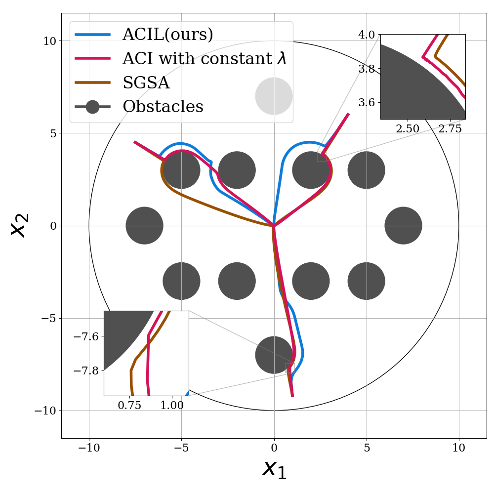
Figure 3: Visualization of the mobile robot system under different initial conditions for different RL algorithms. The blue line-plot is that of ACIL (ours), the pink line-plot is that of the algorithm detailed in [15], and the brown line-plot is that of the offline algorithm SGSA detailed in [1].

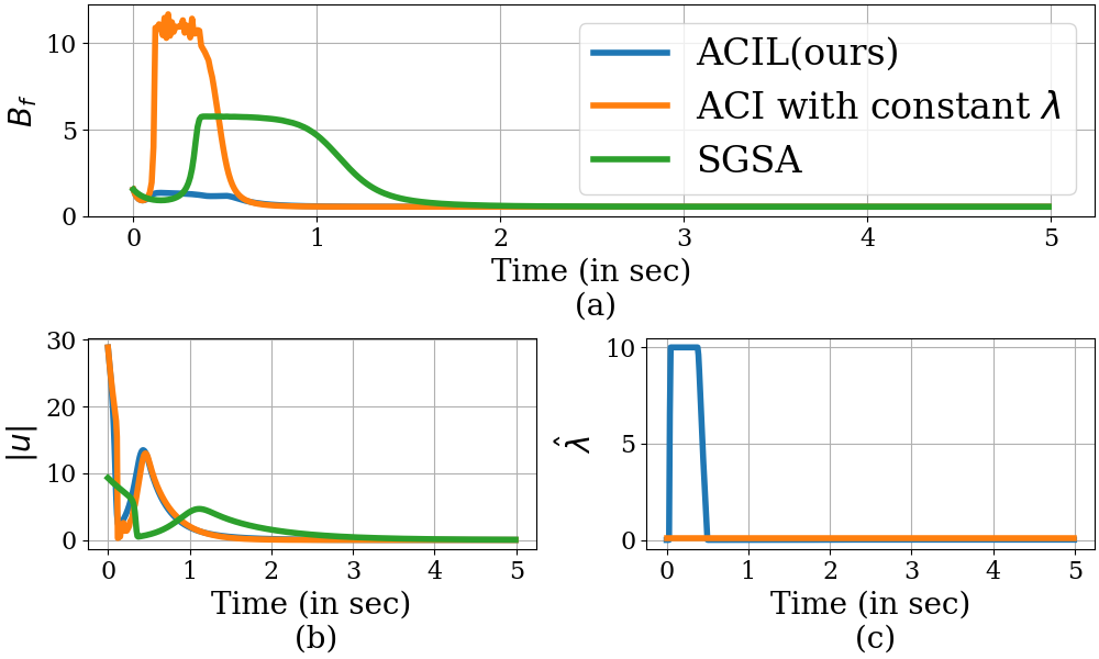
Figure 4: (a) Barrier function (b) Control effort (c) Estimated Lagrange multiplier for the mobile robot system under different algorithms. ACI with constant $\lambda$ represents the algorithm in [15] and the SGSA is the algorithm in [1].

VII-C Effect of varying the softplus gain ($k$)

We now study the effect of varying the softplus gain $k$ on the case of mobile robot system. Under different values of $k$ we tabulate the cost incurred in Table III.

TABLE III: Accrued cost under different values of softplus gain $k$ for the mobile robot system.

$k=0.02$	$k=0.1$	$k=1$	$k=5$	$k=10$
107.477	107.506	108.078	112.149	117.121

Figure 5 shows the barrier function, norm of control action, and estimate of Lagrange multiplier. We observe that as the value of $k$ increases, the cost performance deteriorates. Additionally, the control effort required increases with the increase in $k$. However, with the increase of $k$, the peak value of the BLF near the obstacles decreases.

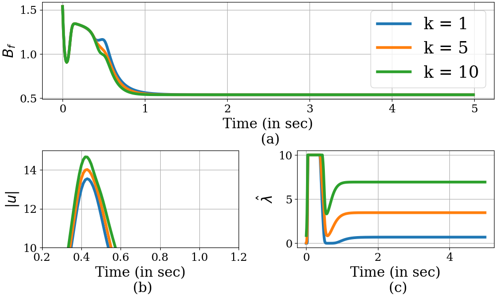
Figure 5: (a) Barrier function (b) Norm of control action (zoomed) (c) Estimate of the Lagrange multiplier, under various values of the softplus gain $k$.

VIII Conclusion

We develop an on-policy online reinforcement learning algorithm for the optimal control of a class of uncertain nonlinear systems utilizing an online estimation of Lagrange multipliers. We extend the ACI approach from [20] to learn optimal control policies in a safe fashion. We prove the safety and stability guarantees of the proposed algorithm via a Lyapunov analysis. We subsequently demonstrate the efficacy of the ACIL method on two systems in simulation. Additionally, we show that the proposed method outperforms a similar online algorithm in the literature. Future work may seek to include actuation constraints in the formulation to handle state and actuation constraints in a combined way.

Appendix A Proof of Lemma 6

Using Lemma 5, it can be shown that both $f_{\sigma}(z)$ and $f_{\sigma}^{\prime}(z)$ are monotonically increasing functions on the domain $(0,\infty)$. Additionally, we evaluate the limit $\lim_{h\rightarrow 0+}f_{\sigma}(h)=\lim_{h\rightarrow 0+}\sigma(\frac{c}{h})h=c.$ Using the properties of derivatives, we write

$$\lim_{h\rightarrow 0+}\frac{|f_{\sigma}(z)-f_{\sigma}(h)|}{|z-h|}\leq\sup_{x}|f_{\sigma}^{\prime}(x)|\;\;\forall\;z\in(0,\infty).$$ (51)

Since $f_{\sigma}^{\prime}$ is monotonically increasing, the supremum of $f_{\sigma}^{\prime}$ exists at infinity. Thus computing the said limit, we have $\frac{f_{\sigma}(z)-c}{z}\leq k\ln(2)\;\;\forall\;z\in(0,\infty),$ which on rearrangement, completes the proof.

References

- [1] Hassan Almubarak, Evangelos A Theodorou, and Nader Sadegh. Hjb based optimal safe control using control barrier functions. In 2021 60th IEEE Conference on Decision and Control (CDC), pages 6829–6834. IEEE, 2021.
- [2] Mohammed Alshiekh, Roderick Bloem, Rüdiger Ehlers, Bettina Könighofer, Scott Niekum, and Ufuk Topcu. Safe reinforcement learning via shielding. In Proceedings of the AAAI Conference on Artificial Intelligence, volume 32, 2018.
- [3] Aaron D Ames, Samuel Coogan, Magnus Egerstedt, Gennaro Notomista, Koushil Sreenath, and Paulo Tabuada. Control barrier functions: Theory and applications. In 2019 18th European control conference (ECC), pages 3420–3431. IEEE, 2019.
- [4] Aaron D Ames, Xiangru Xu, Jessy W Grizzle, and Paulo Tabuada. Control barrier function based quadratic programs for safety critical systems. IEEE Transactions on Automatic Control, 62(8):3861–3876, 2016.
- [5] Richard Bellman. Dynamic programming. Science, 153(3731):34–37, 1966.
- [6] Felix Berkenkamp, Matteo Turchetta, Angela Schoellig, and Andreas Krause. Safe model-based reinforcement learning with stability guarantees. Advances in neural information processing systems, 30, 2017.
- [7] Shubhendu Bhasin, Rushikesh Kamalapurkar, Marcus Johnson, Kyriakos G Vamvoudakis, Frank L Lewis, and Warren E Dixon. A novel actor–critic–identifier architecture for approximate optimal control of uncertain nonlinear systems. Automatica, 49(1):82–92, 2013.
- [8] Shalabh Bhatnagar, Richard S Sutton, Mohammad Ghavamzadeh, and Mark Lee. Natural actor–critic algorithms. Automatica, 45(11):2471–2482, 2009.
- [9] Franco Blanchini. Set invariance in control. Automatica, 35(11):1747–1767, 1999.
- [10] Stephen Boyd and Lieven Vandenberghe. Convex optimization. Cambridge university press, 2004.
- [11] Stephen L Campbell and Carl D Meyer. Generalized inverses of linear transformations. SIAM, 2009.
- [12] Richard Cheng, Gábor Orosz, Richard M. Murray, and Joel W. Burdick. End-to-end safe reinforcement learning through barrier functions for safety-critical continuous control tasks. 33rd AAAI Conference on Artificial Intelligence, AAAI 2019, 31st Innovative Applications of Artificial Intelligence Conference, IAAI 2019 and the 9th AAAI Symposium on Educational Advances in Artificial Intelligence, EAAI 2019, pages 3387–3395, 2019.
- [13] Max H Cohen and Calin Belta. Approximate optimal control for safety-critical systems with control barrier functions. In 2020 59th IEEE Conference on Decision and Control (CDC), pages 2062–2067. IEEE, 2020.
- [14] Max H Cohen and Calin Belta. Model-based reinforcement learning for approximate optimal control with temporal logic specifications. In Proceedings of the 24th International Conference on Hybrid Systems: Computation and Control, pages 1–11, 2021.
- [15] Max H Cohen and Calin Belta. Safe exploration in model-based reinforcement learning using control barrier functions. Automatica, 147:110684, 2023.
- [16] Jaime F Fisac, Anayo K Akametalu, Melanie N Zeilinger, Shahab Kaynama, Jeremy Gillula, and Claire J Tomlin. A general safety framework for learning-based control in uncertain robotic systems. IEEE Transactions on Automatic Control, 64(7):2737–2752, 2018.
- [17] William W Hager, Hongyan Hou, Subhashree Mohapatra, Anil V Rao, and Xiang-Sheng Wang. Convergence rate for a radau hp collocation method applied to constrained optimal control. Computational Optimization and Applications, 74(1):275–314, 2019.
- [18] William W Hager, Jun Liu, Subhashree Mohapatra, Anil V Rao, and Xiang-Sheng Wang. Convergence rate for a gauss collocation method applied to constrained optimal control. SIAM Journal on Control and Optimization, 56(2):1386–1411, 2018.
- [19] Chung-Hao Hsu and C Edward Lan. Theory of wing rock. Journal of Aircraft, 22(10):920–924, 1985.
- [20] Rushikesh Kamalapurkar, Joel A Rosenfeld, and Warren E Dixon. Efficient model-based reinforcement learning for approximate online optimal control. Automatica, 74:247–258, 2016.
- [21] Hassan K Khalil. Nonlinear systems. Prentice Hall, Upper Saddle River, 2002.
- [22] Torsten Koller, Felix Berkenkamp, Matteo Turchetta, and Andreas Krause. Learning-based model predictive control for safe exploration and reinforcement learning. Proceedings of the IEEE Conference on Decision and Control, pages 6059–6066, 2018.
- [23] Vladik Ya Kreinovich. Arbitrary nonlinearity is sufficient to represent all functions by neural networks: a theorem. Neural networks, 4(3):381–383, 1991.
- [24] Eugene Lavretsky and Kevin A Wise. Robust adaptive control. In Robust and adaptive control, pages 317–353. Springer, 2013.
- [25] Frank L Lewis, Draguna Vrabie, and Vassilis L Syrmos. Optimal control. John Wiley & Sons, third edition, 2012.
- [26] SM Nahid Mahmud, Katrine Hareland, Scott A Nivison, Zachary I Bell, and Rushikesh Kamalapurkar. A safety aware model-based reinforcement learning framework for systems with uncertainties. In 2021 American Control Conference (ACC), pages 1979–1984. IEEE, 2021.
- [27] Zahra Marvi and Bahare Kiumarsi. Safe reinforcement learning: A control barrier function optimization approach. International Journal of Robust and Nonlinear Control, 31(6):1923–1940, 2021.
- [28] Vinod Nair and Geoffrey E. Hinton. Rectified linear units improve restricted boltzmann machines. In Proceedings of the 27th International Conference on International Conference on Machine Learning, ICML’10, page 807–814, Madison, WI, USA, 2010. Omnipress.
- [29] Bo Pang and Zhong-Ping Jiang. Reinforcement learning for adaptive optimal stationary control of linear stochastic systems. IEEE Transactions on Automatic Control, 2022.
- [30] Anup Parikh, Rushikesh Kamalapurkar, and Warren E Dixon. Integral concurrent learning: Adaptive control with parameter convergence using finite excitation. International Journal of Adaptive Control and Signal Processing, 33(12):1775–1787, 2019.
- [31] Anil V Rao. A survey of numerical methods for optimal control. Advances in the Astronautical Sciences, 135(1):497–528, 2009.
- [32] Sayan Basu Roy, Shubhendu Bhasin, and Indra Narayan Kar. Combined mrac for unknown mimo lti systems with parameter convergence. IEEE Transactions on Automatic Control, 63(1):283–290, 2017.
- [33] Richard S Sutton and Andrew G Barto. Reinforcement learning: An introduction. MIT press, 2018.
- [34] Keng Peng Tee, Shuzhi Sam Ge, and Eng Hock Tay. Barrier lyapunov functions for the control of output-constrained nonlinear systems. Automatica, 45(4):918–927, 2009.
- [35] Kyriakos G Vamvoudakis. Q-learning for continuous-time linear systems: A model-free infinite horizon optimal control approach. Systems & Control Letters, 100:14–20, 2017.
- [36] Kyriakos G Vamvoudakis and Frank L Lewis. Online actor–critic algorithm to solve the continuous-time infinite horizon optimal control problem. Automatica, 46(5):878–888, 2010.
- [37] Yongliang Yang, Yixin Yin, Wei He, Kyriakos G Vamvoudakis, Hamidreza Modares, and Donald C Wunsch. Safety-aware reinforcement learning framework with an actor-critic-barrier structure. In 2019 American Control Conference (ACC), pages 2352–2358. IEEE, 2019.
- [38] Mario Zanon and Sébastien Gros. Safe reinforcement learning using robust mpc. IEEE Transactions on Automatic Control, 66(8):3638–3652, 2020.