Enhanced Meta Label Correction for Coping with Label Corruption

Abstract

Traditional methods for learning with the presence of noisy labels have successfully handled datasets with artificially injected noise but still fall short of adequately handling real-world noise. With the increasing use of meta-learning in the diverse fields of machine learning, researchers leveraged auxiliary small clean datasets to meta-correct the training labels. Nonetheless, existing meta-label correction approaches are not fully exploiting their potential. In this study, we propose an Enhanced Meta Label Correction approach abbreviated as EMLC for the learning with noisy labels (LNL) problem. We re-examine the meta-learning process and introduce faster and more accurate meta-gradient derivations. We propose a novel teacher architecture tailored explicitly to the LNL problem, equipped with novel training objectives. EMLC outperforms prior approaches and achieves state-of-the-art results in all standard benchmarks. Notably, EMLC enhances the previous art on the noisy real-world dataset Clothing1M by $1.52\%$ while requiring $\times 0.5$ the time per epoch and with much faster convergence of the meta-objective when compared to the baseline approach.

1 Introduction

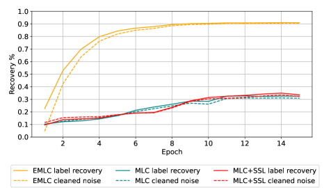
Figure 1: Comparison of the training labels recovery (solid line) and the wrong labels recovery (dashed line) over training epochs on the CIFAR-10 dataset with $90\%$ symmetric noise. EMLC (ours) is comapred to MLC [41] and to MLC [41] with self-supervised pretraining.

The remarkable success of Deep Neural Networks (DNNs) for visual classification tasks is predominantly due to the availability of massive labeled datasets. In many practical applications, obtaining the required amounts of reliable labeled data is intractable. As a result, numerous works over the past decade have sought ways to reduce the amount of labeled data required for classification tasks. Notably, semi-supervised learning exploits unlabeled data [33, 24], transfer learning exploits prior knowledge obtained from different tasks [7, 39], and self-supervised learning exploits data augmentations for label agnostic representation learning [3, 11]. Nonetheless, for many applications, the quality of the labeled data can be sacrificed for the sake of its quantity. A prominent example is the process of crawling search engines and online websites as demonstrated by [17, 32]. The crawling process is often easy to automate however results in significant amounts of label noise with complicated patterns. A fundamental problem with such data, however, is that classical learning methodologies tend to fail when significant label noise is present [36]. Therefore, designing learning frameworks that are able to cope with label corruption is a task of great importance.

While traditional methods for learning with noisy labels (LNL) are capable of handling data with immense artificial, injected noise, their ability to handle real-world noise remains highly limited. Thus, noisy labeled datasets alone limit the capability of learning from real-world noisy labeled datasets. Luckily, in many real-world applications, while obtaining large amounts of labeled data is infeasible, obtaining small amounts of labeled data is usually attainable. Thus, the paramount objective is to find methods that can incorporate both large amounts of noisy labeled data and small amounts of clean data. A natural choice is to adopt a meta-learning framework, a popular design regularly used for solving various tasks. Consequently, recent trends in LNL leverage meta-learning using auxiliary small clean datasets. Prominent examples include meta-sample weighting [26, 38], meta-robustification to artificially injected noise [16], meta-label correction [41], and meta-soft label correction [31].

In this work, we propose EMLC – an enhanced meta-label correction approach for learning from label-corrupted data. We first revise the bi-level optimization process by deriving a more accurate meta gradient used to optimize the teacher. In particular, we derive an exact form of the meta-gradient for the one-step look-ahead approximation and suggest an improved meta-gradient approximation for the multi-step look-ahead approximation. We further provide an algorithm for efficiently computing our derivations using a modern hardware accelerator. We empirically validate our derivations, demonstrating a significant improvement in convergence speed and training time. We further propose a dedicated teacher architecture that employs a feature extraction to generate initial predictions and incorporates them with the noisy label signal to generate refined soft labels for the student. Our teacher architecture is completely independent of the student, avoiding the confirmation bias problem. In addition, we propose a novel auxiliary adversarial training objective for enhancing the effectiveness of the teacher’s label correction mechanism. As demonstrated in fig. 1, our teacher proves to have a superior ability of purifying the training labels.

Our contributions can be summarized as follows:

• We derive fast and more accurate procedures for computing the meta-gradient used to optimize the teacher.

• We design a unique teacher architecture in conjunction with a novel training objective toward an improved label correction process.

• We combine these two components into a single yet effective framework termed EMLC. We demonstrate the effectiveness of EMLC on both synthetic and real-world label-corrupted standard benchmarks.

2 Related work

The LNL problem was previously addressed by various approaches. For instance, multiple works iteratively modified the labels to better align with the model’s predictions [25, 27], estimated the noise transition matrix [8], or applied a regularization [21, 37]. The common pitfall of these methods is the phenomenon that DNNs tend to develop a confirmation bias, which causes the model to the confirm the corrupted labels. To this end, Han et al. [9] proposed a two-model framework that employs a cross-model sample selection for averting the confirmation bias problem. Being remarkably successful, many follow-up works tried to build on the two-model framework by either improving the sample selection process or using semi-supervised tools to exploit the high-loss samples and leveraging label-agnostic pretraining [2, 15, 40].

Nevertheless, there is still a noticeable gap between the effectiveness of LNL methods and fully supervised training, especially on datasets with real-world noise. In numerous practical scenarios, acquiring substantial quantities of labeled data may be impractical, but obtaining a small amount of labeled data is typically achievable. This observation motivates the use of meta-learning for tackling the LNL problem. Consequently, multiple researchers have tried to exploit auxiliary small labeled datasets to apply meta-learning for LNL research.

Outside of LNL research, meta-learning has begun to appear in diverse fields in machine learning, including neural architecture search [18], hyperparameter tuning [20], few-shot learning [6] and semi-supervised learning [24]. Meta-learning often involves two types of objectives: an inner (lower-level) objective and a meta (upper-level) objective. Usually, meta-learning tasks are equipped with a large training set and a small validation set. The validation data (in many cases) is necessary for updating the meta-objective.

In the context of LNL, researchers leverage meta-learning to mitigate the effect of the label noise. In particular, [26, 38] try to weight samples to degrade the effect of noisy samples on the loss. MLNT [16] use a student–teacher paradigm and try to artificially inject random labels into the data used to train the student model. The student is encouraged to be close to the teacher model that does not observe the noisy data. Meta-label correction [41] and MSLC [31] follow the student–teacher paradigm but, unlike MLNT [16], use the teacher to produce soft training targets for the student. The soft targets are produced in such a way that when the student is trained with respect to these targets, it performs well on the clean data.

EMLC builds upon the meta-label correction framework, which, as presented in prior work [41, 31], does not appear to have fully exploited its potential. We claim that the main pitfall of current label correction frameworks is that their teacher architecture is strongly entangled to the student, resulting in a severe confirmation bias. On the contrary, EMLC is composed of a completely independent teacher, averting this problem. In addition, EMLC leverages artificial noise injection for robust training. Opposed to [16] however, we propose adversarial noise injection that we discover to be more effective for robustifying models against label noise. Another major difference is that we use the artificial noise injection to better train the teacher whereas [16] use it to train the student.

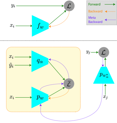
Figure 2: Classical supervised learning via empirical risk minimization (upper part). Meta-learning for generating corrected labels via clean feedback optimization (lower part). The meta-gradients are propagated through the optimization path of $p_{w}$ w.r.t. $w$. The optimized student is denoted by $p_{w^{*}_{\alpha}}$

3 Methods

In this section we discuss the distinct components of the proposed method. We start by introducing the reader to the basic setting and assumptions in LNL in subsection 3.1. In subsection 3.2, we discuss the inability of classical learning algorithms (i.e Empirical Risk Minimization - ERM) to handle heavily corrupted data and look at how to exploit meta-generated labels as an alternative to the classical learning paradigm. Accordingly, subsection 3.3 is devoted to bi-level optimization that repeatedly appears in meta-learning. In subsection 3.4, we revisit meta-gradient approximation, which is the core of performing gradient-based bi-level optimization. In addition, in subsection 3.5, we demonstrate how to compute the proposed derivations efficiently. Finally, in subsection 3.6, we elaborate on the proposed label correction architecture as well as on its training scheme.

3.1 Learning with Noisy Labels Formulation

We initiate our discussion on noisy label classification by considering a probability space $(\Omega,\mathcal{F},p)$, equipped with an instance random variable: $x:\Omega\rightarrow\mathcal{X}$, along with a label and a (possibly) corrupted label random variable: $y,\widetilde{y}:\Omega\rightarrow\mathcal{Y}$ where $\mathcal{X}\subseteq\mathbb{R}^{d},\mathcal{Y}=\{1,...,C\}$ are the instance and label space, respectively. We define the clean distribution: $\mathcal{D}=(x,y)$ and the corrupted distribution: $\widetilde{\mathcal{D}}=(x,\widetilde{y})$. The restriction on the corrupted distribution is that for each class $c\in\{1,...,C\}$, the most probable corrupted label will match the true one: $c=\operatorname*{arg\,max}_{j}p(\widetilde{y}=j|y=c)$. Given a family of parameterized predictors $\{f_{w}:\mathcal{X}\rightarrow\mathcal{Y}\}$, the high level goal is to optimize the parameters $w$ to minimize the true expected risk: $\mathcal{R}(f)=\mathbb{E}_{(x,y)}[\ell(f_{w}(x),y)]$ for some loss function $\ell:\mathcal{Y}\times\mathcal{Y}\rightarrow\mathbb{R}^{+}$ by accessing mostly $\widetilde{\mathcal{D}}$. In practice, $\widetilde{\mathcal{D}}$ is most likely inaccessible and rather we are given i.i.d. samples of it $\{(x_{i},\widetilde{y}_{i})\}_{i=1}^{n}$. In the setting of interest, we are also supplied with a small set of clean i.i.d. samples $\{(x_{j},y_{j})\}_{j=1}^{m}$ where $m\ll n$.

3.2 From ERM to Meta-Learning

According to the ERM principle in supervised learning, $f_{w}$ should be optimized by considering the empirical risk:

$$w^{*}=\operatorname*{arg\,min}_{w}\frac{1}{n}\sum_{i=1}^{n}\ell(f_{w}(x_{i}),y_{i})$$ (1)

To make optimization feasible, $\ell$ is chosen to be a differentiable function. In particular, if we generalize $f_{w}$ to model a probability distribution, $p_{w}(y|x)$, the cross-entropy loss [4] is most commonly used:

$$w^{*}=\operatorname*{arg\,min}_{w}\frac{1}{n}\sum_{i=1}^{n}CE(y_{i},p_{w}(y|x_{i}))$$ (2)

In our case, the labels $\widetilde{y}_{i}$ are possibly corrupted. Therefore, applying the ERM principle would give rise to noisy label memorization (due to the universal approximation theorem) leading to a severe degradation in the obtained predictor’s performance [19, 36]. This problem is addressed by replacing $y_{i}$ with a label correction architecture $q_{\alpha}(y|x_{i},\widetilde{y}_{i})$, which will produce corrected (soft) labels for training $p_{w}$. For the ease of reading, from this point on, we refer to $p_{w}$ as the student architecture and $q_{\alpha}$ as the teacher architecture. Recall that the real goal is to optimize the student to minimize the true expected error. Hence, given a small set of clean samples, the teacher should produce soft labels in a way that would cause the optimized student to have small empirical risk on the clean set, as demonstrated in fig. 2. Therefore, the objective may be formalized as the following bi-level optimization problem:

$$\min_{\alpha}\mathcal{L}(w^{*}(\alpha))$$ (3)

$$s.t\text{ }w^{*}=\operatorname*{arg\,min}_{w}\widetilde{\mathcal{L}}(w,\alpha)$$ (4)

where:

$$\mathcal{L}(w^{*}(\alpha))=\frac{1}{m}\sum_{j=1}^{m}CE(y_{j},p_{w^{*}(\alpha)}(y|x_{j}))$$ (5)

$$\widetilde{\mathcal{L}}(w,\alpha)=\frac{1}{n}\sum_{i=1}^{n}CE(q_{\alpha}(y|x_{i},\widetilde{y}_{i}),p_{w}(y|x_{i}))$$ (6)

Note that under relatively mild conditions, $w^{*}$ can be written (locally) as a function of $\alpha$. This can be observed from stationary conditions applied to eq. 4: $\nabla_{w}\widetilde{\mathcal{L}}(w,\alpha)=0$ and applying the implicit function theorem.

3.3 Bi-Level Optimization

Bi-level optimization problems appear in diverse sub-fields in machine learning and in meta-learning in particular [18, 20, 6, 24]. Such problems are composed of an outer level optimization problem that is usually constrained by another inner level problem. We relate to the upper level problem parameters as the meta-parameters and to the parameters in the lower level as the main parameters. The fact that each meta-parameter value defines a new lower level problem makes applying gradient-based optimization methods to such situations particularly difficult due to the iteration complexity. A solution to this problem is to approximate $w^{*}$ with $k$-step look-ahead SGD, optimizing both the main and meta- parameters simultaneously. The joint optimization process can be summarized in algorithm 1.

Algorithm 1 Bi-Level Optimization via $k$-step SGD Look-ahead Approximation

1:Clean and noisy datasets $\mathcal{D},\widetilde{\mathcal{D}}$, number of training steps $T$, initial parameters $w^{(0)},\alpha^{(0)}$, learning rates $\eta_{w},\eta_{\alpha}$.

2:Optimized parameters $w^{(T)},\alpha^{(T)}$.

3:for $t=0$ ,…, $T-1$ do

4:     // Sample clean and noisy batches from the datasets

5:     $\mathcal{B},\widetilde{\mathcal{B}}\leftarrow Sample(\mathcal{D}),Sample(\widetilde{\mathcal{D}})$

6:     // Update $w$ by descending $\widetilde{\mathcal{L}}(w,\alpha)$ w.r.t $w$

7:     $w^{(t+1)}\leftarrow w^{(t)}-\eta_{w}\nabla_{w}\widetilde{\mathcal{L}}(w,\alpha^{(t)})\bigg{\rvert}_{w=w^{(t)}}$

8:     if $t\ \mathrm{mod}\ k=k-1$ then

9:         // Unroll $w^{(t+1)}(\alpha)$ to compute the meta gradient

10:         $g_{\alpha}=\text{{META\_GRAD}}(\mathcal{L}(w^{(t+1)}),\alpha)$

11:         // Update $\alpha$ by descending $\mathcal{L}(w^{(t+1)}(\alpha))$ w.r.t $\alpha$

12:         $\alpha^{(t+1)}\leftarrow\alpha^{(t)}-\eta_{\alpha}g_{\alpha}$

13:     else

14:         $\alpha^{(t+1)}\leftarrow\alpha^{(t)}$

15:     end if

16:end for

During training, the higher order dependencies of $w$ on $\alpha$ are neglected, thereby allowing the meta-gradient to be computed, as we discuss in the next section.

3.4 Revisiting the Meta-Gradient Approximation

As opposed to Meta-Label Correction [41], we propose better approximations for both the single and multi-step meta-gradients when updating the teacher. In the next section, we establish an efficient method for carrying out the meta-gradient computation.

We explicitly differentiate between the cases $k=1$ and $k>1$. We begin by deriving the one-step approximation meta-gradient.

Proposition 1.

(One-Step Meta-Gradient) Let $g_{w}:=\nabla_{w}\mathcal{L}(w^{(t+1)})$ where $w^{(t+1)}$ are the student’s new parameters obtained when last updated. Let $H_{w\alpha}^{(t)}:=\nabla_{w\alpha}\widetilde{\mathcal{L}}(w^{(t)},\alpha^{(t)})$ where $w^{(t)}$ are the student’s original parameters (before its update). Let $\alpha^{(t)}$ be the teacher’s parameters before its update. Then, the one-step meta-gradient at time $t$ denoted by $\nabla_{\alpha}^{(t)}$ is given by:

$$[\nabla_{\alpha}^{(t)}]^{T}=-\eta_{w}g_{w}^{T}H_{w\alpha}^{(t)}$$ (7)

The proof of proposition 1 is given in subsection A.1. We proceed by considering the case of $k>1$. In this case, we do not compute the exact meta-gradient. Instead, we approximate it.

Proposition 2.

($k$-Step Meta-Gradient Approximation with Exponential Moving Average of Mixed Hessians) Assume that $t\ \mathrm{mod}\ k=k-1$ and let $g_{w}:=\nabla_{w}\mathcal{L}(w^{(t+1)})$ where $w^{(t+1)}$ is the student’s new parameters obtained when last updated. Consider the mixed Hessians in the last $k$ steps: $H_{w\alpha}^{(\tau)}:=\nabla_{w\alpha}\widetilde{\mathcal{L}}(w^{(\tau)},\alpha^{(\tau)})$ where $t-k+1\leq\tau\leq t$. Let $\alpha^{(t)}=\alpha^{(t-1)}=...=\alpha^{(t-k+1)}$ be the teacher’s parameters before its update. Then, the $k$-step meta-gradient denoted by $\nabla_{\alpha}$ can be approximated by:

$$[\nabla_{\alpha}^{(t)}]^{T}\approx-\eta_{w}g_{w}^{T}\sum_{\tau=t-k+1}^{t}\gamma_{w}^{t-\tau}H_{w\alpha}^{(\tau)}$$ (8)

where $\gamma_{w}=1-\eta_{w}$.

The proof of proposition 2 is given in subsection A.2.

3.5 Computational Efficiency of the Meta-Gradient

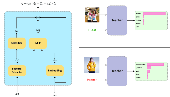
Figure 3: The proposed teacher architecture (left) and typical teacher’s output distributions when fed with clean/noisy sample (right). In our architecture, the sample is initially fed to a feature extractor to obtain a representation $h_{i}$ and then to a classifier to obtain an initial prediction $\hat{y}_{i}$. The (possibly) noisy label is then fed to an embedding layer to obtain a label embedding $z_{i}$. Both of the embeddings are then concatenated and are fed to an MLP which produces a weight $w_{i}\in(0,1)$. Finally, $w_{i}$ is used to gate the initial prediction and the noisy label to produce the final prediction.

Calculating the one-step meta-gradient as in proposition 1 or the multi-step meta-gradient as in proposition 2 in a straightforward manner is inefficient, as it requires computing higher-order derivatives of large DNNs. In this section, we provide a few workarounds that allow us to carry out the computations efficiently. Our first observation is that the sample-wise mixed Hessian can be expressed as a product of two first-order Jacobians. Formally:

Proposition 3.

Let us consider the sample-wise lower loss: $\widetilde{\ell}_{i}(w,\alpha):=CE(q_{\alpha}(y|x_{i},\widetilde{y}_{i}),p_{w}(y|x_{i}))$. Recall from eq. 6 that $\widetilde{\mathcal{L}}(w,\alpha)=\frac{1}{n}\sum_{i=1}^{n}\widetilde{\ell}_{i}(w,\alpha)$. Denote by $J_{w}(i):=J_{w}(\log(p_{w}(y|x_{i})))$ and by $J_{\alpha}(i):=J_{\alpha}(q_{\alpha}(y|x_{i},\widetilde{y}_{i}))$. We claim that:

$$\nabla_{w\alpha}\widetilde{\ell}_{i}(w,\alpha)=-[J_{w}(i)]^{T}[J_{\alpha}(i)]$$ (9)

The proof of proposition 3 is given in subsection A.3.

Corollary 3.1.

Using proposition 1, the one-step meta-gradient can be expressed as:

$$[\nabla_{\alpha}^{(t)}]^{T}=\frac{\eta_{w}}{n}\sum_{i=1}^{n}g_{w}^{T}[J_{w^{(t)}}(i)]^{T}[J_{\alpha^{(t)}}(i)]$$ (10)

Using proposition 2 the k-step meta-gradient approximation can be expressed as:

$$[\nabla_{\alpha}^{(t)}]^{T}=\frac{\eta_{w}}{n}\sum_{i=1}^{n}\sum_{\tau=t-k+1}^{t}\gamma_{w}^{t-\tau}g_{w}^{T}[J_{w^{(\tau)}}(i)]^{T}[J_{\alpha^{(t)}}(i)]$$ (11)

Dataset	CIFAR-10					CIFAR-100
Method	20%	50%	80%	90%	Asym. 40%	20%	50%	80%	90%
Cross-Entropy	86.8	79.4	62.9	42.7	83.2	62.0	46.7	19.9	10.1
MW-Net [26]	89.76	–	56.56	–	88.69	66.73	–	19.04	–
MLNT [16]	92.9	88.8	76.1	58.3	88.6	67.7	58.0	40.1	14.3
MLC [41]	92.6	88.1	77.4	67.9	–	66.5	52.4	18.9	14.2
MSLC [31]	93.4	89.9	69.8	56.1	91.6	72.5	65.4	24.3	16.7
FasTEN [14]	91.94	90.07	86.78	79.52	90.43	68.75	63.82	55.22	–
EMLC ($k=1$)	91.8  $\pm$ 0.51	91.16  $\pm$ 0.25	90.95  $\pm$ 0.24	90.71  $\pm$ 0.07	91.81  $\pm$ 0.05	72.48  $\pm$ 0.44	67.08  $\pm$ 0.35	60.37  $\pm$ 0.31	54.04  $\pm$ 0.57
EMLC ($k=5$)	93.53  $\pm$ 0.21	92.63  $\pm$ 0.05	89.89  $\pm$ 0.07	89.57  $\pm$ 0.30	91.82  $\pm$ 0.19	73.05  $\pm$ 0.20	68.61  $\pm$ 0.34	60.51  $\pm$ 0.19	52.49  $\pm$ 0.18

Table 1: Comparison with state-of-the-art methods in test accuracy (%) on CIFAR-10 and CIFAR-100 datsets corrupted with multiple levels and types of noise. The reported standard deviations are based on $5$ runs using different seeds for each setting.

corollary 3.1 can be exploited to compute the meta-gradient efficiently as demonstrated in algorithm 2.

Algorithm 2 Fast and Precise Meta Gradients (FPMG)

1:Student weights obtained from the inner problem iterations $w^{(t-k+1)},...,w^{(t+1)}$, last teacher weights $\alpha^{(t)}$.

2:Meta-gradient for the current iteration $\nabla_{\alpha}^{(t)}$.

3:$g_{w}\leftarrow\nabla_{w}\mathcal{L}(w^{(t+1)})$ // Student feedback gradient

4:$\nabla_{\alpha}^{(t)},d_{w}\leftarrow 0_{\alpha},1$

5:for $\tau=t,...,t-k+1$ do

6:     for $i\in\widetilde{\mathcal{B}}$ do

7:         // Compute JVP using forward mode AD

8:         $jvp_{i}\leftarrow[J_{w^{(t)}}(i)]g_{w}$

9:         // Compute VJP using backward mode AD

10:         $res_{i}\leftarrow(jvp_{i})^{T}[J_{\alpha^{(t)}}(i)]$

11:     end for

12:     // Accumulate the contribution of $\tau$ to $\nabla_{\alpha}^{(t)}$

13:     $\nabla_{\alpha}^{(t)}\leftarrow\nabla_{\alpha}^{(t)}+d_{w}\frac{\eta_{w}}{n}\sum_{i=1}^{n}res_{i}$

14:     $d_{w}\leftarrow(1-\eta_{w})d_{w}$ // Update discount factor

15:end for

In terms of computation, the FPMG algorithm can be easily batchified and hence takes roughly only three times the computation required for a single backward mode AD used in a simple lower level update. In terms of memory (in addition to the original and updated student parameters), only the intermediate variables that accumulate for a one-student gradient and an $n\times C$ matrix for storing the JVPs for all the samples, must be stored, which is very efficient.

Since the computation grows linearly with the number of batches, the only bottleneck in the approach is the memory required to store all the $k+1$ versions of the student’s parameters obtained in its optimization process. This is a standard snag in such bi-level optimization problems [6, 42]. A summary of the differences of FPMG from MLC’s [41] meta gradient computation is given in appendix B.

3.6 Teacher Architecture and Optimization

Recall that the key to applying meta-learning to the LNL problem lies in the teacher architecture. The teacher $q_{\alpha}(y|x_{i},\widetilde{y}_{i})$ aims to correct the labels of (possibly) corrupted sample–label pairs, given the sample and its corresponding (possibly) corrupted label. Thus, it is important to design an appropriate teacher architecture. We propose a teacher architecture which is especially tailored for correcting corrupted labels. In contrast to MLC [41] and MSLC [31], our teacher architecture possesses its own feature extractor and a classifier to produce its own predictions. As a result, the proposed label correction procedure is completely disentangled from the student. This structure decreases noisy label memorization and confirmation bias. In addition, the proposed architecture carefully takes advantage of the noisy label signal. The noisy label is used to extract label embedding, which is then combined with the image embedding and fed to an MLP with a single output neuron. The MLP learns to gate the teacher’s predictions and the input noisy label so that when the input label is not actually corrupted, the input label signal would be preferred. Our proposed teacher architecture is summarized in fig. 3. In addition to the meta-learning optimization objective, the unique structure of the proposed architecture enables us to further leverage the extra clean data to design additional supervised learning objectives for training the teacher. We first notice that both the feature extractor and the classifier can be trained by considering simple supervised cross entropy loss on the clean training data. Followed by the findings in [22], we apply AutoAugment data augmentation [5] on the extra clean data. Nonetheless, the label embedding layer and the label-retaining MLP predictor are omitted from this loss. To this end, we propose to artificially inject noise into a portion of the clean training data and encourage the MLP to predict whether the input label is clean or corrupted. In practice, we corrupt half of each clean training batch and use binary cross-entropy loss at the end of the MLP. We propose two corruption strategies; in the random corruption strategy, we sample uniformly i.i.d. random labels and assign them to half of the batch; in the adversarial corruption strategy, we corrupt an image’s label with the strongest incorrect prediction obtained by the teacher’s classifier. We hypothesize that the adversarial corruption strategy would cause the MLP to identify clean labels when the teacher’s predictions are uncertain. The final teacher training objective can be summarized as follows:

$$\mathcal{L}(\alpha)=\mathcal{L}_{CE}(\alpha)+\mathcal{L}_{BCE}(\alpha)+\mathcal{L}_{META}(w^{*}(\alpha))$$ (12)

4 Experiments

In this section, we extensively verify the empirical effectiveness of EMLC, both qualitatively and quantitatively.

In subsections 4.1 and 4.2 we verify the empirical effectiveness of EMLC on the three major benchmark datasets used in the literature [26, 41, 16, 14, 31] about meta-learning for LNL. We inject synthetic random noise at multiple levels and of assorted types into the CIFAR-10 and CIFAR-100 datasets [13], which are correctly labeled datasets. On the other hand, the Clothing1M dataset [32] is a massive dataset collected from the internet, containing many mislabeled examples. In all our experiments on the benchmark datasets we validate EMLC with both the single-step look-ahead optimization strategy and the multi-step optimization strategy.

In subsection 4.3 we discuss the efficiency of the proposed meta-learning procedures used in EMLC in terms of computation time and speed of convergence.

Method	Extra Data	Test accuracy
Cross-entropy	✗	69.21
Joint-Optim [28]	✗	72.16
P-correction [35]	✗	73.49
C2D [40]	✗	74.30
DivideMix [15]	✗	74.76
ELR+ [19]	✗	74.81
AugDesc [22]	✗	75.11
SANM [29]	✗	75.63
Meta Cleaner [38]	✓	72.50
Meta-Learning [16]	✓	73.47
MW-Net [26]	✓	73.72
FaMUS [34]	✓	74.40
MLC [41]	✓	75.78
MSLG [1]	✓	76.02
Self Learning [10]	✓	76.44
FasTEN [14]	✓	77.83
EMLC ($k=1$)	✓	79.35
EMLC ($k=5$)	✓	78.16

Table 2: Comparison with state-of-the-art methods in test accuracy (%) on Clothing1M. The methods in the lower part of the table use extra clean data, while the methods in the upper part do not (above an below the dividing line).

In subsection C.1 we perform ablation studies on the distinct components of EMLC and on the number of look-ahead steps.

4.1 CIFAR-10/100

CIFAR-10 is a $10$ class dataset consisting of $50$k training and $10$k testing RGB tiny images. Likewise, CIFAR-100 is a $100$ class dataset with images of the same dimensionality and the same total amount of training and testing images.

To evaluate the effectiveness of the EMLC framework, we follow previous works on meta-learning for LNL [26, 16, 14, 31] and adopt the standard protocol for validating our framework. For the small clean dataset, $1,000$ samples are randomly selected and separated from the training data. The small clean dataset is balanced, yielding $100$ instances from each category in the CIFAR-10 dataset and $10$ samples from each category in the CIFAR-100 dataset. The rest of the training data is designated as the ”large” noisy dataset and is injected with artificial label noise.

Two distinct settings for the noise injection are used: Symmetric and Asymmetric noise. As these are standard in LNL research, we refer the reader to subsection E.1 for more details on these settings.

Following prior work, in the CIFAR-10 experiments we use ResNet-34 architecture [12] whereas in the CIFAR-100 experiments we use ResNet50 architecture. In both experiments we initialize the model using SimCLR [3] self-supervised pretraining, following [40]. We note that owing to self-supervised pretraining, only $15$ epochs are needed for obtaining optimal results. We report our results on the CIFAR datasets with $\{20\%,50\%,80\%,90\%\}$ symmetric noise and $40\%$ asymmetric noise in CIFAR-10. We treat the clean data as a validation set, and report the results using the student model when its validation score is the highest. We compare our results with previous methods in table 1.

EMLC proves to be very effective, obtaining state-of-the-art results in all the experiments. Notably, EMLC superbly surpasses prior works when facing high noise levels, maintaining an accuracy of more than $90\%$ in CIFAR-10 and more than $50\%$ in CIFAR-100 at a $90\%$ noise rate. Furthermore, EMLC shows an impressive improvement over the state-of-the-art methods of $2.16\%$ on CIFAR-10 and $3.58\%$ on CIFAR-100 in medium-level $50\%$ noise setting. We observe that although both the one-step and multi-step strategies are superior to prior methods, the multi-step strategy worked the best. Regarding the number of steps chosen for the multi-step strategy, in our experiments we found that $k=5$ was optimal. In subsection C.1 we show that $k=5$ is indeed optimal for the $50\%$ noise rate in CIFAR-100.

4.2 Clothing1M

Clothing1M is a large-scale clothing dataset obtained by crawling images from several online shopping websites. The dataset consists of $14$ classes. The dataset contains more than a million noisy labeled samples as well as a small set (around $50K$) of clean samples and small validation and testing datasets. We follow prior works on LNL [15, 22, 16] and use ResNet-50 architecture [12] pretrained on ImageNet. We train both architectures for $5$ epochs, using both the single-step and multi-step look-ahead strategies. Additional experimental details can be found in subsection E.2. As in the CIFAR experiments, we report the results using the student model with the highest validation score. We compare our results with previous approaches in table 2. As can be observed, our method reaches a clear-cut result on the challenging Clothing1M dataset that surpasses the state-of-the-art methods by $1.52\%$. In addition, the results show a significant improvement of over $3.5\%$ to MLC [41]. In contrast to our CIFAR experiments, in the Clothing1M experiment, the one-step meta-gradient proved to be better than the multi-step meta-gradient, showing the essence of both strategies. Qualitatively, we visually compare the validation set representations of the trained student model of EMLC and MLC[41] using a t-SNE [30] plot in fig. 4. As can be observed, EMLC manages to keep the same categories clustered whereas MLC [41] fails to do so on multiple categories.

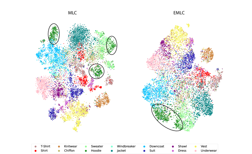
Figure 4: Comparison of the tSNE plot of the validation set embeddings obtained by the student when trained on Clothing1M.

4.3 Meta-Learning

We now discuss the empirical effectiveness of our meta-gradient approximation and computation, demonstrated on the Clothing1M dataset.

In terms of speed of convergence, we compare the convergence, in MLC [41] and EMLC, of the student’s meta-evaluation loss . Recall that the meta-learning objective is to reduce this loss. The loss dynamics are presented in fig. 5. Note that the meta-regularization loss of EMLC converges in the first two epochs for both $k=1$ and $k=5$. In contrast, MLC’s [41] regularization loss has yet to converge at this point and has a much noisier optimization process. In addition, it can be observed that our method (for both $k=1$ and $k=5$) has a lower clean feedback loss compared to MLC. In the Clothing1M experiment, however, the single-step optimization process dominates the multi-step optimization process in terms of the final loss value, which correlates with the final accuracy.

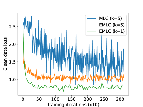
Figure 5: The meta-objective value for the first two epochs. The horizontal axis indicates the training iterations.

In terms of computation, we compare the time required by EMLC and MLC [41] to complete a single epoch (in hours) using a single A6000 GPU. We find out that MLC [41] takes $7.241$ hours whereas EMLC takes $3.67$ hours with $k=1$ and $3.467$ hours with $k=5$. Our approach is twice as fast as MLC [41] despite using a noticeably larger teacher model. This indicates that our meta-gradient computation is extremely efficient, and allows the deployment of our method to large scale datasets.

5 Discussion

In this paper we proposed EMLC – an enhanced meta-label correction framework for the learning with noisy labels problem. We proposed new meta-gradient approximations for both the single and multi-step optimization strategies and showed that they can be computed very efficiently. We further offered a teacher architecture that is better aimed to handle label noise. We present a novel adversarial noise injection mechanism and train the teacher architecture using both regular supervision and meta-supervision.

EMLC surpasses previous methods on benchmark datasets, demonstrating an extraordinary performance improvement of $1.52\%$ on the real noise dataset Clothing1M.

Our proposed meta-learning strategies are accurate and fast in terms of computation and speed of convergence. As such, despite their application to LNL, we persume that our proposed meta learning strategies can be exploited in other distinct meta-learning problems.

Appendix A Proofs

A.1 Proof of Proposition 1

Proof.

The student’s update rule parameterized by $\alpha$ is given by:

$$w^{(t+1)}(\alpha)=w^{(t)}-\eta_{w}\nabla_{w}\widetilde{\mathcal{L}}(w,\alpha)\bigg{\rvert}_{w=w^{(t)}}$$ (13)

Differentiating eq. 13 w.r.t $\alpha$ yields:

$$\frac{dw^{(t+1)}}{d\alpha}\bigg{\rvert}_{\alpha=\alpha^{(t)}}=-\eta_{w}\nabla_{w\alpha}\widetilde{\mathcal{L}}(w,\alpha)\bigg{\rvert}_{(w^{(t)},\alpha^{(t)})}$$ (14)

We now can compute the meta-gradient explicitly using the chain rule as follows:

$$\frac{d\mathcal{L}}{d\alpha}\bigg{\rvert}_{\alpha=\alpha^{(t)}}=\frac{d\mathcal{L}}{dw^{(t+1)}}\bigg{\rvert}_{w^{(t+1)}=w^{(t+1)}}\cdot\frac{dw^{(t+1)}}{d\alpha}\bigg{\rvert}_{\alpha=\alpha^{(t)}}$$ (15)

Where $w^{(t+1)}$ is obtained from the updated student.

Substituting eq. 14 we obtain the desired result. ∎

A.2 Proof of Proposition 2

Proof.

In the case $k>1$, we have:

$$w^{(t-k+2)}(\alpha)=w^{(t-k+1)}-\eta_{w}\nabla_{w}\widetilde{\mathcal{L}}(w^{(t-k+1)},\alpha)$$ (16)

Recall that we neglect the dependency of $w^{(t-k+1)}$ on $\alpha$. In addition, for all $t-k+2\leq\tau\leq t$:

$$w^{(\tau+1)}(\alpha)=w^{(\tau)}(\alpha)-\eta_{w}\nabla_{w}\widetilde{\mathcal{L}}(w^{(\tau)}(\alpha),\alpha)$$ (17)

Recall also that:

$$\forall t-k+1\leq\tau\leq t:\alpha^{(\tau)}=\alpha^{(t)}$$ (18)

We denote:

$$H_{w\alpha}^{(\tau)}:=\nabla_{w\alpha}\widetilde{\mathcal{L}}(w^{(\tau)},\alpha^{(\tau)})$$ (19)

$$H_{ww}^{(\tau)}:=\nabla_{ww}\widetilde{\mathcal{L}}(w^{(\tau)},\alpha^{(\tau)})$$ (20)

deriving eq. 17 w.r.t $\alpha$ (considering the derivative at $\alpha=\alpha^{(t)}$), using the chain rule again and substituting eq. 18 yields:

$$\frac{dw^{(\tau+1)}}{d\alpha}=\frac{dw^{(\tau)}}{d\alpha}-\eta_{w}[H_{ww}^{(\tau)}\cdot\frac{dw^{(\tau)}}{d\alpha}+H_{w\alpha}^{(\tau)}]$$ (21)

We rewrite the above equation as:

$$\frac{dw^{(\tau+1)}}{d\alpha}=[I-\eta_{w}H_{ww}^{(\tau)}]\cdot\frac{dw^{(\tau)}}{d\alpha}-\eta_{w}H_{w\alpha}^{(t)}$$ (22)

If we now approximate $H_{ww}^{(\tau)}\approx I$ we get:

$$\frac{dw^{(\tau+1)}}{d\alpha}=(1-\eta_{w})\frac{dw^{(\tau)}}{d\alpha}-\eta_{w}H_{w\alpha}^{(\tau)}$$ (23)

By setting $\gamma_{w}=1-\eta_{w}$, opening up the recursion formula and using eq. 16 at the end of the recursion, we get the desired result.

∎

A.3 Proof of Proposition 3

Proof.

This follows from the definition of cross-entropy and simple differentiation rules. Indeed,

$$\widetilde{\ell}_{i}(w,\alpha)=CE(q_{\alpha}(y|x_{i},\widetilde{y}_{i}),p_{w}(y|x_{i}))=$$ (24)

$$-\sum_{c=1}^{C}(q_{\alpha}(y=c|x_{i},\widetilde{y}_{i})\cdot\log(p_{w}(y=c|x_{i}))))=$$ (25)

$$-\left\langle q_{\alpha}(y|x_{i},\widetilde{y}_{i}),\log p_{w}(y|x_{i}))\right\rangle$$ (26)

Now, for two general differential functions $f(w):\mathbb{R}^{W}\rightarrow\mathbb{R}^{C}$, and $g(\alpha):\mathbb{R}^{A}\rightarrow\mathbb{R}^{C}$ consider $h(w,\alpha)=\left\langle f(w),g(\alpha)\right\rangle$. Then:

$$\nabla_{w}h(w,\alpha)=\nabla_{w}\left\langle f(w),g(\alpha)\right\rangle=(g(\alpha))^{T}J_{w}(f)$$ (27)

Differentiating both sides of the equation w.r.t $\alpha$ yields:

$$\nabla_{w\alpha}h(w,\alpha)=\frac{d\nabla_{w}h}{dg}\cdot\frac{dg}{d\alpha}=[J_{w}(f)]^{T}[J_{\alpha}(g)]$$ (28)

And hence $\nabla_{w\alpha}h(w,\alpha)$ exists and equals to $[J_{w}(f)]^{T}[J_{\alpha}(g)]$. Substituting $f,g$ from eq. 26 in the above equation yields the desired result. ∎

Appendix B Comparison of the Meta Gradient Computation

We compare the differences of our FPMG algorithm and MLC [41] in terms of the quality and efficiency of the meta-gradient computation in table 3. Prominently, FPMG avoids computing second order derivatives which yield a large memory and computation overhead.

Criterion	FPMG	MLC
Exact GD recursion	✓	✗
Exact mixed Hessian $H_{w\alpha}$	✓	✓
Avoids second-order derivative	✓	✗
Approximation of $H_{ww}$	$H_{ww}\approx I$	$H_{ww}\approx I$

Table 3: Comparison of FPMG and MLC [41] regarding the meta-gradient quality and efficiency of the computation.

Appendix C Additional Experiments

C.1 Ablation studies

We perform an ablation study on the different components of our method. Each setting is validated on the Clothing1M dataset. The results are summarized in table 4.

As can be observed from table 4, our approach possesses a very strong baseline. Each of our proposed components incrementally improves the effectiveness, as expected. Notably, it can be observed that the meta-regularization and the artificial corruption were crucial for the success of our method.

Regarding the number of look-ahead steps, we perform two ablative experiments. Following the finding that the multi-step strategy outclassed the single-step strategy in some of the CIFAR experiments, we perform an ablation study on the number of steps in the multi-step strategy on the CIFAR-100 dataset with $50\%$ symmetric noise and a fixed seed. As can be observed from the results in fig. 6, $k=5$ arbitrated to be the best. In addition, due to the importance of the Clothing1M dataset, we perform an additional ablation study to demonstrate the robustness of our method to varying number of look-ahead steps on a real-world dataset, as presented in fig. 7.

Meta Regularization	Corruption Strategy	Strong Augmentations	Accuracy
✗	✗	✗	74.35
✓	✗	✗	77.52
✓	Rand.	✗	78.51
✓	Adv.	✗	78.60
✓	Adv.	✓	79.35

Table 4: Ablation study on the distinct components of EMLC. We validate the effectiveness of each combination by considering test accuracy (%) on the Clothing1M dataset. We verify the effectiveness of the meta-learning regularization, the effectiveness of the proposed proactive noise injection and the benefit of applying AutoAugment to the labeled data. The corruption strategy values might be either none (✗– in which case, the $BCE$ loss is omitted), random (rand.) or adversarial (adv.).

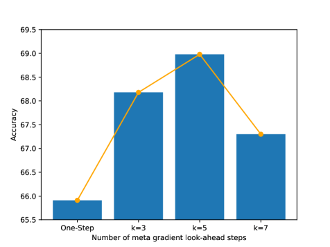
Figure 6: Ablation study on the number of look-ahead steps, measuring the effectiveness on the CIFAR-100 dataset with $50\%$ symmetric noise.

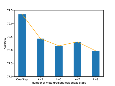
Figure 7: Ablation study on the number of look-ahead steps, measuring the effectiveness on the Clothing1M dataset.

C.2 Teacher’s Label Recovery

To further verify the teacher’s ability to cleanse the training labels, we compare the teacher’s label recovery rate (total and wrongly annotated samples) on the CIFAR-10 dataset with different noise levels of EMLC against MLC [41] and MLC with self-supervised pretraining in fig. 8.

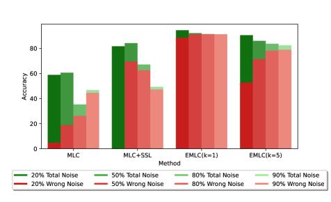
Figure 8: Comparison of the teacher’s label recovery rate (total and wrongly annotated samples) on the CIFAR-10 dataset with different noise levels.

Appendix D A probabilistic interpretation of the teacher

The goal of the teacher is to model the conditional distribution of the true label $y$ given the sample $x$ and its noisy label $\tilde{y}$, namely $p(y|x,\tilde{y})$.

The above conditional distribution can be decomposed as follows:

$$p(y|x,\tilde{y})=$$ (29)

$$w\cdot p(y|x,\tilde{y},\mathcal{A})+(1-w)\cdot p(y|x,\tilde{y},\mathcal{A}^{c})=$$ (30)

$$w\cdot\delta_{\tilde{y}y}+(1-w)\cdot p(y|x,\tilde{y},\mathcal{A}^{c})$$ (31)

where $\mathcal{A}$ is the event of $y=\tilde{y}$ and $w:=p(\mathcal{A}|x,\tilde{y})$.

In our teacher architecture, we model $w$ directly. However, we approximate $p(y|x,\tilde{y},\mathcal{A}^{c})\approx p(y|x,\mathcal{A}^{c})\approx p(y|x)$ and model $p(y|x)$ instead. In the first approximation, we throw away the conditioning on $\tilde{y}$, intuitively ignoring the cases in which $y|x$ is dependent of $\tilde{y}$ whenever the label is corrupted. While the second approximation is technically unnecessary (as $p(y|x,\mathcal{A}^{c})$ can be easily modeled by masking the SoftMax layer), we found out that the latter modeling was better in practice since it effectively enhances the weight of hard clean samples.

Appendix E Further Details of the Experimental Setting

E.1 Symmetric and Asymmetric Artificial Noise

In the Symmetric noise setting, a fraction of $\epsilon$ samples are chosen randomly. The samples are then assigned with a random label selected uniformly over the classes. The expected fraction of wrong samples is effectively smaller than $\epsilon$. This noise definition is convenient, as $\epsilon=1$ would mean that the label assignment is entirely random. In the Asymmetric noise setting proposed by Partini et al. [23], a fraction of $\epsilon$ samples are chosen randomly. Then, their label is replaced by a label of a visually similar category, to better model real-world noise. In the CIFAR-10 dataset, this is done by applying the following transitions: TRUCK $\rightarrow$ AUTOMOBILE, BIRD $\rightarrow$ AIRPLANE, DEER $\rightarrow$ HORSE, CAT $\leftrightarrow$ DOG. In the CIFAR-100 dataset, each label is changed to its successor(circularly) in its super-class.

E.2 Implementation Details and Hyperparameters

Further experimental details are presented in table 5.

Dataset	CIFAR-10	CIFAR-100	Clothing1M
Architecture	ResNet-34	ResNet-50	ResNet-50
Pretraining	SimCLR	SimCLR	ImageNet
MLP hidden layers	1	1	1
MLP hidden units	128	128	128
Noisy batch size	128	128	1024
Clean batch size	32	32	1024
Epochs	15	15	3
Noisy augmentations	Horizontal Flip Random Crop	Horizontal Flip Random Crop	None
Clean augmentations	Horizontal Flip Random Crop CIFAR AutoAugment	Horizontal Flip Random Crop CIFAR AutoAugment	Horizontal Flip ImageNet AutoAugment
Optimizer	SGD	SGD	SGD
Scheduler	None	None	LR-step
Momentum	0.9	0.9	0.9
Weight decay	0	0	0
Initial LR	0.02	0.02	0.1
Number of GPUs	1	1	8

Table 5: Experimental setup and hyper-parameters.

References

- [1] Gorkem Algan and Ilkay Ulusoy. Meta soft label generation for noisy labels. 2020 25th International Conference on Pattern Recognition (ICPR), pages 7142–7148, 2020.
- [2] Eric Arazo, Diego Ortego, Paul Albert, Noel E. O’Connor, and Kevin McGuinness. Unsupervised label noise modeling and loss correction. In Kamalika Chaudhuri and Ruslan Salakhutdinov, editors, ICML, volume 97 of Proceedings of Machine Learning Research, pages 312–321. PMLR, 2019.
- [3] Ting Chen, Simon Kornblith, Mohammad Norouzi, and Geoffrey Hinton. A simple framework for contrastive learning of visual representations. In Proceedings of the 37th International Conference on Machine Learning, ICML’20. JMLR.org, 2020.
- [4] D. R. Cox. The regression analysis of binary sequences. Journal of the royal statistical society series b-methodological, 20:215–232, 1958.
- [5] Ekin Cubuk, Barret Zoph, Dandelion Mane, Vijay Vasudevan, and Quoc Le. Autoaugment: Learning augmentation strategies from data. pages 113–123, 06 2019.
- [6] Chelsea Finn, Pieter Abbeel, and Sergey Levine. Model-agnostic meta-learning for fast adaptation of deep networks. In Doina Precup and Yee Whye Teh, editors, Proceedings of the 34th International Conference on Machine Learning, volume 70 of Proceedings of Machine Learning Research, pages 1126–1135. PMLR, 06–11 Aug 2017.
- [7] Yaroslav Ganin and Victor Lempitsky. Unsupervised domain adaptation by backpropagation. In Proceedings of the 32nd International Conference on International Conference on Machine Learning - Volume 37, ICML’15, page 1180–1189. JMLR.org, 2015.
- [8] Jacob Goldberger and Ehud Ben-Reuven. Training deep neural-networks using a noise adaptation layer. In International Conference on Learning Representations, 2017.
- [9] Bo Han, Quanming Yao, Xingrui Yu, Gang Niu, Miao Xu, Weihua Hu, Ivor Tsang, and Masashi Sugiyama. Co-teaching: Robust training of deep neural networks with extremely noisy labels. In S. Bengio, H. Wallach, H. Larochelle, K. Grauman, N. Cesa-Bianchi, and R. Garnett, editors, Advances in Neural Information Processing Systems, volume 31. Curran Associates, Inc., 2018.
- [10] Jiangfan Han, Ping Luo, and Xiaogang Wang. Deep self-learning from noisy labels. 2019 IEEE/CVF International Conference on Computer Vision (ICCV), pages 5137–5146, 2019.
- [11] Kaiming He, Xinlei Chen, Saining Xie, Yanghao Li, Piotr Doll’ar, and Ross B. Girshick. Masked autoencoders are scalable vision learners. 2022 IEEE/CVF Conference on Computer Vision and Pattern Recognition (CVPR), pages 15979–15988, 2021.
- [12] K. He, X. Zhang, S. Ren, and J. Sun. Deep residual learning for image recognition. In 2016 IEEE Conference on Computer Vision and Pattern Recognition (CVPR), pages 770–778, Los Alamitos, CA, USA, jun 2016. IEEE Computer Society.
- [13] Alex Krizhevsky. Learning multiple layers of features from tiny images. 2009.
- [14] Seong Min Kye, Kwanghee Choi, Joonyoung Yi, and Buru Chang. Learning with noisy labels by efficient transition matrix estimation to combat label miscorrection. In Computer Vision – ECCV 2022, pages 717–738, Cham, 2022. Springer Nature Switzerland.
- [15] Junnan Li, Richard Socher, and Steven C.H. Hoi. Dividemix: Learning with noisy labels as semi-supervised learning. In International Conference on Learning Representations, 2020.
- [16] Junnan Li, Yongkang Wong, Qi Zhao, and Mohan S. Kankanhalli. Learning to learn from noisy labeled data. In 2019 IEEE/CVF Conference on Computer Vision and Pattern Recognition (CVPR), pages 5046–5054, 2019.
- [17] Wen Li, Limin Wang, Wei Li, Eirikur Agustsson, and Luc Van Gool. Webvision database: Visual learning and understanding from web data. 08 2017.
- [18] Hanxiao Liu, Karen Simonyan, and Yiming Yang. DARTS: Differentiable architecture search. In International Conference on Learning Representations, 2019.
- [19] Sheng Liu, Jonathan Niles-Weed, Narges Razavian, and Carlos Fernandez-Granda. Early-learning regularization prevents memorization of noisy labels. In Advances in Neural Information Processing Systems, NIPS’20, 2020.
- [20] Jelena Luketina, Tapani Raiko, Mathias Berglund, and Klaus Greff. Scalable gradient-based tuning of continuous regularization hyperparameters. In International Conference on Machine Learning, 2015.
- [21] Aditya Krishna Menon, Ankit Singh Rawat, Sashank J. Reddi, and Sanjiv Kumar. Can gradient clipping mitigate label noise? In International Conference on Learning Representations, 2020.
- [22] Kento Nishi, Yi Ding, Alex Rich, and Tobias Hollerer. Augmentation strategies for learning with noisy labels. In Proceedings of the IEEE/CVF Conference on Computer Vision and Pattern Recognition (CVPR), pages 8022–8031, June 2021.
- [23] Giorgio Patrini, Alessandro Rozza, Aditya Krishna Menon, Richard Nock, and Lizhen Qu. Making deep neural networks robust to label noise: A loss correction approach. In 2017 IEEE Conference on Computer Vision and Pattern Recognition (CVPR), pages 2233–2241, 2017.
- [24] Hieu Pham, Zihang Dai, Qizhe Xie, and Quoc V. Le. Meta pseudo labels. In 2021 IEEE/CVF Conference on Computer Vision and Pattern Recognition (CVPR), pages 11552–11563, 2021.
- [25] Scott E. Reed, Honglak Lee, Dragomir Anguelov, Christian Szegedy, Dumitru Erhan, and Andrew Rabinovich. Training deep neural networks on noisy labels with bootstrapping. In Yoshua Bengio and Yann LeCun, editors, 3rd International Conference on Learning Representations, ICLR 2015, San Diego, CA, USA, May 7-9, 2015, Workshop Track Proceedings, 2015.
- [26] Jun Shu, Qi Xie, Lixuan Yi, Qian Zhao, Sanping Zhou, Zongben Xu, and Deyu Meng. Meta-Weight-Net: Learning an Explicit Mapping for Sample Weighting. Curran Associates Inc., Red Hook, NY, USA, 2019.
- [27] Daiki Tanaka, Daiki Ikami, T. Yamasaki, and Kiyoharu Aizawa. Joint optimization framework for learning with noisy labels. 2018 IEEE/CVF Conference on Computer Vision and Pattern Recognition, pages 5552–5560, 2018.
- [28] Daiki Tanaka, Daiki Ikami, T. Yamasaki, and Kiyoharu Aizawa. Joint optimization framework for learning with noisy labels. 2018 IEEE/CVF Conference on Computer Vision and Pattern Recognition, pages 5552–5560, 2018.
- [29] Yuanpeng Tu, Boshen Zhang, Yuxi Li, Liang Liu, Jian Li, Jiangning Zhang, Yabiao Wang, Chengjie Wang, and Cai Rong Zhao. Learning with noisy labels via self-supervised adversarial noisy masking, 2023.
- [30] Laurens van der Maaten and Geoffrey Hinton. Visualizing data using t-sne. Journal of Machine Learning Research, 9(86):2579–2605, 2008.
- [31] Yichen Wu, Jun Shu, Qi Xie, Qian Zhao, and Deyu Meng. Learning to purify noisy labels via meta soft label corrector. Proceedings of the AAAI Conference on Artificial Intelligence, 35(12):10388–10396, May 2021.
- [32] Tong Xiao, Tian Xia, Yi Yang, Chang Huang, and Xiaogang Wang. Learning from massive noisy labeled data for image classification. In 2015 IEEE Conference on Computer Vision and Pattern Recognition (CVPR), pages 2691–2699, 2015.
- [33] Qizhe Xie, Zihang Dai, Eduard Hovy, Thang Luong, and Quoc V. Le. Unsupervised data augmentation for consistency training. In H. Larochelle, M. Ranzato, R. Hadsell, M. F. Balcan, and H. Lin, editors, Advances in Neural Information Processing Systems, volume 33, pages 6256–6268. Curran Associates, Inc., 2020.
- [34] Youjiang Xu, Linchao Zhu, Lu Jiang, and Yi Yang. Faster meta update strategy for noise-robust deep learning. pages 144–153, 06 2021.
- [35] Kun Yi and Jianxin Wu. Probabilistic end-to-end noise correction for learning with noisy labels. In Proceedings of the IEEE/CVF Conference on Computer Vision and Pattern Recognition (CVPR), June 2019.
- [36] Chiyuan Zhang, Samy Bengio, Moritz Hardt, Benjamin Recht, and Oriol Vinyals. Understanding deep learning requires rethinking generalization. In International Conference on Learning Representations, 2017.
- [37] Hongyi Zhang, Moustapha Cisse, Yann N. Dauphin, and David Lopez-Paz. mixup: Beyond empirical risk minimization. In International Conference on Learning Representations, 2018.
- [38] Weihe Zhang, Yali Wang, and Yu Qiao. Metacleaner: Learning to hallucinate clean representations for noisy-labeled visual recognition. In 2019 IEEE/CVF Conference on Computer Vision and Pattern Recognition (CVPR), pages 7365–7374, 2019.
- [39] X. Zhang, Yusuke Iwasawa, Yutaka Matsuo, and Shixiang Shane Gu. Domain prompt learning for efficiently adapting clip to unseen domains. 2021.
- [40] Evgenii Zheltonozhskii, Chaim Baskin, Avi Mendelson, Alex Bronstein, and Or Litany. Contrast to divide: Self-supervised pre-training for learning with noisy labels. In IEEE Winter Conference on Applications of Computer Vision (WACV) 2022, pages 387–397, 01 2022.
- [41] Guoqing Zheng, Ahmed Hassan Awadallah, and Susan Dumais. Meta label correction for noisy label learning. Proceedings of the AAAI Conference on Artificial Intelligence, 35(12):11053–11061, May 2021.
- [42] Nicolas Zucchet and João Sacramento. Beyond Backpropagation: Bilevel Optimization Through Implicit Differentiation and Equilibrium Propagation. Neural Computation, 34(12):2309–2346, 11 2022.