Improved Dynamic Regret of Distributed Online Multiple Frank-Wolfe Convex Optimization

Abstract

In this paper, we consider a distributed online convex optimization problem over a time-varying multi-agent network. The goal of this network is to minimize a global loss function through local computation and communication with neighbors. To effectively handle the optimization problem with a high-dimensional and structural constraint set, we develop a distributed online multiple Frank-Wolfe algorithm to avoid the expensive computational cost of projection operation. The dynamic regret bounds are established as $\mathcal{O}(T^{1-\gamma}+H_{T})$ with the linear oracle number $\mathcal{O}(T^{1+\gamma})$, which depends on the horizon (total iteration number) $T$, the function variation $H_{T}$, and the tuning parameter $0<\gamma<1$. In particular, when the prior knowledge of $H_{T}$ and $T$ is available, the bound can be enhanced to $\mathcal{O}(1+H_{T})$. Moreover, we illustrate the significant advantages of the multiple iteration technique and reveal a trade-off between dynamic regret bound, computational cost, and communication cost. Finally, the performance of our algorithm is verified and compared through the distributed online ridge regression problems with two constraint sets.

I Introduction

Online Convex Optimization (OCO) [1, 2] as a powerful paradigm for learning has recently received widespread attention in some complex scenarios of optimization and machine learning. Under the OCO framework, the decision maker first makes an action at each round. Then the decision maker suffers a loss from the environment or adversary and receives the information about the loss function to update the next action. The main goal of the decision maker is to minimize the loss accumulated over time.

In the past two decades, the related work of distributed optimization has increased rapidly [3, 4, 5, 6, 7, 8, 9, 10, 11, 12, 13, 14, 15, 16, 17] due to its prominent advantages of a low computational burden, the robustness as opposed to centralized structure, and its wide applications, such as sensor networks, signal processing, smart grids, machine learning, etc. Incorporating the OCO framework, [11] and [12] early presented the convergence analysis of distributed online optimization and established an $\mathcal{O}(\sqrt{T})$ regret for convex loss function. After that, a line of distributed algorithms suitable for the OCO framework, such as distributed online mirror descent [16, 17], distributed online push-sum [18], were explored successively. This paper considers the following distributed optimization problem under the OCO framework.

$$\begin{array}[]{cc}\min\limits_{\bm{x}_{1},\cdots,\bm{x}_{T}}&\sum\limits_{t=1}^{T}F_{t}(\bm{x}_{t})\\ \text{s.t.}&\bm{x}_{t}\in\bm{X}\end{array}$$ (3)

where $T$ is the time horizon, $\bm{X}\in{\mathbb{R}}^{d}$ is a convex compact set, the function $F_{t}(\bm{x}_{t})=\sum_{i=1}^{n}{f_{i,t}}(\bm{x}_{t})$, and $f_{i,t}$ is convex in $\bm{X}$. Usually, static regret and dynamic regret are used as two performance metrics to measure online optimization algorithms. Static regret $\textbf{Regret}_{s}^{j}(T)$ [19] shown in (4) represents the difference between the cumulative loss incurred from the decision sequence $\{\bm{x}_{j,t}\}$ of the agent $j$ over time $T$ and the total loss at the optimal benchmark $\bm{x}^{*}$.

$$\textbf{Regret}_{s}^{j}(T)=\sum\limits_{t=1}^{T}F_{t}{(\bm{x}_{j,t})}-\sum\limits_{t=1}^{T}F_{t}{(\bm{x}^{*})}$$ (4)

where $\bm{x}^{*}\in{\arg\min}_{\bm{x}\in\bm{X}}\ \sum_{t=1}^{T}F_{t}(\bm{x}).$ In contrast, as a more stringent metric, dynamic regret [19, 20] defined in (5) accurately reflects the quality of decisions in many applications, such as the objective tracking with multiple robots [21], due to its varying benchmark sequence $\{\bm{x}_{1}^{*},\bm{x}_{2}^{*},\ldots,\bm{x}_{T}^{*}\}$.

$$\textbf{Regret}_{d}^{j}(T)=\sum\limits_{t=1}^{T}F_{t}{(\bm{x}_{j,t})}-\sum\limits_{t=1}^{T}F_{t}{(\bm{x}_{t}^{*})}$$ (5)

where $\bm{x}_{t}^{*}\in{\arg\min}_{\bm{x}\in\bm{X}}\ F_{t}(\bm{x}).$

TABLE I: The comparison of related works on online Frank-Wolfe optimization.

Reference	Loss function	Problem type	Performance metric (regret)	Linear oracle	Regret bound	Requiring prior knowledge (type)†
Zhang et al. [22]	Convex	Distributed	Static	$\mathcal{O}(T)$	$\mathcal{O}(T^{3/4})$	Yes $(T)$
Wan et al. [23]	Convex	Distributed	Static	$\mathcal{O}(\sqrt{T})$	$\mathcal{O}(T^{3/4})$	Yes $(T)$
Wan et al. [24]	Strongly convex	Distributed	Static	$\mathcal{O}(T^{1/3})$	$\mathcal{O}(T^{2/3}\log T)$	Yes $(T)$
Th$\acute{\breve{a}}$ng et al. [25]	Convex	Distributed	Static	$\mathcal{O}(T^{3/2})$	$\mathcal{O}(\sqrt{T})$	Yes $(T)$
Kalhan et al. [26]	Convex	Centralized	Dynamic	$\mathcal{O}(T)$	$\mathcal{O}(\sqrt{T}(1+H_{T}+\sqrt{D_{T}}))$	Yes $(T)$
				$\mathcal{O}(T^{3/2})$	$\mathcal{O}(1+H_{T}+\sqrt{T})$
Wan et al. [27]	Convex	Centralized	Dynamic	$\mathcal{O}(T\log_{2}T)$	$\mathcal{O}(\max\{\sqrt{T},T^{2/3}H_{T}^{1/3}\})$	Yes $(T)$
	Strongly convex	Centralized	Dynamic	$\mathcal{O}(T\log_{2}T)$	$\mathcal{O}(\max\{\sqrt{TH_{T}\log T},\log T\})$
Zhang et al. [28]	Convex	Distributed	Dynamic	$\mathcal{O}(T)$	$\mathcal{O}(\sqrt{T(1+H_{T})}+D_{T})$	Yes $(H_{T}$ and $T)$
This work	Convex	Distributed	Dynamic	$\mathcal{O}(T^{1+\gamma})$	$\begin{array}[]{cc}\mathcal{O}(T^{1-\gamma}+H_{T}),0<\gamma<1\\ \mathcal{O}(1+H_{T}),1-\log_{T}H_{T}\leq\gamma\leq 1\\ \end{array}$	$\begin{array}[]{c}\text{No}\\ \text{Yes}\ (H_{T}\ \text{and}\ T)\\ \end{array}$

${\dagger}$ Note: In order to obtain regret results, some input parameters of algorithms, such as step size, may require certain prior knowledge.

Usually, the bound of dynamic regret relies on certain regularity of the optimization problem and is not sublinear unless the variation budget satisfies sublinearly growth in $T$ [20]. With that in mind, the function variation $H_{T}$ is defined as

$$H_{T} =\sum_{t=1}^{T-1}\max\limits_{i\in\mathcal{V}}\max\limits_{\bm{x}\in\bm{X}}|f_{i,t+1}(\bm{x})-f_{i,t}(\bm{x})|.$$ (6)

This requirement that $H_{T}$ satisfies sublinear growth in $T$ implies that with the algorithm running, the variability of the function difference at the same $\bm{x}$ decreases over time. Otherwise, the irregular variability of function difference will lead to $H_{T}$ being at least of order $T$ because there is always a constant $a>0$ such that

$$\max\limits_{i\in\mathcal{V}}\max\limits_{\bm{x}\in\bm{X}}|f_{i,t+1}(\bm{x})-f_{i,t}(\bm{x})|>a$$

holds. Further, according to [20], this must incur a dynamic regret of order $T$ under any admissible strategy, and the developed algorithm can not achieve the long-run-average optimality. Thus, this requirement is appropriate and required for ensuring that the considered dynamic regret is sub-linear, which can be verified again from the main results given in the following sections.

In such an algorithm design of distributed online optimization problem defined in (3), projection operations are usually regarded as a fundamental method to address the constraints, such as distributed online gradient descent in [11], distributed online mirror descent in [16], distributed online dual averaging in [12]. Generally speaking, the calculation amount brought by the projection operators is equivalent to solving a convex quadratic problem [29]. However, for some optimization scenarios with a high-dimensional and structural constraint sets, such as semidefinite programs in [30], multiclass classification in [22], image reconstruction [31], matrix completion in [29, 32], matching pursuit [33], and optimal control in [34], the projection step incurs an expensive computational cost. In contrast, Frank-Wolfe (FW) algorithm, also called conditional gradient or projection-free algorithm, has a significant advantage in saving computational cost [32, 22] due to the linear oracle ${\arg\min}_{\bm{x}\in\bm{X}}\langle\bm{x},\bm{b}\rangle$ rather than a projection operator, where $\bm{b}$ is a known vector.

I-A Related Work

In [29], Hazan and Kale carried out an early study for centralized online FW optimization, in which the bound of static regret was analyzed. After that, more and more research works on FW algorithm under the centralized and distributed OCO frameworks were carried out. In the following, we present a brief review of the works most closely related to this paper and make a comparison in detail in Table I.

In [22], Zhang et al. earlier developed an FW algorithm paradigm satisfying distributed online convex optimization (DOCO) framework and obtained the upper bound in $\mathcal{O}(T^{3/4})$ of static regret. Then, [23] and [24] considered several improved variants under a low communication frequency and obtained the static regret bounds in $\mathcal{O}(T^{3/4})$ and $\mathcal{O}(T^{2/3}\log T)$ under the conditions of the convex and strongly convex loss function, respectively. Th$\acute{\breve{a}}$ng et al. [25] analyzed two algorithm versions of exact and stochastic gradient under smooth loss function and showed the static regret bound in $\mathcal{O}(\sqrt{T})$.

For the more stringent metric: dynamic regret, there is little research work for online FW algorithms, especially in distributed scenarios. Wan et al. [27] proposed a centralized online FW algorithm combined with a restarting strategy and analyzed dynamic regret bound for convex and strongly convex functions, respectively. In [26], Kalhan et al. analyzed the dynamic regret of an online FW algorithm under the condition of a smooth loss function and further improved the dynamic regret bounds by using multiple iterations. For the distributed scenarios, Zhang et al. [28] developed an online distributed FW optimization algorithm by combing gradient tracking technique and established the dynamic regret bound in $\mathcal{O}(\sqrt{T(1+H_{T})}+D_{T})$ with a non-adaptive step size, where $D_{T}$ represent the gradient variation. However, this optimal bound depends on two variations of the optimization problem and requires the step size that contains a hard-to-get prior knowledge of $H_{T}$, thus resulting in difficulties in accurate tuning of the step size parameter in practice.

I-B Motivations and Challenges

The above analysis and the existing results in Table I expose the limitations and deficiencies of distributed online FW algorithm in dynamic regret analysis. Is there a method for the algorithm to both remove the above limitations and also establish a tighter regret bound?

Multiple iterations, a method that seeks a higher quality decision by continuously exploiting the information of the function at time $t$, solves this question. In [35], Zhang et al. considered this multiple iterations method for a centralized online gradient descent algorithm and validated that it could significantly enhance the dynamic regret bound. Eshraghi and Liang [36] applied this method to the centralized online mirror descent algorithm. However, both research works require the condition of a strongly convex loss function. Inspired by [26, 28, 35], in this paper, we aim to investigate whether the technique of multiple iterations at round $t$ can remove the dependence of step size on prior knowledge and improve the dynamic regret bound of distributed online FW optimization algorithms under the convex loss function.

Such an idea naturally brings three key challenges in algorithm design and technical analysis.

• [35] [36] explored the multiple iterations method in centralized settings. However, in a distributed setting, it is uncertain how the multiple iterations method is combined with the algorithm.

• Since the multiple iterations method introduces additional inner loops, the original technical analysis will no longer be fully suitable. In particular, the consistency error of the algorithm and the convergence relationship between the inner and outer loops will become very difficult to analyze and prove.

• It is tricky to properly choose the parameters of the multiple iteration method to guarantee a great convergence performance.

I-C Contributions

The main contributions of this work are stated as follows.

(i) Incorporating a technique of multiple iterations at each round $t$, we propose a distributed online multiple Frank-Wolfe (DOMFW) algorithm over a time-varying network topology, which efficiently addresses the optimization problem with a structural and high-dimensional constraint set. Moreover, based on the method of gradient tracking, the global gradient estimation rather than the gradient of the agent itself is employed to update the next decision.

(ii) We illustrate that the multiple iteration technique can enhance the dynamic regret bound of the FW algorithm in distributed scenarios. For two inner iterations parameters settings, both dynamic regret bounds $\mathcal{O}(T^{1-\gamma}+H_{T})$ with the linear oracle number $\mathcal{O}(T^{1+\gamma})$ are established, where $0<\gamma<1$. Moreover, compared with the existing results in [26, 27, 28], this obtained bound does not require a step size dependent on the prior knowledge of $H_{T},T$ and can become tighter by tuning the parameter $\gamma$.

(iii) With the prior knowledge of $H_{T}$ and $T$, the optimal bound $\mathcal{O}(1+H_{T})$ is obtained, which is the same as the regret level in [37], where the latter additionally requires that the loss function is strongly convex and the optima $\bm{x}_{t}^{*}\in\bm{X}$ satisfy $\nabla F(\bm{x}_{t}^{*})=\bm{0}$. Moreover, we reveal a trade-off between dynamic regret bound, computational cost, and communication cost. Finally, the performance of our algorithm is validated and compared by simulating the distributed online ridge regression problems with two constraint sets.

I-D Organization and Notations

The remaining of the paper is structured as follows. The optimization problem, necessary assumptions, and algorithm design are presented in Section II. The convergence results and some discussions are analyzed and established in Section III. Sections IV and V show the simulation examples and conclusion, respectively.

Notation: ${\mathbb{R}}^{n}$ represents the $n$-dimensional Euclidean space. $\mathbb{Z}$ and $\mathbb{Z}_{+}$ represents the integers and positive integers set, respectively. The Euclidean norm of a vector $\bm{z}$ is denoted as $\|\bm{z}\|$. $\bm{1}$ represents a vector whose elements are all equal to $1$. $\bm{g}^{T}$ stands for the transpose of a vector $\bm{g}$. $[K]$ and $[\bm{v}]_{i}$ denote the set $\{1,\ldots,K\}$ and the $i$-th element of vector $\bm{v}$, respectively. $[A_{t}]_{ij}$ stands for the element in the $i$-th row and $j$-th column of matrix $A_{t}$. For two scalar sequences $\{b_{i},i\in\mathbb{Z}_{+}\}$ and $\{c_{i}>0,i\in\mathbb{Z}_{+}\}$, $b_{i}=\mathcal{O}(c_{i})$, $b_{i}=o(c_{i})$ and $b_{i}=\omega(c_{i})$ represent that there exists the scalars $a_{1},a_{2}$ and $a_{3}$ such that $b_{i}\leq a_{1}c_{i}$, $b_{i}<a_{1}c_{i}$ and $b_{i}>a_{1}c_{i}$, respectively.

II Problem Formulation

II-A The Optimization Problem and Some Assumptions

In this work, the network information exchange between $n$ agent (nodes) is carried out in a directed time-varying multi-agent graph $\mathcal{G}_{t}=\{\mathcal{V},\mathcal{E}_{t},A_{t}\}$, where $\mathcal{V}:=\{1,2,\ldots,n\},\mathcal{E}_{t}\subseteq\mathcal{V}\times\mathcal{V},$ and $A_{t}\in\mathbb{R}^{n\times n}$ stand for node set, edge set, and weight, respectively. Let $\mathcal{N}_{i}^{\text{in }}(t)=\{j\mid(j,i)\in\mathcal{E}_{t}\}\cup\{i\}$ denotes as inner neighbor sets of agent $i$, and agent $i$ has permission to receive the information from its neighbor agent in $\mathcal{N}_{i}^{\text{in }}(t)$ through the network communication. Moreover, when $j\in\mathcal{N}_{i}^{\text{in }}(t)$, $[A_{t}]_{ij}>0$ holds, and otherwise $[A_{t}]_{ij}=0$ holds.

Distributed online optimization problems can be described as an interactive loop with the environment or the adversary as follows:

• each agent $i$ first commits a decision $\bm{x}_{i,t}\in\bm{X}$ with the information reference of its neighbors at every round $t$;

• the loss $f_{i,t}$ of agent $i$ and its gradient information are revealed by the environment or the adversary;

• agent $i$ updates the next decision $\bm{x}_{i,t+1}$ through using the information about loss function $f_{i,t}$.

The goal of this paper is to ensure that the dynamic regret of each agent $i$ achieves sublinear convergence by designing an effective online distributed optimization algorithm, i.e., $\lim_{T\rightarrow\infty}(\textbf{Regret}_{d}^{j}(T)/T)=0,\forall j\in\mathcal{V}$.

Throughout the paper, we make the following assumptions.

Assumption 1

(a) When $[A_{t}]_{ij}>0,t\in[T]$, there exists a positive scalar $\zeta$ such that $[A_{t}]_{ij}>\zeta$. (b) The graph $\mathcal{G}_{t}$ is strongly connected for all time $t$. (c) For all $t\in[T]$, $A_{t}$ is double stochastic, i.e. $\sum_{j=1}^{n}[A_{t}]_{ij}=\sum_{i=1}^{n}[A_{t}]_{ij}=1$.

Assumption 2

For the constraint set $\bm{X}$, there exists a finite diameter $M$, such that, for any $\bm{x},\bm{z}\in\bm{X}$,

$$\max_{\bm{x},\bm{z}\in\bm{X}}\|\bm{x}-\bm{z}\|\leq M.$$

Assumption 3

For all $i\in[n]$ and $t\in[T]$, the function $f_{i,t}$ is Lipschitz continuous on constraint set $\bm{X}$ with a known positive constant $L_{X}$, i.e.,

$$|f_{i,t}(\bm{x})-f_{i,t}(\bm{z})|\leq L_{X}\|\bm{x}-\bm{z}\|,\forall\bm{x},\bm{z}\in\bm{X}.$$ (7)

Assumption 4

For all $i\in[n]$ and $t\in[T]$, the function $f_{i,t}$ has a Lipschitz gradient on constraint set $\bm{X}$ with a known positive constant ${G_{X}}$, i.e.,

$$f_{i,t}(\bm{x})-f_{i,t}(\bm{z}) \leq\langle\nabla f_{i,t}(\bm{z}),\bm{x}-\bm{z}\rangle$$

$$\quad+\frac{G_{X}}{2}\|\bm{x}-\bm{z}\|^{2},\ \forall\bm{x},\bm{z}\in\bm{X}.$$ (8)

Remark 1

Assumptions 2, 3 are standard in distributed and centralized optimization, and similar settings can be seen in [22, 32, 20]. It should be pointed out that Assumption 2 can be directly obtained by the properties of compact set $\bm{X}$. According to Lemma 2.6 in [1], Assumption 3 implies that the gradient is bounded, i.e., $\|\nabla f_{i,t}(\bm{x})\|\leq L_{X}$. Assumption 4 is equivalent to the fact that

$$\|\nabla f_{i,t}(\bm{x})-\nabla f_{i,t}(\bm{z})\|\leq{G_{X}}\|\bm{x}-\bm{z}\|,\forall\bm{x},\bm{z}\in\bm{X}.$$ (9)

II-B Algorithm DOMFW

In this subsection, we first develop Algorithm DOMFW, whose description is shown in Algorithm 1. Different from common online algorithm frameworks, Algorithm DOMFW performs multiple iterations at each time $t$. In detail, when the decision $\bm{x}_{i,t}$ of agent $i$ is given, the sequence $\{\bm{x}_{i,t}^{1},\bm{x}_{i,t}^{2},\ldots,\bm{x}_{i,t}^{K_{t}},\bm{x}_{i,t}^{K_{t}+1}\}$ is generated, where $K_{t}$ is the iteration number of inner iteration. The inner iterations execute from $\bm{x}_{i,t}^{1}=\bm{x}_{i,t}$ and end at step $\bm{x}_{i,t+1}=\bm{x}_{i,t}^{K+1}$ after performing the consistency, gradient tracking and Frank-Wolfe steps in the inner loop.

Algorithm 1 (DOMFW) Distributed Online Multiple Frank-Wolfe Optimization Algorithm

0:  Initial variables $\bm{x}_{i,1}\in\bm{X}$, parameter $0<\alpha_{t}\leq 1,$ and nondecreasing integer sequence $\{K_{t}\}$.

1:  for $t=1,2,\cdots,T$ do

2:     Set $\bm{x}_{i,t}^{1}=\bm{x}_{i,t}$

3:     for $k=1,2,\cdots K_{t}$ do

4:        for Each agent $i\in\mathcal{V}$ do

5:           Agent $i$ receives $\bm{x}_{j,t}^{k}$ from $j\in\mathcal{N}_{i}^{\text{in }}(t)$, and updates $\bm{\hat{x}}_{i,t}^{k}=\sum_{j\in\mathcal{N}_{i}^{in}(t)}{[A_{t}]_{ij}\bm{x}_{j,t}^{k}}.$

6:           Gradient information $\nabla f_{i,t}(\bm{x})$ is revealed and agent $i$ executes gradient tracking steps:

7:           if $k=1$ then

8:              $\overline{\nabla}f_{i,t}^{1}=\nabla f_{i,t}(\hat{\bm{x}}_{i,t}^{1})$,

9:           else

10:              $\overline{\nabla}f_{i,t}^{k}=\widehat{\nabla}f_{i,t}^{k-1}+\nabla f_{i,t}(\hat{\bm{x}}_{i,t}^{k})-\nabla f_{i,t}(\hat{\bm{x}}_{i,t}^{k-1}).$

11:           end if $\widehat{\nabla}f_{i,t}^{k}=\sum_{j\in\mathcal{N}_{i}^{in}(t)}{[A_{t}]_{ij}}\overline{\nabla}f_{j,t}^{k},$

12:           Frank-Wolfe step: agent $i$ calculates $\bm{v}_{i,t}^{k}$ by using a linear oracle and updates $\bm{x}_{i,t}^{k+1}$. $\bm{v}_{i,t}^{k}=\underset{\bm{x}\in\bm{X}}{\arg\min}\left<\bm{x},\widehat{\nabla}f_{i,t}^{k}\right>,$ $\bm{x}_{i,t}^{k+1}=\hat{\bm{x}}_{i,t}^{k}+\alpha_{t}(\bm{v}_{i,t}^{k}-\hat{\bm{x}}_{i,t}^{k}).$

13:        end forAgent $i$ updates the decision: $\bm{x}_{i,t+1}=\bm{x}_{i,t}^{K_{t}+1}$ when $k=K_{t}$ holds.

14:     end for

15:  end for

At time $t$, the new decision $\bm{x}_{i,t+1}$ is updated by exploiting the information of the loss function $F_{t}(\bm{x})$ multiple times, which is similar to the process of distributed off-line optimization only for the time (round) $t$. On the one hand, when $K_{t}$ is set larger, $\bm{x}_{i,t+1}=\bm{x}_{i,t}^{K_{t}+1}$ is actually closer to the optimum $\bm{x}_{t}^{*}\in{\arg\min}_{\bm{x}\in\bm{X}}\ F_{t}(\bm{x})$. On the other hand, (5) can be converted to the following inequality.

$$\textbf{Regret}_{d}^{j}(T)$$

$$=\sum_{t=2}^{T}[F_{t}(\bm{x}_{j,t})-F_{t}(\bm{x}_{t-1}^{*})+F_{t}(\bm{x}_{t-1}^{*})-F_{t}(\bm{x}_{t}^{*})]$$

$$\quad+F_{1}(\bm{x}_{j,1})-F_{1}(\bm{x}_{1}^{*})$$

$$=\sum_{t=1}^{T-1}[F_{t+1}(\bm{x}_{j,t+1})-F_{t+1}(\bm{x}_{t}^{*})]+\sum_{t=1}^{T-1}[F_{t+1}(\bm{x}_{t}^{*})-F_{t}(\bm{x}_{t}^{*})]$$

$$\quad+F_{1}(\bm{x}_{j,1})-F_{T}(\bm{x}_{T}^{*})$$

$$\leq nL_{X}\sum_{t=1}^{T-1}\|\bm{x}_{j,t+1}-\bm{x}_{t}^{*}\|+2nH_{T}+nL_{X}M$$ (10)

where in the last inequality we use (7) and the fact $F_{1}(\bm{x}_{j,1})-F_{T}(\bm{x}_{T}^{*})=F_{1}(\bm{x}_{j,1})-F_{1}(\bm{x}_{T}^{*})+\sum_{t=1}^{T-1}F_{t}(\bm{x}_{T}^{*})-F_{t+1}(\bm{x}_{T}^{*})\leq nM+H_{T}$.

It is not hard to note that from the perspective of (II-B), the dynamic regret is related to the term $\|\bm{x}_{j,t+1}-\bm{x}_{t}^{*}\|$, i.e., the nearness between $\bm{x}_{j,t+1}$ and $\bm{x}_{t}^{*}$. Thus, from the view of the principle analysis of the multiple iterations method, it is possible to establish a tighter bound than the existing results in Table I and remove the dependence of step size on prior knowledge.

III The Convergence Analysis

In this section, we analyze and establish in detail the upper bound of dynamic regret for Algorithm 1. Based on this general result, the effect of the choice of algorithm parameters on convergence is discussed in Corollaries 1 and 2. After that, we further show the advantages of our developed algorithm through comparing with some existing results and reveal a trade-off between between obtaining high-quality decision and saving resources. Before that, some preliminaries are first given.

III-A Preliminaries

For convenience, we introduce some notations. Firstly, for the square matrix $A_{t}$ and the positive integer $K_{t}$, we let $A_{t}^{K_{t}}$ denote the $K_{t}$-th power of $A_{t}$, that is

$$A_{t}^{K_{t}}\triangleq\overbrace{A_{t}\times A_{t}\times\cdots\times A_{t}}^{K_{t}}.$$

It should be noted that $A_{t}^{0}=I$, in which $I$ denote the identity matrix.

Next, for $t\geq s\geq 1$, we introduce $\Phi^{K}(t,s)$ to denote the following transition matrix:

$$\Phi(t,s) \triangleq A_{t}A_{t-1}\ldots A_{s},$$ (11)

$$\Phi^{K}(t,s) \triangleq A_{t}^{K_{t}}A_{t-1}^{K_{t-1}}\cdots A_{s}^{K_{s}}.$$ (12)

In addition, we set

$$\Phi^{K}(t,t+1)=I.$$

It is worth noting that $\Phi^{K}(t,s)$ defined in (12) is the product of $\sum_{p=s}^{t}K_{p}$ matrices, and each matrix involved in the product satisfies Assumption 1. By observing this fact and recalling the convergence property of the transition matrix $\Phi(t,s)$ , we obtain the following condition:

$$\left|[\Phi^{K}(t,s)]_{ij}-\frac{1}{n}\right|\leq\Gamma_{1}\sigma_{1}^{\sum_{p=s}^{t}K_{p}-1}$$ (13)

where $\sigma_{1}=1-\frac{\zeta}{4n^{2}}$ and $\Gamma_{1}=\left(1-\frac{\zeta}{4n^{2}}\right)^{-1}$.

Similarly, note that $\Phi^{K}(t,s+1)A_{s}^{{K_{s}}-l}$ is the product of $\sum_{p=s}^{t}K_{p}-l$ matrices satisfying Assumption 1, where $1\leq s\leq t$ and $1\leq l\leq K_{s}-1$. Thus, we have

$$\left|[\Phi^{K}(t,s+1)A_{s}^{{K_{s}}-l}]_{ij}-\frac{1}{n}\right|\leq\Gamma_{1}\sigma_{1}^{\sum_{p=s}^{t}K_{p}-l-1}.$$ (14)

The conditions in (13) and (14) will be used in the proof of the following equalities.

Moreover, to facilitate the proof and analysis, we denote the symbols $\bm{x}_{avg,t}^{k}$, $\bm{x}_{avg,t}$, $\bm{v}_{avg,t}^{k}$ and $\delta_{i,t}^{k}$ as the running average of $\bm{x}_{i,t}^{k}$, the running average of $\bm{x}_{i,t}$, the running average of $\bm{v}_{i,t}^{k}$, and gradient difference of agent $i$, respectively.

$$\left\{\begin{array}[]{ccl}\bm{x}_{avg,t}^{k}&=&\frac{1}{n}\sum\limits_{i=1}^{n}\bm{x}_{i,t}^{k},\\ \bm{x}_{avg,t}&=&\frac{1}{n}\sum\limits_{i=1}^{n}\bm{x}_{i,t},\\ \bm{v}_{avg,t}^{k}&=&\frac{1}{n}\sum\limits_{i=1}^{n}\bm{v}_{i,t}^{k},\\ \delta_{i,t}^{k}&=&\nabla f_{i,t}\left(\hat{\bm{x}}_{i,t}^{k+1}\right)-\nabla f_{i,t}\left(\hat{\bm{x}}_{i,t}^{k}\right).\end{array}\right.$$ (19)

Along the above equalities, we can further obtain by combining the relations $\bm{x}_{i,t}=\bm{x}_{i,t}^{1}$ and $\bm{x}_{i,t+1}=\bm{x}_{i,t}^{K_{t}+1}$ from Algorithm 1 that

$$\bm{x}_{avg,t}^{1} =\frac{1}{n}\sum\limits_{i=1}^{n}\bm{x}_{i,t}^{1}=\bm{x}_{avg,t},$$

$$\bm{x}_{avg,t}^{K_{t}+1} =\frac{1}{n}\sum\limits_{i=1}^{n}\bm{x}_{i,t}^{K_{t}+1}=\bm{x}_{avg,t+1}.$$ (20)

III-B Main Convergence Results

Along with the aforementioned basic conditions, some crucial lemmas and the general convergence results of Algorithm 1 are established in this subsection. Lemma 1 and Lemma 2 give the upper bound of the consistency error of the state variable and the upper bound of the tracking error of the estimated gradient, respectively. Different from the analysis of general distributed online optimization [28, 16], the convergence properties of the two new transition matrices described in (13) and (14) play a key role in both technical analyses.

Lemma 1

(Consistency error) Suppose Assumptions 1 and 2 hold. Let $\{\bm{x}_{i,t}\}$ be the decision sequence generated by Algorithm 1. Then, we have for any $T\geq 2$, $K_{t}\geq 2$ that

$$\quad\sum\limits_{t=1}^{T}\sum\limits_{i=1}^{n}\|{\bm{x}}_{i,t}-\bm{x}_{avg,t}\|$$

$$\leq\frac{n\Gamma_{1}}{1-{\sigma_{1}}^{K_{1}}}\sum_{i=1}^{n}\|{\bm{x}}_{i,1}\|+\sum\limits_{i=1}^{n}\|{\bm{x}}_{i,1}-\bm{x}_{avg,1}\|$$

$$\quad+\left(\frac{n^{2}M\Gamma_{1}}{{\sigma_{1}}\left(1-{\sigma_{1}}\right)\left(1-{\sigma_{1}}^{K_{1}}\right)}+2nM\right)\sum\limits_{t=1}^{T}\alpha_{t}.$$ (21)

Proof: See Appendix A.

Lemma 2

(Tracking error) Suppose Assumptions 1 and 4 hold. Let $\{\widehat{\nabla}^{k}f_{i,t}\}$ and $\{{\nabla}f_{i,t}(\hat{\bm{x}}_{i,t}^{k})\}$ be the sequences generated by Algorithm 1. Then, we have for any $T\geq 2$, $K_{t}\geq 2$ that

$$\quad\sum\limits_{t=1}^{T}\sum_{k=1}^{K_{t}}\sum\limits_{i=1}^{n}\alpha_{t}\left\|\widehat{\nabla}f_{i,t}^{k}-\frac{1}{n}\nabla F_{t}({\bm{x}}_{avg,t}^{k})\right\|$$

$$\leq D_{1}\sum_{t=1}^{T}\alpha_{t}+D_{2}\sum\limits_{t=1}^{T}\alpha_{t}^{2}{K_{t}}$$ (22)

where $D_{1}=(\frac{2n\Gamma_{1}G_{X}}{1-{\sigma_{1}}}+G_{X})(nM+\frac{n\Gamma_{1}}{1-{\sigma_{1}}}\sum_{j=1}^{n}(\|\bm{x}_{j,1}\|+M))+\frac{n^{2}\Gamma_{1}L_{X}}{1-{\sigma_{1}}},D_{2}=\frac{2n^{2}\Gamma_{1}G_{X}M}{1-{\sigma_{1}}}(\frac{n\Gamma_{1}}{1-{\sigma_{1}}}+3)+2nMG_{X}.$

Proof: See Appendix B.

Lemma 3

(Convergence of the inner loop) Suppose Assumptions 2 and 4 hold. Let $\{\bm{x}_{i,t}\}$ be the decision sequence generated by Algorithm 1. Then, we have at time $t$ that

$$F_{t}\left(\bm{x}_{avg,t}^{k+1}\right)-F_{t}(x_{t}^{*})\leq(1-\alpha_{t})^{k}\left[F_{t}\left(\bm{x}_{avg,t}^{1}\right)-F_{t}(x_{t}^{*})\right]$$

$$\quad+2\alpha_{t}M\sum_{l=1}^{k}\sum\limits_{i=1}^{n}\left\|\frac{1}{n}\nabla F_{t}\left(\bm{x}_{avg,t}^{l}\right)-\widehat{\nabla}f_{i,t}^{l}\right\|+\frac{n\alpha_{t}G_{X}M^{2}}{2}.$$ (23)

Proof: See Appendix C.

In Lemma 3, the dependence of algorithm convergence at time $t$ on the iterations number $k$ of the inner loop is obtained. It should be pointed out that Lemma 3 plays a key role in linking the convergence of the inner and outer loops of the algorithm in the overall regret analysis.

Based on this, through using the definition of $H_{T}$ and combing Lemmas 1-3 and the key inequality about the term $\left(1-\alpha_{t}\right)^{K_{t}}$, we establish the dynamic regret bound of Algorithm 1 in Theorem 1.

Theorem 1

Suppose Assumptions 1-4 hold. Let $\{\bm{x}_{i,t}\}$ be the decision sequence generated by Algorithm 1 with the parameter $\alpha_{t}={1}/{(\rho K_{t})}$, where $\rho\geq 1$ is a constant. Then, for $T\geq 2$, $K_{t}\geq 2$ and $j\in\mathcal{V}$, we obtain that

$$\mathbf{Regret}_{d}^{j}(T)\leq E_{1}+E_{2}H_{T}+E_{3}\sum_{t=1}^{T}\frac{1}{K_{t}}$$ (24)

where
$E_{1}=\frac{n^{2}L_{X}\Gamma_{1}}{1-{\sigma_{1}}^{K_{1}}}\sum_{i=1}^{n}\|{\bm{x}}_{i,1}\|+nL_{X}\sum_{i=1}^{n}\|{\bm{x}}_{i,1}-\bm{x}_{avg,1}\|+nL_{X}M(1-\mathrm{e}^{-\frac{1}{\rho}})^{-1},\\ E_{2}=2n(1-\mathrm{e}^{-\frac{1}{\rho}})^{-1},\\ E_{3}=2M(\frac{1}{\rho}D_{1}+\frac{1}{\rho^{2}}D_{2})(1-\mathrm{e}^{-\frac{1}{\rho}})^{-1}+\frac{nG_{X}M^{2}}{2\rho}(1-\mathrm{e}^{-\frac{1}{\rho}})^{-1}\quad+\frac{n^{2}L_{X}M}{\rho}(\frac{n\Gamma_{1}}{{\sigma_{1}}(1-{\sigma_{1}})(1-{\sigma_{1}}^{K_{1}})}+2).$

Proof: Setting $k=K_{t}$ in Lemma 3 and using the above relation, we get the following inequality:

$$\quad F_{t}\left(\bm{x}_{avg,t+1}\right)-F_{t}(x_{t}^{*})$$

$$\leq(1-\alpha_{t})^{K_{t}}\left[F_{t}\left(\bm{x}_{avg,t}\right)-F_{t}(x_{t}^{*})\right]$$

$$\quad+2\alpha_{t}M\sum_{l=1}^{K_{t}}\sum\limits_{i=1}^{n}\left\|\frac{1}{n}\nabla F_{t}\left(\bm{x}_{avg,t}^{l}\right)-\widehat{\nabla}f_{i,t}^{l}\right\|+\frac{n\alpha_{t}G_{X}M^{2}}{2}.$$ (25)

The term on the left-hand side of the above inequality has the following relation:

$$\quad F_{t}(\bm{x}_{avg,t+1})-F_{t}(x_{t}^{*})$$

$$=F_{t+1}(\bm{x}_{avg,t+1})-F_{t+1}(\bm{x}_{t+1}^{*})+F_{t}(\bm{x}_{avg,t+1})$$

$$\quad-F_{t+1}(\bm{x}_{avg,t+1})+F_{t+1}(x_{t+1}^{*})-F_{t}(x_{t}^{*}).$$

Note that

$$F_{t+1}(\bm{x}_{avg,t+1})-F_{t}(\bm{x}_{avg,t+1})\leq nf_{t+1,sup}.$$

Then, we have

$$F_{t+1}(\bm{x}_{avg,t+1})-F_{t+1}(\bm{x}_{t+1}^{*})$$

$$\leq nf_{t+1,sup}+F_{t}(x_{t}^{*})-F_{t+1}(x_{t+1}^{*})$$

$$\quad+(1-\alpha_{t})^{K_{t}}\left[F_{t}\left(\bm{x}_{avg,t}\right)-F_{t}(x_{t}^{*})\right]$$

$$\quad+2\alpha_{t}M\sum_{l=1}^{K_{t}}\sum\limits_{i=1}^{n}\left\|\frac{1}{n}\nabla F_{t}\left(\bm{x}_{avg,t}^{l}\right)-\widehat{\nabla}f_{i,t}^{l}\right\|+\frac{n\alpha_{t}G_{X}M^{2}}{2}.$$ (26)

Summing from $t=1$ to $T-1$ on both sides of (III-B), we get

$$\sum\limits_{t=1}^{T-1}\left[F_{t+1}(\bm{x}_{avg,t+1})-F_{t+1}(\bm{x}_{t+1}^{*})-F_{t}(\bm{x}_{avg,t})+F_{t}(\bm{x}_{t}^{*})\right]$$

$$\leq nH_{T}+F_{1}(\bm{x}_{1}^{*})-F_{T}(\bm{x}_{T}^{*})+\frac{nG_{X}M^{2}}{2}\sum\limits_{t=1}^{T}\alpha_{t}$$

$$\quad+{2M}\sum\limits_{t=1}^{T-1}\sum_{l=1}^{K_{t}}\sum\limits_{i=1}^{n}\alpha_{t}\left\|\frac{1}{n}\nabla F_{t}\left(\bm{x}_{avg,t}^{l}\right)-\widehat{\nabla}f_{i,t}^{l}\right\|$$

$$\quad-\sum\limits_{t=1}^{T-1}\left[1-(1-\alpha_{t})^{K_{t}}\right][F_{t}(\bm{x}_{avg,t})-F_{t}(\bm{x}_{t}^{*})].$$ (27)

Note that

$$\quad\sum\limits_{t=1}^{T-1}[F_{t+1}(\bm{x}_{avg,t+1})-F_{t+1}(\bm{x}_{t+1}^{*})-F_{t}(\bm{x}_{avg,t})+F_{t}(\bm{x}_{t}^{*})]$$

$$=\left[F_{T}(\bm{x}_{avg,T})-F_{T}(\bm{x}_{T}^{*})\right]-\left[F_{1}(\bm{x}_{avg,1})-F_{1}(\bm{x}_{1}^{*})\right].$$ (28)

This, together with (III-B), implies

$$\sum\limits_{t=1}^{T-1}\left[1-(1-\alpha_{t})^{K_{t}}\right][F_{t}(\bm{x}_{avg,t})-F_{t}(\bm{x}_{t}^{*})]$$

$$\leq nH_{T}+{2M}\sum\limits_{t=1}^{T-1}\sum_{l=1}^{K_{t}}\sum\limits_{i=1}^{n}\alpha_{t}\left\|\frac{1}{n}\nabla F_{t}\left(\bm{x}_{avg,t}^{l}\right)-\widehat{\nabla}f_{i,t}^{l}\right\|$$

$$\quad+\frac{nG_{X}M^{2}}{2}\sum\limits_{t=1}^{T}\alpha_{t}+F_{1}(\bm{x}_{avg,1})-F_{T}(\bm{x}_{avg,T}).$$ (29)

Note that $F_{T}(\bm{x}_{avg,T})-F_{T}(\bm{x}_{T}^{*})\geq 0$. Thus, it follows from (III-B) that

$$\sum\limits_{t=1}^{T}\left[1-(1-\alpha_{t})^{K_{t}}\right][F_{t}(\bm{x}_{avg,t})-F_{t}(\bm{x}_{t}^{*})]$$

$$\leq nH_{T}+{2M}\sum\limits_{t=1}^{T-1}\sum_{l=1}^{K_{t}}\sum\limits_{i=1}^{n}\alpha_{t}\left\|\frac{1}{n}\nabla F_{t}\left(\bm{x}_{avg,t}^{l}\right)-\widehat{\nabla}f_{i,t}^{l}\right\|$$

$$\quad+\frac{nG_{X}M^{2}}{2}\sum\limits_{t=1}^{T}\alpha_{t}+F_{1}(\bm{x}_{avg,1})-F_{T}(\bm{x}_{avg,T})$$

$$\quad+\left[1-(1-\alpha_{t})^{K_{T}}\right][F_{T}(\bm{x}_{avg,T})-F_{T}(\bm{x}_{T}^{*})]$$

$$\leq nH_{T}+{2M}\sum\limits_{t=1}^{T-1}\sum_{l=1}^{K_{t}}\sum\limits_{i=1}^{n}\alpha_{t}\left\|\frac{1}{n}\nabla F_{t}\left(\bm{x}_{avg,t}^{l}\right)-\widehat{\nabla}f_{i,t}^{l}\right\|$$

$$\quad+\frac{nG_{X}M^{2}}{2}\sum\limits_{t=1}^{T}\alpha_{t}+F_{1}(\bm{x}_{avg,1})-F_{T}(\bm{x}_{T}^{*})$$

$$\leq 2nH_{T}+nL_{X}M+\frac{nG_{X}M^{2}}{2}\sum\limits_{t=1}^{T}\alpha_{t}$$

$$\quad+{2M}\sum\limits_{t=1}^{T-1}\sum_{l=1}^{K_{t}}\sum\limits_{i=1}^{n}\alpha_{t}\left\|\frac{1}{n}\nabla F_{t}\left(\bm{x}_{avg,t}^{l}\right)-\widehat{\nabla}f_{i,t}^{l}\right\|$$ (30)

where the last inequality is established based on the following inequality:

$$\quad F_{1}(\bm{x}_{avg,1})-F_{T}(\bm{x}_{T}^{*})$$

$$=F_{1}(\bm{x}_{avg,1})-F_{1}(\bm{x}_{T}^{*})+\sum_{t=1}^{T-1}[F_{t}(\bm{x}_{T}^{*})-F_{t+1}(\bm{x}_{T}^{*})]$$

$$\leq nL_{X}\|\bm{x}_{avg,1}-\bm{x}_{T}^{*}\|+\sum_{t=1}^{T-1}\sum\limits_{i=1}^{n}\left|f_{i,t}(\bm{x}_{T}^{*})-f_{i,t+1}(\bm{x}_{T}^{*})\right|$$

$$\leq nL_{X}M+nH_{T}.$$ (31)

When $\alpha_{t}$ is chosen as $1/(\rho K_{t})$, in which $\rho\geq 1$, we have that

$$\left(1-\alpha_{t}\right)^{\rho K_{t}}=\left(1-\frac{1}{\rho K_{t}}\right)^{\rho K_{t}}\leq\mathrm{e}^{-1}$$

where $\mathrm{e}$ is the natural constant. Thus,

$$\left(1-\alpha_{t}\right)^{K_{t}}\leq\mathrm{e}^{-\frac{1}{\rho}}$$

which implies that

$$1-\left(1-\alpha_{t}\right)^{K_{t}}\geq 1-\mathrm{e}^{-\frac{1}{\rho}}>0.$$

By using this fact, it follows from (III-B) that

$$\left(1-\mathrm{e}^{-\frac{1}{\rho}}\right)\sum\limits_{t=1}^{T}[F_{t}(\bm{x}_{avg,t})-F_{t}(\bm{x}_{t}^{*})]$$

$$\leq 2nH_{T}+nL_{X}M+\frac{nG_{X}M^{2}}{2}\sum\limits_{t=1}^{T}\alpha_{t}$$

$$\quad+{2M}\sum\limits_{t=1}^{T-1}\sum_{l=1}^{K_{t}}\sum\limits_{i=1}^{n}\alpha_{t}\left\|\frac{1}{n}\nabla F_{t}\left(\bm{x}_{avg,t}^{l}\right)-\widehat{\nabla}f_{i,t}^{l}\right\|.$$ (32)

Based on the above analysis, we are now in position to derive the upper-bound of the regret defined in (5).

$$\quad\textbf{Regret}_{d}^{j}(T)$$

$$=\sum\limits_{t=1}^{T}\left[F_{t}{(\bm{x}_{j,t})}-F_{t}(\bm{x}_{avg,t})\right]+\sum\limits_{t=1}^{T}\left[F_{t}{(\bm{x}_{avg,t})}-F_{t}{(\bm{x}_{t}^{*})}\right]$$

$$\leq nL_{X}\sum\limits_{t=1}^{T}\|\bm{x}_{j,t}-\bm{x}_{avg,t}\|+\sum\limits_{t=1}^{T}\left[F_{t}{(\bm{x}_{avg,t})}-F_{t}{(\bm{x}_{t}^{*})}\right]$$

$$\leq nL_{X}\sum_{t=1}^{T}\sum_{i=1}^{n}\|\bm{x}_{i,t}-\bm{x}_{avg,t}\|+\sum_{t=1}^{T}[F_{t}{(\bm{x}_{avg,t})}-F_{t}{(\bm{x}_{t}^{*})}]$$

$$\leq\left(1-\mathrm{e}^{-\frac{1}{\rho}}\right)^{-1}\left[2nH_{T}+nL_{X}M+\frac{nG_{X}M^{2}}{2}\sum\limits_{t=1}^{T}\alpha_{t}\right.$$

$$\left.\quad+{2M}\sum\limits_{t=1}^{T-1}\sum_{l=1}^{K_{t}}\sum\limits_{i=1}^{n}\alpha_{t}\left\|\frac{1}{n}\nabla F_{t}\left(\bm{x}_{avg,t}^{l}\right)-\widehat{\nabla}f_{i,t}^{l}\right\|\right]$$

$$\quad+nL_{X}\sum_{t=1}^{T}\sum_{i=1}^{n}\|\bm{x}_{i,t}-\bm{x}_{avg,t}\|.$$ (33)

Then, by applying Lemmas 1 and 2, (24) can be obtained. The proof is complete. $\square$

III-C Discussions

Theorem 1 shows the main results of dynamic regret for Algorithm DOMFW-CO. It is easy to note that the regret bound of Algorithm 1 depends on the choices of $\alpha_{t}$ or sequence $\{K_{t}\}$. Hence, we have the following corollary by choosing suitable sequence $\{K_{t}\}$.

Corollary 1

Let the conditions in Theorem 1 hold. Then, if $H_{T}=o(T)$ holds, taking $K_{t}={1}/{(\rho\alpha_{t})}=\lceil\varepsilon_{1}t^{\gamma_{1}}\rceil+1,\varepsilon_{1}>0,0<\gamma_{1}<1,t\in\{1,2,\ldots,T\}$, we have

$$\mathbf{Regret}_{d}^{j}(T) \leq\mathcal{O}\left(T^{1-\gamma_{1}}+H_{T}\right),$$

$$\textbf{N}_{LO} \leq\mathcal{O}(T^{1+\gamma_{1}})$$ (34)

where $\textbf{N}_{LO}$ denotes the iteration number of linear oracle ${\arg\min}_{\bm{x}\in\bm{X}}\langle\bm{x},\widehat{\nabla}f_{i,t}^{k}\rangle$ in Algorithm 1.

In particular, when $1-\log_{T}H_{T}\leq\gamma_{1}<1,H_{T}=\omega(1)$, the upper bounds of dynamic regret and $\textbf{N}_{LO}$ can be establish as $\mathcal{O}(H_{T})$ and $\mathcal{O}(T^{2-\log_{T}H_{T}})$, respectively.

Proof. Substituting the conditions in Corollary 1 into inequality (24), we obtain

$$\mathbf{Regret}_{d}^{j}(T) \leq E_{1}+E_{2}H_{T}+E_{3}\sum_{t=1}^{T}\frac{1}{\lceil\varepsilon_{1}t^{\gamma_{1}}\rceil+1}$$

$$\leq E_{1}+E_{2}H_{T}+\frac{E_{3}}{\varepsilon_{1}}\sum_{t=1}^{T}\frac{1}{t^{\gamma_{1}}}$$

$$\leq\mathcal{O}\left(T^{1-\gamma_{1}}+H_{T}\right)$$ (35)

where the last inequality is obtained by using

$$\sum_{t=1}^{T}\frac{1}{t^{\gamma_{1}}}\leq 1+\sum_{t=2}^{T}\frac{1}{t^{\gamma_{1}}}\leq 1+\int_{1}^{T}{{\frac{1}{t^{\gamma_{1}}}}}dt\leq\frac{1}{1-\gamma_{1}}T^{1-\gamma_{1}}.$$ (36)

According to Algorithm 1, $\textbf{N}_{LO}$ is equivalent to the sum of the inner loop numbers $\sum_{t=1}^{T}K_{t}$. Thus, we have that

$$\sum\limits_{t=1}^{T}K_{t}\leq\sum\limits_{t=1}^{T}(\varepsilon_{1}t^{\gamma_{1}}+2)\leq\int_{1}^{T}(\varepsilon_{1}t^{\gamma_{1}}+2)dt\leq\mathcal{O}(T^{1+\gamma_{1}}).$$ (37)

In particular, through substituting the conditions $1-\log_{T}H_{T}\leq\gamma_{1}<1,H_{T}=\omega(1)$ into (III-C) and (37), the bounds of dynamic regret and $\textbf{N}_{LO}$ are naturally obtained. The proof is complete. $\square$

Corollary 2

Let the conditions in Theorem 1 hold. Then, if $H_{T}=o(T)$ holds, taking $K_{t}={1}/{(\rho\alpha_{t})}=\lceil\varepsilon_{2}T^{\gamma_{2}}\rceil+1,\varepsilon_{2}>0,0<\gamma_{2}\leq 1,t\in\{1,2,\ldots,T\}$, we have

$$\mathbf{Regret}_{d}^{j}(T) \leq\mathcal{O}\left(T^{1-\gamma_{2}}+H_{T}\right),$$

$$\textbf{N}_{LO} \leq\mathcal{O}(T^{1+\gamma_{2}}).$$ (38)

In particular, when $1-\log_{T}H_{T}\leq\gamma_{2}\leq 1$, the upper bounds of dynamic regret and $\textbf{N}_{LO}$ can be establish as $\mathcal{O}(1+H_{T})$ and $\mathcal{O}(T^{2-\log_{T}H_{T}})$, respectively.

Proof. Similar to the proof of Corollary 1, we have that

$$\mathbf{Regret}_{d}^{j}(T) \leq E_{1}+E_{2}H_{T}+\frac{E_{3}}{\varepsilon_{2}}{T^{1-\gamma_{2}}},$$

$$\sum\limits_{t=1}^{T}K_{t} \leq\mathcal{O}(T^{1+\gamma_{2}}).$$ (39)

The proof is complete. $\square$

Remark 2

Specially, the regret bounds in Corollaries 1 and 2 match the centralized results in [26] and the distributed results in [28], and have more significant advantages than them.

1. Compared with the bound $\mathcal{O}(\sqrt{T}(1+H_{T}+\sqrt{D_{T}}))$ of the first algorithm in [26], our results are less conservative and tighter, and can remove the dependency on $D_{T}$, where $D_{T}$ denotes gradient variation. For example, the bound $\mathcal{O}(\sqrt{T}+H_{T})$ is better when $\gamma_{1}=0.5$ holds. The range of $H_{T}$ in this paper is further enhanced to $\mathcal{O}(T)$ instead of $\mathcal{O}(\sqrt{T})$ if a sublinear regret bound is expected, which effectively expands the application field of optimization problems.

2. In contrast to the bound $\mathcal{O}(1+\sqrt{T}+H_{T})$ of the second algorithm in [26], the regret bounds in Corollaries 1 and 2 are more flexible and can achieve a better convergence performance, i.e., the cases when $\gamma_{1}\in(0.5,1)$ or $\gamma_{2}\in(0.5,1]$. Moreover, the step size in Corollary 1 does not require the prior knowledge of $T$.

3. In the distributed work [28], the establishment of the optimal dynamic regret bound $\mathcal{O}(\sqrt{T(1+H_{T})}+D_{T})$ depends on $D_{T}$ and a step size with knowledge of $H_{T}$, which leads to difficulties in accurate tuning of the step size parameter in practice. In contrast, our results remove the aforementioned limitations and have better convergence performance than [28].

Remark 3

(Optimal bound) Corollaries 1 and 2 reveal that under the prior knowledge of $H_{T}$ and $T$, the general bounds in (1) and (2) can be improved to the optimal bound $\mathcal{O}(1+H_{T})$, which also can achieve a saving in computing and communication resources by a tunning of lower inner loop number $K_{t}$. In particular, this optimal bound $\mathcal{O}(1+H_{T})$ is the same as the regret level in [37], where the latter requires that the loss function is strongly convex and the optima $\bm{x}_{t}^{*}\in\bm{X}$ satisfy $\nabla F(\bm{x}_{t}^{*})=\bm{0}$. Therefore, this also reflects that $H_{T}$ has a large impact on dynamic regret. Moreover, in practice, the order of $H_{T}$ over time $T$ may be difficult to determine exactly, and its estimation $\hat{H}_{T}:=\mathcal{O}(T^{\gamma_{3}})\geq H_{T}$ based on factitious experience is undoubtedly a practical substitute, where $\gamma_{3}$ is a known constant.

Remark 4

(Communication number) It is not hard to note that from Algorithm 1, agent $i$ communicates $2K_{t}$ times with its neighbor time $t$. As the algorithm runs over time $T$, the level of communication number attaches $\mathcal{O}(T^{1+\gamma_{1}})$ under the parameter settings of Corollary 1, which is a weakness of this paper since more communication resources are used than non-multiple algorithms. At time $t$, the multiple communications between agents is to ensure that the algorithm can obtain detailed neighbor information to output a more reliable decision $\bm{x}_{i,t+1}$. Thus, from this point of view, it is reasonable.

III-D The Trade-off Between Regret Bound, Computational Cost, and Communication Cost

From Corollaries 1 and 2, a trade-off between regret bounds and resource consumption can be revealed. On the one hand, it is easy to find that as the parameter $\gamma_{1}\in(0,1)$ or $\gamma_{2}\in(0,1]$ increases, the dynamic regret bound becomes tighter. In other words, when the scale $k$ of decision-making develops much faster than the time-scale $t$ of an online optimized process, a large parameter $\gamma_{1}$ or $\gamma_{2}$ is beneficial for Algorithm 1 to obtain high-quality decisions. On the other hand, such a great regret level does not mean that a larger parameter $\gamma_{1}$ or $\gamma_{2}$ necessarily leads to better expectations because it simultaneously brings a large computation and communication burden.

For the relationship between the setting of the parameter $\gamma_{1}$ (or $\gamma_{2}$) and the regret bound, $\textbf{N}_{LO}$, communication number, Table II shows in detail some examples. Taking the setting $\gamma_{2}=1$ in Table II as an analysis example, the regret bound $\mathcal{O}(1+H_{T})$ is achieved regardless of the order of $H_{T}$, which is undoubtedly a great bound from the perspective of algorithm performance. However, this parameter setting incurs the computation and communication burden in $\mathcal{O}(T^{2})$, which deviates from our expectations. Further, if the order of $H_{T}$ over time $T$ is large (e.g., $\mathcal{O}(\sqrt{T})$ in Table II), this setting $\gamma_{2}=1$ may be unreasonable for improving performance and saving resources.

Moreover, when communication and computing resources are limited, a small parameter $\gamma_{1}$ or $\gamma_{2}$ is more suitable for Algorithm 1. Therefore, it is better that the parameters $\varepsilon_{1},\gamma_{1}$ (or $\varepsilon_{2},\gamma_{2}$) satisfy the trade-off between convergence accuracy, computational cost, and communication cost and in practical applications.

TABLE II: The relationship between the parameter $\gamma_{1}$ ( or $\gamma_{2}$), the regret bound, $\textbf{N}_{LO}$, and communication number.

$H_{T}(\hat{H}_{T})$	$\gamma_{1}$ (or $\gamma_{2}$)	$\textbf{N}_{LO}$	Communication number	$\textbf{Regret}_{d}^{j}(T)$
Unknown	$0.3$	$\mathcal{O}(T^{1.3})$	$\mathcal{O}(T^{1.3})$	$\mathcal{O}(T^{0.7}+H_{T})$
	$0.5$	$\mathcal{O}(T^{1.5})$	$\mathcal{O}(T^{1.5})$	$\mathcal{O}(\sqrt{T}+H_{T})$
	$0.7$	$\mathcal{O}(T^{1.7})$	$\mathcal{O}(T^{1.7})$	$\mathcal{O}(T^{0.3}+H_{T})$
	$\gamma_{2}=1$	$\mathcal{O}(T^{2})$	$\mathcal{O}(T^{2})$	$\mathcal{O}(1+H_{T})$
$\mathcal{O}(\sqrt{T})$	$0.3$	$\mathcal{O}(T^{1.3})$	$\mathcal{O}(T^{1.3})$	$\mathcal{O}(T^{0.7})$
	$0.5$	$\mathcal{O}(T^{1.5})$	$\mathcal{O}(T^{1.5})$	$\mathcal{O}(\sqrt{T})$
	$0.7$	$\mathcal{O}(T^{1.7})$	$\mathcal{O}(T^{1.7})$	$\mathcal{O}(1+H_{T})$
	$\gamma_{2}=1$	$\mathcal{O}(T^{2})$	$\mathcal{O}(T^{2})$	$\mathcal{O}(1+H_{T})$

IV Simulation

The distributed ridge regression problem shown in (IV) is investigated in this section to validate the performance of the proposed algorithm.

$$\underset{\bm{x}}{\text{minimize}}\quad\quad\sum_{t=1}^{T}\sum_{i=1}^{n}\left[\frac{1}{2}\left(\bm{a}_{i,t}^{\top}\bm{x}-b_{i,t}\right)^{2}+\lambda_{1}\|\bm{x}\|_{2}^{2}\right]$$

$$\text{subject to}\ \ \quad\bm{x}\in\bm{X}$$ (40)

where $\bm{a}_{i,t}\in\mathbb{R}^{d}$ is the feature vector and generated randomly and uniformly in $[-5,5]^{d}$, and $b_{i,t}\in\mathbb{R}$ represents the label information. The label $b_{i,t}$ satisfies

$$b_{i,t}=\bm{a}_{i,t}^{\top}\bm{x}_{0}+\frac{\zeta_{i,t}}{4{t}}$$ (41)

where $\zeta_{i,t}$ is generated randomly in $[0,1]$. In this simulation, we consider the following two constraints: (i) the unit simplex constraint $\bm{X}:=\{\bm{x}|\bm{1}^{T}\bm{x}=1\},[\bm{x}]_{i}\geq 0$; (ii) the norm ball constraint $\bm{X}:=\{\bm{x}|\|\bm{x}\|_{1}\leq 2\}$. To intuitively verify the convergence performance of the developed algorithm, we define the global average dynamic regret $\frac{1}{n}\sum_{j=1}^{n}[\textbf{Regret}_{d}^{j}(T)/T]$, the upper envelope $\text{sup}_{j}\{\textbf{Regret}_{d}^{j}(T)/T\}$ and the lower envelope $\text{inf}_{j}\{\textbf{Regret}_{d}^{j}(T)/T\}$ of average dynamic regret, respectively. In the following cases, we set the parameters $n=20$ and $\lambda_{1}=5\times 10^{-6}$.

IV-A The Unit Simplex Constraint

Under the unit simplex constraint, the convergence performance of Algorithm 1 is firstly analyzed. In Fig. 3, the simulation results show that the upper envelope, the lower envelope and the global value of $\textbf{Regret}_{d}^{j}(T)/T$ are convergent for Algorithm 1 under the condition $d=8,K_{t}=\lceil 4\sqrt{t}\rceil+1,\rho=4$, which is consistent with our theoretical results. Next, we compare the convergence performance of Algorithm 1 with the time-varying parameter $K_{t}$, with fixed parameter $K_{T}$ and distributed online Frank-Wolfe (DOFW) algorithm in [28], where the related parameters are set as $K_{t}=\lceil 4\sqrt{t}\rceil+1,\rho=4$, $K_{T}=\lceil 4\sqrt{T}\rceil+1,\rho=4$, and $\alpha=$$1/(4T^{0.4})$ [28], respectively. From Fig. 3, it is not hard to find that the performance of Algorithm DOMFW is better than that without the multiple iterations, which is consistent with the analysis in Remark 2(iii). Moreover, under this constraint, the algorithm with fixed parameter $K_{T}$ performs better than that with $K_{t}$.

Now, we studies the effect of inner iteration number $K_{t}$ on the convergence performance of Algorithm 1 under the parameters $\rho=3,\varepsilon_{1}=2$. The plots in Fig. 3 show the global average dynamic regret for three different settings of $K_{T}$ in the same network, i.e., the cases when $\gamma_{2}$ is chosen as $0.3,0.5,0.7,0.9$. The simulation results clearly reveal that the convergence performance of Algorithm 1 is getting better and better as $K_{t}$ increases, which corresponds to the results in Corollary 2. Meanwhile, when the parameter $\gamma_{1}$ changes from $0.7$ to $0.9$, the improvement of the convergence effect becomes slow. From (41), the estimation $\hat{H}_{T}$ can be approximated as $\mathcal{O}(\ln T)$. Thus, as the parameter $\gamma_{1}$ gets larger, especially for $\gamma_{1}\in[0.7,1)$, the effect of $H_{T}$ in the upper bound of $\textbf{Regret}_{d}^{j}(T)$ is more emphasized and the performance improvement brought by $\gamma_{1}$ is weaker.

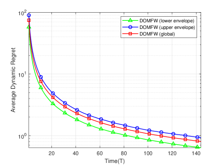
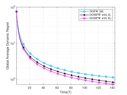
Fig. 1: Three average dynamic regrets under the unit simplex constraint.

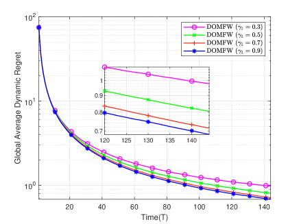
Fig. 2: The comparison results of multiple iterations under the unit simplex constraint.

Fig. 3: The comparison of global average dynamic regret for the unit simplex constraint under different inner number $K_{t}$.

IV-B The Norm Ball Constraint

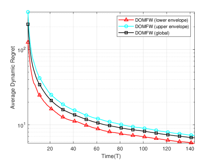
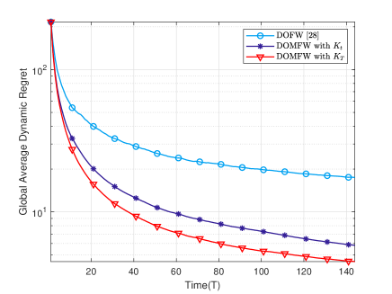
Fig. 4: Three average dynamic regrets of Algorithm 1 under the norm ball constraint.

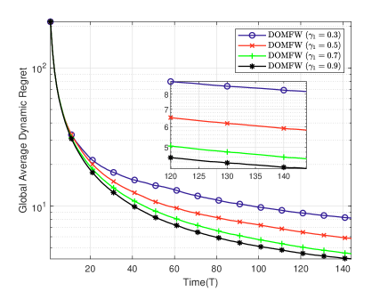
Fig. 5: The comparison results of multiple iterations under the norm ball constraint.

Fig. 6: The comparison of global average dynamic regret for the norm ball constraint under different inner number $K_{t}$.

In this subsection, we study the convergence performance of Algorithm 1 under the norm ball constraint with the dimension $d=16$. Set $\varepsilon_{1}=\varepsilon_{2}=0.3,$ $\gamma_{1}=\gamma_{2}=0.5,\rho=3.5$. Similarly, by observing three regret curves in Fig. 6, we obtain that Algorithm 1 is convergent for this constraint. Next, to verify the effect of the multiple iteration method, we compared DOFW algorithm in [28] and Algorithm 1 under two inner iteration parameters. From Fig. 6, Algorithm DOMFW has better convergence performance than that without multiple iterations [28], which reflects the significant advantages of the multiple iteration method. For two parameter settings $K_{t}$ and $K_{T}$, the performance generated from the latter is better, while the former does not depend on prior knowledge of $T$.

Finally, taking $K_{t}$ as an example, we explore the convergence performance of Algorithm 1 under three different settings of $\gamma_{1}$, i.e., $0.3,0.5,0.7,0.9$ and the settings $\rho=3.5,\varepsilon_{1}=0.3$. Fig. 6 clearly shows that as the order setting of $K_{t}$ over time $t$ increases, the global average dynamic regret of Algorithm 1 is getting better. Similar to Fig. 3, when $\gamma_{1}$ changes from $0.7$ to $0.9$, the improvement of the convergence effect is weak while the increase in the computational cost and communication cost is great. Therefore, as described in the previous section, a proper setting of parameters $\varepsilon_{1}(\text{or}\ \varepsilon_{2})$ and $\gamma_{1}(\text{or}\ \gamma_{2})$ is very important to trade off the relationship between obtaining high-quality decision and saving resources in practical applications.

V Conclusions

For solving the distributed online optimization problem, we have developed the distributed online multiple Frank-Wolfe algorithm over a time-varying multi-agent network. Based on the projection-free operation, the proposed algorithm can significantly save computational cost (at one step), especially for the optimization scenario with a high-dimensional and structural constraint set. Further, we have confirmed that the multiple iteration technique can enhance the dynamic regret bound of the FW algorithm in distributed scenarios. The regret bound $\mathcal{O}(T^{1-\gamma}+H_{T}),0<\gamma<1$ with the linear oracle number $\mathcal{O}(T^{1+\gamma})$ has been established, which is tighter than that without inner iteration loop and does not require a step size dependent on the prior knowledge of $H_{T},T$. In particular, we have confirmed that when the order or estimated order of $H_{T}$ over time $T$ is available, the optimal bound $\mathcal{O}(1+H_{T})$ can be obtained. Moreover, a trade-off between dynamic regret bound, computational cost, and communication cost has been revealed. Finally, we have verified the theoretical results by the simulation of the distributed online ridge regression problems with two constraint sets.

Appendix A Proof of Lemma 1

According to Algorithm 1, by denoting $A_{t}^{K_{t}}$ as the product of ${K_{t}}$ multiplications of $A_{t}$, we get

$${\bm{x}}_{i,t+1}$$

$$=\hat{\bm{x}}_{i,t}^{K_{t}}+\alpha_{t}(\bm{v}_{i,t}^{K_{t}}-\hat{\bm{x}}_{i,t}^{K_{t}})$$

$$=\sum\limits_{j=1}^{n}[A_{t}]_{ij}{\bm{x}}_{j,t}^{K_{t}}+\alpha_{t}\left(\bm{v}_{i,t}^{K_{t}}-\hat{\bm{x}}_{i,t}^{K_{t}}\right)$$

$$=\sum_{j=1}^{n}[A_{t}^{K_{t}}]_{ij}{\bm{x}}_{j,t}+\alpha_{t}\sum\limits_{l=1}^{{K_{t}}-1}\sum\limits_{j=1}^{n}[A_{t}^{{K_{t}}-l}]_{ij}\left(\bm{v}_{j,t}^{l}-\hat{\bm{x}}_{j,t}^{l}\right)$$

$$\quad+\alpha_{t}\left(\bm{v}_{i,t}^{K_{t}}-\hat{\bm{x}}_{i,t}^{K_{t}}\right)$$

$$=\sum_{j=1}^{n}[\Phi^{K}(t,1)]_{ij}{\bm{x}}_{j,1}+\alpha_{t}\left(\bm{v}_{i,t}^{K_{t}}-\hat{\bm{x}}_{i,t}^{K_{t}}\right)$$

$$\quad+\sum_{s=1}^{t}\sum\limits_{l=1}^{{K_{s}}-1}\sum\limits_{j=1}^{n}\alpha_{s}[\Phi^{K}(t,s+1)A_{s}^{{K_{s}}-l}]_{ij}\left(\bm{v}_{j,s}^{l}-\hat{\bm{x}}_{j,s}^{l}\right)$$

$$\quad+\sum_{s=1}^{t-1}\sum_{j=1}^{n}\alpha_{s}[\Phi^{K}(t,s+1)]_{ij}\left(\bm{v}_{j,s}^{K_{s}}-\hat{\bm{x}}_{j,s}^{K_{s}}\right).$$ (42)

According to Algorithm 1, we have that

$$\quad{\bm{x}}_{avg,t}^{K_{t}+1}$$

$$=\frac{1}{n}\sum\limits_{i=1}^{n}\bm{x}_{i,t}^{{K_{t}}+1}$$

$$=\frac{1}{n}\sum\limits_{i=1}^{n}\left[\sum\limits_{j=1}^{n}[A_{t}]_{ij}{\bm{x}}_{j,t}^{K_{t}}+\alpha_{t}\left(\bm{v}_{i,t}^{K_{t}}-\sum\limits_{j=1}^{n}[A_{t}]_{ij}{\bm{x}}_{j,t}^{K_{t}}\right)\right]$$

$$={\bm{x}}_{avg,t}^{K_{t}}+\alpha_{t}({\bm{v}}_{avg,t}^{K_{t}}-{\bm{x}}_{avg,t}^{K_{t}}).$$ (43)

By iteration with respect to $K_{t}$, we further obtain that

$${\bm{x}}_{avg,t}^{K_{t}+1} ={\bm{x}}_{avg,t}+\alpha_{t}\sum\limits_{l=1}^{{K_{t}}}({\bm{v}}_{avg,t}^{l}-{\bm{x}}_{avg,t}^{l}).$$ (44)

Note that ${\bm{x}}_{avg,t+1}={\bm{x}}_{avg,t}^{K_{t}+1}.$ Therefore, we have

$$\quad{\bm{x}}_{avg,t+1}$$

$$={\bm{x}}_{avg,t}+\alpha_{t}\sum\limits_{l=1}^{{K_{t}}}({\bm{v}}_{avg,t}^{l}-{\bm{x}}_{avg,t}^{l})$$

$$={\bm{x}}_{avg,1}+\sum_{s=1}^{t}\sum\limits_{l=1}^{{K_{s}}}\alpha_{s}({\bm{v}}_{avg,s}^{l}-{\bm{x}}_{avg,s}^{l})$$

$$=\frac{1}{n}\sum\limits_{j=1}^{n}{\bm{x}}_{j,1}+\frac{1}{n}\sum_{s=1}^{t}\sum\limits_{l=1}^{{K_{s}}-1}\sum\limits_{j=1}^{n}\alpha_{s}({\bm{v}}_{j,s}^{l}-\hat{\bm{x}}_{j,s}^{l})$$

$$\quad+\frac{1}{n}\sum_{s=1}^{t-1}\sum\limits_{j=1}^{n}\alpha_{s}({\bm{v}}_{j,s}^{K_{s}}-\hat{\bm{x}}_{j,s}^{K_{s}})+\frac{\alpha_{t}}{n}\sum\limits_{j=1}^{n}({\bm{v}}_{j,t}^{K_{t}}-\hat{\bm{x}}_{j,t}^{K_{t}}).$$ (45)

By combining (A) and (A), it follows that

$$\quad\|{\bm{x}}_{i,t+1}-\bm{x}_{avg,t+1}\|$$

$$\leq\sum_{j=1}^{n}\left|[\Phi^{K}(t,1)]_{ij}-\frac{1}{n}\right|\left\|{\bm{x}}_{j,1}\right\|+\alpha_{t}\left\|\bm{v}_{i,t}^{K_{t}}-\hat{\bm{x}}_{i,t}^{K_{t}}\right\|+$$

$$\sum_{s=1}^{t}\sum\limits_{l=1}^{{K_{s}}-1}\sum\limits_{j=1}^{n}\alpha_{s}\left|[\Phi^{K}(t,s+1)A_{s}^{{K_{s}}-l}]_{ij}-\frac{1}{n}\right|\left\|\bm{v}_{j,s}^{l}-\hat{\bm{x}}_{j,s}^{l}\right\|$$

$$\quad+\sum_{s=1}^{t-1}\sum_{j=1}^{n}\alpha_{s}\left|[\Phi^{K}(t,s+1)]_{ij}-\frac{1}{n}\right|\left\|\bm{v}_{j,s}^{K_{s}}-\hat{\bm{x}}_{j,s}^{K_{s}}\right\|$$

$$\quad+\frac{\alpha_{t}}{n}\sum\limits_{j=1}^{n}\left\|{\bm{v}}_{j,t}^{K_{t}}-\hat{\bm{x}}_{j,t}^{K_{t}}\right\|.$$ (46)

Note that, for any appropriate numbers $j,s,l$, the following inequality holds:

$$\left\|{\bm{v}}_{j,s}^{l}-\hat{\bm{x}}_{j,s}^{l}\right\|\leq M.$$ (47)

Then, through recalling (13), (14) and using (47), (A) follows that

$$\quad\|{\bm{x}}_{i,t+1}-\bm{x}_{avg,t+1}\|$$

$$\leq\Gamma_{1}\sigma_{1}^{\sum_{p=1}^{t}K_{p}-1}\sum_{j=1}^{n}\left\|{\bm{x}}_{j,1}\right\|+nM\Gamma_{1}\sum_{s=1}^{t-1}\alpha_{s}\sigma_{1}^{\sum_{p=s+1}^{t}K_{p}-1}$$

$$\quad+nM\Gamma_{1}\sum_{s=1}^{t}\sum\limits_{l=1}^{{K_{s}}-1}\alpha_{s}\sigma_{1}^{\sum_{p=s}^{t}K_{p}-l-1}+2\alpha_{t}M$$

$$\leq\Gamma_{1}\sigma_{1}^{tK_{1}-1}\sum_{j=1}^{n}\left\|{\bm{x}}_{j,1}\right\|+nM\Gamma_{1}\sum_{s=1}^{t}\alpha_{s}\sigma_{1}^{(t-s)K_{1}-1}$$

$$\quad+nM\Gamma_{1}\sum_{s=1}^{t}\sum\limits_{l=1}^{{K_{s}}-1}\alpha_{s}\sigma_{1}^{(t-s)K_{1}+K_{t}-l-1}+2\alpha_{t}M$$ (48)

where in the last inequality we use the non-decreasing property of the sequence $\{K_{t}\}$. Based on (A), we can further obtain that

$$\quad\sum\limits_{t=1}^{T}\sum\limits_{i=1}^{n}\|{\bm{x}}_{i,t}-\bm{x}_{avg,t}\|$$

$$=\sum_{t=1}^{T-1}\sum\limits_{i=1}^{n}\|{\bm{x}}_{i,t+1}-\bm{x}_{avg,t+1}\|+\sum\limits_{i=1}^{n}\|{\bm{x}}_{i,1}-\bm{x}_{avg,1}\|$$

$$\leq n\Gamma_{1}\sum_{t=1}^{T-1}\sigma_{1}^{tK_{1}-1}\sum_{j=1}^{n}\left\|{\bm{x}}_{j,1}\right\|+\sum\limits_{i=1}^{n}\|{\bm{x}}_{i,1}-\bm{x}_{avg,1}\|$$

$$\quad+n^{2}M\Gamma_{1}\sum_{t=1}^{T-1}\sum_{s=1}^{t}\sum\limits_{l=1}^{{K_{s}}-1}\alpha_{s}\sigma_{1}^{(t-s)K_{1}+K_{t}-l-1}$$

$$\quad+n^{2}M\Gamma_{1}\sum_{t=1}^{T-1}\sum_{s=1}^{t}\alpha_{s}\sigma_{1}^{(t-s)K_{1}-1}+2nM\sum_{t=1}^{T-1}\alpha_{t}.$$ (49)

Now, we are going to handle the summations involved in (A). Recalling that $0<\sigma_{1}<1$ and $K_{1}\geq 2$, we have

$$\sum_{t=1}^{T-1}\sigma_{1}^{tK_{1}-1}=\frac{1}{\sigma_{1}}\sum_{t=1}^{T-1}\left(\sigma_{1}^{K_{1}}\right)^{t}\leq\frac{\sigma_{1}^{K_{1}}}{\sigma_{1}\left(1-\sigma_{1}^{K_{1}}\right)}\leq\frac{1}{1-\sigma_{1}^{K_{1}}}.$$ (50)

Note that the sequence $\{K_{t}\}$ is non-decreasing. Then, it is not difficult to obtain that

$$\quad\sum_{t=1}^{T-1}\sum_{s=1}^{t}\sum\limits_{l=1}^{{K_{s}}-1}\alpha_{s}\sigma_{1}^{(t-s)K_{1}+K_{t}-l-1}$$

$$\leq\sum_{t=1}^{T-1}\sum_{s=1}^{t}\alpha_{s}\sigma_{1}^{(t-s)K_{1}}\sum\limits_{l=1}^{{K_{t}}-1}\sigma_{1}^{K_{t}-l-1}$$

$$\leq\frac{1}{1-{\sigma_{1}}}\sum_{t=1}^{T-1}\sum_{s=1}^{t}\alpha_{s}{\sigma_{1}}^{(t-s){K_{1}}}$$

$$\leq\frac{1}{1-{\sigma_{1}}}\left(\sum_{t=1}^{T}\alpha_{t}\right)\left(\sum_{s=1}^{T}{\sigma_{1}}^{(s-1){K_{1}}}\right)$$

$$\leq\frac{1}{\left(1-{\sigma_{1}}\right)\left(1-{\sigma_{1}}^{K_{1}}\right)}\sum\limits_{t=1}^{T}\alpha_{t}.$$ (51)

Similarly, it can be verified that

$$\sum_{t=1}^{T-1}\sum_{s=1}^{t}\alpha_{s}\sigma_{1}^{(t-s)K_{1}-1} \leq\frac{1}{{\sigma_{1}}\left(1-{\sigma_{1}}^{K_{1}}\right)}\sum\limits_{t=1}^{T}\alpha_{t}.$$ (52)

Combining (A)-(52) yields the condition in (1). The proof is complete. $\square$

Appendix B Proof of Lemma 2

Under Assumption 4, we have

$$\quad\left\|\widehat{\nabla}f_{i,t}^{k}-\frac{1}{n}\nabla F_{t}({\bm{x}}_{avg,t}^{k})\right\|$$

$$\leq\left\|\widehat{\nabla}f_{i,t}^{k}-\frac{1}{n}\sum\limits_{i=1}^{n}\nabla f_{i,t}(\hat{\bm{x}}_{i,t}^{k})\right\|$$

$$\quad+\left\|\frac{1}{n}\sum\limits_{i=1}^{n}\nabla f_{i,t}(\hat{\bm{x}}_{i,t}^{k})-\frac{1}{n}\nabla F_{t}({\bm{x}}_{avg,t}^{k})\right\|$$

$$\leq\left\|\widehat{\nabla}f_{i,t}^{k}-\frac{1}{n}\sum\limits_{i=1}^{n}\nabla f_{i,t}(\hat{\bm{x}}_{i,t}^{k})\right\|+\frac{G_{X}}{n}\sum\limits_{i=1}^{n}\left\|\hat{\bm{x}}_{i,t}^{k}-{\bm{x}}_{avg,t}^{k}\right\|$$

$$\leq\left\|\widehat{\nabla}f_{i,t}^{k}-\frac{1}{n}\sum\limits_{i=1}^{n}\nabla f_{i,t}(\hat{\bm{x}}_{i,t}^{k})\right\|+\frac{G_{X}}{n}\sum\limits_{i=1}^{n}\left\|{\bm{x}}_{i,t}^{k}-{\bm{x}}_{avg,t}^{k}\right\|$$ (53)

where the last inequality is obtained by using the double stochasticity of $A_{t}$. Then, after summing (B) with respect to $i,k$ and $t$, we have

$$\quad\sum\limits_{t=1}^{T}\sum_{k=1}^{K_{t}}\sum\limits_{i=1}^{n}\alpha_{t}\left\|\widehat{\nabla}f_{i,t}^{k}-\frac{1}{n}\nabla F_{t}({\bm{x}}_{avg,t}^{k})\right\|$$

$$\leq\sum\limits_{t=1}^{T}\sum_{k=1}^{K_{t}}\sum\limits_{i=1}^{n}\alpha_{t}\left\|\widehat{\nabla}f_{i,t}^{k}-\frac{1}{n}\sum\limits_{i=1}^{n}\nabla f_{i,t}(\hat{\bm{x}}_{i,t}^{k})\right\|$$

$$\quad+G_{X}\sum\limits_{t=1}^{T}\sum_{k=1}^{K_{t}}\sum\limits_{i=1}^{n}\alpha_{t}\left\|{\bm{x}}_{i,t}^{k}-{\bm{x}}_{avg,t}^{k}\right\|.$$ (54)

The first term on the right hand side is first analysed.

$$\quad\widehat{\nabla}f_{i,t}^{k}$$

$$=\sum\limits_{j=1}^{n}[A_{t}]_{ij}\overline{\nabla}f_{j,t}^{k}$$

$$=\sum\limits_{j=1}^{n}[A_{t}]_{ij}\widehat{\nabla}f_{j,t}^{k-1}+\sum\limits_{j=1}^{n}[A_{t}]_{ij}\delta_{j,t}^{k-1}$$

$$=\sum\limits_{j=1}^{n}[A_{t}^{k}]_{ij}{\nabla}f_{j,t}(\hat{\bm{x}}_{j,t}^{1})+\sum\limits_{l=2}^{k}\sum\limits_{j=1}^{n}[A_{t}^{k-l+1}]_{ij}\delta_{j,t}^{l-1}.$$ (55)

Based on Algorithm 1, it is easily obtained that $\sum_{i=1}^{n}\overline{\nabla}f_{i,1}^{1}=\sum_{i=1}^{n}\nabla f_{i,1}(\hat{\bm{x}}_{i,1}^{1})$. Now we assume that $\sum_{i=1}^{n}\overline{\nabla}f_{i,t}^{k-1}=\sum_{i=1}^{n}\nabla f_{i,t}(\hat{\bm{x}}_{i,t}^{k-1})$ holds. Then, we intend to prove the equality also hold at time $t+1$. Actually,

$$\quad\sum\limits_{i=1}^{n}\overline{\nabla}f_{i,t}^{k}$$

$$=\sum\limits_{i=1}^{n}\widehat{\nabla}f_{i,t}^{k-1}+\sum\limits_{i=1}^{n}\nabla f_{i,t}(\hat{\bm{x}}_{i,t}^{k})-\sum\limits_{i=1}^{n}\nabla f_{i,t}(\hat{\bm{x}}_{i,t}^{k-1})$$

$$=\sum\limits_{i=1}^{n}\sum_{j=1}^{n}[A_{t}]_{ij}\overline{\nabla}f_{j,t}^{k-1}+\sum\limits_{i=1}^{n}\nabla f_{i,t}(\hat{\bm{x}}_{i,t}^{k})-\sum_{i=1}^{n}\overline{\nabla}f_{i,t}^{k-1}$$

$$=\sum\limits_{i=1}^{n}\nabla f_{i,t}(\hat{\bm{x}}_{i,t}^{k})$$ (56)

where the third equality combines the double stochasticity of $A_{t}$.

This further gives that

$$\quad\frac{1}{n}\sum\limits_{i=1}^{n}{\nabla}f_{i,t}(\hat{\bm{x}}_{i,t}^{k})$$

$$=\frac{1}{n}\sum\limits_{i=1}^{n}\sum\limits_{j=1}^{n}[A_{t}]_{ij}\overline{\nabla}f_{j,t}^{k-1}+\frac{1}{n}\sum\limits_{i=1}^{n}\delta_{i,t}^{k-1}$$

$$=\frac{1}{n}\sum\limits_{i=1}^{n}\nabla f_{i,t}(\hat{\bm{x}}_{i,t}^{k-1})+\frac{1}{n}\sum\limits_{i=1}^{n}\delta_{i,t}^{k-1}$$

$$=\frac{1}{n}\sum\limits_{i=1}^{n}{\nabla}f_{i,t}(\hat{\bm{x}}_{i,t}^{1})+\frac{1}{n}\sum\limits_{l=2}^{k}\sum\limits_{i=1}^{n}\delta_{i,t}^{l-1}.$$ (57)

Based on the above analysis, we obtain that, for any $k\geq 2$,

$$\quad\left\|\widehat{\nabla}f_{i,t}^{k}-\frac{1}{n}\sum\limits_{i=1}^{n}{\nabla}f_{i,t}(\hat{\bm{x}}_{i,t}^{k})\right\|$$

$$\leq\sum\limits_{j=1}^{n}\left|[A_{t}^{k}]_{ij}-\frac{1}{n}\right|\left\|{\nabla}f_{j,t}(\hat{\bm{x}}_{j,t}^{1})\right\|$$

$$\quad+\sum\limits_{l=2}^{k}\sum\limits_{j=1}^{n}\left|[A_{t}^{k-l+1}]_{ij}-\frac{1}{n}\right|\left\|\delta_{j,t}^{l-1}\right\|$$

$$\leq\Gamma_{1}{\sigma_{1}}^{k-1}\sum\limits_{j=1}^{n}\left\|{\nabla}f_{j,t}(\hat{\bm{x}}_{j,t}^{1})\right\|+\Gamma_{1}\sum\limits_{l=2}^{k}\sum\limits_{j=1}^{n}{\sigma_{1}}^{k-l}\left\|\delta_{j,t}^{l-1}\right\|.$$ (58)

This implies that

$$\quad\sum_{k=1}^{K_{t}}\sum\limits_{i=1}^{n}\left\|\widehat{\nabla}f_{i,t}^{k}-\frac{1}{n}\sum\limits_{i=1}^{n}{\nabla}f_{i,t}(\hat{\bm{x}}_{i,t}^{k})\right\|$$

$$=\sum\limits_{i=1}^{n}\left\|\widehat{\nabla}f_{i,t}^{1}-\frac{1}{n}\sum\limits_{i=1}^{n}{\nabla}f_{i,t}(\hat{\bm{x}}_{i,t}^{1})\right\|$$

$$\quad+\sum_{k=2}^{K_{t}}\sum\limits_{i=1}^{n}\left\|\widehat{\nabla}f_{i,t}^{k}-\frac{1}{n}\sum\limits_{i=1}^{n}{\nabla}f_{i,t}(\hat{\bm{x}}_{i,t}^{k})\right\|$$

$$\leq\sum\limits_{i=1}^{n}\left\|\widehat{\nabla}f_{i,t}^{1}-\frac{1}{n}\sum\limits_{i=1}^{n}{\nabla}f_{i,t}(\hat{\bm{x}}_{i,t}^{1})\right\|+n\Gamma_{1}\sum\limits_{k=2}^{K_{t}}\sum\limits_{j=1}^{n}{\sigma_{1}}^{k-1}\cdot$$

$$\quad\left\|{\nabla}f_{j,t}(\hat{\bm{x}}_{j,t}^{1})\right\|+n\Gamma_{1}\sum\limits_{k=2}^{K_{t}}\sum\limits_{l=2}^{k}\sum\limits_{j=1}^{n}{\sigma_{1}}^{k-l}\left\|\delta_{j,t}^{l-1}\right\|.$$ (59)

Now we are going to estimate the bounds of the terms in (B). Firstly, we have

$$\quad\sum\limits_{i=1}^{n}\left\|\widehat{\nabla}f_{i,t}^{1}-\frac{1}{n}\sum\limits_{i=1}^{n}{\nabla}f_{i,t}(\hat{\bm{x}}_{i,t}^{1})\right\|$$

$$=\sum\limits_{i=1}^{n}\left\|\sum\limits_{j=1}^{n}[A_{t}]_{ij}{\nabla}f_{j,t}(\hat{\bm{x}}_{j,t}^{1})-\frac{1}{n}\sum\limits_{j=1}^{n}\nabla f_{j,t}(\hat{\bm{x}}_{j,t}^{1})\right\|$$

$$\leq\sum\limits_{i=1}^{n}\sum\limits_{j=1}^{n}\left|[A_{t}]_{ij}-\frac{1}{n}\right|\left\|{\nabla}f_{j,t}(\hat{\bm{x}}_{j,t}^{1})\right\|$$

$$\leq n^{2}\Gamma_{1}L_{X}.$$ (60)

Next, it is easily obtained that

$$n\Gamma_{1}\sum\limits_{k=2}^{K_{t}}\sum\limits_{j=1}^{n}{\sigma_{1}}^{k-1}\left\|{\nabla}f_{j,t}(\hat{\bm{x}}_{j,t}^{1})\right\| \leq\frac{{\sigma_{1}}n^{2}\Gamma_{1}L_{X}}{1-{\sigma_{1}}}.$$ (61)

Moreover, it can be verified that

$$\quad n\Gamma_{1}\sum\limits_{k=2}^{K_{t}}\sum\limits_{l=2}^{k}\sum\limits_{j=1}^{n}{\sigma_{1}}^{k-l}\left\|\delta_{j,t}^{l-1}\right\|$$

$$\leq n\Gamma_{1}\left(\sum\limits_{k=2}^{{K_{t}}}{\sigma_{1}}^{k-2}\right)\left(\sum\limits_{k=2}^{{K_{t}}}\sum\limits_{i=1}^{n}\left\|\delta_{i,t}^{k-1}\right\|\right)$$

$$\leq\frac{n\Gamma_{1}}{1-{\sigma_{1}}}\sum\limits_{k=1}^{{K_{t}}-1}\sum\limits_{i=1}^{n}\left\|\nabla f_{i,t}(\hat{\bm{x}}_{i,t}^{k+1})-\nabla f_{i,t}(\hat{\bm{x}}_{i,t}^{k})\right\|$$

$$\leq\frac{n\Gamma_{1}G_{X}}{1-{\sigma_{1}}}\sum\limits_{k=1}^{{K_{t}}-1}\sum\limits_{i=1}^{n}\left\|\hat{\bm{x}}_{i,t}^{k+1}-\hat{\bm{x}}_{i,t}^{k}\right\|.$$ (62)

Note that

$$\quad\sum\limits_{i=1}^{n}\left\|\hat{\bm{x}}_{i,t}^{k+1}-\hat{\bm{x}}_{i,t}^{k}\right\|$$

$$\leq\sum\limits_{i=1}^{n}\left\|\hat{\bm{x}}_{i,t}^{k+1}-{\bm{x}}_{avg,t}^{k}\right\|+\sum\limits_{i=1}^{n}\left\|{\bm{x}}_{avg,t}^{k}-\hat{\bm{x}}_{i,t}^{k}\right\|$$

$$\leq\sum\limits_{i=1}^{n}\left\|{\bm{x}}_{i,t}^{k+1}-{\bm{x}}_{avg,t}^{k}\right\|+\sum\limits_{i=1}^{n}\left\|{\bm{x}}_{avg,t}^{k}-{\bm{x}}_{i,t}^{k}\right\|$$

$$\leq\sum\limits_{i=1}^{n}\left\|\hat{\bm{x}}_{i,t}^{k}+\alpha_{t}(\bm{v}_{i,t}^{k}-\hat{\bm{x}}_{i,t}^{k})-{\bm{x}}_{avg,t}^{k}\right\|+\sum\limits_{i=1}^{n}\left\|{\bm{x}}_{avg,t}^{k}-{\bm{x}}_{i,t}^{k}\right\|$$

$$\leq 2\sum\limits_{i=1}^{n}\left\|{\bm{x}}_{i,t}^{k}-{\bm{x}}_{avg,t}^{k}\right\|+\alpha_{t}nM.$$ (63)

This, together with (62), implies that

$$\quad n\Gamma_{1}\sum\limits_{k=2}^{K_{t}}\sum\limits_{l=2}^{k}\sum\limits_{j=1}^{n}{\sigma_{1}}^{k-l}\left\|\delta_{j,t}^{l-1}\right\|$$

$$\leq\frac{2n\Gamma_{1}G_{X}}{1-{\sigma_{1}}}\sum\limits_{k=1}^{{K_{t}}-1}\sum\limits_{i=1}^{n}\left\|{\bm{x}}_{i,t}^{k}-{\bm{x}}_{avg,t}^{k}\right\|+\frac{n^{2}\Gamma_{1}G_{X}M}{1-{\sigma_{1}}}\alpha_{t}{K_{t}}.$$ (64)

Then, substituting (60), (61) and (64) into (B), we have

$$\quad\sum\limits_{t=1}^{T}\alpha_{t}\sum_{k=1}^{K_{t}}\sum\limits_{i=1}^{n}\left\|\widehat{\nabla}f_{i,t}^{k}-\frac{1}{n}\sum\limits_{i=1}^{n}\nabla f_{i,t}(\hat{\bm{x}}_{i,t}^{k})\right\|$$

$$\leq\frac{n^{2}\Gamma_{1}L_{X}}{1-{\sigma_{1}}}\sum\limits_{t=1}^{T}\alpha_{t}+\frac{n^{2}\Gamma_{1}G_{X}M}{1-{\sigma_{1}}}\sum\limits_{t=1}^{T}\alpha_{t}^{2}{K_{t}}$$

$$\quad+\frac{2n\Gamma_{1}G_{X}}{1-{\sigma_{1}}}\sum\limits_{t=1}^{T}\sum\limits_{k=1}^{{K_{t}}-1}\sum\limits_{i=1}^{n}\alpha_{t}\left\|{\bm{x}}_{i,t}^{k}-{\bm{x}}_{avg,t}^{k}\right\|.$$ (65)

On the other hand, similar to Lemma 1, we easily obtain the following results:

$${\bm{x}}_{i,t}^{k+1} =\sum_{j=1}^{n}[A_{t}^{k}]_{ij}{\bm{x}}_{j,t}^{1}+\alpha_{t}\sum\limits_{l=1}^{k-1}\sum\limits_{j=1}^{n}[A_{t}^{k-l}]_{ij}\left(\bm{v}_{j,t}^{l}-\hat{\bm{x}}_{j,t}^{l}\right)$$

$$\quad+\alpha_{t}\left(\bm{v}_{i,t}^{k}-\hat{\bm{x}}_{i,t}^{k}\right),$$ (66)

$$\bm{x}_{avg,t}^{k+1} =\frac{1}{n}\sum\limits_{i=1}^{n}{\bm{x}}_{i,t}^{1}+\frac{\alpha_{t}}{n}\sum\limits_{l=1}^{k-1}\sum\limits_{i=1}^{n}({\bm{v}}_{i,t}^{l}-\hat{\bm{x}}_{i,t}^{l})$$

$$\quad+\alpha_{t}({\bm{v}}_{avg,t}^{k}-{\bm{x}}_{avg,t}^{k}).$$ (67)

Based on these two conditions, we further obtain that

$$\quad\left\|{\bm{x}}_{i,t}^{k+1}-\bm{x}_{avg,t}^{k+1}\right\|$$

$$\leq\sum_{j=1}^{n}\left|[A_{t}^{k}]_{ij}-\frac{1}{n}\right|\left\|{\bm{x}}_{j,t}^{1}\right\|$$

$$\quad+\alpha_{t}\sum\limits_{l=1}^{k-1}\sum\limits_{j=1}^{n}\left|[A_{t}^{k-l}]_{ij}-\frac{1}{n}\right\|\left\|{\bm{v}}_{i,t}^{l}-\hat{\bm{x}}_{i,t}^{l}\right\|+2\alpha_{t}M$$

$$\leq\Gamma_{1}{\sigma_{1}}^{k-1}\sum_{j=1}^{n}\left\|{\bm{x}}_{j,t}^{1}\right\|+\alpha_{t}nM\Gamma_{1}\sum\limits_{l=1}^{k-1}{\sigma_{1}}^{k-l-1}+2\alpha_{t}M$$

$$=\Gamma_{1}{\sigma_{1}}^{k-1}\sum_{j=1}^{n}\left\|{\bm{x}}_{j,t}^{1}-{\bm{x}}_{j,1}+{\bm{x}}_{j,1}\right\|+\alpha_{t}n\Gamma_{1}M\sum\limits_{s=1}^{k-1}{\sigma_{1}}^{s-1}$$

$$\quad+2\alpha_{t}M$$

$$\leq nM\Gamma_{1}{\sigma_{1}}^{k-1}+\Gamma_{1}{\sigma_{1}}^{k-1}\sum_{j=1}^{n}\left\|{\bm{x}}_{j,1}\right\|+\alpha_{t}n\Gamma_{1}M\sum\limits_{s=1}^{k-1}{\sigma_{1}}^{s-1}$$

$$\quad+2\alpha_{t}M.$$ (68)

Summing (68) with respect to $i,k$ and $t$, we have

$$\quad\sum_{t=1}^{T}\sum_{k=1}^{K_{t}}\sum_{i=1}^{n}\alpha_{t}\|{\bm{x}}_{i,t}^{k}-{\bm{x}}_{avg,t}^{k}\|$$

$$\leq\sum_{t=1}^{T}\sum_{i=1}^{n}\alpha_{t}\|{\bm{x}}_{i,t}^{1}-{\bm{x}}_{avg,t}^{1}\|+\sum_{t=1}^{T}\sum_{k=2}^{K_{t}}\sum_{i=1}^{n}\alpha_{t}\|{\bm{x}}_{i,t}^{k}-{\bm{x}}_{avg,t}^{k}\|$$

$$\leq nM\sum_{t=1}^{T}\alpha_{t}+n^{2}M\Gamma_{1}\sum_{t=1}^{T}\sum_{k=2}^{K_{t}}{\sigma_{1}}^{k-2}\alpha_{t}$$

$$\quad+n\Gamma_{1}\sum_{t=1}^{T}\sum_{k=2}^{K_{t}}\sum_{j=1}^{n}{\sigma_{1}}^{k-2}\alpha_{t}\|\bm{x}_{j,1}\|$$

$$\quad+n^{2}\Gamma_{1}M\sum_{t=1}^{T}\sum_{k=2}^{K_{t}}\sum\limits_{s=1}^{k-1}{\sigma_{1}}^{s-1}\alpha_{t}^{2}+2nM\sum_{t=1}^{T}\alpha_{t}^{2}{K_{t}}$$

$$\leq\left[nM+\frac{n\Gamma_{1}}{1-{\sigma_{1}}}\sum_{j=1}^{n}(\|\bm{x}_{j,1}\|+M)\right]\sum_{t=1}^{T}\alpha_{t}$$

$$\quad+\left(\frac{n^{2}\Gamma_{1}M}{1-{\sigma_{1}}}+2nM\right)\sum\limits_{t=1}^{T}\alpha_{t}^{2}{K_{t}}.$$ (69)

Combining (B), (B) and (B) yields (2). The proof is complete. $\square$

Appendix C Proof of Lemma 3

Based on Algorithm 1 and the smooth property in Assumption 4, we have

$$\quad F_{t}\left(\bm{x}_{avg,t}^{k+1}\right)-F_{t}\left(\bm{x}_{avg,t}^{k}\right)$$

$$\leq\left<\nabla F_{t}\left(\bm{x}_{avg,t}^{k}\right),\bm{x}_{avg,t}^{k+1}-\bm{x}_{avg,t}^{k}\right>+\frac{nG_{X}}{2}\left\|\bm{x}_{avg,t}^{k+1}-\bm{x}_{avg,t}^{k}\right\|^{2}$$

$$=\alpha_{t}\left<\nabla F_{t}\left(\bm{x}_{avg,t}^{k}\right),\bm{v}_{avg,t}^{k}-\bm{x}_{avg,t}^{k}\right>$$

$$\quad+\frac{n\alpha_{t}^{2}G_{X}}{2}\left\|\bm{v}_{avg,t}^{k}-\bm{x}_{avg,t}^{k}\right\|^{2}$$

$$\leq\alpha_{t}\sum\limits_{i=1}^{n}\left<\frac{1}{n}\nabla F_{t}\left(\bm{x}_{avg,t}^{k}\right),\bm{v}_{i,t}^{k}-\bm{x}_{avg,t}^{k}\right>+\frac{n\alpha_{t}^{2}G_{X}M^{2}}{2}$$ (70)

where we used the fact $\bm{x}_{avg,t}^{k+1}=\bm{x}_{avg,t}^{k}+\alpha_{t}(\bm{v}_{avg,t}^{k}-\bm{x}_{avg,t}^{k})$. Furthermore, it is noted that

$$\quad\left<\frac{1}{n}\nabla F_{t}\left(\bm{x}_{avg,t}^{k}\right),\bm{v}_{i,t}^{k}-\bm{x}_{avg,t}^{k}\right>$$

$$\leq\left<\frac{1}{n}\nabla F_{t}\left(\bm{x}_{avg,t}^{k}\right)-\widehat{\nabla}f_{i,t}^{k},\bm{v}_{i,t}^{k}-\bm{x}_{avg,t}^{k}\right>$$

$$\quad+\left<\widehat{\nabla}f_{i,t}^{k},\bm{x}_{t}^{*}-\bm{x}_{avg,t}^{k}\right>$$

$$\leq 2M\left\|\frac{1}{n}\nabla F_{t}\left(\bm{x}_{avg,t}^{k}\right)-\widehat{\nabla}f_{i,t}^{k}\right\|$$

$$\quad+\left<\frac{1}{n}\nabla F_{t}\left(\bm{x}_{avg,t}^{k}\right),\bm{x}_{t}^{*}-\bm{x}_{avg,t}^{k}\right>$$

$$\leq 2M\left\|\frac{1}{n}\nabla F_{t}\left(\bm{x}_{avg,t}^{k}\right)-\widehat{\nabla}f_{i,t}^{k}\right\|+\frac{1}{n}\left[F_{t}\left(\bm{x}_{t}^{*}\right)-F_{t}\left(\bm{x}_{avg,t}^{k}\right)\right]$$ (71)

where the first inequality and the last inequality utilize the optimality condition of the variable $\bm{v}_{i,t}^{k}$ and the convexity condition of $F_{t}(\bm{x})$, respectively. Subtracting the term $F_{t}(x_{t}^{*})$ from both sides of (C) and substituting (C) into (C), the following inequality is obtained:

$$\quad F_{t}\left(\bm{x}_{avg,t}^{k+1}\right)-F_{t}(x_{t}^{*})$$

$$=F_{t}\left(\bm{x}_{avg,t}^{k+1}\right)-F_{t}\left(\bm{x}_{avg,t}^{k}\right)+F_{t}\left(\bm{x}_{avg,t}^{k}\right)-F_{t}(x_{t}^{*})$$

$$\leq(1-\alpha_{t})\left[F_{t}\left(\bm{x}_{avg,t}^{k}\right)-F_{t}(x_{t}^{*})\right]$$

$$\quad+2\alpha_{t}M\sum\limits_{i=1}^{n}\left\|\frac{1}{n}\nabla F_{t}\left(\bm{x}_{avg,t}^{k}\right)-\widehat{\nabla}f_{i,t}^{k}\right\|+\frac{n\alpha_{t}^{2}G_{X}M^{2}}{2}$$

$$=(1-\alpha_{t})^{k}\left[F_{t}\left(\bm{x}_{avg,t}^{1}\right)-F_{t}(x_{t}^{*})\right]$$

$$\quad+2\alpha_{t}M\sum_{l=0}^{k-1}(1-\alpha_{t})^{l}\sum\limits_{i=1}^{n}\left\|\frac{1}{n}\nabla F_{t}\left(\bm{x}_{avg,t}^{k-l}\right)-\widehat{\nabla}f_{i,t}^{k-l}\right\|$$

$$\quad+\frac{n\alpha_{t}^{2}G_{X}M^{2}}{2}\sum_{l=0}^{k-1}(1-\alpha_{t})^{l}$$

$$\leq(1-\alpha_{t})^{k}\left[F_{t}\left(\bm{x}_{avg,t}^{1}\right)-F_{t}(x_{t}^{*})\right]$$

$$\quad+2\alpha_{t}M\sum_{l=1}^{k}\sum\limits_{i=1}^{n}\left\|\frac{1}{n}\nabla F_{t}\left(\bm{x}_{avg,t}^{l}\right)-\widehat{\nabla}f_{i,t}^{l}\right\|+\frac{n\alpha_{t}G_{X}M^{2}}{2}$$ (72)

where in the last inequality we utilize the two facts $(1-\alpha_{t})^{l}\leq 1$ and $\sum_{l=0}^{k-1}(1-\alpha_{t})^{l}\leq\frac{1}{\alpha_{t}}$. The proof is complete. $\square$

References

- [1] S. Shalev-Shwartz, “Online learning and online convex optimization,” Foundations and Trends in Machine Learning, vol. 4, no. 2, pp. 107–194, 2011.
- [2] E. Hazan, “Introduction to online convex optimization,” Foundations and Trends® in Optimization, vol. 2, no. 3-4, pp. 157–325, 2016.
- [3] A. Nedić, A. Olshevsky, A. Ozdaglar, and J. N. Tsitsiklis, “Distributed subgradient methods and quantization effects,” in 2008 47th IEEE Conference on Decision and Control, 2008, pp. 4177–4184.
- [4] A. Nedić and J. Liu, “Distributed optimization for control,” Annual Review of Control, Robotics, and Autonomous Systems, vol. 1, pp. 77–103, 2018.
- [5] T. Yang, X. Yi, J. Wu, Y. Yuan, D. Wu, Z. Meng, Y. Hong, H. Wang, Z. Lin, and K. H. Johansson, “A survey of distributed optimization,” Annual Reviews in Control, vol. 47, pp. 278–305, 2019.
- [6] X. Li, L. Xie, and N. Li, “A survey of decentralized online learning,” arXiv preprint arXiv:2205.00473, 2022.
- [7] J. Zhang, K. You, and L. Xie, “Innovation compression for communication-efficient distributed optimization with linear convergence,” IEEE Transactions on Automatic Control, 2023, doi:10.1109/TAC.2023.3241771.
- [8] C. Liu, H. Li, and Y. Shi, “A unitary distributed subgradient method for multi-agent optimization with different coupling sources,” Automatica, vol. 114, p. 108834, 2020.
- [9] W. Li, X. Zeng, Y. Hong, and H. Ji, “Distributed consensus-based solver for semi-definite programming: An optimization viewpoint,” Automatica, vol. 131, p. 109737, 2021.
- [10] J.-M. Xu and Y. C. Soh, “A distributed simultaneous perturbation approach for large-scale dynamic optimization problems,” Automatica, vol. 72, pp. 194–204, 2016.
- [11] F. Yan, S. Sundaram, S. Vishwanathan, and Y. Qi, “Distributed autonomous online learning: Regrets and intrinsic privacy-preserving properties,” IEEE Transactions on Knowledge and Data Engineering, vol. 25, no. 11, pp. 2483–2493, 2013.
- [12] S. Hosseini, A. Chapman, and M. Mesbahi, “Online distributed optimization via dual averaging,” in 52nd IEEE Conference on Decision and Control. IEEE, 2013, pp. 1484–1489.
- [13] D. Yuan, B. Zhang, D. W. Ho, W. X. Zheng, and S. Xu, “Distributed online bandit optimization under random quantization,” Automatica, vol. 146, p. 110590, 2022.
- [14] X. Yi, X. Li, L. Xie, and K. H. Johansson, “Distributed online convex optimization with time-varying coupled inequality constraints,” IEEE Transactions on Signal Processing, vol. 68, pp. 731–746, 2020.
- [15] X. Cao and T. Başar, “Distributed constrained online convex optimization over multiple access fading channels,” IEEE Transactions on Signal Processing, vol. 70, pp. 3468–3483, 2022.
- [16] S. Shahrampour and A. Jadbabaie, “Distributed online optimization in dynamic environments using mirror descent,” IEEE Transactions on Automatic Control, vol. 63, no. 3, pp. 714–725, 2017.
- [17] D. Yuan, Y. Hong, D. W. Ho, and S. Xu, “Distributed mirror descent for online composite optimization,” IEEE Transactions on Automatic Control, vol. 66, no. 2, pp. 714–729, 2020.
- [18] C. Wang, S. Xu, D. Yuan, B. Zhang, and Z. Zhang, “Push-sum distributed online optimization with bandit feedback,” IEEE Transactions on Cybernetics, vol. 52, no. 4, pp. 2263–2273, 2020.
- [19] M. Zinkevich, “Online convex programming and generalized infinitesimal gradient ascent,” in Proceedings of the 20th international conference on machine learning (icml-03), 2003, pp. 928–936.
- [20] O. Besbes, Y. Gur, and A. Zeevi, “Non-stationary stochastic optimization,” Operations Research, vol. 63, no. 5, pp. 1227–1244, 2015.
- [21] Z. Xu, H. Zhou, and V. Tzoumas, “Online submodular coordination with bounded tracking regret: Theory, algorithm, and applications to multi-robot coordination,” IEEE Robotics and Automation Letters, vol. 8, no. 4, pp. 2261–2268, 2023.
- [22] W. Zhang, P. Zhao, W. Zhu, S. C. H. Hoi, and T. Zhang, “Projection-free distributed online learning in networks,” in Proceedings of the 34th International Conference on Machine Learning, 2017, pp. 4054–4062.
- [23] Y. Wan, W.-W. Tu, and L. Zhang, “Projection-free distributed online convex optimization with communication complexity,” in Proceedings of the 37th International Conference on Machine Learning, 2020, pp. 9818–9828.
- [24] Y. Wan, G. Wang, and L. Zhang, “Projection-free distributed online learning with strongly convex losses,” arXiv preprint arXiv:2103.11102, 2021.
- [25] N. K. Thang, A. Srivastav, D. Trystram, and P. Youssef, “A stochastic conditional gradient algorithm for decentralized online convex optimization,” Journal of Parallel and Distributed Computing, vol. 169, pp. 334–351, 2022.
- [26] D. S. Kalhan, A. S. Bedi, A. Koppel, K. Rajawat, H. Hassani, A. K. Gupta, and A. Banerjee, “Dynamic online learning via Frank-Wolfe algorithm,” IEEE Transactions on Signal Processing, vol. 69, pp. 932–947, 2021.
- [27] Y. Wan, B. Xue, and L. Zhang, “Projection-free online learning in dynamic environments,” in Proceedings of the AAAI Conference on Artificial Intelligence, 2021, pp. 10 067–10 075.
- [28] W. Zhang, Y. Shi, B. Zhang, and D. Yuan, “Dynamic regret of distributed online Frank-Wolfe convex optimization,” arXiv preprint arXiv:2302.00663, 2023.
- [29] E. Hazan and S. Kale, “Projection-free online learning,” in Proceedings of the 29th International Coference on International Conference on Machine Learning, 2012, pp. 1843–1850.
- [30] E. Hazan, “Sparse approximate solutions to semidefinite programs,” in Latin American Symposium on Theoretical Informatics, 2008, pp. 306–316.
- [31] Z. Harchaoui, A. Juditsky, and A. Nemirovski, “Conditional gradient algorithms for norm-regularized smooth convex optimization,” Mathematical Programming, vol. 152, no. 1-2, pp. 75–112, 2015.
- [32] H.-T. Wai, J. Lafond, A. Scaglione, and E. Moulines, “Decentralized Frank-Wolfe algorithm for convex and nonconvex problems,” IEEE Transactions on Automatic Control, vol. 62, no. 11, pp. 5522–5537, 2017.
- [33] F. Locatello, R. Khanna, M. Tschannen, and M. Jaggi, “A unified optimization view on generalized matching pursuit and frank-wolfe,” in Artificial Intelligence and Statistics. PMLR, 2017, pp. 860–868.
- [34] Z. Wu and K. Teo, “A conditional gradient method for an optimal control problem involving a class of nonlinear second-order hyperbolic partial differential equations,” Journal of Mathematical Analysis and Applications, vol. 91, no. 2, pp. 376–393, 1983.
- [35] L. Zhang, T. Yang, J. Yi, R. Jin, and Z.-H. Zhou, “Improved dynamic regret for non-degenerate functions,” in Proceedings of the 31st International Conference on Neural Information Processing Systems, 2017, pp. 732–741.
- [36] N. Eshraghi and B. Liang, “Dynamic regret bounds without lipschitz continuity: Online convex optimization with multiple mirror descent steps,” in 2022 American Control Conference (ACC). IEEE, 2022, pp. 228–235.
- [37] Y. Wan, L. Zhang, and M. Song, “Improved dynamic regret for online frank-wolfe,” arXiv preprint arXiv:2302.05620, 2023.