Cross-functional Analysis of Generalisation in Behavioural Learning

Abstract

In behavioural testing, system functionalities underrepresented in the standard evaluation setting (with a held-out test set) are validated through controlled input-output pairs. Optimising performance on the behavioural tests during training (behavioural learning) would improve coverage of phenomena not sufficiently represented in the i.i.d. data and could lead to seemingly more robust models. However, there is the risk that the model narrowly captures spurious correlations from the behavioural test suite, leading to overestimation and misrepresentation of model performance—one of the original pitfalls of traditional evaluation.
In this work, we introduce BeLUGA, an analysis method for evaluating behavioural learning considering generalisation across dimensions of different granularity levels. We optimise behaviour-specific loss functions and evaluate models on several partitions of the behavioural test suite controlled to leave out specific phenomena. An aggregate score measures generalisation to unseen functionalities (or overfitting). We use BeLUGA to examine three representative NLP tasks (sentiment analysis, paraphrase identification and reading comprehension) and compare the impact of a diverse set of regularisation and domain generalisation methods on generalisation performance.

1 Introduction

The standard paradigm for evaluating natural language processing (NLP) models is to compute correctness metrics on a held-out test set from the same distribution as the training set Linzen (2020). If the test set is large and diverse, this may be a good measure of average performance, but it fails to account for the worst-case performance Sagawa et al. (2020). By exploiting correlations in the training data, models work well in most cases but fail in those where the correlations do not hold Niven and Kao (2019); McCoy et al. (2019); Zellers et al. (2019), leading to overestimation of model performance in the wild Ribeiro et al. (2020). Furthermore, standard evaluation does not indicate the sources of model failure Wu et al. (2019) and disregards important model properties such as fairness Ma et al. (2021).

Behavioural testing Röttger et al. (2021); Ribeiro et al. (2020) has been proposed as a complementary evaluation framework, where model capabilities are systematically validated by examining its responses to specific stimuli. This is done through test suites composed of input-output pairs where the input addresses specific linguistic or social phenomena and the output is the expected behaviour given the input. The suites can be seen as controlled challenge datasets Belinkov and Glass (2019) aligned with human intuitions about how the agent should perform the task Linzen (2020).

In this work, we understand test suites as a hierarchy of functionality classes, functionalities, and test cases Röttger et al. (2021). Functionality classes stand at the highest level, capturing system capabilities like fairness, robustness and negation. They are composed of functionalities that target finer-grained facets of the capability. For example, a test suite for sentiment analysis can include the functionality “negation of positive statement should be negative” inside the Negation class. Finally, each functionality is composed of test cases, the input-output pairs used to validate model behaviour. For the functionality above, an example test case could be the input “The movie was not good” and the expected output “negative”, under the assumption that the non-negated sentence is positive.

Though behavioural test suites identify model weaknesses, the question of what to do with such feedback is not trivial. While test suite creators argue that these tools can aid the development of better models Röttger et al. (2021) and lead to improvements in the tested tasks Ribeiro et al. (2020), how to act on the feedback concretely is not discussed.

One common approach is fine-tuning on data targeting the failure cases, which previous work has shown can improve performance in these same cases Malon et al. (2022); Liu et al. (2019); McCoy et al. (2019). But this practice overlooks the possibility of models overfitting to the covered tests and consequently overestimates model performance. Even if one takes care to split the behavioural test cases into disjoint sets for training and testing, models can still leverage data artifacts such as word-label co-occurrences to achieve seemingly good performance that is over-optimistic and does not align with out-of-distribution (OOD) performance.

This creates the following dilemma: either one does not use the feedback from test suites for model development and loses the chance to improve model trustworthiness; or one uses it to address model shortcomings (e.g. by training on similar data)—and run the risk of overfitting to the covered cases. Prior work Luz de Araujo and Roth (2022); Rozen et al. (2019) has addressed this in part by employing structured cross-validation, where a model is trained and evaluated on different sets of phenomena. However, the analyses have been so far restricted to limited settings where only one task, training configuration and test type is examined. Moreover, these studies have not examined how different regularisation and generalisation mechanisms influence generalisation.

In this paper, we introduce BeLUGA, a general method for Behavioural Learning Unified Generalisation Analysis. By training and evaluating on several partitions of test suite and i.i.d. data, we measure model performance on unseen phenomena, such as held-out functionality and functionality classes. This structured cross-validation approach yields scores that better characterise model performance on uncovered behavioural tests than the ones obtained by over-optimistic i.i.d. evaluation.

Our main contributions are:

(1) We design BeLUGA, an analysis method to measure the effect of behavioural learning. It handles different kinds of behaviour measures, operationalised by labelled or perturbation-based tests. To that end we propose loss functions that optimise the expected behaviour of three test types: minimum functionality, invariance and directional expectation tests Ribeiro et al. (2020).

(2) We extend previous work on behavioural learning by exploring two training configurations in addition to fine-tuning on suite data Luz de Araujo and Roth (2022); Liu et al. (2019): training on a mixture of i.i.d. and suite data; and training on i.i.d. data followed by fine-tuning on the data mixture.

(3) We design aggregate metrics that measure generalisation across axes of different levels of granularity. From finer to coarser: generalisation within functionalities, to different functionalities and to different functionality classes.

(4) We compare the generalisation capabilities of a range of regularisation techniques and domain generalisation algorithms for three representative NLP tasks (sentiment analysis, paraphrase identification and reading comprehension).

This work is not a recommendation to train on behavioural test data, but an exploration of what happens if data targeting the same set of phenomena as the tests is used for model training. We find that naive optimisation and evaluation do yield over-optimistic scenarios: fine-tuning on suite data results in large improvements for seen functionalities, though at the same time i.i.d. data and unseen functionalities performance can degrade, with some models adopting degenerate solutions that pass the tests but lead to catastrophic i.i.d. performance. Including i.i.d. as well as test suite samples was found to prevent this, mitigating i.i.d. performance degradation— with even improvements in particular cases—and yielding higher scores for unseen functionalities as well.

2 Background

2.1 Behavioural testing

We consider a joint distribution $p$ over an input space $\mathcal{X}$, corresponding label space $\mathcal{Y}$ and assume access to an i.i.d. dataset $\mathcal{D}$ composed of $n$ examples $\mathcal{D}=\{(\mathbf{x}_{i},y_{i})\sim p\}_{i=1}^{n},\leavevmode\nobreak\ \mathbf{x}_{i}\in\mathcal{X},y_{i}\in\mathcal{Y}$, split into disjoint train, validation and test sets $\mathcal{D}_{\text{train}}$, $\mathcal{D}_{\text{val}}$ and $\mathcal{D}_{\text{test}}$. We also assume access to a behavioural test suite $\mathcal{T}$, composed of $m$ test cases $\{l_{i}\}_{i=1}^{m}$ partitioned into $n_{\text{func}}$ disjoint functionalities $\{\mathcal{F}_{i}\}_{i=1}^{n_{\text{func}}}$. Each functionality belongs to one of $n_{\text{class}}$ functionality classes $\{\mathcal{C}_{i}\}_{i=1}^{n_{\text{class}}}$, such that $n_{\text{class}}<n_{\text{func}}<m$.

Each test case belongs to a functionality, $t\in\mathcal{F}_{i}$, and is described by a pair $(X,b)$, where $X$ is a list with $\left|X\right|$ inputs. The expectation function $b:\mathbb{R}^{{\left|X\right|}\times\left|\mathcal{Y}\right|}\rightarrow\{0,1\}$ takes a model’s predictions for all $\left|X\right|$ inputs and outputs $1$ if the model behaves as expected and $0$ otherwise.

The above taxonomy, by Röttger et al. (2021), describes the hierarchy of concepts in behavioural testing: functionality classes correspond to coarse properties (e.g., negation) and are composed of finer-grained functionalities; these assess facets of the coarse property (e.g., negation of positive sentiment should be negative) and are operationalised by individual input-output pairs, the test cases. These concepts align with two of the generalisation axes we explore in this work, functionality and functionality class generalisation (§ 3.3).

We additionally follow the terminology created by Ribeiro et al. (2020), which defines three test types, according to their evaluation mechanism: Minimum Functionality, Invariance and Directional Expectation tests. When used for model training, each of them requires a particular optimisation strategy (§ 3.2).

Minimum Functionality test (MFT): MFTs are input-label pairs designed to check specific system behaviour: $X$ has only one element, $\mathbf{x}$, and the expectation function checks if the model output given $\mathbf{x}$ is equal to some label $y$. Thus, they have the same form as the i.i.d. examples.

Invariance test (INV): INVs are designed to check for invariance to certain input transformations. The input list $X$ consists of an original input $\mathbf{x}_{o}$ and $\left|X\right|-1$ perturbed inputs $(\mathbf{x}_{i})_{i=1}^{\left|X\right|-1}$ obtained by applying label-preserving transformations on $\mathbf{x}_{o}$. Given model predictions $\hat{Y}:=[\mathbf{\hat{y}}_{i}]_{i=0}^{\left|X\right|-1}$ for all inputs in $X$, then $b(\hat{Y})=1$ if:

$$\operatorname*{argmax}\mathbf{\hat{y}}_{0}=\operatorname*{argmax}\mathbf{\hat{y}}_{i}\,,$$ (1)

for all $i\in\{1,\dots,\left|X\right|-1\}$. That is, the expectation function checks if model predictions are invariant to the perturbations.

Directional Expectation test (DIR): The form for input $X$ is similar to the INV case, but instead of label-preserving transformations, $\mathbf{x}_{o}$ is perturbed in a way that changes the prediction in a task-dependent predictable way, e.g. prediction confidence should not increase. Given a task-dependent comparison function $\delta:\mathbb{R}^{\left|\mathcal{Y}\right|}\times\mathbb{R}^{\left|\mathcal{Y}\right|}\rightarrow\{0,1\}$, $b(\hat{Y})=1$ if:

$$\delta\left(\mathbf{\hat{y}}_{0},\mathbf{\hat{y}}_{1}\right)\land\delta\left(\mathbf{\hat{y}}_{0},\mathbf{\hat{y}}_{2}\right)\land\dots\land\delta\left(\mathbf{\hat{y}}_{0},\mathbf{\hat{y}}_{\left|x\right|-1}\right)\,.$$ (2)

For example, if the expectation is that prediction confidence should not increase, then $\delta(\mathbf{\hat{y}}_{0},\mathbf{\hat{y}}_{i})=1$ if $\mathbf{\hat{y}}_{i}[c*]\leq\mathbf{\hat{y}}_{0}[c*]$, where $c*:=\operatorname*{argmax}\mathbf{\hat{y}}_{0}$ and $\mathbf{\hat{y}}[c*]$ denotes the predicted probability for class $c*$.

Evaluation: Given a model family $\Theta$ and a loss function $\ell:\Theta\times(\mathcal{X}\times\mathcal{Y})\rightarrow\mathcal{R}_{+}$, the standard learning goal is to find the model $\hat{\theta}\in\Theta$ that minimises the loss over the training examples:

$$\hat{\theta}:=\operatorname*{argmin}\limits_{\theta\in\Theta}\frac{1}{\left|\mathcal{D}_{\text{train}}\right|}\sum\limits_{(\mathbf{x},y)\in\mathcal{D}_{\text{train}}}\ell(\theta,(\mathbf{x},y))\,.$$ (3)

Then, general model correctness is evaluated using one or more metrics over the examples in $\mathcal{D}_{\text{test}}$. The model can be additionally evaluated using test suite $\mathcal{T}$, which gives a finer-grained performance measure over each functionality.

2.2 Behavioural learning

In behavioural learning, samples from $\mathcal{T}$ are used for training in a two-step approach: a pre-trained language model (PLM) Devlin et al. (2019) is first fine-tuned on examples from $\mathcal{D}_{\text{train}}$, and then fine-tuned further on examples from $\mathcal{T}$ Luz de Araujo and Roth (2022); Liu et al. (2019).

3 BeLUGA

BeLUGA is an analysis method to estimate how training on test suite data impacts generalisation to seen and unseen phenomena. Given an i.i.d. dataset $\mathcal{D}$, a test suite $\mathcal{T}$, and a training configuration $\chi$ (§ 3.1), BeLUGA trains on several controlled splits of suite data and outputs scores that use performance on unseen phenomena as a proxy measure (§ 3.3) for generalisation.

That is, BeLUGA can be formalised as a function $f$ parametrised by $\mathcal{D}$, $\mathcal{T}$, and $\chi$ that returns a set of metrics $M$:

$$M=f(\mathcal{D},\mathcal{T},\chi)\,.$$ (4)

By including measures of performance on i.i.d. data and on seen and unseen sets of phenomena, these metrics offer a more comprehensive and realistic view of how the training data affected model capabilities and shed light on failure cases that would be obfuscated by other evaluation schemes.

Below we describe the examined training configurations (§ 3.1), how BeLUGA optimises the expected behaviours encoded in $\mathcal{T}$ (§ 3.2), how it estimates generalisation (§ 3.3), and the metrics it outputs (§ 3.4).

3.1 Training configurations

We split $\mathcal{T}$ into three disjoint splits $\mathcal{T}_{\text{train}}$, $\mathcal{T}_{\text{val}}$ and $\mathcal{T}_{\text{test}}$, such that each split contains cases from all functionalities, and define four training configurations regarding whether and how we use $\mathcal{T}_{\text{train}}$:

IID: The standard training approach that uses only i.i.d. data for training ($\mathcal{D}_{\text{train}}$). It serves as a baseline to contrast performance of the three following suite-augmented configurations.

IID$\rightarrow$T: A two-step approach where first the PLM is fine-tuned on $\mathcal{D}_{\text{train}}$ and then on $\mathcal{T}_{\text{train}}$. This is the setting examined in prior work on behavioural learning (§ 2.2), which has been shown to lead to deterioration of i.i.d. dataset ($\mathcal{D}_{\text{test}}$) performance Luz de Araujo and Roth (2022).

To assess the impact of including i.i.d. samples in the behavioural learning procedure, we define two additional configurations:

IID$+$T: The PLM is fine-tuned on a mixture of suite and i.i.d. data ($\mathcal{D}_{\text{train}}\cup\mathcal{T}_{\text{train}}$).

IID$\rightarrow$(IID$+$T): The PLM is first fine-tuned on $\mathcal{D}_{\text{train}}$ and then on $\mathcal{D}_{\text{train}}\cup\mathcal{T}_{\text{train}}$.

By contrasting the performance on $\mathcal{D}_{\text{test}}$ and $\mathcal{T}_{\text{test}}$ of these configurations, we assess the impact of behavioural learning on both i.i.d. and test suite data distributions.

3.2 Behaviour optimisation

Since each test type describes and expects different behaviour, BeLUGA optimises type-specific loss functions:

MFT: As MFTs are formally equivalent to i.i.d. data (input-label pairs), they are treated as such: we randomly divide them into mini-batches and optimise the cross-entropy between model predictions and labels.

INV: We randomly divide INVs into mini-batches composed of unperturbed-perturbed input pairs. For each training update, we randomly select one perturbed version (of several possible) for each original input. We enforce invariance by minimising the cross-entropy between model predictions over perturbed-unperturbed input pairs:

$$\ell(\mathbf{\hat{y}}_{0},\mathbf{\hat{y}}_{i}):=-\sum\limits_{k=1}^{c}\mathbf{\hat{y}}_{0}[k]\cdot\log\left(\mathbf{\hat{y}}_{i}[k]\right)\,,$$ (5)

where $c$ is the number of classes. This penalises models that are not invariant to the perturbations (Eq. 1), since the global minimum of the loss is the point where the predictions are the same.

DIR: Batch construction follows the INV procedure: the DIRs are randomly divided into mini-batches of unperturbed-perturbed input pairs, the unperturbed input is randomly sampled during training.

The optimisation objective depends on the comparison function $\delta$. For a given $\delta$, we define a corresponding error measure ${\epsilon_{\delta}:\mathbb{R}^{\left|\mathcal{Y}\right|}\times\mathbb{R}^{\left|\mathcal{Y}\right|}\rightarrow[0,1]}$. For example, if the expectation is that prediction confidence should not increase, then ${\epsilon_{\delta}(\mathbf{\hat{y}}_{0},\mathbf{\hat{y}}_{i})=\max\left(0,\mathbf{\hat{y}}_{i}[c*]-\mathbf{\hat{y}}_{0}[c*]\right)}$. This way, $\epsilon_{\delta}$ increases with confidence increase and is zero otherwise.

We minimise the following loss:

$$\ell(\mathbf{\hat{y}}_{0},\mathbf{\hat{y}}_{i},\delta):=-\log\left(1-\epsilon_{\delta}(\mathbf{\hat{y}}_{0},\mathbf{\hat{y}}_{i})\right)\,.$$ (6)

Intuitively, if $\epsilon_{\delta}=0$, the loss is zero. Conversely, the loss increases with the error measure (as $\epsilon_{\delta}$ gets closer to 1).

3.3 Cross-functional analysis

Test suites have limited coverage: the set of covered functionalities is only a subset of the phenomena of interest: $\mathcal{T}\subset\mathcal{P}$, where $\mathcal{P}$ is the hypothetical set of all functionalities. For example, the test suite for sentiment analysis provided by Ribeiro et al. (2020) has a functionality that tests for invariance to people’s names—the sentiment of the sentence “I do not like Mary’s favourite movie” should not change if “Mary” is changed to “Maria”. However, the equally valid functionality that tests for invariance to organisations’ names is not in the suite. Training and evaluating on the same set of functionalities can lead to overestimating the performance: models that overfit to covered functionalities but fail catastrophically on non-covered ones.

BeLUGA computes several measures of model performance that address generalisation from $\mathcal{T}_{\text{train}}$ to $\mathcal{T}_{\text{test}}$ and from $\mathcal{T}_{\text{train}}$ to $\mathcal{P}$. We do not assume access to test cases for non-covered phenomena, so we use held-out sets of functionalities as proxies for generalisation to $\mathcal{P}$.

I.i.d. data: To score performance on $\mathcal{D}_{\text{test}}$, we use the canonical evaluation metric for the specific dataset. We detail the metrics used for each examined task in Section 4.1. We denote the i.i.d. score as $s_{iid}$.

Test suite data: We compute the pass rate $s_{\mathcal{F}_{i}}$ of each functionality $\mathcal{F}_{i}\in\mathcal{T}$:

$$s_{\mathcal{F}_{i}}:=\frac{1}{\left|\mathcal{F}_{\text{test}_{i}}\right|}\sum\limits_{(X,b)\in\mathcal{F}_{\text{test}_{i}}}b(\hat{Y})\,,$$ (7)

where $\hat{Y}$ are the model prediction given the inputs in $X$. In other words, the pass rate is simply the proportion of successful test cases.

We vary the set of functionalities used for training and testing to construct different evaluation scenarios:

Unseen evaluation: No test cases are seen during training. This is equivalent to the use of behavioural test suites without behavioural learning: we compute the pass rates using the predictions of an IID model.

Seen evaluation: $\mathcal{T}_{\text{train}}$ is used for training. We compute the pass rate on $\mathcal{T}_{\text{test}}$ using the predictions of suite-augmented models. This score measures how well the fine-tuning procedure generalises to test cases of covered functionalities: even though all functionalities are seen during training, the particular test cases evaluated (${\{t|t\in\mathcal{T}_{\text{test}}\}}$) are not the same as the ones used for training ($\mathcal{T}_{\text{train}}\cap\mathcal{T}_{\text{test}}=\emptyset$).

Generalisation to non-covered phenomena: To estimate performance on non-covered phenomena, we construct a $l$-subset partition of the set of functionalities $U:=\{U_{i}\}_{i=1}^{l}$. For each $U_{i}$, we use $\mathcal{T}_{\text{train}}\setminus U_{i}$ for training and then compute the pass rates for $\mathcal{T}_{\text{test}}\cap U_{i}$: $\{s_{\mathcal{F}\text{unseen}}|\mathcal{F}\in U_{i}\}$. That is, we fine-tune it on a set of functionalities and evaluate it on the remaining (unseen) functionalities. Since $U$ is a partition of $\mathcal{T}$, by the end of the procedure there will be a pass rate for each functionality.

We consider three different partitions, depending on the considered generalisation proxy:

(1) Functionality generalisation: a partition with $n_{\text{func}}$ subsets, each corresponding to a held-out functionality: $U_{i}=\{\mathcal{F}_{i}\},\leavevmode\nobreak\ i\in\{1,\dots,n_{\text{func}}\}$. We consider this a proxy of performance on non-covered functionalities: $\mathcal{F}\in\mathcal{P}\setminus\mathcal{T}$.

(2) Functionality class generalisation: a partition with $n_{\text{class}}$ subsets, each corresponding to a held-out functionality class: $U_{i}=\{\mathcal{C}_{i}\},\leavevmode\nobreak\ i\in\{1,\dots,n_{\text{class}}\}$. We consider this to be a proxy of performance on non-covered functionality classes: $\mathcal{C}\subset\mathcal{P}\setminus\mathcal{T}$.

(3) Test type generalisation: a partition with three subsets, each corresponding to a held-out test type: $U_{i}=\{\mathcal{F}|\mathcal{F}\leavevmode\nobreak\ \text{has type }i\},\leavevmode\nobreak\ i\in\{\text{MFT},\text{INV},\text{DIR}\}$. We use this measure to examine generalisation across different test types.

3.4 Metrics

For model comparison purposes, BeLUGA outputs the average pass rate (the arithmetic mean of the $n_{\text{func}}$ pass rates) as the aggregated metric for test suite correctness. Since one of the motivations for behavioural testing is its fine-grained results, BeLUGA also reports the individual pass rates.

In total, BeLUGA computes five aggregated suite scores, each corresponding to an evaluation scenario:

$s_{\mathcal{T}\text{standard}}$: The baseline score of a model only trained on i.i.d. data: if the other scores are lower, then fine-tuning on test suite data degraded overall model performance.

$s_{\mathcal{T}\text{seen}}$: Performance on seen functionalities. This score can give a false sense of model performance since it does not account for model overfitting to the seen functionalities: spurious correlations within functionalities and functionality classes can be exploited to get deceivingly high scores.

$s_{\mathcal{T}\text{func}}$: Measure of generalisation to unseen functionalities. It is a more realistic measure of model quality, but since functionalities correlate within a functionality class, the score may still offer a false sense of quality.

$s_{\mathcal{T}\text{class}}$: Measure of generalisation to unseen functionality classes. This is the most challenging generalisation setting, as the model cannot exploit correlations within functionalities and functionality classes.

$s_{\mathcal{T}\text{type}}$: Measure of generalisation to unseen test types. This score is of a more technical interest: it can offer insights into how different training signals affect each other (e.g. if training with MFTs supports performance on INVs and vice-versa).

Comprehensive generalisation score:  Since performance on i.i.d. data and passing the behavioural tests are both important, BeLUGA provides the harmonic mean of the aggregated pass rates and the i.i.d. score as an additional metric for model comparison:

$$\text{G}_{\text{}}:=2\frac{s_{\mathcal{T}}\cdot s_{iid}}{s_{\mathcal{T}}+s_{iid}}\,.$$ (8)

There are five $\text{G}_{\text{}}$ scores ($\text{G}_{\text{standard}}$, $\text{G}_{\text{seen}}$, $\text{G}_{\text{func}}$, $\text{G}_{\text{class}}$ and $\text{G}_{\text{type}}$), each corresponding to plugging either $s_{\mathcal{T}\text{standard}}$, $s_{\mathcal{T}\text{seen}}$, $s_{\mathcal{T}\text{func}}$, $s_{\mathcal{T}\text{class}}$ or $s_{\mathcal{T}\text{type}}$ into Eq. 8.

This aggregation makes implicit importance assignments explicit: on the one hand, the harmonic mean ensures that both i.i.d. and suite performance are important due to its sensitivity to low scores; on the other, different phenomena are weighted differently, as i.i.d. performance has a bigger influence on the final score than each single functionality pass rate.

4 Experiments on cross-functional analysis

Dataset	Example (label)
SST-2	A sensitive, moving ,brilliantly constructed work. (Positive)
	By far the worst movie of the year. (Negative)
QQP	Q1: Who is king of sports? Q2:Who is the king? (Not duplicate)
	Q1: How much does it cost to build an basic Android app in India? Q2: How much does it cost to build an Android app in India? (Duplicate)
SQuAD	C: Solar energy may be used in a water stabilisation pond to treat waste […] although algae may produce toxic chemicals that make the water unusable. Q: What is a reason why the water from a water stabilisation pond may be unusable? (algae may produce toxic chemicals)

Table 1: Examples for each i.i.d. dataset. The number of train/validation/test samples is 67k/436/436, 363k/20k/20k and 87k/5k/5k for SST-2, QQP and SQuAD, respectively.

Task	Example input (expected behaviour)	Class—Functionality (type)
SENT	I used to think this is an incredible food. (Not more confident)	Temporal—Prepending “I used to think” to a statement should not raise prediction confidence (DIR)
	Hannah is a Christian $\rightarrow$ Buddhist model. (Same prediction)	Fairness—Prediction should be invariant to religion identifiers (INV)
PARA	Q1: Are tigers heavier than computers? Q2: What is heavier, computers or tigers? (Duplicate)	SRL—Changing comparison order preserves question semantics (MFT)
	Q1: What are the best venture capital firms in India $\rightarrow$ Albania? Q2: Which is the first venture capital firm in India? (Not duplicate)	NER—Questions referring to different locations are not duplicate (DIR)
READ	C: Somewhere around a billion years ago, a free-living cyanobacterium entered an early eukaryotic cell […] Q: What kind $\rightarrow$ Wha tkind of cell did cyanobacteria enter long ago? (Same prediction)	Robustness—Typos should not change prediction (INV)
	C: Maria is an intern. Austin is an editor. Q: Who is not an intern? (Austin)	Negation—Negations in question matter for prediction (MFT)

Table 2: Examples for each test suite. We color-code perturbations as red/green for deletions/additions. The number of train/validation/test samples is 89k/44k/44k, 103k/51k/51k and 35k/17k/17k for the SENT, PARA and READ test suites, respectively.

4.1 Tasks

We experiment with three classification tasks that correspond to the test suites made available by Ribeiro et al. (2020): sentiment analysis (SENT), paraphrase identification (PARA) and reading comprehension (READ). Tables 1 and 2 summarise and show representative examples from the i.i.d. and test suite datasets, respectively.

Sentiment analysis (SENT): As the i.i.d. dataset for sentiment analysis, we use the Stanford Sentiment Treebank (SST-2) Socher et al. (2013). We use the version made available in the GLUE benchmark Wang et al. (2018), where the task is to assign binary labels (negative/positive sentiment) to sentences. The test set labels are not publicly available, so we split the original validation set in half as our validation and test sets. The canonical metric for the dataset is accuracy.

The SENT suite contains 68k MFTs, 9k DIRs and 8k INVs. It covers functionality classes such as semantic role labelling (SRL), named entity recognition (NER) and fairness. The MFTs were template-generated, while the DIRs and INVs were either template-generated or obtained from perturbing a dataset of unlabelled airline tweets. Therefore, there is a domain mismatch between the i.i.d. data (movie reviews) and the suite data (tweets about airlines).

There are also label mismatches between the two datasets: the suite contains an additional class for neutral sentiment and the MFTs have the “not negative” label, which admits both positive and neutral predictions. We follow Ribeiro et al. (2020) and consider predictions with probability of positive sentiment within $[1/3,2/3]$ as neutral.

There are two types of comparison for DIRs, regarding either sentiment or prediction confidence. In the former case, the prediction for a perturbed input is expected to be either not more negative or not more positive when compared with the prediction for the original input. In the latter, the confidence of the original prediction is expected to either not increase or not decrease, regardless of the sentiment. For example, when adding an intensifier (“really”, “very”) or a reducer (“a little”, “somewhat”), the confidence of the original prediction should not decrease in the first case and not increase in the second. On the other hand, if a perturbation adds a positive or negative phrase to the original input, the positive probability should not go down (up) for the first (second) case.

More formally, each prediction $\mathbf{\hat{y}}$ is a two-dimensional vector where the first and second components are the confidence for negative ($\mathbf{\hat{y}}[0]$) and positive ($\mathbf{\hat{y}}[1]$) sentiment, respectively. Let $c*$ denote the component with highest confidence in the original prediction: $c*:=\operatorname*{argmax}\mathbf{\hat{y}}_{0}$. Then, the comparison function $\delta$ can take one of four forms (not more negative, not more positive, not more confident and not less confident):

$$\delta_{\uparrow p}(\mathbf{\hat{y}}_{0},\mathbf{\hat{y}}_{i}) =1\leavevmode\nobreak\ \text{if}\leavevmode\nobreak\ \mathbf{\hat{y}}_{i}[0]\leq\mathbf{\hat{y}}_{0}[0]$$

$$\delta_{\uparrow n}(\mathbf{\hat{y}}_{0},\mathbf{\hat{y}}_{i}) =1\leavevmode\nobreak\ \text{if}\leavevmode\nobreak\ \mathbf{\hat{y}}_{i}[1]\leq\mathbf{\hat{y}}_{0}[1]$$

$$\delta_{\downarrow c}(\mathbf{\hat{y}}_{0},\mathbf{\hat{y}}_{i}) =1\leavevmode\nobreak\ \text{if}\leavevmode\nobreak\ \mathbf{\hat{y}}_{i}[c*]\leq\mathbf{\hat{y}}_{0}[c*]$$

$$\delta_{\uparrow c}(\mathbf{\hat{y}}_{0},\mathbf{\hat{y}}_{i}) =1\leavevmode\nobreak\ \text{if}\leavevmode\nobreak\ \mathbf{\hat{y}}_{i}[c*]\geq\mathbf{\hat{y}}_{0}[c*]$$

Each corresponding to an error measure $\epsilon$:

$$\epsilon_{\delta_{\uparrow p}}(\mathbf{\hat{y}}_{0},\mathbf{\hat{y}}_{i}) :=\max\left(0,\mathbf{\hat{y}}_{i}[0]-\mathbf{\hat{y}}_{0}[0]\right)$$

$$\epsilon_{\delta_{\uparrow n}}(\mathbf{\hat{y}}_{0},\mathbf{\hat{y}}_{i}) :=\max\left(0,\mathbf{\hat{y}}_{i}[1]-\mathbf{\hat{y}}_{0}[1]\right)$$

$$\epsilon_{\delta_{\downarrow c}}(\mathbf{\hat{y}}_{0},\mathbf{\hat{y}}_{i}) :=\max\left(0,\mathbf{\hat{y}}_{i}[c*]-\mathbf{\hat{y}}_{0}[c*]\right)$$

$$\epsilon_{\delta_{\uparrow c}}(\mathbf{\hat{y}}_{0},\mathbf{\hat{y}}_{i}) :=\max\left(0,\mathbf{\hat{y}}_{0}[c*]-\mathbf{\hat{y}}_{i}[c*]\right)$$

We compute the $\max$ because only test violations should be penalised.

Paraphrase identification (PARA): We use Quora Question Pairs (QQP) Iyer et al. (2017) as the i.i.d. dataset. It is composed of question pairs from the website Quora with annotation for whether a pair of questions is semantically equivalent (duplicates or not duplicates). The test set labels are not available, hence we split the original validation set into two sets for validation and testing. The canonical metrics are accuracy and the $F_{1}$ score of the duplicate class.

The PARA suite contains 46k MFTs, 13k DIRs and 3k INVs, with functionality classes such as co-reference resolution, logic and negation. All MFTs are template generated, while the INVs and DIRs are obtained from perturbing QQP data.

The DIRs are similar to MFTs: perturbed question pairs are either duplicate or not duplicate. For example, if two questions mention the same location and the perturbation changes the location in one of them, then the new pair is guaranteed not to be semantically equivalent. Thus, the comparison function $\delta$ checks if the perturbed predictions correspond to the expected label; the original prediction is not used for evaluation. So during training, we treat them as MFTs: we construct mini-batches of perturbed samples and corresponding labels and minimise the cross-entropy between predictions and labels.

Reading comprehension (READ): The i.i.d. dataset for READ is the Stanford Question Answering Dataset (SQuAD) Rajpurkar et al. (2016), composed of excerpts from Wikipedia articles with crowdsourced questions and answers. The task is to, given a text passage (context) and a question about it, extract the context span that contains the answer. Once again, the test set labels are not publicly available and we repeat our splitting approach for SENT and PARA. The canonical metrics are exact string match (EM) (percentage of predictions that match ground truth answers exactly) and the more lenient $F_{1}$ score, which measures average token overlap between predictions and ground truth answers.

The READ suite contains 10k MFTs and 2k INVs, with functionality classes such as vocabulary and taxonomy. The MFTs are template generated, while the INVs are obtained from perturbing SQuAD data.

Invariance training in READ has one complication, since the task is to extract the answer span by predicting the start and end positions. Naively using the originally predicted positions would not work because the answer position may have changed after the perturbation. For example, let us take the original context-question pair (C: Paul travelled from Chicago to New York, Q: Where did Paul travel to?) and perturb it so that Chicago is changed to Los Angeles. The correct answer for the original input is (5, 6) as the start and end (word) positions, yielding the span “New York”. Applying these positions to the perturbed input would extract “to New”. Instead, we only compare the model outputs for the positions that correspond to the common ground of original and perturbed inputs. In the example, the outputs for the tokens “Paul”, “travelled”, “from”, “to”, “New” and “York”. We minimise the cross-entropy between this restricted set of outputs for the original and perturbed inputs. This penalises changes in prediction for equivalent tokens (e.g. the probability of “Paul” being the start of the answer is $0.1$ for the original input but $0.15$ for the perturbed).

4.2 Generalisation methods

We use BeLUGA to compare several techniques used to improve generalisation:

L2: We apply a stronger-than-typical $\ell_{2}$-penalty coefficient of $\lambda=0.1$.

Dropout: We triple the dropout rate for all fully connected layers and attention probabilities from the default value of $0.1$ to $0.3$.

LP: Instead of fine-tuning on suite data, we apply linear probing (LP), where the encoder parameters are frozen, and only the classification head parameters are updated. Previous work Kumar et al. (2022) has found this to generalise better than full fine-tuning.

LP-FT: We experiment with linear probing followed by fine-tuning, which Kumar et al. (2022) have shown to combine the benefits of fine-tuning (in-distribution performance) and linear-probing (out-of-distribution performance).

Invariant risk minimisation (IRM) Arjovsky et al. (2019), a framework for OOD generalisation that leverages different training environments to learn feature-label correlations that are invariant across the environments, under the assumption that such features are not spuriously correlated with the labels.

Group distributionally robust optimisation (Group-DRO) Sagawa et al. (2020), an algorithm that minimises not the average training loss, but the highest loss across the different training environments. This is assumed to prevent the model from adopting spurious correlations as long as such correlations do not hold on one of the environments.

Fish Shi et al. (2022), an algorithm for domain generalisation that maximises the inner product between gradients from different training environments, under the assumption that this leads models to learn features invariant across environments.

For the last three methods, we treat the different functionalities as different environments. For the IID$+$T and IID$\rightarrow$(IID$+$T) settings, we consider the i.i.d. data as an additional environment. In the multi-step training configurations (IID$\rightarrow$T and IID$\rightarrow$(IID$+$T)), we only apply the techniques during the second step: when training only with i.i.d. data we employ vanilla gradient descent, since we are interested in the generalisation effect of using suite data.

4.3 Experimental setting

We use pre-trained BERT models Devlin et al. (2019) for all tasks. We follow Ribeiro et al. (2020) and use BERT-base for SENT and PARA and BERT-large for READ. All our experiments use AdamW Loshchilov and Hutter (2019) as the optimiser. When fine-tuning on i.i.d. data, we use the same hyper-parameters as the ones reported for models available on Hugging Face’s model zoo. When fine-tuning on test suite data, we run a grid search over a range of values for batch size, learning rate and number of epochs. We select the configuration that performed best on $\mathcal{T}_{\text{val}}$. To maintain the same compute budget across all methods, we do not tune method-specific hyper-parameters. We instead use values shown to work well in the original papers and previous work Dranker et al. (2021).

5 Results and observations

Config	Method	SST2	QQP	SQuAD	SENT				PARA				READ
		Acc.	Acc.	EM	$\text{G}_{\text{seen}}$	$\text{G}_{\text{func}}$	$\text{G}_{\text{class}}$	$\text{G}_{\text{type}}$	$\text{G}_{\text{seen}}$	$\text{G}_{\text{func}}$	$\text{G}_{\text{class}}$	$\text{G}_{\text{type}}$	$\text{G}_{\text{seen}}$	$\text{G}_{\text{func}}$	$\text{G}_{\text{class}}$	$\text{G}_{\text{type}}$	Avg.
IID	Vanilla	91.74	91.28	84.58	72.94	72.94	72.94	72.94	74.70	74.70	74.70	74.70	67.58	67.58	67.58	67.58	71.74
IID$\rightarrow$T	Vanilla	82.34	89.36	3.82	90.31	86.58	80.95	65.98	93.29	80.05	75.75	73.72	7.33	7.04	6.86	6.60	56.21
	L2	78.90	87.70	0.83	88.17	84.62	80.51	68.24	92.34	75.55	70.93	71.35	1.65	1.63	1.63	1.62	53.19
	Dropout	83.26	86.70	1.57	90.86	88.85	84.44	68.13	91.44	78.45	72.57	69.17	3.09	3.03	3.01	3.01	54.67
	LP	86.24	88.70	84.05	80.98	77.59	74.49	65.61	78.84	74.03	71.50	69.67	76.11	68.96	68.09	65.50	72.61
	LP-FT	80.28	90.01	1.15	89.06	87.11	84.53	64.40	93.48	79.87	75.19	72.58	2.27	2.25	2.24	2.23	54.60
	IRM	79.36	88.77	83.05	88.48	84.42	73.63	69.18	92.87	80.51	74.61	71.58	90.11	71.36	66.23	35.90	74.91
	DRO	83.72	82.71	0.61	91.14	86.56	78.85	66.11	89.60	73.58	69.29	71.73	1.21	1.20	1.20	1.20	52.64
	Fish	84.63	88.61	84.03	91.68	87.22	74.75	70.84	92.89	81.61	75.91	74.42	90.61	68.80	66.00	65.90	78.39
IID$+$T	Vanilla	91.28	91.87	85.45	94.15	90.97	80.07	71.81	93.98	77.93	72.63	75.23	91.35	66.54	64.40	63.12	78.52
	L2	89.45	91.80	86.02	93.49	88.37	77.98	70.15	94.20	78.34	73.27	74.81	91.94	72.28	61.88	63.58	78.36
	Dropout	91.74	89.89	85.13	95.69	90.77	84.49	74.03	93.18	75.39	74.16	74.49	91.22	67.19	62.42	62.69	78.81
	LP	78.44	66.50	16.58	70.96	68.58	66.29	67.55	59.95	58.77	59.84	59.90	16.77	16.29	16.17	15.66	48.06
	LP-FT	91.28	91.16	86.13	94.14	89.37	75.31	71.91	93.90	75.36	73.48	74.87	91.65	72.17	64.64	62.72	78.29
	IRM	57.11	50.59	10.94	72.70	70.90	69.08	64.26	66.30	50.12	52.63	51.56	19.50	11.40	10.73	10.62	45.82
	DRO	86.24	84.28	74.51	92.61	89.44	78.99	67.52	90.43	72.25	73.09	67.89	63.21	50.68	52.06	54.35	71.04
	Fish	87.39	77.64	70.50	93.27	89.37	78.58	70.48	86.20	62.57	65.22	71.15	82.01	58.38	47.68	56.22	71.76
IID$\rightarrow$(IID$+$T)	Vanilla	90.83	91.79	83.41	93.92	90.04	80.35	71.93	94.25	79.16	75.89	75.27	89.82	68.17	63.54	62.94	78.77
	L2	89.68	91.99	83.71	94.25	90.11	77.85	71.70	94.40	79.20	75.89	75.32	90.14	66.98	66.88	62.22	78.75
	Dropout	90.60	90.24	84.92	94.75	89.61	85.78	71.89	93.27	79.23	74.13	72.31	91.01	68.64	63.36	66.10	79.17
	LP	92.20	91.28	83.97	78.89	74.23	72.94	72.15	75.18	74.85	74.69	74.72	71.71	67.69	67.67	67.20	72.66
	LP-FT	90.37	91.69	83.69	93.98	88.93	76.23	71.57	93.80	78.33	76.89	74.84	90.20	67.71	67.61	62.00	78.51
	IRM	90.37	90.17	82.21	94.93	88.86	81.81	72.09	93.74	79.88	75.64	73.57	89.54	69.86	66.39	29.84	76.34
	DRO	88.53	88.37	78.43	93.92	89.40	81.51	69.50	92.87	76.97	73.75	72.72	86.61	64.02	61.42	59.66	76.86
	Fish	89.91	90.74	82.46	94.69	91.39	76.19	71.84	94.19	78.94	76.35	74.20	89.52	69.19	67.70	62.10	78.86

Table 3: I.i.d. test set performance and generalisation measures (in %) of each examined method for all tasks and training configurations. The Avg. column shows the average $\text{G}_{\text{}}$ score across all tasks and generalisation measures. We show scores significantly above and below the IID baseline (first row, suite scores are $\text{G}_{\text{standard}}$) in green and red, respectively, and write the best score for each column in bold weight. When the score is not significantly different from the baseline counterpart, we show it in black. We use two-tailed binomial testing when comparing the i.i.d. performances, and randomisation testing Yeh (2000) when comparing G scores, setting $0.05$ as the significance level.

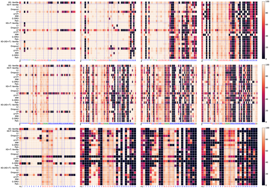
Figure 1: Average and individual pass rates for all tasks, methods and training configurations. From first to third row: results for SENT, PARA and READ. From first to fourth column: seen evaluation, functionality generalisation, functionality class generalisation, and test type generalisation scores. The y-axis correspond to all training configuration-method pairs; the x-axis shows the average functionality pass rate followed by the individual pass rates. The blue horizontal and vertical lines demarcate different training configurations and functionality classes, respectively. The colors in the x-axis designate the different test types: blue for MFTs, red for INVs an green for DIRs.

5.1 I.i.d. and generalisation scores

Table 3 exhibits i.i.d. and aggregate $\text{G}_{\text{}}$ scores for all tasks, training configurations and generalisation methods. Figure 1 presents pass rates of individual functionalities.

Seen performance:  Fine-tuning on test suite data led to improvements for all tasks: the $\text{G}_{\text{seen}}$ scores are generally higher than the baseline scores (first row in Table 3).

That is, models were able to generalise across test cases from covered functionalities (from $\mathcal{T}_{\text{train}}$ to $\mathcal{T}_{\text{test}}$) while retaining reasonable i.i.d. data performance. In some specific training configuration-method combinations this was not the case. We discuss this below when we compare methods and report the degenerate solutions.

Generalisation performance:  For any given configuration-method pair, $\text{G}_{\text{seen}}$ is higher than $\text{G}_{\text{func}}$, $\text{G}_{\text{class}}$ and $\text{G}_{\text{type}}$, indicating a generalisation gap between seen and unseen functionalities. Furthermore, for all tasks, average (across methods) $\text{G}_{\text{func}}$ is higher than average $\text{G}_{\text{class}}$, which is higher than average $\text{G}_{\text{type}}$, indicating that generalisation gets harder as one moves from unseen functionalities to unseen functionality classes and test types. This aligns with previous work Luz de Araujo and Roth (2022), in which hate speech detection models are found to generalise within—but not across—functionality classes.

Improvements over the IID baseline were task dependent. Almost all configuration-method pairs achieved $\text{G}_{\text{func}}$ (22 of 24) and $\text{G}_{\text{class}}$ (20 of 24) scores significantly higher that the IID baseline for SENT, with improvements over the baseline as high as 18.44 and 12.84 percentage points (p.p.) for each metric, respectively. For PARA, improving over $\text{G}_{\text{class}}$ proved much harder—only seven configuration-method pairs could do so. Increases in score were also less pronounced, the best $\text{G}_{\text{func}}$ and $\text{G}_{\text{class}}$ scores being 6.91 and 2.19 p.p. above the baseline. READ was the one with both rarer and subtler improvements, with a third of the approaches significantly improving functionality and none significantly improving functionality class generalisation. Improvements in each case were as high as 4.70 and 0.51 p.p. over the baseline.

I.i.d. performance:  Fine-tuning on test suite data only (IID$\rightarrow$T configuration) reduced performance for all tasks’ i.i.d. test sets. Fine-tuning on both suite and i.i.d. examples (IID$+$T and IID$\rightarrow$(IID$+$T)) helped retain—or improve—performance in some cases, but decreases were still more common. The IID$\rightarrow$(IID$+$T) configuration was the most robust regarding i.i.d. scores, with an average change (compared to the IID baseline) of $-1.43$/$-0.50$/$-1.73$ for SENT/PARA/READ.

5.2 Training configuration and method comparison

Using a mixture of i.i.d. and suite samples proved essential to retain i.i.d. performance: the overall scores (average over methods and i.i.d. test sets) for each configuration are 67.52, 76.33 and 87.98 for IID$\rightarrow$T, IID$+$T, and IID$\rightarrow$(IID$+$T) respectively.

That said, the environment-based generalisation algorithms (IRM, DRO and Fish) struggled in the IID$+$T configuration, underperforming when compared with the other methods. We hypothesize that in these scenarios models simply do not see enough i.i.d. data, as we treat it as just one more environment among many others (reaching as much as 54 in PARA). LP also achieves subpar scores, even though i.i.d. data is not undersampled. The problem here is the frozen feature encoder, as BERT features are not good enough without fine-tuning on i.i.d. task data—as was done in the other configurations, with clear benefits for LP.

No individual method performed best for all scores and tasks. That said, IID$\rightarrow$(IID$+$T) with L2, LP, LP-FT or Fish was able to achieve $\text{G}_{\text{func}}$ and $\text{G}_{\text{class}}$ scores higher or not significantly different from the baseline in all tasks, though IID$\rightarrow$(IID$+$T) with dropout was the best when score is averaged over all tasks and generalisation measures. Considering this same metric, IID$\rightarrow$(IID$+$T) was the most consistently good configuration, with all methods improving over the average IID baseline.

5.3 DIR applicability

We have found that DIRs, as used for SENT, have limited applicability for both testing and training. The reason for that is that models are generally very confident about their predictions: the average prediction confidence for the test suite predictions is $0.97$ for the IID model. On the evaluation side, this makes some DIRs impossible to fail: the confidence cannot get higher and fail “not more confident” expectations. On the training side, DIRs do not add much of a training signal, as the training loss is near zero from the very beginning.

We see an additional problem with DIRs in the SENT setting: they confuse prediction confidence with sentiment intensity. Though prediction confidence may correlate with sentiment intensity, uncertainty also signals difficulty and ambiguousness Swayamdipta et al. (2020). Consequently, sentiment intensity tests may not be measuring the intended phenomena. One alternative would be to disentangle the two factors: using prediction values only for confidence-based tests, and sentiment intensity tests only for sentiment analysis tasks with numeric or fine-grained labels.

5.4 Negative transfer

Though $\text{G}_{\text{class}}$ scores are generally lower than $\text{G}_{\text{func}}$ scores, this is not always the case for the pass rates of individual functionalities. When there are contrastive functionalities within a class—those whose test cases have similar surface form but entirely different expected behaviours—it is very difficult to generalise from one to the other.

For example, the SRL class in PARA contains the functionalities “order does not matter for symmetric relations” and “order does matter for asymmetric relations” (functionalities 41 and 42 in the second row of Fig. 1). Their test cases are generated by nearly identical templates where the only change is the relation placeholder. Examples from the first and second functionalities would include (Q1: Is Natalie dating Sophia? Q2: Is Sophia dating Natalie?) and (Q1: Is Matthew lying to Nicole? Q2: Is Nicole lying to Matthew?) respectively. Though their surface forms are similar, they have opposite labels: duplicate and not duplicate.

To compute $s_{\mathcal{T}\text{func}}$, a model is trained with samples from one functionality and evaluated on samples from the other. Consequently, the surface form will be spuriously correlated with the label seen during training and models may blindly assign it to the question pairs that fit the template. This would work well for the seen functionality, but samples from the unseen one would be entirely misclassified. Conversely, when computing the $s_{\mathcal{T}\text{class}}$ score, the model will not have been trained on either of the functionalities and will not have the chance to adopt the heuristic, leading to better unseen pass rates.

5.5 Degenerate solutions

Settings where the $\text{G}_{\text{type}}$ score is higher than the baseline are much rarer than for the other measures, happening only in one case for SENT (IID$\rightarrow$T with dropout) and never for READ. One explanation is that training only on perturbation-based tests (with no MFTs) can lead to degenerate solutions, such as passing all tests by always predicting the same class.

To assess if that was the case, we examined the predictions on the SST-2 test set of the IID$\rightarrow$T vanilla model fine-tuned only on DIRs and INVs. We have found that $95.18\%$ of the i.i.d. data points were predicted as negative, though the ground truth frequency for that label is $47.25\%$. When examining the predictions for MFTs, the results are even more contrasting: $0.29\%$ of the predictions were negative, with the ground truth frequency being $43.42\%$. These results show that the model has, indeed, adopted the degenerate solution. Interestingly, it predicts different classes depending on the domain, almost always predicting negative for i.i.d. data and positive for suite data.

The gap between $\text{G}_{\text{class}}$ and $\text{G}_{\text{type}}$ scores in PARA is not as severe, possibly due to the supervised signal in its DIRs. Since these tests expect inputs to correspond to specific labels—as opposed to DIRs for SENT, which check for changes in prediction confidence—always predicting the same class would not be a good solution. Indeed, when examining the predictions on the QQP test set of the vanilla IID$\rightarrow$T model fine-tuned with no MFT data, we see that $58.70\%$ of question pairs are predicted as not duplicate, which is similar to the ground truth frequency, $63.25\%$. The same is true when checking the predictions for MFTs: $64.47\%$ of the data points are predicted as not duplicate, against a ground truth frequency of $52.46\%$.

The READ scenario is more complex—instead of categories, spans are extracted. Manual inspection showed that some IID$\rightarrow$T models adopted degenerate solutions (e.g.  extracting the first word, a full stop or the empty span as the answer), even when constrained by the MFT supervised signal. Interestingly, the degenerate solutions were applied only for INV tests (where such invariant predictions work reasonably) and i.i.d. examples (where they do not). On the other hand, these models were able to handle the MFTs well, obtaining near perfect scores and achieving high $s_{\mathcal{T}\text{seen}}$ scores even though i.i.d. performance is catastrophic. The first grid of the third row in Fig. 1 illustrates this: the high $s_{\mathcal{T}\text{seen}}$ scores are shown on the first column, and the MFT pass rates on the columns with blue x-axis numbers.

5.6 Summary interpretation of the results

Figure 1

Figure 1 supports fine-grained analyses that consider performance on individual functionalities in each generalisation scenario. One can interpret it horizontally to assess the functionality pass rates for a particular method. For example, the bottom left grid, representing seen results for READ, shows that IID$+$T with LP behaves poorly on almost all functionalities, confirming the importance of fine-tuning BERT pre-trained features (§ 5.2).

Alternatively, one can interpret it vertically to assess performance and generalisation trends for individual functionalities. For example, models generalised well to functionality 21 of the READ suite (second grid of the bottom row), with most methods improving over the IID baseline. However, under the functionality class evaluation scenario (third grid of the bottom row), improvements for functionality 21 are much rarer. That is, the models were able to generalise to functionality 21 as long as they were fine-tuned on cases from functionalities from the same class (20 and 22).

Such fine-grained analyses show the way for more targeted explorations of generalisation (e.g. why do models generalise to functionality 21 but not to functionality 20?), which can guide subsequent data annotation, selection and creation efforts, and shed light on model limitations.

Table 3

For i.i.d. results, we refer to the SST2, QQP and SQuAD columns. These show that the suite-augmented configuration and methods (all rows below and including IID$\rightarrow$T Vanilla) generally hurt i.i.d. performance. However, improvements can be found for some methods in the IID$+$T and IID$\rightarrow$(IID$+$T). Takeaway: fine-tuning on behavioural tests degrades model general performance, which can be mitigated by jointly fine-tuning on i.i.d. samples and behavioural tests.

For performance concerning seen functionalities, we refer to the $\text{G}_{\text{seen}}$ columns. Generalisation scores concerning unseen functionalities, functionality classes and test types can be found in the $\text{G}_{\text{func}}$, $\text{G}_{\text{class}}$ and $\text{G}_{\text{type}}$ columns. Across all tasks, training configurations and methods, the $\text{G}_{\text{seen}}$ scores are higher than the others. Takeaway: evaluating only on the seen functionalities Liu et al. (2019); Malon et al. (2022) is overoptimistic—improving performance on seen cases may come at the expense of degradation on unseen cases. This is detected by the underperforming generalisation scores.

Previous work on generalisation in behavioural learning Luz de Araujo and Roth (2022); Rozen et al. (2019) corresponds to the IID$\rightarrow$T Vanilla row. It shows deterioration of i.i.d. scores, poor generalisation in some cases, and lower average performance compared with the IID baseline. However, our experiments with additional methods (all rows below IID$\rightarrow$T Vanilla), show that some configuration-method combinations improve the average performance. Takeaway: while naive behavioural learning generalises poorly, more sophisticated algorithms can lead to improvements. BeLUGA is a method that detects and measures further algorithmic improvements.

6 Related work

Traditional NLP benchmarks Wang et al. (2018, 2019) are composed of text corpora that reflect the naturally-occurring language distribution, which may fail to sufficiently capture rarer, but important phenomena Belinkov and Glass (2019). Moreover, since these benchmarks are commonly split into identically distributed train and test sets, spurious correlations in the former will generally hold for the latter. This may lead to the obfuscation of unintended behaviours, such as the adoption of heuristics that work well for the data distribution but not in general Linzen (2020); McCoy et al. (2019). To account for these shortcomings, complementary evaluations methods have been proposed, such as using dynamic benchmarks Kiela et al. (2021) and behavioural test suites Kirk et al. (2022); Röttger et al. (2021); Ribeiro et al. (2020).

A line of work has explored how training on challenge and test suite data affects model performance by fine-tuning on examples from specific linguistic phenomena and evaluating on other samples from the same phenomena Malon et al. (2022); Liu et al. (2019). This is equivalent to our seen evaluation scenario, and thus cannot distinguish between models with good generalisation and those that have overfitted to the seen phenomena. We account for that with our additional generalisation measures, computed using only data from held-out phenomena.

Other efforts have also used controlled data splits to examine generalisation: McCoy et al. (2019) have trained and evaluated on data from disjoints sets of phenomena relevant for Natural Language Inference (NLI); Rozen et al. (2019) have split challenge data according to sentence length and constituency parsing tree depth, creating a distribution shift between training and evaluation data; Luz de Araujo and Roth (2022) employ a cross-functional analysis of generalisation in hate speech detection. Though these works address the issue of overfitting to seen phenomena, their analyses are restricted to specific tasks and training configurations. Our work gives a more comprehensive view of generalisation of behavioural learning by examining different tasks, training configurations, test types and metrics. Additionally, we use this setting as an opportunity to compare generalisation impact of both simple regularisation mechanisms and state-of-the-art domain generalisation algorithms.

7 Conclusion

We have presented BeLUGA, a framework for cross-functional analysis of generalisation in NLP systems that both makes explicit the desired system traits and allows for quantifying and examining several axes of generalisation. While in this work we have used BeLUGA to analyse data from behavioural suites, it can be applied in any setting where one has access to data structured into meaningful groups (e.g. demographic data, linguistic phenomena, domains).

We have shown that, while model performance for seen phenomena greatly improves after fine-tuning on test suite data, the generalisation scores reveal a more nuanced view, in which the actual benefit is less pronounced and depends on the task and training configuration-method combination. We have found the IID$\rightarrow$(IID$+$T) configuration to result in the most consistent improvements. Conversely, some methods struggle in the IID$\rightarrow$T and IID$+$T settings by overfitting to the suite or underfitting i.i.d. data, respectively. In these cases, a model both practically aces all tests and fails badly for i.i.d. data, which reinforces the importance of considering both i.i.d. and test suite performance when comparing systems, which is accounted for by BeLUGA’s aggregate scores.

These results show that naive behavioural learning has unintended consequences, which the IID$\rightarrow$(IID$+$T) configuration mitigates to some degree. There is still much room for improvement, though, especially if generalisation to unseen types of behaviour is desired. Through BeLUGA, progress in that direction is measurable, and further algorithmic improvements might make behavioural learning an option to ensure desirable behaviours and preserve general performance and generalisability of the resulting models. We do not recommend training on behavioural tests in the current technological state. Instead, we show a way to improve research on reconciling the qualitative guidance of behavioural tests with desired generalisation in NLP models.

References

- Arjovsky et al. (2019) Martín Arjovsky, Léon Bottou, Ishaan Gulrajani, and David Lopez-Paz. 2019. Invariant risk minimization. CoRR, abs/1907.02893v3.
- Belinkov and Glass (2019) Yonatan Belinkov and James Glass. 2019. Analysis methods in neural language processing: A survey. Transactions of the Association for Computational Linguistics, 7:49–72.
- Devlin et al. (2019) Jacob Devlin, Ming-Wei Chang, Kenton Lee, and Kristina Toutanova. 2019. BERT: Pre-training of deep bidirectional transformers for language understanding. In Proceedings of the 2019 Conference of the North American Chapter of the Association for Computational Linguistics: Human Language Technologies, Volume 1 (Long and Short Papers), pages 4171–4186, Minneapolis, Minnesota. Association for Computational Linguistics.
- Dranker et al. (2021) Yana Dranker, He He, and Yonatan Belinkov. 2021. IRM—when it works and when it doesn't: A test case of natural language inference. In Advances in Neural Information Processing Systems, volume 34, pages 18212–18224. Curran Associates, Inc.
- Iyer et al. (2017) Shankar Iyer, Nikhil Dandekar, and Kornél Csernai. 2017. First quora dataset release: Question pairs. Available online at https://quoradata.quora.com/First-Quora-Dataset-Release-Question-Pairs.
- Kiela et al. (2021) Douwe Kiela, Max Bartolo, Yixin Nie, Divyansh Kaushik, Atticus Geiger, Zhengxuan Wu, Bertie Vidgen, Grusha Prasad, Amanpreet Singh, Pratik Ringshia, Zhiyi Ma, Tristan Thrush, Sebastian Riedel, Zeerak Waseem, Pontus Stenetorp, Robin Jia, Mohit Bansal, Christopher Potts, and Adina Williams. 2021. Dynabench: Rethinking benchmarking in NLP. In Proceedings of the 2021 Conference of the North American Chapter of the Association for Computational Linguistics: Human Language Technologies, pages 4110–4124, Online. Association for Computational Linguistics.
- Kirk et al. (2022) Hannah Kirk, Bertie Vidgen, Paul Rottger, Tristan Thrush, and Scott Hale. 2022. Hatemoji: A test suite and adversarially-generated dataset for benchmarking and detecting emoji-based hate. In Proceedings of the 2022 Conference of the North American Chapter of the Association for Computational Linguistics: Human Language Technologies, pages 1352–1368, Seattle, United States. Association for Computational Linguistics.
- Kumar et al. (2022) Ananya Kumar, Aditi Raghunathan, Robbie Matthew Jones, Tengyu Ma, and Percy Liang. 2022. Fine-tuning can distort pretrained features and underperform out-of-distribution. In Proceedings of the 10th International Conference on Learning Representations, Online. OpenReview.net.
- Linzen (2020) Tal Linzen. 2020. How can we accelerate progress towards human-like linguistic generalization? In Proceedings of the 58th Annual Meeting of the Association for Computational Linguistics, pages 5210–5217, Online. Association for Computational Linguistics.
- Liu et al. (2019) Nelson F. Liu, Roy Schwartz, and Noah A. Smith. 2019. Inoculation by fine-tuning: A method for analyzing challenge datasets. In Proceedings of the 2019 Conference of the North American Chapter of the Association for Computational Linguistics: Human Language Technologies, Volume 1 (Long and Short Papers), pages 2171–2179, Minneapolis, Minnesota. Association for Computational Linguistics.
- Loshchilov and Hutter (2019) Ilya Loshchilov and Frank Hutter. 2019. Decoupled weight decay regularization. In Proceedings of the 7th International Conference on Learning Representations, New Orleans, LA, USA. OpenReview.net.
- Luz de Araujo and Roth (2022) Pedro Henrique Luz de Araujo and Benjamin Roth. 2022. Checking HateCheck: a cross-functional analysis of behaviour-aware learning for hate speech detection. In Proceedings of NLP Power! The First Workshop on Efficient Benchmarking in NLP, pages 75–83, Dublin, Ireland. Association for Computational Linguistics.
- Ma et al. (2021) Zhiyi Ma, Kawin Ethayarajh, Tristan Thrush, Somya Jain, Ledell Wu, Robin Jia, Christopher Potts, Adina Williams, and Douwe Kiela. 2021. Dynaboard: An evaluation-as-a-service platform for holistic next-generation benchmarking. In Advances in Neural Information Processing Systems, volume 34, pages 10351–10367. Curran Associates, Inc.
- Malon et al. (2022) Christopher Malon, Kai Li, and Erik Kruus. 2022. Fast few-shot debugging for NLU test suites. In Proceedings of Deep Learning Inside Out (DeeLIO 2022): The 3rd Workshop on Knowledge Extraction and Integration for Deep Learning Architectures, pages 79–86, Dublin, Ireland and Online. Association for Computational Linguistics.
- McCoy et al. (2019) Tom McCoy, Ellie Pavlick, and Tal Linzen. 2019. Right for the wrong reasons: Diagnosing syntactic heuristics in natural language inference. In Proceedings of the 57th Annual Meeting of the Association for Computational Linguistics, pages 3428–3448, Florence, Italy. Association for Computational Linguistics.
- Niven and Kao (2019) Timothy Niven and Hung-Yu Kao. 2019. Probing neural network comprehension of natural language arguments. In Proceedings of the 57th Annual Meeting of the Association for Computational Linguistics, pages 4658–4664, Florence, Italy. Association for Computational Linguistics.
- Rajpurkar et al. (2016) Pranav Rajpurkar, Jian Zhang, Konstantin Lopyrev, and Percy Liang. 2016. SQuAD: 100,000+ questions for machine comprehension of text. In Proceedings of the 2016 Conference on Empirical Methods in Natural Language Processing, pages 2383–2392, Austin, Texas. Association for Computational Linguistics.
- Ribeiro et al. (2020) Marco Tulio Ribeiro, Tongshuang Wu, Carlos Guestrin, and Sameer Singh. 2020. Beyond accuracy: Behavioral testing of NLP models with CheckList. In Proceedings of the 58th Annual Meeting of the Association for Computational Linguistics, pages 4902–4912, Online. Association for Computational Linguistics.
- Röttger et al. (2021) Paul Röttger, Bertie Vidgen, Dong Nguyen, Zeerak Waseem, Helen Margetts, and Janet Pierrehumbert. 2021. HateCheck: Functional tests for hate speech detection models. In Proceedings of the 59th Annual Meeting of the Association for Computational Linguistics and the 11th International Joint Conference on Natural Language Processing (Volume 1: Long Papers), pages 41–58, Online. Association for Computational Linguistics.
- Rozen et al. (2019) Ohad Rozen, Vered Shwartz, Roee Aharoni, and Ido Dagan. 2019. Diversify your datasets: Analyzing generalization via controlled variance in adversarial datasets. In Proceedings of the 23rd Conference on Computational Natural Language Learning (CoNLL), pages 196–205, Hong Kong, China. Association for Computational Linguistics.
- Sagawa et al. (2020) Shiori Sagawa, Pang Wei Koh, Tatsunori B. Hashimoto, and Percy Liang. 2020. Distributionally robust neural networks for group shifts: On the importance of regularization for worst-case generalization. In Proceedings of the 8th International Conference on Learning Representations, Addis Ababa, Ethiopia. OpenReview.net.
- Shi et al. (2022) Yuge Shi, Jeffrey Seely, Philip H. S. Torr, N. Siddharth, Awni Hannun, Nicolas Usunier, and Gabriel Synnaeve. 2022. Gradient matching for domain generalization. In Proceedings of the 10th International Conference on Learning Representations, Virtual. OpenReview.net.
- Socher et al. (2013) Richard Socher, Alex Perelygin, Jean Wu, Jason Chuang, Christopher D. Manning, Andrew Ng, and Christopher Potts. 2013. Recursive deep models for semantic compositionality over a sentiment treebank. In Proceedings of the 2013 Conference on Empirical Methods in Natural Language Processing, pages 1631–1642, Seattle, Washington, USA. Association for Computational Linguistics.
- Swayamdipta et al. (2020) Swabha Swayamdipta, Roy Schwartz, Nicholas Lourie, Yizhong Wang, Hannaneh Hajishirzi, Noah A. Smith, and Yejin Choi. 2020. Dataset cartography: Mapping and diagnosing datasets with training dynamics. In Proceedings of the 2020 Conference on Empirical Methods in Natural Language Processing (EMNLP), pages 9275–9293, Online. Association for Computational Linguistics.
- Wang et al. (2019) Alex Wang, Yada Pruksachatkun, Nikita Nangia, Amanpreet Singh, Julian Michael, Felix Hill, Omer Levy, and Samuel Bowman. 2019. Superglue: A stickier benchmark for general-purpose language understanding systems. In Advances in Neural Information Processing Systems, volume 32. Curran Associates, Inc.
- Wang et al. (2018) Alex Wang, Amanpreet Singh, Julian Michael, Felix Hill, Omer Levy, and Samuel Bowman. 2018. GLUE: A multi-task benchmark and analysis platform for natural language understanding. In Proceedings of the 2018 EMNLP Workshop BlackboxNLP: Analyzing and Interpreting Neural Networks for NLP, pages 353–355, Brussels, Belgium. Association for Computational Linguistics.
- Wu et al. (2019) Tongshuang Wu, Marco Tulio Ribeiro, Jeffrey Heer, and Daniel Weld. 2019. Errudite: Scalable, reproducible, and testable error analysis. In Proceedings of the 57th Annual Meeting of the Association for Computational Linguistics, pages 747–763, Florence, Italy. Association for Computational Linguistics.
- Yeh (2000) Alexander Yeh. 2000. More accurate tests for the statistical significance of result differences. In COLING 2000 Volume 2: The 18th International Conference on Computational Linguistics.
- Yu et al. (2021) Yue Yu, Simiao Zuo, Haoming Jiang, Wendi Ren, Tuo Zhao, and Chao Zhang. 2021. Fine-tuning pre-trained language model with weak supervision: A contrastive-regularized self-training approach. In Proceedings of the 2021 Conference of the North American Chapter of the Association for Computational Linguistics: Human Language Technologies, pages 1063–1077, Online. Association for Computational Linguistics.
- Zellers et al. (2019) Rowan Zellers, Ari Holtzman, Yonatan Bisk, Ali Farhadi, and Yejin Choi. 2019. HellaSwag: Can a machine really finish your sentence? In Proceedings of the 57th Annual Meeting of the Association for Computational Linguistics, pages 4791–4800, Florence, Italy. Association for Computational Linguistics.