On the Correspondence between Compositionality and Imitation in Emergent Neural Communication
Abstract
Compositionality is a hallmark of human language that not only enables linguistic generalization, but also potentially facilitates acquisition. When simulating language emergence with neural networks, compositionality has been shown to improve communication performance; however, its impact on imitation learning has yet to be investigated. Our work explores the link between compositionality and imitation in a Lewis game played by deep neural agents. Our contributions are twofold: first, we show that the learning algorithm used to imitate is crucial: supervised learning tends to produce more average languages, while reinforcement learning introduces a selection pressure toward more compositional languages. Second, our study reveals that compositional languages are easier to imitate, which may induce the pressure toward compositional languages in RL imitation settings.
1 Introduction
Compositionality, a key feature of human language, makes it possible to derive the meaning of a complex expression from the combination of its constituents (Szabo, 2020). It has been suggested that more compositional languages are easier to acquire for both humans and artificial agents Raviv et al. (2021); Li and Bowling (2019); Ren et al. (2020); Chaabouni et al. (2020). Therefore, to better understand the factors underlying language transmission, it is crucial to understand the relationship between ease-of-acquisition and compositionality.
We study the link between compositionality and ease-of-acquisition in the context of emergent communication. In this setting, two deep artificial agents with asymmetric information, a Sender and a Receiver, must develop communication from scratch in order to succeed at a cooperative game (Havrylov and Titov, 2017; Lazaridou et al., 2017; Lazaridou and Baroni, 2020). We will refer to this mode of language learning, in which agents develop language via feedback from mutual interaction, as communication-based learning.
Several studies have linked compositionality to ease-of-acquisition in communication-based learning. Chaabouni et al., 2020 show compositionality predicts efficient linguistic transmission from Senders to new Receivers. Conversely, Li and Bowling, 2019 re-pair a Sender periodically with new Receivers, and show this ease-of-teaching pressure improves compositionality.
Communication-based learning is not the only possibility for language learning, however. Humans also crucially acquire language through imitation-based learning, in which they learn by observing other humans’ language use (Kymissis and Poulson, 1990). Ren et al., 2020 and Chaabouni et al., 2020 employ imitation learning, where in the first study, agents undergo a supervised imitation stage before communication-based learning, and where in the second, agents alternate between communication-based learning and imitating the best Sender. However, the dynamics of imitation are not the focus in either study. For such an important vehicle of language acquisition, imitation-based learning thus remains under-explored in the emergent communication literature.
We extend these lines of inquiry to systematically investigate compositionality in imitation-based learning.111…for artificial agents. We do not test theories of human imitation learning. Our contributions are as follows: (1) We show that imitation can automatically select for compositional languages under a reinforcement learning objective; and (2) that this is likely due to ease-of-learning of compositional languages.
2 Setup
We study imitation in the context of referential communication games (Lewis, 1969). In this setting, a Sender agent observes an object and transmits a message to a second Receiver agent. Using this message, the Receiver performs an action for which both agents receive a reward. Over the course of the game, agents converge to a referential system , which we refer to as an emergent language.
Measuring Compositionality
Evaluating compositionality in emergent languages is not straightforward given their grammars are a-priori unknown. Therefore, we quantify compositionality using topographic similarity (topsim) Kirby and Brighton (2006), a grammar-agnostic metric widely applied to emergent languages in the literature. Topsim is defined as the Spearman correlation between Euclidean distances in the input space and Levenstein distances in the message space– that is, it captures the intuition that nearby inputs should be described with similar messages. While we consider other compositionality metrics such as positional disentanglement Chaabouni et al. (2020), we focus on topsim due to its high correlation with generalization accuracy () (Rita et al., 2022b). See section A.3 for extended experiments on compositionality metrics and generalization.
2.1 Imitation Task
To investigate whether compositional languages are selected for in imitation, we posit an imitation task where one new Imitator Sender or Receiver simultaneously imitates several Expert Senders or Receivers with varying topsims. Both Sender and Receiver agents are parameterized by single-layer GRUs Cho et al. (2014) that are deterministic after training (see appendix B for implementation).222Experiments are implemented using EGG Kharitonov et al. (2021). Code may be found at
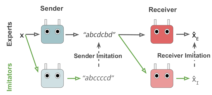
https://github.com/chengemily/EGG/tree/imitation. While we explore imitation for both agents, we focus on Sender imitation in the main text, and extend to Receiver imitation in appendix E. A minimal example of imitation learning with only one Expert Sender-Receiver pair is shown in fig. 1.
The Sender imitation task is as follows: given a set of Expert Senders, we train an identical, newly initialized Sender on the Experts’ inputs and outputs . That is, for each round of training, all Experts as well as the Imitator Sender receive input and output and , respectively. The Imitator is then tasked to minimize the difference between their output and a uniform mixture of the Expert outputs.
Dataset
Data in the imitation task consists of inputs and outputs of pairs of Expert agents trained to convergence on a communication game– in our case, the two-agent reconstruction task of Kottur et al. (2017). To generate the Experts, we pre-train Sender-Receiver pairs on this reconstruction task to high validation accuracy () (task and training details in appendix A).
Expert training produces the following data: 1) inputs ; 2) messages corresponding to Expert Senders’ encodings of ; and 3) outputs , the Expert Receivers’ reconstructions of given .
Each input denotes an object in an “attribute-value world", where the object has attributes, and each attribute takes possible values. We represent by a concatenation of one-hot vectors, each of dimension . On the other hand, messages are discrete sequences of fixed length , consisting of symbols taken from a vocabulary . We set , , , and , corresponding to a relatively large attribute-value setting in the literature (Table 1 of Galke et al. (2022)).
We split the input data () into a training set and two holdout sets. Similar to Chaabouni et al. (2020), we define two types of holdouts: a zero-shot generalization set (), where one value is held-out during training, and an in-distribution generalization set (). The training set, on which we both train and validate, represents 1% of in-distribution data (). These data splits are used in Expert training and are inherited by the imitation task (see section B.2 for details on generating the data split).
Imitation learning algorithms
While imitation is classically implemented as supervised learning, we test two imitation learning procedures: 1) supervised learning (SV) with respect to the cross-entropy loss between Imitator and Expert outputs; and 2) reinforcement learning with the REINFORCE algorithm (RF) Williams (1992), using per-symbol accuracy as a reward. When using REINFORCE, we additionally include an entropy regularization term weighted by to encourage exploration, and subtract a running mean baseline from the reward to improve training stability (Williams and Peng, 1991). See appendix D for loss functions and B.2 for detailed hyperparameter settings.
2.2 Evaluation
To evaluate properties of imitation learning, we identify three descriptors of interest: validation accuracy, ease-of-imitation, and selection of compositional languages.
Accuracy
We evaluate imitation performance between an Imitator and Expert by the average per-symbol accuracy between their messages given an input. When using REINFORCE, training accuracy is computed using the Imitators’ sampled output while validation accuracy is computed using the Imitators’ argmax-ed output.
Ease-of-imitation
We evaluate ease-of-imitation of a language two ways. First, imitation sample complexity (): the number of epochs needed to reach 99% validation accuracy, and second, imitation speed-of-learning (): the area under the validation accuracy curve, cut-off at epochs chosen by visual inspection of convergence.
Selection of compositional languages
Sender imitation consists of learning one-to-one input-to-message mappings from a sea of one-to-many Expert mappings. Then, the Imitator’s language will consist of a mixture of Expert languages, where the mixture weights reveal the extent of selection.
In this mixture, we proxy the Imitator’s learned weight for an Expert as the proportion of messages in the training set for which Imitator accuracy on the Expert message is the highest. Note that the coefficients may not add to one: if the highest Expert accuracy for a message does not exceed chance (10%), we consider the message unmatched.
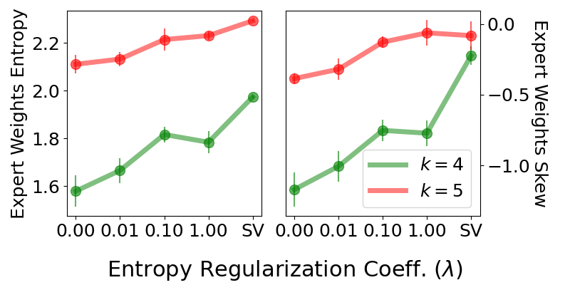
To quantify selection, we use the intuition that selection corresponds jointly to peakedness and asymmetry in the learned distribution over Expert languages sorted by topsim. We evaluate peakedness using the Shannon entropy and asymmetry using Fisher’s moment coefficient of skew of Expert weights. Formally, let there be Experts, where Experts are sorted in ascending order of topsim (Expert =1 is the least and = is the most compositional, respectively). The Imitator learns a mixture of the Expert languages with weights (normalized). Given , we evaluate peakedness with:
| (1) |
To quantify asymmetry of expert weights, we estimate the Fisher’s moment coefficient of skew:
| (2) |
where is the mean and is the standard deviation of . A skew of 0 implies perfect symmetry, positive skew corresponds to a right-tailed distribution, and negative skew corresponds to a left-tailed distribution. Intuitively, the more negative the skew of the Expert weights, the more weight lies on the right side of the distribution, hence the greater “compositional selection effect".
We proxy selection, then, by a negative skew (more weight assigned to high-topsim Experts) and low entropy (peakedness) in the Expert weight distribution.
3 Imitation and Selection of Compositionality
We present results for imitation on mixtures of - Expert Senders. First, we generate 30 Expert languages from the referential task, initially considering Expert distributions corresponding to evenly-spaced percentiles of topsim, including the minimum and maximum . For example, when , we take the lowest, percentile, and highest-topsim languages. All results are aggregated over random seeds after training epochs.
We find that (1) whether Imitators prefer compositional Experts depends crucially on the learning algorithm: imitation by reinforcement results in marked compositional selection compared to supervision; and (2) compositional selection also depends on variance of expert topsims, entropy regularization coefficient, and number of Experts.
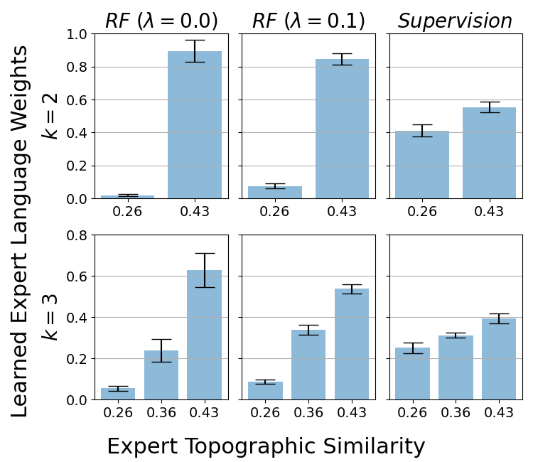
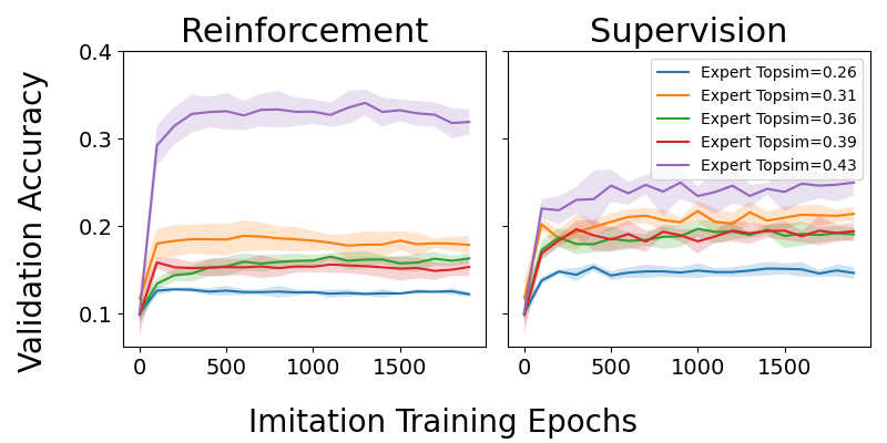
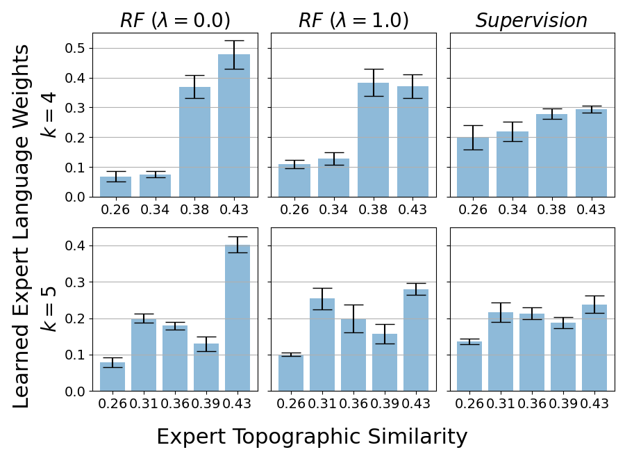
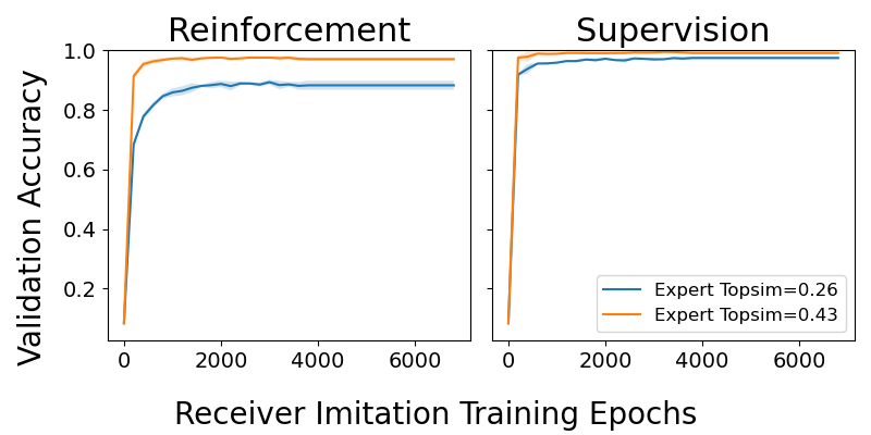
The distribution of learned Expert weights in fig. 2, as well as imitation validation accuracy curves in fig. C.2, evidence that in imitation by supervision, the empirical mixture is closer to uniform than when imitating by reinforcement. Otherwise, when optimizing using reinforcement, the Imitator selects more compositional languages.
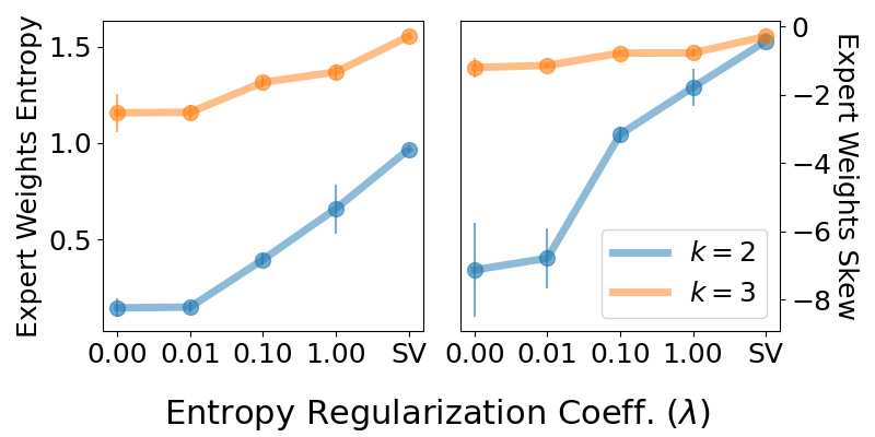
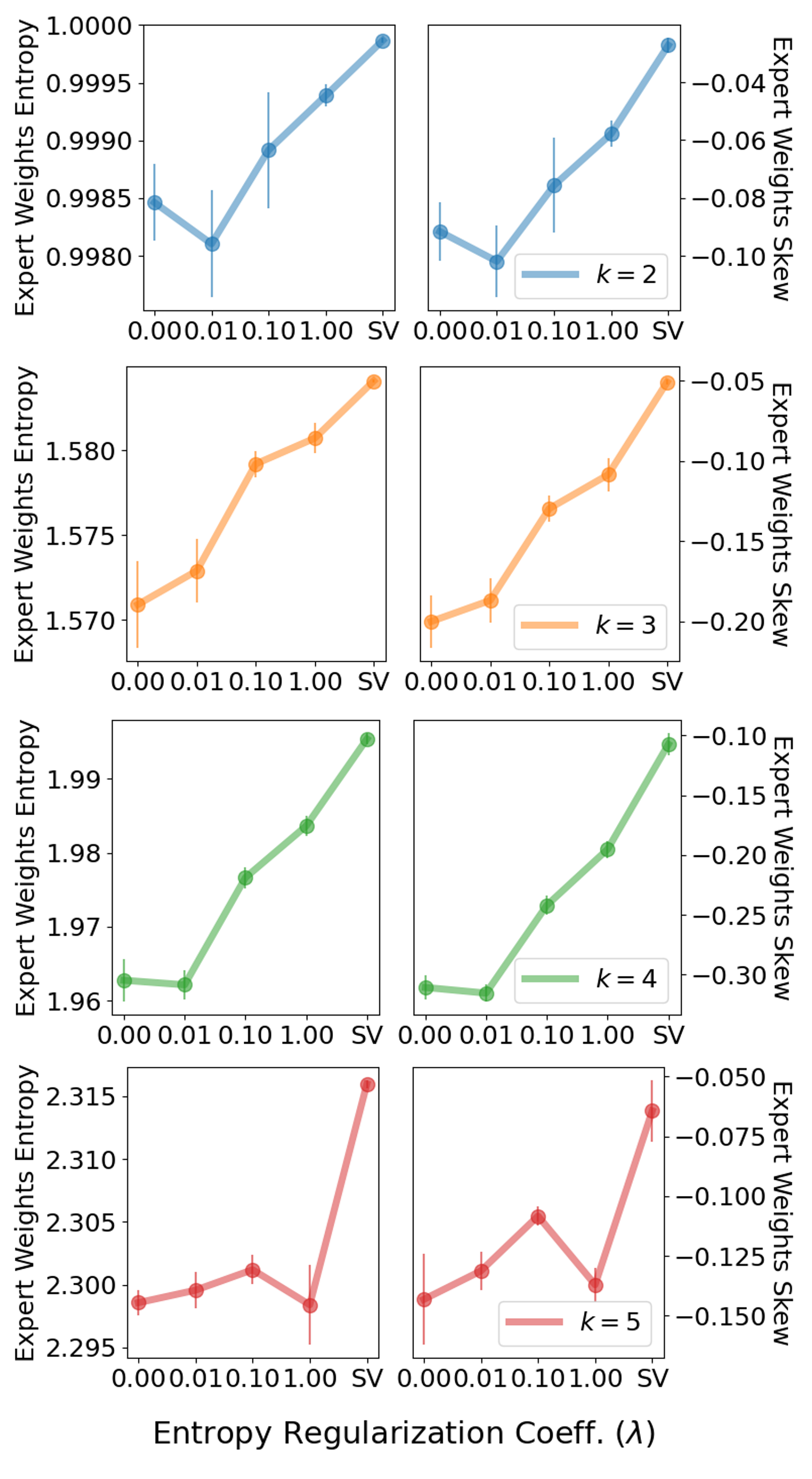
The shape of the Expert weight distribution is tempered by the entropy regularization coefficient : smaller results in greater compositional selection (that is, lower entropy and more negative skew) of the weight distribution (fig. 3). At the limit, imitation by supervision results in the highest entropy and the skew that is closest to zero.
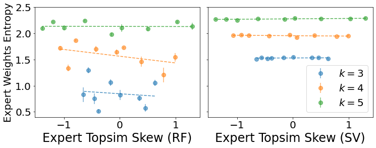
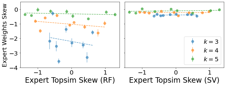
We then test the effect of Expert topsim distribution asymmetry on the learned weights. To do so, for each , we generate Expert topsim distributions with varying skew, following the procedure outlined in section D.2 (when , skew is mechanically ). We find that for both REINFORCE and supervision, holding equal, the skew and entropy of the learned Expert weight distribution are robust (i.e., not correlated) to the skew of the underlying Expert topsim distribution (fig. D.2). This is desirable when imitating by reinforcement and undesirable when imitating by supervision: for example, consider Expert topsim distributions [low high high] (skew) and [low low high] (skew). In both cases, REINFORCE will select a high-topsim Expert, and supervision will weight all Experts equally, that is, supervision is unable to de-select poor topsims.
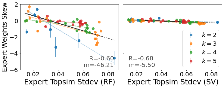
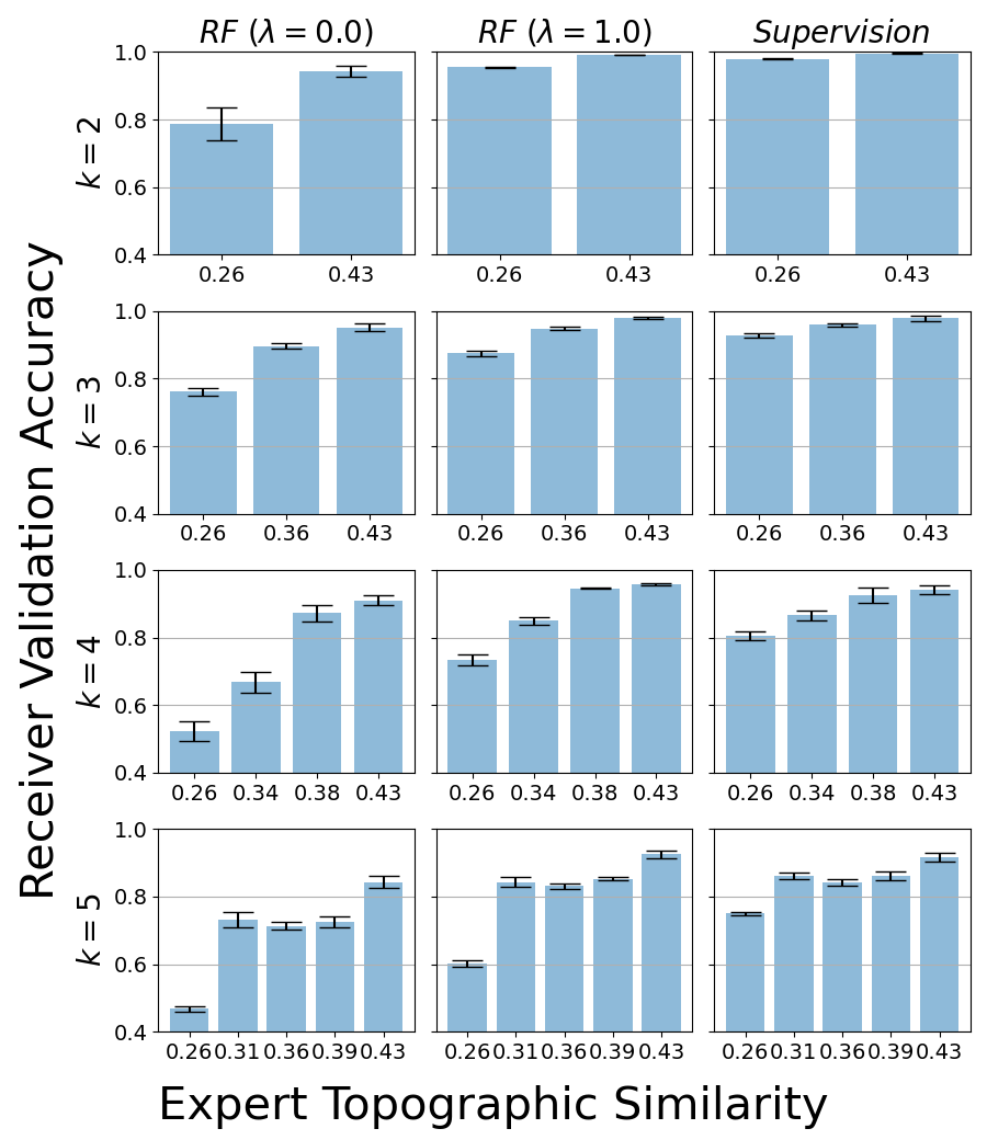
Using all Expert topsim distributions generated so far (those where topsim ranks are evenly spaced, and those exhibiting varying skews), we investigate the effect of topsim distribution spread, quantified by standard deviation, on the learned weights. In fig. 4, we note a significant negative effect of Expert topsim standard deviation on the degree of compositional selection. That is, the more disperse the Expert topsims, the more the Imitator can differentiate between and select compositional Experts (shown by a more negative skew in learned Expert weights). Though this correlation is highly statistically significant for both REINFORCE and supervision, the effect is x greater for REINFORCE, demonstrating that the spread between expert compositionalities plays a more important role in the degree of selection by reinforcement.
Finally, selection is less salient as the number of Experts increases, seen by the increasing entropies and skews of Expert weights (figs. 3 and D.3). Results for may be found in appendix D.
Understanding why REINFORCE selects for compositional languages
The different results between the optimization algorithms correspond to inherent differences in learning objective. Successful imitation minimizes the Kullback-Leibler divergence between the Imitator and the Expert policies ; supervision is classically known to minimize the forward KL divergence , while reinforcement minimizes the reverse KL divergence with respect to . That is, imitation by supervision is mean-fitting while imitation by reinforcement is mode-fitting– the former learns a uniform mixture of Expert languages (see section D.4 for proof), and the latter selects the best Expert language.
4 Speed-of-Imitation May Explain Compositional Selection
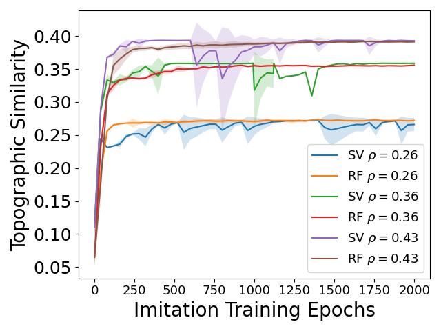
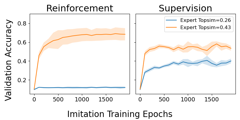
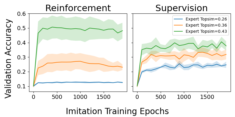
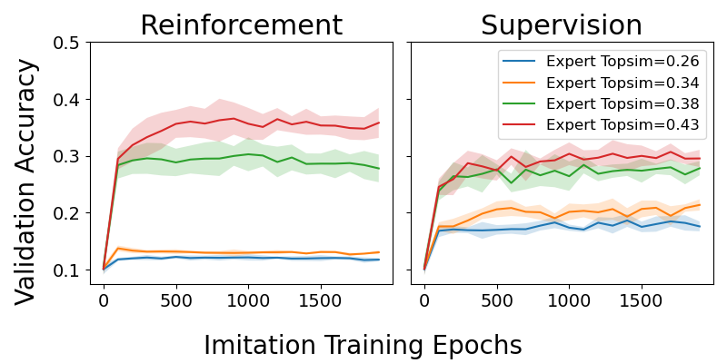
Thus far, we have seen that imitation by reinforcement selects compositional languages. This is likely because higher topsim languages are easier to imitate. We establish a positive and statistically significant relationship between topsim and ease-of-imitation, expanding the explorations in Ren et al. (2020); Li and Bowling (2019); Chaabouni et al. (2020) (see appendix C for experimental details).
We evaluate ease-of-imitation using , after (SV) and epochs (RF), where is chosen based on validation accuracy convergence. Correlations between topsims of Expert languages and Imitator performance (averaged over three random seeds) are shown in table 1. We find that for both imitation by supervision and reinforcement, topsim is (1) significantly negatively correlated to imitation sample complexity ; (2) significantly positively correlated to speed-of-imitation SOL.
| SOL | SOL | ||||
|---|---|---|---|---|---|
| SV | -0.65 | -0.80 | 0.65 | 0.75 | |
| -0.66 | -0.80 | 0.65 | 0.76 | ||
| RF | -0.66 | -0.60 | 0.45 | 0.59 | |
| -0.66 | -0.68 | 0.41* | 0.63 |
Moreover, correlations between topsim and ease-of-imitation are stronger than those between Expert validation accuracy and ease-of-imitation (table C.1). This suggests that the positive relationship between compositionality and ease-of-imitation is not due to a confound of high validation accuracy.
5 Discussion
Having (1) demonstrated a selection of compositional languages in imitation by reinforcement; (2) established a significant correlation between topsim and ease-of-imitation; we offer the following explanation for compositional selection: mode-seeking behavior in reinforcement learning exploits ease-of-learning of compositional languages, resulting in a selection of compositionality.
While both imitation and ease-of-learning of compositional languages have been instrumentalized in population training, they are engineered in a top-down way: in Chaabouni et al. (2022), agents imitate the best-accuracy agent, who is algorithmically designated as the teacher; in Ren et al. (2020), imitation is stopped early to temporally select compositional features.333We did not succeed in replicating results in Ren et al. (2020) (see appendix C). Our work, using basic RL principles, proposes an alternative mechanism that selects compositional languages while requiring minimal engineering and assumptions.
Selection by RL imitation, using the same ease-of-learning argument, applies to not only compositionality but also potentially to other traits, e.g., language entropy or message length. That is, RL imitation naturally promotes any learnability advantage among candidate languages without manual intervention, while agnostic to the signaling system. This may then be leveraged alongside communication-based learning in population-based emergent communication, where imitation would persist easy-to-learn linguistic features.
Limitations
There are several limitations to our work.
First, although we choose the attribute-value dataset due to its high degree of interpretability and control, we acknowledge that its simplicity limits the impact of our findings. Though imitation by reinforcement is a data-agnostic mechanism, we have yet to explore how it behaves in more complex settings, such as using naturalistic image inputs or embodied communication. We defer to Chaabouni et al. (2022); Galke et al. (2022) for further discussion on scaling up communication settings.
A second limitation of our results is that we do not explore how imitation-based learning scales to Experts. In particular, our hyperparameter regime handles up to around Experts– very preliminary analyses on Experts suggest a need to also scale up hyperparameters such as agent size and communication channel capacity. When training agents to imitate, one must therefore consider feasibility of the learning problem– for example, as a function of the imitation network topology, communication channel size, agent size, etc– in order for training to converge.
Finally, although our work is inspired by imitation learning in humans, the extent to which simulations explain human linguistic phenomena is not clear. We intend for our work to only serve as a testbed to understand communication from a theoretical perspective.
Ethics Statement
Because our work uses synthetic data, it has little immediate ethical impact. However, our work may enable large populations of communicating agents down the line, which could have a range of civilian or military purposes.
Acknowledgements
We would like to greatly thank Marco Baroni for feedback on experiments and manuscript; Paul Michel and Rahma Chaabouni for early feedback on research direction; the three anonymous reviewers, Jeanne Bruneau-Bongard, Roberto Dessi, Victor Chomel, Lucas Weber and members of COLT UPF for comments on the manuscript. M.R. also would like to thank Olivier Pietquin, Emmanuel Dupoux and Florian Strub.
This work was funded in part by the French government under management of Agence Nationale de la Recherche as part of the “Investissements d’avenir" program, reference ANR-19-P3IA-0001 (PRAIRIE 3IA Institute), and by the ALiEN (Autonomous Linguistic Emergence in Neural Networks) European Research Council project no. 101019291. Experiments were conducted using HPC resources from TGCC-GENCI (grant 2022-AD011013547). M.R. was supported by the MSR-Inria joint lab and granted access to the HPC resources of IDRIS under the allocation 2021-AD011012278 made by GENCI.
References
- Auersperger and Pecina (2022) Michal Auersperger and Pavel Pecina. 2022. Defending compositionality in emergent languages. In Proceedings of the 2022 Conference of the North American Chapter of the Association for Computational Linguistics: Human Language Technologies: Student Research Workshop, pages 285–291, Hybrid: Seattle, Washington + Online. Association for Computational Linguistics.
- Ba et al. (2016) Jimmy Lei Ba, Jamie Ryan Kiros, and Geoffrey E. Hinton. 2016. Layer normalization.
- Bogin et al. (2018) Ben Bogin, Mor Geva, and Jonathan Berant. 2018. Emergence of communication in an interactive world with consistent speakers. CoRR.
- Chaabouni et al. (2020) Rahma Chaabouni, Eugene Kharitonov, Diane Bouchacourt, Emmanuel Dupoux, and Marco Baroni. 2020. Compositionality and generalization in emergent languages. In Proceedings of the 58th Annual Meeting of the Association for Computational Linguistics, pages 4427–4442, Online. Association for Computational Linguistics.
- Chaabouni et al. (2022) Rahma Chaabouni, Florian Strub, Florent Altché, Eugene Tarassov, Corentin Tallec, Elnaz Davoodi, Kory Wallace Mathewson, Olivier Tieleman, Angeliki Lazaridou, and Bilal Piot. 2022. Emergent communication at scale. In International Conference on Learning Representations.
- Cho et al. (2014) Kyunghyun Cho, Bart van Merriënboer, Dzmitry Bahdanau, and Yoshua Bengio. 2014. On the properties of neural machine translation: Encoder–decoder approaches. In Proceedings of SSST-8, Eighth Workshop on Syntax, Semantics and Structure in Statistical Translation, pages 103–111, Doha, Qatar. Association for Computational Linguistics.
- Galke et al. (2022) Lukas Galke, Yoav Ram, and Limor Raviv. 2022. Emergent communication for understanding human language evolution: What’s missing?
- Havrylov and Titov (2017) Serhii Havrylov and Ivan Titov. 2017. Emergence of language with multi-agent games: Learning to communicate with sequences of symbols. In Advances in Neural Information Processing Systems, volume 30. Curran Associates, Inc.
- Kharitonov and Baroni (2020) Eugene Kharitonov and Marco Baroni. 2020. Emergent language generalization and acquisition speed are not tied to compositionality. In Proceedings of the Third BlackboxNLP Workshop on Analyzing and Interpreting Neural Networks for NLP, pages 11–15, Online. Association for Computational Linguistics.
- Kharitonov et al. (2021) Eugene Kharitonov, Roberto Dessì, Rahma Chaabouni, Diane Bouchacourt, and Marco Baroni. 2021. EGG: a toolkit for research on Emergence of lanGuage in Games. https://github.com/facebookresearch/EGG.
- Kirby and Brighton (2006) Simon Kirby and Henry Brighton. 2006. Understanding linguistic evolution by visualizing the emergence of topographic mappings. Artifical Life.
- Kottur et al. (2017) Satwik Kottur, José M. F. Moura, Stefan Lee, and Dhruv Batra. 2017. Natural language does not emerge ’naturally’ in multi-agent dialog.
- Kymissis and Poulson (1990) E Kymissis and C L Poulson. 1990. The history of imitation in learning theory: the language acquisition process. Journal of the Experimental Analysis of Behavior, 54(2):113–127.
- Lazaridou and Baroni (2020) Angeliki Lazaridou and Marco Baroni. 2020. Emergent multi-agent communication in the deep learning era.
- Lazaridou et al. (2017) Angeliki Lazaridou, Alexander Peysakhovich, and Marco Baroni. 2017. Multi-agent cooperation and the emergence of (natural) language. In International Conference on Learning Representations.
- Lewis (1969) David Kellogg Lewis. 1969. Convention: A Philosophical Study. Cambridge, MA, USA: Wiley-Blackwell.
- Li and Bowling (2019) Fushan Li and Michael Bowling. 2019. Ease-of-teaching and language structure from emergent communication. In Advances in Neural Information Processing Systems, volume 32. Curran Associates, Inc.
- Raviv et al. (2021) Limor Raviv, Marianne de Heer Kloots, and Antje Meyer. 2021. What makes a language easy to learn? a preregistered study on how systematic structure and community size affect language learnability. Cognition, 210:104620.
- Ren et al. (2020) Yi Ren, Shangmin Guo, Matthieu Labeau, Shay B. Cohen, and Simon Kirby. 2020. Compositional languages emerge in a neural iterated learning model. In International Conference on Learning Representations.
- Rita et al. (2022a) Mathieu Rita, Florian Strub, Jean-Bastien Grill, Olivier Pietquin, and Emmanuel Dupoux. 2022a. On the role of population heterogeneity in emergent communication. In International Conference on Learning Representations.
- Rita et al. (2022b) Mathieu Rita, Corentin Tallec, Paul Michel, Jean-Bastien Grill, Olivier Pietquin, Emmanuel Dupoux, and Florian Strub. 2022b. Emergent communication: Generalization and overfitting in lewis games. In Advances in Neural Information Processing Systems.
- Szabo (2020) Zoltan Gendler Szabo. 2020. Compositionality. In Edward N. Zalta, editor, The Stanford Encyclopedia of Philosophy, Fall 2020 edition. Metaphysics Research Lab, Stanford University.
- Williams (1992) Ronald J. Williams. 1992. Simple statistical gradient-following algorithms for connectionist reinforcement learning. Mach. Learn., 8(3–4):229–256.
- Williams and Peng (1991) Ronald J. Williams and Jing Peng. 1991. Function optimization using connectionist reinforcement learning algorithms. Connection Science, 3(3):241–268.
Appendix A Expert Training
A.1 Reconstruction Task
In the reconstruction task, a Sender observes an object with several attributes, encoding it in a message to the Receiver, and the Receiver decodes this message to reconstruct the object. Formally,
-
1.
The Sender network receives a vector input and constructs a message of fixed length . Each symbol is taken from the vocabulary .
-
2.
The Receiver network receives and outputs , a reconstruction of .
-
3.
Agents are successful if .
Optimization
In the reconstruction task, the cross-entropy loss is computed between and , and backpropagated directly to the Receiver. The same loss is propagated to the Sender via REINFORCE. When training with REINFORCE, we also employ an entropy regularization coefficient and subtract a running mean baseline from the reward to improve training stability.
Let the Sender policy be and the Receiver be . Let refer to the one-hot vector in indexed by , which corresponds to one attribute. Then, the Receiver’s supervised loss is as follows:
| (3) |
Let the Sender reward at time be , and let be a running mean of . Then, the Sender’s REINFORCE policy loss at time is as follows:
| (4) |
Finally, loss is optimized by Adam’s default parameters (), with a learning rate of 0.005.
A.2 Experimental Details
We train 30 Expert pairs on the reconstruction task over 1000 epochs. Expert pairs converge to high validation accuracy and generalize to the in-distribution set well (statistics in table A.2).
A.3 Expert Compositionality Distributions
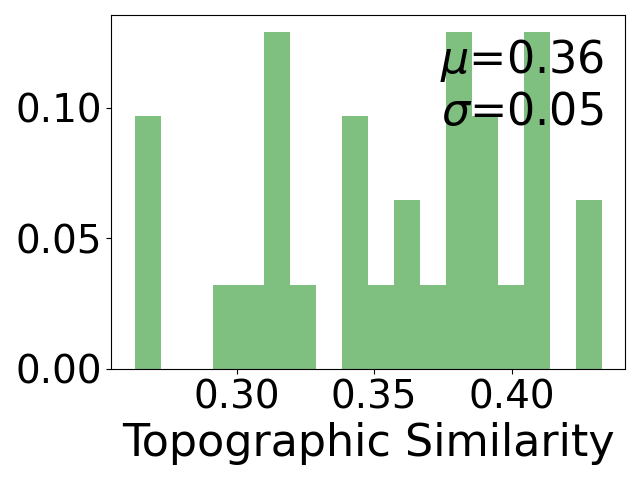
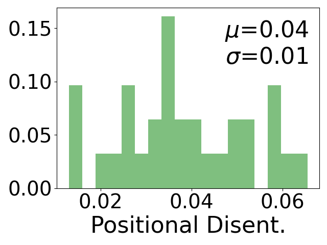
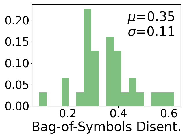
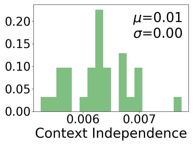
We considered using topsim, positional disentanglement (posdis) Chaabouni et al. (2020), bag-of-symbols disentanglement (bosdis) Chaabouni et al. (2020), and context independence (ci) Bogin et al. (2018) for our experiments (see fig. A.1 for distributions). However, as a fundamental reason we care about compositionality is due to its link to linguistic generalization, we focus on topsim, which we found has the highest correlation with generalization accuracy on the reconstruction task (table A.1).
Topographic similarity and generalization
Similar to Rita et al. (2022a); Auersperger and Pecina (2022) and in contrast to Chaabouni et al. (2020); Kharitonov and Baroni (2020), we find that correlations between topsim and both in-distribution and zero-shot generalization on the reconstruction task are high, and highly significant (-): Spearman’s and Pearson’s for in-distribution generalization, and , for zero-shot generalization. This correlation is stronger than that between generalization and validation accuracy, where for in-distribution generalization and for zero-shot generalization (-). Furthermore, the correlation between topsim and validation accuracy is only (-) suggesting that the relationship between generalization and compositionality is not explained by high validation accuracy.444We do not report the Pearson for Expert validation accuracy as the its distribution violates normality assumptions according to a Shapiro-Wilk non-normality test (-)). Our results support the stance in Auersperger and Pecina (2022) that compositionality, when evaluated on a suitably large dataset, indeed predicts generalization.
 |
 |
 |
 |
| topsim | bosdis | posdis | ci | |
|---|---|---|---|---|
| 0.81*** | 0.74*** | 0.29 | 0.23 | |
| 0.83*** | 0.78*** | 0.34* | 0.09 |
| Metric | Value |
|---|---|
| Validation acc. (per-object) | |
| Validation acc. (per-attribute) | |
| Generalization acc. (obj.) | |
| Generalization acc. (att.) | |
| Zero-shot gen. acc. (obj.) | |
| Zero-shot gen. acc. (att.) |
Appendix B Implementation Details
B.1 Model Architecture
Both agents are single-layer recurrent neural networks that are deterministic after training.
The Sender is a single-layer GRU Cho et al. (2014) containing a fully-connected (FC) layer that maps the input to its first hidden state (dim=). A symbol is then generated by applying an FC layer to its hidden state, and sampling from a categorical distribution parameterized by the output. We include LayerNorm Ba et al. (2016) after the hidden state to improve training stability. Then, the next input to the GRU is the previous output, which is sampled during training and argmax-ed during evaluation. This input is fed through an embedding module (dim=), which then gets fed into the GRU. The first input is the [SOS] token, and the Sender is unrolled for timesteps to output symbols comprising a message. Only in imitation training, when unrolling the Imitator Sender, we take the Expert Sender’s previous output to be the Imitator’s next input so that the Imitator learns an autoregressive model of the Expert language.
The Receiver has a similar architecture to the Sender. It consists of an FC symbol-embedding layer, a GRU with LayerNorm (hidden dim=), and an FC output head. The first hidden state is initialized to all zeros, then the FC-embedded symbols of the Sender message are sequentially fed into the GRU for timesteps. We pass the GRU’s final output through a final FC layer and compute the Receiver’s distribution over objects on the result, which we interpret as a concatenation of probability vectors each of length .
B.2 Hyperparameter settings
Hyperparameters tested may be found in table B.1. These hold for all experiments unless explicitly stated otherwise.
Dataset splits
Of the datapoints in the entire dataset, the in-distribution set has size , and we randomly sample 1% to be the training set, (), and delegate the rest to the generalization set (). Finally, the zero-shot generalization set consists of inputs where one attribute assumes the held-out value, and other attributes take on seen values ().
| Hyperparameter | Values |
| Vocab size () | 10 |
| Message length () | 10 |
| # Attributes () | 6 |
| # Values () | 10 |
| Learning rate | 0.005 |
| Batch size | 1024 |
| Entropy coeff. () | 0, 0.01, 0.1, 0.5, 1 |
| GRU hidden size | 128 |
| GRU embedding size | 128 |
| Expert pretraining epochs | 1000 |
| Single imitation training epochs (RF) | 2000 |
| Single imitation training epochs (SV) | 500 |
| # Experts in imitation mixture () | 2–5 |
| Sender imitation training epochs | 2000 |
| Rcvr imitation training epochs | 7000 |
B.3 Implementation Details
Experiments were implemented using PyTorch and the EGG toolkit Kharitonov et al. (2021). They were carried out on a high-performance cluster equipped with NVIDIA GPUs. The number of GPU-hours to run all experiments is estimated to be between 50 and 100.
Appendix C Supplementary Material: Ease-of-Imitation
In the compositionality vs. ease-of-imitation experiments, we train newly initialized Imitator pairs on each Expert pair over 500 epochs for supervision and 2000 epochs for reinforcement, aggregating over 3 random seeds. The number of training epochs is chosen by visual inspection of validation accuracy convergence. We note that, when imitating by both reinforcement and supervision, there is no initial increase in topsim followed by a convergence to Expert topsim (fig. C.1), contrary to what is observed in Ren et al. (2020).
For imitation by reinforcement, we use an entropy coefficient of for both Sender and Receiver. Comparing SOL and for both Sender and Receiver to other compositionality metrics (table C.1), we see that topsim is generally most correlated with sample complexity and speed-of-learning. For the opposite reason, we did not move ahead with, e.g., experiments on positional disentanglement.
 |
 |
 |
 |
| SOL | SOL | ||||||||
|---|---|---|---|---|---|---|---|---|---|
| SV | topsim | -0.65*** | -0.66*** | -0.80*** | -0.80*** | 0.65 *** | 0.65*** | 0.75*** | 0.76*** |
| bosdis | -0.64*** | -0.67*** | -0.54*** | -0.60*** | 0.63*** | 0.71*** | 0.81*** | 0.83*** | |
| CI | -0.24 | -0.16 | -0.20 | -0.01 | 0.40** | 0.34* | 0.30* | 0.09 | |
| posdis | -0.15 | -0.18 | -0.26 | -0.26 | 0.22 | 0.23 | 0.17 | 0.16 | |
| acc | -0.53*** | – | -0.72*** | – | 0.56 *** | – | 0.53*** | – | |
| RF | topsim | -0.66*** | -0.66*** | -0.60*** | -0.68*** | 0.45*** | 0.41** | 0.59*** | 0.63*** |
| bosdis | -0.73*** | -0.72*** | -0.61*** | -0.67*** | 0.71*** | 0.75*** | 0.41** | 0.40** | |
| CI | -0.24 | -0.16 | -0.41** | -0.39** | 0.11 | -0.06 | 0.32* | 0.29 | |
| posdis | -0.03 | -0.11 | -0.43** | -0.38** | -0.1 | -0.15 | 0.25 | 0.26 | |
| acc | -0.51*** | – | -0.52*** | – | 0.28 | – | 0.23 | – | |
Appendix D Supplementary: Imitators Select Compositional Languages to Learn
 |
 |
| (a) | (b) |
D.1 Optimization
In the imitation task, we test both direct supervision and REINFORCE. Importantly, when doing a forward pass for the Sender during training, we feed it the Expert symbol from the previous timestep as input so that the Sender learns an autoregressive model of language. Hence, define the Imitator policy as in section D.4.
In the direct supervision setting, for the Sender producing a distribution over messages given and a given Expert producing message , where is the symbol of , the overall loss for a uniform mixture of Expert Senders is the following cross-entropy loss:
| (5) |
In the REINFORCE setting, we use accuracy per-symbol as a reward for the Sender, with entropy regularization and mean baseline.555We also tried REINFORCE using negative cross-entropy loss as a reward, but found training to be unstable. For Expert , this corresponds to a reward of
| (6) |
and a policy loss of
| (7) |
per Expert, which is averaged over Experts to produce the mixture-policy loss. This is optimized by Adam with a learning rate of .
D.2 Sampling Sender Expert Distributions
To test the effect of the shape (skew, standard deviation) of the Expert topsims on imitation, we define a set of 10 distributions for each setting of Experts, noting that when , the skew is mechanically equal to 0.
For interpretability, we hold the endpoints of the distributions equal at the minimum and maximum possible topsims (0.26, 0.43) for all distributions and values of . Then, we sample the median of the 10 distributions evenly from 0.26 to 0.43. Then, we fill the other points to create a uniform distribution with mean . If the median is less than the average topsim, then the left endpoint of this uniform distribution is the minimum topsim. Otherwise, it is the maximum topsim.
D.3 Effect of population size on learned Expert Sender weights
We find that the selection effect decreases as the number of Experts increases, i.e. the Expert weight distribution looks increasingly uniform (fig. D.2). We offer two possible explanations: (1) the harder learnability of this problem given our hyperparameter regime– this is suggested by the lower maximum validation accuracy achieved on any one Expert in RF– or (2) the (mechanically) smaller variance between values, holding endpoints equal, as we increase the number of agents. Notably, the purpose of this work is not to scale up to imitation in large populations of agents; we delegate the problem of operationalizing RL imitation at scale to future work.
D.4 Learning a uniform mixture of policies
Claim
A Sender that imitates a uniform mixture of Expert Senders will output a uniform mixture of the Expert languages.
Proof
Let be Expert Senders and let be the Imitator Sender. For each position in a message, agents produce a probability distribution over all possible symbols in . Recall that the Expert Senders are deterministic at evaluation time. Given an input , we write as the value of the position in the message produced by Expert .
For the Imitator Sender, we write
as the probability distribution over possible symbols in position of a message produced by the Imitator agent, given the previous output symbol of Expert . The index of , or , gives the Imitator agent’s probability of symbol at position in the message.
The ideal Imitator minimizes the cross-entropy objective between its messages and that of a uniform mixture of Expert Senders. Formally,
whose unique solution is , , i.e. a uniform distribution over Expert languages.
Appendix E Receiver imitation
E.1 Setup
The Receiver imitation task is as follows: given a set of Expert Receivers and their corresponding Senders, we train an identical, newly initialized Receiver on the Experts’ inputs and outputs . That is, for each round of training, all Experts as well as the Imitator Receiver receive input , or the output of Expert Sender given , and output and , respectively. Imitators are then tasked to minimize the difference between their output and a uniform mixture of the Expert outputs.
The architecture for the Receiver agent may be found in B.1.
Optimization
Similar to in Sender imitation, we test a supervised learning and a reinforcement imitation learning setting. For supervised learning, the Receiver imitation loss is equal to the cross-entropy loss between its output and the Expert Receiver’s output given the same corresponding Expert Sender’s message . Then, the loss over the entire mixture is the average cross-entropy loss per Receiver, aggregated across Expert Receivers.
For REINFORCE, the Receiver reward is similar to the Sender reward– analogous to the per-symbol accuracy, it is the per-attribute accuracy. We compute the corresponding policy loss (using a mean baseline per Expert and defined in table B.1), and average over all Experts to get the overall policy loss for the Receiver.
E.2 Imitation and Selection of Compositionality
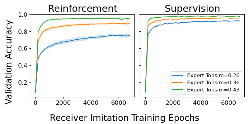
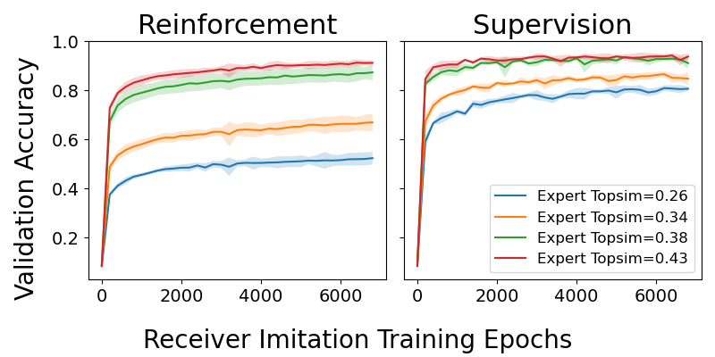
With the large communication channel size typical of emergent communication games, we can expect little Expert message collision. Then, in this setting, Receiver imitation consists of learning a many-to-one mapping of messages to outputs, obviating a real need for selection if the goal is to maximize eventual communication accuracy. Indeed, we find that Imitator Receivers learn to be multilingual, achieving high validation accuracy on all Experts, and especially in the supervised setting.
We do note, however, greater differentiation in validation accuracy, as well as speed-of-learning, between Experts of varying compositionality when using reinforcement compared to supervision, and again influenced by the entropy coefficient (figs. E.1, E.2 and E.3).
 |
 |
 |
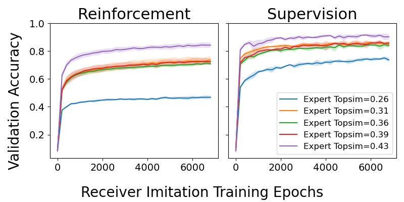 |
How one operationalizes Receiver imitation then depends on one’s goal: for example, if the goal is to maximize communication accuracy in a population of communicating agents, then we want to have “tolerant" Receivers, and imitation by supervision allows the Receiver to achieve the highest validation accuracy on all languages. However, if we want to bottleneck the compositionality of the language in the population, we want to have more “selective" Receivers, and imitation by reinforcement may be more appropriate.
E.3 Speed-of-Imitation May Explain Compositional Selection
Results for the Sender also hold for the Receiver; see section 4 for the analogous comments.