GraFITi: Graphs for Forecasting Irregularly Sampled Time Series

Abstract

Forecasting irregularly sampled time series with missing values is a crucial task for numerous real-world applications such as healthcare, astronomy, and climate sciences. State-of-the-art approaches to this problem rely on Ordinary Differential Equations (ODEs) which are known to be slow and often require additional features to handle missing values. To address this issue, we propose a novel model using Graphs for Forecasting Irregularly Sampled Time Series with missing values which we call GraFITi. GraFITi first converts the time series to a Sparsity Structure Graph which is a sparse bipartite graph, and then reformulates the forecasting problem as the edge weight prediction task in the graph. It uses the power of Graph Neural Networks to learn the graph and predict the target edge weights. GraFITi has been tested on $3$ real-world and $1$ synthetic irregularly sampled time series dataset with missing values and compared with various state-of-the-art models. The experimental results demonstrate that GraFITi improves the forecasting accuracy by up to $17\%$ and reduces the run time up to $5$ times compared to the state-of-the-art forecasting models.

1 Introduction

Time series forecasting predicts future values based on past observations. While extensively studied, most research focuses on regularly sampled and fully observed multivariate time series (MTS) (Lim and Zohren 2021; Zeng et al. 2022; De Gooijer and Hyndman 2006). Limited attention is given to irregularly sampled time series with missing values (IMTS) which is commonly seen in many real-world applications. IMTS has independently observed channels at irregular intervals, resulting in sparse data alignment. The focus of this work is on forecasting IMTS. Additionally, there is another type called irregular multivariate time series which is fully observed but with irregular time intervals (Figure 1 illustrates the differences) which is not the interest of this paper.

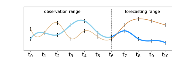
(a) Forecasting regular multivariate time series (MTS)

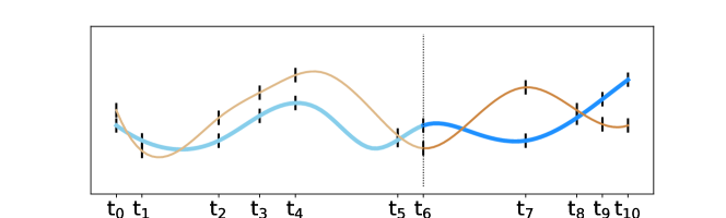
(b) Forecasting irregular multivariate time series

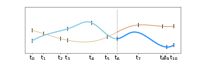
(c) Forecasting irregularly sampled multivariate time series with missing values (IMTS)

Figure 1: (a) multivariate time series forecasting, (b) irregular multivariate time series forecasting, (c) forecasting irregularly sampled multivariate time series with missing values. In all cases the observation range is from time $t_{0}$ to $t_{6}$ and the forecasting range is from time $t_{7}$ to $t_{10}$.

Ordinary Differential Equations (ODE) model continuous time series predicting system evolution over time based on the rate of change of state variables as shown in Eq. 1.

$$\frac{\mathrm{d}}{\mathrm{d}t}x(t)=f(t,x(t))$$ (1)

ODE-based models (Schirmer et al. 2022; De Brouwer et al. 2019; Biloš et al. 2021; Scholz et al. 2023) are able to forecast at arbitrary time points. However, ODE models can be slow because of their auto-regressive nature and computationally expensive numerical integration process. Also, some ODE models cannot directly handle missing values in the observation space, hence, they often rely on missing value indicators (De Brouwer et al. 2019; Biloš et al. 2021) which are given as additional channels in the data.

In this work, we propose a novel model called GraFITi: graphs for forecasting IMTS. GraFITi converts IMTS data into a Sparsity Structure Graph and formulates forecasting as edge weight prediction in the graph. This approach represents channels and timepoints as disjoint nodes connected by edges in a bipartite graph. GraFITi uses multiple graph neural network (GNN) layers with attention and feed-forward mechanisms to learn node and edge interactions. Our Sparsity Structure Graph, by design, provides a more dynamic and adaptive approach to process IMTS data, and improves the performance of the forecasting task.

We evaluated GraFITi for forecasting IMTS using $3$ real-world and $1$ synthetic dataset. Comparing it with state-of-the-art methods for IMTS and selected baselines for MTS, GraFITi provides superior forecasts.

Our contributions are summarized as follows:

• We introduce a novel representation of irregularly sampled multivariate time series with missing values (IMTS) as sparse bipartite graphs, the Sparsity Structure Graph, that efficiently can handle missing values in the observation space of the time series (Section 4).

• We propose a novel model based on this representation, GraFITi, that can leverage any graph neural network to perform time series forecasting for IMTS (section 5).

• We provide extensive experimental evaluation on $3$ real world and $1$ synthetic dataset that shows that GraFITi improves the forecasting accuracy of the best existing models by up to $17\%$ and the run time improvement up to $5$ times (section 6).

We provide the implementation at https://anonymous.4open.science/r/GraFITi-8F7B.

2 Related Work

This work focus on the forecasting of irregularly sampled multivariate time series data with missing values using graphs. In this section, we discuss the research done in: forecasting models for IMTS, Graphs for forecasting MTS, and models for edge weight prediction in graphs.

Forecasting of IMTS

Research on IMTS has mainly focused on classification (Li and Marlin 2015; Lipton, Kale, and Wetzel 2016; Rubanova, Chen, and Duvenaud 2019; Shukla and Marlin 2021; Horn et al. 2020; Tashiro et al. 2021) and interpolation (Che et al. 2018; Rubanova, Chen, and Duvenaud 2019; Shukla and Marlin 2021; Tashiro et al. 2021; Shukla and Marlin 2022; Yalavarthi, Burchert, and Schmidt-Thieme 2022), with limited attention to forecasting tasks. Existing models for these tasks mostly rely on Neural ODEs (Che et al. 2018). In Latent-ODE (Rubanova, Chen, and Duvenaud 2019), an ODE was combined with a Recurrent Neural Network (RNN) for updating the state at the point of new observation. The GRU-ODE-Bayes model (De Brouwer et al. 2019) improved upon this approach by incorporating GRUs, ODEs, and Bayesian inference for parameter estimation. The Continuous Recurrent Unit (CRU) (Schirmer et al. 2022) based model uses a state-space model with stochastic differential equations and kalman filtering. The recent LinODENet model (Scholz et al. 2023) enhanced CRU by using linear ODEs and ensure self-consistency in the forecasts. Another branch of study involves Neural Flows (Biloš et al. 2021), which use neural networks to model ODE solution curves, rendering the ODE integrator unnecessary. Among various flow architectures, GRU flows have shown good performance.

Using graphs for MTS

In addition to CNNs, RNNs, and Transformers, graph-based methods have been studied for IMTS forecasting. Early GNN-based approaches, such as (Wu et al. 2020), required a pre-defined adjacency matrix to establish relationships between the time series channels. More recent models like the Spectral Temporal Graph Neural Network (Cao et al. 2020) (STGNN) and the Time-Aware Zigzag Network (Chen, Segovia, and Gel 2021) improved on this by using GNNs to capture dependencies between variables in the time series. On the other hand, Satorras, Rangapuram, and Januschowski (2022) proposed a bipartite setup with induced nodes to reduce graph complexity, built solely from the channels. Existing graph-based time series forecasting models focus on learning correlations or similarities between channels, without fully exploiting the graph structure. Recently, GNNs were used for imputation and reconstruction of MTS with missing values, treating MTS as sequences of graphs where nodes represent sensors and edges denote correlation (Cini, Marisca, and Alippi 2022; Marisca, Cini, and Alippi 2022). Similar to previous studies, they learn similarity or correlation among channels.

Graph Neural Networks for edge weight prediction

Graph Neural Networks (GNNs) are designed to process graph-based data. While most GNN literature such as Graph Convolutional Networks, Graph Attention Networks focuses on node classification (Kipf and Welling 2017; Velickovic et al. 2017), a few studies have addressed edge weight prediction. Existing methods  (De Sá and Prudêncio 2011; Fu et al. 2018) in this domain rely on latent features and graph heuristics, such as node similarity (Zhao et al. 2015), proximity measures (Murata and Moriyasu 2007), and local rankings (Yang and Wang 2020). Recently, deep learning-based approaches (Hou and Holder 2017; Zulaika et al. 2022; You et al. 2020) were proposed. Another branch of research deals with edge weight prediction in weighted signed graphs (Kumar et al. 2016) tailored to social networks. However, all proposed methods typically operate in a transductive setup with a single graph split into training and testing data, which may not be suitable for cases involving multiple graphs like ours, where training and evaluation need to be done on separate graph partitions.

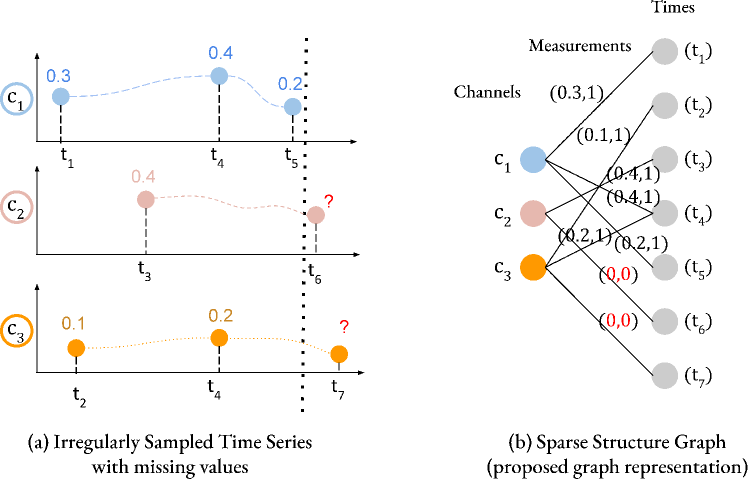
Figure 2: Representation of IMTS as Sparsity Structure Graph. (b) is the Sparsity Structure Graph representation of (a) where times and channels are the nodes and observation measurements are the edges with observations values. Target edges are provided with $\color[rgb]{1,0,0}(0,0)$.

3 The Time Series Forecasting Problem

An irregularly sampled multivariate times series with missing values, is a finite sequence of pairs $S=(t_{n},x_{n})_{n=1:N}$ where $t_{n}\in{\mathds{R}}$ is the $n$-th observation timepoint and $x_{n}\in({\mathds{R}}\cup\{\texttt{NaN}\})^{C}$ is the $n$-th observation event. Components with $x_{n,c}\neq\texttt{NaN}$ represent observed values by channel $c$ at event time $t_{n}$, and $x_{n,c}=\texttt{NaN}$ represents a missing value. $C$ is the total number of channels.

A time series query is a pair $(Q,S)$ of a time series $S$ and a sequence $Q=(q_{k},c_{k})_{k=1:K}$ such that the value of channel $c_{k}\in\{1,\ldots,C\}$ is to be predicted at time $q_{k}\in{\mathds{R}}$. We call a query a forecasting query, if all its query timepoints are after the last timepoint of the time series $S$, an imputation query if all of them are before the last timepoint of $S$ and a mixed query otherwise. In this paper, we are interested in forecasting only.

A vector $y\in{\mathds{R}}^{K}$ we call an answer to the forecasting query: $y_{k}$ is understood as the predicated value of time series $S$ at time $q_{k}$ in channel $c_{k}$. The difference between two answers $y,y^{\prime}$ to the same query can be measured by any loss function, for example by a simple squared error

$$\ell(y,y^{\prime})\coloneqq\frac{1}{K}\sum_{k=1}^{K}(y_{k}-y_{k}^{\prime})^{2}$$

The time series forecasting problem is as follows: given a dataset of pairs $D\coloneqq(Q_{i},S_{i},y_{i})_{i=1:M}$ of forecasting queries and ground truth answers from an unknown distribution $p^{\text{data}}$ and a loss function $\ell$ on forecasting answers, find a forecasting model $\hat{y}$ that maps queries $(Q,S)$ to answers $\hat{y}(Q,S)$ such that the expected loss between ground truth answers and forecasted answers is minimal:

$$\mathcal{L}(\hat{y};p^{\text{data}})\coloneqq\mathbb{E}_{(Q,S,y)\sim p^{\text{data}}}\big{[}\ell(y,\hat{y}(Q,S))\big{]}$$

4 Sparsity Structure Graph Representation

We describe the proposed Sparsity Structure Graph representation and convert the forecasting problem as edge weight prediction problem. Using the proposed representation:

• We explicitly obtain the relationship between the channels and times via observation values allowing the inductive bias of the data to pass into the model.

• We elegantly handle the missing values in IMTS in the observation space by connecting edges only for the observed values.

Missing values represented by NaN-values are unsuited for standard arithmetical operations. Therefore, they are often encoded by dedicated binary variables called missing value indicators or masks: $x_{n}\in({\mathds{R}}\times\{0,1\})^{C}$. Here, $(x_{n,c,1},1)$ encodes an observed value and $(0,0)$ encodes a missing value. Usually, both components are seen as different scalar variables: the real value $x_{n,c,1}$ and its binary missing value indicator / mask $x_{n,c,2}$, the relation between both is dropped and observations simply modeled as $x_{n}\in{\mathds{R}}^{2C}$.

We propose a novel representation of a time series $S$ using a bipartite graph $G=(V,E)$. The graph has nodes for channels and timepoints, denoted as $V_{C}$ and $V_{T}$ respectively ($V=V_{C}\mathbin{\dot{\cup}}V_{T}$). Edges $E\subseteq V_{C}\times V_{T}$ in the graph connect each channel node to its corresponding timepoint node with an observation. Edge features $F^{\text{edge}}$ are the observation values and node features $F^{\text{node}}$ are the channel IDs and timepoints. Nodes $V_{C}\coloneqq\{1,\ldots,C\}$ represent channels and nodes $V_{T}\coloneqq\{C+1,\ldots,C+N\}$ represent unique timepoints:

$$\begin{aligned} V&\coloneqq\{1,\ldots,C+N\}=V_{C}\mathbin{\dot{\cup}}V_{T}\\ E&\coloneqq\bigl{\{}\{i,j\}\mid x_{i-C,j}\neq\texttt{NaN},i\in V_{T},j\in V_{C}\bigr{\}}\\ F^{\text{node}}_{v}&\coloneqq\begin{cases}v\hfill:&v\in V_{C}\\ t_{j}\hfill:&v\in V_{T},\;j=v-C\end{cases}\\ F^{\text{edge}}_{e}&\coloneqq x_{i-C,j}\mbox{\quad for\quad}e=\{i,j\}\in E\mbox{\quad with\quad}i\in V_{T},j\in V_{C}\end{aligned}$$ (2)

For an IMTS, missing values make the bipartite graph sparse, meaning $|E|\ll C\cdot N$. However, for a fully observed time series, where there are no missing values, i.e. $|E|=C\cdot N$, the graph is a complete bipartite graph.

We extend this representation to time series queries $(S,Q)$ by adding additional edges between queried channels and timepoints, and distinguish observed and queried edges by an additional binary edge feature called target indicator. Note that the target indicator used to differentiate the observed edge and target edge is different from the missing value indicator which is used to represent the missing observations in the observation space. Given a query $Q=(q_{k},c_{k})_{k=1:K}$, let $(t^{\prime}_{1},\ldots,t^{\prime}_{K^{\prime}})$ be an enumeration of the unique queried timepoints $q_{k}$. We introduce additional nodes $V_{Q}\coloneqq\{C+N+1,\ldots,C+N+K^{\prime}\}$ so that the augmented graph, together with the node and edge features is given as

$$\begin{aligned} V&\coloneqq V_{C}\mathbin{\dot{\cup}}V_{T}\mathbin{\dot{\cup}}V_{Q}=\{1,\ldots,C+N+K^{\prime}\}\\ E&\coloneqq\bigl{\{}\{i,j\}\mid x_{i-C,j}\neq\texttt{NaN},i\in V_{T},j\in V_{C}\bigr{\}}\\ &\quad\cup\bigl{\{}\{i,j\}\mid i\in V_{Q},j\in V_{C},(t^{\prime}_{i-N-C},j)\in Q\bigr{\}}\\ F^{\text{node}}_{v}&\coloneqq\begin{cases}v\hfill:&v\in V_{C}\\ t_{j}\hfill:&v\in V_{T},j=v-C\\ t^{\prime}_{j}\hfill:&v\in V_{Q},j=v-C-N\end{cases}\\ F^{\text{edge}}_{e}&\coloneqq\begin{cases}(x_{i,j,1},1)\hfill:&e=\{i,j\}\in E,\quad i\in V_{T},j\in V_{C}\\ (0,0)\hfill:&e=\{i,j\}\in E,\quad i\in V_{Q},j\in V_{C}\\ \end{cases}\end{aligned}\;$$ (3)

where $(t^{\prime}_{i-N-C},j)\in Q$ is supposed to mean that $(t^{\prime}_{i-N-C},j)$ appears in the sequence $Q$. To denote this graph representation, we write briefly

$$\text{ts2graph}(X,Q)\coloneqq(V,E,F^{\text{node}},F^{\text{edge}})$$ (4)

The conversion of an IMTS to a Sparsity Structure Graph is shown in Figure 2.

To make the graph representation $(V,E,F^{\text{node}},F^{\text{edge}})$ of a time series query processable by a graph neural network, node and edge features have to be properly embedded, otherwise, both, the nominal channel ID and the timepoint are hard to compute on. We propose an Initial Embedding layer that encodes channel IDs via a onehot encoding and time points via a learned sinusoidal encoding (Shukla and Marlin 2021):

$$h_{v}^{\text{node},0} \coloneqq\begin{cases}\mathbf{FF}(\text{onehot}(F^{\text{node}}_{v}))&:v\in V_{C}\\ \sin(\mathbf{FF}(F^{\text{node}}_{v}))&:v\in V_{T}\mathbin{\dot{\cup}}V_{Q}\end{cases}$$ (5)

$$h_{e}^{\text{edge},0} \coloneqq\mathbf{FF}(F^{\text{edge}}_{e})\mbox{\quad for\quad}e\in E$$ (6)

where onehot denotes the binary indicator vector and $\mathbf{FF}$ denotes a separate fully connected layer in each case.

The final graph neural network layer $(h^{\text{node},L},h^{\text{edge},L})$ has embedding dimension $1$. The scalar values of the query edges are taken as the predicted answers to the encoded forecasting query:

$$\hat{y} \coloneqq\text{graph2ts}(h^{\text{node},L},h^{\text{edge},L},V,E)=(h^{\text{edge},L}_{e_{k}})_{k=1:K}$$

$$\phantom{{}\coloneqq{}}\text{where }e_{k}=\{C+N+k^{\prime},c_{k}\}\mbox{\quad with\quad}t^{\prime}_{k^{\prime}}=q_{k}$$ (7)

5 Forecasting with GraFITi

GraFITi first encodes the time series query to graph using Eq. 4 and compute initial embeddings for the nodes ($h^{\text{node},{0}}$) and edges ($h^{\text{edge},{0}}$) using Eqs. 5 and 6 respectively. Now, we can leverage the power of graph neural networks for further processing the encoded graph. Node and edge features are updated layer wise, from layer $l$ to $l+1$ using a graph neural network:

$$(h^{\text{node},{l+1}},h^{\text{edge},{l+1}})\coloneqq\text{gnn}^{(l)}(h^{\text{node},{l}},h^{\text{edge},{l}},V,E)$$ (8)

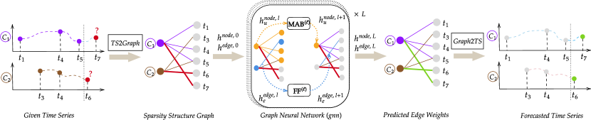
Figure 3: Overall architecture of GraFITi.

There have been a variety of gnn architectures such as Graph Convolutional Networks (Kipf and Welling 2017), Graph Attention Networks (Velickovic et al. 2017), proposed in the literature. In this work, we propose a model adapting the Graph Attention Network (Velickovic et al. 2017) to our graph setting and incorporate essential components for handling sparsity structure graphs. While a Graph Attention Network computes attention weights by adding queries and keys, we found no advantage in using this approach (see supplementary material). Thus, we utilize standard attention mechanism, in our attention block, as it has been widely used in the literature (Zhou et al. 2021). Additionally, we also use edge embeddings in our setup to update node embeddings in a principled manner.

Graph Neural Network (gnn)

First, we define Multi-head Attention block (MAB) and Neighborhood functions that are used in our gnn.

A Multi-head attention block (MAB) (Vaswani et al. 2017) is represented as:

$$\textbf{MAB}(\mathcal{Q},\mathcal{K},\mathcal{V}) \coloneqq\alpha(\mathcal{H}+\textbf{FF}(\mathcal{H}))$$

$$\text{where}\quad\mathcal{H} \coloneqq\alpha(\mathcal{Q}+\textbf{MHA}(\mathcal{Q},\mathcal{K},\mathcal{V}))$$ (9)

where $\mathcal{Q},\mathcal{K}$ and, $\mathcal{V}$ are called queries, keys, and values respectively, MHA is multi-head attention (Vaswani et al. 2017), $\alpha$ is a non-linear activation.

The Neighborhood of a node $u$ is defined as the set of all the nodes connected to $u$ through edges in $E$:

$$\mathcal{N}(u)\coloneqq\{v\mid\{u,v\}\in{E}\}$$ (10)

GraFITi consists of $L$ gnnlayers. In each layer, node embeddings are updated using neighbor node embeddings and edge embeddings connecting them. For edge embeddings, we use the embeddings of the adjacent nodes and the current edge embedding. The overall architecture of GraFITi is shown in Figure 3.

Update node embeddings

To update embedding of a node $u\in V$, first, we create a sequence of features $H_{u}$ concatenating its neighbor node embedding $h^{\text{node},{l}}_{v}$ and edge embedding $h^{\text{edge},{l}}_{e},e=\{u,v\}$ where $v\in\mathcal{N}(u)$. We then pass $h^{\text{node},{l}}_{u}$ as queries and $H_{u}$ as keys and values to $\mathbf{MAB}$.

$$h^{\text{node},{l+1}}_{u} \coloneqq\textbf{MAB}^{(l)}\left(h^{\text{node},{l}}_{u},H_{u},H_{u}\right)$$ (11)

$$H_{u} \coloneqq\bigl{(}[h^{\text{node},{l}}_{v}\mathbin{\|}\,h^{\text{edge},{l}}_{e}]\bigr{)}_{v\in\mathcal{N}(u)},\;e=\{u,v\}$$ (12)

Updating edge embeddings:

To compute edge embedding $h^{\text{edge},{l+1}}_{e}$, $e=\{u,v\}$ we concatenate $h^{\text{node},{l}}_{u},h^{\text{node},{l}}_{v}$ and $h^{\text{edge},{l}}_{e}$, and pass it through a dense layer ($\mathbf{FF}$) followed by a residual connection and nonlinear activation.

$$h^{\text{edge},{l+1}}_{e}\coloneqq\alpha\left(h^{\text{edge},{l}}_{e}+\mathbf{FF}^{(l)}\left(h^{\text{node},{l}}_{u}\mathbin{\|}h^{\text{node},{l}}_{v}\mathbin{\|}h^{\text{edge},{l}}_{e}\right)\right)$$ (13)

where $e=\{u,v\}$. Note that, although our edges are undirected, we compute the edge embedding by concatenating the embeddings in a specific order i.e., the channel embedding, time embedding and edge embedding. We show the process of updating nodes and edges in layer $l$ using a gnnin Algorithm 1.

Algorithm 1 Graph Neural Network ($\text{gnn}^{(l)}$)

0:  $h^{\text{node},{l}},h^{\text{edge},{l}},V,E$

  for $u\in{V}$ do

     $H_{u}\leftarrow\bigl{(}[h^{\text{node},{l}}_{v}\mathbin{\|}\,h^{\text{edge},{l}}_{e}]\bigr{)}_{v\in\mathcal{N}(u)}$ //$e=\{u,v\}$

     $h^{\text{node},{l+1}}_{u}\leftarrow\textbf{MAB}^{(l)}(h^{\text{node},{l}}_{u},H_{u},H_{u})$

  for $e=\{u,v\}\in{E}$ do

     $h^{\text{edge},{l+1}}_{e}\leftarrow\alpha\left(h^{\text{edge},{l}}_{e}+\mathbf{FF}^{(l)}\left(\bigl{[}h^{\text{node},{l}}_{u}\mathbin{\|}h^{\text{node},{l}}_{v}\mathbin{\|}h^{\text{edge},{l}}_{e}\bigr{]}\right)\right)$

  return  $h^{\text{node},{l+1}},h^{\text{edge},{l+1}}$

Answering the queries:

As mentioned in Section 4, our last ${\text{gnn}}^{(L)}$ layer has embedding dimension $1$. Hence, after processing the graph features through $L$ many gnn layers, we use Eq. 4 to decode the graph and provide the predicted answers to the time series query. A forward pass of GraFITi is presented in Algorithm 2.

Algorithm 2 Forward pass of GraFITi

0:  Observed time series forecasting query $(S,Q)$

  $(V,E,F_{\text{node}},F_{\text{edge}})\leftarrow\text{ts2graph}(S,Q)$ //Eq. 4 //Initial embeddings of nodes and edges

  $h^{\text{node},{0}}\leftarrow\{h^{\text{node},{0}}_{u}\mid u\in{V}\}$ //Eq. 5

  $h^{\text{edge},{0}}\leftarrow\{h^{\text{edge},{0}}_{u,v}\mid\{u,v\}\in{E}\}$ //Eq: 6 //Graph Neural Network

  for $l\in\{1,\ldots,L\}$ do

     $h^{\text{node},{l+1}},h^{\text{edge},{l+1}}\leftarrow\text{gnn}^{(l)}(h^{\text{node},{l}},h^{\text{edge},{l}},V,E)$ //Alg. 1

  $\hat{y}\leftarrow\text{graph2ts}(h^{\text{node},{L}},h^{\text{edge},{L}},V,E)$ //Eq: 4

  return  $\hat{y}$

Computational Complexity:

The computational complexity of GraFITi primarily comes from using MAB in Eq. 11. For a single channel node $u\in\{1,...,C\}$, the maximum complexity for computing its embedding is $\mathcal{N}(u)$ since only neighborhood connections are used for the update, and $\mathcal{N}(u)\subseteq\{C+1,...,C+N+K^{\prime}\}$. Thus, computing the embeddings of all channel nodes is $\mathcal{O}(|E|)$. Similarly, the computational complexity of MAB for computing the embeddings of all nodes in $V_{T}\mathbin{\dot{\cup}}V_{Q}$ is also $\mathcal{O}(|E|)$. A feed forward layer $\mathbf{FF}:{\mathds{R}}^{Y}\to{\mathds{R}}^{Z}$ will have a computational complexity of $\mathcal{O}(YZ)$.

Delineating from GRAPE (You et al. 2020)

You et al. (2020) introduced GRAPE, a graph-based model for imputing and classifying vector datasets with missing values. This approach employs a bipartite graph, with nodes divided into separate sets for sample IDs and sample features. The edges of this graph represent the feature values associated with the samples. Notably, GRAPE learns in a transductive manner, encompassing all the data samples, including those from the test set, within in the graph. In contrast, GraFITi uses inductive approach. Here, each instance is a Sparsity Structure Graph, tailored for time series data. In this structure, nodes are divided into distinct sets for channels and timepoints, while the edges are the time series observations.

6 Experiments

Table 1: Statistics of the datasets used in the experiments. Sparsity means the percentage of missing observations in the time series

Name	#Sample	#Chann.	Max.len.	Max.Obs.	Sparsity
USHCN	1,100	5	290	320	$77.9\%$
MIMIC-III	21,000	96	96	710	$94.2\%$
MIMIC-IV	18,000	102	710	1340	$97.8\%$
Physionet’12	12,000	37	48	520	$85.7\%$

6.1 Dataset description

$4$ datasets including $3$ real world medical and $1$ synthetic climate IMTS datasets are used for evaluating the proposed model. Basic statistics of the datasets is provided in Table 1.

Physionet’12 (Silva et al. 2012) consists of ICU patient records observed for $48$ hours. MIMIC-III (Johnson et al. 2016) is also a medical dataset that consists measurements of the ICU patients observed for $48$ hours. MIMIC-IV (Johnson et al. 2021) is built upon the MIMIC-III database. USHCN (Menne, Williams Jr, and Vose 2015) is a climate dataset that consists of the measurements of daily temperatures, precipitation and snow observed over $150$ years from $1218$ meteorological stations in the USA. For MIMIC-III, MIMIC-IV and USHCN, we followed the pre-processing steps provided by Scholz et al. (2023); Biloš et al. (2021); De Brouwer et al. (2019). Hence, observations in MIMIC-III and MIMIC-IV are rounded for $30$ mins and $1$ hour respectively. Whereas for the Physionet’12, we follow the protocol of Che et al. (2018); Cao et al. (2018); Tashiro et al. (2021) and processed the dataset to have hourly observations.

Table 2: Experimental results for forecasting next three time steps. Evaluation metric MSE, Lower is better. Best results are in bold and the next best are in italics. Published results are presented in open brackets, Physionet’12 dataset was not used by the baseline models hence do not have published results. We show $\%$ improvement with $\uparrow$. ‘ME’ indicates Memory Error.

	USHCN	MIMIC-III	MIMIC-IV	Physionet’12
DLinear+	$0.347\pm 0.065$	$0.691\pm 0.016$	$0.577\pm 0.001$	$0.380\pm 0.001$
NLinear+	$0.452\pm 0.101$	$0.726\pm 0.019$	$0.620\pm 0.002$	$0.382\pm 0.001$
Informer+	$0.320\pm 0.047$	$0.512\pm 0.064$	$0.420\pm 0.007$	$0.347\pm 0.001$
FedFormer+	$2.990\pm 0.476$	$1.100\pm 0.059$	$2.135\pm 0.304$	$0.455\pm 0.004$
NeuralODE-VAE	$\quad\quad\;\,-$ ($0.960\pm 0.110$)	$\quad\quad\;\,-$ ($0.890\pm 0.010$)	$\quad\quad\;\,-$	$-$
Sequential VAE	$\quad\quad\;\,-$ ($0.830\pm 0.070$)	$\quad\quad\;\,-$ ($0.920\pm 0.090$)	$\quad\quad\;\,-$	$-$
GRU-Simple	$\quad\quad\;\,-$ ($0.750\pm 0.120$)	$\quad\quad\;\,-$ ($0.820\pm 0.050$)	$\quad\quad\;\,-$	$-$
GRU-D	$\quad\quad\;\,-$ ($0.530\pm 0.060$)	$\quad\quad\;\,-$ ($0.790\pm 0.060$)	$\quad\quad\;\,-$	$-$
T-LSTM	$\quad\quad\;\,-$ ($0.590\pm 0.110$)	$\quad\quad\;\,-$ ($0.620\pm 0.050$)	$\quad\quad\;\,-$	$-$
mTAN	$0.300\pm 0.038$	$0.540\pm 0.036$	ME	$0.315\pm 0.002$
GRU-ODE-Bayes	$0.401\pm 0.089$ (${0.430\pm 0.070})$	$0.476\pm 0.043$ (${0.480\pm 0.010}$)	$0.360\pm 0.001$ $(0.379\pm 0.005)$	$0.329\pm 0.004$
Neural Flow	$0.414\pm 0.102$	$0.477\pm 0.041$ (${0.490}\pm 0.004$)	$0.354\pm 0.001$ (${0.364}\pm 0.008$)	$0.326\pm 0.004$
CRU	$0.290\pm 0.060$	$0.592\pm 0.049$	ME	$0.379\pm 0.003$
LinODEnet	$0.300\pm 0.060$ ($0.290\pm 0.060$)	$0.446\pm 0.033$ (${0.450}\pm{0.020}$)	$0.272\pm 0.002$ ($0.274\pm 0.002$)	$0.299\pm 0.001$
GraFITi (ours)	$\mathbf{0.272\pm 0.047}$ $\quad\mathbf{\uparrow\;9.3}\%$	$\mathbf{0.396\pm 0.030}$ $\quad\mathbf{\uparrow\;11.2}\%$	$\mathbf{0.225\pm 0.001}$ $\quad\mathbf{\uparrow\;17.2\%}$	$\mathbf{0.286\pm 0.001}$ $\;\mathbf{\uparrow 4.3\%}$

6.2 Competing algorithms

Here, we provide brief details of the models that are compared with the proposed GraFITi for evaluation.

We select $4$ IMTS forecasting models for comparison, including GRU-ODE-Bayes (De Brouwer et al. 2019), Neural Flows (Biloš et al. 2021), CRU (Schirmer et al. 2022) and LinODENet (Scholz et al. 2023). Additionally, we use the well established IMTS interpolation model mTAN (Shukla and Marlin 2021). It is interesting to verify the performance of well established MTS forecasting models for IMTS setup. We do this by adding missing value indicators as the separate channels to the series and process the time series along with the missing value indicators. Hence we compare with Informer+, Fedformer+, DLinear+ and NLinear+ which are variants of Informer (Zhou et al. 2021), FedFormer (Zhou et al. 2022), DLinear and NLinear (Zeng et al. 2022) respectively. We also compare with the published results from (De Brouwer et al. 2019) for the NeuralODE-VAE (Chen et al. 2018), Sequential VAE (Krishnan, Shalit, and Sontag 2015, 2017), GRU-Simple (Che et al. 2018), GRU-D (Che et al. 2018) and T-LSTM (Baytas et al. 2017).

6.3 Experimental setup

Task protocol

We followed Scholz et al. (2023); Biloš et al. (2021); De Brouwer et al. (2019), applied 5-fold cross-validation and selected hyperparameters using a holdout validation set ($20\%$). For evaluation, we used $10\%$ unseen data. All models were trained on Mean Squared Error, which is also the evaluation metric.

Hyperparamter search

We searched the following hyperparameters for GraFITi: $L\in\{1,2,3,4\}$, #heads in MAB from $\{1,2,4\}$, and hidden nodes in dense layers from $\{16,32,64,128,256\}$. We followed the procedure of Horn et al. (2020) for selecting the hyperparameters. Specifically, we randomly sampled sets of $5$ different hyperparameters and choose the one that has the best performance on validation dataset. We used the Adam optimizer with learning rate of $0.001$, halving it when validation loss did not improve for 10 epochs. All models were trained for up to $200$ epochs, using early stopping with a patience to $30$ epochs. Hyperparameters for the baseline models are presented in the supplementary material. All the models were experimented using the PyTorch library on a GeForce RTX-3090 GPU.

6.4 Experimental results

First, we set the observation and prediction range of the IMTS following (Scholz et al. 2023; Biloš et al. 2021; De Brouwer et al. 2019). For the USHCN dataset, the model observes for the first $3$ years and forecasts the next $3$ time steps. For the medical datasets, the model observes for the first $36$ hours in the series and predicts the next $3$ time steps. The results, including the mean and standard deviation, are presented in Table 2. The best result is highlighted in bold and the next best in italics. Additionally, we also provide the published results from (Scholz et al. 2023; Biloš et al. 2021; De Brouwer et al. 2019) in brackets for comparison.

The proposed GraFITi model is shown to be superior compared to all baseline models across all the datasets. Specifically, in the MIMIC-III and MIMIC-IV datasets, GraFITi provides around $11.2\%$ and $17.2\%$ improvement in forecasting accuracy compared to the next best IMTS forecasting model LinODEnet. The results on the USHCN dataset have high variance, therefore, it is challenging to compare the models on this dataset. However, we experimented on it for completeness. Again, we achieve the best result with $9.2\%$ improvement compared to the next best model. We note that, the MTS forecasting models that are adapted for the IMTS task, perform worse than any of the IMTS forecasting models demonstrating the limitation of MTS models applied to IMTS tasks.

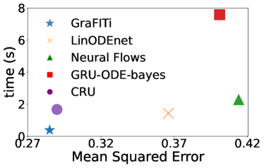
(a) USHCN

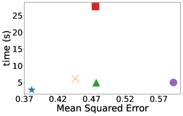
(b) MIMIC-III

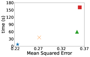
(c) MIMIC-IV

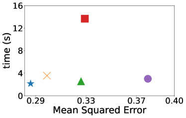
(d) Physionet’12

Figure 4: Comparison of IMTS forecasting models: GraFITi, LinODEnet, CRU, Neural Flows and GRU-ODE-Bayes in terms of efficiency: evaluation time against error metric.

Table 3: Experimental results on varying observation and forecasting ranges for the medical datasets. Evaluation measure is MSE. Lower is better. Best results are in bold and the second best are in italics. ME indicates memory error.

	Obs. $/$ Pred.	GraFITi (ours)	LinODEnet	CRU	Neural Flow	GRU-ODE-Bayes	$\quad\uparrow\%$
MIMIC-III	24/12	$\mathbf{0.438\pm 0.009}$	$\mathit{0.477\pm 0.021}$	$0.575\pm 0.020$	$0.588\pm 0.014$	$0.591\pm 0.018$	$\quad\uparrow\textbf{8.2\%}$
	24/24	$\mathbf{0.491\pm 0.014}$	$\mathit{0.531\pm 0.022}$	$0.619\pm 0.028$	$0.651\pm 0.017$	$0.653\pm 0.023$	$\quad\uparrow\textbf{7.5\%}$
	36/6	$\mathbf{0.457\pm 0.050}$	$\mathit{0.492\pm 0.019}$	$0.647\pm 0.051$	$0.573\pm 0.043$	$0.580\pm 0.049$	$\quad\uparrow\textbf{7.1\%}$
	36/12	$\mathbf{0.490\pm 0.027}$	$\mathit{0.554\pm 0.042}$	$0.680\pm 0.043$	$0.620\pm 0.035$	$0.632\pm 0.044$	$\quad\uparrow\textbf{10.8\%}$
MIMIC-IV	24/12	$\mathbf{0.285\pm 0.001}$	$\mathit{0.335\pm 0.002}$	ME	$0.465\pm 0.003$	$0.366\pm 0.154$	$\quad\uparrow\textbf{14.9\%}$
	24/24	$\mathbf{0.285\pm 0.002}$	$\mathit{0.336\pm 0.002}$	ME	$0.465\pm 0.003$	$0.439\pm 0.003$	$\quad\uparrow\textbf{15.1\%}$
	36/6	$\mathbf{0.260\pm 0.002}$	$\mathit{0.309\pm 0.002}$	ME	$0.405\pm 0.001$	$0.393\pm 0.002$	$\quad\uparrow\textbf{15.9\%}$
	36/12	$\mathbf{0.261\pm 0.005}$	$\mathit{0.309\pm 0.002}$	ME	$0.395\pm 0.001$	$0.393\pm 0.002$	$\quad\uparrow\textbf{15.5\%}$
Physionet’12	24/12	$\mathbf{0.365\pm 0.001}$	$\mathit{0.373\pm 0.001}$	$0.435\pm 0.001$	$0.431\pm 0.001$	$0.432\pm 0.003$	$\quad\uparrow\textbf{2.1\%}$
	24/24	$\mathbf{0.401\pm 0.001}$	$\mathit{0.411\pm 0.001}$	$0.467\pm 0.002$	$0.506\pm 0.002$	$0.505\pm 0.001$	$\quad\uparrow\textbf{2.4\%}$
	36/6	$\mathbf{0.319\pm 0.001}$	$\mathit{0.329\pm 0.001}$	$0.396\pm 0.003$	$0.365\pm 0.001$	$0.363\pm 0.004$	$\quad\uparrow\textbf{3.0\%}$
	36/12	$\mathbf{0.347\pm 0.001}$	$\mathit{0.357\pm 0.001}$	$0.417\pm 0.001$	$0.398\pm 0.001$	$0.401\pm 0.003$	$\quad\uparrow\textbf{2.8\%}$

Efficiency comparison

We compare the efficiency of leading IMTS forecasting models: GraFITi, LinODEnet, CRU, Neural Flow, and GRU-ODE-Bayes. We evaluate them in terms of both execution time (batch size: 64) and MSE. The results, presented in Figure 4, show that for datasets with longer time series like MIMIC-IV and USHCN, GraFITi significantly outpaces ODE and flow-based models. Specifically, GraFITi is over $5$ times faster than the fastest ODE model, LinODEnet, in both MIMIC-IV and USHCN. Even for shorter time series datasets like Physionet’12 and MIMIC-III, GraFITi remains twice as fast as LinODEnet. Moreover, on average, GraFITi surpasses GRU-ODE-Bayes in speed by an order of magnitude.

Varying observation and forecast ranges

This experiment is conducted with two different observation ranges ($24$ and $36$ hours) and two different prediction ranges for each observation range. Specifically, for the observation range of $24$ hours, the prediction ranges are $12$ and $24$ hours, and for the observation range of $36$ hours, the prediction ranges are $6$ and $12$ hours. This approach allows for a more comprehensive evaluation of the model’s performance across various scenarios of observation and prediction ranges. The results are presented in Table 3.

Again for varying observation and forecast ranges, GraFITi is the top performer, followed by LinODENet. Significant gains in forecasting accuracy are observed in the MIMIC-III and MIMIC-IV datasets. On average, GraFITi improves the accuracy of LinODEnet, the next best IMTS forecasting model, by $8.5\%$ in MIMIC-III, $15.5\%$ in MIMIC-IV, and $2.6\%$ in the Physionet’12 dataset.

Table 4: Performance of GraFITi with varying sparsity levels using MIMIC-III dataset. The ‘IMTS’ dataset refers to the actual dataset, while ‘AsTS’ is a synthetic asynchronous time series dataset created by restricting the number of observed channels at each time point to $1$. The ‘AsTS + x%’ dataset is created by modifying ‘AsTS’ dataset by retrieving x% of the missing observations. Goal is to observe $36$ hours of data and then forecast the next $3$ time steps

Model	IMTS	AsTS	AsTS+10%	AsTS+50%	AsTS+90%
GraFITi	$\mathbf{0.396}$	$0.931$	$0.845$	$\mathbf{0.547}$	$\mathbf{0.413}$
LinODENet	$0.446$	$\mathbf{0.894}$	$\mathbf{0.815}$	$0.581$	$0.452$

6.5 Limitations

The GraFITi model is a potential tool for forecasting on IMTS. It outperforms existing state-of-the-art models, even in highly sparse datasets (up to $98\%$ sparsity in MIMIC-IV). However, we note a limitation in the compatibility of the model with certain data configurations. In particular, the GraFITi faces a challenge when applied to Asynchronous Time Series datasets. In such datasets, channels are observed asynchronously at various time points, resulting in disconnected sparse graphs. This disconnection hinders the flow of information and can be problematic when channels have a strong correlation towards the forecasts as model may not be able to capture these correlations. It can be observed from Table 4 where GraFITi is compared with the next best baseline model LinODENet for varying sparsity levels using MIMIC-III dataset. The performance of GraFITi deteriorates with increase in sparsity levels and gets worst when the series become asynchronous.

Moreover, the existing model cannot handle meta data associated with the IMTS. Although, these meta data points could be introduced as additional channel nodes, this would again disconnect the graph due to lack of edges connecting the time nodes to meta data nodes. One possible solution to both the challenges is to interconnect all the channel nodes including meta data if present, and apply a distinct multi-head attention on them. Therefore, in future, we aim to enhance the capability of the proposed model to handle Asynchronous Time Series datasets and meta data in the series.

7 Conclusions

In this paper, we propose a Graph based model called GraFITi for the forecasting of irregularly sampled time series with missing values (IMTS). First we represent the time series as a Sparsity Structure Graph with channels and observation times as nodes and observation measurements as edges; and re-represent the task of time series forecasting as an edge weight prediction problem in a graph. An attention based architecture is proposed for learning the interactions between the nodes and edges in the graph. We experimented on $4$ datasets including $3$ real world and $1$ synthetic dataset for various observation and prediction ranges. The extensive experimental evaluation demonstrates that the proposed GraFITi provides superior forecasts compared to the state-of-the-art IMTS forecasting models.

Appendix A Ablation studies

A.1 Importance of target edge

In the current graph representation, target edges are connected in the graph providing rich embedding to learn the edge weight. However, we would like to see the performance of the model without query edges in the graph. For this, we compared the experimental results of GraFITi and GraFITi$\setminus$T where GraFITi$\setminus$T is the same architecture without query edges in the graph. The predictions are made after $L-1^{\text{th}}$ layer by concatenating the channel embedding and the sinusoidal embedding of the query time node and passing it through the dense layer. The results for the real IMTS datasets are reported in Table 5.

Table 5: Performance of GraFITi$\setminus$T (GraFITi without query edges in the graph), evaluation metric MSE.

Model	MIMIC-III	MIMIC-IV	Physionet’12
GraFITi	$\mathbf{0.396\pm 0.030}$	$\mathbf{0.225\pm 0.001}$	$\mathbf{0.286\pm 0.001}$
GraFITi$\setminus$T	$0.433\pm 0.019$	$0.269\pm 0.001$	$0.288\pm 0.001$

We see that the performance of the GraFITi deteriorated significantly without query edges in the graph. GraFITi exploit the sparse structure in the graph for predicting the weight of the query edge. The attention mechanism help the target edge to gather the useful information from the incident nodes.

A.2 MAB vs GAT as Graph Neural Network module gnn (Eq 8)

Table 6: Comparing performance of MAB (GraFITi-MAB) and GAT (GraFITi-GAT) as gnn module in GraFITi.

	MIMIC-III	MIMIC-IV	Physionet’12
GraFITi-MAB	$0.396\pm 0.030$	$0.225\pm 0.001$	$0.286\pm 0.001$
GraFITi-GAT	$0.388\pm 0.020$	$0.225\pm 0.001$	$0.288\pm 0.001$

In Table 6, we compare the performance of MAB and GAT as a gnn module in the proposed GraFITi. We use MIMIC-III, MIMIC-IV and Physionet’12 for the comparison. We notice that the performance of MAB and GAT are similar. Hence, we use MAB as the gnn module in the proposed GraFITi. Please note that the objective of this work is not to find the best gnn module but to show IMTS forecasting using graph neural networks.

Appendix B Hyperparameter search

We search the following hyperparameters for IMTS forecasting models as mentioned in the respective works:

GRU-ODE-Bayes:

We set the number of hidden layers to $3$ and selected solver from $\{\text{euler},\text{dopri}\}$

Neural Flows

We searched for the flow layers from $\{1,4\}$ and set the hidden layers to $2$

LinODENet

We searched for hidden size from $\{64,128\}$, latent size from $\{128,192\}$. We set the encoder with $5$-block ResNet with 2 ReLU pre-activated layers each, StackedFilter of 3 KalmanCells, with linear one in the beginning.

CRU

We searched for latent state dimension from $\{10,20,30\}$, number of basis matrices from $\{10,20\}$ and bandwidth from $\{3,10\}$.

mTAN

We searched the #attention heads from $\{1,2,4\}$, #reference time points from $\{8,16,32,64,128\}$, latent dimensions form $\{20,30,40,50\}$, generator layers from $\{25,50,100,150\}$, and reconstruction layers from $\{32,64,128,256\}$.

For the all the MTS forecasting models, we used the default hyperparameters provided in (Zeng et al. 2022).

References

- Baytas et al. (2017) Baytas, I. M.; Xiao, C.; Zhang, X.; Wang, F.; Jain, A. K.; and Zhou, J. 2017. Patient subtyping via time-aware LSTM networks. In Proceedings of the 23rd ACM SIGKDD International Conference on Knowledge Discovery and Data Mining, 65–74.
- Biloš et al. (2021) Biloš, M.; Sommer, J.; Rangapuram, S. S.; Januschowski, T.; and Günnemann, S. 2021. Neural Flows: Efficient Alternative to Neural ODEs. Advances in Neural Information Processing Systems, 34: 21325–21337.
- Cao et al. (2020) Cao, D.; Wang, Y.; Duan, J.; Zhang, C.; Zhu, X.; Huang, C.; Tong, Y.; Xu, B.; Bai, J.; Tong, J.; et al. 2020. Spectral temporal graph neural network for multivariate time-series forecasting. Advances in Neural Information Processing Systems, 33: 17766–17778.
- Cao et al. (2018) Cao, W.; Wang, D.; Li, J.; Zhou, H.; Li, L.; and Li, Y. 2018. Brits: Bidirectional recurrent imputation for time series. Advances in Neural Information Processing Systems, 31.
- Che et al. (2018) Che, Z.; Purushotham, S.; Cho, K.; Sontag, D.; and Liu, Y. 2018. Recurrent neural networks for multivariate time series with missing values. Scientific Reports, 8(1): 1–12.
- Chen et al. (2018) Chen, R. T.; Rubanova, Y.; Bettencourt, J.; and Duvenaud, D. K. 2018. Neural ordinary differential equations. Advances in Neural Information Processing Systems, 31.
- Chen, Segovia, and Gel (2021) Chen, Y.; Segovia, I.; and Gel, Y. R. 2021. Z-GCNETs: time zigzags at graph convolutional networks for time series forecasting. In International Conference on Machine Learning, 1684–1694. PMLR.
- Cini, Marisca, and Alippi (2022) Cini, A.; Marisca, I.; and Alippi, C. 2022. Filling the G_ap_s: Multivariate Time Series Imputation by Graph Neural Networks. In International Conference on Learning Representations.
- De Brouwer et al. (2019) De Brouwer, E.; Simm, J.; Arany, A.; and Moreau, Y. 2019. GRU-ODE-Bayes: Continuous modeling of sporadically-observed time series. Advances in Neural Information Processing Systems, 32.
- De Gooijer and Hyndman (2006) De Gooijer, J. G.; and Hyndman, R. J. 2006. 25 years of time series forecasting. International Journal of Forecasting, 22(3): 443–473.
- De Sá and Prudêncio (2011) De Sá, H. R.; and Prudêncio, R. B. 2011. Supervised link prediction in weighted networks. In The 2011 International Joint Conference on Neural Networks (IJCNN), 2281–2288. IEEE.
- Fu et al. (2018) Fu, C.; Zhao, M.; Fan, L.; Chen, X.; Chen, J.; Wu, Z.; Xia, Y.; and Xuan, Q. 2018. Link weight prediction using supervised learning methods and its application to yelp layered network. IEEE Transactions on Knowledge and Data Engineering, 30(8): 1507–1518.
- Horn et al. (2020) Horn, M.; Moor, M.; Bock, C.; Rieck, B.; and Borgwardt, K. 2020. Set functions for time series. In International Conference on Machine Learning, 4353–4363. PMLR.
- Hou and Holder (2017) Hou, Y.; and Holder, L. B. 2017. Deep learning approach to link weight prediction. In 2017 International Joint Conference on Neural Networks (IJCNN), 1855–1862. IEEE.
- Johnson et al. (2021) Johnson, A.; Bulgarelli, L.; Pollard, T.; Horng, S.; and Celi, L. 2021. Mark. R. MIMIC-IV (version 1.0). PhysioNet.
- Johnson et al. (2016) Johnson, A. E.; Pollard, T. J.; Shen, L.; Lehman, L.-w. H.; Feng, M.; Ghassemi, M.; Moody, B.; Szolovits, P.; Anthony Celi, L.; and Mark, R. G. 2016. MIMIC-III, a freely accessible critical care database. Scientific Data, 3(1): 1–9.
- Kipf and Welling (2017) Kipf, T. N.; and Welling, M. 2017. Semi-Supervised Classification with Graph Convolutional Networks. In International Conference on Learning Representations.
- Krishnan, Shalit, and Sontag (2017) Krishnan, R.; Shalit, U.; and Sontag, D. 2017. Structured inference networks for nonlinear state space models. In Proceedings of the AAAI Conference on Artificial Intelligence, volume 31.
- Krishnan, Shalit, and Sontag (2015) Krishnan, R. G.; Shalit, U.; and Sontag, D. 2015. Deep kalman filters. arXiv preprint arXiv:1511.05121.
- Kumar et al. (2016) Kumar, S.; Spezzano, F.; Subrahmanian, V.; and Faloutsos, C. 2016. Edge weight prediction in weighted signed networks. In 2016 IEEE 16th International Conference on Data Mining (ICDM), 221–230. IEEE.
- Li and Marlin (2015) Li, S. C.-X.; and Marlin, B. M. 2015. Classification of Sparse and Irregularly Sampled Time Series with Mixtures of Expected Gaussian Kernels and Random Features. In Proceedings of the Thirty-First Conference on Uncertainty in Artificial Intelligence, 484–493.
- Lim and Zohren (2021) Lim, B.; and Zohren, S. 2021. Time-series forecasting with deep learning: a survey. Philosophical Transactions of the Royal Society A, 379(2194): 20200209.
- Lipton, Kale, and Wetzel (2016) Lipton, Z. C.; Kale, D.; and Wetzel, R. 2016. Directly modeling missing data in sequences with rnns: Improved classification of clinical time series. In Machine Learning for Healthcare Conference, 253–270. PMLR.
- Marisca, Cini, and Alippi (2022) Marisca, I.; Cini, A.; and Alippi, C. 2022. Learning to Reconstruct Missing Data from Spatiotemporal Graphs with Sparse Observations. In The First Learning on Graphs Conference.
- Menne, Williams Jr, and Vose (2015) Menne, M. J.; Williams Jr, C.; and Vose, R. S. 2015. United States historical climatology network daily temperature, precipitation, and snow data. Carbon Dioxide Information Analysis Center, Oak Ridge National Laboratory, Oak Ridge, Tennessee.
- Murata and Moriyasu (2007) Murata, T.; and Moriyasu, S. 2007. Link prediction of social networks based on weighted proximity measures. In IEEE/WIC/ACM International Conference on Web Intelligence (WI’07), 85–88. IEEE.
- Rubanova, Chen, and Duvenaud (2019) Rubanova, Y.; Chen, R. T.; and Duvenaud, D. K. 2019. Latent ordinary differential equations for irregularly-sampled time series. Advances in Neural Information Processing Systems, 32.
- Satorras, Rangapuram, and Januschowski (2022) Satorras, V. G.; Rangapuram, S. S.; and Januschowski, T. 2022. Multivariate time series forecasting with latent graph inference. arXiv preprint arXiv:2203.03423.
- Schirmer et al. (2022) Schirmer, M.; Eltayeb, M.; Lessmann, S.; and Rudolph, M. 2022. Modeling Irregular Time Series with Continuous Recurrent Units. In Proceedings of the 39th International Conference on Machine Learning, volume 162, 19388–19405. PMLR.
- Scholz et al. (2023) Scholz, R.; Born, S.; Duong-Trung, N.; Cruz-Bournazou, M. N.; and Schmidt-Thieme, L. 2023. Latent Linear ODEs with Neural Kalman Filtering for Irregular Time Series Forecasting.
- Shukla and Marlin (2021) Shukla, S. N.; and Marlin, B. 2021. Multi-Time Attention Networks for Irregularly Sampled Time Series. In International Conference on Learning Representations.
- Shukla and Marlin (2022) Shukla, S. N.; and Marlin, B. 2022. Heteroscedastic Temporal Variational Autoencoder For Irregularly Sampled Time Series. In International Conference on Learning Representations.
- Silva et al. (2012) Silva, I.; Moody, G.; Scott, D. J.; Celi, L. A.; and Mark, R. G. 2012. Predicting in-hospital mortality of icu patients: The physionet/computing in cardiology challenge 2012. In 2012 Computing in Cardiology, 245–248. IEEE.
- Tashiro et al. (2021) Tashiro, Y.; Song, J.; Song, Y.; and Ermon, S. 2021. CSDI: Conditional score-based diffusion models for probabilistic time series imputation. Advances in Neural Information Processing Systems, 34: 24804–24816.
- Vaswani et al. (2017) Vaswani, A.; Shazeer, N.; Parmar, N.; Uszkoreit, J.; Jones, L.; Gomez, A. N.; Kaiser, Ł.; and Polosukhin, I. 2017. Attention is all you need. Advances in Neural Information Processing Systems, 30.
- Velickovic et al. (2017) Velickovic, P.; Cucurull, G.; Casanova, A.; Romero, A.; Lio, P.; and Bengio, Y. 2017. Graph attention networks. stat, 1050: 20.
- Wu et al. (2020) Wu, Z.; Pan, S.; Long, G.; Jiang, J.; Chang, X.; and Zhang, C. 2020. Connecting the dots: Multivariate time series forecasting with graph neural networks. In Proceedings of the 26th ACM SIGKDD International Conference on Knowledge Discovery & Data Mining, 753–763.
- Yalavarthi, Burchert, and Schmidt-Thieme (2022) Yalavarthi, V. K.; Burchert, J.; and Schmidt-Thieme, L. 2022. Tripletformer for Probabilistic Interpolation of Asynchronous Time Series. arXiv preprint arXiv:2210.02091.
- Yang and Wang (2020) Yang, X.; and Wang, B. 2020. Local ranking and global fusion for personalized recommendation. Applied Soft Computing, 96: 106636.
- You et al. (2020) You, J.; Ma, X.; Ding, Y.; Kochenderfer, M. J.; and Leskovec, J. 2020. Handling missing data with graph representation learning. Advances in Neural Information Processing Systems, 33: 19075–19087.
- Zeng et al. (2022) Zeng, A.; Chen, M.; Zhang, L.; and Xu, Q. 2022. Are transformers effective for time series forecasting? arXiv preprint arXiv:2205.13504.
- Zhao et al. (2015) Zhao, J.; Miao, L.; Yang, J.; Fang, H.; Zhang, Q.-M.; Nie, M.; Holme, P.; and Zhou, T. 2015. Prediction of links and weights in networks by reliable routes. Scientific reports, 5(1): 12261.
- Zhou et al. (2021) Zhou, H.; Zhang, S.; Peng, J.; Zhang, S.; Li, J.; Xiong, H.; and Zhang, W. 2021. Informer: Beyond efficient transformer for long sequence time-series forecasting. In Proceedings of the AAAI Conference on Artificial Intelligence, volume 35, 11106–11115.
- Zhou et al. (2022) Zhou, T.; Ma, Z.; Wen, Q.; Wang, X.; Sun, L.; and Jin, R. 2022. FEDformer: Frequency Enhanced Decomposed Transformer for Long-term Series Forecasting. In Proceedings of the 39th International Conference on Machine Learning, volume 162 of Proceedings of Machine Learning Research, 27268–27286. PMLR.
- Zulaika et al. (2022) Zulaika, U.; Sanchez-Corcuera, R.; Almeida, A.; and Lopez-de Ipina, D. 2022. LWP-WL: Link weight prediction based on CNNs and the Weisfeiler–Lehman algorithm. Applied Soft Computing, 120: 108657.