It’s Enough: Relaxing Diagonal Constraints in Linear Autoencoders for Recommendation

Abstract.

Linear autoencoder models learn an item-to-item weight matrix via convex optimization with L2 regularization and zero-diagonal constraints. Despite their simplicity, they have shown remarkable performance compared to sophisticated non-linear models. This paper aims to theoretically understand the properties of two terms in linear autoencoders. Through the lens of singular value decomposition (SVD) and principal component analysis (PCA), it is revealed that L2 regularization enhances the impact of high-ranked PCs. Meanwhile, zero-diagonal constraints reduce the impact of low-ranked PCs, leading to performance degradation for unpopular items. Inspired by this analysis, we propose simple-yet-effective linear autoencoder models using diagonal inequality constraints, called Relaxed Linear AutoEncoder (RLAE) and Relaxed Denoising Linear AutoEncoder (RDLAE). We prove that they generalize linear autoencoders by adjusting the degree of diagonal constraints. Experimental results demonstrate that our models are comparable or superior to state-of-the-art linear and non-linear models on six benchmark datasets; they significantly improve the accuracy of long-tail items. These results also support our theoretical insights on regularization and diagonal constraints in linear autoencoders.

1. Introduction

Over the last three decades, the field of recommender systems (Jannach et al., 2021) has been dedicated to helping users overcome information overload in various applications, e.g., Amazon, Netflix, and Bing News. Collaborative filtering (CF) (Goldberg et al., 1992; Herlocker et al., 1999) is a prevalent solution for building recommender systems due to its ability to uncover hidden collaborative signals from user-item interactions. Existing CF models can be broadly categorized into linear and non-linear approaches based on how they capture correlations among users/items. Linear models represent the user/item relationships through a linear combination. With the advent of deep learning, non-linear CF models utilize various neural networks, i.e., autoencoders (Wu et al., 2016; Liang et al., 2018; Shenbin et al., 2020; Lobel et al., 2020) (AE), recurrent neural networks (RNN) (Hidasi et al., 2016; Li et al., 2017), transformers (Kang and McAuley, 2018; Sun et al., 2019), and graph neural networks (Wang et al., 2019; Chen et al., 2020; He et al., 2020; Choi et al., 2021; Shen et al., 2021; Kong et al., 2022) (GNN). They claim that non-linear models surpass linear models in capturing intricate and scarce collaborative signals, leading to better performance in various recommendation scenarios.

However, there are exciting research debates on evaluating linear and non-linear models. Recent studies (Dacrema et al., 2019; Sun et al., 2020; Rendle et al., 2019; Dacrema et al., 2021) claim that the hyperparameters of baselines need to be tuned carefully, or the choice of evaluation metrics heavily affects a fair comparison. Surprisingly, well-tuned linear models, such as neighborhood-based models (Herlocker et al., 1999; Sarwar et al., 2001), simple graph-based models (Cooper et al., 2014; Paudel et al., 2017), and linear matrix factorization models (Zhou et al., 2008; Koren, 2008) have achieved competitive or significant gains over non-linear models. Recent linear models using item neighborhoods, e.g., EASE^R (Steck, 2019) and EDLAE (Steck, 2020), have shown state-of-the-art performance results on large-scale datasets, e.g., ML-20M, Netflix, and MSD. In this paper, we thus delve deeper into the linear models using item neighborhoods, also known as linear autoencoders (Ning and Karypis, 2011; Steck, 2019, 2020; Steck et al., 2020; Jeunen et al., 2020; Steck and Liang, 2021; Vancura et al., 2022).

Given a user-item interaction matrix $\mathbf{X}\in\{0,1\}^{m\times n}$, linear autoencoders (LAE) learn an item-to-item weight matrix $\mathbf{B}\in\mathbb{R}^{n\times n}$ so that the matrix product $\mathbf{X}\cdot\mathbf{B}$ reconstructs the original matrix $\mathbf{X}$. It takes $\mathbf{X}$ as input and output, and $\mathbf{B}$ represents a single hidden layer to serve both an encoder and a decoder. Existing studies (Ning and Karypis, 2011; Steck, 2019, 2020; Steck et al., 2020; Jeunen et al., 2020; Steck and Liang, 2021; Vancura et al., 2022) formulate a convex optimization problem with two key terms: regularization and zero-diagonal constraints. (i) Regularization is widely used to prevent the models from overfitting, i.e., $\hat{\mathbf{B}}=\mathbf{I}$. While SLIM (Ning and Karypis, 2011) utilizes both L1 and L2 regularization, EASE^R (Steck, 2019) employs only L2 regularization to derive a closed-form solution and shows better performance. However, (Steck et al., 2020) utilizes the alternating directions method of multipliers (ADMM) to optimize the objective function of SLIM, showing that L1 regularization only affects the sparsity of the solution and has little impact on recommendation results. Moreover, EDLAE (Steck, 2020) proposes linear autoencoder models with advanced regularization derived from random dropout. (ii) The zero-diagonal constraints in $\mathbf{B}$ are designed to identify precisely the correlation between items by preventing self-correlation (Ning and Karypis, 2011; Steck, 2020). Since it seems natural that the diagonal entries in $\mathbf{B}$ are unnecessary weights, existing studies (Ning and Karypis, 2011; Steck, 2019, 2020; Steck et al., 2020; Jeunen et al., 2020; Steck and Liang, 2021; Vancura et al., 2022) employ the zero-diagonal constraints to eliminate them. However, how the regularization and the zero-diagonal constraints affect recommendation is unexplored.

In this paper, we ask two underlying questions about linear autoencoder models: (i) How does each term in linear autoencoders, i.e., regularization and zero-diagonal constraints, affect item popularity? (ii) Do the zero-diagonal constraints always help improve model performance? To answer these questions, we conduct a theoretical analysis of various linear autoencoder models. We rigorously derive the relationship among four linear autoencoder models, i.e., LAE (Hoerl and Kennard, 2000), EASE^R (Steck, 2019), DLAE (Steck, 2020), and EDLAE (Steck, 2020). It is revealed that the solutions of EASE^R and EDLAE include those of LAE and DLAE, respectively. Besides, their solutions are decomposed into two terms for regularization and zero-diagonal constraints. We represent each term as an eigenvalue decomposition form through the lens of singular value decomposition (SVD). Interestingly, they share the same eigenvectors derived from the gram matrix $\mathbf{X}^{\top}\mathbf{X}$ but show different tendencies in the eigenvalues: while regularization heavily affects high-ranked PCs, the diagonal constraints have more impact on low-ranked PCs, penalizing weak collaborative signals.

To analyze how each term is related to item popularity, we further observe the eigenvectors of $\mathbf{X}^{\top}\mathbf{X}$ using principal component analysis (PCA). Since $\mathbf{X}^{\top}\mathbf{X}$ is approximately proportional to the covariance matrix, high-ranked PCs represent strong collaborative signals, and low-ranked PCs are related to weak collaborative signals. It indicates that the high-ranked PCs are highly co-related to popular items, and the low-ranked PCs are associated with less popular items. Based on this observation, we can respond to the questions; (i) as the regularization term increases, it is biased toward strong collaborative signals and tends to recommend popular items. (ii) Meanwhile, because the zero-diagonal constraints mostly penalize the impact of the low-ranked PCs, it weakens the collaborative signals for less popular items. As a result, we conclude that relaxing the diagonal constraints helps mitigate popularity bias and recommend less popular items.

To this end, we propose novel linear autoencoder models called Relaxed Linear AutoEncoder (RLAE) and Relaxed Denoising Linear AutoEncoder (RDLAE). First, we formulate a new convex optimization problem using the diagonal inequality constraints. Surprisingly, it is derived that the solution form of RLAE is similar to that of EASE^R (Steck, 2019), and it is possible to control the degree of the diagonal constraints. Inspired by DLAE (Steck, 2020), we extend RLAE to RDLAE by employing dropout regularization and obtain a solution similar to EDLAE (Steck, 2020). We then prove that our models generalize existing linear autoencoder models by controlling the hyperparameter for inequality constraints. Extensive experimental results demonstrate that our models are comparable to or even better than existing linear and non-linear models on six benchmark datasets with various evaluation protocols; they significantly improve the accuracy of long-tail items. These results also support our theoretical insights on regularization and diagonal constraints in linear autoencoders.

We summarize the main contributions of this work as follows.

• (Section 3) We analyze the solutions of existing linear autoencoder models, decomposed into two terms for regularization and zero-diagonal constraints. We conduct theoretical analyses through the lens of singular value decomposition (SVD) and principal component analysis (PCA) and then understand the effect of each term and the relationship for item popularity. In brief, the diagonal constraints can suppress the collaborative signals of unpopular items.

• (Section 4) We propose novel linear autoencoder models called Realxed Linear AutoEncoder (RLAE) and Relaxed Denoising Linear AutoEncoder (RDLAE). They introduce diagonal inequality constraints to mitigate the adverse effects of zero-diagonal constraints. We also prove that our models generalize existing linear autoencoder models.

• (Section 6) Experimental results extensively demonstrate that our models perform competitively or better than state-of-the-art linear and non-linear models on six benchmark datasets. These results support our theoretical insights on regularization and diagonal constraints. Notably, our models achieve significant performance gains in long-tail items.

2. Background

Notations. Let a training dataset consist of $m$ users and $n$ items. In this paper, we assume implicit user feedback because it is more commonly used in various Web applications than explicit user feedback. Under this assumption, the user-item interaction matrix $\mathbf{X}$ is represented by a binary matrix, i.e., $\mathbf{X}\in\{0,1\}^{m\times n}$. If user $u$ has interacted with item $i$, then $x_{ui}=1$. $x_{ui}=0$ indicates no observed interaction between user $u$ and item $i$.

The goal of top-$N$ recommender models is to retrieve the top-$N$ items that the user is most likely to prefer. Existing linear models can be categorized into two directions: (1) the regression-based approach (Ning and Karypis, 2011; Steck, 2019, 2020; Jeunen et al., 2020; Steck and Liang, 2021; Vancura et al., 2022), also known as the linear autoencoder approach, and (2) the matrix factorization approach (Hu et al., 2008; Pan et al., 2008; Zhou et al., 2008; Koren, 2008). Inspired by item-based neighborhood models, the linear autoencoder learns an item-to-item similarity matrix using the relationship between item neighborhoods. In contrast, the matrix factorization approach learns low-rank user and item matrices by factorizing the user-item matrix.

In this paper, we focus on addressing linear autoencoder models. They deal with the same matrix for input and output and learn the item-to-item weight matrix $\mathbf{B}\in\mathbb{R}^{n\times n}$. For inference, the linear autoencoder models then calculate the prediction score $s_{ui}$ using the inner product of two vectors.

(1) $$s_{ui}=\mathbf{X}_{u*}\cdot\mathbf{B}_{*i},$$

where $\mathbf{X}_{u*}$ and $\mathbf{B}_{*i}$ refer to the row vector for user $u$ in $\mathbf{X}$ and the column vector for item $i$ in $\mathbf{B}$, respectively. Although it is possible to factorize the item-to-item weight matrix into two low-rank matrices (Steck, 2020; Vancura et al., 2022), we mainly consider the full-rank matrix for $\mathbf{B}$.

Linear autoencoder (LAE). As the simplest model, the objective function of LAE is formulated with L2 regularization, equal to ridge regression (Hoerl and Kennard, 2000).

(2) $$\min_{\mathbf{B}}\|\mathbf{X}-\mathbf{X}\mathbf{B}\|_{F}^{2}+\lambda\|\mathbf{B}\|_{F}^{2},$$

For LAE, we can easily derive the closed-form solution.

(3) $$\begin{split}\hat{\mathbf{B}}_{LAE}&=\left(\mathbf{X}^{\top}\mathbf{X}+\lambda\mathbf{I}\right)^{-1}\left(\mathbf{X}^{\top}\mathbf{X}\right)\\ &=\left(\mathbf{X}^{\top}\mathbf{X}+\lambda\mathbf{I}\right)^{-1}\left(\mathbf{X}^{\top}\mathbf{X}+\lambda\mathbf{I}-\lambda\mathbf{I}\right)\\ &=\mathbf{I}-\left(\mathbf{X}^{\top}\mathbf{X}+\lambda\mathbf{I}\right)^{-1}\lambda\mathbf{I}\\ \end{split}$$

Here, $\mathbf{X}^{\top}\mathbf{X}\in\mathbb{R}^{n\times n}$ represents a gram matrix approximately proportional to the covariance matrix, and $\mathbf{I}$ is an identity matrix. When $\lambda=0$, it comes to a trivial solution, i.e., $\hat{\mathbf{B}}_{LAE}=\mathbf{I}$. Therefore, it is natural to choose a positive value of $\lambda$. Although the L2 regularization prevents a trivial solution, it does not perfectly decouple the self-correlation in $\mathbf{B}$.

EASE^R (Steck, 2019). It introduces diagonal constraints on $\mathbf{B}$, allowing us to avoid a trivial solution regardless of the L2 regularization. The convex optimization problem of EASE^R employs two components: (1) an objective function with L2 regularization and (2) zero-diagonal constraints.

(4) $$\min_{\mathbf{B}}\|\mathbf{X}-\mathbf{X}\mathbf{B}\|_{F}^{2}+\lambda\|\mathbf{B}\|_{F}^{2}\ \ s.t.\ \ \text{diag}(\mathbf{B})=0$$

where $\text{diag}(\mathbf{B})$ is the vector of diagonal entries for the matrix $\mathbf{B}$. If the zero-diagonal constraints do not exist, it is equal to Eq. (3).

The optimization problem is transformed by forming Lagrangian multipliers to account for the zero-diagonal constraints.

(5) $$\min_{\mathbf{B}}\|\mathbf{X}-\mathbf{X}\mathbf{B}\|_{F}^{2}+\lambda\|\mathbf{B}\|_{F}^{2}+\boldsymbol{\mu}^{\top}\cdot\text{diag}(\mathbf{B})$$

where $\boldsymbol{\mu}=(\mu_{1},\ldots,\mu_{n})^{\top}$ denotes the vector of Lagrangian multipliers. Although it requires additional parameters, it is possible to derive the closed-form solution by minimizing Eq. (5).

(6) $$\begin{split}\hat{\mathbf{B}}_{EASE^{R}}&=\left(\mathbf{X}^{\top}\mathbf{X}+\lambda\mathbf{I}\right)^{-1}\left(\mathbf{X}^{\top}\mathbf{X}-\text{diagMat}\left(\boldsymbol{\mu}\right)\right)\\ &=\mathbf{I}-\mathbf{P}\cdot\text{diagMat}\left(\textbf{1}\oslash\text{diag}(\mathbf{P})\right)\\ \end{split}$$

where $\mathbf{P}=(\mathbf{X}^{\top}\mathbf{X}+\lambda\mathbf{I})^{-1}$, 1 and $\oslash$ are a vector of ones and the element-wise division operator, respectively. Here, the Lagrangian multipliers are determined by satisfying the equality constraints, i.e., $\text{diag}(\mathbf{B})=0$.

The solution of EASE^R can be divided into two terms: regularization and diagonal constraints. The former is equivalent to the solution of LAE, and the latter represents zero-diagonal constraints.

(7) $$\hat{\mathbf{B}}_{EASE^{R}}=\mathbf{P}\cdot\left(\mathbf{X}^{\top}\mathbf{X}\right)-\mathbf{P}\cdot\text{diagMat}\left(\boldsymbol{\mu}\right)$$

We observe that the zero-diagonal constraints are the product of two matrices $-\mathbf{P}$ and $\text{diagMat}\left(\boldsymbol{\mu}\right)$. In Section 3, we will further analyze the impact of diagonal constraints.

DLAE and EDLAE (Steck, 2020). A recent study (Steck, 2020) points out that the LAE tends to overfit the identity matrix because it is trained with the same features for input and output. To address this problem, (Steck, 2020) utilizes random dropout denoising as an effective regularizer. It helps models predict one feature from the other in the input. As the number of training epochs with random dropout is close to infinite, the stochastic dropout has converged. Interestingly, it is asymptotically equivalent to L2 regularization. Given a dropout probability $p$, we formulate the objective function of the denoising linear autoencoder (DLAE).

(8) $$\min_{\mathbf{B}}\|\mathbf{X}-\mathbf{X}\mathbf{B}\|_{F}^{2}+\|\boldsymbol{\Lambda}^{1/2}\cdot\mathbf{B}\|_{F}^{2}$$

where $\Lambda=\frac{p}{1-p}\cdot\text{diagMat}\left(\text{diag}\left(\mathbf{X}^{\top}\mathbf{X}\right)\right)+\lambda$. The solution form of DLAE is equal to LAE except for regularization.

(9) $$\hat{\mathbf{B}}_{DLAE}=\left(\mathbf{X}^{\top}\mathbf{X}+\boldsymbol{\Lambda}\right)^{-1}\left(\mathbf{X}^{\top}\mathbf{X}\right)=\mathbf{I}-\left(\mathbf{X}^{\top}\mathbf{X}+\boldsymbol{\Lambda}\right)^{-1}\boldsymbol{\Lambda}$$

Although DLAE utilizes dropout-based regularization, it does not entirely prevent a weight matrix from overfitting toward the identity matrix. To alleviate this problem, DLAE is extended to incorporate zero-diagonal constraints, called the emphasized denoising linear autoencoder (EDLAE). The convex optimization problem and the solution of EDLAE are as follows.

(10) $$\min_{\mathbf{B}}\|\mathbf{X}-\mathbf{XB}\|_{F}^{2}+\|\boldsymbol{\Lambda}^{1/2}\cdot\mathbf{B}\|_{F}^{2}\ \ s.t.\ \ \text{diag}(\mathbf{B})=0$$

(11) $$\hat{\mathbf{B}}_{EDLAE}=\left(\mathbf{X}^{\top}\mathbf{X}+\boldsymbol{\Lambda}\right)^{-1}\left(\mathbf{X}^{\top}\mathbf{X}-\text{diagMat}\left(\boldsymbol{\mu}\right)\right)$$

DLAE and EDLAE (Steck, 2020) improve LAE and EASE^R (Steck, 2019) by tuning for L2 regularization with random dropout. Notably, EASE^R and EDLAE also further consider the diagonal constraints more effectively. However, it remains unanswered: How do L2 regularization and zero-diagonal constraints affect recommendation?

3. Theoretical Analysis

In this section, we investigate the effects of L2 regularization and diagonal constraints. Through singular value decomposition (SVD), the matrix $X$ is decomposed into three matrices.

(12) $$\mathbf{X}=\mathbf{U}\boldsymbol{\Sigma}\mathbf{V}^{\top}$$

where $\mathbf{U}$ and $\mathbf{V}$ are unitary matrices, i.e., $\mathbf{U}^{\top}=\mathbf{U}^{-1}$, $\mathbf{V}^{\top}=\mathbf{V}^{-1}$. Also, $\boldsymbol{\Sigma}$ is the diagonal matrix for singular values. Assuming $m>n$, let $\text{diag}(\boldsymbol{\Sigma})$ denote the vector ($\sigma_{1},\ldots,\sigma_{n})$. The gram matrix $\mathbf{X}^{\top}\mathbf{X}$ can be rewritten as an eigenvalue decomposition form by replacing $\mathbf{X}$ with Eq. (12):

(13) $$\mathbf{X}^{\top}\mathbf{X}={\left(\mathbf{U}\boldsymbol{\Sigma}\mathbf{V}^{\top}\right)}^{\top}\left(\mathbf{U}\boldsymbol{\Sigma}\mathbf{V}^{\top}\right)=\mathbf{V}\left(\boldsymbol{\Sigma}^{\top}\boldsymbol{\Sigma}\right)\mathbf{V}^{\top}$$

We then analyze the closed-form solution of EASE^R. We decouple the L2 regularized objective and the zero-diagonal constraints in $\mathbf{B}$ as in Eq. (7). Note that the solution of EDLAE can also be decomposed into two terms, i.e., the solution of DLAE and the zero-diagonal constraints by replacing $\lambda\mathbf{I}$ with $\boldsymbol{\Lambda}$.

The closed-form solution of LAE in Eq. (3), i.e., the L2 regularized objective, can be rewritten as follows. Here, we utilize a trick using $\mathbf{VV}^{\top}=\mathbf{I}$.

(14) $$\begin{split}\hat{\mathbf{B}}_{LAE}&=\left(\mathbf{X}^{\top}\mathbf{X}+\lambda\mathbf{I}\right)^{-1}\left(\mathbf{X}^{\top}\mathbf{X}\right)\\ &=\left(\mathbf{V}\left(\boldsymbol{\Sigma}^{\top}\boldsymbol{\Sigma}\right)\mathbf{V}^{\top}+\lambda\mathbf{I}\right)^{-1}\left(\mathbf{V}\left(\boldsymbol{\Sigma}^{\top}\boldsymbol{\Sigma}\right)\mathbf{V}^{\top}\right)\\ &=\left(\mathbf{V}\left(\boldsymbol{\Sigma}^{\top}\boldsymbol{\Sigma}\right)\mathbf{V}^{\top}+\mathbf{V}\mathbf{V}^{\top}\lambda\mathbf{I}\mathbf{V}\mathbf{V}^{\top}\right)^{-1}\left(\mathbf{V}\left(\boldsymbol{\Sigma}^{\top}\boldsymbol{\Sigma}\right)\mathbf{V}^{\top}\right)\\ &=\left(\mathbf{V}\left(\left(\boldsymbol{\Sigma}^{\top}\boldsymbol{\Sigma}\right)+\mathbf{V}^{\top}\lambda\mathbf{I}\mathbf{V}\right)\mathbf{V}^{\top}\right)^{-1}\left(\mathbf{V}\left(\boldsymbol{\Sigma}^{\top}\boldsymbol{\Sigma}\right)\mathbf{V}^{\top}\right)\\ &=\mathbf{V}\left(\left(\boldsymbol{\Sigma}^{\top}\boldsymbol{\Sigma}\right)+\mathbf{V}^{\top}\lambda\mathbf{I}\mathbf{V}\right)^{-1}\mathbf{V}^{\top}\left(\mathbf{V}\left(\boldsymbol{\Sigma}^{\top}\boldsymbol{\Sigma}\right)\mathbf{V}^{\top}\right)\\ &=\mathbf{V}\left(\left(\boldsymbol{\Sigma}^{\top}\boldsymbol{\Sigma}\right)+\lambda\mathbf{I}\right)^{-1}\left(\boldsymbol{\Sigma}^{\top}\boldsymbol{\Sigma}\right)\mathbf{V}^{\top}\\ \end{split}$$

The eigenvalue decomposition of $\hat{\mathbf{B}}_{LAE}$ is as follows. The diagonal matrix ${(\boldsymbol{\Sigma}^{\top}\boldsymbol{\Sigma}+\lambda\mathbf{I})}^{-1}(\boldsymbol{\Sigma}^{\top}\boldsymbol{\Sigma})$ represents the eigenvalues of $\hat{\mathbf{B}}_{LAE}$.

(15) $$\hat{\mathbf{B}}_{LAE}=\mathbf{V}\text{diag}\left(\frac{\sigma_{1}^{2}}{\sigma_{1}^{2}+\lambda},\ldots,\frac{\sigma_{n}^{2}}{\sigma_{n}^{2}+\lambda}\right)\mathbf{V}^{\top}$$

Similarly, we derive the alternative form for the zero-diagonal constraints in EASE^R.

(16) $$\begin{split}\hat{\mathbf{B}}_{EASE^{R}}-\hat{\mathbf{B}}_{LAE}&=-\left(\mathbf{X}^{\top}\mathbf{X}+\lambda\mathbf{I}\right)^{-1}\text{diagMat}\left(\boldsymbol{\mu}\right)\\ &=-\mathbf{V}{\left(\left(\boldsymbol{\Sigma}^{\top}\boldsymbol{\Sigma}\right)+\lambda\mathbf{I}\right)}^{-1}\mathbf{V}^{\top}\text{diagMat}\left(\boldsymbol{\mu}\right)\\ \end{split}$$

We also represent the eigenvalue decomposition for $\hat{\mathbf{B}}_{EASE^{R}}-\hat{\mathbf{B}}_{LAE}$, i.e., the zero-diagonal constraints.

(17) $$\hat{\mathbf{B}}_{EASE^{R}}-\hat{\mathbf{B}}_{LAE}=-\mathbf{V}\text{diag}\left(\frac{1}{\sigma_{1}^{2}+\lambda},\ldots,\frac{1}{\sigma_{n}^{2}+\lambda}\right)\mathbf{V}^{\top}\text{diagMat}(\boldsymbol{\mu})$$

Note that the product of an arbitrary matrix $\mathbf{A}$ and a diagonal matrix $\mathbf{D}$ can be calculated by column-wise scaling effect on $\mathbf{A}$ for the corresponding diagonal entry of $\mathbf{D}$, i.e., ${\left(\mathbf{A}\cdot\mathbf{D}\right)}_{jj}=\mathbf{A}_{*j}\mathbf{D}_{jj}$. Thus, we focus on analyzing $-\mathbf{V}{\left(\left(\boldsymbol{\Sigma}^{\top}\boldsymbol{\Sigma}\right)+\lambda\mathbf{I}\right)}^{-1}\mathbf{V}^{\top}$ since the Lagrangian multipliers $\boldsymbol{\mu}$ only serve to adjust the coefficients.

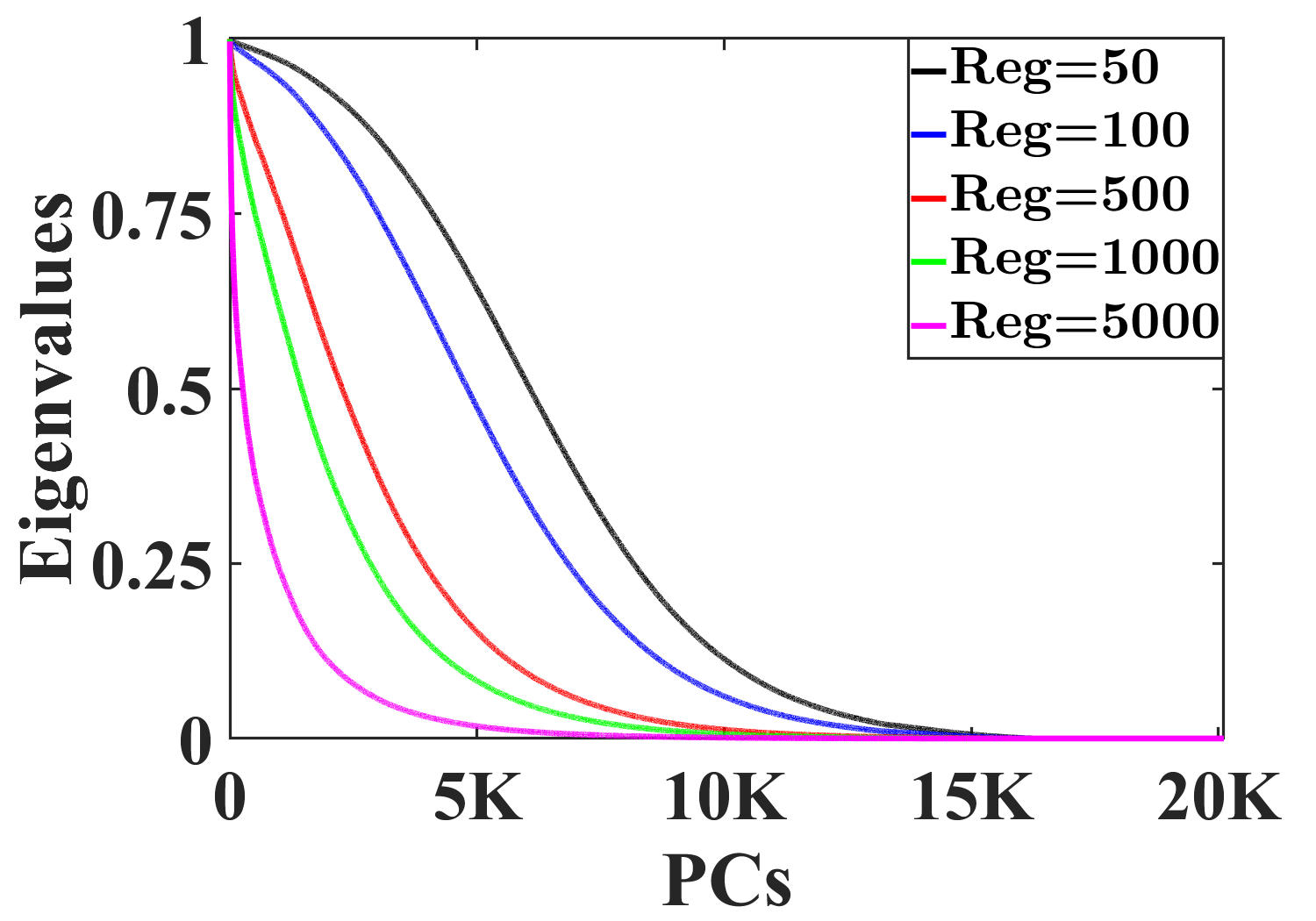
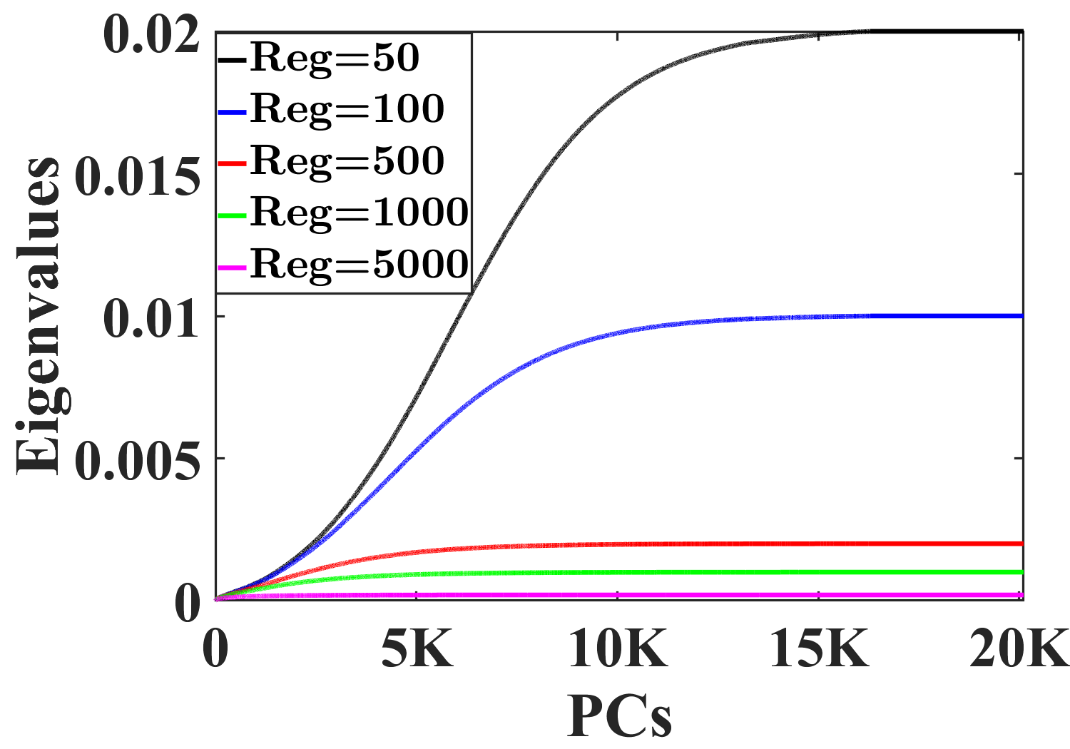
(a) L2 regularization	(b) Diagonal constraints

Figure 1. Distribution of eigenvalues scaled by (a) the L2 regularization $\left(\boldsymbol{\Sigma}^{\top}\boldsymbol{\Sigma}+\lambda\mathbf{I}\right)^{-1}\left(\boldsymbol{\Sigma}^{\top}\boldsymbol{\Sigma}\right)$ and (b) the zero-diagonal constraints $\left(\boldsymbol{\Sigma}^{\top}\boldsymbol{\Sigma}+\lambda\mathbf{I}\right)^{-1}$ on the ML-20M dataset with various $\lambda$.

We then compare the eigenvalues of two terms: the L2 regularization and the zero-diagonal constraints. Figure 1 depicts the distribution of eigenvalues scaled by each term on the ML-20M dataset. The former is represented by the function of $\sigma_{i}^{2}/(\sigma_{i}^{2}+\lambda)$, and the latter is represented by $1/(\sigma_{i}^{2}+\lambda)$ depending on $\sigma_{i}^{2}$ and $\lambda$. In Figure 1(a), the eigenvalue of the L2 regularization ranges from $[0,1]$. Assuming that $\sigma_{1}^{2}>\cdots>\sigma_{n}^{2}$, we observe that (i) the L2 regularization tends to be biased toward high-ranked principal components (PCs). (ii) As $\lambda$ increases, this tendency is strengthened, implying that high-ranked PCs highly influence $\hat{\mathbf{B}}_{LAE}$. We also find interesting observations in Figure 1(b). In contrast to the L2 regularization, the eigenvalue of the diagonal constraints increases as $i$ goes high and ranges from $[0,1/\lambda]$. This observation shows (i) the zero-diagonal constraints tend to emphasize low-ranked PCs. Since it has a negative sign, it penalizes the low-ranked PCs in the solution. (ii) As $\lambda$ increases, this tendency weakens, implying that the impact of L2 regularization dominates the zero-diagonal constraint. In other words, the gap between $\hat{\mathbf{B}}_{LAE}$ and $\hat{\mathbf{B}}_{EASE^{R}}$ diminishes as $\lambda$ increases.

Our analyses can be extended to DLAE and EDLAE. The regularization term is replaced by $\text{diag}(\boldsymbol{\Lambda})=(\lambda_{1},\ldots,\lambda_{n})$, where $\lambda_{i}\neq\lambda_{j}$. By following the same procedure as Eqs. (14) and (16), $\hat{\mathbf{B}}_{DLAE}$ and the zero-diagonal constraints in $\hat{\mathbf{B}}_{EDLAE}$ can also be rewritten as follows, respectively.

(18) $$\begin{split}\hat{\mathbf{B}}_{DLAE}&=\left(\mathbf{X}^{\top}\mathbf{X}+\boldsymbol{\Lambda}\right)^{-1}\left(\mathbf{X}^{\top}\mathbf{X}\right)\\ &=\mathbf{V}\left(\left(\boldsymbol{\Sigma}^{\top}\boldsymbol{\Sigma}\right)+\mathbf{V}^{\top}\boldsymbol{\Lambda}\mathbf{V}\right)^{-1}\left(\boldsymbol{\Sigma}^{\top}\boldsymbol{\Sigma}\right)\mathbf{V}^{\top}\\ \end{split}$$

(19) $$\begin{split}\hat{\mathbf{B}}_{EDLAE}-\hat{\mathbf{B}}_{DLAE}&=-\left(\mathbf{X}^{\top}\mathbf{X}+\boldsymbol{\Lambda}\right)^{-1}\text{diagMat}\left(\boldsymbol{\mu}\right)\\ &=-\mathbf{V}\left(\left(\boldsymbol{\Sigma}^{\top}\boldsymbol{\Sigma}\right)+\mathbf{V}^{\top}\boldsymbol{\Lambda}\mathbf{V}\right)^{-1}\mathbf{V}^{\top}\text{diagMat}\left(\boldsymbol{\mu}\right)\\ \end{split}$$

Although the forms are similar to LAE and EASE^R, we cannot further simplify $\mathbf{V}^{\top}\boldsymbol{\Lambda}\mathbf{V}$ in $\left(\left(\boldsymbol{\Sigma}^{\top}\boldsymbol{\Sigma}\right)+\mathbf{V}^{\top}\boldsymbol{\Lambda}\mathbf{V}\right)^{-1}$ because the commutative law between $\boldsymbol{\Lambda}$ and $\mathbf{V}$ does not always hold, $\mathbf{V}^{\top}\boldsymbol{\Lambda}\mathbf{V}\neq\boldsymbol{\Lambda}$. Thus, it is non-trivial to analyze DLAE and EDLAE with different regularization values in $\boldsymbol{\Lambda}$. Note that our analyses differ from those of the low-rank regression models in (Jin et al., 2021). (We claim the formula expansions in (Jin et al., 2021) are incorrect.)

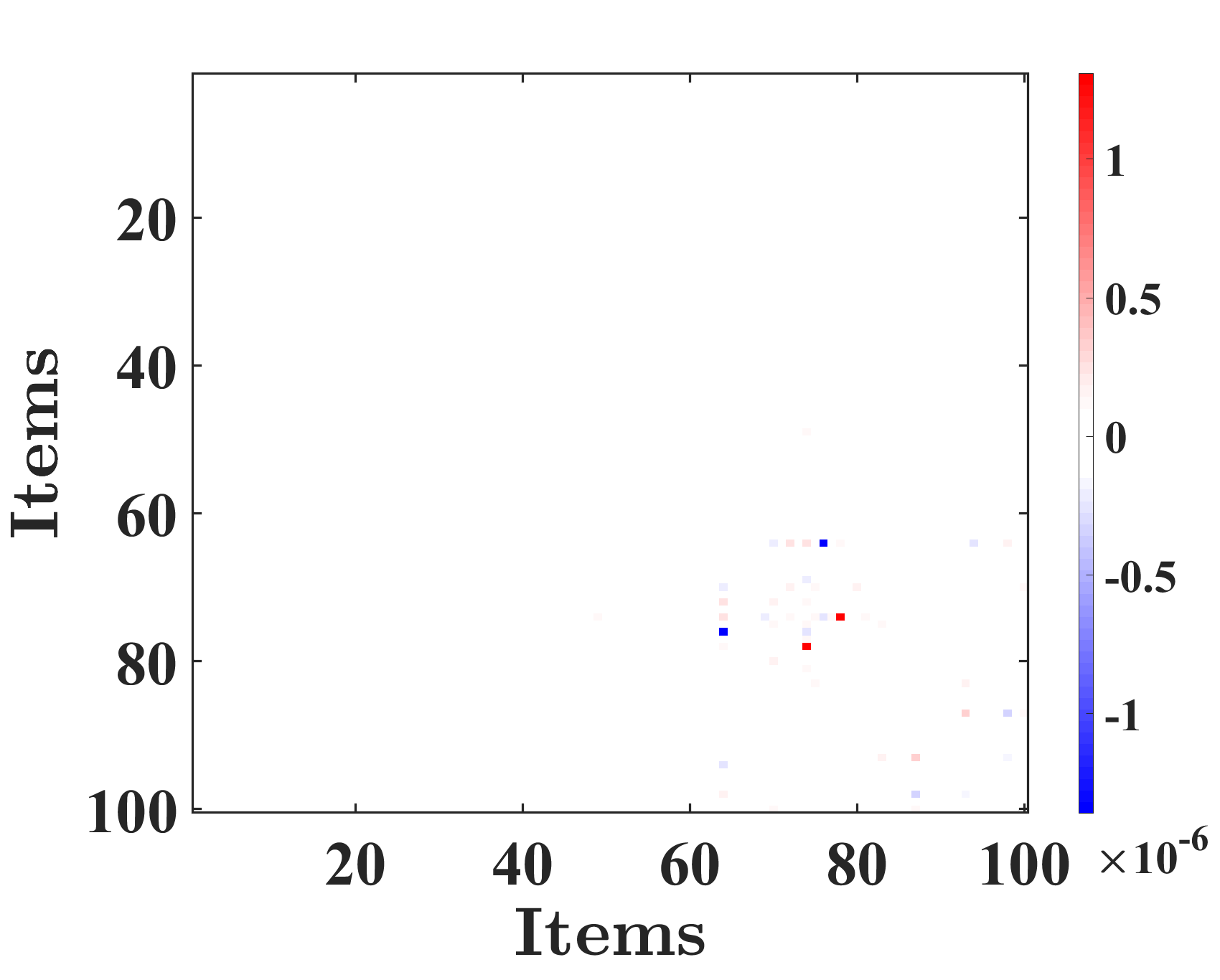
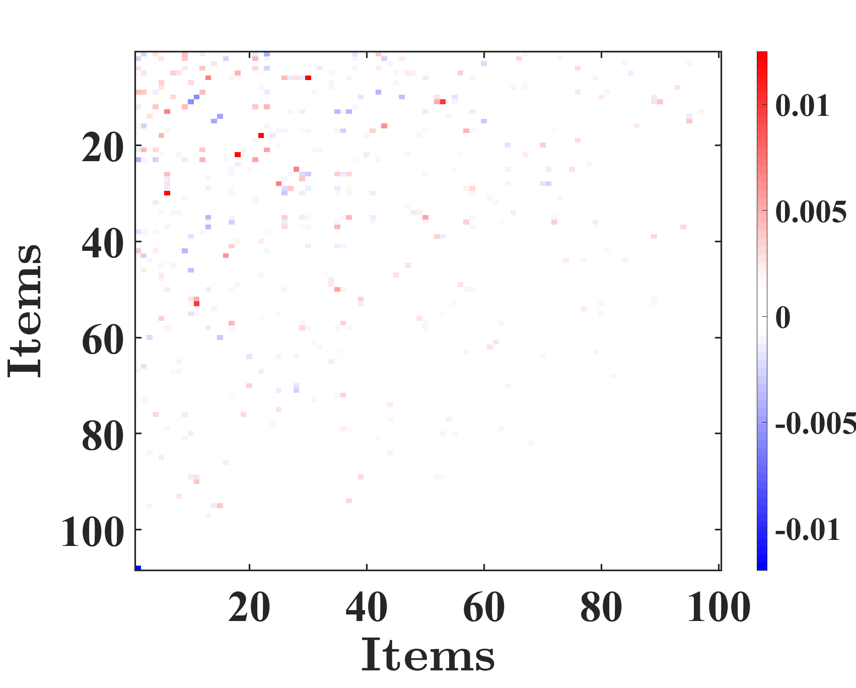
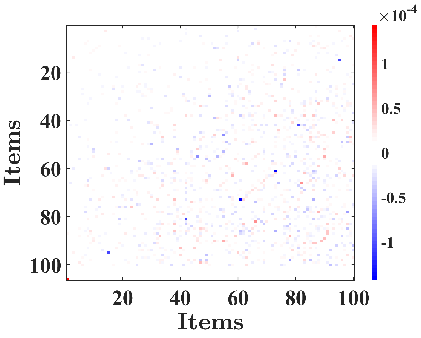
(a) High-ranked PCs	(b) Low-ranked PCs

Figure 2. Visualization of (a) high-ranked PCs and (b) low-ranked PCs of LAE solution, on two datasets (Top: ML-20M, Bottom: Yelp2018). Among 100 items, the first 20 items are popular, and the remaining 80 are unpopular. Items are sorted by popularity.

We further analyze the effects of L2 regularization and diagonal constraints on recommendations in terms of item popularity. Since the gram matrix is represented by an eigenvalue decomposition form, we utilize principal component analysis (PCA). Assuming that $\sigma_{1}^{2}>\cdots>\sigma_{n}^{2}$, the high-ranked PCs contain strong collaborative signals. Since popular items have more chances to co-occur, they are closely related to high-ranked PCs. Meanwhile, low-ranked PCs capture weak collaborative signals.

We conduct a pilot study to better understand the difference between two PC groups (high vs. low) by analyzing Eq. (15). Figure 2(a) and (b) visualize the high-ranked and low-ranked PCs, respectively, on the ML-20M and Yelp2018 datasets. We choose the top 20% and bottom 20% of PCs as two groups and then aggregate them with a weighted sum, using their corresponding eigenvalues as coefficients. For simplicity, we visualize only 100 items randomly drawn from each group, i.e., 20 for popular and 80 for unpopular groups.

On the ML-20M dataset, high-ranked PCs represent the collaborative signals between popular items, while low-ranked PCs represent the correlation between unpopular items (top of Figure 2). In other words, item popularity is highly related to the order of PCs regardless of the magnitude of eigenvalues. However, the trends on Yelp2018 are quite different from ML-20M (bottom of Figure 2). Since the item popularity bias of Yelp2018 is relatively lower than that of ML-20M, both high- and low-ranked PCs have a spread collaborative signal. Therefore, low-ranked PCs are likely to represent weak yet informative collaborative signals.

Based on this analysis, we discuss the effects of L2 regularization and zero-diagonal constraints. (i) L2 regularization mainly considers high-ranked PCs, implying that it removes weak collaborative signals. As $\lambda$ increases, it captures only strong collaborative signals and tends to recommend popular items. Notably, huge $\lambda$ provides only popularity-based recommendation results when the dataset is highly skewed to popular items. (ii) The zero-diagonal constraints mostly penalize low-ranked PCs, eliminating the weak collaborative signals (for the modest $\lambda$). When popular items dominate collaborative signals, using zero-diagonal constraints reduces weak collaborative signals and interrupts the recommendation of less popular items. As a result, it hinders the performance of long-tail recommendations.

4. Relaxing Diagonal Constraints

In this section, we propose novel linear autoencoder models via diagonal constraints relaxation, called Relaxed Linear AutoEncoder (RLAE). First, we formulate the convex optimization problem of RLAE using diagonal inequality constraints and derive the solution of RLAE. We then analyze the relationship between RLAE and other linear autoencoder models, i.e., LAE and EASE^R. Our mathematical analysis shows that RLAE is a generalized version of linear autoencoder models with diagonal constraints.

4.1. Convex Optimization Problem

The convex optimization problem of RLAE is formulated by relaxing the diagonal constraints in Eq. (4).

(20) $$\min_{\mathbf{B}}\|\mathbf{X}-\mathbf{X}\mathbf{B}\|_{F}^{2}+\lambda\|\mathbf{B}\|_{F}^{2}\ \ s.t.\ \ \text{diag}(\mathbf{B})\leq\xi,$$

where $\xi$ is the hyperparameter for relaxing diagonal constraints. When $\xi=0$, it is equivalent to zero-equality constraints, implying EASE^R. If there are no diagonal constraints, i.e., $\xi\geq 1$, then RLAE is induced to LAE. (In Section 4.2, we prove the relation of RLAE to other linear models by controlling the $\xi$.)

RLAE still achieves a closed-form solution via Karush–Kuhn–Tucker (KKT) conditions. Surprisingly, the solution form of RLAE is equivalent to that of EASE^R.

(21) $$\begin{split}\hat{\mathbf{B}}_{RLAE}&=\left(\mathbf{X}^{\top}\mathbf{X}+\lambda\mathbf{I}\right)^{-1}\left(\mathbf{X}^{\top}\mathbf{X}-\text{diagMat}(\boldsymbol{\mu})\right)\\ &=\mathbf{I}-\mathbf{P}\cdot\text{diagMat}(\lambda+\boldsymbol{\mu}),\end{split}$$

(22) $$\text{where}\ {\mu}_{j}= \begin{cases}\ \ \ 0&\text{if}\ \ \ 1-\mathbf{P}_{jj}\lambda\leq\xi,\\ \ \ \ \frac{1-\xi}{\mathbf{P}_{jj}}-\lambda&\text{otherwise}.\end{cases}$$

The key difference is that the diagonal vector $\boldsymbol{\mu}$ is determined by the inequality condition, i.e., $1-\mathbf{P}_{jj}\lambda\leq\xi$. If the inequality condition is satisfied, it becomes 0, i.e., $\mu_{j}=0$. Otherwise, $\mu_{j}$ is equal to $\frac{1-\xi}{\mathbf{P}_{jj}}-\lambda$, relaxing the equality constraints by $\xi$. That is, the diagonal constraints are controlled by $\xi$.

We can also modify the convex optimization problem of DLAE by applying the diagonal inequality constraints. We call it Relaxed Denoising Linear AutoEncoder (RDLAE).

(23) $$\min_{\mathbf{B}}\|\mathbf{X}-\mathbf{X}\mathbf{B}\|_{F}^{2}+\|\boldsymbol{\Lambda}^{1/2}\cdot\mathbf{B}\|_{F}^{2}\ \ s.t.\ \ \text{diag}(\mathbf{B})\leq\xi,\\$$

where $\boldsymbol{\Lambda}=\frac{p}{1-p}\cdot\text{diagMat}\left(\text{diag}(\mathbf{X}^{\top}\mathbf{X})\right)+\lambda\mathbf{I}$.

Also, the solution of RDLAE can be formulated by the closed-form equation. Let $\mathbf{P}^{\prime}=\left(\mathbf{X}^{\top}\mathbf{X}+\boldsymbol{\Lambda}\right)^{-1}$, then the optimization problem Eq. (23) yields the following solution.

(24) $$\begin{split}\hat{\mathbf{B}}_{RDLAE}&=\left(\mathbf{X}^{\top}\mathbf{X}+\boldsymbol{\Lambda}\right)^{-1}\left(\mathbf{X}^{\top}\mathbf{X}-\text{diagMat}(\boldsymbol{\mu})\right)\\ &=\mathbf{I}-\mathbf{P}^{\prime}\cdot\text{diagMat}\left(\text{diag}(\Lambda)+\boldsymbol{\mu}\right),\end{split}$$

(25) $$\text{where}\ {\mu}_{j}= \begin{cases}\ \ \ 0&\text{if}\ \ \ 1-\mathbf{P}^{\prime}_{jj}\Lambda_{j}\leq\xi,\\ \ \ \ \frac{1-\xi}{\mathbf{P}^{\prime}_{jj}}-\Lambda_{j}&\text{otherwise}.\end{cases}$$

4.2. Upper and Lower Bounds Analysis of $\xi$

In this subsection, we show that RDLAE is a generalized version of two linear models, DLAE and EDLAE. We prove the upper and lower bounds of $\xi$. Note that our proof is also used for RLAE since it is a special case without using dropout, i.e., $p=0$.

Theorem 4.1.

If $\xi\geq 1$, the solution of RDLAE is equivalent to that of DLAE.

Proof.

The condition for $\mu_{j}$ to be zero is as follows.

(26) $$1-\mathbf{P}^{\prime}_{jj}\boldsymbol{\Lambda}_{jj}\leq\xi\ \Leftrightarrow\ \mathbf{P}^{\prime}_{jj}\boldsymbol{\Lambda}_{jj}\geq 1-\xi$$

We will show that all diagonal entries of $\mathbf{P}^{\prime}\boldsymbol{\Lambda}$ must be greater than or equal to zero. If a real-valued matrix is positive definite, then all diagonal entries are positive (Harville, 1998). $(\mathbf{X}^{\top}\mathbf{X}+\boldsymbol{\Lambda})$ is positive definite because all diagonal entries of $\boldsymbol{\Lambda}$ are positive (Harville, 1998; Hoerl and Kennard, 2000; Steck, 2020). Since the inverse of the positive definite matrix is a positive definite matrix, $\mathbf{P}^{\prime}=(\mathbf{X}^{\top}\mathbf{X}+\boldsymbol{\Lambda})^{-1}$ is also positive definite. Therefore, the diagonal entries $\mathbf{P}^{\prime}_{jj}$ are greater than zero for all $j$. Accordingly, if $\xi\geq 1$, the condition (26) is satisfied for all $j$, and thus the Lagrangian multiplier vector $\boldsymbol{\mu}$ becomes a zero vector. As a result, the diagonal constraints of RDLAE are ignored, indicating the solution of DLAE. ∎

Theorem 4.2.

If $\xi=0$, the solution of RDLAE is equivalent to that of EDLAE.

Proof.

In the solution of RDLAE, the condition for the $j$th diagonal entry to be constrained is as follows.

(27) $$1-\mathbf{P}^{\prime}_{jj}\boldsymbol{\Lambda}_{jj}\geq\xi\ \Leftrightarrow\ \mathbf{P}^{\prime}_{jj}\boldsymbol{\Lambda}_{jj}\leq 1-\xi$$

We will show that all diagonal entries of $\mathbf{P}^{\prime}\boldsymbol{\Lambda}={(\mathbf{X}^{\top}\mathbf{X}+\boldsymbol{\Lambda})^{-1}}\boldsymbol{\Lambda}$ must be less than 1. $\mathbf{X}^{\top}\mathbf{X}$ is positive semi-definite, so all diagonal entries are semi-positive, i.e., greater or equal to zero (Harville, 1998). From the proof of Theorem 4.1, $\mathbf{P}^{\prime}=(\mathbf{X}^{\top}\mathbf{X}+\boldsymbol{\Lambda})^{-1}$ is positive definite. Since the matrix multiplication between positive and positive semi-definite matrices yields a positive semi-definite matrix (Harville, 1998), $(\mathbf{X}^{\top}\mathbf{X}+\boldsymbol{\Lambda})^{-1}(\mathbf{X}^{\top}\mathbf{X})=\mathbf{I}-(\mathbf{X}^{\top}\mathbf{X}+\boldsymbol{\Lambda)}^{-1}\boldsymbol{\Lambda}=\mathbf{I}-\mathbf{P}^{\prime}\boldsymbol{\Lambda}$ is positive semi-definite. Since the diagonal entries of $\mathbf{I}-\mathbf{P}^{\prime}\boldsymbol{\Lambda}$ are all semi-positive, $\mathbf{P}^{\prime}_{jj}\boldsymbol{\Lambda}_{jj}$ is less or equal to 1 for all $j$. In other words, the condition (27) is satisfied for all $j$. As a result, all diagonal entries of RDLAE are constrained to be zero, indicating the solution of EDLAE. ∎

5. Experimental Setup

Table 1. Statistics of six benchmark datasets: ML-20M, Netflix, MSD, Gowalla, Yelp2018, and Amazon-book.

Dataset	#Users	#Items	#Ratings	Density	$Gini_{item}$
ML-20M	136,677	20,108	10.0M	0.36%	0.90
Netflix	463,435	17,769	56.9M	0.69%	0.86
MSD	571,355	41,140	33.6M	0.36%	0.56
Gowalla	29,858	40,981	1,027,370	0.01%	0.44
Yelp2018	31,668	38,048	1,561,406	0.13%	0.51
Amazon-book	52,643	91,599	2,984,108	0.06%	0.46

Datasets. We extensively conduct experiments and analyses on six benchmark datasets, such as ML-20M, Netflix, MSD, Gowalla, Yelp2018, and Amazon-book, widely used in existing studies (Wang et al., 2019; He et al., 2020; Choi et al., 2021; Steck, 2019, 2020; Chin et al., 2022). In (Chin et al., 2022), they are categorized into different dataset groups. (i) Gowalla, Yelp2018, and Amazon-book are mainly used to evaluate matrix factorization models due to the characteristics of a relatively small number of users and high sparsity. (ii) Meanwhile, ML-20M, Netflix, and MSD are usually used to evaluate autoencoder models due to a large number of users. For reproducibility, we follow the preprocessing used in (Wang et al., 2019) and (Liang et al., 2018). Table 1 summarizes the statistics of the datasets.

Baseline models. We compare our models with state-of-the-art linear autoencoders, LAE, EASE^R (Steck, 2019), DLAE, and EDLAE (Steck, 2020). We also evaluate the following state-of-the-art CF models.

• GRMF (Rao et al., 2015) is the MF model that enhances the smoothness of embeddings via the graph Laplacian regularizer. Following (He et al., 2020; Choi et al., 2021), we used BPR loss for model training.

• MultVAE (Liang et al., 2018) is the neural autoencoder model using variational inference.

• LightGCN (He et al., 2020) is the neural MF model using simplified graph convolutional networks (GCNs).

• LT-OCF (Choi et al., 2021) is the neural MF model using learnable-time graph convolutional networks (GCNs) in which neural ODE (NODE) is used to find the optimal number of GCN layers.

• GF-CF (Shen et al., 2021) is the linear autoencoder model that combines normalized singular vectors with linear and ideal low-pass filters.

• HMLET (Kong et al., 2022) is the neural MF model using linear and non-linear hybrid graph convolutional networks (GCNs) with gating modules.

Evaluation protocols and metrics: For extensive evaluations, we adopt two evaluation protocols (Liang et al., 2018; Wang et al., 2019). While existing CF models merely employ one of the two protocols, we validate the generalized efficacy of our models on both of them.

• Strong generalization: It randomly holds out a set of 80% users for the training set. The remaining half and the others are used for the validation and test set, respectively. We use weak generalization for the validation and test sets; assuming the user has 80% own ratings, CF models provide top-$N$ recommendation lists for 20% unseen ratings. Because it evaluates unseen users as the test set, it is more applicable to real-world scenarios.

• Weak generalization. According to the conventional protocol (Wang et al., 2019; He et al., 2020; Choi et al., 2021), we randomly split a user-item interaction matrix into 80% training and 20% test matrices.

We use two evaluation metrics, Recall and Normalized Discounted Cumulative Gain (NDCG), widely used in the literature (Liang et al., 2018; Wang et al., 2019; He et al., 2020; Choi et al., 2021). While recall quantifies how many preferred items exist, NDCG accounts for the position of preferred items in the top-$N$ recommendation list. To further analyze linear autoencoders, we adopt Average-Over-All (AOA) and unbiased evaluation (Yang et al., 2018). The unbiased evaluation measures true relevance under the missing-not-at-random (MNAR) assumption, so it helps mitigate the impact of popularity bias. We use $\gamma=2$ as the normalization parameter for unbiased evaluation, which is commonly used in existing studies (Yang et al., 2018; Lee et al., 2022). We also report the results of two item groups, i.e., head and tail items, in terms of AOA evaluation. The head items are the top 20% most popular, and the tail items are the rest.

Reproducibility. We reproduced the experimental results of non-linear baselines using the hyperparameter settings provided in the original papers (He et al., 2020; Choi et al., 2021). We conducted a grid search for linear autoencoder models to find optimal hyperparameters. The L2 regularization coefficient $\lambda$ was searched over $[1,2,\ldots,10,20]$. We searched both the dropout probability $p$ and the inequality threshold $\xi$ in the range of $[0.1,0.2,\ldots,0.9]$. For GF-CF (Shen et al., 2021), $\alpha$ was searched in the range of $[0.0,0.1,\ldots,1.0]$. All the experiments were conducted on a desktop with 2 NVidia A6000, 512 GB memory, and 2 Intel Xeon Gold 6226R (2.90 GHz, 22.53M cache). Our implementations are available at https://github.com/jaewan7599/RDLAE_SIGIR2023.

6. Experimental Results

In this section, we report the experimental results of two evaluation protocols, i.e., strong and weak generalization, on six benchmark datasets against theoretical discussions. Specifically, we address the following research questions:

• (RQ1) Do RLAE and RDLAE effectively provide recommendations that alleviate item popularity bias?

• (RQ2) How do regularization and diagonal constraints in linear autoencoders affect recommendations?

• (RQ3) How much do hyperparameters affect the performance of linear autoencoder models?

Table 2. Performance comparison for the proposed methods and other linear autoencoder models on six datasets with the strong generalization protocol. The best results are marked in bold.

Dataset	Model	AOA				Tail				Unbiased
ML-20M		R@20	N@20	R@100	N@100	R@20	N@20	R@100	N@100	R@20	N@20	R@100	N@100
	GF-CF	0.3250	0.2736	0.5765	0.3570	0.0029	0.0022	0.0111	0.0038	0.2188	0.0371	0.4334	0.0507
	LAE	0.3757	0.3228	0.6277	0.4070	0.0005	0.0001	0.0048	0.0011	0.2827	0.0473	0.5016	0.0606
	EASER	0.3905	0.3390	0.6363	0.4202	0.0052	0.0022	0.0215	0.0056	0.2857	0.0479	0.5113	0.0616
	RLAE	0.3913	0.3402	0.6394	0.4224	0.0137	0.0069	0.0579	0.0167	0.2951	0.0487	0.5283	0.0626
	DLAE	0.3923	0.3408	0.6449	0.4241	0.0084	0.0047	0.0417	0.0120	0.2898	0.0477	0.5251	0.0620
	EDLAE	0.3925	0.3421	0.6410	0.4240	0.0066	0.0035	0.0269	0.0078	0.2859	0.0480	0.5128	0.0619
	RDLAE	0.3932	0.3422	0.6452	0.4252	0.0123	0.0062	0.0524	0.0149	0.2987	0.0489	0.5328	0.0630
Netflix	GF-CF	0.2972	0.2724	0.4973	0.3322	0.0185	0.0123	0.0468	0.0202	0.1868	0.0264	0.3563	0.0358
	LAE	0.3465	0.3237	0.5410	0.3796	0.0066	0.0036	0.0258	0.0087	0.2357	0.0326	0.4068	0.0411
	EASER	0.3618	0.3388	0.5535	0.3938	0.0404	0.0222	0.1093	0.0408	0.2554	0.0351	0.4321	0.0435
	RLAE	0.3623	0.3392	0.5551	0.3945	0.0585	0.0377	0.1342	0.0574	0.2606	0.0355	0.4362	0.0437
	DLAE	0.3621	0.3400	0.5557	0.3950	0.0597	0.0381	0.1320	0.0575	0.2549	0.0355	0.4302	0.0438
	EDLAE	0.3659	0.3428	0.5583	0.3978	0.0470	0.0279	0.1141	0.0461	0.2569	0.0358	0.4328	0.0441
	RDLAE	0.3661	0.3431	0.5588	0.3982	0.0545	0.0344	0.1228	0.0527	0.2598	0.0360	0.4350	0.0443
MSD	GF-CF	0.2513	0.2457	0.4310	0.3111	0.1727	0.1331	0.2978	0.1695	0.2137	0.0282	0.3658	0.0351
	LAE	0.2848	0.2740	0.4778	0.3448	0.1862	0.1234	0.3715	0.1765	0.2568	0.0320	0.4411	0.0401
	EASER	0.3338	0.3261	0.5074	0.3899	0.2504	0.1758	0.4109	0.2232	0.3019	0.0377	0.4663	0.0448
	RLAE	0.3338	0.3261	0.5074	0.3899	0.2507	0.1767	0.4110	0.2240	0.3021	0.0378	0.4664	0.0449
	DLAE	0.3288	0.3208	0.5103	0.3873	0.2526	0.1863	0.4107	0.2325	0.2993	0.0378	0.4666	0.0450
	EDLAE	0.3336	0.3258	0.5124	0.3913	0.2503	0.1782	0.4105	0.2253	0.3014	0.0378	0.4684	0.0450
	RDLAE	0.3341	0.3265	0.5110	0.3914	0.2511	0.1784	0.4109	0.2255	0.3022	0.0379	0.4680	0.0450
Gowalla	GF-CF	0.2252	0.1660	0.4529	0.2318	0.1151	0.0591	0.2962	0.1049	0.1734	0.0343	0.3864	0.0508
	LAE	0.2271	0.1706	0.4491	0.2346	0.0799	0.0371	0.2680	0.0836	0.1672	0.0326	0.3763	0.0487
	EASER	0.2414	0.1831	0.4493	0.2437	0.0941	0.0428	0.2862	0.0909	0.1753	0.0335	0.3802	0.0491
	RLAE	0.2448	0.1873	0.4499	0.2468	0.1243	0.0625	0.3177	0.1113	0.1912	0.0370	0.3922	0.0522
	DLAE	0.2495	0.1891	0.4615	0.2507	0.1109	0.0532	0.3087	0.1026	0.1881	0.0366	0.3965	0.0524
	EDLAE	0.2469	0.1859	0.4619	0.2484	0.0951	0.0432	0.2904	0.0918	0.1790	0.0344	0.3896	0.0504
	RDLAE	0.2499	0.1900	0.4594	0.2510	0.1210	0.0587	0.3173	0.1079	0.1923	0.0373	0.3976	0.0528
Yelp2018	GF-CF	0.1134	0.0900	0.2858	0.1487	0.0155	0.0078	0.0793	0.0251	0.0685	0.0081	0.2007	0.0150
	LAE	0.1160	0.0954	0.2720	0.1487	0.0086	0.0039	0.0635	0.0187	0.0705	0.0086	0.1914	0.0148
	EASER	0.1144	0.0933	0.2681	0.1458	0.0091	0.0042	0.0684	0.0201	0.0679	0.0081	0.1883	0.0143
	RLAE	0.1173	0.0968	0.2726	0.1499	0.0127	0.0060	0.0784	0.0237	0.0735	0.0089	0.1972	0.0152
	DLAE	0.1190	0.0971	0.2784	0.1516	0.0121	0.0057	0.0773	0.0236	0.0724	0.0087	0.1986	0.0152
	EDLAE	0.1171	0.0957	0.2757	0.1499	0.0103	0.0049	0.0727	0.0219	0.0698	0.0084	0.1939	0.0147
	RDLAE	0.1190	0.0976	0.2773	0.1519	0.0161	0.0077	0.0882	0.0274	0.0741	0.0089	0.2018	0.0154
Amazon-book	GF-CF	0.1668	0.1492	0.3182	0.2009	0.0988	0.0702	0.2051	0.1000	0.1401	0.0195	0.2740	0.0263
	LAE	0.1920	0.1749	0.3239	0.2198	0.1012	0.0635	0.2218	0.0980	0.1644	0.0220	0.2896	0.0281
	EASER	0.1912	0.1734	0.3258	0.2193	0.0761	0.0444	0.1815	0.0746	0.1481	0.0195	0.2725	0.0256
	RLAE	0.1968	0.1804	0.3288	0.2255	0.1057	0.0672	0.2260	0.1018	0.1649	0.0221	0.2909	0.0282
	DLAE	0.1994	0.1820	0.3374	0.2291	0.0993	0.0631	0.2187	0.0972	0.1637	0.0220	0.2938	0.0283
	EDLAE	0.1940	0.1756	0.3349	0.2240	0.0829	0.0512	0.1938	0.0827	0.1523	0.0205	0.2820	0.0268
	RDLAE	0.2011	0.1834	0.3354	0.2293	0.1043	0.0670	0.2214	0.1007	0.1663	0.0225	0.2934	0.0286

6.1. Performance Comparison (RQ1, RQ2)

Strong generalization. We compare seven linear models, including GF-CF (Shen et al., 2021), to evaluate the effectiveness of our models. We also perform quantitative analyses of how the regularization and the diagonal constraints affect the performance of linear autoencoder models. Table 2 shows the performance of top-$K$ recommendation on six datasets. Note that we observe similar trends between head items and AOA metrics in the ML-20M, Netflix, and MSD datasets, so we do not report the performance for head items in Table 2.

As shown in Table 2, our models, i.e., RLAE and RDLAE, consistently outperform other linear autoencoder models in both AOA and unbiased evaluation on all six datasets, more significantly in the latter. RLAE and RDLAE show performance gains in the unbiased evaluation of 1.62% and 1.61% on NDCG@100 for the ML-20M dataset, respectively, and 2.70% and 1.32% for the Yelp2018 dataset, respectively. The significant enhancement in tail items drives the improvement in unbiased evaluation, indicating that they can adequately mitigate the popularity bias. Specifically, RLAE and RDLAE show performance gains of 198.21% and 24.17% in tail items on NDCG@100 for the ML-20M dataset, and 17.91% and 16.10% for the Yelp2018 dataset, respectively.

Our models outperform GF-CF, a state-of-the-art model, in almost all metrics. On the three datasets, ML-20M, Netflix, and MSD, RLAE outperforms GF-CF by an average of 20.80% in AOA evaluation, 185.26% in tail items, and 24.49% in unbiased evaluation on NDCG@100. For the strong generalization datasets, using the precision matrix rather than the covariance matrix is better (Steck, 2019). However, the linear filter, one of the main components of GF-CF, is similar to the concept of a covariance matrix, leading to lower performance of GF-CF. On the rest of the datasets, Gowalla, Yelp2018, and Amazon-book, RLAE outperforms GF-CF by an average of 6.47% in AOA evaluation, 0.66% in tail items, and 3.77% in unbiased evaluation on NDCG@100. The ideal low-pass filter, another main component of GF-CF, emphasizes high-ranked PCs but needs to fully account for informative CF signals from low-ranked PCs in these datasets, causing RLAE to outperform GF-CF.

We observe that the popularity bias of the dataset has a significant impact on determining the utility of the diagonal constraint. On the datasets with large popularity bias, i.e., ML-20M, Netflix, and MSD datasets, EASE^R outperforms LAE on all metrics, with an average performance gain of 268.17% in tail items on NDCG@100. Here, the diagonal constraints help models focus on high-ranked PCs, preventing a large increase in L2 regularization. We find that the optimal $\lambda$ for LAE relative to EASE^R is 12.5, 40, and 40 times larger for the three datasets, respectively. This makes unpopular items almost uninformative, resulting in the dramatic performance drop in tail items of LAE.

On the other hand, on the datasets with relatively low popularity bias, such as Gowalla, Yelp2018, and Amazon-book datasets, LAE performs slightly worse or even better than EASE^R. For these datasets, we observe that the optimal $\lambda$ tends to be lower, and the differences between the optimal $\lambda$s of the two models are reduced to a range of less than a factor of two or less. This low $\lambda$ takes into account the relatively uniform importance of PCs’ rank and allows the model to make recommendations based on CF signals from low-ranked PCs as well as high-ranked PCs. In other words, low-ranked PCs are informative in these datasets, and the diagonal constraints that penalize them cause performance degradation. Specifically, LAE outperforms EASE^R by 31.37% in tail items on NDCG@100 for the Amazon-book dataset, even though LAE has a 25% higher $\lambda$ than EASE^R.

Table 3. Performance comparison for linear autoencoder models and deep learning baseline models on Gowalla, Yelp2018, and Amazon-book datasets with the weak generalization protocol. The best results are marked in bold, and the second best models are underlined.

Dataset	Gowalla		Yelp2018		Amazon-Book
Method	R@20	N@20	R@20	N@20	R@20	N@20
GRMF	0.1477	0.1205	0.0571	0.0462	0.0354	0.0270
GRMF-Norm	0.1557	0.1261	0.0561	0.0454	0.0352	0.0269
Mult-VAE	0.1641	0.1335	0.0584	0.0450	0.0407	0.0315
LightGCN	0.1830	0.1554	0.0649	0.0530	0.0411	0.0315
LT-OCF	0.1875	0.1574	0.0671	0.0549	0.0442	0.0341
HMLET	0.1874	0.1589	0.0675	0.0557	0.0482	0.0371
GF-CF	0.1849	0.1536	0.0697	0.0571	0.0710	0.0584
LAE	0.1630	0.1295	0.0658	0.0555	0.0746	0.0611
EASER	0.1765	0.1467	0.0657	0.0552	0.0710	0.0566
DLAE	0.1839	0.1533	0.0678	0.0570	0.0751	0.0610
EDLAE	0.1844	0.1539	0.0673	0.0565	0.0711	0.0566
RLAE	0.1772	0.1467	0.0667	0.0562	0.0754	0.0615
RDLAE	0.1845	0.1539	0.0679	0.0569	0.0754	0.0613

We find that dropout leads to an overall performance improvement, with the optimal $\lambda$ tending to decrease because dropout provides additional regularization. The lower $\lambda$ strengthens the model’s concentration on low-ranked PCs, improving performance on unbiased evaluation and tail items. Specifically, on the ML-20M dataset, where the $\lambda$ of DLAE is reduced by 10 times compared to LAE’s, DLAE significantly outperforms LAE by 900.91% in tail items on NDCG@100, while on the Amazon-book dataset, where the reduction in $\lambda$ is relatively small, DLAE performs slightly worse than LAE with the performance degradation of 0.82%.

Moreover, we observe that the tendency of the diagonal constraints is maintained regardless of whether dropout is applied, but its effectiveness is reduced. For example, on the Netflix and MSD datasets, EASE^R outperforms LAE with a dramatic performance gain, while EDLAE is slightly better than DLAE. Furthermore, EDLAE performs slightly worse than DLAE on the ML-20M dataset. This is because dropout emphasizes high-ranked PCs similarly to diagonal constraints, and we discuss this in Section 6.2.

Weak generalization. Table 3 reports the results of weak generalization by comparing linear autoencoder and neural models. Note that existing studies rarely evaluate linear autoencoder models in this setting.

Our models, i.e., RLAE and RDLAE, still show higher or comparable overall performance compared to other linear autoencoder models in weak generalization. RDLAE is comparable to GF-CF on Gowalla, worse on Yelp2018, and considerably better on Amazon-book on Recall@20. Specifically, for the Amazon-book dataset, RDLAE outperforms GF-CF by 6.20% and 5.31% on Recall@20 and NDCG@20, respectively. In addition, reducing the diagonal constraints helps improve performance on datasets with a low popularity bias. For the Yelp2018 and the Amazon-book datasets, the models with zero-diagonal constraints, i.e., EASE^R and EDLAE, show the worst performance. However, on Gowalla, introducing diagonal constraints offers better performance. Due to the high sparsity, low-ranked PCs in Gowalla may contain noisy information.

We highlight the comparison between RDLAE and HMLET (Kong et al., 2022), a state-of-the-art GCN model. HMLET performs better than RDLAE on the Gowalla dataset. However, as the dataset grows, the performance gain of RDLAE increases. Especially for the Amazon-Book dataset, the largest of the three datasets, RDLAE significantly outperforms HMLET with a 56.43% gain on Recall@20. This is because most neural models are optimized for small datasets rather than large ones. The high sparsity of the dataset also hinders their performance. Meanwhile, linear autoencoders easily capture significant collaborative signals using the closed-form solution regardless of data sparsity.

6.2. Hyperparameter Sensitivity Analysis (RQ3)

To analyze the impact of the hyperparameters, we report the results on the strong generalization protocol for two datasets, ML-20M and Yelp2018. NDCG@100 is used as the default metric. In Figures 3 and 5, we fix the L2 regularization coefficient $\lambda$ to 100. Note that the same trend is shown in other metrics and $\lambda$.

Diagonal constraints. Figure 3 shows the performance of RLAE over varying $\xi$. As $\xi$ goes down, the impact of the diagonal constraints becomes stronger. In particular, $\xi=0$ indicates the zero-diagonal constraints, meaning that the diagonal constraints are applied to all items. The best performance is shown at a specific $\xi$ value, higher than when the zero-diagonal constraints are applied on both datasets. In addition, the performance of the tail items gradually improves as the $\xi$ value increases. This observation implies that the diagonal constraints suppress the collaborative signals of unpopular items. Moreover, we observe that the diagonal constraints do not affect most items at the optimal $\xi$ value. Specifically, RLAE removes 81.31% and 78.76% of the diagonal constraints on the ML-20M and Yelp2018 datasets, respectively.

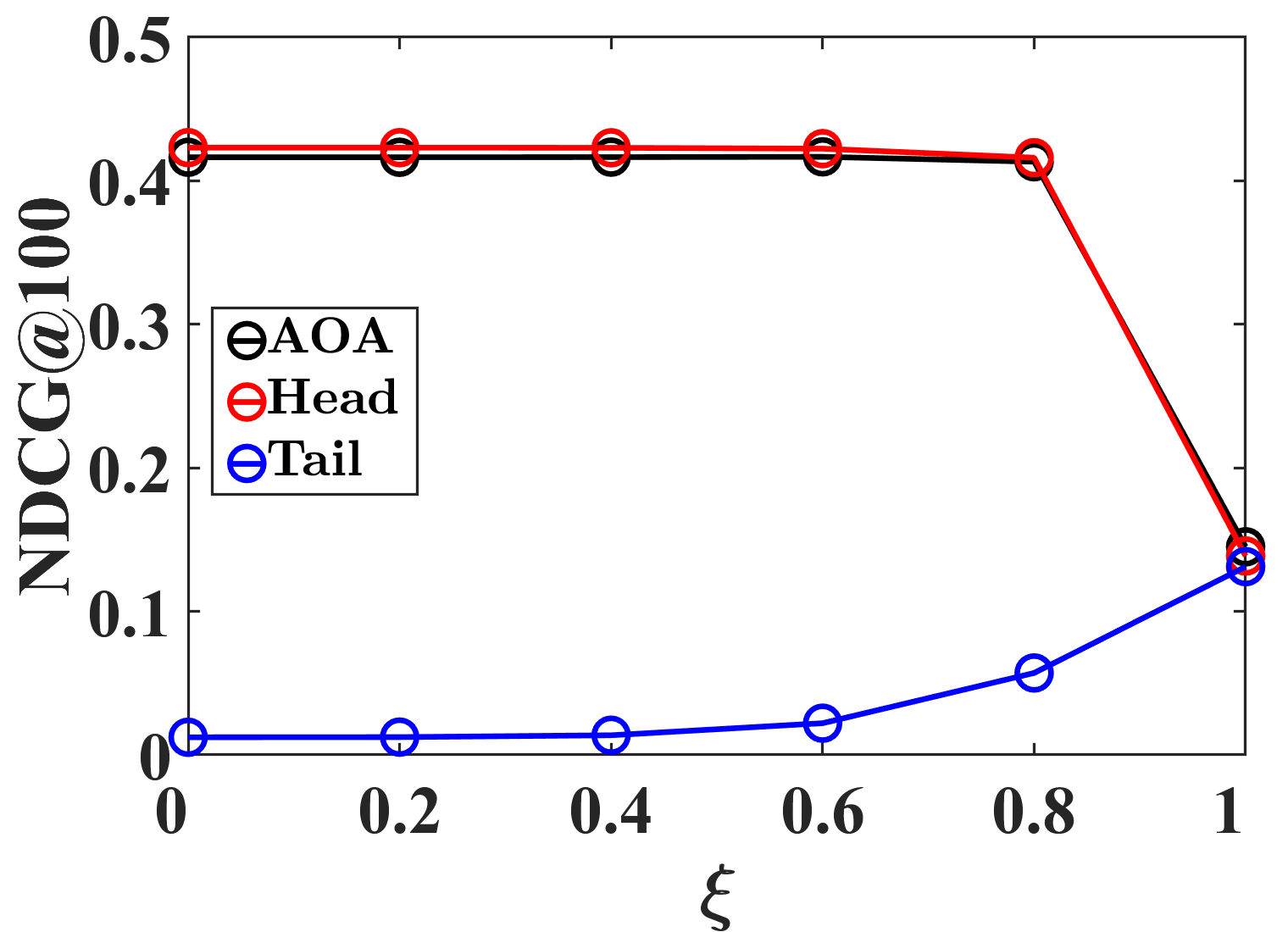
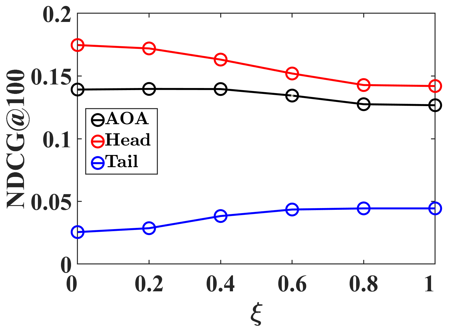
(a) ML-20M	(b) Yelp2018

Figure 3. NDCG@100 of RLAE over various $\boldsymbol{\xi}$ for diagonal constraints on two datasets, ML-20M and Yelp2018.

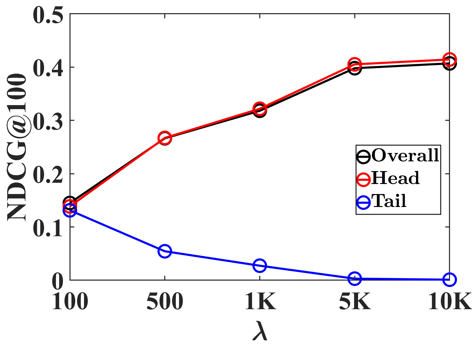
(a) ML-20M	(b) Yelp2018

Figure 4. NDCG@100 of LAE over various $\boldsymbol{\lambda}$ for L2 regularization on two datasets, ML-20M and Yelp2018.

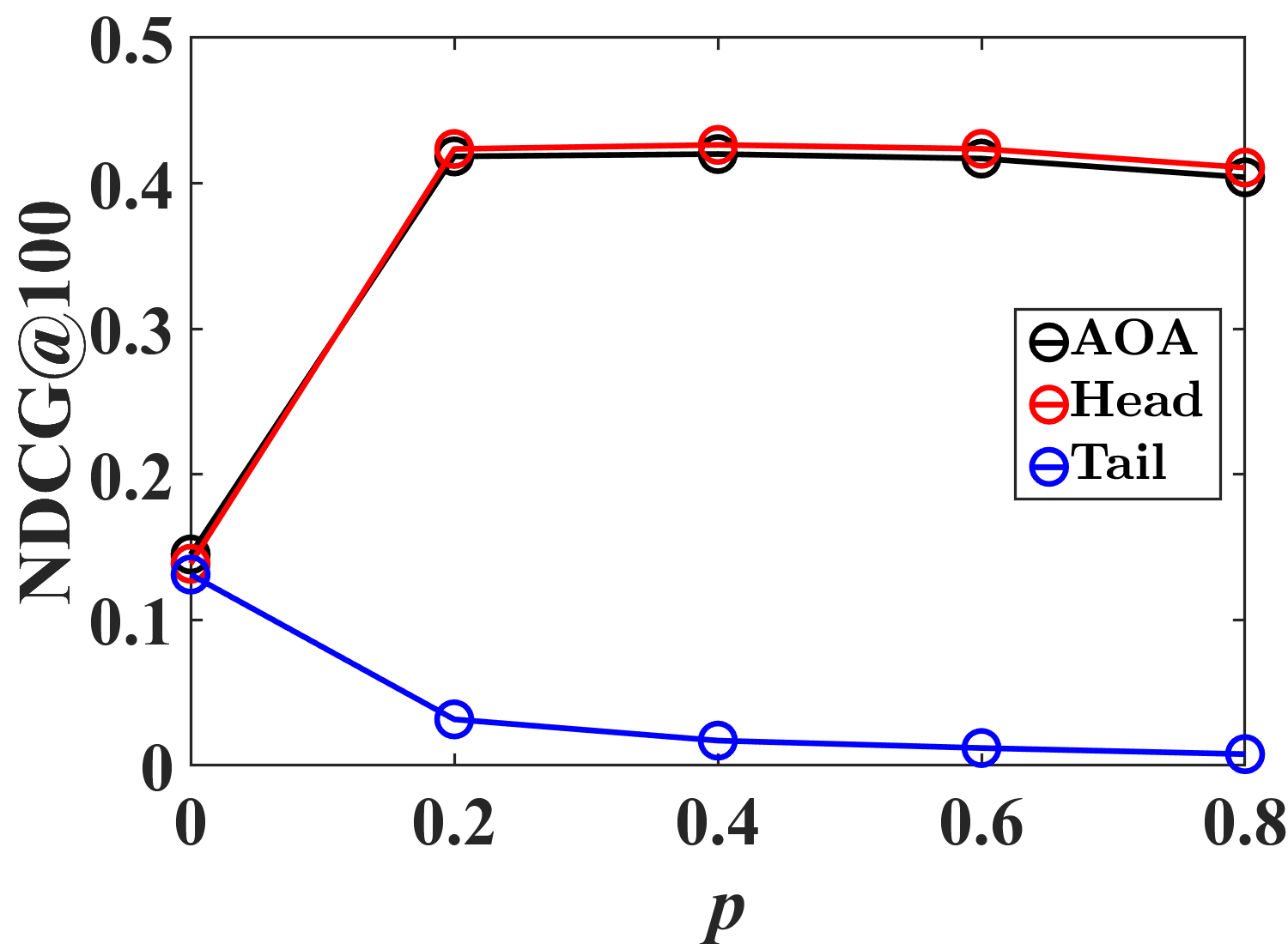
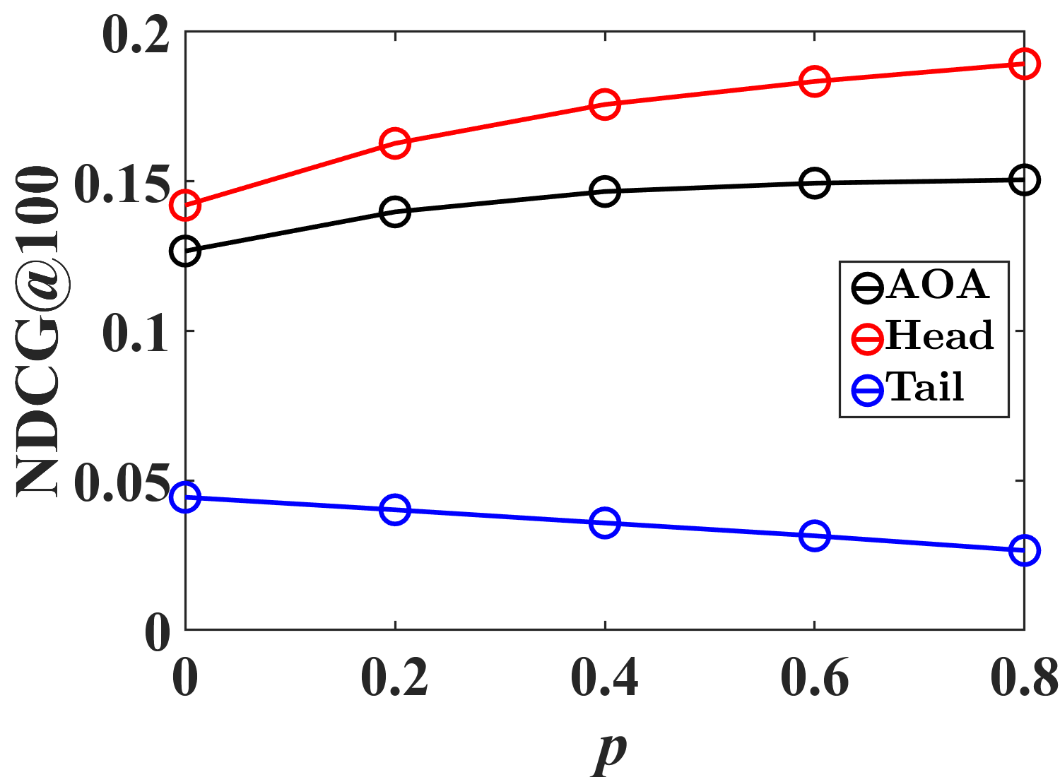
(a) ML-20M	(b) Yelp2018

Figure 5. NDCG@100 of DLAE over various $\mathbf{p}$ for dropout regularization on two datasets, ML-20M and Yelp2018.

L2 regularization. Figure 4 depicts the performance of LAE over various $\lambda$. We use LAE to analyze only the impact of L2 regularization. We highlight the two observations: (1) As $\lambda$ increases, the performance of the head item group tends to increase while the performance of the tail item group tends to decrease. Therefore, it is necessary to adjust the modest L2 regularization to consider the performance balance of both item groups. (2) $\lambda=10K$ shows the best performance on the ML-20M dataset, but the best performance is shown at $\lambda=500$ on the Yelp2018 dataset. Due to the relatively low popularity bias, low-ranked PCs contain more meaningful information on Yelp2018, resulting in the best performance at relatively low $\lambda$. In brief, the optimal value of $\lambda$ depends on the popularity bias.

Dropout regularization. Figure 5 shows the performance of DLAE over varying dropout ratio $p$. We observe similar trends for dropout and diagonal constraints. As the $p$ increases, the performance of head items tends to increase while the performance of tail items consistently decreases for both datasets. Moreover, we observe a correlation between the popularity bias of the dataset and the value of optimal $p$. The larger the item popularity bias, the stronger the impact of dropout regularization. Thus, the variation of performance with $p$ on the ML-20M dataset is more sensitive, with optimal performance occurring at a relatively low $p$ compared to the Yelp2018 dataset.

7. Related Work

We briefly review existing CF models into two groups: linear and non-linear. We also discuss theoretical analyses for understanding linear models.

Linear models. They are categorized into two groups, latent factor models and neighborhood-based models. Latent factor models (Hu et al., 2008; Pan et al., 2008; Zhou et al., 2008; Koren, 2008) factorize an entire matrix into a combination of user and item vectors. Pioneering by (Ning and Karypis, 2011), linear autoencoder models are formulated by the regression model for the item neighborhood-based approach (Sarwar et al., 2001). Recent studies (Steck, 2019; Steck et al., 2020; Jeunen et al., 2020; Steck and Liang, 2021) calculate an item-item weight matrix via convex optimization with L2 regularization and zero-diagonal constraints. Furthermore, EDLAE (Steck, 2020) utilizes advanced regularization derived from random dropout.

Non-linear models. With the blossom of deep learning, non-linear models have been widely used for recommendation. Like linear models, non-linear models are broadly categorized into latent factor models and autoencoder models. Non-linear latent factor models include MF-based neural models (Rendle et al., 2009; He et al., 2017; Rao et al., 2015) and GCN-based models (He et al., 2020; Chen et al., 2020; Wang et al., 2019; Choi et al., 2021; Shen et al., 2021). In addition, non-linear autoencoder models (Wu et al., 2016; Liang et al., 2018; Shenbin et al., 2020; Lobel et al., 2020) utilize a bottleneck architecture consisting of an encoder and a decoder, where the hidden layer represents a non-linear activation function.

Theoretical analysis for linear models. Several studies (Xu et al., 2021; Shen et al., 2021; Jin et al., 2021) have recently conducted in-depth analyses of linear models. (Xu et al., 2021) performed a theoretical analysis on product embedding using skip-gram negative sampling, and (Shen et al., 2021) considered graph signal processing on the GCN-based methodology for the recommendation. In addition, (Jin et al., 2021) compares low-rank linear autoencoders with Tikhonov regularization and a closed-form solution of MF. To the best of our knowledge, no existing study explores diagonal constraints in linear autoencoders.

8. Conclusion

This paper provided a theoretical understanding of linear autoencoder models. Their solutions can be decomposed into two components: an objective function with regularization and zero-diagonal constraints. To the best of our knowledge, no existing study thoroughly investigates the relationship between item popularity and two components of linear autoencoders. Regularization emphasizes high-ranked PCs, affecting strong collaborative signals. Meanwhile, the diagonal constraints weaken the impact of low-ranked PCs. Because low-ranked PCs are highly related to the collaborative signals for unpopular items, the zero-diagonal constraints are not always helpful for enhancing performances, especially for long-tail items. Motivated by our analyses, we suggested linear autoencoder models by relaxing diagonal constraints. Experimental results extensively demonstrated that our models are comparable to or better than existing linear autoencoder and non-linear models using two evaluation protocols on six benchmark datasets.

- (1)
- Chen et al. (2020) Lei Chen, Le Wu, Richang Hong, Kun Zhang, and Meng Wang. 2020. Revisiting Graph Based Collaborative Filtering: A Linear Residual Graph Convolutional Network Approach. In AAAI. 27–34.
- Chin et al. (2022) Jin Yao Chin, Yile Chen, and Gao Cong. 2022. The Datasets Dilemma: How Much Do We Really Know About Recommendation Datasets?. In WSDM. 141–149.
- Choi et al. (2021) Jeongwhan Choi, Jinsung Jeon, and Noseong Park. 2021. LT-OCF: Learnable-Time ODE-based Collaborative Filtering. In CIKM. 251–260.
- Cooper et al. (2014) Colin Cooper, Sang-Hyuk Lee, Tomasz Radzik, and Yiannis Siantos. 2014. Random walks in recommender systems: exact computation and simulations. In WWW. 811–816.
- Dacrema et al. (2021) Maurizio Ferrari Dacrema, Simone Boglio, Paolo Cremonesi, and Dietmar Jannach. 2021. A Troubling Analysis of Reproducibility and Progress in Recommender Systems Research. ACM Trans. Inf. Syst. 39, 2 (2021), 20:1–20:49.
- Dacrema et al. (2019) Maurizio Ferrari Dacrema, Paolo Cremonesi, and Dietmar Jannach. 2019. Are we really making much progress? A worrying analysis of recent neural recommendation approaches. In RecSys. 101–109.
- Goldberg et al. (1992) David Goldberg, David A. Nichols, Brian M. Oki, and Douglas B. Terry. 1992. Using Collaborative Filtering to Weave an Information Tapestry. Commun. ACM 35, 12 (1992), 61–70.
- Harville (1998) David A. Harville. 1998. Matrix algebra from a statistician’s perspective.
- He et al. (2020) Xiangnan He, Kuan Deng, Xiang Wang, Yan Li, Yong-Dong Zhang, and Meng Wang. 2020. LightGCN: Simplifying and Powering Graph Convolution Network for Recommendation. In SIGIR. 639–648.
- He et al. (2017) Xiangnan He, Lizi Liao, Hanwang Zhang, Liqiang Nie, Xia Hu, and Tat-Seng Chua. 2017. Neural Collaborative Filtering. In WWW. 173–182.
- Herlocker et al. (1999) Jonathan L. Herlocker, Joseph A. Konstan, Al Borchers, and John Riedl. 1999. An Algorithmic Framework for Performing Collaborative Filtering. In SIGIR. 230–237.
- Hidasi et al. (2016) Balázs Hidasi, Alexandros Karatzoglou, Linas Baltrunas, and Domonkos Tikk. 2016. Session-based Recommendations with Recurrent Neural Networks. In ICLR.
- Hoerl and Kennard (2000) Arthur E. Hoerl and Robert W. Kennard. 2000. Ridge Regression: Biased Estimation for Nonorthogonal Problems. Technometrics 42, 1 (2000), 80–86.
- Hu et al. (2008) Yifan Hu, Yehuda Koren, and Chris Volinsky. 2008. Collaborative Filtering for Implicit Feedback Datasets. In ICDM. 263–272.
- Jannach et al. (2021) Dietmar Jannach, Pearl Pu, Francesco Ricci, and Markus Zanker. 2021. Recommender Systems: Past, Present, Future. AI Mag. 42, 3 (2021), 3–6.
- Jeunen et al. (2020) Olivier Jeunen, Jan Van Balen, and Bart Goethals. 2020. Closed-Form Models for Collaborative Filtering with Side-Information. In RecSys. 651–656.
- Jin et al. (2021) Ruoming Jin, Dong Li, Jing Gao, Zhi Liu, Li Chen, and Yang Zhou. 2021. Towards a Better Understanding of Linear Models for Recommendation. In KDD. 776–785.
- Kang and McAuley (2018) Wang-Cheng Kang and Julian J. McAuley. 2018. Self-Attentive Sequential Recommendation. In ICDM. 197–206.
- Kong et al. (2022) Taeyong Kong, Taeri Kim, Jinsung Jeon, Jeongwhan Choi, Yeon-Chang Lee, Noseong Park, and Sang-Wook Kim. 2022. Linear, or Non-Linear, That is the Question!. In WSDM. 517–525.
- Koren (2008) Yehuda Koren. 2008. Factorization meets the neighborhood: a multifaceted collaborative filtering model. In KDD. 426–434.
- Lee et al. (2022) Jae-woong Lee, Seongmin Park, Joonseok Lee, and Jongwuk Lee. 2022. Bilateral Self-unbiased Learning from Biased Implicit Feedback. In SIGIR. 29–39.
- Li et al. (2017) Jing Li, Pengjie Ren, Zhumin Chen, Zhaochun Ren, Tao Lian, and Jun Ma. 2017. Neural Attentive Session-based Recommendation. In CIKM. 1419–1428.
- Liang et al. (2018) Dawen Liang, Rahul G. Krishnan, Matthew D. Hoffman, and Tony Jebara. 2018. Variational Autoencoders for Collaborative Filtering. In WWW. 689–698.
- Lobel et al. (2020) Sam Lobel, Chunyuan Li, Jianfeng Gao, and Lawrence Carin. 2020. RaCT: Toward Amortized Ranking-Critical Training For Collaborative Filtering. In ICLR.
- Ning and Karypis (2011) Xia Ning and George Karypis. 2011. SLIM: Sparse Linear Methods for Top-N Recommender Systems. In ICDM. 497–506.
- Pan et al. (2008) Rong Pan, Yunhong Zhou, Bin Cao, Nathan Nan Liu, Rajan M. Lukose, Martin Scholz, and Qiang Yang. 2008. One-Class Collaborative Filtering. In ICDM. 502–511.
- Paudel et al. (2017) Bibek Paudel, Fabian Christoffel, Chris Newell, and Abraham Bernstein. 2017. Updatable, Accurate, Diverse, and Scalable Recommendations for Interactive Applications. ACM Trans. Interact. Intell. Syst. 7, 1 (2017), 1:1–1:34.
- Rao et al. (2015) Nikhil Rao, Hsiang-Fu Yu, Pradeep Ravikumar, and Inderjit S. Dhillon. 2015. Collaborative Filtering with Graph Information: Consistency and Scalable Methods. In NIPS. 2107–2115.
- Rendle et al. (2009) Steffen Rendle, Christoph Freudenthaler, Zeno Gantner, and Lars Schmidt-Thieme. 2009. BPR: Bayesian Personalized Ranking from Implicit Feedback. In UAI. 452–461.
- Rendle et al. (2019) Steffen Rendle, Li Zhang, and Yehuda Koren. 2019. On the Difficulty of Evaluating Baselines: A Study on Recommender Systems. CoRR abs/1905.01395 (2019).
- Sarwar et al. (2001) Badrul Munir Sarwar, George Karypis, Joseph A. Konstan, and John Riedl. 2001. Item-based collaborative filtering recommendation algorithms. In WWW. 285–295.
- Shen et al. (2021) Yifei Shen, Yongji Wu, Yao Zhang, Caihua Shan, Jun Zhang, Khaled B. Letaief, and Dongsheng Li. 2021. How Powerful is Graph Convolution for Recommendation?. In CIKM. 1619–1629.
- Shenbin et al. (2020) Ilya Shenbin, Anton Alekseev, Elena Tutubalina, Valentin Malykh, and Sergey I. Nikolenko. 2020. RecVAE: A New Variational Autoencoder for Top-N Recommendations with Implicit Feedback. In WSDM. 528–536.
- Steck (2019) Harald Steck. 2019. Embarrassingly Shallow Autoencoders for Sparse Data. In WWW. 3251–3257.
- Steck (2020) Harald Steck. 2020. Autoencoders that don’t overfit towards the Identity. In NeurIPS.
- Steck et al. (2020) Harald Steck, Maria Dimakopoulou, Nickolai Riabov, and Tony Jebara. 2020. ADMM SLIM: Sparse Recommendations for Many Users. In WSDM. 555–563.
- Steck and Liang (2021) Harald Steck and Dawen Liang. 2021. Negative Interactions for Improved Collaborative Filtering: Don’t go Deeper, go Higher. In RecSys. 34–43.
- Sun et al. (2019) Fei Sun, Jun Liu, Jian Wu, Changhua Pei, Xiao Lin, Wenwu Ou, and Peng Jiang. 2019. BERT4Rec: Sequential Recommendation with Bidirectional Encoder Representations from Transformer. In CIKM. 1441–1450.
- Sun et al. (2020) Zhu Sun, Di Yu, Hui Fang, Jie Yang, Xinghua Qu, Jie Zhang, and Cong Geng. 2020. Are We Evaluating Rigorously? Benchmarking Recommendation for Reproducible Evaluation and Fair Comparison. In RecSys. 23–32.
- Vancura et al. (2022) Vojtech Vancura, Rodrigo Alves, Petr Kasalický, and Pavel Kordík. 2022. Scalable Linear Shallow Autoencoder for Collaborative Filtering. In RecSys. 604–609.
- Wang et al. (2019) Xiang Wang, Xiangnan He, Meng Wang, Fuli Feng, and Tat-Seng Chua. 2019. Neural Graph Collaborative Filtering. In SIGIR. 165–174.
- Wu et al. (2016) Yao Wu, Christopher DuBois, Alice X. Zheng, and Martin Ester. 2016. Collaborative Denoising Auto-Encoders for Top-N Recommender Systems. In WSDM. 153–162.
- Xu et al. (2021) Da Xu, Chuanwei Ruan, Evren Körpeoglu, Sushant Kumar, and Kannan Achan. 2021. Theoretical Understandings of Product Embedding for E-commerce Machine Learning. In WSDM. 256–264.
- Yang et al. (2018) Longqi Yang, Yin Cui, Yuan Xuan, Chenyang Wang, Serge J. Belongie, and Deborah Estrin. 2018. Unbiased offline recommender evaluation for missing-not-at-random implicit feedback. In RecSys. 279–287.
- Zhou et al. (2008) Yunhong Zhou, Dennis M. Wilkinson, Robert Schreiber, and Rong Pan. 2008. Large-Scale Parallel Collaborative Filtering for the Netflix Prize. In AAIM (Lecture Notes in Computer Science, Vol. 5034). 337–348.