RSA-INR: Riemannian Shape Autoencoding via
4D Implicit Neural Representations

Abstract

Shape encoding and shape analysis are valuable tools for comparing shapes and for dimensionality reduction. A specific framework for shape analysis is the Large Deformation Diffeomorphic Metric Mapping (LDDMM) framework, which is capable of shape matching and dimensionality reduction. Researchers have recently introduced neural networks into this framework. However, these works can not match more than two objects simultaneously or have suboptimal performance in shape variability modeling. The latter limitation occurs as the works do not use state-of-the-art shape encoding methods. Moreover, the literature does not discuss the connection between the LDDMM Riemannian distance and the Riemannian geometry for deep learning literature. Our work aims to bridge this gap by demonstrating how LDDMM can integrate Riemannian geometry into deep learning. Furthermore, we discuss how deep learning solves and generalizes shape matching and dimensionality reduction formulations of LDDMM. We achieve both goals by designing a novel implicit encoder for shapes. This model extends a neural network-based algorithm for LDDMM-based pairwise registration, results in a nonlinear manifold PCA, and adds a Riemannian geometry aspect to deep learning models for shape variability modeling. Additionally, we demonstrate that the Riemannian geometry component improves the reconstruction procedure of the implicit encoder in terms of reconstruction quality and stability to noise. We hope our discussion paves the way to more research into how Riemannian geometry, shape/image analysis, and deep learning can be combined.

Keywords shapes  $\cdot$ Riemannian geometry  $\cdot$ principal geodesic analysis  $\cdot$ LDDMM  $\cdot$ diffeomorphic registration  $\cdot$ latent space  $\cdot$ implicit neural representations

1 Introduction

The shape of objects is an interesting quantity to analyze. For instance, as the human anatomy varies from person to person, shape registration transforms the anatomical shapes into a single coordinate frame. Once the shapes are registered, it is possible to compare them and establish correspondences between them. Various registration frameworks are available, among which is the diffeomorphic registration framework known as Large Deformation Diffeomorphic Metric Mapping (LDDMM), which also has applications in other inverse problems such as indirect image registration [1, 2, 3] and motion estimation [4, 5]. Standard LDDMM registration algorithms take a specific formulation of the LDDMM variational problem and solve it via gradient descent [6, 7, 8, 9, 10, 11]. Recently, techniques using machine learning have been designed, such as the neural network-based algorithm called ResNet-LDDMM [12].

However, the latter algorithm and the standard algorithms only concern a registration between exactly two images or shapes. They do not cover how to register and match multiple objects simultaneously, nor do they address how to register a new object to a group of previously registered objects. Groupwise registration algorithms [13, 14, 15, 10] address these challenges by registering all the objects to the same estimated template shape. Registering a new object to the group is accomplished by registering it to the template shape. However, to our knowledge, the use of neural networks for LDDMM-based groupwise registration has not been thoroughly investigated in existing research.

Another important task besides shape registration is modeling the variability of the shape data. Using a Riemannian distance on shape space, principal geodesic analysis (PGA) estimates the factors of variation given the shape data. More precisely, similar to principal component analysis (PCA), PGA calculates a geodesic submanifold of the shape manifold that explains most of the variability of the data. However, the restriction to geodesic submanifolds hinders reconstruction performance and limits the factors of variation one can find. In particular, this applies to the PGA that uses the Riemannian distance induced by LDDMM.

Besides the more mathematical shape analysis tools described above, deep learning has recently been used for shape registration [16, 12, 17] and for shape variability modeling and shape reconstruction in computer vision [18, 19, 20] and the medical domain [21, 22, 23]. Recently, the implicit representation of a shape gained a lot of attention, as combining it with neural networks yields state-of-the-art results. For instance, the implicit neural representation (INR) methods DeepSDF [24], SIREN [25], and Occupancy Network [26] yield state-of-the-art shape encodings and reconstructions.

Despite achieving state-of-the-art performance, INRs have drawbacks. For example, standard INR models lack shape registration capabilities. To solve this issue, recent works [27, 28, 29] create template-based INR models that allow for joint registration and encoding. These models parameterize a template shape with an INR and transform it into other shapes to allow for shape matching. In the template-based approach, countless template and transformation pairs exist that can reconstruct the same shape, similar to the infinite number of implicit representations representing a particular shape. This is problematic because not every template and transformation pair matches the shape prior of the data. In other words, the template-based models do not take into account the Riemannian geometry structure of the shape space, which is used in PGA to define a proper deformation from the template to the reconstructed shapes. The most relevant work that attempts to incorporate shape Riemannian geometry into an INR latent space model is Atzmon et al. [30]. However, their model can not perform shape encoding and shape analysis jointly.

The main issues of the existing approaches that we discussed are:

• Neural network-based algorithms for pairwise LDDMM registration lack generalization.

• LDDMM-based PGA can only look for geodesic submanifolds.

• Joint encoding and registration algorithms based on INRs lack the Riemannian geometry from PGA.

In this work, we introduce an approach that can jointly deal with these issues. Figure 1 shows the different paths to the same model in blue. More precisely, we start at the Fréchet mean finding problem of LDDMM PGA and construct a nonlinear extension of PGA by adding neural networks. The resulting model is a template-based INR model for jointly encoding and matching shapes. It is similar to the deformable template model developed by Sun et al. [29]. However, our model differs from theirs as we merge it with the LDDMM framework. Specifically, we use the Riemannian deformation cost of LDDMM as a shape deformation regularizer. Furthermore, we consider point data instead of the signed distance data used by Sun et al. [29].

The designed model can be seen as either:

• a nonlinear PGA,

• a joint encoding and registration algorithm based on deep learning that incorporates the Riemannian geometry of the shape space,

• a generalization of ResNet-LDDMM [12].

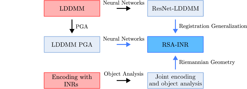
Figure 1: Our novel RSA-INR method can be derived in three different ways. First, RSA-INR extends the ResNet-LDDMM pairwise registration algorithm by adding latent codes. This extension ensures straightforward calculation of correspondences between two new shapes. Alternatively, our model extends shape variability modeling based on LDDMM PGA by adding neural networks. Finally, we consider state-of-the-art INR latent space models for joint shape encoding and shape analysis and add Riemannian geometry to the latent space.

First, we show that our method resembles PGA. More precisely, we establish that the Riemannian regularization is required to simultaneously achieve two objectives: obtaining a template shape as the mean of the data and obtaining physically plausible deformations that align the template to the data. Based on this observation, we also argue that our shape encoding model has an added Riemannian geometry component. In addition, we discuss how our method can easily match two new shapes, thus generalizing ResNet-LDDMM [12]. Finally, we show that the Riemannian geometry leads to better reconstruction generalization compared to the model without it and the model with a regularization that is not based on Riemannian geometry. We also demonstrate that our model is more robust against noise than the other two models. The better reconstructions and the improved stability to noise show that the Riemannian regularizer yields better factors of variation given the shape data. Summarizing, we show how shape/image analysis, Riemannian geometry, and deep learning are connected and can reinforce each other.

The rest of the paper is organized as follows. In Section 2, we put our work into context by discussing related works. Subsequently, we treat the background theory needed for our method. Specifically, we treat the implicit representation of shapes (Section 3.1) and the LDDMM framework (Section 3.2). Section 4 introduces our neural network model that uses a Riemannian regularization, resembles PGA, and allows for groupwise registration. We employ this model in Section 5 where we compare it to the same model without the Riemannian regularization and to the model with a non-Riemannian regularization. Finally, we discuss some limitations of our approach, discuss future work, and summarize the paper in Sections 6 and 7. In the appendices, we provide additional experiments, additional details, and some basics of Riemannian geometry.

2 Related work

In this section, we contextualize our contributions by discussing related literature on principal geodesic analysis (PGA), Riemannian geometry for latent space models, and neural ordinary differential equations (NODE).

2.1 Principal geodesic analysis

Principal component analysis (PCA) is a well-known technique that has applications in, among others, dimensionality reduction, data visualization, and feature extraction. In addition, the probabilistic extension of PCA, called Probabilistic PCA, can also be used to generate new samples from the data distribution [31]. A limitation of PCA and probabilistic PCA is that they can only be applied to Euclidean data and not Riemannian manifold-valued data. To solve this limitation, principal geodesic analysis (PGA) [32] and probabilistic principal geodesic analysis (PPGA) [33] are introduced as extensions of PCA and probabilistic PCA, respectively.

PGA is applied in various domains. For instance, optimal transport (OT) uses PGA to define Fréchet means and interpolations of data distributions called barycenters [34, 35]. Shape analysis uses PGA as well [32]. Different versions of shape PGA are obtained by choosing different Riemannian distances on the shape space. For instance, while in Zhang and Fletcher [36] and Zhang et al. [37] an LDDMM-based distance is used for PGA, Heeren et al. [38] use a thin shell energy as the Riemannian distance. Furthermore, besides shape analysis based on PGA, shape analysis tools exist that use tangent PCA [39, 10] or that use a combination of tangent PCA and geodesic PCA [40].

Similar to how an autoencoder is a nonlinear version of PCA, our encoding framework can be viewed as a nonlinear version of PGA and PPGA. Another neural network model that can be regarded as a nonlinear version of PPGA is the Riemannian variational autoencoder (Riemannian VAE) [41]. The Riemannian VAE only considers learning a latent space for data on finite-dimensional Riemannian manifolds for which the exponential map and the Riemannian distance have an explicit formula. Hence, it is not applicable to the infinite-dimensional Riemannian manifold of shapes for which the LDDMM Riemannian distance does not have an explicit formula. Our deformable template model extends the Riemannian VAE to this setting.

Bone et al. [42] construct a shape VAE that resembles PGA for shapes [36]. Similar to our work, they use an ordinary differential equation (ODE) to deform a learned template shape to a reconstructed shape. Moreover, they introduce a regularizer on the velocity vector fields to let the ODE flow be a diffeomorphism. In contrast, while Bone et al. [42] consider the mesh representation of shapes, we consider the state-of-the-art implicit shape representation. This allows us to get infinite-resolution shape reconstructions because the shapes are represented by the zero level set of a function. In addition, our model extends the regularizer of Bone et al. to allow a rigidity prior on the template deformations. The regularizer enforces a novel Riemannian structure on the implicit encoding space. Finally, in contrast to their work, we are more interested in the effect of the regularization. First, we investigate whether the Riemannian regularization is needed for the model to resemble PGA. Hence, we examine if Riemannian regularization is necessary to jointly learn a proper template shape and physically plausible deformations from the template to the (reconstructed) training data. Moreover, we demonstrate that the Riemannian regularization helps reconstruction generalization and helps the stability of the reconstruction process.

2.2 Riemannian geometry for latent space models

Latent space models based on neural networks are used for, among others, dimensionality reduction, clustering, and data augmentation. Most of these models have the drawback that distances between latent codes do not always correspond to a ’semantic’ distance between the objects they represent. One mathematical tool to solve this issue is Riemannian geometry. Arvanitidis et al. [43] design a Riemannian distance between latent codes by defining the corresponding Riemannian metric. This metric is defined as the standard Euclidean metric pulled back under the action of the decoder. The shortest paths under this Riemannian metric are found by solving the geodesic equation via a numerical solver. However, one can also find the shortest path by solving the geodesic equation via Gaussian processes and fixed point iterations [44]. Another approach is to solve the geodesic minimization problem [45, 46]. In Arvanitidis et al. [47] a surrogate Riemannian metric is proposed that approximates the Euclidean pullback metric and yields more robust calculations of shortest paths. In Chadebec et al. [46], the Riemannian metric is incorporated into a Hamiltonian Markov Chain to sample from the posterior distribution of a VAE. Geng et al. [48] enforce a Riemannian distance structure by encouraging Euclidean distances in latent space to equal the Riemannian distance in the original space. Consequently, linear interpolations correspond to points on the learned manifold.

Besides using the Riemannian metrics and the shortest paths for defining good distances, creating good interpolations, and defining probability distributions on the latent space, they are also used for improved shape generation [46], for improved clustering [49, 46], and for data augmentation [50].

The nonlinear PGA that we deploy is related to the Riemannian geometry for latent space models literature. The reason is that we embed a Riemannian distance between a learned template shape and the other shapes by using LDDMM as Riemannian distance.

2.3 Neural ODEs

The neural ODE (NODE) [51] is a first-order differential equation where the time derivative is parameterized by a neural network. It has applications in learning dynamics [52, 53, 54, 55], control [56, 57], generative modeling [51, 58], and joint shape encoding, reconstruction, and registration [59, 19, 29]. Furthermore, there is a bidirectional connection between the NODE and optimal transport (OT). First, due to the fluid dynamics formulation of OT [60], NODEs can be used to solve high-dimensional OT problems [61]. In addition, the learned dynamics can be complex and require many time steps to be solved accurately. As a consequence, training NODEs can be challenging and time-consuming. OT-inspired regularization functionals solve this issue as they simplify the dynamics and reduce the time needed to solve the NODE [62, 63].

Our framework fits the bidirectional connection of NODEs and OT. First, we use a neural ODE to solve the LDDMM problem, which is a problem that in formulation bears similarities to the fluid dynamics formulation of OT. Hence, our approach shares similarities with the works using NODEs to solve OT problems. In addition, we use cost functionals inspired by LDDMM to regularize the NODE used for shape matching. This fits the works that use OT for regularizing the dynamics of NODEs.

3 Preliminaries

3.1 Implicit shape representations

Recently, the implicit shape representation has emerged in state-of-the-art deep learning algorithms dealing with shapes. A shape $\mathcal{S}:=\{x\mid f(x)=c\}$ is described by the $c$ level set of a function $f:\Omega\rightarrow\mathbb{R}$ on the image domain $\Omega\subset\mathbb{R}^{d}$. Two examples of common implicit representations are the signed distance function (SDF) with $c=0$ and the occupancy function with $c=0.5$, respectively:

$$\text{SDF}_{\mathcal{S}}(x) =\begin{aligned} \begin{cases}\inf_{y\in\mathcal{S}}\lVert x-y\rVert_{2}\quad\quad\text{if }x\text{ outside }\mathcal{S},\\ -\inf_{y\in\mathcal{S}}\lVert x-y\rVert_{2}\quad\text{if }x\text{ inside }\mathcal{S},\\ \end{cases}\end{aligned}$$ (1)

$$\text{OCC}_{\mathcal{S}}(x) =\begin{aligned} \begin{cases}0\qquad\qquad\qquad\qquad\text{if }x\text{ outside }\mathcal{S},\\ 0.5\qquad\qquad\qquad\quad\,\text{if }x\in\mathcal{S},\\ 1\qquad\qquad\qquad\qquad\text{if }x\text{ inside }\mathcal{S}.\\ \end{cases}\end{aligned}$$ (2)

As opposed to the more traditional discrete representations such as point clouds, meshes, or voxel grids, the implicit shape representation is a continuous representation as it represents the shape using a function. As a consequence, we can obtain a mesh or point cloud at an arbitrary resolution by using marching cubes [64]. Unlike the discrete representations, the implicit representation has the disadvantage that it does not provide point correspondences between shape deformations.

3.2 Diffeomorphic shape matching and a distance on shape space

To match two shapes $\mathcal{S}$ and $\mathcal{T}$, a function $f(x)$ is constructed that assigns to each point $x\in\mathcal{S}$ a point $f(x)\in\mathcal{T}$ in a meaningful way. For instance, when comparing two human shapes, one wants to match points on the arm of one human with points on the same arm of the other human.

In this work, we focus on the diffeomorphic registration framework called Large Deformation Diffeomorphic Metric Mapping (LDDMM) [6]. The objective of LDDMM is to find a diffeomorphism $\phi:\Omega\rightarrow\Omega$ that matches two objects $O_{1}$ and $O_{2}$ (e.g., images or shapes defined on $\Omega\subset\mathbb{R}^{d}$) by deforming $O_{1}$ into $O_{2}$. More precisely, LDDMM wants $\phi\cdot O_{1}=O_{2}$ with $\phi\cdot O$ a left group action of the diffeomorphism group on the set of objects. For instance, an image $I:\Omega\rightarrow\mathbb{R}^{n}$ can be deformed by a left group action $\phi\cdot I:=I\circ\phi^{-1}$ and a shape $\mathcal{S}:=\{x\mid x\text{ on the shape}\}$ can be deformed by a left group action $\phi\cdot\mathcal{S}:=\phi(\mathcal{S})$.

To construct a diffeomorphism that achieves $\phi\cdot O_{1}=O_{2}$, LDDMM considers a subgroup of the diffeomorphism group. This subgroup consists of diffeomorphisms emerging as flows of ordinary differential equations (ODEs). Define a time dependent vector field $v:\Omega\times[0,1]\rightarrow\mathbb{R}^{d}$ and assume $v_{t}:=v(\cdot,t)\in V$ for some Hilbert space $V$. The corresponding ODE is $\frac{\mathrm{d}x}{\mathrm{d}t}=v_{t}(x)$ and it gives us a flow of diffeomorphisms:

$$\frac{\partial\phi}{\partial t}(x,t) =v_{t}(\phi(x,t)),$$ (3)

$$\phi(x,0) =x.$$

To make these ODE flows diffeomorphisms, one has to enforce smoothness on the velocity vector fields $v_{t}\in V$. Generally, this is accomplished by choosing an appropriate normed space $V$ and assuming $v\in L^{1}([0,1],V)$ [6, 10, 65]. For conciseness, we leave out the details.

Using these considerations, the subgroup that LDDMM considers is defined as

$$G:=\{\phi_{1}\mid\phi_{1}(\cdot):=\phi(\cdot,1)\text{ for }\phi\text{ in Equation \eqref{eq:ode_diffeo}},v\in L^{1}([0,1],V)\}.$$ (4)

There might exist multiple $\phi\in G$ such that $\phi\cdot O_{1}=O_{2}$ for objects $O_{1}$ and $O_{2}$. The LDDMM approach selects the ’smallest’ $\phi\in G$ such that $\phi\cdot O_{1}=O_{2}$. To define ’smallest’, LDDMM uses the following Riemannian distance $\rho_{G}$ on $G$:

$$\rho_{G}(\phi_{0},\phi_{1}):=\inf_{\phi\in G}\left(\int_{0}^{1}\lVert v_{t}\rVert_{V}\mathrm{d}t\mid\phi_{1}=\phi\circ\phi_{0}\right),$$ (5)

where $\lVert\cdot\rVert_{V}$ is a norm on $V$. The LDDMM approach selects the $\phi\in G$ such that $\phi\cdot O_{1}=O_{2}$ and $\rho_{G}(\text{id},\phi)$ is small. Alternatively, we can reformulate this problem as finding a distance between two objects $O_{1}$ and $O_{2}$:

Theorem 1 ([6]).

Assume $\lVert\cdot\rVert_{V}$ is a norm on $V$ and $\rho_{G}$ is given by equation (5). Then we can define a distance $\rho_{\mathcal{O}}(O_{1},O_{2})$ as

$$\rho_{\mathcal{O}}(O_{1},O_{2}):=\inf_{\phi\in G}\left(\rho_{G}({\text{id}},\phi)\mid O_{2}=\phi\cdot O_{1}\right)$$ (6)

or alternatively:

$$\rho_{\mathcal{O}}(O_{1},O_{2})=\min_{v_{t}} \left(\int_{0}^{1}\lVert v_{t}\rVert_{V}\mathrm{d}t\right)$$ (7)

s.t. $$\frac{\mathrm{d}\phi_{t}}{\mathrm{d}t}=v_{t}(\phi_{t}),\quad\phi_{0}={\text{id}},$$

$$\phi_{1}\cdot O_{1}=O_{2}.$$

As mentioned above, the goal of LDDMM is to approximately solve Equations (6) and (7). However, it is known that the solution $\phi_{t}$ to Equation (7) is reparameterization invariant. Hence, there exists an infinite number of $\phi_{t}$ that trace out the same curve in the diffeomorphism group and that all have the same integral cost. To resolve this issue, LDDMM minimizes an energy that is not reparameterization invariant. This is possible by the following theorem:

Theorem 2 ([6]).

Assume $\lVert\cdot\rVert_{V}$ is a norm on $V$. Then we can define the energy $E_{G}$ between two diffeomorphisms as

$$E_{G}(\phi_{0},\phi_{1}):=\inf_{\phi\in G}\left(\int_{0}^{1}\lVert v_{t}\rVert_{V}^{2}\mathrm{d}t\mid\phi_{1}=\phi\circ\phi_{0}\right).$$

Moreover, we define the induced energy $E_{\mathcal{O}}$ as

$$E_{\mathcal{O}}(O_{1},O_{2}):=\inf_{\phi\in G}\left(E_{G}({\text{id}},\phi)\mid O_{2}=\phi\cdot O_{1}\right)$$

or alternatively:

$$E_{\mathcal{O}}(O_{1},O_{2})=\min_{v_{t}} \left(\int_{0}^{1}\lVert v_{t}\rVert_{V}^{2}\mathrm{d}t\right)$$ (8)

s.t. $$\frac{\mathrm{d}\phi_{t}}{\mathrm{d}t}=v_{t}(\phi_{t}),\quad\phi_{0}={\text{id}},$$

$$\phi_{1}\cdot O_{1}=O_{2}.$$

It can be shown that any $\phi_{t}$ solving the energy minimization problem (8) solves the distance problem in Equation (7). Conversely, any constant speed curve $\phi_{t}\in G$ (i.e., $\lVert v_{t}\rVert_{V}$ stays constant over time) that solves the distance problem in Equation (7) solves the energy minimization problem in Equation (8).

Using Theorem 2, LDDMM solves optimization problem (8) instead of optimization problem (7). To solve the energy minimization problem (8), LDDMM solves the relaxed problem:

$$\min_{v_{t}} \left(\int_{0}^{1}\lVert v_{t}\rVert_{V}^{2}\mathrm{d}t\right)+\frac{1}{\sigma^{2}}\mathcal{D}(\phi_{1}\cdot O_{1},O_{2})$$ (9)

s.t. $$\frac{\mathrm{d}\phi_{t}}{\mathrm{d}t}=v_{t}(\phi_{t}),\quad\phi_{0}=\text{id},$$

where $\mathcal{D}$ is some data fidelity term and $\sigma\in\mathbb{R}$. For instance, when dealing with images, one can use $\mathcal{D}(I_{1},I_{2})=\lVert I_{1}-I_{2}\rVert_{L_{2}(\Omega)}^{2}$ and $\phi\cdot I=I\circ\phi^{-1}$.

4 Riemannian autodecoder for implicit shape representation

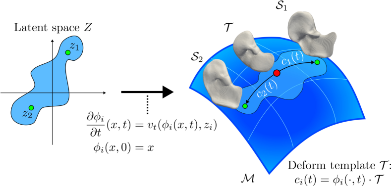
Figure 2: Overview of our framework. We map a latent vector $z_{i}$ to a time dependent velocity vector field $v_{t}(\cdot,z_{i}):=v(\cdot,t,z_{i})$. This defines a flow of diffeomorphisms $\phi_{i}$ via an ODE. The diffeomorphism $\phi_{i}(\cdot,1)$ creates (reconstructed) shapes $\mathcal{S}_{i}$ on a nonlinear non-geodesic subset of the Riemannian shape manifold $\mathcal{M}$ by deforming a learned template $\mathcal{T}$ via a group action: $c_{i}(t)=\phi_{i}(\cdot,t)\cdot\mathcal{T}$. The goal is to learn the template $\mathcal{T}$ as Fréchet mean of the data and to learn the $c_{i}(t)$ paths as geodesics on $\mathcal{M}$ between the template $\mathcal{T}$ and the data.

In this section, we introduce our novel implicit shape encoder. First, we explain how our deformable template model (see Figure 2) and our loss function are derived from the Fréchet mean finding problem in LDDMM PGA. Subsequently, we parameterize the template by an INR, choose the data fitting term, and choose the regularization terms. Finally, we treat how we numerically deform the template to obtain a reconstruction of a shape and we treat how we can obtain latent codes for unseen shapes.

4.1 Autodecoder based on principal geodesic analysis

Our model builds upon the LDDMM method, which was discussed in Section 3.2. Moreover, it extends the model proposed by Sun et al. [29] by adding an LDDMM-inspired regularization term. We now treat how our model can be derived from the LDDMM Fréchet mean problem [13, 66, 14, 15], in particular from PGA that uses an LDDMM distance [36, 37].

Assume we want to find the Fréchet mean based on LDDMM PGA [36, 37]. The Fréchet mean $\mathcal{T}$ should solve:

$$\min_{\mathcal{T}} \operatorname*{\mathop{\mathbb{E}}}_{\mathcal{S}\sim\rho(S)}\left[\rho_{\mathcal{O}}(\mathcal{T},\mathcal{S})^{2}\right],$$

with $\rho(\mathcal{S})$ the distribution of shapes and $\rho_{\mathcal{O}}$ given as the distance in Equations (6) and (7). Using Theorem 2 and the fact that we can normalize any curve $\phi_{t}$ to have constant $\lVert v_{t}\rVert_{V}$, we can also minimize:

$$\min_{\mathcal{T}} \operatorname*{\mathop{\mathbb{E}}}_{\mathcal{S}\sim\rho(S)}\left[E_{\mathcal{O}}(\mathcal{T},\mathcal{S})\right].$$

Writing out $E_{\mathcal{O}}$ using Equation (8) and approximating the expectation using $N$ training samples, we get:

$$\min_{\{v_{i}(\cdot,t)\}_{i=1}^{N},\mathcal{T}} \frac{1}{N}\sum_{i=1}^{N}\left[\int_{0}^{1}\lVert v_{i}(\cdot,t)\rVert_{V}^{2}\mathrm{d}t\right]$$ (10)

s.t. $$\frac{\mathrm{d}\phi_{i}}{\mathrm{d}t}(x,t)=v_{i}(\phi_{i}(x,t),t),\quad\phi_{0}=\text{id},$$

$$\phi_{i}(\cdot,1)\cdot\mathcal{T}=\mathcal{S}_{i}.$$

As in LDDMM, we turn the hard constraint into a soft constraint using a data fitting term $\mathcal{D}$ and a $\sigma\in\mathbb{R}$:

$$\min_{\{v_{i}(\cdot,t)\}_{i=1}^{N},\mathcal{T}} \frac{1}{N}\sum_{i=1}^{N}\left[\mathcal{D}\left(\phi_{i}(\cdot,1)\cdot\mathcal{T},\mathcal{S}_{i}\right)+\sigma^{2}\int_{0}^{1}\lVert v_{i}(\cdot,t)\rVert_{V}^{2}\mathrm{d}t\right]$$

s.t. $$\frac{\mathrm{d}\phi_{i}}{\mathrm{d}t}(x,t)=v_{i}(\phi_{i}(x,t),t),\quad\phi_{0}=\text{id}.$$

Finally, we parameterize the unknowns. We parameterize $\phi_{i}(\cdot,1)$ by specifying the corresponding flow in reverse time. Defining $z_{i}$ as the latent code belonging to the shape $\mathcal{S}_{i}$ and defining $v_{\varphi}$ as a neural network, the reverse time flow is given by $\frac{\mathrm{d}\phi_{t}}{\mathrm{d}t}(x,z_{i})=v_{\varphi}(\phi_{t}(x,z_{i}),t,z_{i})$. Moreover, we represent the template by $\mathcal{T}_{\theta}$ for some parameters $\theta$. Combining this with an autodecoder strategy [24, 29] yields the final loss function:

$$\min_{\theta,\varphi,\{z_{i}\}_{i=1}^{N}} \frac{1}{N}\sum_{i=1}^{N}\left[\mathcal{D}(\phi_{1}(\cdot,z_{i})^{-1}\cdot\mathcal{T}_{\theta},\mathcal{S}_{i})+\sigma^{2}\int_{0}^{1}\lVert v_{\varphi}(\cdot,t,z_{i})\rVert_{V}^{2}\mathrm{d}t\right]$$ (11)

s.t. $$\frac{\mathrm{d}}{\mathrm{d}t}\phi_{t}(x,z_{i})=v_{\varphi}(\phi_{t}(x,z_{i}),t,z_{i}),\quad\phi_{0}=\text{id}.$$

Hence, we do not use an encoder. We only need to optimize the decoder $\phi_{1}(\cdot,\cdot)^{-1}\cdot\mathcal{T}_{\theta}$ and the latent codes $z_{i}$ to reconstruct the training data. In Section 4.5, we discuss how to obtain latent codes of unseen shapes using the autodecoder. For more information on autodecoders, we refer to the work of Park et al. [24].

After training, we can decode and reconstruct shapes by deforming $\mathcal{T}_{\theta}$ via the group action $\phi_{1}(\cdot,z)^{-1}\cdot\mathcal{T}_{\theta}$. This also ensures that the reconstruction is matched to the template. Consequently, we can match unseen shapes with each other by pairing points that map to the same point on $\mathcal{T}_{\theta}$. Hence, we perform a groupwise registration using neural networks and generalize ResNet-LDDMM [12].

Remark 1.

Our derivation shows that the learned template shape $\mathcal{T}_{\theta}$ should represent a Fréchet mean of the data. To compute the Fréchet mean, we calculate the energies $E_{\mathcal{O}}(\mathcal{T}_{\theta},\mathcal{S}_{i})$ via the $v_{i}$ in Equation (10) and the $v_{\varphi}$ in Equation (11). Hence, according to Theorem 2, we can use the decoder to estimate the distances $\rho_{\mathcal{O}}(\mathcal{T}_{\theta},\mathcal{S})$ for reconstructed shapes $\mathcal{S}$. Furthermore, by definition of $\rho_{\mathcal{O}}$, the deformation $\phi_{t}(\cdot,z_{i})\cdot\mathcal{S}_{i}$ should represent a geodesic from $\mathcal{S}_{i}$ to the learned template $\mathcal{T}_{\theta}$. Hence, if trained perfectly, the decoder transforms the template shape via a shape space geodesic to the reconstructed shapes. Overall, we are enforcing a Riemannian structure on the latent space.

4.2 Choice of data fidelity

In this work, we represent the learnable template shape $\mathcal{T}_{\theta}$ via an implicit representation (see Section 3.1). We make the template shape learnable by parameterizing the implicit function representation by a neural network $f_{\theta}:\mathbb{R}^{3}\rightarrow\mathbb{R}$, making $f_{\theta}$ an implicit neural representation (INR) [24, 26, 25, 67]. In this case, we define the group action in Equation (11) by

$$I(x,z,t)=((\phi_{t}(\cdot,z))^{-1}\cdot f_{\theta})(x):=f_{\theta}(\phi_{t}(x,z)),$$ (12)

where $I(x,z,0)$ equals the implicit representation of the template shape and $I(x,z,1)$ is the reconstructed implicit representation of a shape $\mathcal{S}$. We can get a mesh and point cloud for the reconstructed shape by applying marching cubes on $I(x,z,1)$. Another strategy is to apply marching cubes to the template INR $f_{\theta}$ to get a template mesh $\mathcal{M}_{\mathcal{T}}$ and then get the reconstructed mesh $\mathcal{M}_{z}$ by $\phi_{1}^{-1}(\mathcal{M}_{\mathcal{T}},z)$.

To fit the reconstructed implicit functions $I(x,z_{i},1)$ to the shapes $\mathcal{S}_{i}$, we need to choose a proper $\mathcal{D}$ in Equation (11). Recent works that employ a deformable template for joint shape encoding and registration [28, 29] use $\mathcal{D}(I_{1},I_{2})=\lVert I_{1}-I_{2}\rVert_{L_{2}(\Omega)}^{2}$ with $I_{i}$ an implicit representation of a shape. However, there are two issues with this data fitting term.

First, assume we have two circles of radii $0.75$ and $0.1$, respectively. Moreover, assume they are represented by their SDF, as presented in Equation (1). These SDFs are shown in Figure 3.

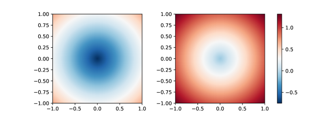
Figure 3: SDF values in $[-1,1]^{2}$ of a circle with radius $0.75$ (left) and of a circle with radius $0.1$ (right).

We note that $\min_{x\in\Omega}\text{SDF}_{\mathcal{S}_{0}}(x)<\min_{x\in\Omega}\text{SDF}_{\mathcal{S}_{1}}(x)$ as dark blue is present in the figure of the circle with radius $0.75$ but not in the other figure. This means there does not exist a diffeomorphism that matches the two implicit representations (i.e., SDF images). However, in Equation (11) we want to diffeomorphically match both to the same template implicit function. This is not possible as the two SDFs can not be diffeomorphically matched.

Additionally, a specific choice of implicit function influences the diffeomorphism we find. Assume shapes $\mathcal{S}_{0}$ and $\mathcal{S}_{1}$ are represented by implicit functions that can be exactly matched. If a point $x_{0}$ in shape $\mathcal{S}_{0}$ has implicit function value $s$, it must be matched with a point $x_{1}$ in shape $\mathcal{S}_{1}$ that also has implicit function value $s$. By also matching points outside and inside the shape based on information like the SDF value, we influence how the points on the shape are matched.

To overcome these issues, we take inspiration from an approach that learns signed distance functions for meshes and point clouds [67]. Our approach uses the point cloud representation for the training shapes $\{\mathcal{S}_{i}\}_{i=1}^{N}$ and uses the following data fidelity term $\mathcal{D}$:

$$\mathcal{D}(\phi_{1}(\cdot,z)^{-1}\cdot\mathcal{T}_{\theta},\mathcal{S}_{i})=\operatorname*{\mathop{\mathbb{E}}}_{x\in\mathcal{S}_{i}}\left[\lvert I(x,z,1)\rvert+\tau\left(1-F_{\text{cos}}(\nabla_{x}I(x,z,1),n_{i}(x))\right)\right],$$

with $\tau\in\mathbb{R}$, $n_{i}(x)$ the unit normal of the shape $\mathcal{S}_{i}$ at $x\in\mathcal{S}_{i}$, and $F_{\text{cos}}$ the cosine similarity:

$$F_{\text{cos}}(a,b)=\frac{\langle a,b\rangle_{2}}{\max(\lVert a\rVert_{2},\lVert b\rVert_{2},10^{-8})}.$$

This data fitting term solves the previously mentioned issues since it only focuses on matching points on the training shapes with points on the template shape. In other words, all points on the training shapes are matched to the zero level set of the INR $f_{\theta}$. However, using only this loss function encourages $f_{\theta}=0$ as this ensures that all points are matched to the zero level set of $f_{\theta}$. To avoid this trivial template shape, we constrain the learned template in optimization problem (11) via additional loss terms:

$$\min_{\theta,\varphi,\{z_{i}\}_{i=1}^{N}} \frac{1}{N}\sum_{i=1}^{N}\left[\operatorname*{\mathop{\mathbb{E}}}_{x\in\mathcal{S}_{i}}\left[\lvert I(x,z_{i},1)\rvert+\tau\left(1-F_{\text{cos}}(\nabla_{x}I(x,z_{i},1),n_{i}(x))\right)\right]\right.$$ (13)

$$\left.\qquad\quad+\beta\operatorname*{\mathop{\mathbb{E}}}_{x\in\Omega\setminus\mathcal{S}_{i}}\left[\exp{(-\alpha\lvert I(x,z_{i},1)\rvert)}\right]+\sigma^{2}\int_{0}^{1}\lVert v_{\varphi}(\cdot,t,z_{i})\rVert_{V}^{2}\mathrm{d}t\right]$$

$$+\lambda\operatorname*{\mathop{\mathbb{E}}}_{x\in\Omega}\left[\lvert\lVert\nabla_{x}f_{\theta}(x)\rVert_{2}-1\rvert\right]$$

s.t. $$\frac{\mathrm{d}}{\mathrm{d}t}\phi_{t}(x,z_{i})=v_{\varphi}(\phi_{t}(x,z_{i}),t,z_{i}),\quad\phi_{0}=\text{id},$$

$$I(x,z,t):=((\phi_{t}(\cdot,z))^{-1}\cdot f_{\theta})(x):=f_{\theta}(\phi_{t}(x,z)).$$

Here the penalty corresponding to $\lambda\in\mathbb{R}$ is an eikonal penalty, regularizing the template shape to be a signed distance function as in Equation (1). This ensures that $f_{\theta}\neq 0$. Furthermore, the loss function involving the $\beta$ parameter ensures that only points on $\mathcal{S}_{i}$ are matched to the zero level set of $f_{\theta}$. Both terms are inspired by Sitzmann et al. [25], Deng et al. [27], and Gropp et al. [67].

Remark 2.

Another approach to solve the issues is using the occupancy function in Equation (2) as an implicit representation for the data and for the template shape. Earlier works using occupancy functions as implicit representations are Mescheder et al. [26] and Niemeyer et al. [59]. The reason occupancy functions solve the issues is that we only match points inside (outside) shape $\mathcal{S}_{0}$ to points inside (outside) shape $\mathcal{S}_{1}$ and do not take into account information like the SDF value. As the occupancy function and the occupancy values resemble probabilities, we would use the binary cross entropy loss as data fidelity term $\mathcal{D}$ in optimization problem (11) [26, 59]. However, as shown in Appendix C, our strategy that uses point clouds as data representation allows for higher-quality reconstructions. As a consequence, we use the point cloud data representation instead of the occupancy value data representation.

4.3 Choice of velocity field regularization term

For the norm $\lVert\cdot\rVert_{V}$ in optimization problem (11) we choose an isometric (rigid) deformation prior on the velocity vector fields by combining the Killing energy [68, 69] with an $L_{2}(\Omega)$ penalty:

$$\lVert v\rVert_{V}^{2}:=\int_{\Omega}\lVert(J_{x}v)+(J_{x}v)^{T}\rVert_{F}^{2}+\eta\lVert v\rVert^{2}_{2}\mathrm{d}x,$$ (14)

where $J_{x}v$ is the Jacobian of $v$ with respect to $x$ and $\eta\in\mathbb{R}$. If $\eta$ and the functional in Equation (14) are small, then we expect the template shape to deform almost isometrically to the reconstructed shapes via $I(x,z,t)$ in Equation (12). Moreover, as shown in Appendix B, under certain conditions the Killing energy can be viewed as an extension of a standard norm used in LDDMM.

4.4 Solving the ordinary differential equation

To solve optimization problems (11) and (13), we need to parameterize the velocity vector field $v_{\varphi}$ and solve the resulting ordinary differential equation. Similarly to Gupta et al. [19] and Sun et al. [29], our model parameterizes $v_{\varphi}$ as a quasi-time-varying velocity vector field. Concretely, using $\chi_{A}$ as the indicator function of $A$, we define $K$ neural networks $v_{\varphi_{k}}:\Omega\rightarrow\mathbb{R}^{d}$ representing stationary velocity fields and define $v_{\varphi}$ as

$$v_{\varphi}(x,t)=\sum_{k=1}^{K}\chi_{[\frac{k-1}{K},\frac{k}{K}]}(t)\cdot v_{\varphi_{k}}(x).$$ (15)

The main reason for this parameterization is that training time-varying velocity vector fields can be difficult as the model does not have training data for $0<t<1$. During training, we solve the ODE using an Euler discretization with $K$ time steps. Consequently, similar to ResNet-LDDMM [12], we approximate the ODE with a ResNet architecture.

4.5 Encoding objects

We use the strategy from DeepSDF [24] to encode (new) objects. More precisely, we solve the following optimization problem for encoding the object $\mathcal{S}$:

$$\min_{z}\mathcal{D}_{rec}(\phi_{1}(\cdot,z)^{-1}\cdot\mathcal{T}_{\theta},\mathcal{S})+\gamma\lVert z\rVert_{2}^{2},$$ (16)

where $\gamma\in\mathbb{R}$, $\phi_{1}$ is defined via the ODE in optimization problems (11) and (13), $\mathcal{T}_{\theta}$ is the learned template, and $\mathcal{D}_{rec}$ is some reconstruction data fitting term. For instance, in case $\mathcal{S}$ is represented by a mesh or a point cloud, we use $\operatorname*{\mathop{\mathbb{E}}}_{x\in\mathcal{S}}\left[\lvert I(x,z,1)\rvert\right]$ as $\mathcal{D}_{rec}$ with $I(x,z,t)$ given by Equation (12).

Remark 3.

Our encoding procedure presented in Equation (16) can be viewed as a nonlinear extension of the encoding strategy in PGA [32]. In PGA, the first step is to find the Fréchet mean $\mu$ of the data. Subsequently, PGA identifies a subspace $V$ of the tangent space $T_{\mu}M$ such that most variability in the data is described by $H=\text{Exp}_{\mu}(V)$, where $\text{Exp}_{\mu}$ is the exponential map at $\mu$. Finally, to project a data point $x\in M$ onto $H$, one calculates:

$$\pi_{H}(x)=\arg\min_{y\in H}d(x,y)^{2},$$

where $d$ is the Riemannian distance on the Riemannian manifold $M$. Alternatively, this can be reformulated into a minimization over the subspace $V$:

$$\arg\min_{v\in V}d(x,\text{Exp}_{\mu}(v))^{2}.$$

Equation (16) resembles this optimization problem. First, we have $x=\mathcal{S}$. Furthermore, $\phi_{1}(\cdot,z)^{-1}\cdot\mathcal{T}_{\theta}$ should approximate $\text{Exp}_{\mu}$ in case we consider the LDDMM manifold with $\mu=\mathcal{T}_{\theta}$. Although $\mathcal{D}_{rec}$ is not a Riemannian distance, it replaces the Riemannian distance $d$, as also done in, e.g., Charlier et al. [40]. Finally, instead of searching over the vector space $V$, we search over a latent space that defines $\phi_{1}(\cdot,z)^{-1}\cdot\mathcal{T}_{\theta}$. Hence, instead of finding an initial velocity $v\in V$ to define a point $y=\text{Exp}_{\mu}(v)$ on the manifold, we find a latent code $z$ that determines a point on the manifold.

5 Numerical results

We compare our model that uses the Riemannian integral regularization on the flow (see Equation (13)) to our model without flow regularization and to our model using the pointwise regularization as presented in Appendix D.2. The latter model is the baseline model by Sun et al. [29] with a different data fitting term and a different approach to solving the ordinary differential equation. First, we show that only our Riemannian model can be seen as a nonlinear PGA. We achieve this by visualizing the learned templates and the learned deformations from the template to the training shapes, and we argue that only the model with the integral regularization incorporates a Riemannian geometry aspect in the latent space. Subsequently, we discuss reconstruction generalization and robustness of the reconstruction procedure to noisy data. This discussion shows the effect of our Riemannian regularizer on the quality and stability of the reconstruction procedure.

We conducted these experiments on two datasets: a synthetic rectangles dataset and a shape liver dataset [29, 70]. For details about the data source, the data preprocessing, and the training, we refer to Appendix D.

5.1 Learning shape fréchet means

After training, we obtain the template shapes in Figures 4 and 5. We notice that regularization is necessary to get a template shape that represents the mean of the data. When using regularization, the templates look almost identical for the liver dataset. On the other hand, the templates for the rectangles dataset differ. The difference stems from the used $\eta$ parameter in Equation (14), where $\eta=0.05$ for the rectangles dataset and $\eta=50$ for the liver dataset. We choose $\eta=0.05$ for the rectangles dataset as we expect rigid body motions from the template to the training shapes. For the liver dataset, we do not expect such rigid body motions and pick $\eta$ larger.

As $\eta=50$ for the liver dataset, $\lVert\cdot\rVert_{V}\approx\eta\lVert\cdot\rVert_{L_{2}(\Omega)}$. The pointwise loss can be interpreted as a non-Riemannian version of the integral regularization with $\lVert\cdot\rVert_{V}=\lVert\cdot\rVert_{L_{2}(\Omega)}$ (see Appendix D.2). Hence, as $\lVert\cdot\rVert_{V}\approx\eta\lVert\cdot\rVert_{L_{2}(\Omega)}$, we expect similar templates in Figure 5. Contrarily, for the rectangles dataset, the Killing energy plays a more prominent role in $\lVert\cdot\rVert_{V}$. As a consequence, we expect almost rigid deformations from the template to the training shape. This results in the square template in Figure 4. As the pointwise loss does not induce an isometry prior and is a non-Riemannian version of the integral regularization with $\lVert\cdot\rVert_{V}=\lVert\cdot\rVert_{L_{2}(\Omega)}$, we get a spherical template. In summary, the integral regularization allows more flexibility in learning a template shape that resembles the data.

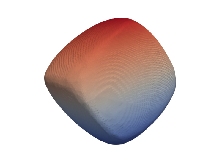
(a) Model using integral regularization.

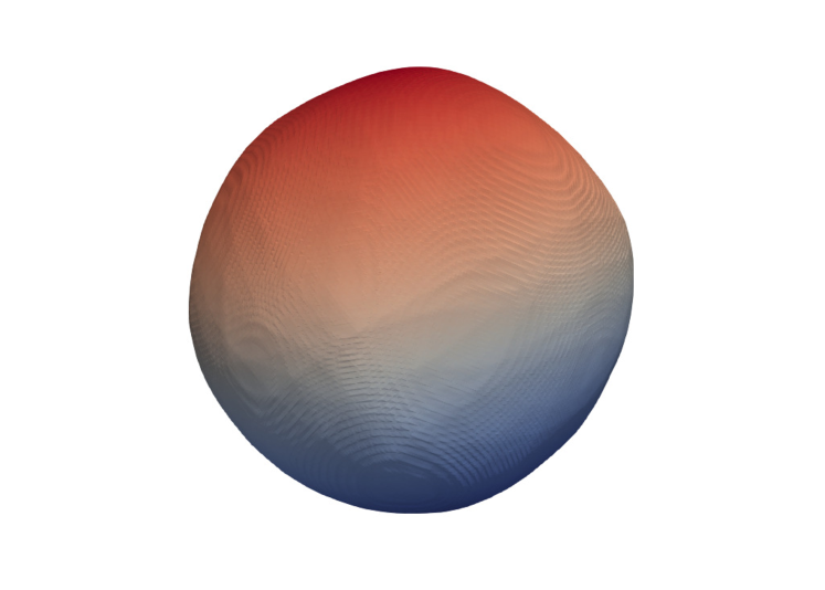
(b) Model using pointwise loss.

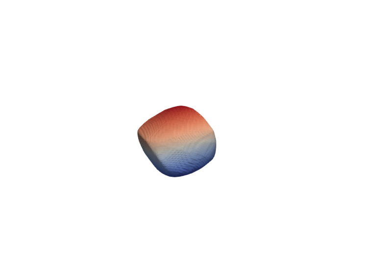
(c) Model using no regularization.

Figure 4: The learned template of three different models trained on the rectangles dataset. We use the model learned using the Riemannian integral regularization (left), the model learned using the pointwise loss (middle), and the model learned using no regularization on the deformation (right). We use $\eta=0.05$ in Equation (14).

(a) Model using integral regularization.

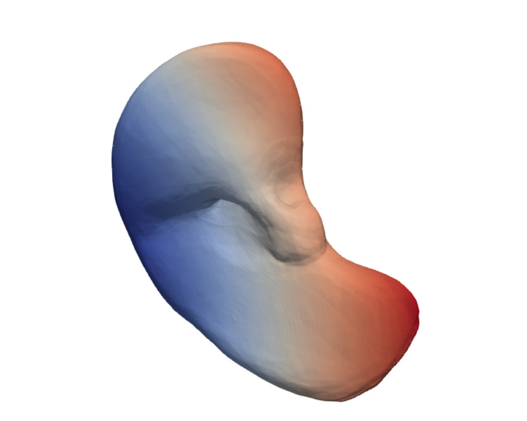
(b) Model using pointwise loss.

(c) Model using no regularization.

Figure 5: The learned template of three different models trained on the liver dataset. We use the model learned using the Riemannian integral regularization (left), the model learned using the pointwise loss (middle), and the model learned using no regularization on the deformation (right). We use $\eta=50$ in Equation (14).

5.2 Joint reconstruction and 4D registration

Figure 6: The deformation of the template into a reconstructed rectangle using the model learned using the Riemannian integral regularization (top), using the model learned using the pointwise loss (middle), and using the model learned using no regularization (bottom). The colors represent the matching of the points to their template.

Figure 7: The deformation of the template into a reconstructed liver using the model learned using the Riemannian integral regularization (top), using the model learned using the pointwise loss (middle), and using the model learned using no regularization (bottom). The colors represent the matching of the points to their template.

In Figure 6 the template is transformed into a reconstructed training shape for each model trained on the rectangles dataset. We notice that the model without regularization does not provide a smooth deformation. Furthermore, the pointwise loss model first enlarges the spherical template and at the end compresses the shape to the reconstructed shape. In contrast, the model with the Riemannian integral regularization smoothly rotates and scales the rectangular template shape to the final reconstructed shape. Hence, it fits the rigid body motion prior induced by the Killing energy. As the pointwise loss does not penalize non-smooth deformations and does not use a rigid body motion prior, we get non-smooth and non-rigid deformations in this case.

In Figure 7 we once more notice that the model without regularization does not ensure smooth deformations of the template shape. Moreover, we notice that the deformation using the Riemannian integral regularization is much smoother than with the pointwise loss. The utilization of the pointwise loss results in physically implausible deformations because it encourages a rapid transition to the target shape followed by a tendency to stay in a nearly identical configuration. In contrast, with the integral regularization, such rapid transitions are penalized, and it is preferred to gradually get closer to the target shape. As a consequence, the integral regularization allows for a smooth, physically plausible template deformation into the reconstructed shapes.

In summary, we need to regularize the deformation to get a decent template shape. The integral regularization is more flexible in influencing the template than the pointwise loss. Moreover, the integral regularization is needed to obtain geodesic deformations of the template to the reconstructions. Hence, only the model with the Riemannian integral regularization is a nonlinear PGA. This model allows us to calculate Fréchet means of the data, to calculate physically plausible geodesic deformations between the template shape and another shape, and to approximate the Riemannian distance between the template and a target shape. Hence, we have added Riemannian geometry to the latent space model.

5.3 Generalizability of shape encoding

This section evaluates the reconstruction quality of the three different models by reconstructing the test sets of the rectangles and liver dataset. We use the Chamfer Distance (CD) and the Earth Mover Distance (EM) as evaluation metrics. Table 1 shows the reconstruction metrics of the training data. We see that all models perform approximately equally on the training data.

Table 1: Average value and standard deviation (between brackets) of the Chamfer Distance (CD) and Earth Mover distance (EM). The values are obtained by reconstructing the training sets of the rectangles (Rect.) and liver dataset. The Chamfer Distance values and standard deviations are of the order $10^{-4}$.

Model	Dataset (metric)
	Rect. (CD)		Rect. (EM)		Liver (CD)		Liver (EM)
No reg.	$0.26$	$(0.078)$	$0.0183$	$(0.0041)$	$0.991$	$(0.422)$	$0.0271$	$(0.0029)$
PW	$0.24$	$(0.085)$	$0.0179$	$(0.0042)$	$1.12$	$(0.515)$	$0.0273$	$(0.0031)$
Riem. reg.	$0.33$	$(0.095)$	$0.0188$	$(0.0044)$	$1.12$	$(0.491)$	$0.0273$	$(0.0035)$

Table 2 shows the reconstruction metrics on the test sets. We can immediately see that the model with Riemannian integral regularization performs the best in terms of average Chamfer Distance. In terms of Earth Mover distance, it is the best on the rectangles dataset and comparable to the model without regularization on the liver dataset. In addition, we see that the model without regularization performs poorly on the rectangles dataset. This is also illustrated in Figure 8 which shows the same reconstructed test shape for each of the models.

Table 2: Average value and standard deviation (between brackets) of the Chamfer Distance (CD) and Earth Mover distance (EM). The values are obtained by reconstructing the test sets of the rectangles (Rect.) and liver dataset. The Chamfer Distance values and standard deviations are of the order $10^{-4}$.

Model	Dataset (metric)
	Rect. (CD)		Rect. (EM)		Liver (CD)		Liver (EM)
No reg.	$84.03$	$(144.61)$	$0.0702$	$(0.0709)$	$6.46$	$(9.52)$	$0.0380$	$(0.0143)$
PW	$5.54$	$(7.15)$	$0.0313$	$(0.0100)$	$13.13$	$(33.21)$	$0.0430$	$(0.0262)$
Riem. reg.	$1.83$	$(1.14)$	$0.0245$	$(0.0056)$	$5.31$	$(5.22)$	$0.0385$	$(0.0128)$

(a) Model using integral regularization.

(b) Model using pointwise loss.

(c) Model using no regularization.

Figure 8: The reconstruction of a rectangle test shape using the model learned using the Riemannian integral regularization (left), using the model learned using the pointwise loss (middle), and using the model learned using no regularization (right). The colors represent the matching of the points with their template (see Figure 6).

A plausible reason for these observations is our rough Euler discretization of the ODE in Equation (13). As discussed in Section 4.4, the Euler discretization during training results in a ResNet architecture similar to the idea in Amor et al. [12]. If the velocity vector field is not regularized, this discretization is not close to the true solution of the ODE and may not be a diffeomorphism. For instance, large displacements and non-smooth deformations can destroy the ODE and diffeomorphism properties. This could explain why the model without regularization fails to generalize on the rectangles dataset (see Figure 8). Furthermore, the pointwise loss allows large displacements, which can cause instabilities in the reconstruction process and might yield worse reconstructions. Disallowing such displacements by applying the Riemannian regularization to the velocity vector fields resolves this problem.

5.4 Robustness to noise

In this section, we investigate how noise affects the reconstruction performance of each of the three models. We add random Gaussian noise with mean zero and standard deviation $0.01$ to the vertices of the meshes in the test set. Subsequently, we reconstruct these noisy meshes and compare them to the noiseless ground truth meshes. The reconstruction of a noisy mesh of the rectangles dataset and of the liver dataset is given in Figure 9. The model with Riemannian integral regularization reconstructs these meshes. The deformation is smooth and the reconstructed shape is noiseless.

Table 3 contains the average reconstruction errors between the reconstructed shapes and the ground truth noiseless shapes. We notice that the model with Riemannian integral regularization is affected the least by the noise. The average values and standard deviations are relatively close to the values in Table 2. Compared to the noiseless case, the models without regularization and with pointwise regularization have very different average reconstruction metrics or very different standard deviations. In particular, for the liver dataset, the pointwise loss model has better reconstruction values when using the noisy data. This shows the instability in the model as noise is needed to stabilize the reconstruction. Hence, we see that using no regularization or using the pointwise regularization yields unstable reconstructions. On the other hand, the Riemannian integral regularization stabilizes the problem and has stable reconstructions.

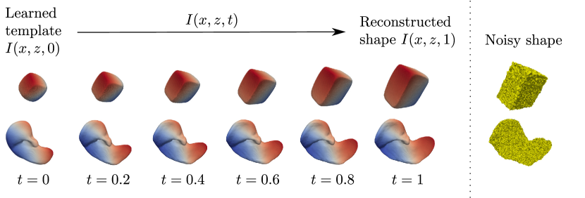
Figure 9: The reconstruction process of two noisy test shapes. The red and blue colors represent the matching of the points to the template. The meshes are reconstructed using the model with Riemannian integral regularization.

Table 3: Average value and standard deviation (between brackets) of the Chamfer Distance (CD) and Earth Mover distance (EM). The values are obtained by comparing the noiseless shapes to the reconstructions of their noisy versions. This is done for the shapes in the test sets of the rectangles (Rect.) dataset and liver dataset. The Chamfer Distance values and standard deviations are of the order $10^{-4}$.

Model	Dataset (metric)
	Rect. (CD)		Rect. (EM)		Liver (CD)		Liver (EM)
No reg.	$162.68$	$(210.15)$	$0.090$	$(0.0754)$	$9.81$	$(26.71)$	$0.0409$	$(0.0262)$
PW	$14.31$	$(19.66)$	$0.040$	$(0.0176)$	$9.15$	$(14.04)$	$0.0427$	$(0.0155)$
Riem. reg.	$2.17$	$(1.12)$	$0.0249$	$(0.0058)$	$5.84$	$(5.50)$	$0.0399$	$(0.0155)$

6 Future work

Our modeling extends LDDMM PGA via neural networks. As a consequence, it allows us to jointly perform shape encoding and shape analysis. In particular, we achieve joint shape encoding and shape matching by deforming a learned template via an ordinary differential equation. This yields a latent space of shapes diffeomorphic to the template shape. This is advantageous when one considers shapes that are topologically equivalent. When dealing with shapes that are not topologically equivalent, the template-based neural network model by Deng et al. [27] can be used for joint shape encoding and shape matching. However, their model is not put in a Riemannian framework and does not correspond to a nonlinear PGA. This means their method is not connected to the Riemannian geometry for deep learning literature. In particular, their model can not calculate a Fréchet mean, does not allow to argue about geodesics between the template and a reconstructed shape, and can not be used to calculate a (Riemannian) distance between shapes. In future work, we want to extend our framework to shapes that are not topologically equivalent.

Moreover, our learned template deformations constitute geodesics between the template and the reconstructed shapes. This makes it possible to obtain template deformations that fit some prior. However, we reconstruct shapes only using the end point of such a deformation. Hence, for some shapes in the geodesic, there might not exist a latent code and corresponding reconstruction. As these shapes fit a modeling prior, we would like these shapes to correspond to a latent code. To achieve this, we might employ the velocity vector field parameterization from Lüdke et al. [71].

Besides calculating LDDMM geodesics between the template shape and another shape, our approach allows approximating the LDDMM Riemannian distance between the template shape and another shape. This allows us to quantify how much a shape deviates from the Fréchet mean of the data. In the literature, other Riemannian distances exist as well. One possible shape distance is the fluid-based Riemannian shape distance [72, 73, 74]. We would like to extend our model to allow for such Riemannian distances.

Finally, our approach combines ideas from Riemannian geometry, shape/image analysis, and deep learning. This paves the way to more research into combining the strengths of these different fields. For instance, we currently perform gradient descent on the template and the velocity vector field simultaneously. However, from the Fréchet mean formulation, we know that the template should minimize the average squared distance of the template to the data points. As the distance to the data points is given as a minimization problem over the velocity vector fields, alternating between optimizing the template and optimizing the velocity vector fields might give an improved nonlinear PGA. Moreover, for each training shape, we use the same regularization constant for the Riemannian integral regularization. Taking the distance formulation in mind, it might be possible to use a regularization parameter that is shape-dependent, which might improve the nonlinear PGA. Finally, the LDDMM problem satisfies some necessary optimality conditions. To possibly improve performance, we can use the geodesic shooting optimality conditions [8, 10] and penalize deviation from these optimality conditions. This is similar to Ruthotto et al. [61] who penalize deviations from a necessary optimality condition to solve an optimal transport problem.

7 Conclusion

Modeling the variability of the shape data requires identifying its factors of variation. This inverse problem enables shape dimensionality reduction and shape reconstruction. Another relevant task is comparing multiple shapes, which one achieves via shape registration. LDDMM is a shape analysis framework that facilitates diffeomorphic shape registration and shape dimensionality reduction. Several works recently developed neural network models utilizing this framework, such as models for pairwise shape registration and algorithms similar to LDDMM PGA for shape variability modeling. However, some of these algorithms do not perform groupwise registration, while others do not use state-of-the-art shape encoding models in combination with LDDMM PGA. There do exist neural network algorithms that use the state-of-the-art implicit shape representation for joint shape encoding and groupwise registration. Unfortunately, these models do not use the Riemannian geometry of shape space, which is a crucial component of LDDMM PGA. Consequently, these latent space models do not provide insights about shape Fréchet means, geodesics, and Riemannian distances between shapes. In summary, existing works do not combine the state-of-the-art of shape/image analysis, Riemannian geometry, and deep learning, which is essential for achieving the best results.

As a first step towards combining their state-of-the-art, we present a neural network model similar to PGA. Our model addresses the research gaps mentioned above and can simultaneously perform implicit shape encoding and groupwise registration. We designed the implicit encoding process as a deformable template model that solves the Fréchet mean finding problem in LDDMM-based PGA. The main ingredient in this model is the Riemannian regularization on the neural network that deforms the template. We compare the model to two models: the model without any regularization on the deformation and the model with a pointwise regularization on the deformation. We show that the Riemannian regularization is necessary for the model to be a nonlinear PGA. In other words, our model allows calculating a Fréchet mean of the data, obtaining geodesics between the template and another shape, and approximating the distance between the template and another shape. Furthermore, we demonstrate that the Riemannian regularization improves shape reconstruction and stabilizes the reconstruction procedure. In other words, the Riemannian regularization induces a prior that enables us to find more stable factors of variation. In summary, we show how shape/image analysis, Riemannian geometry, and deep learning can be connected. This paves the way to more research into how these different disciplines can reinforce each other.

Conflict of interest statement

The authors declare that the research was conducted in the absence of any commercial or financial relationships that could be construed as a potential conflict of interest.

Data availability statement

The data that support the findings of this study are currently only available upon reasonable request from the authors. In the appendices, we discuss the datasets used in the manuscript. Instructions on how to obtain the datasets will be provided in a GitHub repository that will be made publicly available in the future. This GitHub repository also contains the code used to perform the numerical experiments.

Appendix A Riemannian geometry

In this appendix, we briefly introduce some key concepts of differential geometry and Riemannian geometry on a high level. For more in-depth information, we refer to [75].

Manifolds are the main object in Riemannian geometry and differential geometry. Intuitively, a $d$-dimensional manifold $M$ is a set that locally looks like $\mathbb{R}^{d}$. An example of a manifold is the sphere. Moreover, a submanifold $N$ of $M$ is a subset of $M$ that is also a manifold.

To define differentiability on manifolds and submanifolds, we need a differentiable manifold. An important notion for differentiable manifolds is the tangent space $T_{p}M$ at a point $p\in M$, which can be thought of as the tangent plane to the manifold at $p$. More formally, the tangent space can be defined as:

Definition 1 (Tangent space).

Assume we have a smooth curve $\gamma:\mathbb{R}\rightarrow M$ with $\gamma(0)=p$. Define the directional derivative operator at $p$ along $\gamma$ as

$$X_{\gamma,p}:C^{\infty}(M) \rightarrow\mathbb{R}$$

$$f \rightarrow(f\circ\gamma)^{\prime}(0),$$

where $C^{\infty}(M)$ denotes the set of smooth scalar functions on $M$. Then the tangent space $T_{p}M$ is defined as $T_{p}M:=\{X_{\gamma,p}\mid\gamma(0)=p,\gamma\text{ smooth}\}$.

These tangent spaces can be used to define shortest paths on manifolds. For defining shortest paths, we need a Riemannian manifold:

Definition 2 (Riemannian manifold).

Let $M$ be a differentiable manifold. Define a Riemannian metric $g$ as a smoothly varying metric tensor field. This means that for each $p\in M$, we have an inner product $g_{p}:T_{p}M\times T_{p}M\rightarrow\mathbb{R}$ on the tangent space $T_{p}M$. The pair $(M,g)$ is called a Riemannian manifold.

We note that submanifolds $N$ inherit the differential structure and the Riemannian metric structure of $M$. Using the metric structure, we define shortest paths between $p$ and $q$ as minimizers of:

$$d_{M}(p,q)=\min_{\gamma} \int_{0}^{1}\sqrt{g_{\gamma(t)}(\dot{\gamma}(t),\dot{\gamma}(t))}\mathrm{d}t$$ (A.1)

s.t. $$\gamma(0)=p,\gamma(1)=q,$$

where $\dot{\gamma}(t)$ is the tangent vector at $\gamma(t)$ generated by $\gamma$. In this case, Equation (A.1) defines a Riemannian distance on $M$ and the minimizer $\gamma^{*}$ is called a (Riemannian) geodesic.

Remark 4.

In case $M=\mathbb{R}^{d}$ and $g_{p}(a,b)=\langle a,b\rangle_{2}$, we have $d_{M}(p,q)=\lVert p-q\rVert_{2}$ and $\gamma^{*}(t)=p+t(q-p)$.

Given a geodesically complete manifold, for any point $p\in M$ and tangent vector $\dot{p}\in T_{p}M$, there exists a unique geodesic $\gamma$ with $\gamma(0)=p$ and $\dot{\gamma}(0)=\dot{p}$. The unique solution at $t=1$ is given by the exponential map $\text{Exp}_{p}(\dot{p}):=\gamma(1)$. The exponential map allows mapping tangent vectors in $T_{p}M$ to points on the manifold. Consequently, we can execute several manifold operations on a tangent space instead of on the manifold. For instance, the exponential map is used in PGA to obtain a manifold version of PCA.

Finally, the Riemannian distance allows us to define manifold extensions of means in vector spaces and allows us to define a specific type of submanifold:

Definition 3 (Fréchet mean).

Let $\rho$ be a probability distribution on $M$. The Fréchet mean $\mu$ is defined as

$$\mu=\arg\min_{y\in M}\int_{M}d_{M}^{2}(x,y)\mathrm{d}\rho(x).$$

If we only have a finite sample $\{x_{i}\}_{i=1}^{N}$ with $x_{i}\in M$, the Fréchet mean $\mu$ is defined as

$$\mu=\arg\min_{y\in M}\frac{1}{N}\sum_{i=1}^{N}d_{M}^{2}(x_{i},y).$$

Definition 4 (Geodesic submanifold).

A geodesic submanifold of a Riemannian manifold $M$ is a submanifold $N$ such that $\forall x\in N$, all geodesics of $N$ passing through $x$ are also geodesics of $M$.

Appendix B Killing energy as Sobolev norm

In the LDDMM literature, a commonly used $\lVert\cdot\rVert_{V}$ is the norm induced by $\langle v,w\rangle_{V}=\langle Lv,w\rangle$ with $L:V\rightarrow V^{*}$ and $\langle\cdot,\cdot\rangle$ the canonical duality pairing. In many papers, $L=(\text{id}-\alpha\Delta)^{c}$ for some $\alpha\in\mathbb{R}$, $c\in\mathbb{N}$, and $\langle Lv,w\rangle=\langle Lv,w\rangle_{L^{2}(\Omega)}$. In this appendix, we show that under certain conditions the Killing energy can be interpreted as an extension of $\lVert v\rVert_{V}^{2}=\langle Lv,v\rangle_{L^{2}(\Omega)}$ with $L=(\text{id}-\alpha\Delta)$:

Theorem 3.

Assume we use the following norm:

$$\lVert v\rVert_{V}^{2}=\int_{\Omega}\frac{1}{2}\lVert Jv+(Jv)^{T}\rVert_{F}^{2}+\eta\lVert v\rVert_{2}^{2}\mathrm{d}x,$$ (B.1)

where $\Omega\subset\mathbb{R}^{d}$ is a bounded domain. Moreover, assume we only consider $v\in V$ such that:

$$\int_{\partial\Omega}\langle v,(Jv+(Jv)^{T})n\rangle_{l_{2}}\mathrm{d}x=0,$$ (B.2)

where $n$ is the normal to the boundary. Then:

$$\lVert v\rVert_{V}^{2}=\int_{\Omega}\langle(\eta{\text{id}}-\Delta-\nabla\cdot\nabla^{T})v,v\rangle_{l_{2}}\mathrm{d}x=\int_{\Omega}\langle\tilde{L}v,v\rangle_{l_{2}}\mathrm{d}x,$$

where $\tilde{L}:=\eta{\text{id}}-\Delta-\nabla\cdot\nabla^{T}$ and $(\nabla\cdot\nabla^{T})v=\nabla\cdot(Jv)^{T}$ with the divergence taken row-wise.

Proof.

First, as the Frobenius norm comes from an inner product and $\lVert A\rVert_{F}^{2}=\lVert A^{T}\rVert_{F}^{2}$, we obtain

$$\frac{1}{2}\lVert Jv+(Jv)^{T}\rVert_{F}^{2} =\lVert Jv\rVert_{F}^{2}+\langle Jv,(Jv)^{T}\rangle_{F}$$

$$=\sum_{i=1}^{d}\left\langle\nabla v_{i},\nabla v_{i}\right\rangle_{l^{2}}+\left\langle\nabla v_{i},\frac{\partial}{\partial x_{i}}v\right\rangle_{l_{2}}$$

$$=\sum_{i=1}^{d}\left\langle\nabla v_{i},\nabla v_{i}+\frac{\partial}{\partial x_{i}}v\right\rangle_{l_{2}}.$$

Using this identity, we obtain:

$$\int_{\Omega}\frac{1}{2}\lVert Jv+(Jv)^{T}\rVert_{F}^{2}\mathrm{d}x=\int_{\Omega}\sum_{i=1}^{d}\left\langle\nabla v_{i},\nabla v_{i}+\frac{\partial}{\partial x_{i}}v\right\rangle_{l_{2}}\mathrm{d}x=\sum_{i=1}^{d}\int_{\Omega}\left\langle\nabla v_{i},\nabla v_{i}+\frac{\partial}{\partial x_{i}}v\right\rangle_{l_{2}}\mathrm{d}x.$$

Subsequently, using $\nabla\cdot(v_{i}\nabla v_{i})=\left\langle\nabla v_{i},\nabla v_{i}\right\rangle_{l^{2}}+v_{i}\Delta v_{i}$ and $\nabla\cdot(v_{i}\frac{\partial}{\partial x_{i}}v)=\left\langle\nabla v_{i},\frac{\partial}{\partial x_{i}}v\right\rangle_{l^{2}}+v_{i}\nabla\cdot(\frac{\partial}{\partial x_{i}}v)$, we get:

$$\int_{\Omega}\frac{1}{2}\lVert Jv+(Jv)^{T}\rVert_{F}^{2}\mathrm{d}x=\sum_{i=1}^{d}\int_{\Omega}\nabla\cdot\left(v_{i}\left(\nabla v_{i}+\frac{\partial}{\partial x_{i}}v\right)\right)-v_{i}\left(\Delta v_{i}+\nabla\cdot\left(\frac{\partial}{\partial x_{i}}v\right)\right)\mathrm{d}x.$$

Applying the divergence theorem yields:

$$\int_{\Omega}\frac{1}{2}\lVert Jv+(Jv)^{T}\rVert_{F}^{2}\mathrm{d}x=\sum_{i=1}^{d}\left(\int_{\partial\Omega}\left\langle v_{i}\left(\nabla v_{i}+\frac{\partial}{\partial x_{i}}v\right),n\right\rangle_{l_{2}}\mathrm{d}x-\int_{\Omega}v_{i}\left(\Delta v_{i}+\nabla\cdot\left(\frac{\partial}{\partial x_{i}}v\right)\right)\mathrm{d}x\right).$$

Doing some rewriting yields:

$$\int_{\Omega}\frac{1}{2}\lVert Jv+(Jv)^{T}\rVert_{F}^{2}\mathrm{d}x=\int_{\partial\Omega}\left\langle v,\left(Jv+(Jv)^{T}\right)n\right\rangle_{l^{2}}\mathrm{d}x-\int_{\Omega}\left\langle v,\left(\Delta+\nabla\cdot\nabla^{T}\right)v\right\rangle_{l^{2}}\mathrm{d}x.$$

Finally, using our assumption in Equation (B.2) gives:

$$\int_{\Omega}\frac{1}{2}\lVert Jv+(Jv)^{T}\rVert_{F}^{2}\mathrm{d}x=-\int_{\Omega}\left\langle\left(\Delta+\nabla\cdot\nabla^{T}\right)v,v\right\rangle_{l^{2}}\mathrm{d}x.$$

Using the above in combination with Equation (B.1), we get:

$$\lVert v\rVert_{V}^{2} =\int_{\Omega}\frac{1}{2}\lVert Jv+(Jv)^{T}\rVert_{F}^{2}+\eta\lVert v\rVert_{2}^{2}\mathrm{d}x$$

$$=\int_{\Omega}\left\langle\left(\eta\text{id}-\Delta-\nabla\cdot\nabla^{T}\right)v,v\right\rangle_{l^{2}}\mathrm{d}x$$

$$=\int_{\Omega}\left\langle\tilde{L}v,v\right\rangle_{l^{2}}\mathrm{d}x.$$

∎

Appendix C Occupancy data versus point cloud data

In the main text, we discuss two data fidelity terms that can be used in our implicit encoding model. One approach uses occupancy functions with a binary cross entropy data fidelity term, while the other approach uses point cloud data. To showcase the difference between the two approaches, we perform an experiment on the rectangle data as used in the numerical results section. The exact same training parameters are used.

In Figures C.1 and C.2, we see the learned templates and an example of a reconstructed training shape, respectively.

(a) Occupancy data.

(b) Point cloud data.

Figure C.1: The learned template of the model learned using occupancy functions (left) and the model learned using the point cloud data (right).

(a) Occupancy data.

(b) Point cloud data.

Figure C.2: The reconstructions of a particular training shape when using the model learned using occupancy functions (left) and the model learned using the point cloud data (right).

Figure C.1 shows that both templates resemble a square. Figure C.2 demonstrates that the reconstructions with the occupancy data are worse than the reconstructions with the point cloud data. One possible explanation is that the point cloud loss function encourages the shape’s points to lie on the zero level set of the implicit representation. When using occupancy values, we focus more on the domain around the shape and train on uniformly sampled occupancy values to regress the occupancy function. Hence, when working with point clouds, the emphasis is on the shape itself, rather than the surrounding domain, which is the case with occupancy functions. The focus on the shape itself makes it possible to better reconstruct its details. As the point cloud method yields better reconstructions, we use this method for the numerical experiments.

Appendix D Implementation details

D.1 Neural network architectures

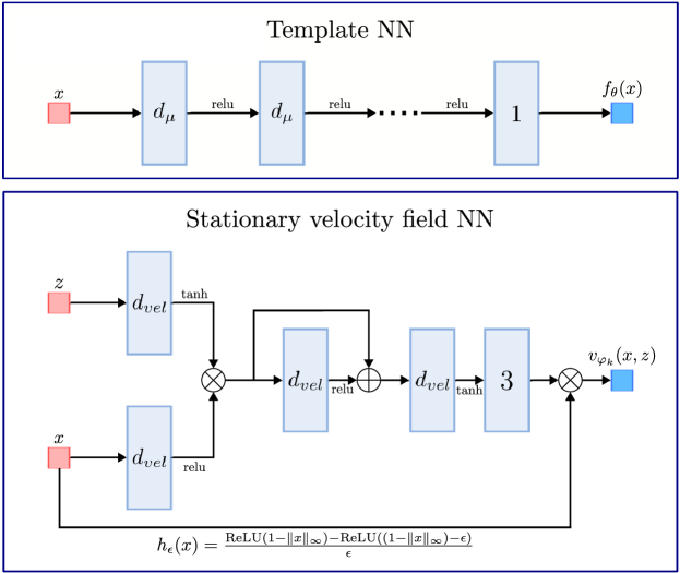
Figure D.1: The architectures for the template neural network $f_{\theta}$ and the stationary velocity vector fields $v_{\varphi_{k}}$. The small red boxes correspond to the latent code input $z$ and the spatial input $x$. Furthermore, the small blue box corresponds to an output, while the rectangles are linear layers with $d_{vel}$ or $d_{\mu}$ output dimensions. Finally, the $\oplus$ and $\otimes$ stand for elementwise addition and scalar/elementwise multiplication, respectively.

Figure D.1 shows the used neural network architectures. For the template neural network, we use nearly the same architecture as the template neural network in [27]. The only difference is that we use ReLU activation functions instead of sine activation functions. In our experiments, we clamp the output of the template neural network to the interval $[-0.5,0.5]$. The stationary velocity vector field neural networks $v_{\varphi_{k}}$ use the architecture in [29]. However, there are some differences. First, we add an extra linear layer at the output. We also add a scalar multiplication with the function $h_{\epsilon}$. This component ensures the velocity vector field is zero outside $\Omega$, which is needed to let the ODE be a diffeomorphism on $\Omega$.

D.2 Pointwise loss

The models by [28] and [29] are similar to our model. However, in contrast to our work, they do not use a Riemannian distance to regularize the time-dependent deformation of the template. Hence, we can not expect a physically plausible deformation that constitutes a geodesic. They use the pointwise regularization given by:

$$L_{pw}=\sum_{t\in T}\sum_{i=1}^{N}\sum_{j=1}^{M}\mathcal{L}_{0.25}\left(\lVert\phi_{i}(p_{j},t)-p_{j}\rVert_{2}\right),$$ (D.1)

where $\mathcal{L}_{0.25}$ is the Huber loss with parameter equal to $0.25$, $T$ is a set of predefined time instances at which to evaluate the pointwise loss, and $\phi_{i}(\cdot,t):=\phi_{t}(\cdot,z_{i})$ with $\frac{\mathrm{d}}{\mathrm{d}t}\phi_{t}(x,z)=v_{\varphi}(\phi_{t}(x,z),t,z)$ and $\phi_{0}(x,z)=x$. For our purposes, we follow [28] and [29] and choose $T=\{\lfloor K/4\rfloor\cdot i\mid 1\leq i\leq K/\lfloor 0.25K\rfloor,i\in\mathbb{N}\}$ with $K$ the number of stationary velocity vector fields in $v_{\varphi}(x,t,z)=\sum_{k=1}^{K}\chi_{[(k-1)/K,k/K]}(t)\cdot v_{\varphi_{k}}(x)$.

In [29], the model uses the above loss to learn a template shape that has similar features to the training shapes. Hence, similar to our Riemannian regularization $\int_{0}^{1}\lVert v\rVert_{V}^{2}\mathrm{d}t$, the pointwise loss is aimed at learning a proper template. Furthermore, note that when choosing $\lVert\cdot\rVert_{V}=\lVert\cdot\rVert_{L_{2}(\Omega)}$, we penalize long curves $x(t)$ defined by $\frac{\mathrm{d}}{\mathrm{d}t}x(t)=v_{\varphi}(x(t),t,z)$. As the pointwise loss penalizes such long curves as well, the pointwise loss can be seen as a non-Riemannian version of our Riemannian integral regularization.

D.3 Datasets

In our work, we use two datasets: a synthetic rectangles dataset and a shape liver dataset [29, 70].

The synthetic rectangles dataset is created by generating random boxes with edge lengths uniformly distributed in $[0.15,0.85]$. Subsequently, these boxes are rotated using a random rotation matrix. For training the point cloud-based model, we sample 100 000 uniform points and corresponding normals from the meshes. For training using the occupancy data (see Section C), we uniformly sample 100 000 points from $\Omega=[-1,1]^{3}$ and calculate the signed distance to the boxes. Subsequently, we calculate the occupancy values from these signed distance values. The training dataset consists of 100 randomly generated parallelograms, while the test dataset consists of 20 parallelograms.

For training the models on the liver dataset, we use the preprocessed data of [29]. The only additional preprocessing step is a scaling of their point cloud data and their mesh data. We multiply the points and the mesh vertices with a scaling factor of $0.75$. This makes sure that all the livers are present in the unit cube. As training data, we sample 100 000 uniform points and corresponding normals from the meshes. Finally, we use the same train-test split as [29], where the training dataset uses 145 samples and the test dataset uses 45 samples.

D.4 Training details

We jointly learn the latent codes $z_{i}$, the template implicit neural representation $f_{\theta}$, and the stationary velocity vector fields $v_{\varphi_{k}}$ ($k\in\{1,\ldots,K\}$). As the template neural network architecture $f_{\theta}$ comes from [27] and the stationary velocity vector fields $v_{\varphi_{k}}$ from [29], we inherit the weight initialization schemes from these works. The latent codes $z_{i}\in\mathbb{R}^{d}$ are initialized by sampling from $\mathcal{N}(0,1/d)$, as in [29].

For each model and dataset pair, we use a batch size of 10 and sample 5000 points for each shape. For the point cloud data, each sample consists of a point lying on the mesh and its corresponding normal. When using the occupancy data, the sampled points lie in $\Omega=[-1,1]^{3}$ and are accompanied by their occupancy value. Half of the points lie inside the shape, while the other half lie outside the shape. Using the sampled points, we can calculate the loss by approximating the expectations via Monte Carlo. In addition, we add an $l_{2}$ penalty on the latent vectors with a regularization constant equal to $10^{-4}$. We update the neural network parameters and the latent codes $z_{i}$ via separate Adam optimizers for the latent codes, the template NN $f_{\theta}$, and velocity field NN $v_{\varphi}$. The initial learning rate for the latent codes is $10^{-3}$, for the $f_{\theta}$ parameters $5\cdot 10^{-4}$, and for the $v_{\varphi}$ parameters $5\cdot 10^{-4}$. Moreover, for each Adam optimizer, we use a learning rate scheduler that multiplies the learning rate with $0.7$ every 250 epochs. Finally, we bound the latent codes $z_{i}$ to be within the unit sphere. For the remainder of the hyperparameters, see Table D.1.

D.5 Inference details

For reconstructing shapes, we solve the following equation:

$$\min_{z}\mathcal{D}_{rec}(\phi_{1}(\cdot,z)^{-1}\cdot\mathcal{T}_{\theta},\mathcal{S})+\gamma\lVert z\rVert_{2}^{2},$$

where

• $\gamma\in\mathbb{R}$,

• $\frac{\mathrm{d}}{\mathrm{d}t}\phi_{t}(x,z)=v_{\varphi}(\phi_{t}(x,z),t,z)$ and $\phi_{0}(x,z)=x$,

• $\mathcal{D}_{rec}(\phi_{1}(\cdot,z)^{-1}\cdot\mathcal{T}_{\theta},\mathcal{S})=\operatorname*{\mathop{\mathbb{E}}}_{x\in\mathcal{S}}\left[\lvert I(x,z,1)\rvert\right]$,

• $I(x,z,t):=((\phi_{t}(\cdot,z))^{-1}\cdot f_{\theta})(x):=f_{\theta}(\phi_{t}(x,z))$.

We solve this optimization problem by running an Adam optimizer with an initial learning rate of $5\cdot 10^{-2}$ for 800 iterations. At iteration 400 the learning rate is decreased by a factor of 10. Furthermore, we put $\gamma=10^{-4}$ and we initialize the latent code from $\mathcal{N}(0,0.01\cdot I)$.

Table D.1: The hyperparameter values every trained model uses on a specific dataset (rectangles or liver). Here $N_{h}$ is the number of linear layers between the first and last linear layer in the template neural network (as presented in Figure D.1). Furthermore, $c_{\text{PW}}$ denotes the regularization constant for the pointwise loss when training the model that uses this loss as the deformation regularizer.

Hyperparameter	Value (Rect.)	Value (Liver)
Epochs	4000	3000
Latent dimension	32	32
$d_{vel}$	512	512
$d_{\mu}$	256	256
$\epsilon$	0.05	0.05
$K$	10	10
$d_{\mu}$	256	256
$N_{h}$	5	5
$\sigma^{2}$	0.025	0.002
$\tau$	0.01	0.01
$\lambda$	0.005	0.005
$\beta$	1.5	1.5
$\alpha$	100	100
$\eta$	0.05	50
$c_{\text{PW}}$	0.1	0.1

References

- [1] Chong Chen and Ozan Öktem. Indirect image registration with large diffeomorphic deformations. SIAM Journal on Imaging Sciences, 11(1):575–617, 2018.
- [2] Lukas F. Lang, Sebastian Neumayer, Ozan Öktem, and Carola-Bibiane Schönlieb. Template-Based Image Reconstruction from Sparse Tomographic Data. Applied Mathematics & Optimization, 82(3):1081–1109, 2020.
- [3] Jiulong Liu, Angelica I. Aviles-Rivero, Hui Ji, and Carola-Bibiane Schönlieb. Rethinking medical image reconstruction via shape prior, going deeper and faster: Deep joint indirect registration and reconstruction. Medical Image Analysis, 68:101930, 2021.
- [4] Chong Chen, Barbara Gris, and Ozan Öktem. A new variational model for joint image reconstruction and motion estimation in spatiotemporal imaging. SIAM Journal on Imaging Sciences, 12(4):1686–1719, 2019.
- [5] Andreas Hauptmann, Ozan Öktem, and Carola Schönlieb. Image Reconstruction in Dynamic Inverse Problems with Temporal Models, pages 1–31. Springer International Publishing, Cham, 2021.
- [6] M Faisal Beg, Michael I Miller, Alain Trouvé, and Laurent Younes. Computing large deformation metric mappings via geodesic flows of diffeomorphisms. International Journal of Computer Vision, 61(2):139–157, 2005.
- [7] Marc Vaillant and Joan Glaunès. Surface matching via currents. In International Conference on Information Processing in Medical Imaging, pages 381–392. Springer, 2005.
- [8] Michael I Miller, Alain Trouvé, and Laurent Younes. Geodesic shooting for computational anatomy. Journal of Mathematical Imaging and Vision, 24:209–228, 2006.
- [9] François-Xavier Vialard, Laurent Risser, Daniel Rueckert, and Colin J Cotter. Diffeomorphic 3d image registration via geodesic shooting using an efficient adjoint calculation. International Journal of Computer Vision, 97:229–241, 2012.
- [10] Laurent Younes. Shapes and Diffeomorphisms. Springer, 2 edition, 2019.
- [11] Miaomiao Zhang and P Thomas Fletcher. Fast diffeomorphic image registration via fourier-approximated lie algebras. International Journal of Computer Vision, 127:61–73, 2019.
- [12] Boulbaba Ben Amor, Sylvain Arguillere, and Ling Shao. Resnet-lddmm: Advancing the lddmm framework using deep residual networks. IEEE Transactions on Pattern Analysis and Machine Intelligence, 45(3):3707–3720, 2022.
- [13] Sarang Joshi, Brad Davis, Matthieu Jomier, and Guido Gerig. Unbiased diffeomorphic atlas construction for computational anatomy. NeuroImage, 23:S151–S160, 2004.
- [14] Jun Ma, Michael I Miller, Alain Trouvé, and Laurent Younes. Bayesian template estimation in computational anatomy. NeuroImage, 42(1):252–261, 2008.
- [15] Jun Ma, Michael I Miller, and Laurent Younes. A bayesian generative model for surface template estimation. International Journal of Biomedical Imaging, 2010:1–14, 2010.
- [16] Balder Croquet, Daan Christiaens, Seth M Weinberg, Michael Bronstein, Dirk Vandermeulen, and Peter Claes. Unsupervised diffeomorphic surface registration and non-linear modelling. In International Conference on Medical Image Computing and Computer Assisted Intervention (MICCAI), pages 118–128. Springer, 2021.
- [17] Marvin Eisenberger, David Novotny, Gael Kerchenbaum, Patrick Labatut, Natalia Neverova, Daniel Cremers, and Andrea Vedaldi. Neuromorph: Unsupervised shape interpolation and correspondence in one go. In Proceedings of the IEEE/CVF Conference on Computer Vision and Pattern Recognition (CVPR), pages 7473–7483, 2021.
- [18] Qixing Huang, Xiangru Huang, Bo Sun, Zaiwei Zhang, Junfeng Jiang, and Chandrajit Bajaj. Arapreg: An as-rigid-as possible regularization loss for learning deformable shape generators. In Proceedings of the IEEE/CVF International Conference on Computer Vision, pages 5815–5825, 2021.
- [19] Kunal Gupta and Manmohan Chandraker. Neural mesh flow: 3d manifold mesh generation via diffeomorphic flows. In Advances in Neural Information Processing Systems, volume 33, pages 1747–1758. Curran Associates, Inc., 2020.
- [20] Luca Cosmo, Antonio Norelli, Oshri Halimi, Ron Kimmel, and Emanuele Rodola. Limp: Learning latent shape representations with metric preservation priors. In European Conference on Computer Vision, pages 19–35. Springer, 2020.
- [21] Elena Balashova, Jiangping Wang, Vivek Singh, Bogdan Georgescu, Brian Teixeira, and Ankur Kapoor. 3d organ shape reconstruction from topogram images. In International Conference on Information Processing in Medical Imaging, pages 347–359. Springer, 2019.
- [22] Katarína Tóthová, Sarah Parisot, Matthew Lee, Esther Puyol-Antón, Andrew King, Marc Pollefeys, and Ender Konukoglu. Probabilistic 3d surface reconstruction from sparse mri information. In International Conference on Medical Image Computing and Computer Assisted Intervention (MICCAI), pages 813–823. Springer, 2020.
- [23] David Wiesner, Julian Suk, Sven Dummer, David Svoboda, and Jelmer M Wolterink. Implicit neural representations for generative modeling of living cell shapes. In International Conference on Medical Image Computing and Computer Assisted Intervention (MICCAI), pages 58–67. Springer, 2022.
- [24] Jeong Joon Park, Peter Florence, Julian Straub, Richard Newcombe, and Steven Lovegrove. Deepsdf: Learning continuous signed distance functions for shape representation. In Proceedings of the IEEE/CVF Conference on Computer Vision and Pattern Recognition (CVPR), pages 165–174, 2019.
- [25] Vincent Sitzmann, Julien Martel, Alexander Bergman, David Lindell, and Gordon Wetzstein. Implicit neural representations with periodic activation functions. In Advances in Neural Information Processing Systems, volume 33, pages 7462–7473. Curran Associates, Inc., 2020.
- [26] Lars Mescheder, Michael Oechsle, Michael Niemeyer, Sebastian Nowozin, and Andreas Geiger. Occupancy networks: Learning 3d reconstruction in function space. In Proceedings of the IEEE/CVF Conference on Computer Vision and Pattern Recognition (CVPR), pages 4460–4470, 2019.
- [27] Yu Deng, Jiaolong Yang, and Xin Tong. Deformed implicit field: Modeling 3d shapes with learned dense correspondence. In Proceedings of the IEEE/CVF Conference on Computer Vision and Pattern Recognition (CVPR), pages 10286–10296, 2021.
- [28] Zerong Zheng, Tao Yu, Qionghai Dai, and Yebin Liu. Deep implicit templates for 3d shape representation. In Proceedings of the IEEE/CVF Conference on Computer Vision and Pattern Recognition (CVPR), pages 1429–1439, 2021.
- [29] Shanlin Sun, Kun Han, Deying Kong, Hao Tang, Xiangyi Yan, and Xiaohui Xie. Topology-preserving shape reconstruction and registration via neural diffeomorphic flow. In Proceedings of the IEEE/CVF Conference on Computer Vision and Pattern Recognition (CVPR), pages 20845–20855, 2022.
- [30] Matan Atzmon, David Novotny, Andrea Vedaldi, and Yaron Lipman. Augmenting implicit neural shape representations with explicit deformation fields. arXiv preprint arXiv:2108.08931, 2021.
- [31] Christopher M Bishop and Nasser M Nasrabadi. Pattern recognition and machine learning. Springer, 2006.
- [32] P Thomas Fletcher, Conglin Lu, Stephen M Pizer, and Sarang Joshi. Principal geodesic analysis for the study of nonlinear statistics of shape. IEEE Transactions on Medical Imaging, 23(8):995–1005, 2004.
- [33] Miaomiao Zhang and Tom Fletcher. Probabilistic principal geodesic analysis. In Advances in Neural Information Processing Systems, volume 26, page 1178–1186. Curran Associates, Inc., 2013.
- [34] Martial Agueh and Guillaume Carlier. Barycenters in the wasserstein space. SIAM Journal on Mathematical Analysis, 43(2):904–924, 2011.
- [35] Vivien Seguy and Marco Cuturi. Principal geodesic analysis for probability measures under the optimal transport metric. In Advances in Neural Information Processing Systems, volume 28, pages 3312–3320. Curran Associates, Inc., 2015.
- [36] Miaomiao Zhang and P Thomas Fletcher. Bayesian principal geodesic analysis for estimating intrinsic diffeomorphic image variability. Medical Image Analysis, 25(1):37–44, 2015.
- [37] Miaomiao Zhang, William M Wells III, and Polina Golland. Probabilistic modeling of anatomical variability using a low dimensional parameterization of diffeomorphisms. Medical Image Analysis, 41:55–62, 2017.
- [38] Behrend Heeren, Chao Zhang, Martin Rumpf, and William Smith. Principal geodesic analysis in the space of discrete shells. Computer Graphics Forum, 37(5):173–184, 2018.
- [39] Marc Vaillant, Michael I Miller, Laurent Younes, and Alain Trouvé. Statistics on diffeomorphisms via tangent space representations. NeuroImage, 23:S161–S169, 2004.
- [40] Benjamin Charlier, Jean Feydy, David W Jacobs, and Alain Trouvé. Distortion minimizing geodesic subspaces in shape spaces and computational anatomy. In VipIMAGE 2017, pages 1135–1144. Springer, 2018.
- [41] Nina Miolane and Susan Holmes. Learning weighted submanifolds with variational autoencoders and riemannian variational autoencoders. In Proceedings of the IEEE/CVF Conference on Computer Vision and Pattern Recognition (CVPR), pages 14503–14511, 2020.
- [42] Alexandre Bône, Maxime Louis, Olivier Colliot, Stanley Durrleman, Alzheimer’s Disease Neuroimaging Initiative, et al. Learning low-dimensional representations of shape data sets with diffeomorphic autoencoders. In International Conference on Information Processing in Medical Imaging, pages 195–207. Springer, 2019.
- [43] Georgios Arvanitidis, Lars Kai Hansen, and Søren Hauberg. Latent space oddity: on the curvature of deep generative models. arXiv preprint arXiv:1710.11379, 2017.
- [44] Georgios Arvanitidis, Soren Hauberg, Philipp Hennig, and Michael Schober. Fast and robust shortest paths on manifolds learned from data. In Proceedings of the Twenty-Second International Conference on Artificial Intelligence and Statistics, volume 89 of Proceedings of Machine Learning Research, pages 1506–1515. PMLR, 2019.
- [45] Nutan Chen, Alexej Klushyn, Richard Kurle, Xueyan Jiang, Justin Bayer, and Patrick Smagt. Metrics for deep generative models. In Proceedings of the Twenty-First International Conference on Artificial Intelligence and Statistics, volume 84 of Proceedings of Machine Learning Research, pages 1540–1550. PMLR, 2018.
- [46] Clément Chadebec, Clément Mantoux, and Stéphanie Allassonnière. Geometry-aware hamiltonian variational auto-encoder. arXiv preprint arXiv:2010.11518, 2020.
- [47] Georgios Arvanitidis, Bogdan M. Georgiev, and Bernhard Schölkopf. A prior-based approximate latent riemannian metric. In Proceedings of The 25th International Conference on Artificial Intelligence and Statistics, volume 151 of Proceedings of Machine Learning Research, pages 4634–4658. PMLR, 2022.
- [48] Cong Geng, Jia Wang, Li Chen, Wenbo Bao, Chu Chu, and Zhiyong Gao. Uniform interpolation constrained geodesic learning on data manifold. arXiv preprint arXiv:2002.04829, 2020.
- [49] Tao Yang, Georgios Arvanitidis, Dongmei Fu, Xiaogang Li, and Søren Hauberg. Geodesic clustering in deep generative models. arXiv preprint arXiv:1809.04747, 2018.
- [50] Clément Chadebec and Stéphanie Allassonnière. Data augmentation with variational autoencoders and manifold sampling. In Deep Generative Models, and Data Augmentation, Labelling, and Imperfections, pages 184–192. Springer, 2021.
- [51] Ricky TQ Chen, Yulia Rubanova, Jesse Bettencourt, and David K Duvenaud. Neural ordinary differential equations. In Advances in Neural Information Processing Systems, volume 31, page 6572–6583. Curran Associates, Inc., 2018.
- [52] Samuel Greydanus, Misko Dzamba, and Jason Yosinski. Hamiltonian neural networks. In Advances in Neural Information Processing Systems, volume 32, pages 15379–15389. Curran Associates, Inc., 2019.
- [53] Yaofeng Desmond Zhong, Biswadip Dey, and Amit Chakraborty. Symplectic ode-net: Learning hamiltonian dynamics with control. arXiv preprint arXiv:1909.12077, 2019.
- [54] Miles Cranmer, Sam Greydanus, Stephan Hoyer, Peter Battaglia, David Spergel, and Shirley Ho. Lagrangian neural networks. arXiv preprint arXiv:2003.04630, 2020.
- [55] Alexander Tong, Jessie Huang, Guy Wolf, David Van Dijk, and Smita Krishnaswamy. TrajectoryNet: A dynamic optimal transport network for modeling cellular dynamics. In Proceedings of the 37th International Conference on Machine Learning, volume 119 of Proceedings of Machine Learning Research, pages 9526–9536. PMLR, 2020.
- [56] Derek Onken, Levon Nurbekyan, Xingjian Li, Samy Wu Fung, Stanley Osher, and Lars Ruthotto. A neural network approach for high-dimensional optimal control applied to multiagent path finding. IEEE Transactions on Control Systems Technology, 31(1):235–251, 2023.
- [57] Yannik Wotte, Sven Dummer, Nicolò Botteghi, Christoph Brune, Stefano Stramigioli, and Federico Califano. Discovering efficient periodic behaviours in mechanical systems via neural approximators. arXiv preprint arXiv:2212.14253, 2022.
- [58] Liu Yang and George Em Karniadakis. Potential flow generator with l2 optimal transport regularity for generative models. IEEE Transactions on Neural Networks and Learning Systems, 33(2):528–538, 2022.
- [59] Michael Niemeyer, Lars Mescheder, Michael Oechsle, and Andreas Geiger. Occupancy flow: 4d reconstruction by learning particle dynamics. In Proceedings of the IEEE/CVF International Conference on Computer Vision (ICCV), pages 5379–5389, 2019.
- [60] Jean-David Benamou and Yann Brenier. A computational fluid mechanics solution to the monge-kantorovich mass transfer problem. Numerische Mathematik, 84(3):375–393, 2000.
- [61] Lars Ruthotto, Stanley J Osher, Wuchen Li, Levon Nurbekyan, and Samy Wu Fung. A machine learning framework for solving high-dimensional mean field game and mean field control problems. Proceedings of the National Academy of Sciences, 117(17):9183–9193, 2020.
- [62] Chris Finlay, Joern-Henrik Jacobsen, Levon Nurbekyan, and Adam Oberman. How to train your neural ODE: the world of Jacobian and kinetic regularization. In Proceedings of the 37th International Conference on Machine Learning, volume 119 of Proceedings of Machine Learning Research, pages 3154–3164. PMLR, 2020.
- [63] Derek Onken, Samy Wu Fung, Xingjian Li, and Lars Ruthotto. Ot-flow: Fast and accurate continuous normalizing flows via optimal transport. Proceedings of the AAAI Conference on Artificial Intelligence, 35(10):9223–9232, 2021.
- [64] William E. Lorensen and Harvey E. Cline. Marching cubes: A high resolution 3d surface construction algorithm. SIGGRAPH Comput. Graph., 21(4):163–169, 1987.
- [65] Paul Dupuis, Ulf Grenander, and Michael I Miller. Variational problems on flows of diffeomorphisms for image matching. Quarterly of applied mathematics, 56(3):587–600, 1998.
- [66] Mirza Faisal Beg and Ali Khan. Computing an average anatomical atlas using lddmm and geodesic shooting. In 3rd IEEE International Symposium on Biomedical Imaging: Nano to Macro, pages 1116–1119. IEEE, 2006.
- [67] Amos Gropp, Lior Yariv, Niv Haim, Matan Atzmon, and Yaron Lipman. Implicit geometric regularization for learning shapes. In International Conference on Machine Learning, pages 3789–3799. PMLR, 2020.
- [68] Justin Solomon, Mirela Ben-Chen, Adrian Butscher, and Leonidas Guibas. As-killing-as-possible vector fields for planar deformation. Computer Graphics Forum, 30(5):1543–1552, 2011.
- [69] Michael Tao, Justin Solomon, and Adrian Butscher. Near-isometric level set tracking. Computer Graphics Forum, 35(5):65–77, 2016.
- [70] Xuming Chen, Shanlin Sun, Narisu Bai, Kun Han, Qianqian Liu, Shengyu Yao, Hao Tang, Chupeng Zhang, Zhipeng Lu, Qian Huang, et al. A deep learning-based auto-segmentation system for organs-at-risk on whole-body computed tomography images for radiation therapy. Radiotherapy and Oncology, 160:175–184, 2021.
- [71] David Lüdke, Tamaz Amiranashvili, Felix Ambellan, Ivan Ezhov, Bjoern H Menze, and Stefan Zachow. Landmark-free statistical shape modeling via neural flow deformations. In Medical Image Computing and Computer Assisted Intervention (MICCAI), pages 453–463. Springer, 2022.
- [72] Benedikt Wirth, Leah Bar, Martin Rumpf, and Guillermo Sapiro. A continuum mechanical approach to geodesics in shape space. International Journal of Computer Vision, 93:293–318, 2011.
- [73] Martin Rumpf and Benedikt Wirth. Discrete geodesic calculus in shape space and applications in the space of viscous fluidic objects. SIAM Journal on Imaging Sciences, 6(4):2581–2602, 2013.
- [74] Otmar Scherzer. Handbook of mathematical methods in imaging. Springer, 2010.
- [75] Jürgen Jost. Riemannian geometry and geometric analysis. Springer, 7 edition, 2017.