Variance Decay Property for Filter Stability

Abstract

This paper is concerned with the problem of nonlinear (stochastic) filter stability of a hidden Markov model (HMM) with white noise observations. A contribution is the variance decay property which is used to conclude filter stability. For this purpose, a new notion of the Poincaré inequality (PI) is introduced for the nonlinear filter. PI is related to both the ergodicity of the Markov process as well as the observability of the HMM. The proofs are based upon a recently discovered minimum variance duality which is used to transform the nonlinear filtering problem into a stochastic optimal control problem for a backward stochastic differential equation (BSDE).

Nonlinear filtering; Optimal control; Stochastic systems.

1 Introduction

This paper is on the topic of nonlinear (stochastic) filter stability – in the sense of asymptotic forgetting of the initial condition. The results are described for the continuous-time hidden Markov model (HMM) with white noise observations. The novelty comes from the methodological aspects which here are based on the minimum variance duality introduced in our prior work: dual characterization of stochastic observability presented in [1]; and the dual optimal control problem described in [2]. In the present paper, these are used to investigate the question of nonlinear filter stability,

1.1 Literature review of filter stability

While duality is central to the stability analysis of the Kalman filter and also in the study of deterministic minimum energy estimator (MEE) [3], with the sole exception of van Handel’s PhD thesis [4], duality is absent in stochastic filter stability theory. Viewed from a certain lens, the story of filter stability is a story of two parts: (i) Stability of the Kalman filter where dual (control-theoretic) definitions and methods are paramount; and (ii) Stability of the nonlinear filter where there is little hint of such methods.

The disconnect is already seen in the earliest works – in the two parts of the pioneering 1996 paper of Ocone and Pardoux [5] on the topic of filter stability. The paper is divided into two parts: Sec. 2 of the paper considers the linear Gaussian model and the Sec. 3 considers the nonlinear models (HMM). While the problem is the same, the definitions, tools and techniques of the two sections have no overlap. In [5, Sec. 2], there are several control-theoretic definitions given, optimal control techniques employed for analysis, references cited, while in [5, Sec. 3] there are none. The passage of time did not change matters much: In his award winning 2010 MTNS review paper, van Handel writes “The proofs of the Kalman filter results are of essentially no use [for nonlinear filter stability], so we must start from scratch [6].”

Our paper is the first time that such a complete generalization of the linear Gaussian results has been possible based on the use of duality. A summary of the two main contributions is described as part of Sec. 1.2 after the literature review.

The problem of nonlinear filter stability is far from straightforward. In fact, [5, Sec. 3] is based on some prior work of Kunita [7] which was later found to contain a gap, as discussed in some detail in [8] (see also [9, Sec. 6.2]). The gap also served to invalidate the main result in [5, Sec. 3]. The literature on filter stability is divided into two cases:

• The case where the Markov process forgets the prior and therefore the filter “inherits” the same property;

• The case where the observation provides sufficient information about the hidden state, allowing the filter to correct its erroneous initialization.

These two cases are referred to as the ergodic and non-ergodic signal cases, respectively. While the two cases are intuitively reasonable, they spurred much work during 1990-2010 with a complete resolution appearing only at the end of this time-period. See [10, 11] for a comprehensive survey of the filter stability problem including some of this historical context.

For the ergodic signal case, apart from the pioneering contribution [5], early work is based on contraction analysis of the random matrix products arising from recursive application of the Bayes’ formula [12] (see also [13, Ch. 4.3]). The analysis of the Duncan-Mortensen-Zakai (DMZ) equation leads to useful formulae for the Lyapunov exponents under assumptions on model parameters and noise limits [14], and convergence rate estimates are obtained using Feynman-Kac type representation [15]. A comprehensive account for the ergodic signal case appears in [16] and the first complete solution appeared in [8].

For the non-ergodic signal case, a notable early contribution is [17] where a formula for the relative entropy is derived. It is shown that the relative entropy is a Lyapunov function for the filter (see Rem. 3.6). Notable also is the partial differential equation (PDE) approach of [18, 19] where sufficient conditions for filter stability are described for a certain class of HMMs on the Euclidean state-space with linear observations (see also [4, Ch. 4]). Our own prior work [20] is closely inspired by [8] who were the first to formulate certain observability-type “identifying conditions” for the HMM on finite state-space. These conditions were formulated in terms of the HMM model parameters and shown to be sufficient for the stability of the Wonham filter.

For a general class of HMMs, the fundamental definition for stochastic observability and detectability is due to van Handel [21, 22]. There are two notable features: (i) the definition made rigorous the intuition described in the two cases [6, Sec. II-B and Sec. V]; and (ii) the definition led to meaningful conditions that were shown to be necessary and sufficient for filter stability [6, Thm. III.3 and Thm. V.2]. The proof techniques are broadly referred to as the intrinsic approach. In [11], the authors explain “By ‘intrinsic’ we mean methods which directly exploit the fundamental representation of the filter as a conditional expectation through classical probabilistic techniques.” Recent extensions and refinements of these can be found in [23, 24, 25].

A thorough mathematical review of these past approaches to the problem of filter stability appears in the PhD thesis of the first author [9, Ch. 6]. Additional mathematical comparisons with the approach of the present paper appear as part of Remarks 3.4-3.6 in Sec. 3.1 and Table 4 in Appendix A.2.

1.2 Summary of original contributions

The two main contributions are as follows:

1. The paper introduces a new notion of Poincaré inequality (PI) for the nonlinear filter. The PI is used to obtain a novel formula for the filter stability (Thm. 5.19).

2. PI is related to the two model properties, namely, the observability of the HMM (Prop. 6.32), and the ergodicity of the signal model (Prop. 6.36).

A key contribution is the variance decay property (Eq. (6)). The property at once unifies and generalizes two bodies of results where the notion is variance is important:

• Stability analysis of the Kalman filter: The notion of variance is the conditional covariance (also referred to as the error covariance), which recall is given by the solution of the DRE.

• Stochastic stability: The notion of variance is related to the Poincaré inequality (PI) which is a standard assumption to conclude asymptotic stability of a Markov process (without conditioning).

This paper builds upon the research conducted in the PhD thesis of the first author [9]. On the topic of filter stability, two conference papers have previously been published by our group [26, 20]. Both these prior papers were drawn from the PhD thesis. Most closely related is [26] where the concept of conditional PI was first introduced. The concept is discussed as Rem. 5.29 in the present paper.

It is important to note that all of the results presented in this paper are original and distinct from our previous papers. Moreover, the two central concepts in this paper – the backward map (4) and the variance decay property (6) – are both original. Notably, the backward map is useful to connect our work to the intrinsic approach to filter stability (Rem. 3.5).

1.3 Outline

The outline of the remainder of this paper is as follows. The mathematical background on HMMs and the filter stability problem appears in Sec. 2. The two central concepts in this paper – the backward map and the variance decay property – are introduced in Sec. 3. Sec. 4 contains a discussion of function spaces and the dual optimal control problem. This is followed by two sections that describes the two main contributions: Sec. 5 introduces the Poincaré inequality and Sec. 6 describes its relationship to the HMM model properties. Sec. 7 contains some numerical examples showing the significance of the Poincaré constant to convergence rate for the filter. The paper closes with some conclusions and directions for future work in Sec. 8. Details of the proofs appear in the Appendix.

2 Math Preliminaries and problem statement

2.1 Hidden Markov model

HMM: On the probability space $(\Omega,{\cal F}_{T},{\sf P})$, consider a pair of continuous-time stochastic processes $(X,Z)$ as follows:

• The state process $X=\{X_{t}:\Omega\to\mathbb{S}:0\leq t\leq T\}$ is a Feller-Markov process taking values in the state-space $\mathbb{S}$ which is assumed to be a locally compact Polish space. The prior is denoted by $\mu\in{\cal P}(\mathbb{S})$ (where ${\cal P}(\mathbb{S})$ is the space of probability measures defined on the Borel $\sigma$-algebra on $\mathbb{S}$) and $X_{0}\sim\mu$. The infinitesimal generator of $X$ is denoted by ${\cal A}$.

• The observation process $Z=\{Z_{t}:0\leq t\leq T\}$ satisfies the stochastic differential equation (SDE):

  $$Z_{t}=\int_{0}^{t}h(X_{s})\,\mathrm{d}s+W_{t},\quad t\geq 0$$ (1)

  where $h:\mathbb{S}\to\mathbb{R}^{m}$ is referred to as the observation function and $W=\{W_{t}:0\leq t\leq T\}$ is an $m$-dimensional Brownian motion (B.M.). We write $W$ is ${\sf P}$-B.M. It is assumed that $W$ is independent of $X$. The filtration generated by the observation is denoted by ${\cal Z}:=\{{\cal Z}_{t}:0\leq t\leq T\}$ where ${\cal Z}_{t}=\sigma\big{(}\{Z_{s}:0\leq s\leq t\}\big{)}$.

The above is referred to as the white noise observation model of nonlinear filtering. The model is denoted by $({\cal A},h)$. For reasons of well-posedness, the model requires additional technical conditions. In lieu of stating these conditions for general class of HMMs, we restrict our study to the examples described in the following:

Example 1 (Examples of state processes)

The two examples are as follows:

• $\mathbb{S}=\{1,2,\ldots,d\}$. A real-valued function $f$ is identified with a vector in $\mathbb{R}^{d}$ where the $x-{\text{th}}$ element of the vector is $f(x)$ for $x\in\mathbb{S}$. Based on this, the observation function $h$ is a $d\times m$ matrix and the generator ${\cal A}$ is a $d\times d$ transition rate matrix, whose $(x,y)$ entry (for $x,y\in\mathbb{S}$ and $x\neq y$) is the positive rate of transition from $x\mapsto y$ and ${\cal A}(x,x)=-\sum_{y:y\neq x}{\cal A}(x,y)$.

• $\mathbb{S}\subseteq\mathbb{R}^{d}$. $X$ is an Itô diffusion process defined by:

  $$\,\mathrm{d}X_{t}=a(X_{t})\,\mathrm{d}t+\sigma(X_{t})\,\mathrm{d}B_{t},\quad X_{0}\sim\mu$$ (2)

  where $a(\cdot)$ and $\sigma(\cdot)$ are given $C^{1}$ smooth functions that satisfy linear growth conditions at $\infty$. The infinitesimal generator ${\cal A}$ is given by [27, Thm. 7.3.3]

  $$({\cal A}f)(x)=a^{\hbox{\rm\tiny T}}(x)\nabla f(x)+{\mathchoice{\genfrac{}{}{}{1}{1}{2}}{\genfrac{}{}{}{2}{1}{2}}{\genfrac{}{}{}{3}{1}{2}}{\genfrac{}{}{}{4}{1}{2}}}\mbox{tr}\big{(}\sigma\sigma^{\hbox{\rm\tiny T}}(x)(D^{2}f)(x)\big{)},\;x\in\mathbb{S}$$

  where $\nabla f$ and $D^{2}f$ are the gradient vector and the Hessian matrix, respectively, of the function $f\in C^{2}(\mathbb{R}^{d})$.

• The linear Gaussian model is the special case of an Itô diffusion where the drift $a(\cdot)$ is linear, $\sigma$ is a constant matrix, and the prior $\mu$ is a Gaussian density.

Remark 1

Of the two models of state processes, the HMM on a finite state-space is of the most interest. We continue to use the notation $({\cal A},h)$ and state the results in their general form with the understanding that, for the general class of HMMs, the calculations are formal.

Nonlinear filter: The objective of nonlinear (or stochastic) filtering is to compute the conditional expectation

$$\pi_{T}(f):={\sf E}\big{(}f(X_{T})\mid{\cal Z}_{T}\big{)},\quad f\in C_{b}(\mathbb{S})$$

where $C_{b}(\mathbb{S})$ is the space of continuous and bounded functions. The conditional expectation is referred to as the nonlinear filter. Assuming a certain technical (Novikov’s) condition holds, the nonlinear filter solves the Kushner-Stratonovich equation:

$$\,\mathrm{d}\pi_{t}(f)=\pi_{t}({\cal A}f)\,\mathrm{d}t+\big{(}\pi_{t}(hf)-\pi_{t}(f)\pi_{t}(h)\big{)}^{\hbox{\rm\tiny T}}\,\mathrm{d}I_{t}$$ (3)

with $\pi_{0}=\mu$ where the innovation process is defined by

$$I_{t}:=Z_{t}-\int_{0}^{t}\pi_{s}(h)\,\mathrm{d}s,\quad t\geq 0$$

With $h=c{\sf 1}$, the coefficient of $\,\mathrm{d}I_{t}$ in (3) is zero and $\{\pi_{t}:t\geq 0\}$ becomes a deterministic process. The resulting evolution equation is referred to as the forward Kolmogorov equation.

2.2 Filter stability: Definitions and metrics

Let $\rho\in{\cal P}(\mathbb{S})$. On the common measurable space $(\Omega,{\cal F}_{T})$, ${\sf P}^{\rho}$ is used to denote another probability measure such that the transition law of $(X,Z)$ is identical but $X_{0}\sim\rho$ (see [17, Sec. 2.2] for an explicit construction of ${\sf P}^{\rho}$ as a probability measure over the space of the trajectories of the process $(X,Z)$.). The associated expectation operator is denoted by ${\sf E}^{\rho}(\cdot)$ and the nonlinear filter by $\pi_{t}^{\rho}(f)={\sf E}^{\rho}\big{(}f(X_{t})|{\cal Z}_{t}\big{)}$. It solves (3) with $\pi_{0}=\rho$. The two most important choices for $\rho$ are as follows:

• $\rho=\mu$. The measure $\mu$ has the meaning of the true prior.

• $\rho=\nu$. The measure $\nu$ has the meaning of the incorrect prior that is used to compute the filter by solving (3) with $\pi_{0}=\nu$. It is assumed that $\mu\ll\nu$.

The relationship between ${\sf P}^{\mu}$ and ${\sf P}^{\nu}$ is as follows (${\sf P}^{\mu}|_{{\cal Z}_{t}}$ denotes the restriction of ${\sf P}^{\mu}$ to the $\sigma$-algebra ${\cal Z}_{t}$):

Lemma 1 (Lemma 2.1 in [17])

Suppose $\mu\ll\nu$. Then

• ${\sf P}^{\mu}\ll{\sf P}^{\nu}$, and the change of measure is given by

  $$\frac{\,\mathrm{d}{\sf P}^{\mu}}{\,\mathrm{d}{\sf P}^{\nu}}(\omega)=\frac{\,\mathrm{d}\mu}{\,\mathrm{d}\nu}\big{(}X_{0}(\omega)\big{)}\quad{\sf P}^{\nu}\text{-a.s.}\;\omega$$

• For each $t>0$, $\pi_{t}^{\mu}\ll\pi_{t}^{\nu}$, ${\sf P}^{\mu}|_{{\cal Z}_{t}}$-a.s..

The following definition of filter stability is based on $f$-divergence (Because $\mu$ has the meaning of the correct prior, the expectation is with respect to ${\sf P}^{\mu}$):

Definition 1

The nonlinear filter is stable in the sense of

(KL divergence) $${\sf E}^{\mu}\big{(}{\sf D}(\pi_{T}^{\mu}\mid\pi_{T}^{\nu})\big{)}\;\longrightarrow\;0$$

($$\chi^{2} {\sf E}^{\mu}\big{(}{\chi^{2}}(\pi_{T}^{\mu}\mid\pi_{T}^{\nu})\big{)}\;\longrightarrow\;0$$ divergence)

(Total variation) $${\sf E}^{\mu}\big{(}\|\pi_{T}^{\mu}-\pi_{T}^{\nu}\|_{\text{\tiny TV}}\big{)}\;\longrightarrow\;0$$

as $T\to\infty$ for every $\mu,\nu\in{\cal P}(\mathbb{S})$ such that $\mu\ll\nu$. (See Appendix A.1 for definitions of the $f$-divergence).

Apart from $f$-divergence based definitions, the following definitions of filter stability are also of historical interest:

Definition 2

The nonlinear filter is stable in the sense of

($$L^{2} {\sf E}^{\mu}\big{(}|\pi_{T}^{\mu}(f)-\pi_{T}^{\nu}(f)|^{2}\big{)}\;\longrightarrow\;0$$)

(a.s.) $$|\pi_{T}^{\mu}(f)-\pi_{T}^{\nu}(f)|\;\longrightarrow\;0\quad{\sf P}^{\mu}\text{-a.s.}$$

as $T\to\infty$, for every $f\in C_{b}(\mathbb{S})$ and $\mu,\nu\in{\cal P}(\mathbb{S})$ s.t. $\mu\ll\nu$.

In this paper, our objective is to prove filter stability in the sense of ${\chi^{2}}$-divergence. Based on well known relationship between f-divergences, this also implies other types of stability as follows:

Proposition 1

If the filter is stable in the sense of ${\chi^{2}}$ then it is stable in KL divergence, total variation, and $L^{2}$.

Proof 2.1.

See Appendix A.1.

Because these were stated piecemeal, the main assumptions are stated formally as follows:

Assumption 0: Consider HMM $({\cal A},h)$.

1. $\mu,\nu\in{\cal P}(\mathbb{S})$ are two priors with $\mu\ll\nu$.

2. Novikov’s condition holds:

   $${\sf E}\left(\exp\big{(}{\mathchoice{\genfrac{}{}{}{1}{1}{2}}{\genfrac{}{}{}{2}{1}{2}}{\genfrac{}{}{}{3}{1}{2}}{\genfrac{}{}{}{4}{1}{2}}}\int_{0}^{\tau}|h(X_{t})|^{2}\,\mathrm{d}t\big{)}\right)<\infty$$

   The condition holds, e.g., if $h\in C_{b}(\mathbb{S})$.

3. The generator ${\cal A}$ is for one of the two models introduced in Example 1.

3 Main idea: Backward map and variance decay

Suppose $\mu\ll\nu$. Denote

$$\gamma_{T}(x):=\frac{\,\mathrm{d}\pi_{T}^{\mu}}{\,\mathrm{d}\pi_{T}^{\nu}}(x),\quad x\in\mathbb{S}$$

It is well-defined because $\pi_{T}^{\mu}\ll\pi_{T}^{\nu}$ from Lem. 1 (we adopt here the convention that $\frac{0}{0}=0$). It is noted that while $\gamma_{0}=\frac{\,\mathrm{d}\mu}{\,\mathrm{d}\nu}$ is deterministic, $\gamma_{T}$ is a ${\cal Z}_{T}$-measurable function on $\mathbb{S}$. Both of these are examples of likelihood ratio and referred to as such throughout the paper.

A key original concept introduced in this paper is the backward map $\gamma_{T}\mapsto y_{0}$ defined as follows:

$$y_{0}(x):={\sf E}^{\nu}(\gamma_{T}(X_{T})|[X_{0}=x]),\quad x\in\mathbb{S}$$ (4)

The function $y_{0}:\mathbb{S}\to\mathbb{R}$ is deterministic, non-negative, and $\nu(y_{0})={\sf E}^{\nu}(\gamma_{T}(X_{T}))=1$, and therefore is also a likelihood ratio. The significance of this map to the problem of filter stability comes from the following proposition:

Proposition 3.2.

Consider the backward map $\gamma_{T}\mapsto y_{0}$ defined by (4). Then

$$|{\sf E}^{\mu}\big{(}\chi^{2}(\pi_{T}^{\mu}\mid\pi_{T}^{\nu})\big{)}|^{2}\leq\text{var}^{\nu}(y_{0}(X_{0}))\;{\chi^{2}}(\mu|\nu)$$ (5)

where $\text{var}^{\nu}(y_{0}(X_{0}))={\sf E}^{\nu}\big{(}|y_{0}(X_{0})-1|^{2}\big{)}$.

Proof 3.3.

Since $\mu\ll\nu$, it follows $\mu(y_{0})={\sf E}^{\mu}\big{(}\gamma_{T}(X_{T})\big{)}$. Using the tower property,

$$\mu(y_{0})={\sf E}^{\mu}\big{(}\gamma_{T}(X_{T})\big{)}={\sf E}^{\mu}\big{(}\pi_{T}^{\mu}(\gamma_{T})\big{)}={\sf E}^{\mu}\big{(}\pi_{T}^{\nu}(\gamma_{T}^{2})\big{)}$$

Noting that $\pi_{T}^{\nu}(\gamma_{T}^{2})-1={\chi^{2}}\big{(}\pi_{T}^{\mu}\mid\pi_{T}^{\nu}\big{)}$ is the ${\chi^{2}}$-divergence,

$${\sf E}^{\mu}\big{(}{\chi^{2}}\big{(}\pi_{T}^{\mu}\mid\pi_{T}^{\nu}\big{)}\big{)}=\mu(y_{0})-\nu(y_{0})$$

Because $\mu(y_{0})-\nu(y_{0})=\nu\big{(}(\gamma_{0}-1)(y_{0}-1)\big{)}$, upon using the Cauchy-Schwarz inequality gives (5).

From (5), provided $\chi^{2}(\mu|\nu)<\infty$, a sufficient condition for filter stability is the following:

$$\textbf{(variance decay prop.)}\quad\text{var}^{\nu}\big{(}y_{0}(X_{0})\big{)}\stackrel{{\scriptstyle(T\to\infty)}}{{\longrightarrow}}0$$ (6)

Next, from (4), $(y_{0}(X_{0})-1)={\sf E}^{\nu}\big{(}(\gamma_{T}(X_{T})-1)|X_{0}\big{)}$, and using Jensen’s inequality,

$$\text{var}^{\nu}\big{(}y_{0}(X_{0})\big{)}\leq\text{var}^{\nu}\big{(}\gamma_{T}(X_{T})\big{)}$$ (7)

where $\text{var}^{\nu}(\gamma_{T}(X_{T})):={\sf E}^{\nu}\big{(}|\gamma_{T}(X_{T})-1|^{2}\big{)}$. Therefore, the backward map $\gamma_{T}\mapsto y_{0}$ is non-expansive – the variance of the random variable $y_{0}(X_{0})$ is smaller than the variance of the random variable $\gamma_{T}(X_{T})$.

In the remainder of this paper, we have two goals:

1. To express a stronger form of (7) such that the variance decay property (6) is deduced under a suitable definition of the Poincaré inequality (PI).

2. Relate PI to the model properties, namely, (i) ergodicity of the Markov process; and (ii) observability of the HMM $({\cal A},h)$.

The following subsections are included to help relate the approach of this paper to the literature. The reader may choose to skip ahead to Sec. 4 without any loss of continuity.

3.1 Comparison to literature

Remark 3.4 (Contraction analysis).

Based on (7), the variance decay is a contraction property of the backward linear map $\gamma_{T}\mapsto y_{0}$. This nature of contraction analysis is contrasted with the contraction analysis of the random matrix products arising from recursive application of the Bayes’ formula [12] [13, Ch. 4.3]. For the HMM with white noise observations $({\cal A},h)$, the random linear operator is the solution operator of the DMZ equation [14]. An early contribution on this theme appears in [28], which was expanded in [14, 12, 29]. In these papers, the stability index is defined by

$$\overline{\gamma}:=\mathop{\operatorname{limsup}}_{T\to\infty}\frac{1}{T}\log\|\pi_{T}^{\nu}-\pi_{T}^{\mu}\|_{\text{\tiny TV}}$$

If this value is negative then the filter is asymptotically stable in total variation norm. Moreover, $-\overline{\gamma}$ represents the rate of exponential convergence. A summary of known bounds for $\overline{\gamma}$ is given in Appendix A.2 and compared to the bounds obtained using the approach of this paper.

Remark 3.5 (Forward map).

The backward map $\gamma_{T}\mapsto y_{0}$ is contrasted with the forward map $\gamma_{0}\mapsto\gamma_{T}$ defined as follows [17, Lemma 2.1]:

$$\gamma_{T}(x)={\sf E}^{\nu}\Big{(}\frac{\gamma_{0}(X_{0})}{{\sf E}^{\nu}(\gamma_{0}(X_{0})\mid{\cal Z}_{T})}\,\bigg{|}\,{\cal Z}_{T}\vee[X_{T}=x]\Big{)},\quad x\in\mathbb{S}$$

The forward map is the starting point of the intrinsic (probabilistic) approach to filter stability [11]. Both the forward and backward maps have as their domain and range the space of likelihood ratios. While the forward map is nonlinear and random, the backward map (4) is linear and deterministic.

A marvelous success of the intrinsic approach is to establish filter stability in total variation for the ergodic signal case [6, Thm. III.3] and a.s. for the observable case [21, Thm. 1].

Remark 3.6 (Metrics for likelihood ratio).

In an important early study, the following formula for KL divergence (or relative entropy) is shown [17, Thm 2.2]:

$${\sf D}(\mu\mid\nu) \geq{\sf E}^{\mu}\big{(}{\sf D}(\pi_{t}^{\mu}\mid\pi_{t}^{\nu})\big{)}+{\sf D}\big{(}{\sf P}^{\mu}|_{{\cal Z}_{t}}\mid{\sf P}^{\nu}|_{{\cal Z}_{t}}\big{)},\quad t>0$$

From this formula, a corollary is that $\{{\sf D}(\pi_{t}^{\mu}\mid\pi_{t}^{\nu}):t\geq 0\}$ is a non-negative ${\sf P}^{\mu}$-super-martingale (assuming ${\sf D}(\mu\mid\nu)<\infty$). Therefore, the relative entropy is a Lyapunov function for the filter, in the sense that ${\sf E}^{\mu}\big{(}{\sf D}(\pi_{t}^{\mu}\mid\pi_{t}^{\nu})\big{)}$ is non-increasing as function of time. However, it is difficult to establish conditions that show that ${\sf E}^{\mu}\big{(}{\sf D}(\pi_{T}^{\mu}\mid\pi_{T}^{\nu})\big{)}\stackrel{{\scriptstyle(T\to\infty)}}{{\longrightarrow}}0$ [11, Sec. 4.1]. For white noise observations model (1), an explicit formula is obtained as follows [17, Thm. 3.1]:

$${\sf D}\big{(}{\sf P}^{\mu}|_{{\cal Z}_{t}}\mid{\sf P}^{\nu}|_{{\cal Z}_{t}}\big{)}={\mathchoice{\genfrac{}{}{}{1}{1}{2}}{\genfrac{}{}{}{2}{1}{2}}{\genfrac{}{}{}{3}{1}{2}}{\genfrac{}{}{}{4}{1}{2}}}{\sf E}^{\mu}\Big{(}\int_{0}^{t}|\pi_{s}^{\mu}(h)-\pi_{s}^{\nu}(h)|^{2}\,\mathrm{d}s\Big{)}$$

Therefore, ${\sf E}(|\pi_{t}^{\mu}(h)-\pi_{t}^{\nu}(h)|^{2})\to 0$ which shows that the filter is always stable for the observation function $h(\cdot)$. A generalization is given in [30] where it is proved that one-step predictive estimates of the observation process are stable. These early results served as the foundation for the definition of stochastic observability introduced in [21].

3.2 Background on PI for a Markov process

To see the importance of PI in the study of Markov processes, let us consider the ${\chi^{2}}$-divergence with $h=c{\sf 1}$. In this case, the two processes $\{\pi_{t}^{\mu}:t\geq 0\}$ and $\{\pi_{t}^{\nu}:t\geq 0\}$ are both deterministic and a straightforward calculation (see Appendix A.3) shows that

$$\frac{\,\mathrm{d}}{\,\mathrm{d}t}\,{\chi^{2}}(\pi_{t}^{\mu}\mid\pi_{t}^{\nu})=-\pi^{\nu}_{t}\big{(}\Gamma\gamma_{t}\big{)}$$ (8)

where $\Gamma$ is the so called carré du champ operator. Its formal definition is as follows:

Definition 3.7 (Defn. 1.4.1. in [31]).

The bilinear operator

$$\Gamma(f,g)(x):=({\cal A}fg)(x)-f(x)({\cal A}g)(x)-g(x)({\cal A}f)(x),\;x\in\mathbb{S}$$

defined for every $(f,g)\in{\cal D}\times{\cal D}$ is called the carré du champ operator of the Markov generator ${\cal A}$. Here, ${\cal D}$ is a vector space of (test) functions that are dense in $L^{2}$, stable under products (i.e., ${\cal D}$ is an algebra), and $\Gamma:{\cal D}\times{\cal D}\to{\cal D}$ (i.e., $\Gamma$ maps two functions in ${\cal D}$ into a function in ${\cal D}$), such that $\Gamma(f,f)\geq 0$ for every $f\in{\cal D}$ [31, Defn. 3.1.1]. $(\Gamma f)(x):=\Gamma(f,f)(x)$.

Example 3.8 (Continued from Ex. 1).

For the examples of the state processes in Ex. 1], the carré du champ operators are as follows:

• $\mathbb{S}=\{1,2,\ldots,d\}$. Then

  $$(\Gamma f)(x)=\sum_{y\in\mathbb{S}}{\cal A}(x,y)(f(x)-f(y))^{2},\quad x\in\mathbb{S}$$

  for $f\in{\cal D}=\mathbb{R}^{d}$. The same definition also applies to discrete state-spaces with countable cardinality.

• $\mathbb{S}=\mathbb{R}^{d}$. For the Itô diffusion (2), the carré du champ operator is given by

  $$(\Gamma f)(x)=\big{|}\sigma^{\hbox{\rm\tiny T}}(x)\nabla f(x)\big{|}^{2},\quad x\in\mathbb{R}^{d}$$

  for $f\in{\cal D}=C^{1}(\mathbb{R}^{d};\mathbb{R})$.

Returning to (8), an important point to note is that $\Gamma$ is positive-definite and thus the right-hand side of (8) is non-positive. This means ${\chi^{2}}$-divergence is a candidate Lyapunov function. To show ${\chi^{2}}$-divergence asymptotically goes to zero requires additional assumption on the model. PI is one such assumption. It is described next.

Suppose ${\bar{\mu}}\in{\cal P}(\mathbb{S})$ is an invariant probability measure and let $L^{2}({\bar{\mu}}):=\{f:\mathbb{S}\to\mathbb{R}\mid{\bar{\mu}}(f^{2})<\infty\}$. The Poincaré constant is defined as follows:

$$c:=\inf\{{\bar{\mu}}(\Gamma f)\;:\;f\in L^{2}({\bar{\mu}})\;\&\;\operatorname{var}^{\bar{\mu}}(f(X_{0}))=1\}$$

When the Poincaré constant $c$ is strictly positive the resulting inequality is referred to as the Poincaré inequality (PI):

$$\text{(PI)}\qquad\qquad{\bar{\mu}}(\Gamma f)\geq c\;\operatorname{var}^{\bar{\mu}}(f(X_{0}))\quad\forall\,f\in L^{2}({\bar{\mu}})$$

The significance of the PI to the problem at hand is as follows: Set $\nu={\bar{\mu}}$. Then $\gamma_{t}=\frac{\pi_{t}^{\mu}}{{\bar{\mu}}}$ and the differential equation (8) for ${\chi^{2}}$-divergence becomes

$$\frac{\,\mathrm{d}}{\,\mathrm{d}t}{\chi^{2}}(\pi_{t}^{\mu}\mid{\bar{\mu}}) =-{\bar{\mu}}(\Gamma\gamma_{t})$$

$$\stackrel{{\scriptstyle\text{(PI)}}}{{\leq}}-c\>\operatorname{var}^{\bar{\mu}}(\gamma_{t}(X_{0}))=-c\>{\chi^{2}}(\pi_{t}^{\mu}\mid{\bar{\mu}})$$

Therefore, provided ${\chi^{2}}(\mu\mid{\bar{\mu}})<\infty$, asymptotic stability in the sense of $\chi^{2}$-divergence is shown (The Poincaré constant $c$ gives the exponential rate of decay).

Remark 3.9.

PI provides a natural definition for ergodicity of a continuous-time Markov process. The relationship between PI and the Lyapunov approach of Meyn-Tweedie is described at length in [32]. Specifically, it is shown that (i) existence of a positive Poincaré constant is equivalent to exponential stability (in the sense of ${\sf E}(f(X_{t}))\to{\bar{\mu}}(f)$ for $f\in L^{2}({\bar{\mu}})$), and (ii) existence of a Lyapunov function from Meyn-Tweedie theory implies a positive Poincaré constant [31, Thm. 4.6.2].

A goal in this paper is to define an appropriate notion of the PI for the HMM $({\cal A},h)$ and use it to show filter stability.

4 Function spaces, notation, and duality

4.1 Function spaces

Let $\rho\in{\cal P}(\mathbb{S})$ and $\tau>0$. These are used to denote a generic prior and a generic time-horizon $[0,\tau]$. (In the analysis of filter stability, these are fixed to $\rho=\nu$ and $\tau=T$). The space of Borel-measurable deterministic functions is denoted

$$L^{2}(\rho)=\{f:\mathbb{S}\to\mathbb{R}\;:\;\rho(f^{2})=\int_{\mathbb{S}}|f(x)|^{2}\,\mathrm{d}\rho(x)<\infty\}$$

Background from nonlinear filtering: A standard approach is based upon the Girsanov change of measure. Because the Novikov’s condition holds, define a new measure ${\tilde{\sf P}}^{\rho}$ on $(\Omega,{\cal F}_{\tau})$ as follows:

$$\frac{\,\mathrm{d}{\tilde{\sf P}}^{\rho}}{\,\mathrm{d}{\sf P}^{\rho}}=\exp\Big{(}-\int_{0}^{\tau}h^{\hbox{\rm\tiny T}}(X_{t})\,\mathrm{d}W_{t}-{\mathchoice{\genfrac{}{}{}{1}{1}{2}}{\genfrac{}{}{}{2}{1}{2}}{\genfrac{}{}{}{3}{1}{2}}{\genfrac{}{}{}{4}{1}{2}}}\int_{0}^{\tau}|h(X_{t})|^{2}\,\mathrm{d}t\Big{)}=:D_{\tau}^{-1}$$

Then the probability law for $X$ is unchanged but $Z$ is a ${\tilde{\sf P}}^{\rho}$-B.M. that is independent of $X$ [4, Lem. 1.1.5]. The expectation with respect to ${\tilde{\sf P}}^{\rho}$ is denoted by ${\tilde{\sf E}}^{\rho}(\cdot)$. The unnormalized filter $\sigma_{\tau}^{\rho}(f):={\tilde{\sf E}}^{\rho}(D_{\tau}f(X_{\tau})|{\cal Z}_{\tau})$ for $f\in C_{b}(\mathbb{S})$. It is called as such because $\pi_{\tau}^{\rho}(f)=\frac{\sigma_{\tau}^{\rho}(f)}{\sigma_{\tau}^{\rho}({\sf 1})}$. The measure-valued process $\{\sigma_{t}^{\rho}:0\leq t\leq\tau\}$ is the solution of the DMZ equation.

Table 1: Hilbert space for $\mathbb{R}^{m}$-valued signals.

Notation	Inner-product
${\cal U}$	$\langle U,\tilde{U}\rangle:={\tilde{\sf E}}^{\rho}(\int_{0}^{\tau}U_{t}^{\hbox{\rm\tiny T}}\tilde{U}_{t}\,\mathrm{d}t)$

There are two types of function spaces:

$\bullet$ Hilbert space for signal: ${\cal U}$ is used to denote the Hilbert space of $\mathbb{R}^{m}$-valued ${\cal Z}$-adapted stochastic processes. It is defined as ${\cal U}:=L^{2}\big{(}\Omega\times[0,\tau];{\cal Z}\otimes{\cal B}([0,\tau]);\,\mathrm{d}{\tilde{\sf P}}^{\rho}\,\mathrm{d}t\big{)}$ where ${\cal B}([0,\tau])$ is the Borel sigma-algebra on $[0,\tau]$, ${\cal Z}\otimes{\cal B}([0,\tau])$ is the product sigma-algebra and $\,\mathrm{d}{\tilde{\sf P}}^{\rho}\,\mathrm{d}t$ denotes the product measure on it [33, Ch. 5.1.1]. See Table 1 for notation and definition of the inner product.

Table 2: Function space for dual state (Left: $\mathbb{S}=\{1,2,\ldots,d\}$, Right: $\mathbb{S}\subseteq\mathbb{R}^{d}$)

Notation	Inner-product
${\cal Y}$	$\lambda(fg):=\sum_{x\in\mathbb{S}}\lambda(x)f(x)g(x)$
$\mathbb{H}_{\tau}^{\rho}$	$\langle F,G\rangle:={\tilde{\sf E}}^{\rho}(\sigma_{\tau}^{\rho}(FG))$
	$\qquad\quad={\tilde{\sf E}}^{\rho}(\sum_{x\in\mathbb{S}}\sigma_{\tau}^{\rho}(x)F(x)G(x))$
$\mathbb{H}^{\rho}([0,\tau])$	$\langle Y,\tilde{Y}\rangle:={\tilde{\sf E}}^{\rho}\left(\int_{0}^{\tau}\sigma_{t}^{\rho}(Y_{t}\tilde{Y}_{t})\,\mathrm{d}t\right)$

Notation	Inner-product
${\cal Y}$	$\langle f,g\rangle_{\lambda}:=\int_{\mathbb{R}^{d}}(f(x)g(x)+Df(x)^{\hbox{\rm\tiny T}}Dg(x)\,\mathrm{d}\lambda(x)$
$\mathbb{H}_{\tau}^{\rho}$	$\langle F,G\rangle:={\tilde{\sf E}}^{\rho}(\langle F,G\rangle_{\sigma_{\tau}^{\rho}})$
	$\;\;={\tilde{\sf E}}^{\rho}\left(\int_{\mathbb{R}^{d}}(F(x)G(x)+DF(x)^{\hbox{\rm\tiny T}}DG(x))\,\mathrm{d}\sigma_{\tau}^{\rho}(x)\right)$
$\mathbb{H}^{\rho}([0,\tau])$	$\langle Y,\tilde{Y}\rangle:={\tilde{\sf E}}^{\rho}\left(\int_{0}^{\tau}\langle Y_{t}\tilde{Y}_{t}\rangle_{\sigma_{t}^{\rho}}\,\mathrm{d}t\right)$

$\bullet$ Hilbert space for the dual: Formally, the “dual” is a function on the state-space. The space of such functions is denoted as ${\cal Y}$. It is easiest to describe the Hilbert space first for the case when $\mathbb{S}=\{1,2,\ldots,d\}$. In this case, ${\cal Y}=\mathbb{R}^{d}$ (See Ex. 1). Related to the dual, two types of Hilbert spaces are of interest. These are defined as follows:

• Hilbert space of ${\cal Z}_{\tau}$-measurable random functions:

  $$\mathbb{H}_{\tau}^{\rho} :=\{F:\Omega\to{\cal Y}\;:\;F\in{\cal Z}_{\tau}\;\;\&\;\;{\tilde{\sf E}}^{\rho}(\sigma_{\tau}^{\rho}(F^{2}))<\infty\}$$

  (This function space is important because the backward map (4) is a map from $\gamma_{T}\in\mathbb{H}_{T}^{\nu}$ to $y_{0}\in L^{2}(\nu)$).

• Hilbert space of ${\cal Y}$-valued ${\cal Z}$-adapted stochastic processes:

  $$\mathbb{H}^{\rho}([0,\tau]) :=\{Y:\Omega\times[0,\tau]\to{\cal Y}:\;Y_{t}\in{\cal Z}_{t},\;0\leq t\leq\tau,$$

  $$\qquad\qquad\&\;\;{\tilde{\sf E}}^{\rho}\left(\int_{0}^{\tau}\sigma_{t}^{\rho}(Y_{t}^{2})\,\mathrm{d}t\right)<\infty\}$$

  (This function space is important because we will embed the backward map (4) $\gamma_{T}\mapsto y_{0}$ into a ${\cal Y}$-valued ${\cal Z}$-adapted stochastic process $Y=\{Y_{t}:\Omega\to{\cal Y}:0\leq t\leq T\}$ such that $Y_{T}=\gamma_{T}$ and $Y_{0}=y_{0}$).

An extension of these definitions to the case where $\mathbb{S}\subseteq\mathbb{R}^{d}$ is described in the following example.

Example 4.10 (Continued from Ex. 1).

For the examples of the state processes in Ex. 1], the examples of ${\cal Y}$ are as follows:

• $\mathbb{S}=\{1,2,\ldots,d\}$. ${\cal Y}=\mathbb{R}^{d}$ as discussed above.

• $\mathbb{S}\subseteq\mathbb{R}^{d}$. ${\cal Y}=W^{1,2}(\mathbb{R}^{d})$ is the Sobolev space.

For these two examples, the definition of the inner-products for $\mathbb{H}_{\tau}^{\rho}$ and $\mathbb{H}^{\rho}([0,\tau])$ appear as part of Table 2.

4.2 Notation

Let $\rho\in{\cal P}(\mathbb{S})$. For real-valued functions $f,g\in{\cal Y}$, ${\cal V}_{t}^{\rho}(f,g):=\pi_{t}^{\rho}\big{(}(f-\pi_{t}^{\rho}(f))(g-\pi_{t}^{\rho}(g))\big{)}$. With $f=g$, ${\cal V}_{t}^{\rho}(f):={\cal V}_{t}^{\rho}(f,f)$. At time $t=0$, ${\cal V}_{0}^{\rho}(f)=\rho(f^{2})-\rho(f)^{2}={\sf E}^{\rho}(|f(X_{0})-\rho(f)|^{2})=\text{var}^{\rho}(f(X_{0}))$. In literature, ${\cal V}_{0}^{\rho}(f)$ has been denoted as “$\text{var}^{\rho}(f)$” and referred to as the “variance of the function $f$ with respect to $\rho$” [31, Eq. (4.2.1)]. In this paper, we will instead adopt a more conventional terminology whereby the argument of $\text{var}^{\rho}(\cdot)$ is always a random variable. Likewise, ${\cal V}_{t}^{\rho}(f,g)$ is (related to) the conditional covariance because ${\cal V}_{t}^{\rho}(f,g)={\sf E}^{\rho}((f(X_{t})-\pi_{t}^{\rho}(f))(g(X_{t})-\pi_{t}^{\rho}(g))|{\cal Z}_{t})$, and ${\cal V}_{t}^{\rho}(f)$ is the conditional variance of $f(X_{t})$.

Apart from real-valued functions, it is also necessary to consider $\mathbb{R}^{m}$-valued functions. The space of such functions is denoted ${\cal Y}^{m}$. Let $v\in{\cal Y}^{m}$. For each $x\in\mathbb{S}$, $v(x)$ is a column vector $v(x)=[v^{1}(x),\ldots,v^{m}(x)]^{\hbox{\rm\tiny T}}$ where $v^{j}\in{\cal Y}$ for $j=1,2,\ldots,m$. For $v,\tilde{v}\in{\cal Y}^{m}$, ${\cal V}_{t}^{\rho}(v,\tilde{v}):=\pi_{t}^{\rho}\big{(}(v-\pi_{t}^{\rho}(v))^{\hbox{\rm\tiny T}}(\tilde{v}-\pi_{t}^{\rho}(\tilde{v}))\big{)}$ and ${\cal V}_{t}^{\rho}(v):={\cal V}_{t}^{\rho}(v,v)=\pi_{t}^{\rho}\big{(}|v-\pi_{t}^{\rho}(v)|^{2}\big{)}$.

For $f\in{\cal Y}$ and $v\in{\cal Y}^{m}$, ${\cal V}_{t}^{\rho}(f,v)=\pi_{t}^{\rho}\big{(}(f-\pi_{t}^{\rho}(f))(v-\pi_{t}^{\rho}(v))\big{)}:=[{\cal V}_{t}^{\rho}(f,v^{1}),\ldots,{\cal V}_{t}^{\rho}(f,v^{m})]^{\hbox{\rm\tiny T}}$.

The space of likelihood ratio is denoted by

$${\cal L}^{\rho}_{\tau}:=\big{\{}F\in\mathbb{H}_{\tau}^{\rho}:F(x)\geq 0,\;x\in\mathbb{S}\;\;\&\;\;\pi^{\rho}_{\tau}(F)=1,\;{\sf P}^{\rho}\text{-a.s.} \big{\}}$$

Because it is often needed, the following notation is reserved for the ratio:

$$\frac{{\sf E}^{\mu}(\chi^{2}(\pi_{T}^{\mu}|\pi_{T}^{\nu}))}{{\sf E}^{\nu}(\chi^{2}(\pi_{T}^{\mu}|\pi_{T}^{\nu}))}=:R_{T}$$

4.3 Duality: Optimal control problem

Our goal is to embed the backward map (4) $\gamma_{T}\mapsto y_{0}$ into a continuous-time backward process. For this purpose, the following dual optimal control problem is considered. The problem was previously introduced by us in [2]. (Additional motivation is provided in Remark 4.13).

Dual optimal control problem:

$$\mathop{\text{Min:}}_{U\in\;{\cal U}}\;{\sf J}_{\tau}^{\rho}(U)=\text{var}^{\rho}(Y_{0}(X_{0}))+{\sf E}^{\rho}\Big{(}\int_{0}^{\tau}l(Y_{t},V_{t},U_{t}\,;X_{t})\,\mathrm{d}t\Big{)}$$ (9a)

Subject to (BSDE constraint):

$$-\!\,\mathrm{d}Y_{t}(x)=\big{(}({\cal A}Y_{t})(x)+h^{\hbox{\rm\tiny T}}(x)(U_{t}+V_{t}(x))\big{)}\,\mathrm{d}t-V_{t}^{\hbox{\rm\tiny T}}(x)\,\mathrm{d}Z_{t}$$

$$\quad\;Y_{\tau}(x)=F(x),\;\;x\in\mathbb{S}$$ (9b)

where $(Y,V)\in\mathbb{H}^{\rho}([0,\tau])\times\mathbb{H}^{\rho}([0,\tau])^{m}$ is the solution of (9b) for a given $F\in\mathbb{H}_{\tau}^{\rho}$ and $U\in{\cal U}$, and the running cost

$$l(y,v,u;x)=(\Gamma y)(x)+|u+v(x)|^{2}$$

for $y\in{\cal Y},v\in{\cal Y}^{m},u\in\mathbb{R}^{m},x\in\mathbb{S}$. (If $\mathbb{S}$ is finite, ${\cal Y}=\mathbb{R}^{d}$).

The solution to (9) and its relationship to the optimal filter is given in the following theorem:

Theorem 4.11.

Consider the optimal control problem (9). The optimal control is of the feedback form given by

$$U_{t}=U_{t}^{\text{\rm(opt)}}:=-{\cal V}_{t}^{\rho}(h,Y_{t})-\pi_{t}^{\rho}(V_{t}),\;\;{\sf P}^{\rho}\text{-a.s.},\quad 0\leq t\leq\tau$$ (10)

Suppose $(Y,V)=\{(Y_{t},V_{t}):0\leq t\leq\tau\}$ is the associated solution of the BSDE (9b). Then for almost every $0\leq t\leq\tau$,

$$\pi_{t}^{\rho}(Y_{t})=\rho(Y_{0})-\int_{0}^{t}\big{(}U_{s}^{\text{\rm(opt)}}\big{)}^{\hbox{\rm\tiny T}}\,\mathrm{d}Z_{s},\quad{\sf P}^{\rho}\text{-a.s.}$$ (11a)

$${\sf E}^{\rho}\big{(}{\cal V}_{t}^{\rho}(Y_{t})\big{)}={\cal V}_{0}^{\rho}(Y_{0})+{\sf E}^{\rho}\Big{(}\int_{0}^{t}l(Y_{s},V_{s},U_{s}^{\text{\rm(opt)}};X_{s})\,\mathrm{d}s\Big{)}$$ (11b)

For $$f\in{\cal Y}$$,

$$\,\mathrm{d}{\cal V}_{t}^{\rho}(f,Y_{t})=\Big{(}\pi_{t}^{\rho}\big{(}\Gamma(f,Y_{t})\big{)}+{\cal V}_{t}^{\rho}({\cal A}f,Y_{t})\Big{)}\,\mathrm{d}t$$

$$\quad+\Big{(}{\cal V}_{t}^{\rho}\big{(}(f-\pi_{t}^{\rho}(f))(h-\pi_{t}^{\rho}(h)),Y_{t}\big{)}+{\cal V}_{t}^{\rho}(f,V_{t})\Big{)}^{\hbox{\rm\tiny T}}\,\mathrm{d}I_{t}^{\rho}$$ (11c)

where $I_{t}^{\rho}:=Z_{t}-\int_{0}^{t}\pi_{s}^{\rho}(h)\,\mathrm{d}s$.

Proof 4.12.

The feedback control formula is given in [2, Thm. 3]. The equations for conditional mean and variance are in [2, Prop. 1]. In the form presented here, the SDE (11) for the conditional variance is new (the form is used in the proof of the main result). It is easily derived from the Hamilton’s equation [2, Thm. 2] for the optimal control problem (9). The derivation is included in Appendix A.4.

Remark 4.13.

The optimal control problem (9) is a generalization of the classical minimum variance duality to the HMM $({\cal A},h)$ (See [2] where historical context is provided). Formula (11a) gives the filter in terms of the solution of this problem. The idea of this paper is to obtain conclusions on the asymptotic stability of the filter based on analysis of the optimal control system. An important clue is provided by the variance decay property for the backward map (4) $\gamma_{T}\mapsto y_{0}$. It is shown in Prop. 5.21 that the backward map is in fact the optimal control system with $\rho=\nu$, $\tau=T$, and $F=\gamma_{T}$. In this case, formula (11b) gives the stronger form of (7) first obtained using the Jensen’s inequality for the backward map. All of this is described in detail in the following section after the PI for the filter has been introduced.

Example 4.14 (Continued from Ex. 1).

There is a well developed theory for existence, uniqueness and regularity of the solutions of the BSDE (9b). For the two state processes of interest, the theory can be found in the following:

• $\mathbb{S}=\{1,2,\ldots,d\}$ and ${\cal Y}=\mathbb{R}^{d}$. See [34, Ch. 7].

• $\mathbb{S}=\mathbb{R}^{d}$ and ${\cal Y}=W^{1,2}(\mathbb{R}^{d})$. See [35, Thm. 3.2.] where additional assumptions on the model are stated for these results to hold.

5 Poincaré Inequality and Filter Stability

5.1 Poincaré inequality (PI) for the filter

The optimal control system is the BSDE (9b) with $U_{t}$ defined according to optimal the feedback control law (10).

Optimal control system:

$$-\!\,\mathrm{d}Y_{t}(x) =\big{(}({\cal A}Y_{t})(x)-h^{\hbox{\rm\tiny T}}(x){\cal V}_{t}^{\rho}(h,Y_{t})$$

$$\qquad+h^{\hbox{\rm\tiny T}}(x)(V_{t}(x)-\pi_{t}^{\rho}(V_{t}))\big{)}\,\mathrm{d}t-V_{t}^{\hbox{\rm\tiny T}}(x)\,\mathrm{d}Z_{t}$$

$$Y_{\tau}(x) =F(x),\;\;x\in\mathbb{S}$$ (12)

The optimal control system (12) is a linear system where the coefficients for the drift depend upon $\rho$. Its solution is used to define a linear operator as follows:

$${\sf L}^{\rho}_{0} :\mathbb{H}_{\tau}^{\rho}\to L^{2}(\rho)\quad\text{by}\quad{\sf L}^{\rho}_{0}(F):=Y_{0}$$

Additional details concerning this operator appear in Appendix A.5 where it is shown that ${\sf L}^{\rho}_{0}$ is bounded with $\|{\sf L}^{\rho}_{0}\|\leq 1$.

Using the formula (10) for the optimal control,

$${\sf E}^{\rho}(l(Y_{t},V_{t},U_{t}^{\text{\rm(opt)}};X_{t})|{\cal Z}_{t})$$

$$\qquad=\pi_{t}^{\rho}(\Gamma Y_{t})+|{\cal V}_{t}^{\rho}(h,Y_{t})|^{2}+{\cal V}_{t}^{\rho}(V_{t}),\quad 0\leq t\leq\tau$$

The right-hand side is referred to as the conditional energy. To define the notion of energy and the Poincaré constant for the filter, first denote

$${\cal N}:=\{\rho\in{\cal P}(\mathbb{S}):\text{var}^{\rho}(Y_{0}(X_{0}))=0\;\;\forall F\;\in\mathbb{H}_{\tau}^{\rho}\}$$

Definition 5.15.

Consider (12). Energy is defined as follows:

$${\cal E}^{\rho}(F) :=\frac{1}{\tau}{\sf E}^{\rho}\left(\int_{0}^{\tau}\pi_{t}^{\rho}(\Gamma Y_{t})+|{\cal V}_{t}^{\rho}(h,Y_{t})|^{2}+{\cal V}_{t}^{\rho}(V_{t})\,\mathrm{d}t\right)$$

and the Poincaré constant is defined as follows:

$$c^{\rho}:=\begin{cases}\inf\{{\cal E}^{\rho}(F)\;:\;F\in\mathbb{H}_{\tau}^{\rho}\;\;\&\;\;\text{var}^{\rho}(Y_{0}(X_{0}))=1\},&\\ \qquad\qquad\qquad\;\rho\in{\cal P}(\mathbb{S})\setminus{\cal N}&\\ +\infty,\qquad\qquad\rho\in{\cal N}&\end{cases}$$

The following Lemma shows when a minimizer exists:

Lemma 5.16.

Let $\rho\in{\cal P}(\mathbb{S})\setminus{\cal N}$. Suppose ${\sf L}^{\rho}_{0}$ is compact. Then there exists an ${F}\in\mathbb{H}_{\tau}^{\rho}$ such that

$$c^{\rho}={\cal E}^{\rho}({F})\quad\text{and}\quad\text{var}^{\rho}(Y_{0}(X_{0}))=1$$

Proof 5.17.

See Appendix A.5.

Example 5.18 (Continued from Ex. 1).

For the examples of the state processes in Ex. 1:

• $\mathbb{S}=\{1,2,\ldots,d\}$. ${\sf L}^{\rho}$ is compact because ${\cal Y}=\mathbb{R}^{d}$ is finite-dimensional (closed and bounded sets in $\mathbb{R}^{d}$ are compact).

• $\mathbb{S}\subseteq\mathbb{R}^{d}$. It is conjectured that ${\sf L}^{\rho}$ is compact whenever $\mathbb{S}$ is compact subset of $\mathbb{R}^{d}$.

When the Poincaré constant $c^{\rho}$ is strictly positive the resulting inequality is the Poincaré inequality (PI) for the filter:

$$\text{(PI)}\qquad\qquad{\cal E}^{\rho}(F)\geq c^{\rho}\;\text{var}^{\rho}(Y_{0}(X_{0}))\quad\forall\,F\in\mathbb{H}_{\tau}^{\rho}$$

5.2 Main result on filter stability

Assumption 1: Set $\gamma_{0}=\frac{\,\mathrm{d}\mu}{\,\mathrm{d}\nu}$.

$$\textbf{(A1)}\quad 0<\underline{a} :=\mathop{\operatorname{essinf}}_{x\in\mathbb{S}}\gamma_{0}(x),\qquad{\chi^{2}}(\mu|\nu)<\infty$$

Because our goal is to investigate filter stability in terms of the ${\chi^{2}}$-divergence, requiring that it be finite at the initial time $t=0$ is reasonable. As it is stated, the utility of $\underline{a}>0$ is to derive the following conservative bound:

$$R_{T}\geq\underline{a}$$

The derivation for the bound appears in Appendix A.6 along with Remark A.44 on how the condition $\underline{a}>0$ may be removed.

The main result relating the Poincaré inequality and filter stability is as follows:

Theorem 5.19.

Suppose (A1) holds. Let $c:=\inf\{c^{\rho}:\rho\in{\cal P}(\mathbb{S})\}$. Then

$${\sf E}^{\mu}\big{(}{\chi^{2}}(\pi_{T}^{\mu}\mid\pi_{T}^{\nu})\big{)}\leq\frac{1}{\underline{a}}(1+\tau c)^{-\lfloor T/\tau\rfloor}\;{\chi^{2}}(\mu|\nu)$$

Proof 5.20.

See Sec. 5.3.

5.3 Proof of Thm. 5.19

Recall the backward map (4) $\gamma_{T}\mapsto y_{0}$ introduced in Sec. 3. The goal is to show the variance decay property (6) such that $\text{var}^{\nu}(y_{0}(X_{0}))\stackrel{{\scriptstyle(T\to\infty)}}{{\longrightarrow}}0$.

Proposition 5.21.

Consider the optimal control problem (9) with $\rho=\nu$, $\tau=T$, and the terminal condition $Y_{T}=F=\gamma_{T}$. Then at time $t=0$,

$$Y_{0}(x)=y_{0}(x),\quad x\in\mathbb{S}$$

where $y_{0}$ is according to the backward map (4). For almost every $0\leq t\leq T$:

1. The optimal control $U_{t}^{\text{\rm(opt)}}=0$.

2. The optimal state $Y_{t}\in{\cal L}_{t}^{\nu}$ (i.e., $Y_{t}$ is a likelihood ratio).

3. The differential equation for variance is given by

   $$\frac{\,\mathrm{d}}{\,\mathrm{d}t}\text{var}^{\nu}(Y_{t}(X_{t}))={\sf E}^{\nu}\big{(}\pi_{t}^{\nu}(\Gamma Y_{t})+\pi_{t}^{\nu}(|V_{t}|^{2})\big{)},0\leq t\leq T$$ (13)

   where $\text{var}^{\nu}(Y_{t}(X_{t}))={\sf E}^{\nu}(|Y_{t}(X_{t})-1|^{2})$ and note $\pi_{t}^{\nu}(|V_{t}|^{2})=\int_{\mathbb{S}}V^{\hbox{\rm\tiny T}}_{t}(x)V_{t}(x)\,\mathrm{d}\pi_{T}^{\nu}(x)$.

Proof 5.22.

See Appendix A.7.

Remark 5.23 (Relationship to (7)).

Upon integrating (13),

$$\text{var}^{\nu}(Y_{0}(X_{0})) +{\sf E}^{\nu}\Big{(}\int_{0}^{T}\pi_{t}^{\nu}(\Gamma Y_{t})+\pi_{t}^{\nu}(|V_{t}|^{2})\,\mathrm{d}t\Big{)}$$

$$=\text{var}^{\nu}(\gamma_{T}(X_{T}))$$ (14)

which is the stronger form of the inequality $\text{var}^{\nu}(y_{0}(X_{0}))\leq\text{var}^{\nu}(\gamma_{T}(X_{T}))$ first obtained (see (7)) using the Jensen’s inequality.

In Appendix A.8, the integral formula (14) is used to derive the following uniform bound

$${\sf E}^{\nu}\Big{(}\int_{0}^{T}\pi_{t}^{\nu}(\Gamma Y_{t})+\pi_{t}^{\nu}(|V_{t}|^{2})\,\mathrm{d}t\Big{)}\leq\frac{1}{\underline{a}^{2}}\;{\chi^{2}}(\mu|\nu),\;\;\forall\;T>0$$ (15)

Based on this uniform bound, it is readily seen that the energy can be made arbitrarily small by choosing a large enough time-horizon $T$: Fix $\tau>0$. For any given $\epsilon>0$, set $\bar{T}=\tau+\frac{1}{\epsilon\underline{a}^{2}}{\chi^{2}}(\mu|\nu)$. Then for all $T>\bar{T}$, there exists at least one $t<T$ such that

$$\frac{1}{\tau}{\sf E}^{\nu}\Big{(}\int_{t}^{t+\tau}\pi_{s}^{\nu}(\Gamma Y_{s})+\pi_{s}^{\nu}(|V_{s}|^{2})\,\mathrm{d}s\Big{)}<\epsilon$$

For variance decay, one needs to show that such a control on energy becoming arbitrarily small (as $T\to\infty$) also leads to control on variance $\text{var}^{\nu}(Y_{0}(X_{0}))$ becoming small. Such a control is provided by the result in the following technical Lemma.

Lemma 5.24.

Let $(Y,V)$ be the solution of the optimal control system (12) with $\rho=\nu$, and $Y_{T}=F=\gamma_{T}$. Then

$$\frac{1}{\tau}{\sf E}^{\nu}\Big{(}\int_{t}^{t+\tau}\pi_{t}^{\nu}(\Gamma Y_{s})+\pi_{t}^{\nu}(|V_{s}|^{2})\,\mathrm{d}s\Big{)}\geq{\sf E}^{\nu}\big{(}c^{\pi_{t}^{\nu}}{\cal V}_{t}^{\nu}(Y_{t})\big{)}$$

for $0\leq t\leq T-\tau$.

Proof 5.25.

See Appendix A.9.

From this Lemma, the proof of Thm. 5.19 is obtained in a straightforward manner as follows:

Proof 5.26 (of Thm. 5.19).

Denote

$$\Delta_{t}:=\text{var}^{\nu}\big{(}Y_{t+\tau}(X_{t+\tau})\big{)}-\text{var}^{\nu}\big{(}Y_{t}(X_{t})\big{)},\quad t+\tau\leq T$$

Integrating (13) over the time-interval $[t,t+\tau]$:,

$$\Delta_{t} ={\sf E}^{\nu}\left(\int_{t}^{t+\tau}\pi_{s}^{\nu}(\Gamma Y_{s})+\pi_{s}^{\nu}(|V_{s}|^{2})\,\mathrm{d}s\right),\quad t+\tau\leq T$$

$$\geq\tau{\sf E}^{\nu}(c^{\pi_{t}^{\nu}}{\cal V}_{t}^{\nu}(Y_{t}))\qquad\qquad(\text{Lemma~{}\ref{lem:translation}})$$

$$\geq c\tau\,\text{var}^{\nu}\big{(}Y_{t}(X_{t})\big{)}\qquad\qquad(\because,\;c=\inf_{\rho\in{\cal P}(\mathbb{S})}c^{\rho})$$

Let $N=\lfloor T/\tau\rfloor$ and partition the interval $[0,T]$ as $0=t_{0}<\ldots<t_{k}<\ldots<t_{N+1}=T$ where $t_{k}=k\tau$ for $k=0,1,2,\ldots,N$. Then for such $k$,

$$\Delta_{t_{k}} \geq c\tau\,\text{var}^{\nu}\big{(}Y_{t_{k}}(X_{t_{k}})\big{)}$$

$$\therefore,\;\text{var}^{\nu}\big{(}Y_{t_{k}}(X_{t_{k}})\big{)} \leq(1+c\tau)^{-1}\text{var}^{\nu}(Y_{t_{k+1}}(X_{t_{k+1}}))$$

$$\therefore,\;\text{var}^{\nu}\big{(}Y_{0}(X_{0})\big{)} \leq(1+c\tau)^{-N}\;\text{var}^{\nu}(Y_{t_{N}}(X_{t_{N}}))$$

$$\leq(1+c\tau)^{-N}\text{var}^{\nu}\big{(}\gamma_{T}(X_{T})\big{)}$$

Meanwhile, from (5),

$$\big{(}{\sf E}^{\mu}\big{(}{\chi^{2}}(\pi_{T}^{\mu}\mid\pi_{T}^{\nu})\big{)}\big{)}^{2} \leq\text{var}^{\nu}(\gamma_{0}(X_{0}))\text{var}^{\nu}(Y_{0}(X_{0}))$$

$$\leq (1+c\tau)^{-N}\text{var}^{\nu}(\gamma_{0}(X_{0}))\text{var}^{\nu}\big{(}\gamma_{T}(X_{T})\big{)}$$

Since $\text{var}^{\nu}\big{(}\gamma_{T}(X_{T})\big{)}={\sf E}^{\nu}\big{(}{\chi^{2}}(\pi_{T}^{\mu}\mid\pi_{T}^{\nu})\big{)}$, divide both sides by $\text{var}^{\nu}\big{(}\gamma_{T}(X_{T})\big{)}$ to conclude

$$R_{T}{\sf E}^{\mu}\big{(}{\chi^{2}}(\pi_{T}^{\mu}\mid\pi_{T}^{\nu})\big{)}\leq(1+c\tau)^{-N}\text{var}^{\nu}(\gamma_{0}(X_{0}))$$

The result follows because $R_{T}\geq\underline{a}$.

5.4 Relationship to conditional PI (c-PI)

A more direct route is the following functional inequality between conditional energy and conditional variance at time $t$:

$$\pi_{t}^{\nu}(\Gamma Y_{t})+|{\cal V}_{t}^{\nu}(h,Y_{t})|^{2}+{\cal V}_{t}^{\nu}(V_{t})\geq\alpha_{t}{\cal V}_{t}^{\nu}(Y_{t}),\quad{\sf P}^{\nu}\text{-a.s.}$$ (16a)

where $$\alpha=\{\alpha_{t}:0\leq t\leq T\} {\cal Z} \alpha=0$$ is a non-negative -adapted process (such a process always exists, e.g., pick ). The advantage of introducing such a process is the following variance decay formula (see [26, Eq. (8)])

$$\text{var}^{\nu}(Y_{0}(X_{0}))\leq{\sf E}^{\nu}\left(e^{-\int_{0}^{T}\alpha_{t}\,\mathrm{d}t}{\cal V}_{T}^{\nu}(Y_{T})\right)$$ (16b)

(If (16a) holds with equality then so does (16b)).

Based on this, a sufficient condition to obtain filter stability is as follows (compare with Thm. 5.19, in particular, the limit as $\tau\to 0$):

Proposition 5.27.

Suppose (A1) holds and $\frac{1}{T}\int_{0}^{T}\alpha_{t}\,\mathrm{d}t>c$, ${\sf P}^{\nu}\text{-a.s.}$. Then

$${\sf E}^{\mu}\big{(}{\chi^{2}}(\pi_{T}^{\mu}\mid\pi_{T}^{\nu})\big{)}\leq\frac{1}{\underline{a}}e^{-cT}\;{\chi^{2}}(\mu|\nu)$$

Proof 5.28.

From (16b), it directly follows that

$$\text{var}^{\nu}(Y_{0}(X_{0}))\leq e^{-cT}\text{var}^{\nu}(\gamma_{T}(X_{T}))$$

The proof is completed by introducing $R_{T}$, same as the proof of Thm. 5.19.

Remark 5.29 (Conditional Poincaré inequality).

While the formula in Prop. 5.27 is attractive, it has been difficult to relate $\alpha$ to the properties of the HMM, outside a few special cases described in our prior conference paper [26]. There the conditional Poincaré inequality (c-PI) is defined as follows:

$$\text{(c-PI)}\qquad\pi_{t}^{\bar{\mu}}(\Gamma f)\geq c\,{\cal V}_{t}^{\bar{\mu}}(f),\quad\forall f,\;\;t\geq 0$$

Then $\alpha$ can be picked to be the constant $c$. The c-PI can be checked in a few examples: a summary of these examples appears in Appendix A.2 with details in [26].

6 Relationship of PI to the model properties

The main task now is to relate the PI to the model properties. In large part, this program still needs to be carried out for the abstract setting of the model. For certain special classes of HMM, that includes the class of the finite state-space model, the relationship is described in this section.

6.1 Observability

To define observability, the following is assumed:

Assumption 2-o: Consider HMM $({\cal A},h)$.

$$\textbf{(A2-o)}\quad h\in C_{b}(\mathbb{S})\quad\text{and}\quad{\cal A}:C_{b}(\mathbb{S})\to C_{b}(\mathbb{S})$$

Definition 6.30.

Suppose (A2-o) holds. The space of observable functions is the smallest subspace ${\cal O}\subset C_{b}(\mathbb{S})$ that satisfies the following two properties:

1. The constant function ${\sf 1}\in{\cal O}$; and

2. If $g\in{\cal O}$ then ${\cal A}g\in{\cal O}$ and $gh\in{\cal O}$.

The HMM $({\cal A},h)$ is said to be observable if ${\cal O}$ is dense in $L^{2}(\rho)$ (written as $\overline{{\cal O}}=L^{2}(\rho)$) for each $\rho\in{\cal P}(\mathbb{S})$.

Example 6.31 (Continued from Ex. 1).

For the examples of the state processes in Ex. 1:

• $\mathbb{S}=\{1,2,\ldots,d\}$. (A2-o) always holds in this case. ${\cal O}$ is a subspace of $\mathbb{R}^{d}$ and the HMM is observable iff ${\cal O}=\mathbb{R}^{d}$. An explicit formula for ${\cal O}$ as a $\operatorname{span}$ appears in [1, Eq. (16)]. In [1, Rem. 13], the subspace is shown to be identical to the space of observable functions first described for this example in [21, Lemma 9].

• $\mathbb{S}\subseteq\mathbb{R}^{d}$. A complete characterization of the ${\cal O}$ is the subject of future work.

Concerning (A2-o), the important point used in the proof of the following proposition is that ${\cal O}$ is well-defined as a subspace of $C_{b}(\mathbb{S})$ through the two operations given in Defn. 6.30. (That is, if $g\in{\cal O}$ then ${\cal A}g\in{\cal O}$ and $gh\in{\cal O}$.)

Proposition 6.32.

Suppose (A2-o) holds and $({\cal A},h)$ is observable. Let $F\in\mathbb{H}_{\tau}^{\rho}$ and set $Y_{0}={\sf L}^{\rho}(F)$. Then

$${\cal E}^{\rho}(F)=0\implies\text{var}^{\rho}(Y_{0}(X_{0}))=0$$

The important implication of this is as follows: Let $\rho\in{\cal P}(\mathbb{S})\setminus{\cal N}$. Suppose ${\sf L}^{\rho}:\mathbb{H}_{\tau}^{\rho}\to L^{2}(\rho)$ is compact. Then $c^{\rho}>0$.

Proof 6.33.

The proof of the first part appears in Appendix A.10. To then prove the positivity of $c^{\rho}$, proceed by contradiction. Suppose $c^{\rho}=0$. From Lemma 5.16, the minimum is obtained. That is, there exists an $F\in\mathbb{H}_{\tau}^{\rho}$ such that ${\cal E}^{\rho}(F)=0$ with $\text{var}^{\rho}(Y_{0}(X_{0}))=1$. This gives the desired contradiction.

6.2 Ergodicity

Because we have only been able to prove the result for the finite state-space model, definition of ergodicity is introduced under the following assumption:

Assumption 2-e: The state-space is finite:

$$\textbf{(A2-e)}\qquad\mathbb{S}=\{1,2,\ldots,d\}$$

Definition 6.34.

Suppose $\mathbb{S}=\{1,2,\ldots,d\}$. ${\cal A}$ is said to be ergodic if

$$\Gamma f(x)=0,\;\;\forall\;x\in\mathbb{S}\implies f(x)=c,\;\;\forall\;x\in\mathbb{S}$$

Example 6.35.

Consider an HMM on $\mathbb{S}=\{1,2\}$ with

$${\cal A}=\begin{bmatrix}-\lambda_{12}&\lambda_{12}\\ \lambda_{21}&-\lambda_{21}\end{bmatrix},\quad h=\begin{bmatrix}h(1)\\ h(2)\end{bmatrix}$$

For this model, the carre du champ operator and the observable space are obtained as follows:

$$\Gamma f=\begin{bmatrix}\lambda_{12}\\ \lambda_{21}\end{bmatrix}(f(1)-f(2))^{2},\quad{\cal O}=\text{span}\left\{\begin{bmatrix}1\\ 1\end{bmatrix},\begin{bmatrix}h(1)\\ h(2)\end{bmatrix}\right\}$$

Therefore,

1. ${\cal A}$ is ergodic iff $(\lambda_{12}+\lambda_{21})>0$. In this case, the invariant measure ${\bar{\mu}}=\begin{bmatrix}\frac{\lambda_{21}}{(\lambda_{12}+\lambda_{21})}&\frac{\lambda_{12}}{(\lambda_{12}+\lambda_{21})}\end{bmatrix}^{\hbox{\rm\tiny T}}$.

2. $({\cal A},h)$ is is observable iff $h(1)\neq h(2)$.

The counterpart of Prop. 6.32 is as follows:

Proposition 6.36.

Suppose $\mathbb{S}=\{1,2,\ldots,d\}$ and ${\cal A}$ is ergodic. Let $F\in\mathbb{H}_{\tau}^{\rho}$ and set $Y_{0}={\sf L}^{\rho}(F)$. Then

$${\cal E}^{\rho}(F)=0\implies\text{var}^{\rho}(Y_{0}(X_{0}))=0$$

The important implication of this is as follows: Let $\rho\in{\cal P}(\mathbb{S})\setminus{\cal N}$. Because ${\sf L}^{\rho}:\mathbb{H}_{\tau}^{\rho}\to L^{2}(\rho)$ is compact then $c^{\rho}>0$.

Proof 6.37.

The proof of the first part appears in Appendix A.11. The argument to show positivity of $c^{\rho}$ is the same as in the proof of Prop. 6.32.

7 Numerics

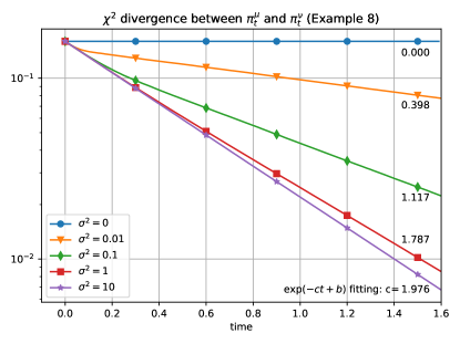
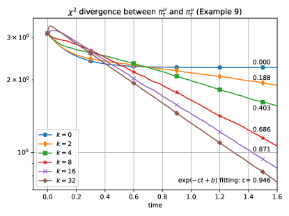
Figure 1: (L) ${\chi^{2}}(\pi_{t}^{\mu}\mid\pi_{t}^{\nu})$ for the model in Example 7.38 with different values of noise intensity $\sigma^{2}$. (R) ${\chi^{2}}(\pi_{t}^{\mu}\mid\pi_{t}^{\nu})$ for the model in Example 7.39 with different values of signal intensity $k$. The number on each line shows the exponential rate obtained from linear fitting.

7.1 Ergodic case

The following is the famous counter-example of the filtering theory that first appeared in [28]. It describes an HMM whose signal is ergodic but the filter is not so.

Example 7.38 (Famous counterexample [28]).

Consider an HMM on $\mathbb{S}=\{1,2,3,4\}$ with generator of the Markov process

$${\cal A}=\begin{pmatrix}-1&1&0&0\\ 0&-1&1&0\\ 0&0&-1&1\\ 1&0&0&-1\end{pmatrix}$$

The Markov process is ergodic with ${\bar{\mu}}=[\frac{1}{4},\frac{1}{4},\frac{1}{4},\frac{1}{4}]^{\hbox{\rm\tiny T}}$ as the invariant measure. The observation model is assumed noiseless as follows:

$$Z_{t}=h(X_{t})\quad\text{where}\quad h=\begin{pmatrix}h(1)\\ h(2)\\ h(3)\\ h(4)\end{pmatrix}=\begin{pmatrix}1\\ 0\\ 1\\ 0\end{pmatrix}$$

The observations provide time instants $\{t_{k}\geq 0:k=1,2,\ldots\}$ when the process jumps from one state to another (possible transitions are $1\mapsto 2$, $2\mapsto 3$, $3\mapsto 4$, and $4\mapsto 1$). For $t_{k}\leq t<t_{k+1}$, $\pi_{t}$ is constant. Table 3 illustrates a sample path of the observation process and the filter. From this analysis, it follows that with two different initializations, $\mu$ with $p=\frac{\mu(1)}{\mu(1)+\mu(3)}$, and $\nu$ with $p^{\prime}=\frac{\nu(1)}{\nu(1)+\nu(3)}$,

$$\|\pi_{t}^{\mu}-\pi_{t}^{\nu}\|_{\text{\tiny TV}}=2(p-p^{\prime}),\quad\forall\,t>0$$

Therefore, the filter is not stable (even though the Markov process is).

Table 3: A sample path of the filter for Example 7.38

$t$	$[0,t_{1})$	$[t_{1},t_{2})$	$[t_{2},t_{3})$	$[t_{3},t_{4})$	$[t_{4},t_{5})$	$\cdots$
$Z_{t}$	1	0	1	0	1	$\cdots$
$\pi_{t}^{\mu}(1)$	$p$	0	$1-p$	0	$p$	$\cdots$
$\pi_{t}^{\mu}(2)$	0	$p$	0	$1-p$	0	$\cdots$
$\pi_{t}^{\mu}(3)$	$1-p$	0	$p$	0	$1-p$	$\cdots$
$\pi_{t}^{\mu}(4)$	0	$1-p$	0	$p$	0	$\cdots$

An explanation in terms of the conditional PI is as follows: For the deterministic observation model, the sigma-algebra generated by the observation ${\cal Z}_{t}=\sigma([X_{t}\in\{1,3\}])$. Consider a ${\cal Z}_{t}$-measurable function:

$$F(\cdot)=\begin{cases}\begin{pmatrix}1&1&-1&-1\end{pmatrix}&\text{if}\;\;X_{t}\in\{1,3\}\\[4.0pt] \begin{pmatrix}-1&1&1&-1\end{pmatrix}&\text{if}\;\;X_{t}\in\{2,4\}\end{cases}$$

Because the nonlinear filter

$$\pi_{t}^{\bar{\mu}}(\cdot)={\sf E}^{\bar{\mu}}({\sf 1}_{[X_{t}=\cdot]}\mid{\cal Z}_{t})=\begin{cases}\begin{pmatrix}\frac{1}{2}&0&\frac{1}{2}&0\end{pmatrix}&\text{if}\;\;X_{t}\in\{1,3\}\\[4.0pt] \begin{pmatrix}0&\frac{1}{2}&0&\frac{1}{2}\end{pmatrix}&\text{if}\;\;X_{t}\in\{2,4\}\end{cases}$$

the conditional mean $\pi_{t}^{\bar{\mu}}(F)=0$ and the conditional variance ${\cal V}_{t}^{\bar{\mu}}(F)=\pi_{t}^{\bar{\mu}}(F^{2})=1$. Meanwhile, the conditional energy $\pi_{t}^{\bar{\mu}}(\Gamma F)=0$. Therefore, the conditional PI does not hold for this example. (Note that the PI is based on duality which is not applicable for the noiseless observation model.)

Let us examine the situation next upon introduction of an arbitrary small amount of noise. That is, consider the model $\,\mathrm{d}Z_{t}=h(X_{t})\,\mathrm{d}t+\sigma\,\mathrm{d}W_{t}$ with $\sigma\neq 0$. Figure 1 (L) depicts the ${\chi^{2}}$-divergence for choices of $\sigma^{2}\in\{0,0.01,0.1,1,10\}$. For each of these plots, $\mu=[0.35,0.35,0.15,0.15]$ and $\nu=[0.25,0.25,0.25,0.25]$. Observe that the rate increases proportionally as a function of $\sigma^{2}$ with $c\uparrow 2$ as $\sigma^{2}\to\infty$. The constant $c=2$ is the Poincaré constant for the Markov process. Although, these results are omitted here, a rate $c>2$ can be achieved with a suitable choice of $h$ (e.g., with $h(3)=-1$).

7.2 Observable case

Example 7.39.

Consider an HMM on $\mathbb{S}=\{1,2,3,4\}$ with

$${\cal A}=\begin{pmatrix}-1&1&0&0\\ 2&-2&0&0\\ 0&0&-1&1\\ 0&0&2&-2\end{pmatrix},\quad h=\begin{pmatrix}k\\ 0\\ -k\\ 0\end{pmatrix}$$

The components $\{1,2\}$ and $\{3,4\}$ do not have any transitions between them. Therefore, the Markov process is not ergodic. For $k\neq 0$, the HMM is observable: the sign of observation contains information that distinguishes $\{1,2\}$ and $\{3,4\}$.

Figure 1 (R) depicts ${\chi^{2}}$-divergence as a function of the parameter $k$. For $k=0$, the HMM is not observable and the ${\chi^{2}}$-divergence does not converge to zero. For non-zero values of $k$, filter stability is obtained with rate increasing proportionally with $k$. For each of these simulations, $\mu=[0.2,0.6,0.1,0.1]$ and $\nu=[0.1,0.1,0.1,0.7]$ are used. An interesting point to note is that for $k=16$ or $k=32$, the divergence exhibits transient growth (See Remark A.40 in Appendix A.3).

8 Conclusions and Discussion

In this paper, we introduced a novel notion of the Poincaré inequality (PI) for the study of nonlinear filter. The first contribution is the use of PI to obtain a formula for the filter stability (Thm. 5.19). Next, the PI is related to the two model properties, namely, the ergodicity of the signal model (Prop. 6.36); and the observability of the HMM (Prop. 6.32).

8.1 Practical significance

There are two manners in which these results are of practical significance. One, our work is important for the analysis and design of algorithms for numerical approximation of the nonlinear filter [36]. Specifically, the error analysis of these algorithms require estimates of the two constants rated to the exponential decay (the Poincaré constant $c$) and the transient growth (constant $\frac{1}{\underline{a}}$ in Thm. 5.19) [37, Prop. 2]. Ours is the first such study which provides a systematic framework to identify and (in future) improve estimates of the two constants.

The second manner of practical significance comes from design of reinforcement learning (RL) algorithms in partially observed settings of the problem. Many of these algorithms are based on windowing the past observation data and using the windowed data as an approximate information state [38, 39, 40]. The Poincaré constant is useful to estimate the length of the window for approximately optimal performance.

8.2 Future work

The next steps are as follows: Obtain a converse of Prop. 6.32, specifically relate PI to the detectability of HMM. Other important task is to obtain bounds on the rates for general state spaces including when (i) $\mathbb{S}$ is countable; (ii) $\mathbb{S}$ is compact; and (iii) $\mathbb{S}=\mathbb{R}^{d}$. Of particular interest are the problems related to Itô diffusion in $\mathbb{S}\subseteq\mathbb{R}^{d}$.

As a final point, it is noted that the definition of backward map (4) is not limited to the HMMs with white noise observations. This suggests that it may be possible to extend duality and the associated filter stability analysis to a more general class of HMMs.

Appendix A Appendix

A.1 Proof of Proposition 1

Suppose $\mu,\nu\in{\cal P}(\mathbb{S})$ and $\mu\ll\nu$. Let $\gamma=\frac{\,\mathrm{d}\mu}{\,\mathrm{d}\nu}$. Then the three forms of $f$-divergence are defined as follows:

(KL divergence) $${\sf D}(\mu\mid\nu):=\int_{\mathbb{S}}\gamma(x)\log(\gamma(x))\,\mathrm{d}\nu(x)$$

($$\chi^{2} {\chi^{2}}(\mu\mid\nu):=\int_{\mathbb{S}}(\gamma(x)-1)^{2}\,\mathrm{d}\nu(x)$$ divergence)

(Total variation) $$\|\mu-\nu\|_{\text{\tiny TV}}:=\int_{\mathbb{S}}{\mathchoice{\genfrac{}{}{}{1}{1}{2}}{\genfrac{}{}{}{2}{1}{2}}{\genfrac{}{}{}{3}{1}{2}}{\genfrac{}{}{}{4}{1}{2}}}|\gamma(x)-1|\,\mathrm{d}\nu(x)$$

For these, the following inequalities are standard (see [41, Lemma 2.5 and 2.7]):

$$2\|\mu-\nu\|_{\text{\tiny TV}}^{2}\leq{\sf D}(\mu\mid\nu)\leq{\chi^{2}}(\mu\mid\nu)$$

The first inequality is called the Pinsker’s inequality. The result follows directly from using these inequalities. For $L^{2}$ stability, observe that for any $f\in C_{b}(\mathbb{S})$,

$$\pi_{T}^{\mu}(f)-\pi_{T}^{\nu}(f)=\pi_{T}^{\nu}(f\gamma_{T})-\pi_{T}^{\nu}(f)\pi_{T}^{\nu}(\gamma_{T})$$

Therefore by Cauchy-Schwarz inequality,

$$|\pi_{T}^{\mu}(f)-\pi_{T}^{\nu}(f)|^{2}\leq\frac{\operatorname{osc}(f)}{4}{\chi^{2}}(\pi_{T}^{\mu}\mid\pi_{T}^{\nu})$$

where $\operatorname{osc}(f)=\sup_{x\in\mathbb{S}}f(x)-\inf_{x\in\mathbb{S}}f(x)$ denotes the oscillation of $f$. Taking ${\sf E}^{\mu}(\cdot)$ on both sides yields the conclusion.

A.2 Rate bounds for HMM on finite state-space

A majority of the known bounds for exponential rate of convergence are for HMMs on finite state-space. For the ergodic signal model, bounds for the stability index $\bar{\gamma}$ (see Rem. 3.4) are tabulated in Table 4 together with references in literature where these bounds have appeared. All of these bounds have also been derived using the approach of this paper. The bounds are given in terms of the conditional Poincaré constant $c$ (see Rem. 5.29) and appear as examples in our prior conference paper [26].

For the non-ergodic signal model, again in finite state-space settings, additional bounds are known as follows [12, Thm. 7]:

$$\mathop{\operatorname{limsup}}_{r\to 0}r^{2}\overline{\gamma} \leq-{\mathchoice{\genfrac{}{}{}{1}{1}{2}}{\genfrac{}{}{}{2}{1}{2}}{\genfrac{}{}{}{3}{1}{2}}{\genfrac{}{}{}{4}{1}{2}}}\sum_{i\in\mathbb{S}}{\bar{\mu}}(i)\min_{j\neq i}|h(i)-h(j)|^{2}$$

$$\mathop{\operatorname{liminf}}_{r\to 0}r^{2}\overline{\gamma} \leq-{\mathchoice{\genfrac{}{}{}{1}{1}{2}}{\genfrac{}{}{}{2}{1}{2}}{\genfrac{}{}{}{3}{1}{2}}{\genfrac{}{}{}{4}{1}{2}}}\sum_{i,j\in\mathbb{S}}{\bar{\mu}}(i)|h(i)-h(j)|^{2}$$

where $r$ is the standard deviation of the measurement noise $W$. Derivation of these latter pair of bounds using the approach of this paper is open.

Table 4: Rate bounds for finite-state HMM^†

#	Bound	Literature ($-\bar{\gamma}$)	Our work ($c$)
(1)	$\min_{{i\neq j}}\sqrt{A(i,j)A(j,i)}$	[12, Thm. 5]	[26, Ex. 4]
		[8, Thm. 4.3]
		[4, Corr. 2.3.2]
(2)	$\sum_{i\in\mathbb{S}}{\bar{\mu}}(i)\min_{j\neq i}A(i,j)$	[8, Thm. 4.2]	[26, Ex. 2]
(3)	$\sum_{j}\min_{i\neq j}A(i,j)$	[13, Ass. 4.3.24]	[26, Ex. 3]
†$\{A(i,j):1\leq i,j\leq d\}$ is the generator (a transition rate matrix) for the state process and ${\bar{\mu}}$ is an invariant measure.

A.3 Calculation of ${\chi^{2}}$-divergence

Suppose $\{\pi_{t}^{\mu}:t\geq 0\}$ and $\{\pi_{t}^{\nu}:t\geq 0\}$ are the solutions of the nonlinear filtering equation (3) starting from prior $\mu$ and $\nu$, respectively. Then

$$\,\mathrm{d}{\chi^{2}}(\pi_{t}^{\mu}\mid\pi_{t}^{\nu})=-(\pi_{t}^{\nu}\big{(}\Gamma\gamma_{t}\big{)}+{\cal V}_{t}^{\mu}(\gamma_{t},h)\cdot{\cal V}_{t}^{\nu}(\gamma_{t},h))\,\mathrm{d}t+C_{t}^{\hbox{\rm\tiny T}}\,\mathrm{d}I_{t}^{\mu}$$ (17)

where $C_{t}=\pi_{t}^{\mu}\big{(}\gamma_{t}(h+\pi_{t}^{\nu}(h)-2\pi_{t}^{\mu}(h))\big{)}$. With $h=c{\sf 1}$, two terms on the right-hand side are zero and the formula (8) is obtained. Before describing the derivation of (17), a remark concerning the direct use of this equation for the purpose of filter stability is included as follows:

Remark A.40.

The term $-\pi_{t}^{\nu}(\Gamma\gamma_{t})$ on the right-hand side of (8) is non-positive. However, the product ${\cal V}_{t}^{\mu}(\gamma_{t},h)\cdot{\cal V}_{t}^{\nu}(\gamma_{t},h)$ is sign-indeterminate. Therefore, the equation has not been useful for the asymptotic analysis of the ${\chi^{2}}$-divergence.

Derivation of (17): Using the equation (3) for the filter

$$\,\mathrm{d}{\chi^{2}}(\pi_{t}^{\mu}\mid\pi_{t}^{\nu})=\,\mathrm{d}\pi_{t}^{\nu}(\gamma_{t}^{2})=C_{t,1}\,\mathrm{d}t+C_{t,2}^{\hbox{\rm\tiny T}}\,\mathrm{d}I_{t}^{\mu}+C_{t,3}^{\hbox{\rm\tiny T}}\,\mathrm{d}I_{t}^{\nu}$$

where the formulae for the three coefficients, obtained through an application of the Itô’s formula, are as follows:

$$C_{t,1} =\pi_{t}^{\nu}\big{(}\Gamma\gamma_{t}\big{)}+\pi_{t}^{\mu}\big{(}\gamma_{t}|h-\pi_{t}^{\mu}(h)|^{2}\big{)}+\pi_{t}^{\mu}\big{(}\gamma_{t}|h-\pi_{t}^{\nu}(h)|^{2}\big{)}$$

$$\qquad-2\>\pi_{t}^{\mu}\big{(}\gamma_{t}(h-\pi_{t}^{\mu}(h))^{\hbox{\rm\tiny T}}(h-\pi_{t}^{\nu}(h))\big{)}$$

$$C_{t,2} =2\>\pi_{t}^{\mu}\big{(}\gamma_{t}(h-\pi_{t}^{\mu}(h))\big{)},\;\;C_{t,3}=-\pi_{t}^{\nu}\big{(}\gamma_{t}^{2}(h-\pi_{t}^{\nu}(h))\big{)}$$

Upon noting $\,\mathrm{d}I_{t}^{\nu}=\,\mathrm{d}I_{t}^{\mu}+(\pi_{t}^{\mu}(h)-\pi_{t}^{\nu}(h))\,\mathrm{d}t$ and simplifying the formula (17) for divergence is obtained.

A.4 Proof of Theorem 4.11

The feedback control formula (10) is from [2, Thm. 3]. The equation for the conditional mean and variance is proved in [2, Prop. 1]. The SDE (11) for the conditional variance is derived using the Hamilton’s equation arising from the maximum principle of optimal control [2, Thm. 2]. Specifically, for the optimal control problem (9), the co-state process (momentum) is a measure-valued process denoted as $\{P_{t}:0\leq t\leq T\}$. The Hamilton’s equation for momentum is as follows: For $f\in{\cal Y}$,

$$\,\mathrm{d}P_{t}(f)= \big{(}P_{t}({\cal A}f)+2\sigma_{t}^{\rho}(\Gamma(f,Y_{t}))\big{)}\,\mathrm{d}t$$

$$+\big{(}P_{t}(hf)+2U_{t}^{\text{\rm(opt)}}\sigma_{t}^{\rho}(f)+2\sigma_{t}^{\rho}(V_{t}f)\big{)}^{\hbox{\rm\tiny T}}\,\mathrm{d}Z_{t}$$

where $\sigma_{t}^{\rho}$ denotes the unnormalized filter at time $t$ (solution of the DMZ equation starting from initialization $\sigma_{0}^{\rho}=\rho$). From [2, Rem. 5], ${\cal V}_{t}^{\rho}(f,Y_{t})=\dfrac{P_{t}(f)}{2\sigma_{t}^{\rho}({\sf 1})}$. The SDE (11) is then obtained by using the Itô formula.

An alternate derivation of (11) is based on directly using the nonlinear filter (3) to show that

$$\,\mathrm{d}{\cal V}_{t}^{\rho} (f,g)=\Big{(}\pi_{t}^{\rho}\big{(}\Gamma(f,g)\big{)}+{\cal V}_{t}^{\rho}(g,{\cal A}f)$$

$$\qquad+{\cal V}_{t}^{\rho}(f,{\cal A}g)-{\cal V}_{t}^{\rho}(h,f){\cal V}_{t}^{\rho}(h,g)\Big{)}\,\mathrm{d}t$$

$$+\Big{(}{\cal V}_{t}^{\rho}(h,fg)-\pi_{t}^{\rho}(f){\cal V}_{t}^{\rho}(h,g)-\pi_{t}^{\rho}(g){\cal V}_{t}^{\rho}(h,f)\Big{)}^{\hbox{\rm\tiny T}}\,\mathrm{d}I_{t}^{\rho}$$

With $g=Y_{t}$, using the BSDE (9b) with $U_{t}=U_{t}^{\text{\rm(opt)}}$, upon simplifying, again yields (11).

A.5 Proof of Lemma 5.16

For $F\in\mathbb{H}_{\tau}^{\rho}$, we begin by noting

$$\|F\|_{\mathbb{H}_{\tau}^{\rho}}^{2}={\tilde{\sf E}}^{\rho}\big{(}\sigma_{\tau}^{\rho}(F^{2})\big{)}={\sf E}^{\rho}\big{(}\pi_{\tau}^{\rho}(F^{2})\big{)}={\sf E}^{\rho}\big{(}(F(X_{\tau}))^{2}\big{)}$$ (18)

We are interested in minimizers of the energy functional ${\cal E}(F)$ for $F\in\mathbb{H}_{\tau}^{\rho}$. The minimizer is not unique because of the following translation symmetry:

$${\cal E}(F+\alpha{\sf 1})={\cal E}(F)$$

for any ${\cal Z}_{\tau}$-measurable random variable $\alpha$ such that ${\tilde{\sf E}}^{\rho}(\alpha^{2})<\infty$. For this reason, consider the subspace

$${\cal S}:=\{F\in\mathbb{H}_{\tau}^{\rho}\;:\;\pi_{\tau}^{\rho}(F)=0,\;\;{\sf P}^{\rho}-a.s.\}$$

Then $\cal S$ is closed subspace. (Suppose $F^{(n)}\to F$ in $\mathbb{H}_{\tau}^{\rho}$ with $\pi^{\rho}_{\tau}\big{(}F^{(n)}\big{)}=0$. Then ${\sf E}^{\rho}\big{(}|\pi^{\rho}_{\tau}(F)|\big{)}={\sf E}^{\rho}\big{(}|\pi^{\rho}_{\tau}(F-F^{(n)})|\big{)}\leq{\sf E}^{\rho}\big{(}\pi^{\rho}_{\tau}(|F-F^{(n)}|^{2})\big{)}={\tilde{\sf E}}^{\rho}\big{(}\sigma_{\tau}^{\rho}(|F-F^{(n)}|^{2})\big{)}\to 0$.).

Proposition A.41.

Consider the optimal control problem (9) with $F\in{\cal S}$. Then

1. The optimal control $U^{\text{\rm(opt)}}=0$.

2. At time $t=0$, $\rho(Y_{0})=0$.

Proof A.42.

See Appendix A.7.

For optimal control system (12), define the solution operator

$${\sf L}^{\rho}:\mathbb{H}_{\tau}^{\rho}\to\mathbb{H}^{\rho}([0,\tau])\times\mathbb{H}^{\rho}([0,\tau])^{m}\quad\text{by}\quad{\sf L}^{\rho}(F):=(Y,V)$$

Recall that we have already defined the operator ${\sf L}^{\rho}_{0}:\mathbb{H}_{\tau}^{\rho}\to L^{2}(\rho)$ such that ${\sf L}^{\rho}_{0}(F)=Y_{0}$.

Because $U^{\text{\rm(opt)}}=0$, with $(Y,V)={\sf L}^{\rho}(F)$, the formula for energy becomes

$${\cal E}^{\rho}(F)=\frac{1}{\tau}{\sf E}^{\rho}\left(\int_{0}^{\tau}\pi_{t}^{\rho}(\Gamma Y_{t})+\pi_{t}^{\rho}(|V_{t}|^{2})\,\mathrm{d}t\right),\quad F\in{\cal S}$$

where note $\pi_{t}^{\rho}(|V_{t}|^{2}):=\int_{\mathbb{S}}V_{t}^{\hbox{\rm\tiny T}}(x)V_{t}(x)\,\mathrm{d}\pi_{t}^{\rho}(x)$. The optimality equation (11b) gives

$$\rho(Y_{0}^{2})+\tau{\cal E}(F)={\sf E}^{\rho}((F(X_{\tau}))^{2}),\quad F\in{\cal S}$$ (19)

This shows that ${\sf L}^{\rho}_{0}:{\cal S}\to L^{2}(\rho)$ is a bounded operator with $\|{\sf L}^{\rho}_{0}\|\leq 1$. Because $\rho(Y_{0})=0$,

$$c^{\rho}=\inf\{{\cal E}^{\rho}(F)\;:\;F\in{\cal S},\;Y_{0}={\sf L}^{\rho}_{0}(F)\;\;\&\;\;\rho(Y_{0}^{2})=1\}$$

To obtain the minimizer, setting $(\tilde{Y},\tilde{V})={\sf L}^{\rho}(\tilde{F})$ for $\tilde{F}\in{\cal S}$, the functional derivative is computed as follows:

$$\langle\nabla{\cal E}^{\rho}(F),\tilde{F}\rangle:=\frac{2}{\tau}{\sf E}^{\rho}\left(\int_{0}^{\tau}\pi_{t}^{\rho}(\Gamma(Y_{t},\tilde{Y}_{t})+\pi_{t}^{\rho}(V_{t}^{\hbox{\rm\tiny T}}\tilde{V}_{t})\,\mathrm{d}t\right)$$

where note $\pi_{t}^{\rho}(V_{t}^{\hbox{\rm\tiny T}}\tilde{V}_{t}):=\int_{\mathbb{S}}V_{t}^{\hbox{\rm\tiny T}}(x)\tilde{V}_{t}(x)\,\mathrm{d}\pi_{t}^{\rho}(x)$. From the Cauchy-Schwarz formula, using (18) and (19),

$$|\langle\nabla{\cal E}^{\rho}(F),\tilde{F}\rangle|^{2}\leq\frac{4}{\tau^{2}}\|F\|_{\mathbb{H}_{\tau}^{\rho}}^{2}\;\|\tilde{F}\|_{\mathbb{H}_{\tau}^{\rho}}^{2}$$ (20)

This shows that $\tilde{F}\mapsto\langle\nabla{\cal E}^{\rho}(F),\tilde{F}\rangle$ is a bounded linear functional as a map from $\tilde{F}\in\mathbb{H}_{\tau}^{\rho}$ into $\mathbb{R}$. With these formalities completed, we provide a proof of Lemma 5.16.

Proof A.43 (of Lemma 5.16).

Consider an infimizing sequence $\{F^{(n)}\in{\cal S}:n=1,2,\ldots\}$ such that ${\cal E}^{\rho}\big{(}F^{(n)}\big{)}\to c^{\rho}$ and $\rho\big{(}(Y_{0}^{(n)})^{2}\big{)}=1$ with $Y_{0}^{(n)}:={\sf L}^{\rho}_{0}\big{(}F^{(n)}\big{)}$. The proof is obtained in three steps:

Step 1: Establish a limit $F\in\mathbb{H}_{\tau}^{\rho}$ such that $F^{(n)}$ converges weakly (in $\mathbb{H}_{\tau}^{\rho}$) to $F$. The weak convergence is denoted as $F^{(n)}\rightharpoonup F$.

Step 2: Show that ${\cal E}^{\rho}(F)=c^{\rho}$.

Step 3:. Set $Y_{0}={\sf L}^{\rho}_{0}(F)$. Show that $\rho(Y_{0})=0$, $\rho(Y_{0}^{2})=1$.

To establish a limit, use the optimality equation (19):

$$\rho\big{(}(Y_{0}^{(n)})^{2}\big{)}+\tau{\cal E}(F^{(n)})={\sf E}^{\rho}\big{(}(F^{(n)}(X_{\tau}))^{2}\big{)},\quad n=1,2,\ldots$$

Now $\rho\big{(}(Y_{0}^{(n)})^{2}\big{)}=1$ and because ${\cal E}(F^{(n)})\to c^{\rho}$, by considering a sub-sequence if necessary, using (18),

$$\|F^{(n)}\|_{\mathbb{H}_{\tau}^{\rho}}^{2}={\sf E}^{\rho}((F^{(n)}(X_{\tau}))^{2})<1+\tau(c^{\rho}+1)$$

We thus have a bounded sequence in the Hilbert space $\mathbb{H}_{\tau}^{\rho}$. Therefore, there exists a weak limit $F\in\mathbb{H}_{\tau}^{\rho}$ such that $F^{(n)}\rightharpoonup F$. This completes the proof of Step 1.

Next we show ${\cal E}^{\rho}(F)=c^{\rho}$. Because the map from $F\mapsto{\cal E}^{\rho}(F)$ is convex, we have

$${\cal E}^{\rho}(F^{(n)})\geq{\cal E}^{\rho}(F)+\langle\nabla{\cal E}^{\rho}(F),(F^{(n)}-F)\rangle$$

We have already shown that $\tilde{F}\mapsto\langle\nabla{\cal E}^{\rho}(F),\tilde{F}\rangle$ is a bounded linear functional. Therefore, letting $n\to\infty$, the second term on the right-hand side converges to zero and

$$\mathop{\operatorname{liminf}}_{n\to\infty}{\cal E}^{\rho}(F^{(n)})\geq{\cal E}^{\rho}(F)$$

This property of the functional is referred to as weak lower semi-continuity. Because ${\cal E}^{\rho}(F^{(n)})\to c^{\rho}$, we have ${\cal E}^{\rho}(F)\leq c^{\rho}$. However, $c^{\rho}$ is the infimum. It therefore must be that ${\cal E}^{\rho}(F)=c^{\rho}$. This completes the proof of the Step 2.

The step 3 of the proof is to show that setting $Y_{0}:={\sf L}^{\rho}_{0}(F)$ gives $\rho(Y_{0})=0$ and $\rho(Y_{0}^{2})=1$. This is where the assumption on compactness of ${\sf L}^{\rho}_{0}$ is used. Because $F^{(n)}\rightharpoonup F$ in $\mathbb{H}_{\tau}^{\rho}$ and ${\sf L}^{\rho}_{0}$ is compact, we have $Y_{0}^{(n)}\to Y_{0}$ in $L^{2}(\rho)$. Then $|\rho(Y_{0})|=|\rho(Y_{0}-Y_{0}^{(n)})|\leq\rho\big{(}|Y_{0}-Y_{0}^{(n)}|^{2}\big{)}\to 0$ and $\rho(Y_{0}^{2})=\lim_{n\to\infty}\rho\big{(}(Y_{0}^{(n)})^{2}\big{)}=1$ by the continuity of the norm with respect to strong convergence.

A.6 Lower bound for the ratio $R_{T}$

Proof of $R_{t}\geq\underline{a}$: Since $R_{T}$ is the ratio of expectations of the same random variable ${\cal V}_{T}^{\nu}(\gamma_{T})={\chi^{2}}(\pi_{T}^{\mu}|\pi_{T}^{\nu})$ under measures ${\sf P}^{\mu}$ and ${\sf P}^{\nu}$

$$R_{T}=\frac{{\sf E}^{\mu}\big{(}{\cal V}^{\nu}_{T}(\gamma_{T})\big{)}}{{\sf E}^{\nu}\big{(}{\cal V}^{\nu}_{T}(\gamma_{T})\big{)}}\geq\mathop{\operatorname{essinf}}_{\omega\in\Omega}\frac{\,\mathrm{d}{\sf P}^{\mu}}{\,\mathrm{d}{\sf P}^{\nu}}(\omega)=\mathop{\operatorname{essinf}}_{x\in\mathbb{S}}\frac{\,\mathrm{d}\mu}{\,\mathrm{d}\nu}(x)=\underline{a}$$

Remark A.44 (Lower bound for the ratio $R_{T}$).

An alternative formula for the ratio is as follows:

$$R_{T}=\frac{{\sf E}^{\mu}\big{(}{\cal V}_{T}^{\nu}(\gamma_{T})\big{)}}{{\sf E}^{\nu}\big{(}{\cal V}_{T}^{\nu}(\gamma_{T})\big{)}}=\frac{{\sf E}^{\nu}\big{(}A_{T}{\cal V}_{T}^{\nu}(\gamma_{T})\big{)}}{{\sf E}^{\nu}\big{(}{\cal V}_{T}^{\nu}(\gamma_{T})\big{)}}$$

where the change of measure (see [9, Sec. 4.5.1]):

$$\quad A_{T}:=\frac{\,\mathrm{d}{\sf P}^{\mu}|_{{\cal Z}_{T}}}{\,\mathrm{d}{\sf P}^{\nu}|_{{\cal Z}_{T}}}=\exp\Big{(} \int_{0}^{T}(\pi_{t}^{\mu}(h)-\pi_{t}^{\nu}(h))\,\mathrm{d}I^{\mu}_{t}$$

$$-{\mathchoice{\genfrac{}{}{}{1}{1}{2}}{\genfrac{}{}{}{2}{1}{2}}{\genfrac{}{}{}{3}{1}{2}}{\genfrac{}{}{}{4}{1}{2}}}\int_{0}^{T}|\pi_{t}^{\mu}(h)-\pi_{t}^{\nu}(h)|^{2}\,\mathrm{d}t\Big{)}$$

Now, $\{A_{T}:T\geq 0\}$ is a non-negative ${\sf P}^{\nu}$-martingale with ${\sf E}^{\nu}(A_{T})={\sf E}^{\nu}(A_{0})=1$ and therefore, by the martingale convergence theorem, there exists a random variable $A_{\infty}$ such that $A_{T}\stackrel{{\scriptstyle(T\to\infty)}}{{\longrightarrow}}A_{\infty}$. It is possible that an improved asymptotic lower bound for $R_{T}$ can be obtained by showing that $\text{essinf}_{\omega\in\Omega}A_{\infty}(\omega)>0$.

A.7 Proof of Prop. 5.21 and Prop. A.41

Suppose $\pi_{\tau}^{\rho}(F)=c$ where $c$ is a deterministic constant. Using (11a), because ${\tilde{\sf P}}^{\rho}\sim{\sf P}^{\rho}$,

$$c=\rho(Y_{0})-\int_{0}^{\tau}\big{(}U_{t}^{\text{\rm(opt)}}\big{)}^{\hbox{\rm\tiny T}}\,\mathrm{d}Z_{t},\quad{\tilde{\sf P}}^{\rho}\text{-a.s.}$$

By the uniqueness of the Itô representation, then

$$U_{t}^{\text{\rm(opt)}}=0,\quad\text{a.e.}\;0\leq t\leq\tau,\;\;{\tilde{\sf P}}^{\rho}\text{-a.s.}$$

and, because these are equivalent, also ${\sf P}^{\rho}\text{-a.s.}$. Using (11a), this also gives

$$\pi_{t}^{\rho}(Y_{t})=c,\quad{\sf P}^{\rho}\text{-a.s.}\;\;\text{a.e.}\;0\leq t\leq\tau$$

and ${\sf E}^{\rho}\big{(}{\cal V}_{t}^{\rho}(Y_{t})\big{)}={\sf E}^{\rho}(|Y_{t}(X_{t})-c|^{2})=\text{var}^{\rho}\big{(}Y_{t}(X_{t})\big{)}$.

Now consider the stochastic process $\{Y_{t}(X_{t}):0\leq t\leq\tau\}$. Because $U=0$, the Itô-Wentzell formula is used to show that (see [1, Appdx. A])

$$\,\mathrm{d}Y_{t}(X_{t})=V_{t}^{\hbox{\rm\tiny T}}(X_{t})\,\mathrm{d}W_{t}+\,\mathrm{d}N_{t},\quad 0\leq t\leq\tau$$

where $\{N_{t}:t\geq 0\}$ is a ${\sf P}^{\rho}$-martingale. Integrating this from $t$ to $\tau$ yields

$$F(X_{\tau})=Y_{t}(X_{t})+\int_{t}^{\tau}V_{s}^{\hbox{\rm\tiny T}}(X_{s})\,\mathrm{d}W_{s}+\,\mathrm{d}N_{s}$$

which gives

$$Y_{t}(x)={\sf E}^{\rho}\big{(}F(X_{T})\mid{\cal Z}_{t}\vee[X_{t}=x]\big{)},\;\;x\in\mathbb{S},\;\;{\sf P}^{\rho}\text{-a.s.}$$

Proof A.45 (of Prop. 5.21).

Set $\rho=\nu$ and $\tau=T$. If $F\in{\cal L}_{T}^{\nu}$ the representation as a conditional expectation shows $Y_{t}(x)\geq 0$, and because $\pi_{t}^{\nu}(Y_{t})=1$, $Y_{t}$ is a likelihood ratio. For $F=\gamma_{T}$,

$$Y_{0}(x)={\sf E}^{\nu}(\gamma_{T}(X_{T})|[X_{0}=x]),\quad x\in\mathbb{S}$$

The righthand-side is the backward map (4) which proves $Y_{0}(x)=y_{0}(x)$.

A.8 Derivation of the uniform bound (15)

In this paper, we have derived two formulae for the $\chi^{2}$-divergence between $\pi_{T}^{\mu}$ and $\pi_{T}^{\nu}$, with respect to the probability measures ${\sf P}^{\nu}$ and ${\sf P}^{\mu}$. These formulae are as follows:

1. Noting

   $$\text{var}^{\nu}(\gamma_{T}(X_{T}))={\sf E}^{\nu}(\pi_{T}^{\nu}(\gamma_{T}^{2})-1)={\sf E}^{\nu}(\chi^{2}(\pi_{T}^{\mu}|\pi_{T}^{\nu}))$$

   the formula with respect to ${\sf P}^{\nu}$ is given by (14),

   $${\sf E}^{\nu}(\chi^{2}(\pi_{T}^{\mu}|\pi_{T}^{\nu}))$$

   $$=\text{var}^{\nu}(Y_{0}(X_{0}))+\int_{0}^{T}{\sf E}^{\nu}\left(\pi_{t}^{\nu}(\Gamma Y_{t})+\pi_{t}^{\nu}(|V_{t}|^{2})\right)\,\mathrm{d}t$$

2. The second formula, with respect to ${\sf P}^{\mu}$, is given by (5) repeated here using the notation $Y_{0}$ instead of $y_{0}$,

   $$|{\sf E}^{\mu}(\chi^{2}(\pi_{T}^{\mu}|\pi_{T}^{\nu}))|^{2}\leq\text{var}^{\nu}(Y_{0}(X_{0}))\text{var}^{\nu}(\gamma_{0}(X_{0}))$$

Combining the two formulae

$$\text{var}^{\nu}(Y_{0}(X_{0}))+\int_{0}^{T}{\sf E}^{\nu}\left(\pi_{t}^{\nu}(\Gamma Y_{t})+\pi_{t}^{\nu}(|V_{t}|^{2})\right)\,\mathrm{d}t$$

$$=\frac{1}{R_{T}}{\sf E}^{\mu}(\pi_{T}^{\nu}(\gamma_{T}^{2})-1)\leq\frac{1}{R_{T}}\left(\text{var}^{\nu}(Y_{0}(X_{0}))\text{var}^{\nu}(\gamma_{0}(X_{0}))\right)^{\mathchoice{\genfrac{}{}{}{1}{1}{2}}{\genfrac{}{}{}{2}{1}{2}}{\genfrac{}{}{}{3}{1}{2}}{\genfrac{}{}{}{4}{1}{2}}}$$

where

$$R_{T}:=\frac{{\sf E}^{\mu}(\chi^{2}(\pi_{T}^{\mu}|\pi_{T}^{\nu}))}{{\sf E}^{\nu}(\chi^{2}(\pi_{T}^{\mu}|\pi_{T}^{\nu}))}$$

We therefore arrive at two apriori bounds:

$$R_{T}^{2}\text{var}^{\nu}(Y_{0}(X_{0}))\leq\text{var}^{\nu}(\gamma_{0}(X_{0}))$$

$$R_{T}^{2}\int_{0}^{T}{\sf E}^{\nu}\left(\pi_{t}^{\nu}(\Gamma Y_{t})+\pi_{t}^{\nu}(|V_{t}|^{2})\right)\,\mathrm{d}t\leq\text{var}^{\nu}(\gamma_{0}(X_{0}))$$

The uniform bound (15) follows because $R_{T}\geq\underline{a}$.

A.9 Proof of Lemma 5.24

The proof requires showing a Markov property of the optimal control system (12).

Markov property of the optimal control system: Because $U^{\text{\rm(opt)}}=0$, the optimal control system (12) is the BSDE

$$-\,\mathrm{d}Y_{t}(x) =\big{(}({\cal A}Y_{t})(x)+h^{\hbox{\rm\tiny T}}(x)V_{t}(x)\big{)}\,\mathrm{d}t-V_{t}^{\hbox{\rm\tiny T}}(x)\,\mathrm{d}Z_{t},$$

$$\quad Y_{T}(x) =\gamma_{T}(x)=\frac{\,\mathrm{d}\pi_{T}^{\mu}}{\,\mathrm{d}\pi_{T}^{\nu}}(x),\;\;x\in\mathbb{S},\;\;0\leq t\leq T$$ (21)

Since the terminal value $Y_{T}$ is a function of $\pi_{T}^{\nu}$ and $\pi_{T}^{\mu}$, which are both Markov processes, the Markov property follows from the theory of forward-backward SDEs [42, Chapter 5]. Specifically, for time $s\in[t,T]$, let $\pi_{s}^{p,t}$ denote the solution of (3) with initial condition $\pi_{t}=p$. Then

$$\pi_{s}^{\pi_{t}^{\mu}(\omega),t}(\omega)=\pi_{s}^{\mu}(\omega),\;\;{\sf P}^{\mu}\text{-a.e.}\;\omega,\;\;t\leq s\leq T$$

$$\pi_{s}^{\pi_{t}^{\nu}(\omega),t}(\omega)=\pi_{s}^{\nu}(\omega),\;\;{\sf P}^{\nu}\text{-a.e.}\;\omega,\;\;t\leq s\leq T$$

Therefore, express

$$\gamma_{T}(x)=\frac{\,\mathrm{d}\pi_{T}^{\mu}}{\,\mathrm{d}\pi_{T}^{\nu}}(x)=\frac{\,\mathrm{d}\pi_{T}^{\pi_{t}^{\mu},t}}{\,\mathrm{d}\pi_{T}^{\pi_{t}^{\nu},t}}(x),\;\;x\in\mathbb{S}$$

and consider the following BSDE over the time-horizon $[t,T]$:

$$-\,\mathrm{d}\tilde{Y}_{s}(x) =\big{(}({\cal A}\tilde{Y}_{s})(x)+h^{\hbox{\rm\tiny T}}(x)\tilde{V}_{s}(x)\big{)}\,\mathrm{d}s-\tilde{V}_{s}^{\hbox{\rm\tiny T}}(x)\,\mathrm{d}Z_{s},$$

$$\quad\tilde{Y}_{T}(x) =\frac{\,\mathrm{d}\pi_{T}^{\pi_{t}^{\mu},t}}{\,\mathrm{d}\pi_{T}^{\pi_{t}^{\nu},t}}(x),\;\;x\in\mathbb{S},\;\;t\leq s\leq T$$

Note that the solution $(\tilde{Y},\tilde{V})=\{(\tilde{Y}_{s},\tilde{V}_{s}):t\leq s\leq T\}$ depends on $\pi_{t}^{\nu}$ and $\pi_{t}^{\mu}$ because of the nature of the terminal condition. The theory of Markov BSDE is used to assert the following (see [42, Ch. 5]):

Lemma A.46 (Markov property of the BSDE).

Let $(Y,V)=\{(Y_{t},V_{t}):0\leq t\leq T\}$ be the solution of (21). Then

• $\tilde{Y}_{s}=Y_{s}$ and $\tilde{V}_{s}=V_{s}$ for all $t\leq s\leq T$, ${\sf P}^{\nu}$-a.s..

• Given $\pi_{t}^{\mu}$ and $\pi_{t}^{\nu}$ at time $t$, $\{(\tilde{Y}_{s},\tilde{V}_{s}):t\leq s\leq T\}$ is independent of ${\cal Z}_{t}$.

Proof A.47.

See [42, Thm. 5.1.3].

Remark A.48.

A corollary to the Markov property is the following representation of the solution

$$Y_{t}=\phi_{t}(\pi_{t}^{\nu},\pi_{t}^{\mu}),\quad 0\leq t\leq T$$

where $\phi_{t}(\cdot,\cdot)$ is a deterministic function of its arguments. While interesting, the representation is not used in this paper.

Proof A.49 (Proof of Lemma 5.24).

Based on the Markov property, the following transformation holds ${\sf P}^{\nu}$-a.s.:

$${\sf E}^{\nu}\Big{(} \int_{t}^{t+\tau}(\Gamma Y_{s})(X_{s})+|V_{s}(X_{s})|^{2}\,\mathrm{d}s\,\big{|}\,{\cal Z}_{t}\Big{)}$$

$$={\sf E}^{\nu}\Big{(}\int_{t}^{t+\tau}\pi_{s}^{\pi_{t}^{\nu},t}\big{(}\Gamma\tilde{Y}_{s}\big{)}+\pi_{s}^{\pi_{t}^{\nu},t}\big{(}|\tilde{V}_{s}|^{2}\big{)}\,\mathrm{d}s\,\big{|}\,{\cal Z}_{t}\Big{)}$$

$$={\sf E}^{\pi_{t}^{\nu}}\Big{(}\int_{0}^{\tau}\pi_{t+s}^{\pi_{t}^{\nu},t}\big{(}\Gamma\tilde{Y}_{t+s}\big{)}+\pi_{t+s}^{\pi_{t}^{\nu},t}\big{(}|\tilde{V}_{t+s}|^{2}\big{)}\,\mathrm{d}s\Big{)}$$

Upon taking an expectation,

$$\frac{1}{\tau}{\sf E}^{\nu}\Big{(}\int_{t}^{t+\tau}\pi_{t}^{\nu}(\Gamma Y_{s})+\pi_{t}^{\nu}(|V_{s}|^{2})\,\mathrm{d}s\Big{)}$$

$$\quad=\frac{1}{\tau}{\sf E}^{\nu}\left({\sf E}^{\pi_{t}^{\nu}}\Big{(}\int_{0}^{\tau}\pi_{t+s}^{\pi_{t}^{\nu},t}\big{(}\Gamma\tilde{Y}_{t+s}\big{)}+\pi_{t+s}^{\pi_{t}^{\nu},t}\big{(}\big{|}\tilde{V}_{t+s}\big{|}^{2}\big{)}\,\mathrm{d}s\Big{)}\right)$$

$$\quad\stackrel{{\scriptstyle\text{(PI)}}}{{\geq}}{\sf E}^{\nu}\left(c^{\pi_{t}^{\nu}}\pi_{t}^{\nu}(\tilde{Y}_{t}^{2}-1)\right)={\sf E}^{\nu}\left(c^{\pi_{t}^{\nu}}{\cal V}_{t}^{\nu}(Y_{t})\right)\;\;(\because,\;Y_{t}=\tilde{Y}_{t})$$

where $c^{\pi_{t}^{\nu}}$ is now a random number given by the Poincaré constant for $\rho=\pi_{t}^{\nu}$.

A.10 Proof of Prop. 6.32 (observable case)

The key to prove the result is the following Lemma:

Lemma A.50.

Suppose ${\cal E}^{\rho}(F)=0$. Then for each $f\in{\cal O}$,

$${\cal V}_{t}^{\rho}(f,Y_{t})=0,\quad{\sf P}^{\rho}\text{-a.s.},\;\;\text{a.e.}\;0\leq t\leq\tau$$

Proof A.51.

From the defining relation for ${\cal E}^{\rho}(F)$,

$$\pi_{t}^{\rho}(\Gamma Y_{t})=0,\;{\cal V}_{t}^{\rho}(h,Y_{t})=0,\;{\cal V}_{t}^{\rho}(V_{t})=0,\;\;{\sf P}^{\rho}\text{-a.s.}$$

for $\text{a.e.}\;0\leq t\leq\tau$. Using the Cauchy-Schwarz formula then for each $f\in C_{b}(\mathbb{S})$,

$$|{\cal V}_{t}^{\rho}(f,V_{t})|^{2}\leq{\cal V}_{t}^{\rho}(f){\cal V}_{t}^{\rho}(V_{t})=0\quad{\sf P}^{\rho}\text{-a.s.}$$

Similarly, upon using the Cauchy-Schwarz formula [31, Eq.1.4.3] for the carré du champ operator,

$$\pi_{t}^{\rho}(\Gamma(f,Y_{t}))=0,\quad{\sf P}^{\rho}\text{-a.s.}$$

Based on these, the SDE (11) for the conditional covariance simplifies to

$$\,\mathrm{d}{\cal V}_{t}^{\rho}(f,Y_{t})={\cal V}_{t}^{\rho}({\cal A}f,Y_{t})\,\mathrm{d}t$$

$$\quad+\big{(}{\cal V}_{t}^{\rho}(hf,Y_{t})-\pi_{t}^{\rho}(h){\cal V}_{t}^{\rho}(f,Y_{t})\big{)}^{\hbox{\rm\tiny T}}\,\mathrm{d}I_{t}^{\rho},\quad 0\leq t\leq\tau$$

Therefore,

$${\cal V}_{t}^{\rho}(f,Y_{t})=0,\;\;\;0\leq t\leq\tau$$

$$\Longrightarrow\quad{\cal V}_{t}^{\rho}({\cal A}f,Y_{t})=0,\;{\cal V}_{t}^{\rho}(hf,Y_{t})=0,\;\;\;0\leq t\leq\tau$$

Since ${\cal V}_{t}^{\rho}({\sf 1},Y_{t})=0$ for all $t\in[0,\tau]$, the result follows from Defn. 6.30 of the observable space ${\cal O}$.

Based on the result in Lemma A.50, the proof of Prop. 6.32 is completed as follows:

Proof A.52 (Proof of Prop. 6.32 (observable case)).

Because $Y_{0}={\sf L}^{\rho}_{0}(F)$ and ${\sf L}^{\rho}_{0}$ is bounded, $Y_{0}\in L^{2}(\rho)$. If $\mathbb{S}$ is finite there is nothing to prove because ${\cal O}=\mathbb{R}^{d}$. In the case where ${\cal O}\subsetneq\bar{{\cal O}}=L^{2}(\rho)$, there exists a sequence $\{f_{n}\in{\cal O}:n=1,2,\ldots\}$ such that $f_{n}\to Y_{0}$ in $L^{2}(\rho)$. From Lemma A.50, for each $n$,

$${\cal V}_{0}^{\rho}(f_{n},Y_{0})=0,\quad{\sf P}^{\rho}\text{-a.s.}$$

Therefore,

$$\text{var}^{\rho}(Y_{0}(X_{0})={\cal V}_{0}^{\rho}(Y_{0}) ={\cal V}_{0}^{\rho}(Y_{0}-f_{n},Y_{0})$$ (22)

and letting $n\to\infty$, because $f_{n}\to Y_{0}$, $\text{var}^{\rho}(Y_{0}(X_{0}))=0$ using the Cauchy-Schwarz.

A.11 Proof of Prop. 6.36 (ergodic case)

At time $t$, let $\rho_{t}$ denote the probability law of $X_{t}$ (without conditioning). Then because the Markov process is ergodic, for any $t>0$, the invariant measure ${\bar{\mu}}\ll\rho_{t}$ (as measures on $\mathbb{S}$). W.l.o.g., take $\mathbb{S}^{\prime}=\text{supp}(\rho_{t})$ as the new state-space and consider the Markov process on $\mathbb{S}^{\prime}$. It is again ergodic with the invariant measure ${\bar{\mu}}\in{\cal P}(\mathbb{S}^{\prime})$ and using Defn. 6.34 of ergodicity,

$$\Gamma f(x)=0,\;\;\forall x\in\mathbb{S}^{\prime}\implies f(x)=c,\;\;\forall x\in\mathbb{S}^{\prime}$$ (23)

Suppose ${\cal E}^{\rho}(F)=0$. Because ${\sf P}^{\rho}\sim{\tilde{\sf P}}^{\rho}$,

$${\sf E}^{\rho}\left(\int_{0}^{\tau}\Gamma Y_{t}(X_{t})\,\mathrm{d}t\right) =0$$

$$\implies\Gamma Y_{t}(X_{t}) =0,\;\;{\tilde{\sf P}}^{\rho}\text{-a.s.},\;\text{a.e.}\;0\leq t\leq\tau$$

Pick a positive $t$ such that $\Gamma Y_{t}(X_{t})=0$, ${\tilde{\sf P}}^{\rho}\text{-a.s.}$. Now, under ${\tilde{\sf P}}^{\rho}$, $X_{t}\sim\rho_{t}$, and $X_{t}$ and $Y_{t}$ are independent. Therefore,

$$0={\tilde{\sf E}}^{\rho}(\Gamma Y_{t}(X_{t}))={\tilde{\sf E}}^{\rho}(\rho_{t}(\Gamma Y_{t}))\implies\rho_{t}(\Gamma Y_{t})=0,\;\;{\tilde{\sf P}}^{\rho}\text{-a.s.}$$

Using (23),

$$\rho_{t}(\Gamma Y_{t})=0,\;\;{\tilde{\sf P}}^{\rho}\text{-a.s.}\implies Y_{t}(x)=c_{t},\;\;x\in\mathbb{S}^{\prime},\;{\tilde{\sf P}}^{\rho}\text{-a.s.}$$

where $c_{t}$ is ${\cal Z}_{t}$-measurable. Then because ${\sf P}^{\rho}\sim{\tilde{\sf P}}^{\rho}$,

$${\sf E}^{\rho}({\cal V}_{t}^{\rho}(Y_{t}))\leq{\sf E}^{\rho}(|Y_{t}(X_{t})-c_{t}|^{2})=0$$

and the result follows because $\text{var}^{\rho}(Y_{0}(X_{0}))\leq{\sf E}^{\rho}({\cal V}_{t}^{\rho}(Y_{t}))$ using (11b).

Remark A.53.

Unlike the observable case, only the part of the energy involving the carré du champ is used in the proof of the ergodic signal case. Therefore, for an HMM $({\cal A},h)$, the conclusion depends only upon ${\cal A}$ and holds irrespective of the model $h$ for observations.

[]Jin Won Kim received the Ph.D. degree in Mechanical Engineering from University of Illinois at Urbana-Champaign, Urbana, IL, in 2022. He is now a postdocdoral research scientist in the Institute of Mathematics at the University of Potsdam. His current research interests are in nonlinear filtering and stochastic optimal control. He received the Best Student Paper Awards at the IEEE Conference on Decision and Control 2019.

[]Prashant G. Mehta received the Ph.D. degree in Applied Mathematics from Cornell University, Ithaca, NY, in 2004. He is a Professor of Mechanical Science and Engineering at the University of Illinois at Urbana-Champaign. Prior to joining Illinois, he was a Research Engineer at the United Technologies Research Center (UTRC). His current research interests are in nonlinear filtering. He received the Outstanding Achievement Award at UTRC for his contributions to the modeling and control of combustion instabilities in jet-engines. His students received the Best Student Paper Awards at the IEEE Conference on Decision and Control 2007, 2009 and 2019, and were finalists for these awards in 2010 and 2012. In the past, he has served on the editorial boards of the ASME Journal of Dynamic Systems, Measurement, and Control and the Systems and Control Letters. He currently serves on the editorial board of the IEEE Transactions on Automatic Control.

References

- [1] J. W. Kim and P. G. Mehta, “Duality for nonlinear filtering I: Observability,” IEEE Transactions on Automatic Control, vol. 69, no. 2, pp. 699–711, 2024.
- [2] ——, “Duality for nonlinear filtering II: Optimal control,” IEEE Transactions on Automatic Control, vol. 69, no. 2, pp. 712–725, 2024.
- [3] J. B. Rawlings, D. Q. Mayne, and M. Diehl, Model Predictive Control: Theory, Computation, and Design. Nob Hill Publishing Madison, WI, 2017, vol. 2.
- [4] R. van Handel, “Filtering, stability, and robustness,” Ph.D. dissertation, California Institute of Technology, Pasadena, 12 2006.
- [5] D. L. Ocone and E. Pardoux, “Asymptotic stability of the optimal filter with respect to its initial condition,” SIAM Journal on Control and Optimization, vol. 34, no. 1, pp. 226–243, 1996.
- [6] R. van Handel, “Nonlinear filtering and systems theory,” in Proceedings of the 19th International Symposium on Mathematical Theory of Networks and Systems, 2010.
- [7] H. Kunita, “Asymptotic behavior of the nonlinear filtering errors of Markov processes,” Journal of Multivariate Analysis, vol. 1, no. 4, pp. 365–393, 1971.
- [8] P. Baxendale, P. Chigansky, and R. Liptser, “Asymptotic stability of the Wonham filter: ergodic and nonergodic signals,” SIAM Journal on Control and Optimization, vol. 43, no. 2, pp. 643–669, 2004.
- [9] J. W. Kim, “Duality for nonlinear filtiering,” Ph.D. dissertation, University of Illinois at Urbana-Champaign, Urbana, 06 2022.
- [10] P. Chigansky, “Stability of nonlinear filters: A survey,” in Lecture notes, Petropolis, Brazil, 2006.
- [11] P. Chigansky, R. Liptser, and R. Van Handel, “Intrinsic methods in filter stability,” in Handbook of Nonlinear Filtering, D. Crisan and B. Rozovskii, Eds. Oxford University Press, 2009.
- [12] R. Atar and O. Zeitouni, “Lyapunov exponents for finite state nonlinear filtering,” SIAM Journal on Control and Optimization, vol. 35, no. 1, pp. 36–55, 1997.
- [13] O. Cappé, E. Moulines, and T. Rydén, Inference in hidden Markov models. Springer Science & Business Media, 2006.
- [14] R. Atar and O. Zeitouni, “Exponential stability for nonlinear filtering,” Annales de l’Institut Henri Poincaré (B) Probability and Statistics, vol. 33, no. 6, pp. 697–725, 1997.
- [15] R. Atar, F. Viens, and O. Zeitouni, “Robustness of Zakai’s equation via Feynman-Kac representations,” in Stochastic Analysis, Control, Optimization and Applications. Springer, 1999, pp. 339–352.
- [16] A. Budhiraja, “Asymptotic stability, ergodicity and other asymptotic properties of the nonlinear filter,” in Annales de l’IHP Probabilités et Statistiques, vol. 39, no. 6, 2003, pp. 919–941.
- [17] J. M. C. Clark, D. L. Ocone, and C. Coumarbatch, “Relative entropy and error bounds for filtering of Markov processes,” Mathematics of Control, Signals and Systems, vol. 12, no. 4, pp. 346–360, 1999.
- [18] W. Stannat, “Stability of the filter equation for a time-dependent signal on ,” Applied Mathematics and Optimization, vol. 52, no. 1, pp. 39–71, 2005.
- [19] ——, “Stability of the optimal filter via pointwise gradient estimates,” Stochastic Partial Differential Equations and Applications-VII, vol. 245, pp. 281–293, 2006.
- [20] J. W. Kim and P. G. Mehta, “A dual characterization of the stability of the Wonham filter,” in 2021 IEEE 60th Conference on Decision and Control (CDC), 12 2021, pp. 1621–1628.
- [21] R. van Handel, “Observability and nonlinear filtering,” Probability Theory and Related Fields, vol. 145, no. 1-2, pp. 35–74, 2009.
- [22] ——, “Uniform observability of hidden Markov models and filter stability for unstable signals,” The Annals of Applied Probability, vol. 19, no. 3, pp. 1172–1199, 2009.
- [23] C. McDonald and S. Yüksel, “Stability of non-linear filters, observability and relative entropy,” in 2018 56th Annual Allerton Conference on Communication, Control, and Computing. IEEE, 2018, pp. 110–114.
- [24] ——, “Observability and filter stability for partially observed Markov processes,” in 2019 IEEE 58th Conference on Decision and Control (CDC), 12 2019, pp. 1623–1628.
- [25] C. McDonald and S. Yüksel, “Robustness to incorrect priors and controlled filter stability in partially observed stochastic control,” SIAM Journal on Control and Optimization, vol. 60, no. 2, pp. 842–870, 2022.
- [26] J. W. Kim, P. G. Mehta, and S. Meyn, “The conditional Poincaré inequality for filter stability,” in 2021 IEEE 60th Conference on Decision and Control (CDC), 12 2021, pp. 1629–1636.
- [27] B. Øksendal, Stochastic Differential Equations: an Introduction with Applications. Springer Science & Business Media, 2013.
- [28] B. Delyon and O. Zeitouni, “Lyapunov exponents for filtering problems,” in Applied Stochastic Analysis (London, 1989), ser. Stochastics Monogr. Gordon and Breach, New York, 1991, vol. 5, pp. 511–521.
- [29] R. Atar, “Exponential stability for nonlinear filtering of diffusion processes in a noncompact domain,” The Annals of Probability, vol. 26, no. 4, pp. 1552–1574, 1998.
- [30] P. Chigansky and R. Liptser, “On a role of predictor in the filtering stability,” Electronic Communications in Probability, vol. 11, pp. 129–140, 2006.
- [31] D. Bakry, I. Gentil, and M. Ledoux, Analysis and geometry of Markov diffusion operators. Springer Science & Business Media, 2013, vol. 348.
- [32] D. Bakry, P. Cattiaux, and A. Guillin, “Rate of convergence for ergodic continuous Markov processes: Lyapunov versus Poincaré,” Journal of Functional Analysis, vol. 254, no. 3, pp. 727–759, 2008.
- [33] J. F. Le Gall, Brownian Motion, Martingales, and Stochastic Calculus. Springer, 2016, vol. 274.
- [34] J. Yong and X. Y. Zhou, Stochastic Controls: Hamiltonian Systems and HJB Equations. Springer Science & Business Media, 1999, vol. 43.
- [35] J. Ma and J. Yong, “Adapted solution of a degenerate backward SPDE, with applications,” Stochastic Processes and their Applications, vol. 70, no. 1, pp. 59–84, 1997.
- [36] A. Taghvaei and P. G. Mehta, “A survey of feedback particle filter and related controlled interacting particle systems (cips),” Annual Reviews in Control, vol. 55, pp. 356–378, April 2023.
- [37] M. Al-Jarrah, B. Hosseini, and A. Taghvaei, “Optimal transport particle filters,” in 2023 62nd IEEE Conference on Decision and Control (CDC), 2023, pp. 6798–6805.
- [38] J. Subramanian and A. Mahajan, “Approximate information state for partially observed systems,” in 2019 IEEE 58th Conference on Decision and Control (CDC). IEEE, 2019, pp. 1629–1636.
- [39] J. Subramanian, A. Sinha, R. Seraj, and A. Mahajan, “Approximate information state for approximate planning and reinforcement learning in partially observed systems,” The Journal of Machine Learning Research, vol. 23, no. 1, pp. 483–565, 2022.
- [40] H. Kao and V. Subramanian, “Common information based approximate state representations in multi-agent reinforcement learning,” in International Conference on Artificial Intelligence and Statistics. PMLR, 2022, pp. 6947–6967.
- [41] A. B. Tsybakov, Introduction to Nonparametric Estimation, ser. Springer Series in Statistics. New York: Springer, 2009.
- [42] J. Zhang, Backward Stochastic Differential Equations: From Linear to Fully Nonlinear Theory. Springer New York, 2017.
[![[Uncaptioned image]](/html/2305.12850/assets/jin.png) ]Jin Won Kim received the Ph.D. degree in Mechanical Engineering from University of Illinois at Urbana-Champaign, Urbana, IL, in 2022.
He is now a postdocdoral research scientist in the Institute of Mathematics at the University of Potsdam.
His current research interests are in nonlinear filtering and stochastic optimal control.
He received the Best Student Paper Awards at the IEEE Conference on Decision and Control 2019.