Non-uniform Grid Refinement for the Combinatorial Integral Approximation

Abstract

The combinatorial integral approximation (CIA) is a solution technique for integer optimal control problems. In order to regularize the solutions produced by CIA, one can minimize switching costs in one of its algorithmic steps. This leads to combinatorial optimization problems, which are called switching cost aware rounding problems (SCARP). They can be solved efficiently on one-dimensional domains but no efficient solution algorithms have been found so far for multi-dimensional domains.

The CIA problem formulation depends on a discretization grid. We propose to reduce the number of variables and thus improve the computational tractability of SCARP by means of a non-uniform grid refinement strategy. We prove that the grid refinement preserves the approximation properties of the combinatorial integral approximation. Computational results are offered to show that the proposed approach is able to achieve, within a prescribed time limit, smaller duality gaps that does the uniform approach. For several large instances, a dual bound could only be obtained through adaptivity.

1 Introduction

We are concerned with a grid refinement technique in the context of mixed-integer optimal control problems (MIOCPs). MIOCPs provide models for many different applications from gas network optimization, see, e.g., [28, 13], over traffic light control, see, e.g., [11], and energy management of buildings, see, e.g., [37], to automatic control of automotive gear shifts, see, e.g., [10, 21].

The combinatorial integral approximation [18, 20] is an approximation technique that has been designed for MIOCPs that can be stated in the form

$$\inf_{\omega}j(S(\omega))\text{ s.t.\ }\left\{\begin{aligned} &\omega\in L^{\infty}(\Omega,\mathbb{R}^{M}),\\ &\omega(s)\in\{0,1\}^{M}\text{ for almost every (a.e.) }s\in\Omega,\text{ and}\\ &\sum_{m=1}^{M}\omega_{m}(s)=1\text{ for a.e.\ }s\in\Omega,\end{aligned}\right.$$ (P)

where $M\in\mathbb{N}$, $T>0$, $\Omega\subset\mathbb{R}^{d}$, $d\in\mathbb{N}$, is a bounded domain, and $S:L^{\infty}(\Omega,\mathbb{R}^{M})\to L^{2}(\Omega)$ maps weakly-^∗ converging $L^{\infty}(\Omega,\mathbb{R}^{M})$ to norm converging sequences in $L^{2}(\Omega)$. Moreover, we assume $j\in C(L^{2}(\Omega),\mathbb{R})$. The function $j$ is the objective of the MIOCP and $S$ is a control-to-state operator of an underlying ordinary or partial differential equation (ODE or PDE). The binary-valued function $\omega$ is the control input of the system. The constraint $\sum_{m=1}^{M}\omega_{m}(s)=1$ a.e. in $\Omega$ implies that exactly one entry of $\omega$ is set to one at a given point in the domain, while all others are zero. The constraint may thus be interpreted as a one-hot encoding of different modes of operation.

We present our theoretical findings in this setting and abstract from the specific underlying ODE or other dynamical system. We note that ODEs with Lipschitz continuous right-hand sides or elliptic PDEs allow to verify the prerequisites on $S$ [27, 25, 26].

The combinatorial integral approximation considers a continuous relaxation of the problem formulation (P). Specifically, the one-hot encoding constraint is relaxed to convex coefficients. The resulting relaxed problem reads

$$\min_{\alpha}j(S(\alpha))\text{ s.t.\ }\left\{\begin{aligned} &\alpha\in L^{\infty}(\Omega,\mathbb{R}^{M}),\\ &\alpha(s)\in\{0,1\}^{M}\text{ for a.e.\ }s\in\Omega,\text{ and}\\ &\sum_{m=1}^{M}\alpha_{m}(s)=1\text{ for a.e.\ }s\in\Omega.\end{aligned}\right.$$ (R)

Writing min in (R) and inf in (P) is deliberate because, in contrast to (P), the problem (R) always admits a minimizer in our setting, see, e.g., [20].

The compactness assumption that $S$ maps weakly-^∗ converging sequences to norm converging sequences has important consequences. In particular,

$$\inf\left\{j(S(\omega))\,|\,\omega\text{ is feasible for }\eqref{eq:p}\right\}=\min\left\{j(S(\alpha))\,|\,\alpha\text{ is feasible for }\eqref{eq:r}\right\},$$ (1)

which can be considered as a transfer of the Filippov–Waszewski theorem [9, 36] and the Lyapunov convexity theorem [24, 23] to MIOCPs [20].

So-called rounding algorithms allow to exploit (1) algorithmically. They start from a feasible or optimal solution $\alpha^{*}$ of (R), which is, e.g., obtained with a gradient-based method for ODE- or PDE-constrained optimization problems, and compute a sequence of control functions $(\omega^{k})_{k}$. The $\omega^{k}$ are feasible for (P) and converge weakly-^∗ to $\alpha^{*}$ in $L^{\infty}(\Omega,\mathbb{R}^{M})$. If $\alpha^{*}$ is a minimizer of (R), one obtains a minimizing sequence for (P) [20]. Examples of rounding algorithms are sum-up rounding [32, 34, 19, 33, 26, 27, 14], next-forced rounding [18], (adaptive) maximum dwell rounding [35], and switching cost aware rounding [3, 6, 4].

Rounding algorithms operate on some given $\alpha^{*}$ and discretizations of $\Omega$ indexed by $k\in\mathbb{N}$, to drive the sequence of error quantities

$$d^{k}(\alpha^{*},\omega^{k})\coloneqq\sup\left\{\left\|\int_{\bigcup_{i=1}^{n}T_{i}^{k}}\alpha^{*}(s)-\omega^{k}(s)\,\mathrm{d}s\right\|_{\infty}\,\middle|\,n\in\{1,\ldots,N^{k}\}\right\}$$ (2)

to zero for $k\to\infty$, where the functions $(d^{k})_{k}$ are a family of pseudometrics that are induced by a sequence of deliberately refined grids that partition $\Omega$ into $T_{1}^{k},\ldots,T_{N^{k}}^{k}$, $N^{k}\in\mathbb{N}$, see [26, Definition 4.3]. The $\omega^{k}$ are cellwise-constant functions on the partition$\{T_{1}^{k},\ldots,T_{N^{k}}^{k}\}$ of $\Omega$. The rounding algorithms generally ensure $d^{k}(\alpha^{*},\omega^{k})\leq C\operatorname{vol}^{k}$, where $C\geq 1$ is a discretization-independent constant and $\operatorname{vol}^{k}$ is the grid constant defined as $\operatorname{vol}^{k}\coloneqq\max\left\{\lambda(T_{n}^{k})\,\middle|\,n\in\{1,\ldots,N^{k}\}\right\}$, where $\lambda$ denotes the Lebesgue measure on $\mathbb{R}^{d}$. The aforementioned refinement implies $\operatorname{vol}^{k}\to 0$ and thus $d^{k}(\alpha^{*},\omega^{k})\to 0$ for $k\to\infty$.

While many rounding algorithms are often much faster than the solution process for (R), there are situations, where long runtimes may occur. This is particularly the case for switching cost aware rounding, which is motivated by the desire to reduce oscillations in the resulting control functions and where a combinatorial optimization problem is solved for every partition. For one-dimensional domains $\Omega$, this can be done with a shortest path algorithm [4]. While the best known runtime estimate is in $O(N)$ with respect to $N$, it is also in $O(\sqrt{M}(2\lceil C\rceil+1)^{M})$ with respect to $M$ [2, Theorem 6.15], which makes a small number of grid cells $N$ already desirable if $M$, usually a parameter that cannot be changed, is of medium size, say, $M=10$. This effect is amplified if many similar optimization problems need to be solved and the solutions of (R) can be assumed to be close, for example in model predictive control or parameter identification. Furthermore, switching cost aware rounding is much more costly on multi-dimensional domains, see, [5], and efficient combinatorial algorithms that are polynomial in $N$ for a fixed parameter $M$ have not been found so far. Thus the combinatorial optimization problems arising from switching cost aware rounding on multi-dimensional domains need to be solved with black-box integer programming solvers or other enumeration algorithms that may have prohibitive runtimes.

We address these practical limitations of switching cost aware rounding by proposing a non-uniform grid refinement strategy for use in switching cost aware rounding. In particular, we aim to reduce the number of variables for enumeration algorithms so that larger problem instances can be handled in practice.

Contribution

We start from the observation that, depending on $\alpha^{*}$ and the previously computed $\omega^{k}$, certain grid cells need not to be refined in order to improve $d^{k}(\alpha^{*},\omega^{k})$. We propose an algorithm that alternatingly splits grid cells and executes a computationally cheap rounding algorithm, which is well-defined for non-uniform partitions of $\Omega$, until a (non-uniform) partition is found with which a given desired accuracy in terms of $d^{k}(\alpha^{*},\omega^{k})$ can be reached. Then the more expensive switching cost aware rounding may be executed on the identified partition and a feasible point is guaranteed. We prove that the proposed strategy always identifies a grid and a binary-valued control function that meets the desired accuracy after finitely many iterations, which in turn leads to the desired weak-^∗ convergence $\omega^{k}\stackrel{{\scriptstyle\ast}}{{\rightharpoonup}}\alpha^{*}$.

We define switching cost aware rounding on non-uniform grids as are generated by the aforementioned algorithm and propose several improvements of the integer programming formulation.

We apply our insights to a benchmark problem with two-dimensional domain from [5]. Our computational results show that the non-uniform grids and our improvements of the integer programming formulation often have a beneficial effect in terms of tractability and remaining duality gaps of the resulting mixed-integer programs.

Structure of the Remainder

We provide the necessary definitions and notation in Section 2. We provide and analyze the grid refinement algorithm in Section 3. We present switching cost aware rounding on non-uniform grids in Section 4. Our computational experiments are summarized in Section 5.

2 Notation and Preparations

We abbreviate $[n]\coloneqq\{1,\ldots,n\}$ for $n\in\mathbb{N}$. We write $\mathbbm{1}$ for the vector containing $1$ in all entries, that is $\mathbbm{1}=(1,\ldots,1)^{T}$, in Euclidean spaces. For a set $A$, we denote its $\{0,1\}$-valued characteristic function by $\chi_{A}$. We denote the canonical basis vectors of $\mathbb{R}^{d}$ for $d\in\mathbb{N}$ by $e_{i}$ for $i\in[d]$.

We briefly define the required concepts from the combinatorial integral decomposition but refer to the referenced literature for details.

Definition 1 (Definition 2.1 in [26]).

A function $\alpha\in L^{\infty}(\Omega,\mathbb{R}^{M})$ is a relaxed control if $\alpha(s)\geq 0$ for a.a. $s\in\Omega$ and $\sum_{m=1}^{M}\alpha_{m}(s)=1$ for a.a. $s\in\Omega$. A relaxed control $\omega$ is a binary control if, in addition, $\omega(s)\in\{0,1\}^{M}$ for a.a. $s\in\Omega$.

Definition 2 (Definition 3.1 in [20]).

An ordered partition $\mathcal{T}=(T_{1},\ldots,T_{N})$, $N\in\mathbb{N}$, of $\Omega$ with pairwise disjoint and measurable sets $T_{n}$ is a rounding grid. The quantity $\operatorname{vol}(\mathcal{T})\coloneqq\max_{n\in[N]}\lambda(T_{n})$ is the grid constant of $\mathcal{T}$.

Proposition 3 (Lemma 4.1 in [20]).

Let $\mathcal{T}$ be a rounding grid. Then the function $d:L^{\infty}(\Omega,\mathbb{R}^{M})\times L^{\infty}(\Omega,\mathbb{R}^{M})\to[0,\infty)$ defined as

$$d^{\mathcal{T}}(\alpha,\omega)\coloneqq\max_{n\in[N]}\left\|\int_{\bigcup_{i=1}^{n}T_{i}}\alpha(s)-\omega(s)\,\mathrm{d}s\right\|_{\infty}$$

for all $\alpha$, $\omega\in L^{\infty}(\Omega,\mathbb{R}^{M})$ is a pseudometric.

Definition 4.

A rounding algorithm $\mathcal{RA}$ is a function that maps a relaxed control and a rounding grid to a binary control. Formally,

$$\mathcal{RA}:\{\alpha\in L^{\infty}(\Omega,\mathbb{R}^{M})\,|\,\alpha\text{ is feasible for }\eqref{eq:r}\}\times\{\mathcal{T}\,|\,\mathcal{T}\text{ is a rounding grid }\}\\ \to\{\omega\in L^{\infty}(\Omega,\mathbb{R}^{M})\,|\,\omega\text{ is feasible for }\eqref{eq:p}\}$$

3 Non-uniform Rounding Grid Refinement

The main inputs for grid refinement algorithm introduced below are a relaxed control $\alpha$ and a maximum acceptable error $\Delta>0$. Then the algorithm computes a rounding grid $\mathcal{T}$ such that there is a binary control $\omega$, cellwise constant on the computed rounding grid, which satisfies

$$d^{\mathcal{T}}(\alpha,\omega)\leq\Delta.$$

Such desired combinations of input and output are formally defined below.

Definition 5.

A tuple $(\alpha,\mathcal{T},\Delta)$ of a relaxed control $\alpha$, a rounding grid $\mathcal{T}$, and a positive scalar $\Delta>0$ is admissible if

1. there is $\underline{\operatorname{vol}}>0$ such that for all $n\in[N]$ there exists a natural number $k_{n}\in\mathbb{N}$ with $\lambda(T_{n})=k_{n}\underline{\operatorname{vol}}$,

2. and there exists a binary control $\omega$ that is constant on each grid cell $T_{n}$, $n\in\mathbb{N}$, such that $d^{\mathcal{T}}(\alpha,\omega)\leq\Delta$.

Definition LABEL:*dfn:admissible_pair.1 formalizes that the volumes of the grid cells are all positive integer multiples of a positive real scalar. Definition LABEL:*dfn:admissible_pair.2 formalizes that we seek binary controls that satisfies the desired estimates. This is the class of rounding grids to which the efficient combinatorial algorithm that perform switching cost aware rounding on one-dimensional domains can be generalized, see Section 4.

We continue by generalizing the definition of sequences of refined rounding grids and prove the desired weak-^∗ convergence for the computed binary controls in Section 3.1. Then we provide the grid refinement algorithm in Section 3.2 and show that it produces rounding grids that satisfies the assumptions in Section 3.1. We prove its asymptotics in Section 3.3.

3.1 $\alpha$-adapted Order-conserving Domain Dissections

The analysis in [26, 20] is built on the grid refinement assumption Definition 4.3 in [26], which requires that all grid cells are refined. We provide a modified variant of this definition, which allows to omit refinements if the relaxed control $\alpha$ is already binary-valued on parts of the domain.

Definition 6.

Let $\alpha$ be a relaxed control. A sequence of rounding grids $(\mathcal{T}^{k})_{k}$ is an $\alpha$-adapted order-conserving domain dissection if

1. $\max\left\{\lambda(T_{n}^{k})\,\middle|\,n\in[N^{k}]\text{ with }\lambda(\{s\,|\,\alpha(s)\notin\{0,1\}^{M}\}\cap T_{n}^{k})>0\right\}\to 0$,

2. for all $k\in\mathbb{N}\setminus\{0\}$ and all $n\in[N^{k-1}]$, there exist $1\leq i\leq j\leq N^{k}$ such that $T_{n}^{k-1}=\bigcup_{\ell=i}^{j}T_{\ell}^{k}$, and

3. the cells $T^{k}_{n}$ shrink regularly: there is $C>0$ such that for each $T^{k}_{n}$ there is a ball $B_{n}^{k}$ such that $T^{k}_{n}\subset B_{n}^{k}$ and $\lambda(T^{k}_{n})\geq C\lambda(B_{n}^{k})$.

Definition LABEL:*dfn:order_conserving_domain_dissection.1 means that the maximum volume of the grid cells on which $\alpha$ is not already a binary control vanishes over the grid iterations. This relaxes Definition 4.3 (2) from [26]. Definition LABEL:*dfn:order_conserving_domain_dissection.2 means that a cell is split into finitely many cells and the ordering of the grid cells from the preceding iterations is preserved. Definition LABEL:*dfn:order_conserving_domain_dissection.3 constrains the eccentricity of the grid cells.

In order to be able to apply the arguments in [25, 26, 20] to $\alpha$-adapted order-conserving domain dissections, we show $\omega^{k}\stackrel{{\scriptstyle\ast}}{{\rightharpoonup}}\alpha$ in $L^{\infty}(\Omega,\mathbb{R}^{M})$ if $d^{\mathcal{T}^{k}}(\alpha,\omega^{k})\to 0$ for an $\alpha$-adapted order conserving domain dissection $(\mathcal{T}^{k})_{k}$ and a sequence of binary controls $(\omega^{k})_{k}$ that coincide with $\alpha$ on the cells that are excluded in Definition LABEL:*dfn:order_conserving_domain_dissection.1.

Lemma 7.

Let $\alpha$ be a relaxed control and $(\mathcal{T}^{k})_{k}$ an $\alpha$-adapted order-conserving domain dissection. Let $(\phi^{k})_{k}\subset L^{\infty}(\Omega,\mathbb{R}^{M})$ satisfy

1. $\phi^{k}(s)\in[-1,1]^{M}$ a.e. in $\Omega$ for all $k\in\mathbb{N}$,

2. $\phi^{k}(s)=0$ a.e. in $T^{k}_{i}$ if $\alpha(s)=0$ a.e. in $T^{k}_{i}$ for all $i\in[N^{k}]$, $k\in\mathbb{N}$, and

3. $\max\Big{\{}\Big{\|}\int_{\bigcup_{i=1}^{n}T_{i}^{k}}\phi^{k}(s)\,\mathrm{d}s\Big{\|}_{\infty}\,\Big{|}\,n\in[N^{k}]\Big{\}}\to 0$ for $k\to\infty$.

Then $\int_{\Omega}\phi^{k}_{i}(s)f(s)\,\mathrm{d}s\to 0$ for $k\to\infty$ holds for all $f\in L^{1}(\Omega)$ and all $i\in[M]$.

Proof.

We adapt the proof of [26, Lemma 4.4] and start by fixing $i\in\{1,\ldots,M\}$ and writing $\phi^{k}$ instead of $\phi^{k}_{i}$ to reduce notational bloat. As in [26, Lemma 4.4], we observe that the functions $\phi^{k}f$ are integrable and to restrict to $f\geq 0$ a.e.

Let $\varepsilon>0$. As in[26, Lemma 4.4], there exists a non-negative simple function such that for all $k\in\mathbb{N}$:

$$0\leq\tilde{f}(s)\leq f(s)\text{ a.e.\ and }\left|\int_{\Omega}\phi^{k}(s)f(s)\,\mathrm{d}s\right|\leq\left|\int_{\Omega}\phi^{k}(s)\tilde{f}(s)\,\mathrm{d}s\right|+\frac{\varepsilon}{3}.$$ (3)

For $k\in\mathbb{N}$ we define the function $\tilde{f}^{k}$ for $s\in\Omega$ as

$$\tilde{f}^{k}(s)\coloneqq\sum_{i=1}^{N^{k}}\tilde{f}^{k}_{i}(s)\text{ with }\tilde{f}^{k}_{i}(s)\coloneqq\left\{\begin{aligned} \tilde{f}(s)&\text{ if }\alpha=0\text{ a.e.\ in }T_{i}^{k},\\ \frac{\chi_{T_{i}^{k}}(s)}{\lambda(T^{k}_{i})}\int_{T^{k}_{i}}\tilde{f}(\sigma)\,\mathrm{d}\sigma&\text{ else}\end{aligned}\right.$$

Then $\tilde{f}^{k}\to\tilde{f}$ pointwise a.e. by virtue of Lebesgue’s differentiation theorem, which may be implied because we impose the regular shrinkage condition on the grid cells of $\alpha$-adapted order-conserving domain dissections that are refined infinitely often in Definition LABEL:*dfn:order_conserving_domain_dissection.3 and $\tilde{f}^{k}$ coincides with $\tilde{f}$ on cells that are not refined infinitely often. Moreover, $0\leq\tilde{f}^{k}(s)\leq\|\tilde{f}\|_{L^{\infty}(\Omega)}$ a.e. by construction through averaging and $\|\tilde{f}\|_{L^{\infty}(\Omega)}<\infty$ because $\tilde{f}$ is a simple function. Thus Lebesgue’s dominated convergence theorem implies $\tilde{f}^{k}\to\tilde{f}$ in $L^{1}(\Omega)$, implying that there is $k_{0}\in\mathbb{N}$ such that

$$\|\tilde{f}-\tilde{f}^{k_{0}}\|_{L^{1}(\Omega)}\leq\frac{\varepsilon}{3}.$$ (4)

Let $k\in\mathbb{N}$. Then we obtain

$$\left|\int_{\Omega}\phi^{k}(s)f(s)\,\mathrm{d}s\right|\underset{\mathclap{\eqref{eq:simple_function_approx}}}{\leq}\left|\int_{\Omega}\phi^{k}(s)\tilde{f}(s)\,\mathrm{d}s\right|+\frac{\varepsilon}{3}\leq\left|\int_{\Omega}\phi^{k}(s)\tilde{f}^{k_{0}}(s)\,\mathrm{d}s\right|+\frac{2\varepsilon}{3},$$

where the second inequality follows from the triangle inequality and Hölder’s inequality with $\|\phi^{k}\|_{L^{\infty}(\Omega)}\leq 1$ and the estimate (4). It remains to prove that

$$\left|\int_{\Omega}\phi^{k}(s)\tilde{f}^{k_{0}}(s)\,\mathrm{d}s\right|<\frac{\varepsilon}{3}$$

for all $k\geq k_{1}$ for some $k_{1}\in\mathbb{N}$ large enough. We prove this assertion by showing $\int_{T_{i}^{k_{0}}}\phi^{k}(s)\tilde{f}^{k_{0}}(s)\,\mathrm{d}s\to 0$ for $k\to\infty$ for all $i\in[N^{k_{0}}]$. To this end, we distinguish two cases on $T_{i}^{k_{0}}$.

Case $\alpha(s)=0$ a.e. in $T_{i}^{k_{0}}$: Then $\phi^{k_{0}}(s)=0$ a.e. in $T_{i}^{k_{0}}$ because of assumption 2. Combining this with the recursive refinement principle from Definition LABEL:*dfn:order_conserving_domain_dissection.2, we obtain $\phi^{k}(s)=0$ a.e. in $T_{i}^{k_{0}}$ for all $k\geq k_{0}$. Consequently, $\int_{T_{i}^{k_{0}}}\phi^{k}(s)\tilde{f}^{k_{0}}(s)\,\mathrm{d}s=0$ if $\alpha(s)=0$ a.e. in $T_{i}^{k_{0}}$.

Case $\lambda(\{s\,|\,\alpha(s)>0\}\cap T_{i}^{k_{0}})>0$: Then

$$\begin{aligned} \int_{T_{i}^{k_{0}}}\phi^{k}(s)\tilde{f}^{k_{0}}(s)\,\mathrm{d}s&=\tilde{f}^{k_{0}}_{i}\int_{T_{i}^{k_{0}}}\phi^{k}(s)\,\mathrm{d}s\\ &=\tilde{f}^{k_{0}}_{i}\left(\int_{\bigcup_{j=1}^{i}T_{j}^{k_{0}}}\phi^{k}(s)\,\mathrm{d}s-\int_{\bigcup_{j=1}^{i-1}T_{j}^{k_{0}}}\phi^{k}(s)\,\mathrm{d}s\right),\end{aligned}$$ (5)

where the first identity follows by construction of $\tilde{f}^{k_{0}}$. Definition LABEL:*dfn:order_conserving_domain_dissection.2 gives that for all $k\geq k_{0}$ there exist indices $a(i,k)$, $b(i,k)\in[N^{k}]$ such that $T_{i}^{k_{0}}=\bigcup_{\ell=a(i,k)}^{b(i,k)}T_{\ell}^{k}$, which implies

$$\int_{T_{i}^{k_{0}}}\phi^{k}(s)\tilde{f}^{k_{0}}(s)\,\mathrm{d}s=\tilde{f}^{k_{0}}_{i}\left(\int_{\bigcup_{j=1}^{b(i,k)}T_{j}^{k}}\phi^{k}(s)\,\mathrm{d}s-\int_{\bigcup_{j=1}^{a(i,k)}T_{j}^{k}}\phi^{k}(s)\,\mathrm{d}s\right)$$

when inserted into (5). Assumption 3 implies $\int_{\bigcup_{j=1}^{b(i,k)}T_{j}^{k}}\phi^{k}\to 0$ and $\int_{\bigcup_{j=1}^{a(i,k)}T_{j}^{k}}\phi^{k}\to 0$, which in turn gives implying $\int_{T_{i}^{k_{0}}}\phi^{k})\tilde{f}^{k_{0}}\to 0$ as desired.

Because $k_{0}$ is fixed now, an $\tfrac{\varepsilon}{3N^{k_{0}}}$ argument yields the claim $\left|\int_{\Omega}\phi^{k}\tilde{f}^{k_{0}}\right|<\varepsilon$. This closes the proof. ∎

Corollary 8.

Let $\alpha$ be a relaxed control. Let $d^{\mathcal{T}^{k}}(\alpha,\omega^{k})\to 0$ for an $\alpha$-adapted order conserving domain dissection $(\mathcal{T}^{k})_{k}$ and a sequence of binary controls $(\omega^{k})_{k}$ that coincide with $\alpha$ on the cells that are excluded in Definition LABEL:*dfn:order_conserving_domain_dissection.1. Then $\omega^{k}\stackrel{{\scriptstyle\ast}}{{\rightharpoonup}}\alpha$.

Proof.

This follows with the choice $\phi^{k}\coloneqq\alpha-\omega^{k}$ for $k\in\mathbb{N}$. ∎

3.2 Algorithm Statement and Description

The grid refinement algorithm is stated formally in Algorithm 1. It has five inputs: (1) a relaxed control $\alpha$, (2) a tolerance for the difference between $\alpha$ and its binary control approximation $\omega$ in the pseudometrics $d^{\mathcal{T}}$, (4) an initial rounding grid $\mathcal{T}^{0}$ discretizing the domain $\Omega$, a constant $C>0$ so that the grid cells in $\mathcal{T}^{0}$ satisfy the regularity condition Definition LABEL:*dfn:order_conserving_domain_dissection.3 with $C$, and (5) a rounding algorithm $\mathcal{RA}$.

Algorithm 1 proceeds as follows. In Algorithm 1, it executes the rounding algorithm $\mathcal{RA}$ on $\alpha$ and the current rounding grid $\mathcal{T}^{k}$. Then the distance between $\alpha$ and the output of $\mathcal{RA}$ is measured with $d^{\mathcal{T}^{k}}$. When the distance falls below the tolerance $\Delta$, the algorithm terminates and returns $\mathcal{T}^{k}$ because a binary control that is close enough to $\alpha$ with respect to $d^{\mathcal{T}^{k}}$ has been found. If the termination test in Algorithm 1 is not successful, the algorithm refines the rounding grid: it identifies a grid cell $n^{*}\in[N^{k}]$ that maximizes a measure of the non-binariness of the relaxed control $\alpha$ weighted by the volume of the grid cell in Algorithm 1, where the $\min\{\cdot,\cdot\}$ is understood componentwise. Then the identified grid cell is split into finitely many cells, each having a volume less than half of the split cell. We note that the $\arg\max$ in Algorithm 1 may not be unique and we assume that an arbitrary choice is made in this case.

Data: Relaxed control $\alpha$, tolerance $\Delta\geq 0$, initial rounding grid $\mathcal{T}^{0}$ with $N^{0}$ grid cells of $\Omega$, $C>0$ such that the grid cells $T_{n}^{0}$, $n\in[N^{0}]$, in $\mathcal{T}^{0}$ satisfy Definition LABEL:*dfn:admissible_pair.1 and Definition LABEL:*dfn:order_conserving_domain_dissection.3.

Data: Rounding algorithm $\mathcal{RA}$.

1 $k\leftarrow 0$

2 while $d^{\mathcal{T}^{k}}\left(\alpha,\mathcal{RA}(\alpha,\mathcal{T}^{k})\right)>\Delta$ do

3       $n^{*}\leftarrow\arg\max\left\{\left\|\min\left\{\int_{T_{n}^{k}}\alpha(s)\,\mathrm{d}s,\int_{T_{n}^{k}}\mathbbm{1}-\alpha(s)\,\mathrm{d}s\right\}\right\|_{\infty}\,\Big{|}\,n\in[N^{k}]\right\}$

4       Compute a disjoint partition $\hat{T}_{1}^{k}\cup\cdots\cup\hat{T}^{k}_{\ell^{k}}=T^{k}_{n^{*}}$, $\ell^{k}\in\mathbb{N}\setminus\{0,1\}$, of measurable sets $\hat{T}_{j}^{k}$ such that there are balls $B_{j}^{k}$ satisfying $\hat{T}_{j}^{k}\subset B_{j}^{k}$ and $\lambda(\hat{T}^{k}_{j})\geq C\lambda(B^{k}_{j})$ and $\lambda(\hat{T}^{k}_{j})=\frac{1}{a_{j}}\lambda(T^{k}_{n^{*}})$ with $a_{j}\in\mathbb{N}\setminus\{0,1\}$

5       $\mathcal{T}^{k+1}\leftarrow\left(T_{1}^{k},\ldots,T_{n^{*}-1}^{k},\hat{T}_{1}^{k},\ldots,\hat{T}^{k}_{\ell^{k}},T_{n^{*}+1}^{k},\ldots,T_{N^{k}}\right)$

6       $N^{k+1}\leftarrow N^{k}+\ell^{k}-1$

7       $k\leftarrow k+1$

8 end while

Result: Final rounding grid $\mathcal{T}^{k}$ of $\mathcal{T}$.

Algorithm 1 Rounding Grid Refinement

We provide some details on the identification of $n^{*}\in[N^{k}]$ in Algorithm 1. We seek binary controls $\omega$ that coincide with $\alpha$ in cells $\mathcal{T}^{k}_{n}$, where $\alpha$ is already a binary control. In this case, we obtain for each $m\in[M]$ that

$$\frac{1}{\lambda(\mathcal{T}^{k}_{n})}\left|\int_{\mathcal{T}^{k}_{n}}\alpha_{m}(s)-\omega_{m}(s)\,\mathrm{d}s\right|=\frac{1}{\lambda(\mathcal{T}^{k}_{n})}\left\{\begin{aligned} \int_{\mathcal{T}^{k}_{n}}\alpha_{m}(s)\,\mathrm{d}s&\text{ if }\omega_{m}=0\text{ a.e.\ in }\mathcal{T}^{k}_{n},\\ \int_{\mathcal{T}^{k}_{n}}1-\alpha_{m}(s)\,\mathrm{d}s&\text{ else.}\end{aligned}\right.$$

Thus the minimum of these two values may be used as an indicator on how close the $m$-th component of $\alpha$ is to a cell-wise constant binary control on $\mathcal{T}^{k}_{n}$. Weighting this indicator with the volume of $\mathcal{T}^{k}_{n}$, we obtain $\min\big{\{}\int_{\mathcal{T}^{k}_{n}}\alpha_{m}(s)\,\mathrm{d}s,\int_{\mathcal{T}^{k}_{n}}1-\alpha_{m}(s)\,\mathrm{d}s\big{\}}$ as a measure of non-binariness to assess the contribution to the $m$-th component on the interval $\mathcal{T}^{k}_{n}$ in the integral $\int_{\bigcup_{i=1}^{j}T^{k}_{i}}\alpha(s)-\omega(s)\,\mathrm{d}s$ for $j\geq n$. As in the definition of $d$ we take the $\max$-norm of the resulting vector $\min\big{\{}\int_{\mathcal{T}^{k}_{n}}\alpha(s)\,\mathrm{d}s,\int_{\mathcal{T}^{k}_{n}}\mathbbm{1}-\alpha(s)\,\mathrm{d}s\big{\}}$ in order to obtain a scalar-valued measure of the non-binariness for each grid cell.

Before we prove that Algorithm 1 produces a rounding grid $\mathcal{T}^{k}$ after finitely many iterations such that the tuple $(\alpha,\mathcal{T}^{k},\Delta)$ is admissible for given $\alpha$ and $\Delta$, we show that the produced sequence of rounding grids is well defined: it complies with Definition LABEL:*dfn:admissible_pair.1 and Definition LABEL:*dfn:order_conserving_domain_dissection.2–LABEL:*dfn:order_conserving_domain_dissection.3 in all iterations.

Lemma 9.

Let $\alpha$ be a relaxed control. Let $\Delta\geq 0$. Let $\mathcal{T}^{0}$ be a rounding grid with $C>0$ such that all grid cells $T_{n}^{0}$, $n\in[N^{0}]$, satisfy Definition LABEL:*dfn:admissible_pair.1 and Definition LABEL:*dfn:order_conserving_domain_dissection.3. Let $\mathcal{RA}$ be a rounding algorithm. Then Algorithm 1 produces a, possibly infinite, sequence of rounding grids $\mathcal{T}^{k}$ that satisfy Definition LABEL:*dfn:admissible_pair.1 and Definition LABEL:*dfn:order_conserving_domain_dissection.2–LABEL:*dfn:order_conserving_domain_dissection.3 for all $k\in\mathbb{N}$.

Proof.

The claim is shown inductively. The base case holds by assumption. We assume that the claim holds for $\mathcal{T}^{k}$, $k\in\mathbb{N}$. In iteration $k+1$, there is one grid cell $T^{k}_{n^{*}}$ that is split into $\ell^{k}\geq 2$ grid cells that are inserted into $\mathcal{T}^{k}$ between $T^{k}_{n^{*}-1}$ and $T^{k}_{n^{*}+1}$. This implies that the recursive ordering property Definition LABEL:*dfn:order_conserving_domain_dissection.2 holds for grid cell $n^{*}$ from iteration $k$. For $n<n^{*}$, we obtain $T^{k}_{n}=T^{k+1}_{n}$ and for $n>n^{*}$, we obtain $T^{k}_{n}=T^{k+1}_{n+\ell^{k}}$. By virtue of Algorithm 1 Algorithm 1, Definition LABEL:*dfn:order_conserving_domain_dissection.3 is also satisfied for the newly added cells with the same constant $C>0$ (the input of the algorithm). Algorithm 1 Algorithm 1 also yields $\lambda(T^{k+1}_{n^{*}-1+j})=\frac{1}{a_{j}}\lambda(T^{k}_{n^{*}})$ with $a_{j}\in\mathbb{N}\setminus\{0,1\}$ for the newly added cells $T^{k+1}_{n^{*}-1+j}$, $j\in[\ell^{k}]$. By induction we have $\lambda(T^{k}_{n})=k_{n}\underline{\operatorname{vol}}$ holds for some $\underline{\operatorname{vol}}>0$ and $\{k_{n}\,|\,n\in[N^{k}]\}\subset\mathbb{N}$. We set $\underline{\operatorname{vol}}^{*}\coloneqq\underline{\operatorname{vol}}/\Pi_{j=1}^{\ell^{k}}a_{j}$, $k_{n}^{*}\coloneqq k_{n}\Pi_{j=1}^{\ell^{k}}a_{j}$ for all $n\in[n^{*}]$ and all $n\in[N^{k+1}]\setminus[n^{*}+\ell^{k}-1]$, which implies $k_{n}^{*}\underline{\operatorname{vol}}^{*}=k_{n}\underline{\operatorname{vol}}=\lambda(T^{k+1}_{n})$. Furthermore, we set $k_{n}^{*}\coloneqq k_{n^{*}}\Pi_{j=1,j\neq n-(n^{*}-1)}^{\ell^{k}}a_{j}$ for all $n\in\{n^{*},\ldots,n^{*}+\ell^{k}-1\}$, which implies $k_{n}^{*}\underline{\operatorname{vol}}^{*}=k_{n}\underline{\operatorname{vol}}/a_{n-(n^{*}-1)}=\lambda(T^{k+1}_{n})$. In total, this construction gives $k_{n}^{*}\in\mathbb{N}$ and $k_{n}^{*}\underline{\operatorname{vol}}^{*}=\lambda(T^{k+1}_{n})$ for all $n\in[N^{k+1}]$, which implies Definition LABEL:*dfn:admissible_pair.1. This completes the induction step and hence the proof. ∎

3.3 Proof of Asymptotics of Algorithm 1

We prove that the input and outputs of Algorithm 1 are admissible in the sense of Definition 5 for the case that a variant of the sum-up rounding algorithm from [27] is chosen for $\mathcal{RA}$.

We introduce the sum-up rounding variant briefly as Algorithm 2 below. Algorithm 2 computes a binary control $\omega$ that is cell-wise constant on the $T_{n}$. It iterates over the $T_{n}$ from $n=1$ to $N$ and computes vectors $\hat{\omega}_{n}\in\mathbb{R}^{M}$, which are then the values of $\omega$ the $T_{n}$. In each iteration $n$ (grid cell $T_{n}$), Algorithm 2 computes the sum of the integral over the difference between the relaxed control $\alpha$ and $\omega$ from $T_{0}$ to $T_{n-1}$ plus the integral over alpha over the current grid cell $T_{n}$. If $\alpha_{i}(s)=1$ for a.a. $s\in T_{n}$ and some $i\in[M]$ (there is at most one), then $\omega_{i}$ is set to $1$ on $T_{n}$. Else, a maximizing index $i$, which can be chosen arbitrary in case of non-uniqueness, of this vector $\gamma_{n}\in\mathbb{R}^{M}$ is selected. Then $\omega_{i}$ is set to $1$ on $T_{n}$ and $\omega_{j}$ is set to zero on $T_{n}$ for $j\neq i$ by setting $\hat{\omega}_{n}\leftarrow e_{i}$, thereby ensuring that the resulting function $\omega$ is a binary control. The algorithm differs from the standard version of sum-up rounding in that $\omega$ is always set to $\alpha$ on intervals, where $\alpha$ is already a.e. binary-valued.

Data: Relaxed control $\alpha$, rounding grid $\mathcal{T}=(T_{1},\ldots,T_{N})$ of $\Omega$.

1 $\phi_{0}\leftarrow 0_{\mathbb{R}^{M}}$

2 for $n=1,\ldots,N$ do

3       $\gamma_{n}\leftarrow\phi_{n-1}+\int_{T_{n}}\alpha(s)\,\mathrm{d}s$

4       $i\leftarrow\left\{\begin{aligned} &j\text{ if there exists }j\text{ such that }\int_{T_{n}}\alpha_{j}(s)\,\mathrm{d}s=\lambda(T_{n}),\\ &\arg\max\{\gamma_{n,j}\,|\,j\in[M]\}\text{ else}.\end{aligned}\right.$

5       $\hat{\omega}_{n}\leftarrow e_{i}$

6       $\phi_{n}\leftarrow\gamma_{n}-\hat{\omega}_{n}\lambda(T_{n})$

7 end for

Result: Final binary control $\omega=\sum_{n=1}^{N}\chi_{T_{n}}\hat{\omega}_{n}$.

Algorithm 2 Variant of the Sum-Up Rounding Algorithm

Theorem 10.

Let $\alpha$ be a relaxed control. Let $\Delta>0$. Let $\mathcal{T}^{0}$ be a rounding grid with $C>0$ such that all grid cells $T_{n}^{0}$, $n\in[N^{0}]$, satisfy Definition LABEL:*dfn:admissible_pair.1 and Definition LABEL:*dfn:order_conserving_domain_dissection.3. Let $\mathcal{RA}=\lx@cref{creftypecap~refnum}{alg:sur}$. Then Algorithm 1 terminates after finitely many iterations such that $\alpha$, $\Delta$, and the rounding grid $\mathcal{T}^{k}$ produced in the final iteration are admissible in the sense of Definition 5.

Proof.

Lemma 9 and the termination criterion of Algorithm 1 in Algorithm 1 give that the triple $(\alpha,\Delta,\mathcal{T}^{k_{f}})$ for the final iteration $k_{f}\in\mathbb{N}$ is admissible if Algorithm 1 terminates after finitely many iterations. Thus it remains to show that the algorithm terminates after finitely many iterations.

We note that if iteration $k$ is executed, there is some $n\in[N^{k}]$ such that

$$\delta_{n}^{k}\coloneqq\left\|\min\left\{\int_{T_{n}}\alpha(s)\,\mathrm{d}s,\int_{T_{n}}\mathbbm{1}-\alpha(s)\,\mathrm{d}s\right\}\right\|_{\infty}>0.$$

If this were not the case, then $\alpha$ would be a binary control and Algorithm 2 would have terminated with resulting binary control $\alpha$, implying $d^{\mathcal{T}^{k}}(\alpha,\alpha)=0<\Delta$, which in turn would have caused termination of Algorithm 1.

We prove the claim by assuming that Algorithm 1 does not terminate after finitely many iterations and obtaining a contradiction. If Algorithm 1 does not terminate after finitely many iterations, infinitely many grid cells $T^{k}_{n^{*}}$ are split. Because $\Omega$ is bounded, there is an infinite subsequence of the iterations, indexed by $\ell$, such that the grid cells $((n^{*})^{k_{\ell}})_{\ell}$ selected in Algorithm 1 satisfy $T^{k_{\ell}}_{{n^{*}}^{k_{\ell}}}\supset T^{k_{\ell+1}}_{{n^{*}}^{k}_{\ell+1}}$. Moreover, we obtain

$$\lambda(T^{k_{\ell+1}}_{{n^{*}}^{k}_{\ell+1}})\leq\frac{1}{2}\lambda(T^{k_{\ell}}_{{n^{*}}^{k}_{\ell}})\leq\ldots\leq\frac{1}{2^{\ell}}\lambda(\Omega)$$

because the volumes are only a fraction less than $0.5$ of the split grid cell, see Algorithm 1 Algorithm 1. Clearly, the definition of $\delta^{k}_{n}$ implies that $\delta^{k}_{n}\leq\lambda(T^{k}_{n})$, implying that $\delta^{k_{\ell}}_{{n^{*}}^{k_{\ell}}}$, the maximum value in Algorithm 1 in iteration $k_{\ell}$ is bounded by $\frac{1}{2^{\ell}}\lambda(\Omega)\to 0$ for $\ell\to\infty$. Because $\max\{\delta_{n}^{k}\,|\,n\in[N^{k}]\}$ is monotonously non-increasing from one iteration of Algorithm 1 to the next, this implies that $\max\{\delta_{n}^{k}\,|\,n\in[N^{k}]\}\to 0$ for $k\to\infty$.

Next, we show that this implies that

$$\Delta^{k}\coloneqq\max\left\{\lambda(T_{n}^{k})\,\middle|\,\begin{aligned} \bigg{\|}\min\bigg{\{}\int_{T_{n}^{k}}\alpha(s)\,\mathrm{d}s,\int_{T_{n}^{k}}\mathbbm{1}-\alpha(s)\,\mathrm{d}s\bigg{\}}\bigg{\|}_{\infty}>0\\ \text{ for }n\in[N^{k}]\end{aligned}\right\}\to 0$$ (6)

for $k\to\infty$. Assume this were not the case. Because grid cells are either left unchanged or split into smaller cells whose volume is only a fraction less than $0.5$ of the split grid cell, there exists a grid cell in the sequence of rounding grids, indexed by $(n^{k})_{k}$, which is not refined after finitely many iterations and which satisfies $\delta^{k}_{n^{k}}>0$, implying that $\delta^{k_{0}}_{n^{k}_{0}}=\delta^{k}_{n^{k}}$ for all $k\geq k_{0}$ and some $k_{0}$. This can only happen if $\delta^{k_{0}}_{n^{k}_{0}}=0$ because $\max\{\delta_{n}^{k}\,|\,n\in[N^{k}]\}\to 0$, which gives a contradiction and thus (6) holds true.

Let $k\in\mathbb{N}$, $n\in\mathbb{N}$. We observe that if $\alpha$ is binary-valued on a grid cell $T_{n}^{k}$, then two properties hold. First, we observe that this is equivalent to

$$\min\bigg{\{}\int_{T_{n}^{k}}\alpha(s)\,\mathrm{d}s,\int_{T_{n}^{k}}\mathbbm{1}-\alpha(s)\,\mathrm{d}s\bigg{\}}=0,$$

implying that such grid cells are exactly those that are excluded from the maximization in (6). Second, the choice that $\omega$, computed by Algorithm 2, on this grid is equal to $\alpha$ on $T_{n}^{k}$ implies $\phi_{n}=\phi_{n-1}$. Thus Algorithm 2 behaves exactly as if it were executed on a rounding grid where the grids $T_{n}^{k}$ are dropped. Moreover, these grid cells do not alter to the quantity $d^{\mathcal{T}^{k}}(\alpha,\omega)$ because they satisfy the identity $\int_{T^{k}_{n}}(\alpha-\omega)=0$.

Assume that $\omega^{k}$ is computed by $\mathcal{RA}=\lx@cref{creftypecap~refnum}{alg:sur}$ on rounding grid $\mathcal{T}^{k}$. Because Algorithm 2 behaves as if it were executed on a grid without the intervals, on which $\alpha$ is binary-valued, and the value of $d^{\mathcal{T}^{k}}(\alpha,\omega)$ is not altered on these intervals do, we can apply the theory of the unmodified variant of sum-up rounding to the rounding grid where these intervals are dropped.

This yields [19, 33, 26] that there exists some $\kappa>0$, independent of $\mathcal{T}^{k}$ and rounding grid $\alpha$, such that

$$d^{\mathcal{T}^{k}}(\alpha,\omega^{k})\leq\kappa\Delta^{k}.$$ (7)

Combining (7) with (6) implies $d^{\mathcal{T}^{k}}(\alpha,\omega^{k})\to 0$ and in turn that the termination criterion of Algorithm 1 is satisfied after finitely many iterations. ∎

4 Switching Cost Aware Rounding on Non-uniform Discretizations

We briefly introduce the switching cost aware rounding problem in its integer programming formulation and describe its structure and known features. We point out why the problem is considerably more intricate for multi-dimensional grids. Afterwards, we provide a set of linear inequalities that are valid cuts for the integer programming formulation. Moreover, we provide a primal heuristic that is based on the algorithm that is used for the one-dimensional case in [4].

4.1 Problem Formulation

Based on a rounding grid $\mathcal{T}=(T_{1},\ldots,T_{N})$, switching cost aware rounding is a rounding algorithm by solving a mixed-integer program to determine a binary control $\omega$ feasible for (P) while satisfying $d^{\mathcal{T}}(\alpha,\omega)\leq\Delta$. To this end, we introduce variables $\omega_{n,m}\in\{0,1\}$ for all $n\in[N]$ and $m\in[M]$, yielding the control

$$\omega(s)\coloneqq\sum_{n=1}^{N}\left(\chi_{T_{n}}(s)\sum_{m=1}^{M}\omega_{n,m}e_{m}\right).$$

Constraint set

To ensure feasibility, we impose the constraint $\sum_{m=1}^{M}\omega_{n,m}=1$ for all $n\in[N]$ in order to model the one-hot encoding. To satisfy the distance requirement, we let

$$\alpha_{n,m}\coloneqq\frac{1}{\lambda(T_{n})}\int_{T_{n}}\alpha_{m}(s)\,\mathrm{d}s$$

be the average value of $\alpha_{m}$ over $T_{n}$ and require that

$$-\Delta\leq\sum_{i=1}^{n}\lambda(T_{i})\left[\omega_{i,m}-\alpha_{i,m}\right]\leq\Delta$$ (8)

for all $n\in[N]$ and $m\in[M]$. Each one of these constraints corresponds to a knapsack constraint (see [29] for a survey on knapsack problems) either in the variables $\omega$ or in their negations. Thus, optimizing a linear objective in $\omega$ subjecting to just a single constraint in (8) is NP-hard in general.

In the following we include additional structure to the problem by making another assumption regarding the rounding grid $\mathcal{T}$. Recall that the grid is obtained by a series of refinement steps conducted by Algorithm 1 based on an initial grid $\mathcal{T}^{0}$. We assume that $\mathcal{T}^{0}$ is composed of a single cell $T^{0}$ and that in each iteration the disjoint partition $\hat{T}_{1}^{k}\cup\cdots\cup\hat{T}^{k}_{\ell^{k}}=T^{k}_{n^{*}}$ is such that $\ell^{k}$ is a power of two and the sets $\hat{T}_{j}^{k}$ have the same volume of $1/{\ell^{k}}\lambda(T^{k}_{n^{*}})$ for all $j\in[\ell^{k}]$. In practice, such a partition can be achieved based on bisections along all $d$ axes. Consequently the volumes $\lambda(T_{i})$ have values of $2^{-j_{i}}\lambda(T^{0})$, where the values $j_{i}\in\mathbb{N}$ are determined by how many times $T^{0}$ is refined by Algorithm 1. We can therefore scale (8) to obtain linear constraints of the form

$$l_{m,n}\leq\sum_{i=1}^{n}2^{k_{i}}\omega_{i,m}\leq u_{m,n},$$ (9)

where $k_{i}\coloneqq j_{\max}-j_{i}$ for $j_{\max}\coloneqq\max_{n=1}^{N}j_{n}$,

$$l_{m,n} \coloneqq\left\lceil 2^{j_{\max}}\left(-\frac{\Delta}{\lambda(T^{0})}+\sum_{i=1}^{n}2^{-j_{i}}\alpha_{i,m}\right)\right\rceil\text{, and }$$

$$u_{m,n} \coloneqq\left\lfloor 2^{j_{\max}}\left(\frac{\Delta}{\lambda(T^{0})}+\sum_{i=1}^{n}2^{-j_{i}}\alpha_{i,m}\right)\right\rfloor$$

for all $n\in[N]$ and $m\in[M]$. Note that the values $k_{i}$ are non-negative with at least one being zero. The final set of constraints includes the distance requirements as well as SOS1 constraints modeling the one-hot encoding of $\omega$:

$$l_{m,n}\leq\sum_{i=1}^{n}2^{k_{i}}\omega_{i,m}\leq u_{m,n} \forall m\in[M],n\in[N]\enskip\text{and}$$ (10)

$$\sum_{j=1}^{N}\omega_{i,j}=1 \forall i\in[M]$$

Regarding the constraints (9), note that since $2^{k_{i}}$ divides $2^{k_{j}}$ for $k_{i}\leq k_{j}$, we can order the variables ascending by $k_{i}$, thereby ensuring that the weight of a given item divides the weights of all succeeding items. A knapsack constraint with this property is called sequential [17]. Sequential knapsack problems can in fact be solved polynomial time [15]. What is more, a complete description of the sequential knapsack polytope is known [30]. Unfortunately however, the description is exponential in size and it is (to the best of our knowledge) not known how to separate over it in polynomial time.

Objective

For every grid cell indexed by $n\in[N]$, there is a set $\mathcal{N}(n)$ of indices of adjacent (or neighboring) grid cells. The objective of switching cost aware rounding can then be stated as

$$\frac{1}{2}\sum_{n=1}^{N}\sum_{k\in\mathcal{N}(T_{n})}\sum_{i=1}^{M}\sum_{j=1}^{M}|\omega_{n,i}-\omega_{k,j}|\mathcal{H}^{d-1}(\overline{T_{n}}\cap\overline{T_{k}})c_{ij}$$ (11)

for a symmetric cost coefficient matrix $(c_{ij})_{i,j\in[M]}\in\mathbb{R}^{M\times M}_{>0}$, where $c_{ij}$ models the cost of switching from control realization $i$ to $j$ (or vice versa) from one grid cell to an adjacent one and $\mathcal{H}^{d-1}(\overline{T_{n}}\cap\overline{T_{k}})$ is the $(d-1)$-dimensional Hausdorff measure of the $(d-1)$-dimensional interface area that separates the grid cells $T_{n}$ and $T_{k}$ from each other.

4.2 Valid Inequalities

We proceed to derive several classes of valid inequalities based on the constraints (9). Since individual knapsack inequalities are well understood and separation algorithms are part of many state-of-the-art integer programming solvers, we focus on combinations of several inequalities, exploiting the structure of the weights.

Lattice-based inequalities

Consider fixed indices $n\in[N]$, $m\in[M]$ and let $k_{\max}\coloneqq\max_{i=1}^{n}k_{i}$. We split the set of variables, indexed by $I\coloneqq[n]$ into $I_{\max}\coloneqq\{i\in I\mid k_{i}=k_{\max}\}$ and $I_{C}\coloneqq I\setminus I_{\max}$. The variables in $I_{\max}$ produce points on the lattice $\{j2^{k_{\max}}\mid j\in\mathbb{Z}\}$ in inequality (9). The given lattice point is then shifted depending on the variables in $I_{C}$. If we fix these variables to some 0/1 values $\overline{\omega}_{I_{C},m}$, we obtain the following:

$$l(\overline{\omega})\coloneqq l_{m,n}-\sum_{i\in I_{C}}2^{k_{i}}\overline{\omega}_{i,m}\leq\sum_{i\in I_{\max}}2^{k}\omega_{i,m}\leq u_{m,n}-\sum_{i\in I_{C}}2^{k_{i}}\overline{\omega}_{i,m}\eqqcolon u(\overline{\omega}).$$

Clearly, if $[l(\overline{\omega}),u(\overline{\omega})]$ does not contain any lattice points, the fixing $\overline{\omega}_{I_{C},m}$ is infeasible and the inequality

$$\|{\omega}_{I_{C},m}-\overline{\omega}_{I_{C},m}\|_{1}\geq 1$$

is valid for (9). In order for the interval to not contain any lattice points, it must hold that

$$u_{m,n}-2^{k_{\max}}+1\leq\sum_{i\in I_{C}}2^{k_{i}}\overline{\omega}_{i,m}+2^{k_{\max}}y\leq l_{m,n}-1,$$

where $y\in\mathbb{Z}$. We can therefore separate a fractional solution $\omega^{*}$ by optimizing $\|{\omega}^{*}_{I_{C},m}-\overline{\omega}_{I_{C},m}\|_{1}$ over this set, solving an integer program with $|I_{C}|$ 0/1 variables, the general integer variable $y$ and one linear constraint.

Parity inequalities

Consider a fixed $m\in[M]$ and an interval $I\coloneqq\{r,\ldots,s\}$ with $1\leq r<s\leq n$. By combining inequalities (9), we can derive that

$$l_{s,n}-u_{r,n}\leq\sum_{i=r+1}^{s}2^{k_{i}}\omega_{i,n}\leq u_{s,n}-l_{r,n}.$$

Based on the interval $I$, we let $k_{\min}\coloneqq\min_{i=r+1}^{s}k_{i}$ and $k_{\max}\coloneqq\max_{i=r+1}^{s}k_{i}$. For any $k\in\{k_{\min},\ldots,k_{\max}\}$ we can divide these inequalities by $2^{k}$ and round them to obtain the valid inequalities

$$\sum_{i\in I:k_{i}\geq k}^{n}2^{k_{i}-k}\omega_{i,n} \leq\lfloor 2^{-k}(u_{s,n}-l_{r,n})\rfloor\qquad\text{and}$$

$$\lceil 2^{-k}(l_{s,n}-u_{r,n})\rceil \leq\sum_{{i\in I:k_{i}<k}}\omega_{i,n}+\sum_{{i\in I:k_{i}\geq k}}2^{k_{i}-k}\omega_{i,n},$$

which can be separated simply by enumerating all intervals in quadratic time.

4.3 Primal Heuristic

If $\Omega\subset\mathbb{R}$, switching cost aware rounding can be treated as a shortest path search on a directed acyclic graph, see [4]. This is because the cost function of the combinatorial optimization problem is sequence-dependent in the sense of [2, Definition 2.47]. Specifically, the optimal decision for the variables corresponding to one grid cell only depend on the optimal choices of previously decided variables when the grid cells are ordered along the axis $\mathbb{R}$. This property does not carry over to the case of rounding grids that decompose multi-dimensional domains because when ordering the grid cells in a certain way, there will always be parts of the cost function that depend on the values of the optimization variables that are not close in terms of the ordering of the grid cells but adjacent in the domain as a subset of $\mathbb{R}^{d}$, $d\geq 2$. While the analysis is carried out for uniform rounding grids in [2], the algorithmic approach is still valid for grids, where the volumes of the grid cells are integer multiples of a positive real scalar, see [2, Sections 4.4.1 and 6.4.4].

However, one can fix an ordering of the grid cells and only take the parts of the objective that depend on previously decided variables into account into a decision. In this way, one obtains a relaxation that allows to compute suboptimal points using the algorithm from the one-dimensional case for the two-dimensional problem. This has been proposed in [5] and constitutes a primal heuristic for the switching cost aware rounding problem.

Moreover, one can improve over this heuristic by basing the decision on all past decisions and the potential decisions of the next $k$ grid cells along the ordering of the grid cells, thereby neglecting fewer terms of the objective. In this way one can balance the runtime for the primal heuristic with the quality of its solution. This decision window of length $k$ is called prefix in [5]. The heuristic can be improved further: grid cells are removed from the prefix if all adjacent grid cells were visited, thereby reducing the computational effort.

Because of the curse of dimensionality, the positive effect of the heuristic decreases with increasing dimension of $\Omega$.

5 Computational Experiments

We consider the topology optimization problem of designing cloaks for wave functions governed by the Helmholtz equation in a 2D scenario similar to [16, 22].

5.1 Problem Instances

For an incident wave $y_{0}$ and a design area $D_{s}\subset\Omega\subset\mathbb{R}^{2}$, we seek a function $v:D_{s}\to\{\nu_{1},\nu_{2},\nu_{3}\}$, where $\nu_{1}=0$, $\nu_{2}=0.5$, and $\nu_{3}=1$ are possible material constants with $v(x)=\nu_{1}$ indicating that no material is placed at $x$. The goal is to protect an object in another region $D_{o}\subset\Omega\subset\mathbb{R}^{2}$ from the incident wave. The domain together with the areas $D_{s}$ and $D_{o}$ are depicted in Figure 1. Using partial outer convexification, we obtain the reformulation $v(x)=\sum_{i=1}^{M}w_{i}(x)\nu_{i}$ for a.a. $x\in\Omega$, and the considered optimization problem is

$$\inf_{u,w} \frac{1}{2}\|y+y_{0}\|^{2}_{L^{2}(D_{o})}$$

s.t. $$-\Delta y-k_{0}^{2}y=\left(k_{0}^{2}yq+k_{0}^{2}qy_{0}\right)\sum_{i=1}^{M}v_{i}w_{i}\quad\text{ in }\Omega,$$

$$(\partial y/\partial n)-ik_{0}y=0\quad\text{ on }\partial\Omega,$$

$$w(x)\in\{0,1\}^{3}\text{ and }\sum_{i=1}^{3}w_{i}(x)=1\text{ for a.a.\ }x\in D_{s},$$

$$w(x)=0\text{ for a.a.\ }x\in D\backslash D_{s},$$

where $k_{0}$ is the wave number ($k_{0}=6\pi$ in our experiments) and the incident wave is given by $y_{0}=\exp(ik_{0}d^{T}x)$ for $x\in\Omega$ for some direction $d$ (see below) on the unit sphere with $\|d\|=1$. We solve the problem based on different choices of the incident wave $y_{0}$, specifically for directions $d=(\sin(\delta),\cos(\delta))^{T}$ for $\delta\in\{0,5,10,15\}$ degrees.

Figure 1: Domain $\Omega=(0,2)^{2}$ with the scatterer design area $D_{s}=(.5,1.5)^{2}$ in light gray and the protected area $D_{o}=(0.5,1.5)\times(1.625,2.)$ in black.

5.2 Discretization and Solution of the Relaxed Instances

We follow the setup of our example from [5]. We choose a uniform discretization of $\Omega$ a grid of $2^{k}\times 2^{k}$ squares. Each of the squares is split into $4$ triangles. Starting from this grid, we solve the discretized Helmholtz equation with the open-source library Firedrake [31], where we use PETSc numerical linear algebra backend [1]. The adjoint equation for the discretized reduced objective is computed using dolfin-adjoint [8].

Due to the choice of design area, a fourth of the rectangles in the discretization, i.e., $N(k)=2^{2k-2}$ in total, are available to place material. We solve the problem based on the values $k=6,7$, resulting in $N(k)=1024,4096$ cells. Together with the choices of $\delta$, this yields a total of eight computational instances, which are then solved to local optimality.

5.3 Computing Binary from Relaxed Controls

After solving the continuous relaxations instances to local optimality, we compute non-uniform grids by means of Algorithm 1 with $\mathcal{RA}=\lx@cref{creftypecap~refnum}{alg:sur}$. Then we solve the corresponding switching cost aware rounding problems on the uniform and the non-uniform grids. To this end, we model the objective (11) by means of additional variables and linear inequalities. Specifically, we introduce variables $\lambda_{i,j}^{m}\geq 0$ for all $1\leq i<j<N$ and $m\in[M]$ where $\mathcal{H}^{d-1}(\overline{T_{i}}\cap\overline{T_{j}})\neq 0$ and require that

$$\lambda_{i,j}^{m}\geq\omega_{i,m}-\omega_{j,m}\enskip\text{and}\enskip\lambda_{i,j}^{m}\geq\omega_{j,m}-\omega_{i,m}.$$ (12)

For our experiments, we set the cost coefficients to $c\equiv 1$. Together with the constraints above, this yields a mixed-integer program with $NM$ binary control variables $\omega$ constrained by (10) as well as a number of cost variables $\lambda$ coupled to the control variables based on constraints (12).

We solve these instances using SCIP 8.0.3 [7] and Gurobi 9.1 [12] as underlying LP solver setting a time limit of $3600\text{\,}\mathrm{s}$ for each instance. As a baseline, we used as a rounding grid the completely refined grid consisting of $N(k)$ cells, yielding the results in Table 1. We see that most instances are not solved to optimality within the given time limit. The gaps between the best primal solution objective $p$ and the best dual objective $d$, defined as $(p-d)/d$ are well above $100\text{\,}\mathrm{\char 37\relax}$ for the small instances with $k=6$ and no lower bounds were computed within the prescribed time limit for the large ones with $k=7$. This is likely due to the problems size, which, in terms of the number of problem variables, is $\approx$20\,000$$ for the large instances.

Instance		Primal bound	Dual bound	Gap
k	$\delta$
6	0	$21.1875$	$9.168\,63$	$1.310\,87$
	5	$29.1875$	$10.7325$	$1.719\,55$
	10	$28.75$	$10.6772$	$1.692\,66$
	15	$28.5$	$9.842\,06$	$1.895\,73$
7	0	$37.1875$	–	–
	5	$45.75$	–	–
	10	$52.4062$	–	–
	15	$49.7188$	–	–

Table 1: Baseline solutions on uniform grids.

The results for the non-uniform grids computed by Algorithm 1 are shown in Table 2. The number of cells in the final refinement is about half compared to the original number $N(k)$, yielding a similar reduction in the number of variables in the corresponding program. As a result, the problems exhibit generally lower runtimes, leading to nontrivial dual bounds even for the large instances. On the other hand, the less structured programs appear to impede the built-in primal heuristics, with no primal bounds being found for the large instances. This situation is easily remedied by using the solution provided by the initial heuristic described in Section 4.3, leading to the results in Table 3, with both primal and dual bounds being found for each instance within the prescribed time limit. Unfortunately, however, the resulting gaps remain substantial, ranging from $38\text{\,}\mathrm{\char 37\relax}$ for a small instance to about $162\text{\,}\mathrm{\char 37\relax}$ for a large one. The inclusion of the valid inequalities introduced in Section 4.2 yields a significant improvement in this respect (see Table 4).

Instance		N	Primal bound	Dual bound	Gap
k	$\delta$
6	0	$652$	$21.5625$	$12.447$	$0.732\,348$
	5	$607$	$18.5625$	$15.1035$	$0.229\,018$
	10	$640$	$18.25$	$13.7847$	$0.323\,93$
	15	$676$	$22.625$	$11.4893$	$0.969\,228$
7	0	$1666$	–	$16.321$	–
	5	$1825$	–	$16.65$	–
	10	$1936$	–	$15.0073$	–
	15	$1831$	–	$15.5981$	–

Table 2: Baseline solutions on refined grids.

Instance		N	Primal bound	Dual bound	Gap
k	$\delta$
6	0	$652$	$19.3125$	$12.4472$	$0.551\,555$
	5	$607$	$23.125$	$13.3345$	$0.734\,224$
	10	$640$	$18.5625$	$13.4894$	$0.376\,085$
	15	$676$	$20.125$	$11.8544$	$0.697\,675$
7	0	$1666$	$30.1562$	$16.458$	$0.832\,32$
	5	$1825$	$35.3438$	$16.5781$	$1.131\,96$
	10	$1936$	$39.5$	$15.0614$	$1.6226$
	15	$1831$	$37.6875$	$15.6568$	$1.4071$

Table 3: Solutions with primal heuristic on refined grids.

Instance		N	Primal bound	Dual bound	Gap
k	$\delta$
6	0	$652$	$18.6875$	$14.8329$	$0.259\,869$
	5	$607$	$18.375$	$15.7063$	$0.169\,91$
	10	$640$	$17.75$	$14.594$	$0.216\,255$
	15	$676$	$19.0625$	$13.8066$	$0.380\,677$
7	0	$1666$	$30.1562$	$18.5489$	$0.625\,771$
	5	$1825$	$35.3438$	$18.4887$	$0.911\,64$
	10	$1936$	$39.5$	$17.0939$	$1.310\,76$
	15	$1831$	$37.6875$	$17.6582$	$1.134\,28$

Table 4: Solutions with primal heuristic and separators on refined grids.

In line these numerical improvements, there are non-negligible visible differences computed controls. In order to provide an impression, we plot the computed controls and the absolute values of the real part of the corresponding PDE solutions for the case $k=7$ and $\delta=0$ in Figure 2.

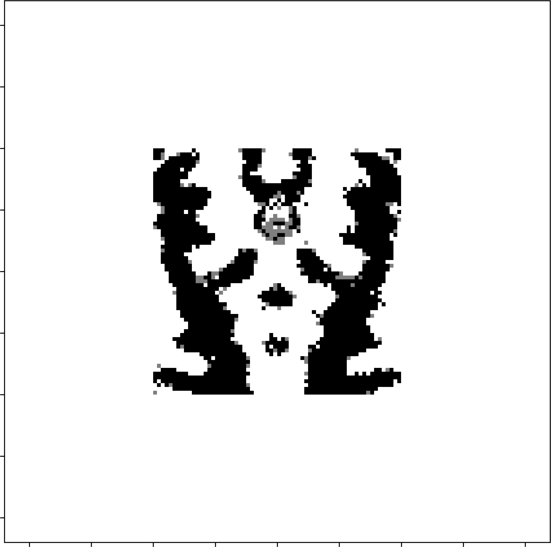
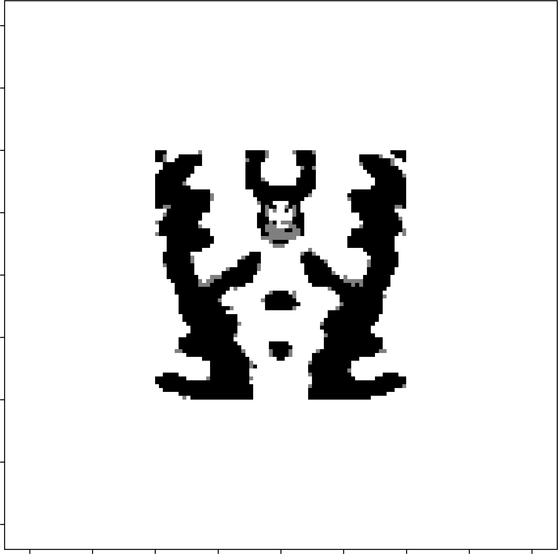
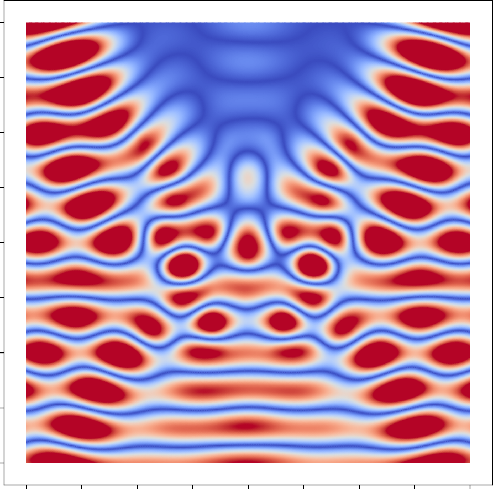
(a)

(b)

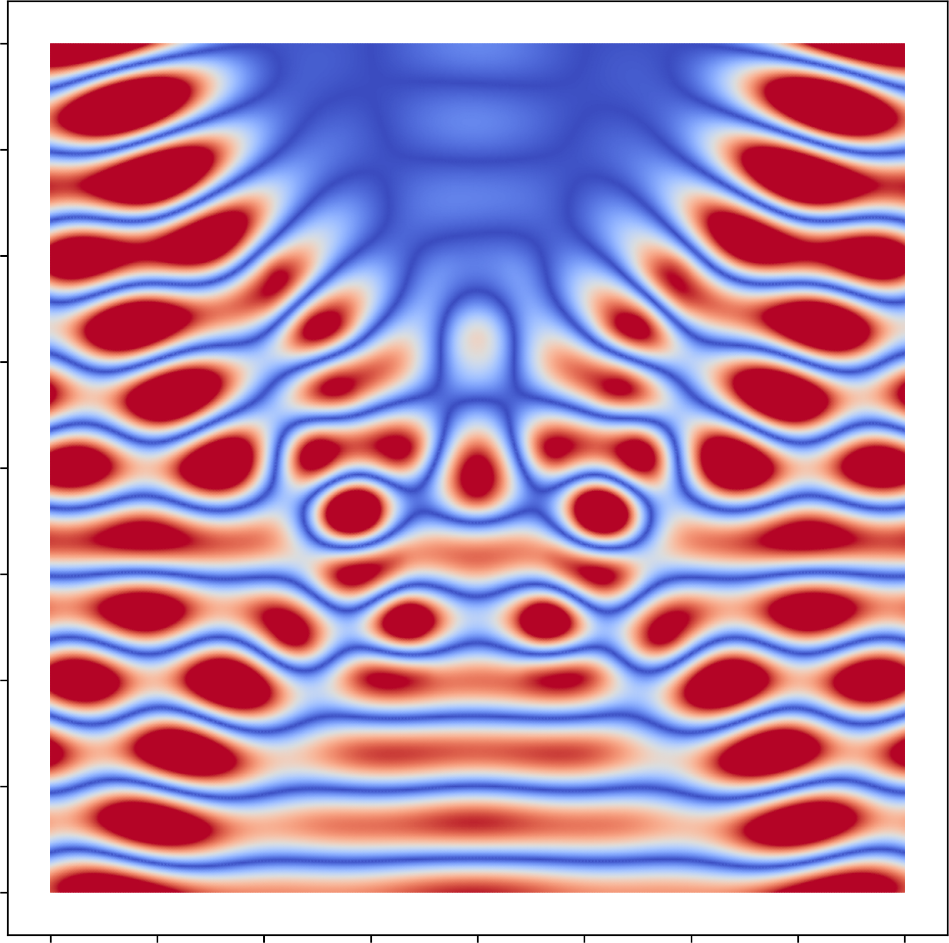
(c)

Figure 2: Computed controls and corresponding moduli of the real parts of the solution of the PDE constraining (5.1) for $\delta=0$ and $k=7$. (2(a)): Baseline solution on uniform grid, (2(b)): Solution with primal heuristic on non-uniform grid, (2(c)): Solution with primal heuristic and separators on non-uniform grid. Note that no baseline solution could be computed on the non-uniform grid within the prescribed time limit of one hour.

6 Acknowledgment

C. Kirches, F. Bestehorn and P. Manns acknowledge funding by Deutsche Forschungsgemeinschaft (DFG) through Priority Programme 1962 (grant Ki 1839/1-2).

7 Conclusion

We proposed a non-uniform grid refinement strategy that preserves the approximation properties of the combinatorial integral approximation. Using these grids inside switching cost aware rounding on instances of a test problem that is defined on a multi-dimensional domain, we obtained mixed-integer programs with fewer variables and better tractability, i.e. better runtime performance, when treating them with a general purpose integer programming solver. We were generally able to improve the solution process of the integer program by adding valid linear inequalities and applying the efficient combinatorial algorithm that is available for the one-dimensional case as a heuristic to the multi-dimensional problem. However, the considered instances can still not be solved to global optimality within acceptable time limits and large duality gaps remain. Moreover, the visible difference between the computed solutions are very small.

References

- [1] S. Balay, S. Abhyankar, M. F. Adams, J. Brown, P. Brune, K. Buschelman, L. Dalcin, V. Eijkhout, W. D. Gropp, D. Karpeyev, D. Kaushik, M. G. Knepley, D. A. May, L. Curfman McInnes, R. T. Mills, T. Munson, K. Rupp, P. Sanan, B. F. Smith, S. Zampini, H. Zhang, and H. Zhang. PETSc Users Manual. Technical Report ANL-95/11 - Revision 3.11, Argonne National Laboratory, 2019.
- [2] Felix Bestehorn. Combinatorial algorithms and complexity of rounding problems arising in mixed-integer optimal control. PhD thesis, Technical University of Braunschweig, 2021.
- [3] Felix Bestehorn, Christoph Hansknecht, Christian Kirches, and Paul Manns. A switching cost aware rounding method for relaxations of mixed-integer optimal control problems. In 2019 IEEE 58th Conference on Decision and Control (CDC), pages 7134–7139. IEEE, 2019.
- [4] Felix Bestehorn, Christoph Hansknecht, Christian Kirches, and Paul Manns. Mixed-integer optimal control problems with switching costs: a shortest path approach. Mathematical Programming, 188(2):621–652, 2021.
- [5] Felix Bestehorn, Christoph Hansknecht, Christian Kirches, and Paul Manns. Switching cost aware rounding for relaxations of mixed-integer optimal control problems: The 2-d case. IEEE Control Systems Letters, 6:548–553, 2021.
- [6] Felix Bestehorn and Christian Kirches. Matching algorithms and complexity results for constrained mixed-integer optimal control with switching costs. Optimization Online Preprint 2020/10/8059, 2020.
- [7] Ksenia Bestuzheva, Mathieu Besançon, Wei-Kun Chen, Antonia Chmiela, Tim Donkiewicz, Jasper van Doornmalen, Leon Eifler, Oliver Gaul, Gerald Gamrath, Ambros Gleixner, et al. The scip optimization suite 8.0. arXiv preprint arXiv:2112.08872, 2021.
- [8] P. E. Farrell, D. A. Ham, S. W. Funke, and M. E. Rognes. Automated derivation of the adjoint of high-level transient finite element programs. SIAM Journal on Scientific Computing, 35(4):C369–C393, 2013.
- [9] Alexey Fedorovich Filippov. On certain questions in the theory of optimal control. Journal of the Society for Industrial and Applied Mathematics, Series A: Control, 1(1):76–84, 1962.
- [10] Matthias Gerdts. Solving mixed-integer optimal control problems by branch&bound: a case study from automobile test-driving with gear shift. Optimal Control Applications and Methods, 26(1):1–18, 2005.
- [11] Simone Göttlich, Andreas Potschka, and Ute Ziegler. Partial outer convexification for traffic light optimization in road networks. SIAM Journal on Scientific Computing, 39(1):B53–B75, 2017.
- [12] Gurobi Optimization, LLC. Gurobi Optimizer Reference Manual, 2020.
- [13] Falk M Hante. Mixed-Integer Optimal Control for PDEs: Relaxation via Differential Inclusions and Applications to Gas Network Optimization. In Mathematical Modelling, Optimization, Analytic and Numerical Solutions, pages 157–171. Springer, 2020.
- [14] Falk M Hante and Sebastian Sager. Relaxation methods for mixed-integer optimal control of partial differential equations. Computational Optimization and Applications, 55(1):197–225, 2013.
- [15] Mark Hartmann and Todd Olmstead. Solving sequential knapsack problems. Operations research letters, 13(4):225–232, 1993.
- [16] J. Haslinger and R.A.E. Mäkinen. On a topology optimization problem governed by two-dimensional Helmholtz equation. Computational Optimization and Applications, 62(2):517–544, 2015.
- [17] Christopher Hojny, Tristan Gally, Oliver Habeck, Hendrik Lüthen, Frederic Matter, Marc E Pfetsch, and Andreas Schmitt. Knapsack polytopes: a survey. Annals of Operations Research, 292(1):469–517, 2020.
- [18] Michael Jung. Relaxations and approximations for mixed-integer optimal control. PhD thesis, Heidelberg University, 2014.
- [19] Christian Kirches, Felix Lenders, and Paul Manns. Approximation properties and tight bounds for constrained mixed-integer optimal control. SIAM Journal on Control and Optimization, 58(3):1371–1402, 2020.
- [20] Christian Kirches, Paul Manns, and Stefan Ulbrich. Compactness and convergence rates in the combinatorial integral approximation decomposition. Mathematical Programming, 188(2):569–598, 2021.
- [21] Christian Kirches, Sebastian Sager, Hans Georg Bock, and Johannes P Schlöder. Time-optimal control of automobile test drives with gear shifts. Optimal Control Applications and Methods, 31(2):137–153, 2010.
- [22] S. Leyffer, P. Manns, and M. Winckler. Convergence of sum-up rounding schemes for cloaking problems governed by the Helmholtz equation. Computational Optimization and Applications, pages 1–29, 2021.
- [23] Joram Lindenstrauss. A short proof of Liapounoff’s convexity theorem. Journal of Mathematics and Mechanics, 15(6):971–972, 1966.
- [24] Alexey Andreevich Lyapunov. On completely additive vector functions. Izv. Akad. Nauk SSSR, 4:465–478, 1940.
- [25] Paul Manns and Christian Kirches. Improved regularity assumptions for partial outer convexification of mixed-integer PDE-constrained optimization problems. ESAIM: Control, Optimisation and Calculus of Variations, 26:32, 2020.
- [26] Paul Manns and Christian Kirches. Multidimensional sum-up rounding for elliptic control systems. SIAM Journal on Numerical Analysis, 58(6):3427–3447, 2020.
- [27] Paul Manns, Christian Kirches, and Felix Lenders. Approximation properties of sum-up rounding in the presence of vanishing constraints. Mathematics of Computation, 90(329):1263–1296, 2021.
- [28] Alexander Martin, Markus Möller, and Susanne Moritz. Mixed integer models for the stationary case of gas network optimization. Mathematical Programming, 105(2):563–582, 2006.
- [29] David Pisinger and Paolo Toth. Knapsack problems. In Handbook of combinatorial optimization, pages 299–428. Springer, 1998.
- [30] Yves Pochet and Robert Weismantel. The sequential knapsack polytope. SIAM Journal on Optimization, 8(1):248–264, 1998.
- [31] F. Rathgeber, D. A. Ham, D. Mitchell, M. Lange, F. Luporini, A. T. T. McRae, G.-T. Bercea, G. R. Markall, and Paul H. J. Kelly. Firedrake: automating the finite element method by composing abstractions. ACM Trans. Math. Softw., 43(3):24:1–24:27, 2016.
- [32] Sebastian Sager. Numerical methods for mixed-integer optimal control problems. Citeseer, 2005.
- [33] Sebastian Sager, Hans Georg Bock, and Moritz Diehl. The integer approximation error in mixed-integer optimal control. Mathematical programming, 133(1):1–23, 2012.
- [34] Sebastian Sager, Hans Georg Bock, Moritz Diehl, Gerhard Reinelt, and Johannes P Schlöder. Numerical methods for optimal control with binary control functions applied to a lotka-volterra type fishing problem. In Recent Advances in Optimization, pages 269–289. Springer, 2006.
- [35] Sebastian Sager and Clemens Zeile. On mixed-integer optimal control with constrained total variation of the integer control. Computational Optimization and Applications, 78(2):575–623, 2021.
- [36] Tadeusz Ważewski. On an optimal control problem. Differential Equations and their Applications, pages 229–242, 1963.
- [37] Victor M Zavala, Jianhui Wang, Sven Leyffer, Emil M Constantinescu, Mihai Anitescu, and Guenter Conzelmann. Proactive energy management for next-generation building systems. Proceedings of SimBuild, 4(1):377–385, 2010.